convolutional neural network in practice
TRANSCRIPT

Preliminaries

Buzz words nowadays
AIDeep
learning
Big dataMachine learning
Reinforcement Learning
???

Glossary of AI terms
From Roger Parloff, WHY DEEP LEARNING IS SUDDENLY CHANGING YOUR LIFE (Fortune, 2016).

Definitions
What is AI ?
“Artificial intelligence is that activity devoted to making machines intelligent, and intelligence is that quality that enables an entity to function appropriately and with foresight in its environment.”
Nils J. Nilsson, The Quest for Artificial Intelligence: A History of Ideas and Achievements (Cambridge, UK: Cambridge University Press, 2010).
“a computerized system that exhibits behavior that is commonly thought of as requiring intelligence”
Executive Office of the President National Science and Technology Council Committee on Technology: PREPARING FOR THE FUTURE OF ARTIFICIAL INTELLIGENCE (2016).
“any technique that enables computers to mimic human intelligence”
Roger Parloff, WHY DEEP LEARNING IS SUDDENLY CHANGING YOUR LIFE (Fortune, 2016).

My diagram of AI terms
Environment
Data, Rules, Feedbacks ...
Teaching
Self-Learning,Engineering
...
AI
y = f(x)
Catf F18f
Past, Present of AI

Decades-old technology
● Long long history. From 1940s …
● But,
○ Before Oct. 2012.
○ After Oct. 2012.

Venn diagram of AI terms
From Ian Goodfellow, Deep Learning (MIT press, 2016).
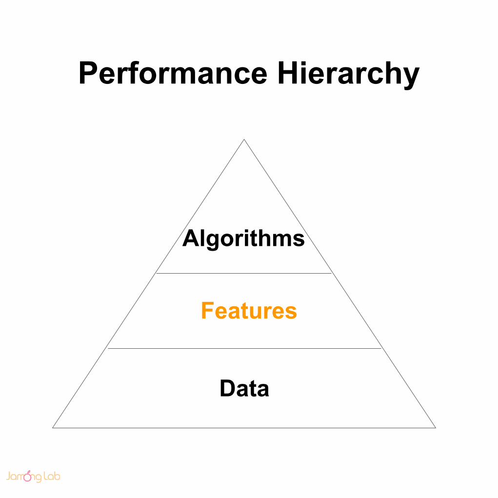
Performance Hierarchy
Data
Features
Algorithms

Flowcharts of AI
From Ian Goodfellow, Deep Learning (MIT press, 2016).
E2E(end-to-end)

Image recognition error rate
From https://www.nervanasys.com/deep-learning-and-the-need-for-unified-tools/
2012

Speech recognition error rate
2012

5 Tribes of AI researchers
Symbolists(Rule, Logic-based)
Connectionists(PDP assumption)
Bayesians EvolutionistsAnalogizers
vs.

Deep learning has had a long and rich history !
● 3 re-brandings.
○ Cybernetics ( 1940s ~ 1960s )
○ Artificial Neural Networks ( 1980s ~ 1990s)
○ Deep learning ( 2006 ~ )

Nothing new !
● Alexnet 2012
○ based on CNN ( LeCunn, 1989 )
● Alpha Go
○ based on Reinforcement learning and
MCTS ( Sutton, 1998 )

So, why now ?
● Computing Power
● Large labelled dataset
● Algorithm

Size of neural networks
From Ian Goodfellow, Deep Learning (MIT press, 2016).
Singularity or Transcendence ?

Depth is KING !

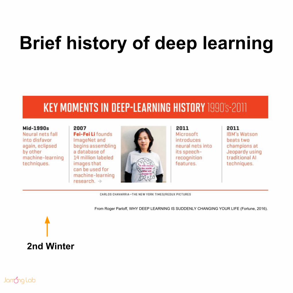
Brief history of deep learning
From Roger Parloff, WHY DEEP LEARNING IS SUDDENLY CHANGING YOUR LIFE (Fortune, 2016).
1st Boom 2nd Boom1st Winter

Brief history of deep learning
From Roger Parloff, WHY DEEP LEARNING IS SUDDENLY CHANGING YOUR LIFE (Fortune, 2016).
Brief history of deep learning
From Roger Parloff, WHY DEEP LEARNING IS SUDDENLY CHANGING YOUR LIFE (Fortune, 2016).
2nd Winter

Brief history of deep learning
From Roger Parloff, WHY DEEP LEARNING IS SUDDENLY CHANGING YOUR LIFE (Fortune, 2016).
3rd Boom

Brief history of deep learning
From Roger Parloff, WHY DEEP LEARNING IS SUDDENLY CHANGING YOUR LIFE (Fortune, 2016).
So, when 3rd winter ?
Nope !!!
● Features are mandatory in every AI problem.
● Deep learning is cheap learning! (Though someone can disprove the PDP assumptions, deep learning is the best practical tool in representation learning.)

Biz trends after Oct.2012.
● 4 big players leading this sector.
● Bloody hiring war.○ Along the lines of NFL football players.

Biz trend after Oct.2012.
● 2 leading research firms.
● 60+ startups

Biz trend after Oct.2012.

Future of AI

Venn diagram of ML
From David silver, Reinforcement learning (UCL cource on RL, 2015).

Unsupervised & Reinforcement Learning
● 2 leading research firms focus on:
○ Generative Models
○ Reinforcement Learning

Towards General Artificial Intelligence

Towards General Artificial Intelligence
Strong AI vs. Weak AIGeneral AI vs. Narrow AI
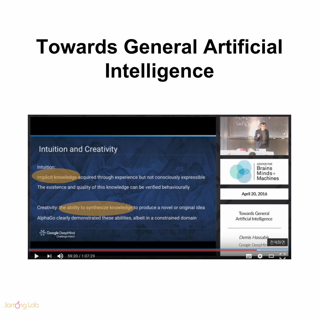
Towards General Artificial Intelligence

Towards General Artificial Intelligence

Generative Adversarial Network
Xi Chen et al, InfoGAN: Interpretable Representation Learning by Information Maximizing Generative Adversarial Nets ( 2016 )

Generative Adversarial Network
(From https://github.com/buriburisuri/supervised_infogan 2016)

So what can we do with AI?
● Simply, it’s sophisticated software
writing software.
True personalization at scale!!!
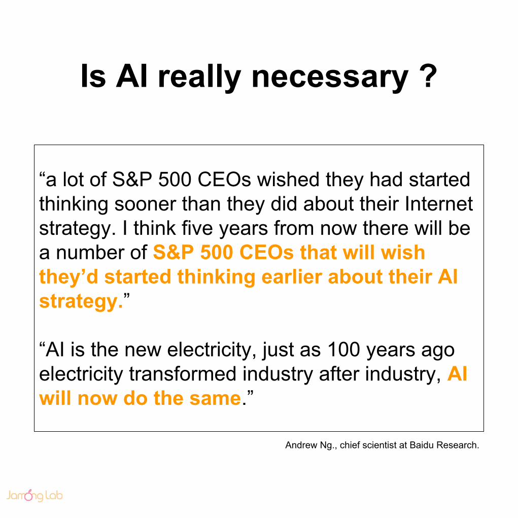
Is AI really necessary ?
“a lot of S&P 500 CEOs wished they had started thinking sooner than they did about their Internet strategy. I think five years from now there will be a number of S&P 500 CEOs that will wish they’d started thinking earlier about their AI strategy.”
“AI is the new electricity, just as 100 years ago electricity transformed industry after industry, AI will now do the same.”
Andrew Ng., chief scientist at Baidu Research.

Conclusion
Computers have opened their eyes.

Convolution Neural Network

Convolution Neural Network
● Motivation
○ Sparse connectivity
■ smaller kernel size
○ Parameter sharing
■ shared kernel
○ Equivariant representation
■ convolution operation

Fully Connected(Dense) Neural Network
● Typical 3-layer fully connected neural network
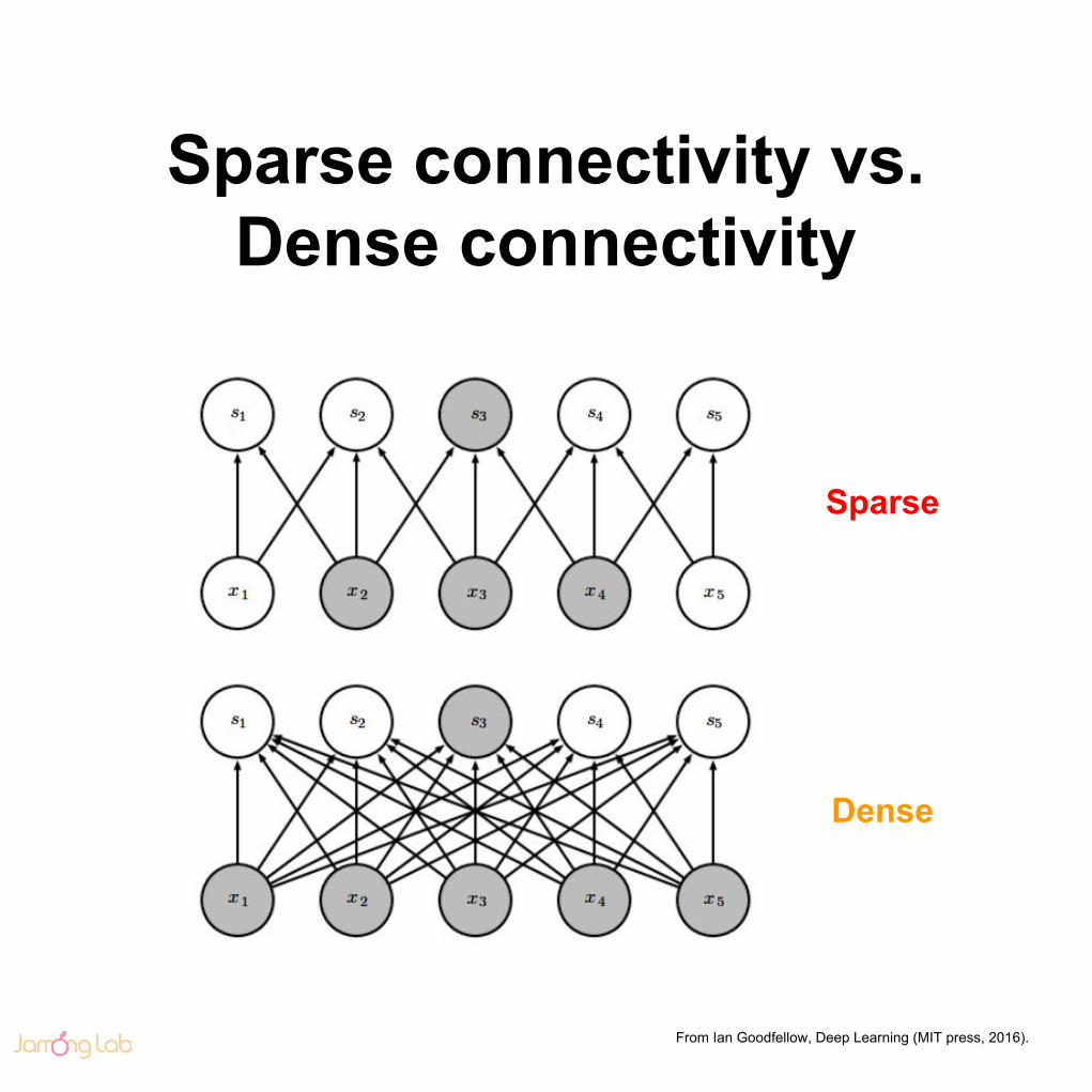
Sparse connectivity vs.Dense connectivity
Sparse
Dense
From Ian Goodfellow, Deep Learning (MIT press, 2016).

Parameter sharing
(x1, s1) ~ (x5, s5) share a single
parameter
From Ian Goodfellow, Deep Learning (MIT press, 2016).

Equivariant representation
Convolution operation
satisfies equivariant property.

A bit of history
From : http://cs231n.stanford.edu/slides/winter1516_lecture6.pdf

A bit of history
From : http://cs231n.stanford.edu/slides/winter1516_lecture6.pdf

A bit of history
From : http://cs231n.stanford.edu/slides/winter1516_lecture6.pdf
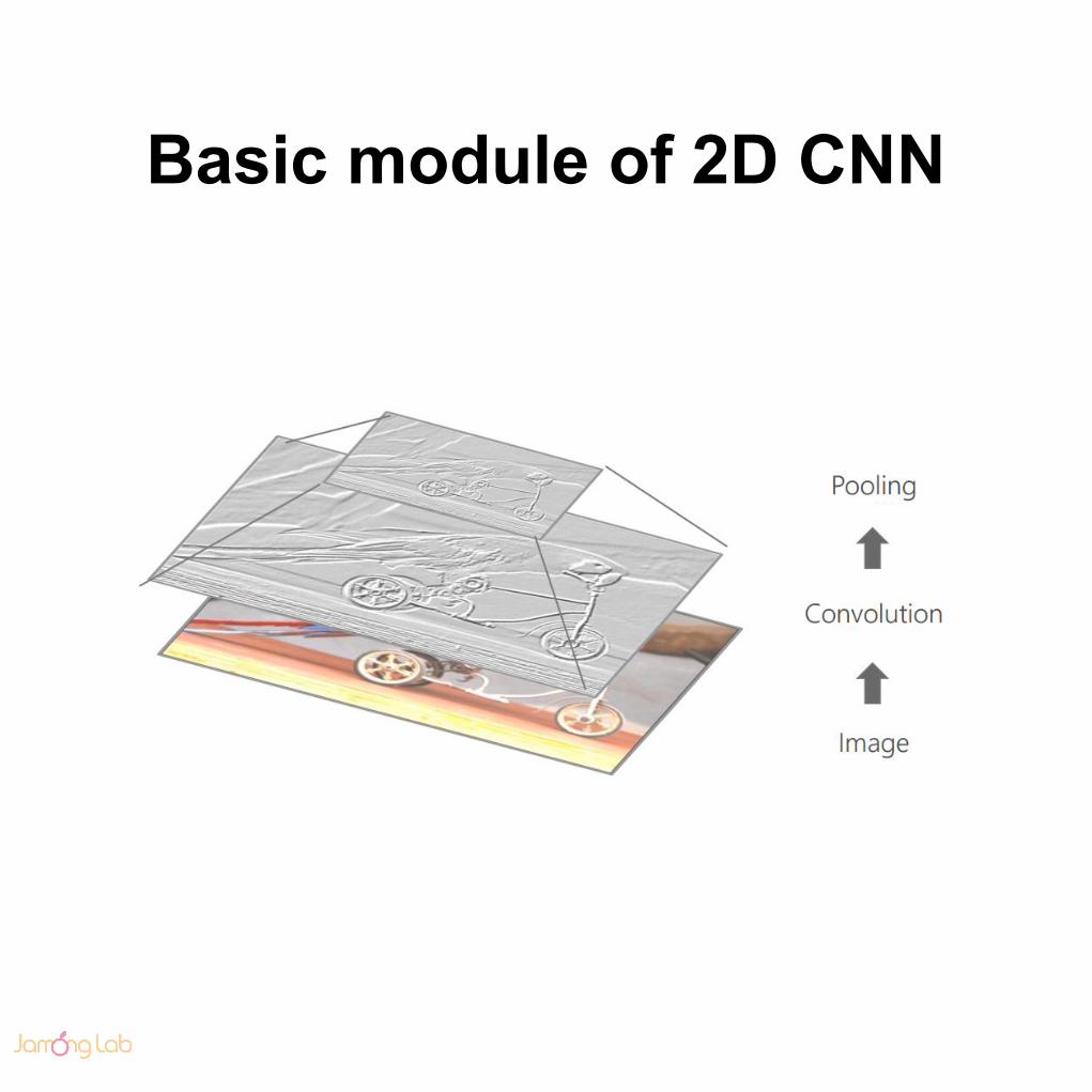
Basic module of 2D CNN

Pooling
● Average pooling = L1 pooling
● Max pooling = infinity norm pooling

Max Pooling
● To improve translation invariance.

Parameters of convolution
● Kernel size○ ( row, col, in_channel, out_channel)
● Padding
○ SAME, VALID, FULL
● Stride
○ if S > 1, use even kernel size F >
S * 2

1 dimensional convolution
pad(P=1) pad(P=1) pad(P=1)
stride(S=1)
kernel(F=3)
stride(S=2)
● ‘SAME’(or ‘HALF’) pad size = (F - 1) * S / 2● ‘VALID’ pad size = 0● ‘FULL’ pad size : not used nowadays

2 dimensional convolution
From : https://github.com/vdumoulin/conv_arithmetic
pad = ‘VALID’, F = 3, S = 1

2 dimensional convolution
From : https://github.com/vdumoulin/conv_arithmetic
pad = ‘SAME’, F = 3, S = 1

2 dimensional convolution
From : https://github.com/vdumoulin/conv_arithmetic
pad = ‘SAME’, F = 3, S = 2

Artifacts of strides
From : http://distill.pub/2016/deconv-checkerboard/
F = 3, S = 2

Artifacts of strides
F = 4, S = 2
From : http://distill.pub/2016/deconv-checkerboard/

Artifacts of strides
From : http://distill.pub/2016/deconv-checkerboard/
F = 4, S = 2
Pooling vs. Striding
● Same in the downsample aspect
● But, different in the location aspect
○ Location is lost in Pooling
○ Location is preserved in Striding
● Nowadays, striding is more popular
○ some kind of learnable pooling

Kernel initialization
● Random number between -1 and 1
○ Orthogonality ( I.I.D. )
○ Uniform or Gaussian random
● Scale is paramount.
○ Adjust such that out(activation)
values have mean 0 and variance 1
○ If you encounter NaN, that may be
because of ill scale.

Gabor Filter

Activation results
Initialization guide
● Xavier(or Glorot) initialization
○ http://jmlr.org/proceedings/papers/v9/glorot10a/glorot10a
● He initialization
○ Good for RELU nonlinearity
○ https://arxiv.org/abs/1502.01852
● Use batch normalization if possible○ Immune to ill-scaled initialization

Image classification

Guide
● Start from robust baseline
○ 3 choices
■ VGG, Inception-v3, Resnet
● Smaller and deeper
● Towards getting rid of POOL and
final dense layer
● BN and skip connection are popular

VGG
VGG
● https://arxiv.org/abs/1409.1556
● VGG-16 is good start point.
○ apply BN if you train from scratch
● Image input : 224x224x3 ( -1 ~ 1 )
● Final outputs
○ conv5 : 7x7x512
○ fc2 : 4096
○ sm : 1000
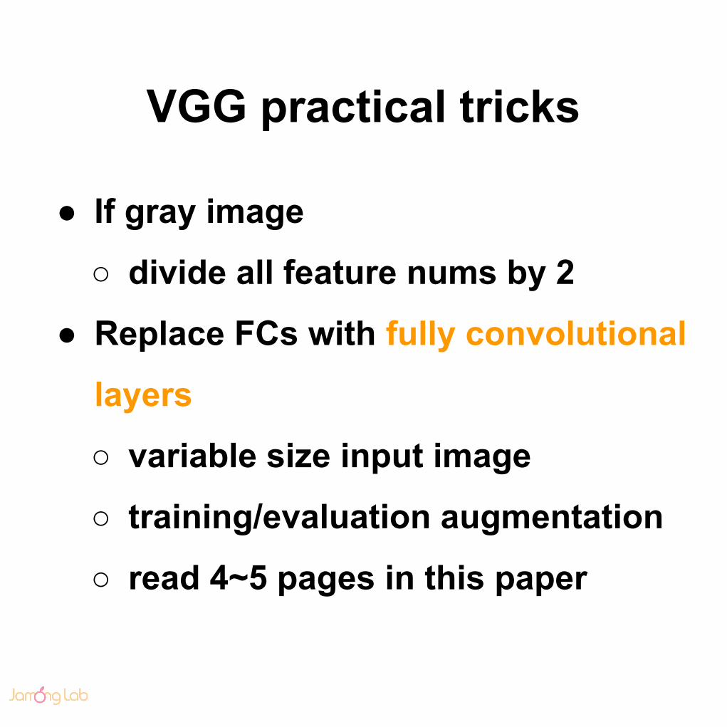
VGG practical tricks
● If gray image
○ divide all feature nums by 2
● Replace FCs with fully convolutional
layers
○ variable size input image
○ training/evaluation augmentation
○ read 4~5 pages in this paper

Fully connected layer
● conv5 output : 7x7x512
● Fully connected layer
○ flatten : 1x25088
○ fc1 weight: 25088x4096
■ output : 1x4096
○ fc2 weight: 4096x4096
■ output : 1x4096
○ Fixed size image only

Fully convolutional layer● conv5 output : 7x7x512
● Fully convolutional layer
○ fc1 ← conv 7x7@4096
■ output : (row-6)x(col-6)x4096
○ fc2 ← conv 1x1@4096
■ output : (row-6)x(col-6)x4096
○ Global average pooling
■ output : 1x1x4096
○ Variable sized images

VGG Fully convolutional layer
From : https://github.com/buriburisuri/sugartensor/blob/master/sugartensor/sg_net.py

Google Inception

Google Inception● https://arxiv.org/pdf/1512.00567.pdf
● Bottlenecked architecture.
○ 1x1 conv
○ latest version : v5 ( v3 is popular )
● Image input : 224x224x3 ( -1 ~ 1 )
● Final output
○ conv5 : 7x7x1024 ( or 832 )
○ fc2 : 1024
○ sm : 1000

Batch Normalization● https://arxiv.org/pdf/1502.03167.pdf
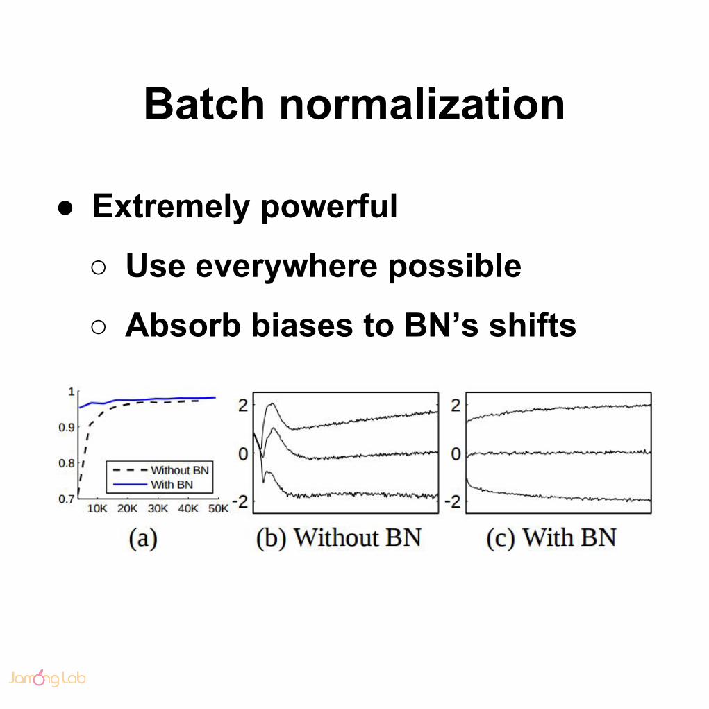
Batch normalization
● Extremely powerful
○ Use everywhere possible
○ Absorb biases to BN’s shifts
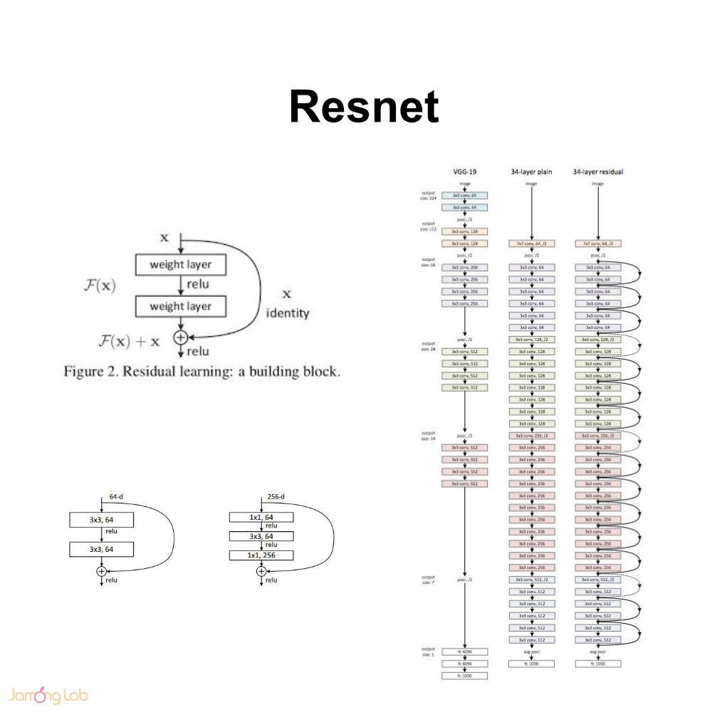
Resnet

Resnet
● https://arxiv.org/pdf/1512.03385v1.pdf
● Residual block
○ skip connection + stride
○ bottleneck block
● Image input : 224x224x3 ( -1 ~ 1 )
● Final output
○ conv5 : 7x7x2048
○ fc2 : 1x1x2048 ( average pooling )
○ sm : 1000

Resnet
● Very deep using skip connection○ Now, v2 - 1001 layer architecture
● Now, Resnet-152 v2 is the de-facto standard
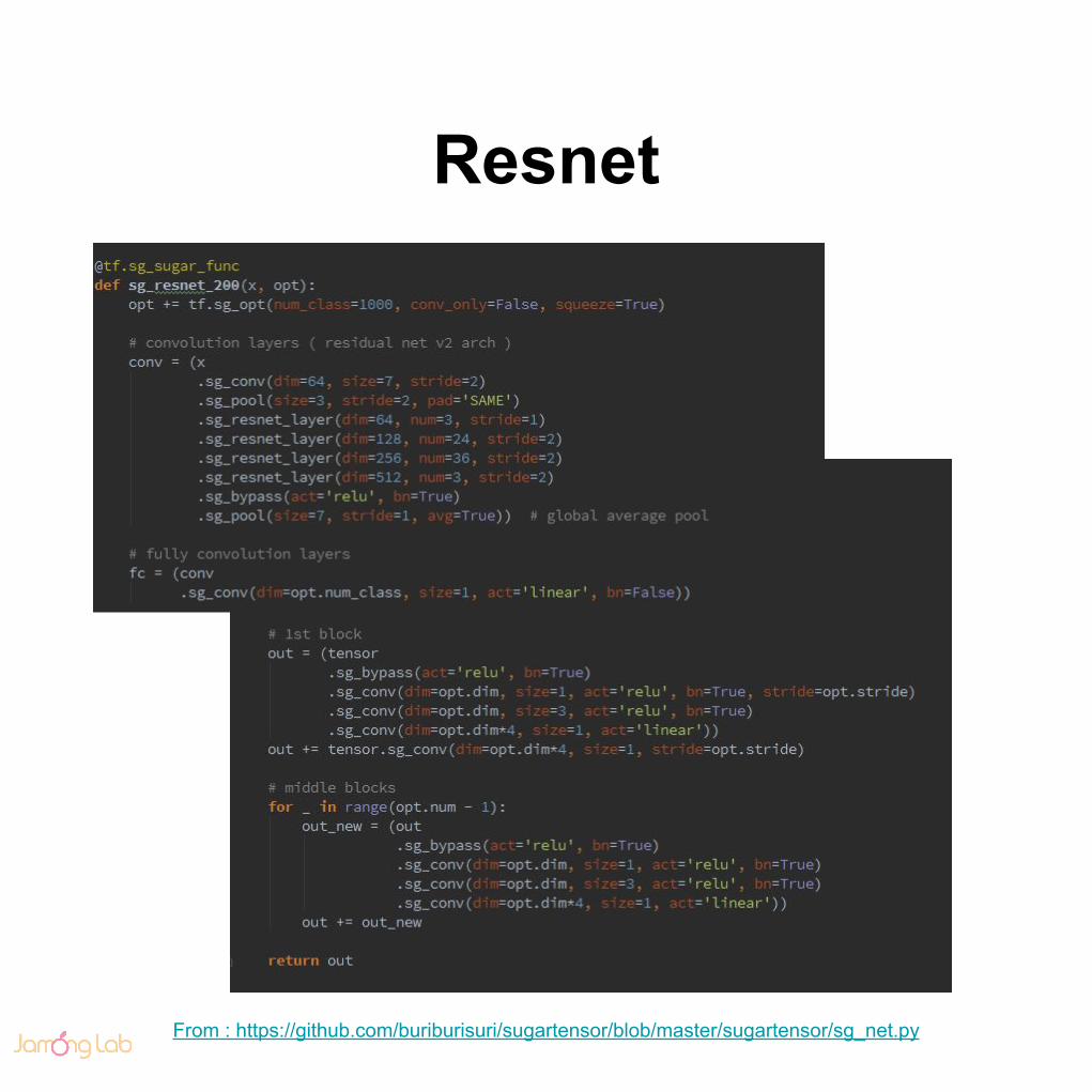
Resnet
From : https://github.com/buriburisuri/sugartensor/blob/master/sugartensor/sg_net.py

Summary
● Start from Resnet-50
● Use He’s initialization
● learning rate : 0.001 (with BN), 0.0001
(without BN)
● Use Adam ( should be alpha < beta ) optim
○ alpha=0.9, beta=0.999 (with easy training)
○ alpha=0.5, beta=0.95 (with hard training)

Summary
● Minimize hyper-parameter tuning or
architecture modification.
○ Deep learning is highly nonlinear and
count-intuitive
○ Grid or random search is expensive

Visualization

Kernel visualization
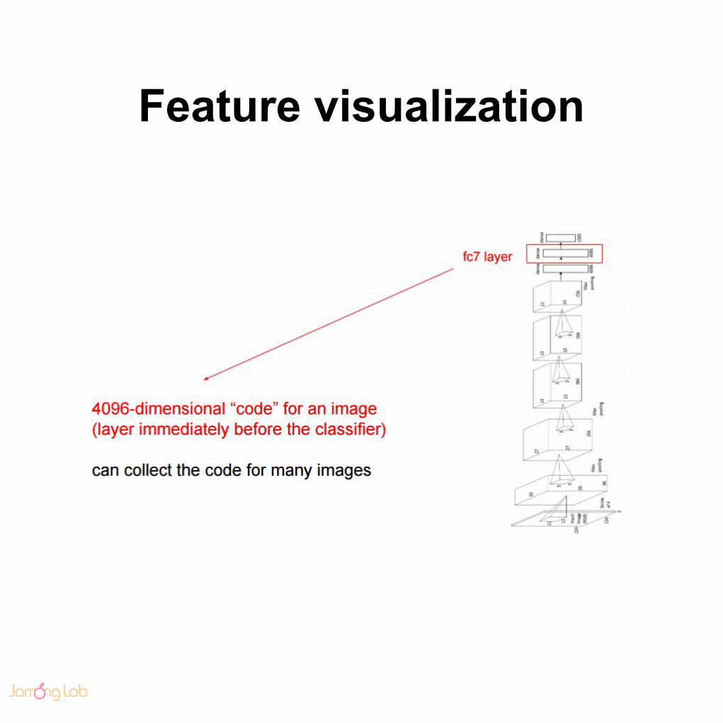
Feature visualization

t-SNE visualization
https://lvdmaaten.github.io/tsne/

Occlusion chart
https://arxiv.org/abs/1311.2901

Activation chart
http://yosinski.com/deepvishttps://www.youtube.com/watch?v=AgkfIQ4IGaM

CAM : Class Activation Map
http://cnnlocalization.csail.mit.edu/
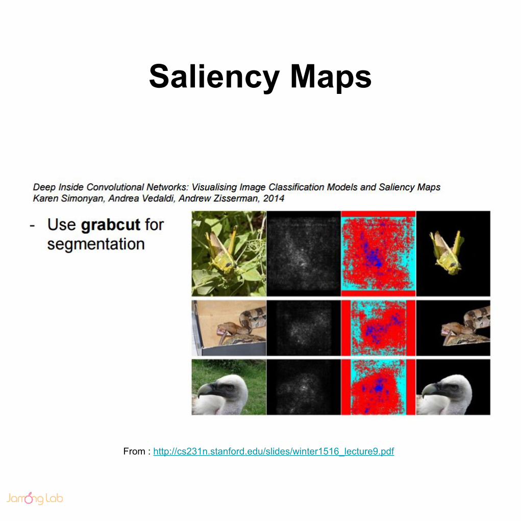
Saliency Maps
From : http://cs231n.stanford.edu/slides/winter1516_lecture9.pdf

Deconvolution approach
From : http://cs231n.stanford.edu/slides/winter1516_lecture9.pdf

Augmentation

Augmentation
● 3 types of augmentation
○ Traing data augmentation
○ Evaluation augmentation
○ Label augmentation
● Augmentation is mandatory○ If you have really big data, then augment
data and increase model capacity

Training Augmentation● Random crop/scale
○ random L in range [256, 480]
○ Resize training image, short side = L
○ Sample random 224x224 patch

Training Augmentation● Random flip/rotate
● Color jitter

Training Augmentation● Random flip/rotate
● Color jitter
● Random occlude

Testing Augmentation● 10-crop testing ( VGG )
○ average(or max) scores

Testing Augmentation
● Multi-scale testing
○ Fully convolutional layer is mandatory
○ Random L in range [224, 640]
○ Resize training image such that short side
= L
○ Average(or max) scores
● Used in Resnet
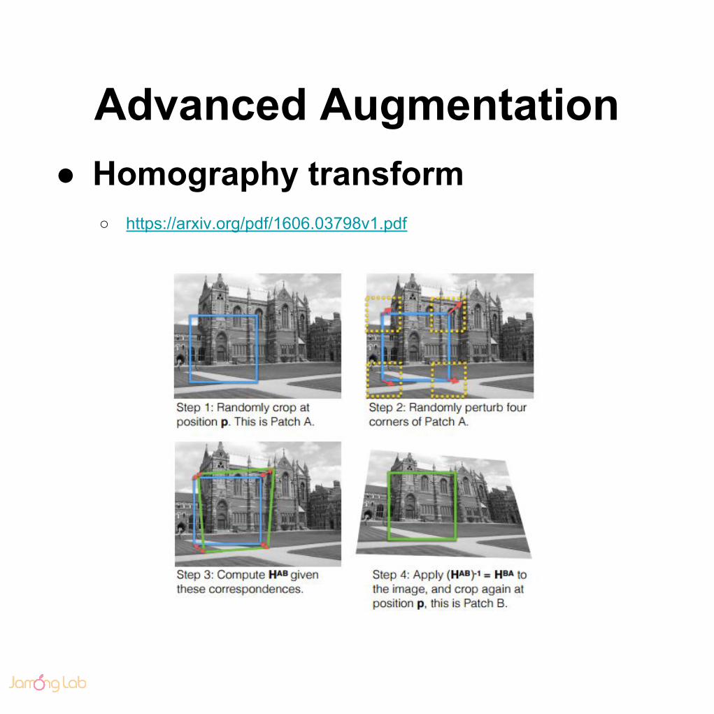
Advanced Augmentation● Homography transform
○ https://arxiv.org/pdf/1606.03798v1.pdf
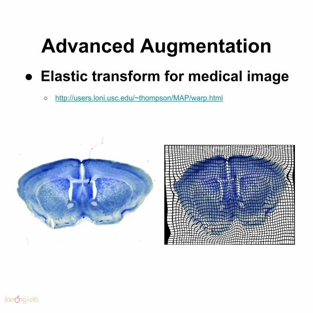
Advanced Augmentation● Elastic transform for medical image
○ http://users.loni.usc.edu/~thompson/MAP/warp.html

Augmentation in action

Other Augmentation● Be aggressive and creative!

Feature level Augmentation● Exploit equivariant property of CNN
○ Xu shen, “Transform-Invariant Convolutional Neural Networks for Image Classification and
Search”, 2016
○ Hyo-Eun Kim, “Semantic Noise Modeling for Better Representation Learning”, 2016

Image Localization

Localization and Detection
From : http://cs231n.stanford.edu/slides/winter1516_lecture8.pdf

Classification + Localization
From : http://cs231n.stanford.edu/slides/winter1516_lecture8.pdf

Simple recipe
CE loss
L2(MSE) loss
Joint-learning ( Multi-task learning )or
Separate learning
From : http://cs231n.stanford.edu/slides/winter1516_lecture8.pdf

Regression head position
From : http://cs231n.stanford.edu/slides/winter1516_lecture8.pdf

Multiple objects detection
From : http://cs231n.stanford.edu/slides/winter1516_lecture8.pdf

R-CNN
From : http://cs231n.stanford.edu/slides/winter1516_lecture8.pdf

Fast R-CNN
From : http://cs231n.stanford.edu/slides/winter1516_lecture8.pdf

Faster R-CNN
From : http://cs231n.stanford.edu/slides/winter1516_lecture8.pdf

Faster R-CNN
● https://arxiv.org/pdf/1506.01497.pdf
● de-facto standard
From : http://cs231n.stanford.edu/slides/winter1516_lecture8.pdf

Segmentation

Semantic Segmentation
From : http://cs231n.stanford.edu/slides/winter1516_lecture13.pdf

Naive recipe
From : http://cs231n.stanford.edu/slides/winter1516_lecture13.pdf

Fast recipe
From : http://cs231n.stanford.edu/slides/winter1516_lecture13.pdf

Multi-scale refinement
From : http://cs231n.stanford.edu/slides/winter1516_lecture13.pdf

Recurrent refinement
From : http://cs231n.stanford.edu/slides/winter1516_lecture13.pdf

Upsampling
From : http://cs231n.stanford.edu/slides/winter1516_lecture13.pdf
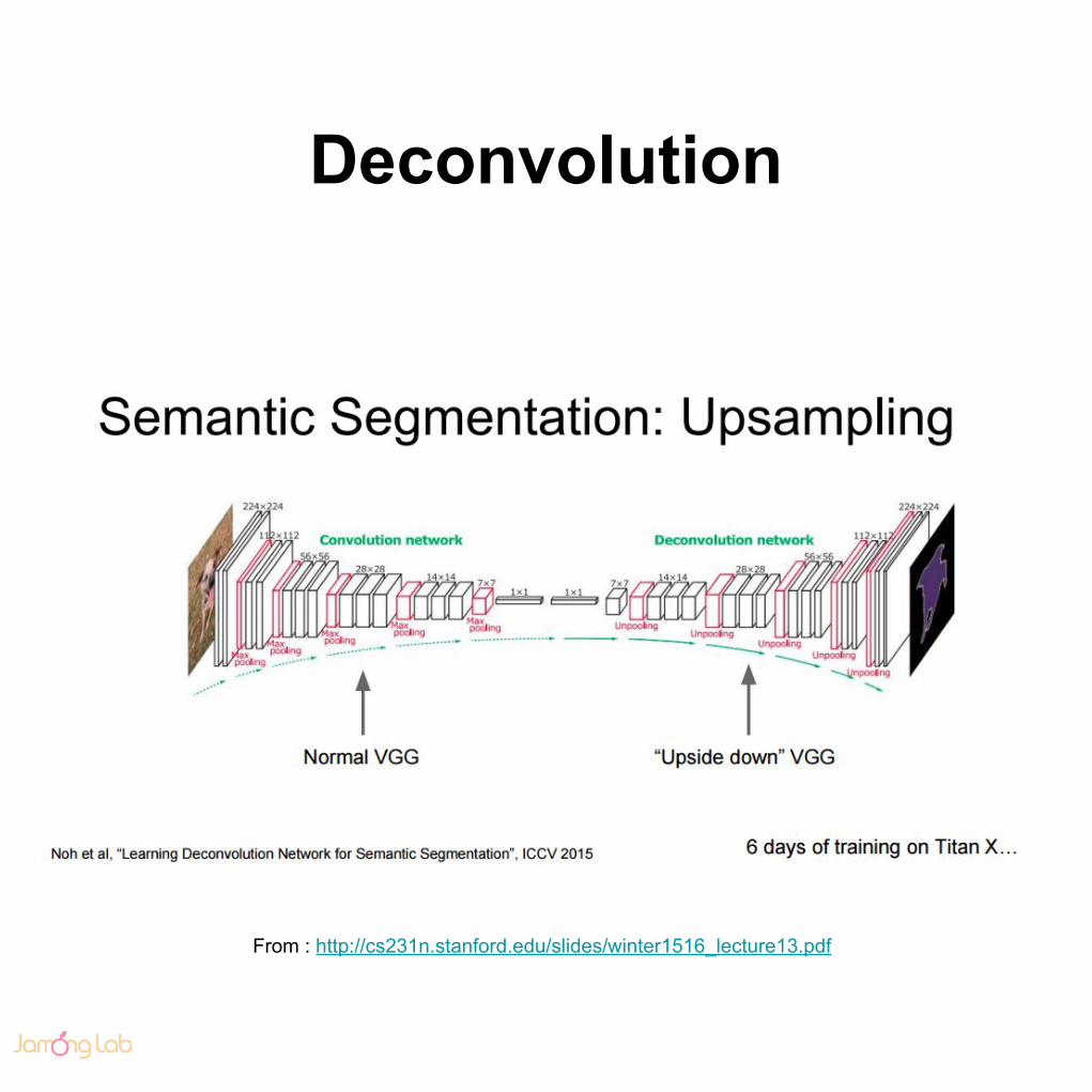
Deconvolution
From : http://cs231n.stanford.edu/slides/winter1516_lecture13.pdf

Skip connection
Olaf, U-Net: Convolutional Networks for Biomedical Image Segmentation, 2015

Instance Segmentation
From : http://cs231n.stanford.edu/slides/winter1516_lecture13.pdf

R-CNN
From : http://cs231n.stanford.edu/slides/winter1516_lecture13.pdf

Hypercolumns
From : http://cs231n.stanford.edu/slides/winter1516_lecture13.pdf

Cascades
From : http://cs231n.stanford.edu/slides/winter1516_lecture13.pdf

Deconvolution
● Learnable upsampling
○ resize * 2 + normal convolution
○ controversial names■ deconvolution, convolution transpose, upconvolution,
backward strided convolution, ½ strided convolution
○ Artifacts by strides and kernel sizes■ http://distill.pub/2016/deconv-checkerboard/
○ Restrict the freedom of architectures


½ strided(sub-pixel) convolution
From : https://arxiv.org/abs/1609.07009

ESPCN ( Efficient Sub-pixel CNN)
Periodic shuffle
Wenzhe, Real-Time Single Image and Video Super-Resolution Using and Efficient Sub-Pixel Convolutional Neural Network, 2016

L2 loss issue
Christian, Photo-Realistic Single Image Super-Resolution Using a Generative Adversarial Network, 2016

SRGAN
https://github.com/buriburisuri/SRGAN

Videos

ST-CNN
From : http://cs231n.stanford.edu/slides/winter1516_lecture14.pdf

ST-CNN
From : http://cs231n.stanford.edu/slides/winter1516_lecture14.pdf

Long-Time ST-CNN
From : http://cs231n.stanford.edu/slides/winter1516_lecture14.pdf

Long-Time ST-CNN
From : http://cs231n.stanford.edu/slides/winter1516_lecture14.pdf

Summary
● Model temporal motion locally ( 3D CONV )
● Model temporal motion globally ( RNN )
● Hybrids of both
● IMHO, RNN will be replaced with 1D
convolution dilated (atrous convolution)
Unsupervised learning

Stacked Autoencoder

Stacked Autoencoder
● Blurry artifacts caused by L2 loss

Variational Autoencoder
● Generative model
● Blurry artifacts caused by L2 loss

Variational Autoencoder
● SAE with mean and variance regularizer
● Bayesian meets deep learning

Generative Model
● Find realistic generating function G(x) by deep learning !!!
y = G(x)
G : Generating functionx : Factors
y : Output data
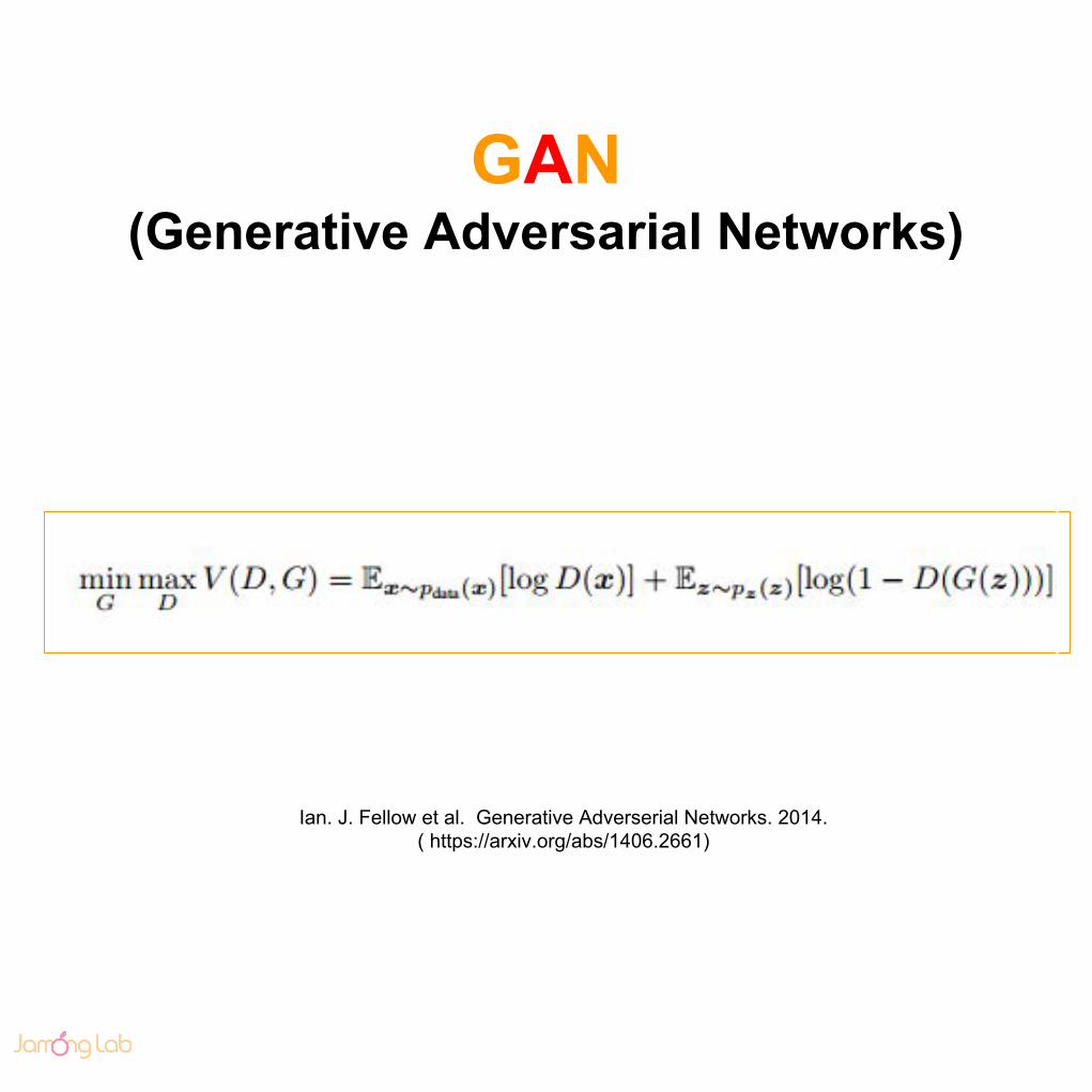
GAN(Generative Adversarial Networks)
Ian. J. Fellow et al. Generative Adverserial Networks. 2014. ( https://arxiv.org/abs/1406.2661)

Discriminator

Generator

Adversarial Network
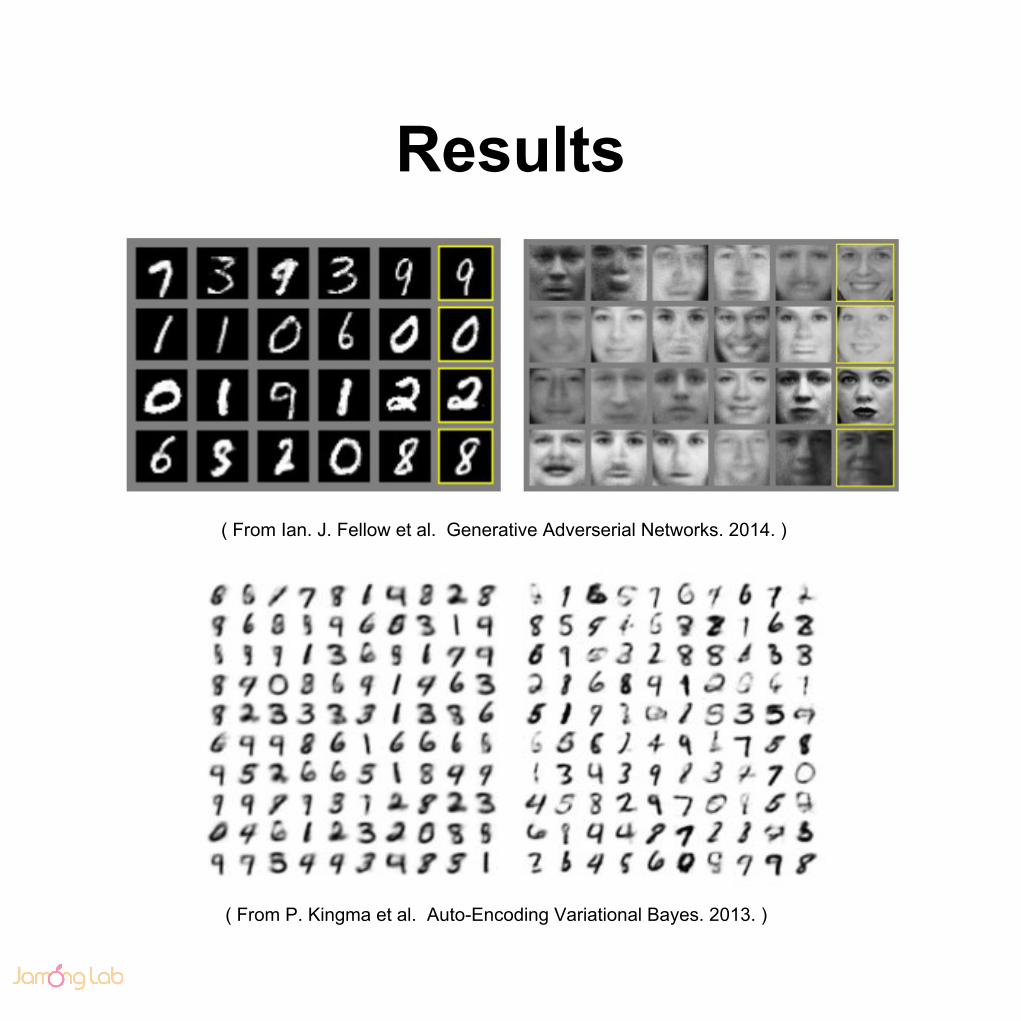
Results
( From Ian. J. Fellow et al. Generative Adverserial Networks. 2014. )
( From P. Kingma et al. Auto-Encoding Variational Bayes. 2013. )

Pitfalls of GAN
● Very difficult to train.
○ No guarantee to Nash Equilibrium.■ Tim Salimans et al, Improved Techniques for Training GANS, 2016.
■ Junbo Zhao et al, Energy-based Generative Adversarial Network,
2016.
● Cannot control generated data.
○ How can we condition generating
function G(x)?

InfoGAN
Xi Chen et al. InfoGAN: Interpretable Representation Learning by Information Maximizing Generative Adversarial Nets, 2016 ( https://arxiv.org/abs/1606.03657 )
● Add mutual Information regularizer for inducing latent codes to original GAN.

InfoGAN

Results
( From Xi Chen et al. InfoGAN: Interpretable Representation Learning by Information Maximizing Generative Adversarial Nets)

Results
Interpretable factors interfered on face dataset

Supervised InfoGAN

Results
(From https://github.com/buriburisuri/supervised_infogan)

AC-GAN● Augustus, “Conditional Image Synthesis With Auxiliary Classifier GANs”,
2016

Features of GAN
● Unsupervised
○ No labelled data used
● End-to-end
○ No human feature engineering
○ No prior nor assumption
● High fidelity
○ automatic highly non-linear pattern finding
⇒ Currently, SOTA in image generation.

Skipped topics
● Ensemble & Distillation
● Attention + RNN
● Object Tracking
● And so many ...
Computers have opened their eyes.

Thanks