convex optimization in signal processing and … constrained optimization problem obtained by...
TRANSCRIPT

Convex Optimization in SignalProcessing and Communications
March 20, 2009
i

ii
Contents
List of contributors page iv
Part I 1
1 Cooperative Distributed Multi-Agent Optimization 31.1 Introduction and Motivation 31.2 Distributed Optimization Methods using Dual Decomposition 6
1.2.1 Basic Notation and Terminology 61.2.2 Primal and Dual Problem 71.2.3 Distributed Methods for Utility-based Network Resource Allo-
cation 111.2.4 Approximate Primal Solutions and Rate Analysis 131.2.5 Numerical Example 19
1.3 Distributed Optimization Methods using Consensus Algorithms 201.3.1 Problem and Algorithm 221.3.2 Information Exchange Model 241.3.3 Convergence of Transition Matrices 261.3.4 Convergence Analysis of the Subgradient Method 28
1.4 Extensions 351.4.1 Quantization Effects on Optimization 351.4.2 Consensus with Local Constraints 37
1.5 Future Work 401.5.1 Optimization with Delays 411.5.2 Optimization with Constraints 421.5.3 Nonconvex Local Objective Functions 43
1.6 Conclusions 431.7 Problems 44
References 47Index 50
iii

List of contributors
Angelia Nedic
Angelia Nedic received her B.S. degree from the University of Montenegro in 1987and M.S. degree from the University of Belgrade in 1990, both in Mathematics.She received her Ph.D. degrees from Moscow State University in 1994 in Math-ematics and Mathematical Physics, and from Massachusetts Institute of Tech-nology in Electrical Engineering and Computer Science in 2002. She has been atthe BAE Systems Advanced Information Technology from 2002-2006. Since 2006she has been an Assistant Professor at the Department of Industrial and Enter-prise Systems Engineering at the University of Illinois at Urbana-Champaign.Her general interest is in optimization including fundamental theory, models,algorithms, and applications.
Asuman Ozdaglar
Asuman Ozdaglar is the Class of 1943 Associate Professor in the Electrical Engi-neering and Computer Science Department at the Massachusetts Institute ofTechnology. She is also a member of the Laboratory for Information and Deci-sion Systems and the Operations Research Center. She received the B.S. degreein electrical engineering from the Middle East Technical University, Ankara,Turkey, in 1996, and the S.M. and the Ph.D. degrees in electrical engineering andcomputer science from the Massachusetts Institute of Technology, Cambridge, in1998 and 2003, respectively. Her research interests include optimization theory,with emphasis on nonlinear programming and convex analysis, game theory, withapplications in communication, social, and economic networks, and distributedoptimization methods.
iv

Part I
1

2
1 Cooperative DistributedMulti-Agent Optimization
Angelia Nedic and Asuman Ozdaglar
Angelia Nedic is with the University of Illinois at Urbana-Champaign.Asuman Ozdaglar is with the Massachusetts Institute of Technology.
This chapter presents distributed algorithms for cooperative optimization amongmultiple agents connected through a network. The goal is to optimize a globalobjective function which is a combination of local objective functions known bythe agents only. We focus on two related approaches for the design of distributedalgorithms for this problem. The first approach relies on using Lagrangian decom-position and dual subgradient methods. We show that this methodology leads todistributed algorithms for optimization problems with special structure. The sec-ond approach involves combining consensus algorithms with subgradient meth-ods. In both approaches, our focus is on providing convergence rate analysis forthe generated solutions that highlight the dependence on problem parameters.
1.1 Introduction and Motivation
There has been much recent interest in distributed control and coordination ofnetworks consisting of multiple agents, where the goal is to collectively opti-mize a global objective. This is motivated mainly by the emergence of largescale networks and new networking applications such as mobile ad hoc networksand wireless sensor networks, characterized by the lack of centralized access toinformation and time-varying connectivity. Control and optimization algorithmsdeployed in such networks should be completely distributed, relying only on localobservations and information, robust against unexpected changes in topology,such as link or node failures, and scalable in the size of the network.
This chapter studies the problem of distributed optimization and control ofmulti-agent networked systems. More formally, we consider a multi-agent net-work model, where m agents exchange information over a connected network.Each agent i has a local convex objective function fi(x), with fi : Rn → R, anda nonempty local convex constraint set Xi, with Xi ⊂ Rn, known by this agentonly. The vector x ∈ Rn represents a global decision vector that the agents arecollectively trying to decide on.
The goal of the agents is to cooperatively optimize a global objective function,denoted by f(x), which is a combination of the local objective functions, i.e.,
f(x) = T(f1(x), . . . , fm(x)
),
3

4 Chapter 1. Cooperative Distributed Multi-Agent Optimization
Figure 1.1 Multiagent cooperative optimization problem.
where T : Rm → R is an increasing convex function.1 The decision vector x isconstrained to lie in a set, x ∈ C, which is a combination of local constraints andadditional global constraints that may be imposed by the network structure, i.e.,
C =(∩m
i=1 Xi
)∩ Cg,
where Cg represents the global constraints. This model leads to the followingoptimization problem:
minimize f(x) (1.1)
subject to x ∈ C,
where the function f : Rn → R is a convex objective function and the set C is aconvex constraint set (see Figure 1.1). The decision vector x in problem (1.1) canbe viewed as either a resource vector whose components correspond to resourcesallocated to each agent, or a global parameter vector to be estimated by theagents using local information.
Our goal in this chapter is to develop optimization methods that the agentscan use to solve problem (1.1) within the informational structure available tothem. Our development relies on using first-order methods, i.e., gradient-basedmethods (or subgradient methods for the case when the local objective functions
1 By an increasing function, we mean for any w, y ∈ Rm with w ≥ y with respect to the usualvector order (i.e., the inequality holds componentwise), we have T (w) ≥ T (y).

Cooperative Distributed Multi-Agent Optimization 5
fi are nonsmooth). Due to simplicity of computations per iteration, first-ordermethods have gained popularity in the last few years as low overhead alternativesto interior-point methods, that may lend themselves to distributed implemen-tations. Despite the fact that first-order methods have slower convergence rate(compared to interior point methods) in finding high-accuracy solutions, theyare particularly effective in large scale multi-agent optimization problems wherethe goal is to generate near-optimal approximate solutions in relatively smallnumber of iterations.
This chapter will present both classical results and recent advances on thedesign and analysis of distributed optimization algorithms. The theoretical devel-opment will be complemented with recent application areas for these methods.Our development will focus on two major methodologies.
The first approach relies on using Lagrangian dual decomposition and dualmethods for solving problem (1.1). We will show that this approach leads to dis-tributed optimization algorithms when problem (1.1) is separable (i.e., problemswhere local objective functions and constraints decompose over the componentsof the decision vector). This methodology has been used extensively in the net-working literature to design cross-layer resource allocation mechanisms (see [23],[27], [48], [50], and [14]). Our focus in this chapter will be on generating approxi-mate (primal) solutions from the dual algorithm and providing convergence rateestimates. Despite the fact that duality yields distributed methods primarily forseparable problems, our methods and rate analysis are applicable for generalconvex problems and will be covered here in their general version.
When problem (1.1) is not separable, dual decomposition approach will notlead to distributed methods. For such problems, we present optimization meth-ods that use consensus algorithms as a building block. Consensus algorithmsinvolve each agent maintaining estimates of the decision vector x and updatingit based on local information that becomes available through the communicationnetwork. These algorithms have attracted much attention in the cooperative con-trol literature for distributed coordination of a system of dynamic agents (see[6] [7], [8], [9], [10] [11] [12], [13], [20], [21], [22], [29], [44] [45], [46] [54], [55]).These works mainly focus on the canonical consensus problem, where the goal isto design distributed algorithms that can be used by a group of agents to agreeon a common value. Here, we show that consensus algorithms can be combinedwith first-order methods to design distributed methods that can optimize generalconvex local objective functions over a time-varying network topology.
The chapter is organized into four sections. In Section 1.2, we present dis-tributed algorithms designed using Lagrangian duality and subgradient meth-ods. We show that for (separable) network resource allocation problems, thismethodology yields distributed optimization methods. We present recent resultson generating approximate primal solutions from dual subgradient methods andprovide convergence rate analysis. In Section 1.3, we develop distributed meth-ods for optimizing the sum of general (non-separable) convex objective functions

6 Chapter 1. Cooperative Distributed Multi-Agent Optimization
corresponding to multiple agents connected over a time-varying topology. Thesemethods will involve a combination of first-order methods and consensus algo-rithms. Section 1.4 focuses on extensions of the distributed methods to handlelocal constraints and imperfections associated with implementing optimizationalgorithms over networked systems, such as delays, asynchronism, and quanti-zation effects, and studies the implications of these considerations on the net-work algorithm performance. Section 1.5 suggests a number of areas for futureresearch.
1.2 Distributed Optimization Methods using Dual Decomposition
This section focuses on subgradient methods for solving the dual problem of aconvex constrained optimization problem obtained by Lagrangian relaxation ofsome of the constraints. For separable problems, this method leads to decompo-sition of the computations at each iteration into subproblems that each agentcan solve using his local information and the prices (or dual variables).
In the first part of the section, we formally define the dual problem of a (primal)convex constrained optimization problem. We establish relations between the pri-mal and the dual optimal values, and investigate properties of the dual optimalsolution set. In Section 1.2.3, we introduce the utility-based network resourceallocation problem and show that Lagrangian decomposition and dual subgra-dient methods yield distributed optimization methods for solving this problem.Since the main interest in most practical applications is to obtain near-optimalsolutions to problem (1.1), the remainder of the section focuses on obtainingapproximate primal solutions using information directly available from dual sub-gradient methods and presents the corresponding rate analysis.
We start by defining the basic notation and terminology used throughout thechapter.
1.2.1 Basic Notation and Terminology
We consider the n-dimensional vector space Rn and the m-dimensional vectorspace Rm. We view a vector as a column vector, and we denote by x′y the innerproduct of two vectors x and y. We use ‖y‖ to denote the standard Euclideannorm, ‖y‖ =
√y′y. We write dist(y, Y ) to denote the standard Euclidean distance
of a vector y from a set Y , i.e.,
dist(y, Y ) = infy∈Y
‖y − y‖.
For a vector u ∈ Rm, we write u+ to denote the projection of u on the nonnegativeorthant in Rm, i.e., u+ is the component-wise maximum of the vector u and thezero vector:
u+ = (max{0, u1}, · · · , max{0, um})′ for u = (u1, · · · , um)′.

Cooperative Distributed Multi-Agent Optimization 7
For a convex function F : Rn → [−∞,∞], we denote the domain of F bydom(F ), where
dom(F ) = {x ∈ Rn | F (x) < ∞}.We use the notion of a subgradient of a convex function F (x) at a given vectorx ∈ dom(F ). A subgradient sF (x) of a convex function F (x) at any x ∈ dom(F )provides a linear underestimate of the function F . In particular, sF (x) ∈ Rn is asubgradient of a convex function F : Rn → R at a given vector x ∈ dom(F ) whenthe following relation holds:
F (x) + sF (x)′(x− x) ≤ F (x) for all x ∈ dom(F ). (1.2)
The set of all subgradients of F at x is denoted by ∂F (x).Similarly, for a concave function q : Rm → [−∞,∞], we denote the domain of
q by dom(q), where
dom(q) = {µ ∈ Rm | q(µ) > −∞}.A subgradient of a concave function is defined through a subgradient of a convexfunction −q(µ). In particular, sq(µ) ∈ Rm is a subgradient of a concave functionq(µ) at a given vector µ ∈ dom(q) when the following relation holds:
q(µ) + sq(µ)′(µ− µ) ≥ q(µ) for all µ ∈ dom(q). (1.3)
The set of all subgradients of q at µ is denoted by ∂q(µ).
1.2.2 Primal and Dual Problem
We consider the following constrained optimization problem:
minimize f(x) (1.4)
subject to g(x) ≤ 0
x ∈ X,
where f : Rn → R is a convex function, g = (g1, . . . , gm)′ and each gj : Rn → Ris a convex function, and X ⊂ Rn is a nonempty closed convex set. We refer toproblem (1.4) as the primal problem . We denote the primal optimal value by f ∗
and the primal optimal set by X∗. Throughout this section, we assume that thevalue f ∗ is finite.
We next define the dual problem for problem (1.4). The dual problem isobtained by first relaxing the inequality constraints g(x) ≤ 0 in problem (1.4),which yields the dual function q : Rm → R given by
q(µ) = infx∈X
{f(x) + µ′g(x)}. (1.5)

8 Chapter 1. Cooperative Distributed Multi-Agent Optimization
The dual problem is then given by
maximize q(µ) (1.6)
subject to µ ≥ 0
µ ∈ Rm.
We denote the dual optimal value by q∗ and the dual optimal set by M ∗.The primal and the dual problem can be visualized geometrically by consid-
ering the set V of constraint-cost function values as x ranges over the set X,i.e.,
V = {(g(x), f(x)) | x ∈ X},(see Figure 1.2). In this figure, the primal optimal value f ∗ corresponds to theminimum vertical axis value of all points on the left-half plane, i.e., all points ofthe form {g(x) ≤ 0 | x ∈ X}. Similarly, for a given dual feasible solution µ ≥ 0,the dual function value q(µ) corresponds to the vertical intercept value of allhyperplanes with normal (µ, 1) and support the set V from below.2 The dualoptimal value q∗ then corresponds to the maximum intercept value of such hyper-planes over all µ ≥ 0 [see Figure 1.2(b)]. This figure provides much insight aboutthe relation between the primal and the dual problems and the structure of dualoptimal solutions, and has been used recently to develop a duality theory basedon geometric principles (see [2] for convex constrained optimization problems,and [36, 37, 42] for nonconvex constrained optimization problems).
Duality Gap and Dual SolutionsIt is clear from the geometric picture that the primal and dual optimal valuessatisfy q∗ ≤ f ∗, which is the well-known weak duality relation (see Bertsekas etal. [4]). When f ∗ = q∗, we say that there is no duality gap or strong duality holds.The next condition guarantees that there is no duality gap.
Assumption 1. (Slater Condition) There exists a vector x ∈ X such that
gj(x) < 0 for all j = 1, . . . ,m.
We refer to a vector x satisfying the Slater condition as a Slater vector.
2 A hyperplane H ⊂ Rn is an (n− 1)-dimensional affine set, which is defined through itsnonzero normal vector a ∈ Rn and a scalar b as
H = {x ∈ Rn | a′x = b}.Any vector x ∈ H can be used to determine the constant b as a′x = b, thus yielding anequivalent representation of the hyperplane H as
H = {x ∈ Rn | a′x = a′x}.Here, we consider hyperplanes in Rr+1 with normal vectors given by (µ, 1) ∈ Rr+1.

Cooperative Distributed Multi-Agent Optimization 9
Figure 1.2 Illustration of the primal and the dual problem.
Under the convexity assumptions on the primal problem (1.4) and the assump-tion that f ∗ is finite, it is well-known that the Slater condition is sufficient for noduality gap as well as for the existence of a dual optimal solution (see for exampleBertsekas [3] or Bertsekas et. al [4]). Furthermore, under Slater condition, thedual optimal set is bounded (see Uzawa [53] and Hiriart-Urruty and Lemarechal[19]). Figure 1.3 provides some intuition for the role of convexity and the Slatercondition in establishing no duality gap and the boundedness of the dual optimalsolution set.
The following lemma extends the result on the optimal dual set boundednessunder the Slater condition. In particular, it shows that the Slater condition alsoguarantees the boundedness of the (level) sets {µ ≥ 0 | q(µ) ≥ q(µ)}.
Lemma 1.1. Let the Slater condition hold [cf. Assumption 1]. Then, the setQµ = {µ ≥ 0 | q(µ) ≥ q(µ)} is bounded and, in particular, we have
maxµ∈Qµ
‖µ‖ ≤ 1γ
(f(x)− q(µ)) ,
where γ = min1≤j≤m{−gj(x)} and x is a Slater vector.
Proof. We have for any µ ∈ Qµ,
q(µ) ≤ q(µ) = infx∈X
{f(x) + µ′g(x)} ≤ f(x) + µ′g(x) = f(x) +m∑
j=1
µjgj(x),

10 Chapter 1. Cooperative Distributed Multi-Agent Optimization
Figure 1.3 Parts (a) and (b) provide two examples where there is a duality gap [due tolack of convexity in (a) and lack of “continuity around origin” in (b)]. Part (c)illustrates the role of the Slater condition in establishing no duality gap andboundedness of the dual optimal solutions. Note that dual optimal solutionscorrespond to the normal vectors of the (nonvertical) hyperplanes supporting set Vfrom below at the point (0, q∗).
implying that
−m∑
j=1
µjgj(x) ≤ f(x)− q(µ).
Because gj(x) < 0 and µj ≥ 0 for all j, it follows that
min1≤j≤m
{−gj(x)}m∑
j=1
µj ≤ −m∑
j=1
µjgj(x) ≤ f(x)− q(µ).
Therefore,m∑
j=1
µj ≤ f(x)− q(µ)min1≤j≤m {−gj(x)} .
Since µ ≥ 0, we have ‖µ‖ ≤ ∑mj=1 µj and the estimate follows. Q.E.D.

Cooperative Distributed Multi-Agent Optimization 11
It can be seen from the preceding lemma that under the Slater condition, thedual optimal set M ∗ is nonempty. In particular, by noting that M ∗ = {µ ≥ 0 |q(µ) ≥ q∗} and by using Lemma 1.1, we see that
maxµ∗∈M∗
‖µ∗‖ ≤ 1γ
(f(x)− q∗) , (1.7)
with γ = min1≤j≤m{−gj(x)}.
Dual Subgradient MethodSince the dual function q(µ) given by Eq. (1.5) is the infimum of a collection ofaffine functions, it is a concave function (see [4]). Hence, we can use a subgradientmethod to solve the dual problem (1.6). In view of its implementation simplicity,we consider the classical subgradient algorithm with a constant stepsize:
µk+1 = [µk + αgk]+ for k = 0, 1, . . . , (1.8)
where the vector µ0 ≥ 0 is an initial iterate, the scalar α > 0 is a stepsize, andthe vector gk is a subgradient of q at µk. Due to the form of the dual function q,the subgradients of q at a vector µ are related to the primal vectors xµ attainingthe minimum in Eq. (1.5). Specifically, the set ∂q(µ) of subgradients of q at agiven µ ≥ 0 is given by
∂q(µ) = conv ({g(xµ) | xµ ∈ Xµ}) , Xµ = {xµ ∈ X | q(µ) = f(xµ) + µ′g(xµ)},(1.9)
where conv(Y ) denotes the convex hull of a set Y (see [4]).
1.2.3 Distributed Methods for Utility-based Network Resource Allocation
In this section, we consider a utility-based network resource allocation prob-lem and briefly discuss how dual decomposition and subgradient methods leadto decentralized optimization methods that can be used over a network. Thisapproach was proposed in the seminal work of Kelly [23] and further developedby Low and Lapsley [27], Shakkottai and Srikant [48], and Srikant [50].
Consider a network that consists of a set S = {1, . . . , S} of sources and a setL = {1, . . . , L} of undirected links, where a link l has capacity cl. Let L(i) ⊂ Ldenote the set of links used by source i. The application requirements of sourcei is represented by a concave increasing utility function ui : [0,∞) → [0,∞),i.e., each source i gains a utility ui(xi) when it sends data at a rate xi. Wefurther assume that rate xi is constrained to lie in the interval Ii = [0,Mi] forall i ∈ S, where the scalar Mi denotes the maximum allowed rate for source i.Let S(l) = {i ∈ S | l ∈ L(i)} denote the set of sources that use link l. The goalof the network utility maximization problem is to allocate the source rates as the

12 Chapter 1. Cooperative Distributed Multi-Agent Optimization
optimal solution of the problem
maximize∑
i∈Sui(xi) (1.10)
subject to∑
i∈S(l)
xi ≤ cl for all l ∈ L (1.11)
xi ∈ Ii for all i ∈ S.
This problem is a special case of the multi-agent optimization problem (1.1),where the local objective function of each agent (or source) fi(x) is given byfi(x) = −ui(xi), i.e., the local objective function of each agent depends only onone component of the decision vector x and the overall objective function f(x)is the sum of the local objective functions, f(x) = −∑
i ui(xi), i.e., the globalobjective function f(x) is separable in the components of the decision vector.Moreover, the global constraint set Cg is given by the link capacity constraints(1.11), and the local constraint set of each agent Xi is given by the intervalIi. Note that only agent i knows his utility function ui(xi) and his maximumallowed rate Mi, which specifies the local constraint xi ∈ Ii.
Solving problem (1.10) directly by applying existing subgradient methodsrequires coordination among sources and therefore may be impractical for realnetworks. This is in view of the fact that in large-scale networks, such as the Inter-net, there is no central entity that has access to both the source utility functionsand constraints, and the capacity of all the links in the network. Despite thisinformation structure, in view of the separable structure of the objective andconstraint functions, the dual problem can be evaluated exactly using decen-tralized information. In particular, the dual problem of (1.10) is given by (1.6),where the dual function takes the form
q(µ) = maxxi∈Ii, i∈S
∑
i∈Sui(xi)−
∑
l∈Lµl
( ∑
i∈S(l)
xi − cl
)
= maxxi∈Ii, i∈S
∑
i∈S
(ui(xi)− xi
∑
l∈L(i)
µl
)+
∑
l∈Lµlcl.
Since the optimization problem on the right-hand side of the preceding relation isseparable in the variables xi, the problem decomposes into subproblems for eachsource i. Letting µi =
∑l∈L(i) µl for each i (i.e., µi is the sum of the multipliers
corresponding to the links used by source i), we can write the dual function as
q(µ) =∑
i∈Smaxxi∈Ii
{ui(xi)− xiµi}+∑
l∈Lµlcl.
Hence, to evaluate the dual function, each source i needs to solve the one-dimensional optimization problem maxxi∈Ii
{ui(xi)− xiµi}. This involves onlyits own utility function ui and the value µi, which is available to source i inpractical networks (through a direct feedback mechanism from its destination).
Using a subgradient method to solve the dual problem (1.6) yields the follow-ing distributed optimization method, where at each iteration k ≥ 0, links and

Cooperative Distributed Multi-Agent Optimization 13
sources update their prices (or dual solution values) and rates respectively in adecentralized manner:Link Price Update: Each link l updates its price µl according to
µl(k + 1) = [µl(k) + αgl(k)]+,
where gl(k) =∑
i∈S(l) xi(k)− cl, i.e., gl(k) is the value of the link l capacityconstraint (1.11) at the primal vector x(k) [see the relation for the subgradientof the dual function q(µ) in Eq. (1.9)].Source Rate Update: Each source i updates its rate xi according to
xi(k + 1) = arg maxxi∈Ii
{ui(xi)− xiµi}.
The preceding methodology has motivated much interest in using dual decom-position and subgradient methods to solve network resource allocation problemsin an iterative decentralized manner (see Chiang et. al [14]). Other problemswhere the dual problem has a structure that allows exact evaluation of the dualfunction using local information include the problem of processor speed controlconsidered by Mutapcic et. al [30], and the traffic equilibrium and road pricingproblems considered by Larsson et. al [24], [25], [26].
1.2.4 Approximate Primal Solutions and Rate Analysis
We first establish some basic relations that hold for a sequence {µk} obtainedby the subgradient algorithm of Eq. (1.8).
Lemma 1.2. Let the sequence {µk} be generated by the subgradient algorithm(1.8). For any µ ≥ 0, we have
‖µk+1 − µ‖2 ≤ ‖µk − µ‖2 − 2α (q(µ)− q(µk)) + α2‖gk‖2 for all k ≥ 0.
Proof. By using the nonexpansive property of the projection operation, fromrelation (1.8) we obtain for any µ ≥ 0 and all k,
‖µk+1 − µ‖2 =∥∥[µk + αgk]+ − µ
∥∥2 ≤ ‖µk + αgk − µ‖2 .
Therefore,
‖µk+1 − µ‖2 ≤ ‖µk − µ‖2 + 2αg′k(µk − µ) + α2‖gk‖2 for all k.
Since gk is a subgradient of q at µk [cf. Eq. (1.3)], we have
g′k(µ− µk) ≥ q(µ)− q(µk),
implying that
g′k(µk − µ) ≤ − (q(µ)− q(µk)) .

14 Chapter 1. Cooperative Distributed Multi-Agent Optimization
Hence, for any µ ≥ 0,
‖µk+1 − µ‖2 ≤ ‖µk − µ‖2 − 2α (q(µ)− q(µk)) + α2‖gk‖2 for all k.
Q.E.D.
Boundedness of Dual IteratesHere, we show that the dual sequence {µk} generated by the subgradient algo-rithm is bounded under the Slater condition and a boundedness assumption onthe subgradient sequence {gk}. We formally state the latter requirement in thefollowing.
Assumption 2. (Bounded Subgradients) The subgradient sequence {gk} isbounded, i.e., there exists a scalar L > 0 such that
‖gk‖ ≤ L for all k ≥ 0.
This assumption is satisfied, for example, when the primal constraint set X iscompact. Due to the convexity of the constraint functions gj over Rn, each gj iscontinuous over Rn. Thus, maxx∈X ‖g(x)‖ is finite and provides an upper boundon the norms of the subgradients gk, i.e.,
‖gk‖ ≤ L for all k ≥ 0, with L = maxx∈X
‖g(x)‖.
In the following lemma, we establish the boundedness of the dual sequencegenerated by the subgradient method.
Lemma 1.3. Let the dual sequence {µk} be generated by the subgradient algo-rithm of Eq. (1.8). Also, let the Slater condition and the Bounded Subgradientsassumption hold [cf. Assumptions 1 and 2]. Then, the sequence {µk} is boundedand, in particular, we have
‖µk‖ ≤ 2γ
(f(x)− q∗) + max{‖µ0‖, 1
γ(f(x)− q∗) +
αL2
2γ+ αL
},
where γ = min1≤j≤m{−gj(x)}, x is a Slater vector, L is the subgradient normbound, and α > 0 is the stepsize.
Proof. Under the Slater condition the optimal dual set M ∗ is nonempty. Considerthe set Qα defined by
Qα ={
µ ≥ 0 | q(µ) ≥ q∗ − αL2
2
},
which is nonempty in view of M ∗ ⊂ Qα. We fix an arbitrary µ∗ ∈ M ∗ and wefirst prove that for all k ≥ 0,
‖µk − µ∗‖ ≤ max{‖µ0 − µ∗‖, 1
γ(f(x)− q∗) +
αL2
2γ+ ‖µ∗‖+ αL
}, (1.12)

Cooperative Distributed Multi-Agent Optimization 15
where γ = min1≤j≤m{−gj(x)} and L is the bound on the subgradient norms‖gk‖. Then, we use Lemma 1.1 to prove the desired estimate.
We show that relation (1.12) holds by induction on k. Note that the relationholds for k = 0. Assume now that it holds for some k > 0, i.e.,
‖µk − µ∗‖ ≤ max{‖µ0 − µ∗‖, 1
γ(f(x)− q∗) +
αL2
2γ+ ‖µ∗‖+ αL
}for some k > 0.
(1.13)We now consider two cases: q(µk) ≥ q∗ − αL2/2 and q(µk) < q∗ − αL2/2.
Case 1: q(µk) ≥ q∗ − αL2/2. By using the definition of the iterate µk+1 in Eq.(1.8) and the subgradient boundedness, we obtain
‖µk+1 − µ∗‖ ≤ ‖µk + αgk − µ∗‖ ≤ ‖µk‖+ ‖µ∗‖+ αL.
Since q(µk) ≥ q∗ − αL2/2, it follows that µk ∈ Qα. According to Lemma 1.1,the set Qα is bounded and, in particular, ‖µ‖ ≤ 1
γ
(f(x)− q∗ + αL2/2
)for all
µ ∈ Qα. Therefore
‖µk‖ ≤ 1γ
(f(x)− q∗) +αL2
2γ.
By combining the preceding two relations, we obtain
‖µk+1 − µ∗‖ ≤ 1γ
(f(x)− q∗) +αL2
2γ+ ‖µ∗‖+ αL,
thus showing that the estimate in Eq. (1.12) holds for k + 1.
Case 2: q(µk) < q∗ − αL2/2. By using Lemma 1.2 with µ = µ∗, we obtain
‖µk+1 − µ∗‖2 ≤ ‖µk − µ∗‖2 − 2α (q∗ − q(µk)) + α2‖gk‖2.By using the subgradient boundedness, we further obtain
‖µk+1 − µ∗‖2 ≤ ‖µk − µ∗‖2 − 2α
(q∗ − q(µk)− αL2
2
).
Since q(µk) < q∗ − αL2/2, it follows that q∗ − q(µk)− αL2/2 > 0, which whencombined with the preceding relation yields
‖µk+1 − µ∗‖ < ‖µk − µ∗‖.By the induction hypothesis [cf. Eq. (1.13)], it follows that the estimate in Eq.(1.12) holds for k + 1 as well. Hence, the estimate in Eq. (1.12) holds for allk ≥ 0.
From Eq. (1.12) we obtain for all k ≥ 0,
‖µk‖ ≤ ‖µk − µ∗‖+ ‖µ∗‖≤ max
{‖µ0 − µ∗‖, 1
γ(f(x)− q∗) +
αL2
2γ+ ‖µ∗‖+ αL
}+ ‖µ∗‖.

16 Chapter 1. Cooperative Distributed Multi-Agent Optimization
By using ‖µ0 − µ∗‖ ≤ ‖µ0‖+ ‖µ∗‖, we further have for all k ≥ 0,
‖µk‖ ≤ max{‖µ0‖+ ‖µ∗‖, 1
γ(f(x)− q∗) +
αL2
2γ+ ‖µ∗‖+ αL
}+ ‖µ∗‖
= 2‖µ∗‖+ max{‖µ0‖, 1
γ(f(x)− q∗) +
αL2
2γ+ αL
}.
Since M ∗ = {µ ≥ 0 | q(µ) ≥ q∗}, according to Lemma 1.1, we have the followingbound on the dual optimal solutions
maxµ∗∈M∗
‖µ∗‖ ≤ 1γ
(f(x)− q∗) ,
implying that for all k ≥ 0,
‖µk‖ ≤ 2γ
(f(x)− q∗) + max{‖µ0‖, 1
γ(f(x)− q∗) +
αL2
2γ+ αL
}.
Q.E.D.
Convergence Rate EstimatesIn this section, we generate approximate primal solutions by considering therunning averages of the primal sequence {xk} obtained in the implementationof the subgradient method. We show that under the Slater condition, we canprovide bounds for the number of subgradient iterations needed to generate aprimal solution within a given level of constraint violation. We also derive upperand lower bounds on the gap from the optimal primal value.
To define the approximate primal solutions, we consider the dual sequence{µk} generated by the subgradient algorithm in (1.8), and the correspondingsequence of primal vectors {xk} ⊂ X that provide the subgradients gk in thealgorithm , i.e.,
gk = g(xk), xk ∈ arg minx∈X
{f(x) + µ′kg(x)} for all k ≥ 0, (1.14)
[see the subdifferential relation in (1.9)]. We define xk as the average of thevectors x0, . . . , xk−1, i.e.,
xk =1k
k−1∑
i=0
xi for all k ≥ 1. (1.15)
The average vectors xk lie in the set X because X is convex and xi ∈ X forall i. However, these vectors need not satisfy the primal inequality constraintsgj(x) ≤ 0, j = 1, . . . , m, and therefore, they can be primal infeasible.
The next proposition provides a bound on the amount of feasibility violationof the running averages xk. It also provides upper and lower bounds on theprimal cost of these vectors. These bounds are given per iteration, as seen in thefollowing.

Cooperative Distributed Multi-Agent Optimization 17
Theorem 1.1. Let the sequence {µk} be generated by the subgradient algo-rithm (1.8). Let the Slater condition and Bounded Subgradients assumption hold[cf. Assumptions 1 and 2]. Also, let
B∗ =2γ
(f(x)− q∗) + max{‖µ0‖, 1
γ(f(x)− q∗) +
αL2
2γ+ αL
}. (1.16)
Let the vectors xk for k ≥ 1 be the averages given by Eq. (1.15). Then, thefollowing holds for all k ≥ 1:
(a) An upper bound on the amount of constraint violation of the vector xk isgiven by
‖g(xk)+‖ ≤ B∗
kα.
(b) An upper bound on the primal cost of the vector xk is given by
f(xk) ≤ f ∗ +‖µ0‖22kα
+αL2
2.
(c) A lower bound on the primal cost of the vector xk is given by
f(xk) ≥ f ∗ − 1γ
[ f(x)− q∗ ] ‖g(xk)+‖.
Proof. (a) By using the definition of the iterate µk+1 in Eq. (1.8), we obtain
µk + αgk ≤ [µk + αgk]+ = µk+1 for all k ≥ 0.
Since gk = g(xk) with xk ∈ X, it follows that
αg(xk) ≤ µk+1 − µk for all k ≥ 0.
Therefore,k−1∑
i=0
αg(xi) ≤ µk − µ0 ≤ µk for all k ≥ 1,
where the last inequality in the preceding relation follows from µ0 ≥ 0. Sincexk ∈ X for all k, by the convexity of X, we have xk ∈ X for all k. Hence, by theconvexity of each of the functions gj , it follows that
g(xk) ≤ 1k
k−1∑
i=0
g(xi) =1
kα
k−1∑
i=0
αg(xi) ≤ µk
kαfor all k ≥ 1.
Because µk ≥ 0 for all k, we have g(xk)+ ≤ µk/(kα) for all k ≥ 1 and, therefore,
∥∥g(xk)+∥∥ ≤ ‖µk‖
kαfor all k ≥ 1. (1.17)
By Lemma 1.3 we have
‖µk‖ ≤ 2γ
(f(x)− q∗) + max{‖µ0‖, 1
γ(f(x)− q∗) +
αL2
2γ+ αL
}for all k ≥ 0.

18 Chapter 1. Cooperative Distributed Multi-Agent Optimization
By the definition of B∗ in Eq. (1.16), the preceding relation is equivalent to
‖µk‖ ≤ B∗ for all k ≥ 0.
Combining this relation with Eq. (1.17), we obtain
‖g(xk)+‖ ≤ ‖µk‖kα
≤ B∗
kαfor all k ≥ 1.
(b) By the convexity of the primal cost f(x) and the definition of xk as aminimizer of the Lagrangian function f(x) + µ′kg(x) over x ∈ X [cf. Eq. (1.14)],we have
f(xk) ≤ 1k
k−1∑
i=0
f(xi) =1k
k−1∑
i=0
{f(xi) + µ′ig(xi)} − 1k
k−1∑
i=0
µ′ig(xi).
Since q(µi) = f(xi) + µ′ig(xi) and q(µi) ≤ q∗ for all i, it follows that for all k ≥ 1,
f(xk) ≤ 1k
k−1∑
i=0
q(µi)− 1k
k−1∑
i=0
µ′ig(xi) ≤ q∗ − 1k
k−1∑
i=0
µ′ig(xi). (1.18)
From the definition of the algorithm in Eq. (1.8), by using the nonexpansiveproperty of the projection, and the facts 0 ∈ {µ ∈ Rm | µ ≥ 0} and gi = g(xi),we obtain
‖µi+1‖2 ≤ ‖µi‖2 + 2αµ′ig(xi) + α2‖g(xi)‖2 for all i ≥ 0,
implying that
−µ′ig(xi) ≤ ‖µi‖2 − ‖µi+1‖2 + α2‖g(xi)‖22α
for all i ≥ 0.
By summing over i = 0, . . . , k − 1 for k ≥ 1, we have
−1k
k−1∑
i=0
µ′ig(xi) ≤ ‖µ0‖2 − ‖µk‖22kα
+α
2k
k−1∑
i=0
‖g(xi)‖2 for all k ≥ 1.
Combining the preceding relation and Eq. (1.18), we further have
f(xk) ≤ q∗ +‖µ0‖2 − ‖µk‖2
2kα+
α
2k
k−1∑
i=0
‖g(xi)‖2 for all k ≥ 1.
Under the Slater condition, there is zero duality gap, i.e., q∗ = f ∗. Furthermore,the subgradients are bounded by a scalar L [cf. Assumption 2], so that
f(xk) ≤ f ∗ +‖µ0‖22kα
+αL2
2for all k ≥ 1,
yielding the desired estimate.
(c) Given a dual optimal solution µ∗, we have
f(xk) = f(xk) + (µ∗)′g(xk)− (µ∗)′g(xk) ≥ q(µ∗)− (µ∗)′g(xk).

Cooperative Distributed Multi-Agent Optimization 19
Figure 1.4 A simple network with two links of capacities c1 = 1 and c2 = 2, and threeusers, each sending data at a rate xi.
Because µ∗ ≥ 0 and g(xk)+ ≥ g(xk), we further have
−(µ∗)′g(xk) ≥ −(µ∗)′g(xk)+ ≥ −‖µ∗‖‖g(xk)+‖.From the preceding two relations and the fact q(µ∗) = q∗ = f ∗ it follows that
f(xk) ≥ f ∗ − ‖µ∗‖‖g(xk)+‖.By using Lemma 1.1 with µ = µ∗, we see that the dual set is bounded and, inparticular, ‖µ∗‖ ≤ 1
γ (f(x)− q∗) for all dual optimal vectors µ∗. Hence,
f(xk) ≥ f ∗ − 1γ
[ f(x)− q∗ ] ‖g(xk)+‖ for all k ≥ 1.
Q.E.D.
1.2.5 Numerical Example
In this section, we study a numerical example to illustrate the performance ofthe dual subgradient method with primal averaging for the utility-based networkresource allocation problem described in Section 1.2.3. Consider the networkillustrated in Figure 1.4 with 2 serial links and 3 users each sending data at arate xi for i = 1, 2, 3. Link 1 has a capacity c1 = 1 and link 2 has a capacity c2 = 2.Assume that each user has an identical concave utility function ui(xi) =
√xi,
which represents the utility gained from sending rate xi. We consider allocatingrates among the users as the optimal solution of the problem
maximize∑3
i=1
√xi
subject to x1 + x2 ≤ 1, x1 + x3 ≤ 2,
xi ≥ 0, i = 1, 2, 3.
The optimal solution of this problem is x∗ = [0.2686, 0.7314, 1.7314] and the opti-mal value is f ∗ ≈ 2.7. We consider solving this problem using the dual subgradi-ent method of Eq. (1.8) (with a constant stepsize α = 1) combined with primalaveraging. In particular, when evaluating the subgradients of the dual functionin Eq. (1.14), we obtain the primal sequence {xk}. We generate the sequence{xk} as the running average of the primal sequence [cf. Eq. (1.15)].
Figure 1.5 illustrates the behavior of the sequences {xik} and {xik} for eachuser i = 1, 2, 3. As seen in this figure, for each user i, the sequences {xik} exhibit

20 Chapter 1. Cooperative Distributed Multi-Agent Optimization
10 20 30 40 500
1
2
3
4
5
6
7
8
9
10
k
x1(k)
x2(k)
x3(k)
10 20 30 40 500
1
2
3
4
5
6
7
8
9
10
k
x^
1(k)
x^
2(k)
x^
3(k)
Figure 1.5 The convergence behavior of the primal sequence {xk} (on the left) and{xk} (on the right).
oscillations whereas the average sequences {xik} converge smoothly to near-optimal solutions within 60 subgradient iterations.
Figure 1.6 illustrates the results for the constraint violation and the primalobjective value for the sequences {xk} and {xk}. The plot to the left in Figure 1.6shows the convergence behavior of the constraint violation ‖g(x)+‖ for the twosequences, i.e., ‖g(xk)+‖ and ‖g(xk)+‖. Note that the constraint violation forthe sequence {xk} oscillates within a large range while the constraint violationfor the average sequence {xk} rapidly converges to 0. The plot to the right inFigure 3 shows a similar convergence behavior for the primal objective functionvalues f(x) along the sequences {xk} and {xk}.
1.3 Distributed Optimization Methods using Consensus Algorithms
In this section, we develop distributed methods for minimizing the sum of non-separable convex functions corresponding to multiple agents connected over anetwork with time-varying topology. These methods combine first-order methodsand a consensus algorithm . The consensus part serves as a basic mechanism fordistributing the computations among the agents and allowing us to solve theproblem in a decentralized fashion.

Cooperative Distributed Multi-Agent Optimization 21
0 10 20 30 40 50 600
1
2
3
4
5
6
7
8
9
10
k
||g(x(k))||
||g(x^ (k))||
0 10 20 30 40 50 600
1
2
3
4
5
6
7
k
f(x^ (k))f(x(k))
Figure 1.6 The figure on the left shows the convergence behavior of the constraintviolation for the two primal sequences, {xk} and {xk}. Similarly, the figure on theright shows the convergence of the corresponding primal objective function values.
In contrast with the setting considered in Section 1.2.3 where each agent hasan objective function that depends only on the resource allocated to that agent,the model discussed in this section allows for the individual cost functions todepend on the entire resource allocation vector. In particular, the focus hereis on a distributed optimization problem in a network consisting of m agentsthat communicate locally. The global objective is to cooperatively minimize thecost function
∑mi=1 fi(x), where the function fi : Rn → R represents the cost
function of agent i, known by this agent only, and x ∈ Rn is a decision vector. Thedecision vector can be viewed as either a resource vector where sub-componentscorrespond to resources allocated to each agent, or a global decision vector whichthe agents are trying to compute using local information.
The approach presented here builds on the seminal work of Tsitsiklis [51](see also Tsitsiklis et al. [52], Bertsekas and Tsitsiklis [5]), who developed aframework for the analysis of distributed computation models.3 As mentionedearlier, the approach here is to use the consensus as a mechanism for distributingthe computations among the agents. The problem of reaching a consensus on aparticular scalar value, or computing exact averages of the initial values of theagents, has attracted much recent attention as natural models of cooperativebehavior in networked-systems (see Vicsek et al. [54], Jadbabaie et al. [20], Boydet al. [8], Olfati-Saber and Murray [44], Cao et al. [11], and Olshevsky andTsitsiklis [45]). Exploiting the consensus idea, recent work [40] (see also the shortpaper [33]) has proposed a distributed model for optimization over a network.
3 This framework focuses on the minimization of a (smooth) function f(x) by distributing theprocessing of the components of vector x ∈ Rn among n agents.

22 Chapter 1. Cooperative Distributed Multi-Agent Optimization
f2(x1, . . . , xn)
fm(x1, . . . , xn)
f1(x1, . . . , xn)
Figure 1.7 Illustration of the network with each agent having its local objective andcommunicating locally with its neighbors.
1.3.1 Problem and Algorithm
In this section, we formulate the problem of interest and present a distributedalgorithm for solving the problem.
ProblemWe consider the problem of optimizing the sum of convex objective functionscorresponding to m agents connected over a time-varying topology. The goal ofthe agents is to cooperatively solve the unconstrained optimization problem
minimize∑m
i=1 fi(x)subject to x ∈ Rn,
(1.19)
where each fi : Rn → R is a convex function, representing the local objectivefunction of agent i, which is known only to this agent. This problem is an uncon-strained version of the multi-agent optimization problem (1.1), where the globalobjective function f(x) is given by the sum of the individual local objectivefunctions fi(x), i.e.,
f(x) =m∑
j=1
fi(x),
(see Figure 1.7). We denote the optimal value of problem (1.19) by f ∗ and theset of optimal solutions by X∗.
To keep our discussion general, we do not assume differentiability of any ofthe functions fi. Since each fi is convex over the entire Rn, the function isdifferentiable almost everywhere (see [4] or [47]). At the points where the functionfails to be differentiable, a subgradient exists [as defined in Eq. (1.2)] and it canbe used in “the role of a gradient”.
AlgorithmWe next introduce a distributed subgradient algorithm for solving problem(1.19). The main idea of the algorithm is the use of consensus as a mechanism fordistributing the computations among the agents. In particular, each agent starts

Cooperative Distributed Multi-Agent Optimization 23
with an initial estimate xi(0) ∈ Rn and updates its estimate at discrete timestk, k = 1, 2, . . .. We denote by xi(k) the vector estimate maintained by agent i
at time tk. When updating, an agent i combines its current estimate xi with theestimates xj received from its neighboring agents j. Specifically, agent i updatesits estimates by setting
xi(k + 1) =m∑
j=1
aij(k)xj(k)− αdi(k), (1.20)
where the scalar α > 0 is a stepsize and the vector di(k) is a subgradient ofthe agent i cost function fi(x) at x = xi(k). The scalars ai1(k), . . . , aim(k) arenonnegative weights that agent i gives to the estimates x1(k), . . . , xm(k). Theseweights capture two aspects:
1. The active links (j, i) at time k. In particular, the neighbors j that communi-cate with agent i at time k, will be captured by assigning aij(k) > 0 (includingi itself). The neighbors j that do not communicate with i at time k, as wellas those that are not neighbors of i, are captured by assigning aij(k) = 0;
2. The weight that agent i gives to the estimates received from its neighbors.
When all objective functions are zero, i.e., fi(x) = 0 for all x and i, the methodin (1.20) reduces to
xi(k + 1) =m∑
j=1
aij(k)xj(k),
which is the consensus algorithm . In view of this, algorithm (1.20) can be seenas a combination of the “consensus step”
∑mj=1 aij(k)xj(k) and the subgradient
step −αdi(k). The subgradient step is taken by the agent to minimize its ownobjective fi(x), while the consensus step serves to align its decision xi with thedecisions of its neighbors. When the network is sufficiently often connected intime to ensure the proper mixing of the agents’ estimates, one would expect thatall agents have the same estimate after some time, at which point the algorithmwould start behaving as a “centralized” method. This intuition is behind theconstruction of the algorithm and also behind the analysis of its performance.
Representation using Transition MatricesIn the subsequent development, we find it useful to introduce A(k) to denotethe weight matrix [aij(k)]i,j=1,...,m. Using these matrices, we can capture theevolution of the estimates xi(k) generated by Eq. (1.20) over a window of time.In particular, we define a transition matrix Φ(k, s) for any s and k with k ≥ s,as follows:
Φ(k, s) = A(k)A(k − 1) · · ·A(s + 1)A(s).
Through the use of transition matrices, we can relate the estimate xi(k + 1) tothe estimates x1(s), . . . , xm(s) for any s ≤ k. Specifically, for the iterates gener-

24 Chapter 1. Cooperative Distributed Multi-Agent Optimization
ated by Eq. (1.20), we have for any i, and any s and k with k ≥ s,
xi(k + 1) =m∑
j=1
[Φ(k, s)]ijxj(s)− α
k−1∑r=s
m∑
j=1
[Φ(k, r + 1)]ijdj(r)− α di(k). (1.21)
As seen from the preceding relation, to study the asymptotic behavior of theestimates xi(k), we need to understand the behavior of the transition matri-ces Φ(k, s). We do this under some assumptions on the agent interactions thattranslate into some properties of transition matrices, as seen in the next section.
1.3.2 Information Exchange Model
The agent interactions and information aggregation at time k are modeledthrough the use of the matrix A(k) of agent weights aij(k). At each time k,this weight matrix captures the information flow (or the communication pat-tern) among the agents, as well as how the information is aggregated by eachagent, i.e., how much actual weight each agent i assigns to its own estimate xi(k)and the estimates xj(k) received from its neighbors.
For the proper mixing of the agent information, we need some assumptionson the weights aij(k) and the agent connectivity in time. When discussing theseassumptions, we use the notion of a stochastic vector and a stochastic matrix,defined as follows. A vector a is said to be a stochastic vector when its componentsai are nonnegative and
∑i ai = 1. A square matrix A is said to be stochastic when
each row of A is a stochastic vector, and it is said to be doubly stochastic whenboth A and its transpose A′ are stochastic matrices.
The following assumption puts conditions on the weights aij(k) in Eq. (1.20).
Assumption 3. For all k ≥ 0, the weight matrix A(k) is doubly stochastic withpositive diagonal. Additionally, there is a scalar η > 0 such that if aij(k) > 0,then aij(k) ≥ η.
The doubly stochasticity assumption on the weight matrix will guarantee thatthe function fi of every agent i receives the same weight in the long run. Thisensures that the agents optimize the sum of the functions fi as opposed to someweighted sum of these functions. The second part of the assumption states thateach agent gives significant weight to its own value and to the values of itsneighbors. This is needed to ensure that new information is aggregated into theagent system persistently in time.
We note that the lower bound η on weights in Assumption 3 need not beavailable to any of the agents. The existence of such a bound is merely used inthe analysis of the system behavior and the algorithm’s performance. Note alsothat such a bound η exists when each agent has a lower bound ηi on its ownweights aij(k), j = 1, . . . , m, in which case we can define η = min1≤i≤m ηi.

Cooperative Distributed Multi-Agent Optimization 25
The following are some examples of how to ensure in a distributed manner thatthe weight matrix A(k) satisfies Assumption 3 when the agent communicationsare bidirectional.
Example 1.1: Metropolis-based weights [55] are given by for all i and j withj 6= i,
aij(k) =
{1
1+max{ni(k),nj(k)} if j communicates with i at time k,
0 otherwise,
with ni(k) being the number of neighbors of communicating with agent i attime k. Using these, the weights aii(k) for all i = 1, . . . , m as follows
aii(k) = 1−∑
j 6=i
aij(k).
The next example can be viewed as a generalization of the Metropolis weights.
Example 1.2: Each agent i has planned weights aij(k), j = 1 . . . , m that theagent communicates to its neighbors together with the estimate xi(k), where thematrix A(k) of planned weights is a (row) stochastic matrix satisfying Assump-tion 3, except for doubly stochasticity. In particular, at time k, if agent j commu-nicates with agent i, then agent i receives xj(k) and the planned weight aji(k)from agent j. At the same time, agent j receives xi(k) and the planned weightaij(k) from agent i. Then, the actual weights that an agent i uses are given by
aij(k) = min{aij(k), aji(k)},if i and j talk at time k, and aij(k) = 0 otherwise; while
aii(k) = 1−∑
{j|j↔iat timek}aij(k),
where the summation is over all j communicating with i at time k. It can beseen that the weights aij(k) satisfy Assumption 3.
We need the agent network to be connected to ensure that the informationstate of each and every agent influences the information state of other agents.However, the network need not be connected at every time instance but ratherfrequently enough to persistently influence each other. To formalize this assump-tion, we introduce the index set N = {1, . . . ,m} and we view the agent networkas a directed graph with node set N and time-varying link set. We define E(A(k))
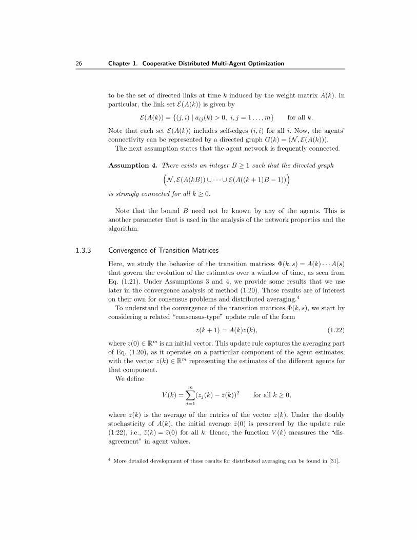
26 Chapter 1. Cooperative Distributed Multi-Agent Optimization
to be the set of directed links at time k induced by the weight matrix A(k). Inparticular, the link set E(A(k)) is given by
E(A(k)) = {(j, i) | aij(k) > 0, i, j = 1 . . . , m} for all k.
Note that each set E(A(k)) includes self-edges (i, i) for all i. Now, the agents’connectivity can be represented by a directed graph G(k) = (N , E(A(k))).
The next assumption states that the agent network is frequently connected.
Assumption 4. There exists an integer B ≥ 1 such that the directed graph(N , E(A(kB)) ∪ · · · ∪ E(A((k + 1)B − 1))
)
is strongly connected for all k ≥ 0.
Note that the bound B need not be known by any of the agents. This isanother parameter that is used in the analysis of the network properties and thealgorithm.
1.3.3 Convergence of Transition Matrices
Here, we study the behavior of the transition matrices Φ(k, s) = A(k) · · ·A(s)that govern the evolution of the estimates over a window of time, as seen fromEq. (1.21). Under Assumptions 3 and 4, we provide some results that we uselater in the convergence analysis of method (1.20). These results are of intereston their own for consensus problems and distributed averaging.4
To understand the convergence of the transition matrices Φ(k, s), we start byconsidering a related “consensus-type” update rule of the form
z(k + 1) = A(k)z(k), (1.22)
where z(0) ∈ Rm is an initial vector. This update rule captures the averaging partof Eq. (1.20), as it operates on a particular component of the agent estimates,with the vector z(k) ∈ Rm representing the estimates of the different agents forthat component.
We define
V (k) =m∑
j=1
(zj(k)− z(k))2 for all k ≥ 0,
where z(k) is the average of the entries of the vector z(k). Under the doublystochasticity of A(k), the initial average z(0) is preserved by the update rule(1.22), i.e., z(k) = z(0) for all k. Hence, the function V (k) measures the “dis-agreement” in agent values.
4 More detailed development of these results for distributed averaging can be found in [31].

Cooperative Distributed Multi-Agent Optimization 27
In the next lemma, we give a bound on the decrease of the agent disagreementV (kB), which is linear in η and quadratic in m−1. This bound plays a crucial rolein establishing the convergence and rate of convergence of transition matrices,which subsequently are used to analyze the method.
Lemma 1.4. Let Assumptions 3 and 4 hold. Then, V (k) is nonincreasing in k.Furthermore,
V ((k + 1)B) ≤(1− η
2m2
)V (kB) for all k ≥ 0.
Proof. This is an immediate consequence of Lemma 5 in [31], stating that5 underAssumptions 3 and 4, for all k with V (kB) > 0,
V (kB)− V ((k + 1)B)V (kB)
≥ η
2m2.
Q.E.D.
Using Lemma 1.4, we establish the convergence of the transition matricesΦ(k, s) of Eq. (1.21) to the matrix with all entries equal to 1
m , and we providea bound on the convergence rate. In particular, we show that the differencebetween the entries of Φ(k, s) and 1
m converges to zero with a geometric rate.
Theorem 1.2. Let Assumptions 3 and 4 hold. Then, for all i, j and all k, s withk ≥ s, we have
∣∣∣∣[Φ(k, s)]ij − 1m
∣∣∣∣ ≤(1− η
4m2
)d k−s+1B e−2
.
Proof. By Lemma 1.4, we have for all k ≥ s,
V (kB) ≤(1− η
2m2
)k−s
V (sB).
Let k and s be arbitrary with k ≥ s, and let
τB ≤ s < (τ + 1)B, tB ≤ k < (t + 1)B,
with τ ≤ t. Hence, by the nonincreasing property of V (k), we have
V (k) ≤ V (tB)
≤(1− η
2m2
)t−τ−1
V ((τ + 1)B)
≤(1− η
2m2
)t−τ−1
V (s).
Note that k − s < (t− τ)B + B implying that k−s+1B ≤ t− τ + 1, where we used
the fact that both sides of the inequality are integers. Therefore dk−s+1B e − 2 ≤
5 The assumptions in [31] are actually weaker.

28 Chapter 1. Cooperative Distributed Multi-Agent Optimization
t− τ − 1, and we have for all k and s with k ≥ s,
V (k) ≤(1− η
2m2
)d k−s+1B e−2
V (s). (1.23)
By Eq. (1.22), we have z(k + 1) = A(k)z(k), and therefore z(k + 1) = Φ(k, s)z(s)for all k ≥ s. Let ei ∈ Rm denote the vector with entries all equal to 0, exceptfor the i-th entry which is equal to 1. Letting z(s) = ei we obtain z(k + 1) =[Φ(k, s)]′i, where [Φ(k, s)]′i denotes the transpose of the i-th row of the matrix.Using the inequalities (1.23) and V (ei) ≤ 1, we obtain
V ([Φ(k, s)]′i) ≤(1− η
2m2
)d k−s+1B e−2
.
The matrix Φ(k, s) is doubly stochastic, because it is the product of doublystochastic matrices. Thus, the average entry of [Φ(k, s)]i is 1/m implying thatfor all i and j,
([Φ(k, s)]ij − 1
m
)2
≤ V ([Φ(k, s)]′i)
≤(1− η
2m2
)d k−s+1B e−2
.
From the preceding relation and√
1− η/(2m2) ≤ 1− η/(4m2), we obtain∣∣∣∣[Φ(k, s)]ij − 1
m
∣∣∣∣ ≤(1− η
4m2
)d k−s+1B e−2
.
Q.E.D.
1.3.4 Convergence Analysis of the Subgradient Method
Here, we study the convergence properties of the subgradient method (1.20) and,in particular, we obtain a bound on the performance of the algorithm. In whatfollows, we assume the uniform boundedness of the set of subgradients of thecost functions fi at all points: for some scalar L > 0, we have for all x ∈ Rn andall i,
‖g‖ ≤ L for all g ∈ ∂fi(x), (1.24)
where ∂fi(x) is the set of all subgradients of fi at x.The analysis combines the proof techniques used for consensus algorithms and
approximate subgradient methods. The consensus analysis rests on the conver-gence rate result of Theorem 1.2 for transition matrices, which provides a tool formeasuring the “agent disagreements” ‖xi(k)− xj(k)‖ in time. Equivalently, wecan measure ‖xi(k)− xj(k)‖ in terms of the disagreements ‖xi(k)− y(k)‖ withrespect to an auxiliary sequence {y(k)}, defined appropriately. The sequence{yk} will also serve as a basis for understanding the effects of subgradient stepsin the algorithm. In fact, we will establish suboptimality property of the sequence

Cooperative Distributed Multi-Agent Optimization 29
{yk}, and then using the estimates for the disagreements ‖xi(k)− y(k)‖, we willprovide a performance bound for the algorithm.
Disagreement EstimateTo estimate the agent “disagreements”, we use an auxiliary sequence {y(k)} ofreference points, defined as follows6:
y(k + 1) = y(k)− α
m
m∑
i=1
di(k), (1.25)
where di(k) is the same subgradient of fi(x) at x = xi(k) that is used in themethod (1.20), and
y(0) =1m
m∑
i=1
xi(0).
In the following lemma, we estimate the norms of the differences xi(k)− y(k) ateach time k. The result relies on Theorem 1.2.
Lemma 1.5. Let Assumptions 3 and 4 hold. Assume also that the subgradientsof each fi are uniformly bounded by some scalar L [cf. Eq. (1.24)]. Then for alli and k ≥ 1,
‖xi(k)− y(k)‖ ≤ βdkB e−2
m∑
j=1
‖xj(0)‖+ αL
(2 +
mB
β(1− β)
),
where β = 1− η4m2 .
Proof. From the definition of the sequence {y(k)} in (1.25) it follows for all k,
y(k) =1m
m∑
i=1
xi(0)− α
m
k−1∑r=0
m∑
i=1
di(r). (1.26)
As given in equation (1.21), for the agent estimates xi(k) we have for all k,
xi(k + 1) =m∑
j=1
[Φ(k, s)]ijxj(s)− α
k−1∑r=s
m∑
j=1
[Φ(k, r + 1)]ijdj(r)− α di(k).
From this relation (with s = 0), we see that for all k ≥ 1,
xi(k) =m∑
j=1
[Φ(k − 1, 0)]ijxj(0)− α
k−2∑r=0
m∑
j=1
[Φ(k − 1, r + 1)]ijdj(r)− α di(k − 1).
(1.27)
6 The iterates y(k) can be associated with a stopped process related to algorithm (1.20), asdiscussed in [40].

30 Chapter 1. Cooperative Distributed Multi-Agent Optimization
By using the relations in Eqs. (1.26) and (1.27), we obtain for all k ≥ 1,
xi(k)− y(k) =m∑
j=1
([Φ(k − 1, 0)]ij − 1
m
)xj(0)
− α
k−2∑r=0
m∑
j=1
([Φ(k − 1, r + 1)]ij − 1
m
)dj(r)
− α di(k − 1) +α
m
m∑
i=1
di(k − 1).
Using the subgradient boundedness, we obtain for all k ≥ 1,
‖xi(k)− y(k)‖ ≤m∑
j=1
∣∣∣∣[Φ(k − 1, 0)]ij − 1m
∣∣∣∣ ‖xj(0)‖
+αL
k−1∑s=1
m∑
j=1
∣∣∣∣[Φ(k − 1, s)]ij − 1m
∣∣∣∣ + 2αL.
By using Theorem 1.2, we can bound the terms∣∣[Φ(k − 1, s)]ij − 1
m
∣∣ and obtainfor all i and any k ≥ 1,
‖xi(k)− y(k)‖ ≤m∑
j=1
βdkB e−2‖xj(0)‖+ αL
k−1∑s=1
m∑
j=1
βdk−sB e−2 + 2αL
= βdkB e−2
m∑
j=1
‖xj(0)‖+ αLm
k−1∑s=1
βdk−sB e−2 + 2αL.
By using∑k−1
s=1 βdk−sB e−2 ≤ ∑∞
r=1 βdrB e−2 = 1
β
∑∞r=1 βd
rB e−1, and
∞∑r=1
βdrB e−1 =
∞∑r=1
βdrB e−1 ≤ B
∞∑t=0
βt =B
1− β,
we obtaink−1∑s=1
βdk−sB e−2 ≤ B
β(1− β).
Therefore, it follows that for all k ≥ 1,
‖xi(k)− y(k)‖ ≤ βdkB e−2
m∑
j=1
‖xj(0)‖+ αL
(2 +
mB
β(1− β)
).
Q.E.D.

Cooperative Distributed Multi-Agent Optimization 31
Estimate for the Auxiliary SequenceWe next establish a result that estimates the objective function f =
∑mi=1 fi at
the running averages of the vectors y(k) of Eq. (1.25). Specifically, we define
y(k) =1k
k∑
h=1
y(h) for all k ≥ 1,
and we estimate the function values f(y(k)). We have the following result.
Lemma 1.6. Let Assumptions 3 and 4 hold, and assume that the subgradientsare uniformly bounded as in Eq. (1.24). Also, assume that the set X∗ of optimalsolutions of problem (1.19) is nonempty. Then, the average vectors y(k) satisfyfor all k ≥ 1,
f(y(k)) ≤ f ∗ +αL2C
2+
2mLB
kβ(1− β)
m∑
j=1
‖xj(0)‖+m
2αk(dist(y(0), X∗) + αL)2,
where y(0) = 1m
∑mj=1 xj(0), β = 1− η
4m2 and
C = 1 + 4m
(2 +
mB
β(1− β)
).
Proof. From the definition of the sequence y(k) it follows for any x∗ ∈ X∗ andall k,
‖y(k + 1)− x∗‖2 = ‖y(k)− x∗‖2 +α2
m2
∥∥∥∥∥m∑
i=1
dj(k)
∥∥∥∥∥
2
− 2α
m
m∑
i=1
di(k)′(y(k)− x∗).
(1.28)We next estimate the terms di(k)′(y(k)− x∗) where di(k) is a subgradient of fi
at xi(k). For any i and k, we have
di(k)′(y(k)− x∗) = di(k)′(y(k)− xi(k)) + di(k)′(xi(k)− x∗).
By the subgradient property in (1.2), we have di(k)(xi(k)− x∗) ≥ fi(xi(k))−fi(x∗) implying
di(k)′(y(k)− x∗) ≥ di(k)′(y(k)− xi(k)) + fi(xi(k))− fi(x∗)≥ −L‖y(k)− xi(k)‖+ [fi(xi(k))− fi(y(k))] + [fi(y(k))− fi(x∗)],
where the last inequality follows from the subgradient boundedness. We nextconsider fi(xi(k))− fi(y(k)), for which by subgradient property (1.2) we have
fi(xi(k))− fi(y(k)) ≥ di(k)′(xi(k)− y(k)) ≥ −L‖xi(k)− y(k)‖,where di(k) is a subgradient of fi at y(k), and the last inequality follows fromthe subgradient boundedness. Thus, by combining the preceding two relations,we have for all i and k,
di(k)′(y(k)− x∗) ≥ −2L‖y(k)− xi(k)‖+ fi(y(k))− fi(x∗).

32 Chapter 1. Cooperative Distributed Multi-Agent Optimization
By substituting the preceding estimate for di(k)′(y(k)− x∗) in relation (1.28),we obtain
‖y(k + 1)− x∗‖2 ≤ ‖y(k)− x∗‖2 +α2
m2
∥∥∥∥∥m∑
i=1
dj(k)
∥∥∥∥∥
2
+4Lα
m
m∑
i=1
‖y(k)− xi(k)‖
−2α
m
m∑
i=1
fi(y(k))− fi(x∗).
By using the subgradient boundedness and noting that f =∑m
i=1 fi and f(x∗) =f ∗, we can write
‖y(k + 1)− x∗‖2 ≤ ‖y(k)− x∗‖2 +α2L2
m+
4αL
m
m∑
i=1
‖y(k)− xi(k)‖
−2α
m(f(y(k))− f ∗) .
Taking the minimum over x∗ ∈ X∗ in both sides of the preceding relation, weobtain
dist2(y(k + 1), X∗) ≤ dist2(y(k), X∗) +α2L2
m+
4αL
m
m∑
i=1
‖y(k)− xi(k)‖
−2α
m(f(y(k))− f ∗) .
Using Lemma 1.5 to bound each of the terms ‖y(k)− xi(k)‖, we further obtain
dist2(y(k + 1), X∗) ≤ dist2(y(k), X∗) +α2L2
m+ 4αLβd k
B e−2m∑
j=1
‖xj(0)‖
+4α2L2
(2 +
mB
β(1− β)
)− 2α
m[f(y(k))− f ∗] .
Therefore, by regrouping the terms and introducing
C = 1 + 4m
(2 +
mB
β(1− β)
),
we have for all k ≥ 1,
f(y(k)) ≤ f ∗ +αL2C
2+ 2mLβd k
B e−2m∑
j=1
‖xj(0)‖
+m
2α
(dist2(y(k), X∗)− dist2(y(k + 1), X∗)
).
By adding these inequalities for different values of k, we obtain
1k
k∑
h=1
f(y(h)) ≤ f ∗ +αL2C
2+
2mLB
kβ(1− β)
m∑
j=1
‖xj(0)‖
+m
2αk
(dist2(y(1), X∗)− dist2(y(k), X∗)
), (1.29)

Cooperative Distributed Multi-Agent Optimization 33
where we use the following inequality for t ≥ 1,
t∑
k=1
βd kB e−2 ≤ 1
β
∞∑
k=1
βd kB e−1 ≤ B
β
∞∑s=1
βs =B
β(1− β).
By discarding the nonpositive term on the right hand side in relation (1.29) andby using the convexity of f ,
1k
k∑
h=1
f(y(h)) ≤ f ∗ +αL2C
2+
2mLB
kβ(1− β)
m∑
j=1
‖xj(0)‖
+m
2αkdist2(y(1), X∗).
Finally, by using the definition of y(k) in (1.25) and the subgradient boundedness,we see that
dist2(y(1), X∗) ≤ (dist(y(0), X∗) + αL)2 ,
which when combined with the preceding relation yields the desired inequality.Q.E.D.
Performance Bound for the AlgorithmWe establish a bound on the performance of the algorithm at the time-averageof the vectors xi(k) generated by method (1.20). In particular, we define thevectors xi(k) as follows:
xi(k) =1k
k∑
h=1
xi(h).
The use of these vectors allows us to bound the objective function improvementat every iteration, by combining the estimates for ‖xi(k)− y(k)‖ of Lemma 1.5and the estimates for f(y(k)) of Lemma 1.6. We have the following.
Theorem 1.3. Let Assumptions 3 and 4 hold, and assume that the set X∗ ofoptimal solutions of problem (1.19) is nonempty. Let the subgradients be boundedas in Eq. (1.24). Then, the averages xi(k) of the iterates obtained by the method(1.20) satisfy for all i and k ≥ 1,
f(xi(k)) ≤ f ∗ +αL2C1
2+
4mLB
kβ(1− β)
m∑
j=1
‖xj(0)‖+m
2αk(dist(y(0), X∗) + αL)2,
where y(0) = 1m
∑mj=1 xj(0), β = 1− η
4m2 and
C1 = 1 + 8m
(2 +
mB
β(1− β)
).

34 Chapter 1. Cooperative Distributed Multi-Agent Optimization
Proof. By the convexity of the functions fj , we have, for any i and k ≥ 1,
f(xi(k)) ≤ f(y(k)) +m∑
j=1
gij(k)′(xi(k)− y(k)),
where gij(k) is a subgradient of fj at xi(k). Then, by using the subgradientboundedness, we obtain for all i and k ≥ 1,
f(xi(k)) ≤ f(y(k)) +2L
k
m∑
i=1
(k∑
t=1
‖xi(t)− y(t)‖)
. (1.30)
By using the bound for ‖xi(k)− y(k)‖ of Lemma 1.5, we have for all i and k ≥ 1,
k∑t=1
‖xi(t)− y(t)‖ ≤(
k∑t=1
βd tB e−2
)m∑
j=1
‖xj(0)‖+ αkL
(2 +
mB
β(1− β)
).
Noting that
k∑t=1
βd tB e−2 ≤ 1
β
∞∑t=1
βd tB e−1 ≤ B
β
∞∑s=1
βs =B
β(1− β),
we obtain for all i and k ≥ 1,
k∑t=1
‖xi(t)− y(t)‖ ≤ B
β(1− β)
m∑
j=1
‖xj(0)‖+ αkL
(2 +
mB
β(1− β)
).
Hence, by summing these inequalities over all i and by substituting the resultingestimate in relation (1.30), we obtain
f(xi(k)) ≤ f(y(k)) +2mLB
kβ(1− β)
m∑
j=1
‖xj(0)‖+ 2mαL2
(2 +
mB
β(1− β)
).
The result follows by using the estimate for f(y(k)) of Lemma 1.6. Q.E.D.
The result of Theorem 1.3 provides an estimate on the values f(xi(k)) periteration k. As the number of iterations increases to infinity the last two termsof the estimate diminish, resulting with
lim supk→∞
f(xi(k)) ≤ f ∗ +αL2C1
2for all i.
As seen from Theorem 1.3, the constant C1 increases only polynomially withm. When α is fixed and the parameter η is independent of m, the largest erroris of the order of m4, indicating that for high accuracy, the stepsize needs tobe very small. However, our bound is for general convex functions and networktopologies, and further improvements of the bound are possible for special classesof convex functions and special topologies.

Cooperative Distributed Multi-Agent Optimization 35
1.4 Extensions
Here, we consider extensions of the distributed model of Section 1.3 to account forvarious network effects. We focus on two such extensions. The first is an extensionof the optimization model (1.20) to a scenario where the agents communicateover a network with finite bandwidth communication links, and the second is anextension of the consensus problem to the scenario where each agent is facingsome constraints on its decisions. We discuss these extensions in the followingsections.
1.4.1 Quantization Effects on Optimization
Here, we discuss the agent system where the agents communicate over a net-work consisting of finite bandwidth links. Thus, the agents cannot exchangecontinuous-valued information (real numbers), but instead can only send quan-tized information. This problem has recently gained interest in the networkingliterature [22, 12, 13, 31]. In what follows, we present recent results dealing withthe effects of quantization on the multi-agent distributed optimization over a net-work. More specifically, we discuss a “quantized” extension of the subgradientmethod (1.20) and provide a performance bound.7
We consider the case where the agents exchange quantized data, but they canstore continuous data. In particular, we assume that each agent receives andsends only quantized estimates, i.e., vectors whose entries are integer multiplesof 1/Q, where Q is some positive integer. At time k, an agent receives quan-tized estimates xQ
j (k) from some of its neighbors and updates according to thefollowing rule:
xQi (k + 1) =
m∑
j=1
aij(k)xQj (k)− αdi(k)
, (1.31)
where di(k) is a subgradient of fi at xQi (k), and byc denotes the operation of
(componentwise) rounding the entries of a vector y to the nearest multiple of1/Q. We also assume that the agents’ initial estimates xQ
j (0) are quantized.We can view the agent estimates in Eq. (1.31) as consisting of a consensus part∑mj=1 aij(k)xQ
j (k), and the term due to the subgradient step and an error (dueto extracting the consensus part). Specifically, we rewrite Eq. (1.31) as follows:
xQi (k + 1) =
m∑
j=1
aij(k)xQj (k)− αdi(k)− εi(k + 1), (1.32)
7 The result presented here can be found with more details in [32].
36 Chapter 1. Cooperative Distributed Multi-Agent Optimization
where the error vector εi(k + 1) is given by
εi(k + 1) =m∑
j=1
aij(k)xQj (k)− αdi(k)− xQ
i (k + 1).
Thus, the method can be viewed as a subgradient method using consensus andwith external (possibly persistent) noise, represented by εi(k + 1). Due to therounding down to the nearest multiple of 1/Q, the error vector εi(k + 1) satisfies
0 ≤ εi(k + 1) ≤ 1Q
1 for all i and k,
where the inequalities above hold componentwise and 1 denotes the vector inRn with all entries equal to 1. Therefore, the error norms ‖εi(k)‖ are uniformlybounded in time and across agents. In fact, it turns out that these errors convergeto 0 as k increases. These observations are guiding the analysis of the algorithm.
Performance Bound for the Quantized MethodWe next give a performance bound for the method (1.31) assuming that theagents can store perfect information (infinitely many bits). We consider the time-average of the iterates xQ
i (k), defined by
xQi (k) =
1k
k∑
h=1
xQi (h) for k ≥ 1.
We have the following result (see [32] for the proof).
Theorem 1.4. Let Assumptions 3 and 4 hold, and assume that the optimal setX∗ of problem (1.19) is nonempty. Let subgradients be bounded as in Eq. (1.24).Then, for the averages xQ
i (k) of the iterates obtained by the method (1.31) satisfyfor all i and all k ≥ 1,
f(xQi (k)) ≤ f ∗ +
αL2C1
2+
4mLB
kβ(1− β)
m∑
j=1
‖xQj (0)‖
+m
2αk
(dist(y(0), X∗) + αL +
√n
Q
)2
,
where y(0) = 1m
∑mj=1 xQ
j (0), β = 1− η4m2 and
C1 = 1 + 8m
(1 +
√n
αLQ
)(2 +
mB
β(1− β)
).
Theorem 1.4 provides an estimate on the values f(xQi (k)) per iteration k. As
the number of iterations increases to infinity the last two terms of the estimatevanish, yielding
lim supk→∞
f(xQi (k)) ≤ f ∗ +
αL2C1
2for all i,

Cooperative Distributed Multi-Agent Optimization 37
with
C1 = 1 + 8m
(1 +
√n
αLQ
)(2 +
mB
β(1− β)
).
The constant C1 increases only polynomially with m. In fact, the growth withm is the same as that of the bound given in Theorem 1.3, since the result inTheorem 1.3 follows from Theorem 1.4. In particular, by letting the quantizationlevel Q be increasingly finer (i.e., Q →∞), we see that the constant C1 satisfies
limQ→∞
C1 = 1 + 8m
(2 +
mB
β(1− β)
),
which is the same as the constant C1 in Theorem 1.3. Hence, in the limit asQ →∞, the estimate in Theorem 1.4 yields the estimate in Theorem 1.3.
1.4.2 Consensus with Local Constraints
Here, we focus only on the problem of reaching a consensus when the estimatesof different agents are constrained to lie in different constraint sets and eachagent only knows its own constraint set. Such constraints are significant in anumber of applications including signal processing within a network of sensors,network motion planning and alignment, rendezvous problems and distributedconstrained multi-agent optimization problems8, where each agent’s position islimited to a certain region or range.
As in the preceding, we denote by xi(k) the estimate generated and storedby agent i at time slot k. The agent estimate xi(k) ∈ Rn is constrained to liein a nonempty closed convex set Xi ⊆ Rn known only to agent i. The agents’objective is to cooperatively reach a consensus on a common vector through asequence of local estimate updates (subject to the local constraint set) and localinformation exchanges (with neighboring agents only).
To generate the estimate at time k + 1, agent i forms a convex combination ofits estimate xi(k) with the estimates received from other agents at time k, andtakes the projection of this vector on its constraint set Xi. More specifically, agenti at time k + 1 generates its new estimate according to the following relation:
xi(k + 1) = PXi
m∑
j=1
aij(k)xj(k)
. (1.33)
Through the rest of the discussion, the constraint sets X1, . . . , Xm are assumedto be closed convex subsets of Rn.
The relation in (1.33) defines the projected consensus algorithm . The methodcan be viewed as a distributed algorithm for finding a point in common to theclosed convex sets X1, . . . , Xm. This problem can be formulated as an uncon-
8 See also [28] for constrained consensus arising in connection with potential games.

38 Chapter 1. Cooperative Distributed Multi-Agent Optimization
strained convex minimization, as follows
minimize 12
∑mi=1 ‖x− PXi
[x]‖2subject to x ∈ Rn.
(1.34)
In view of this optimization problem, the method in (1.33) can be interpreted asa distributed algorithm where an agent i is assigned an objective function fi(x) =12 ‖x− PXi
[x]‖2. Each agent updates its estimate by taking a step (with step-length equal to 1) along the negative gradient of its own objective function fi =12 ‖x− PXi
‖2 at x =∑m
j=1 aij(k)xj(k). This interpretation of the update rulemotivates our line of analysis of the projected consensus method. In particular,we use
∑mi=1 ‖xi(k)− x‖2 with x ∈ ∩m
i=1Xi as a function measuring the progressof the algorithm.
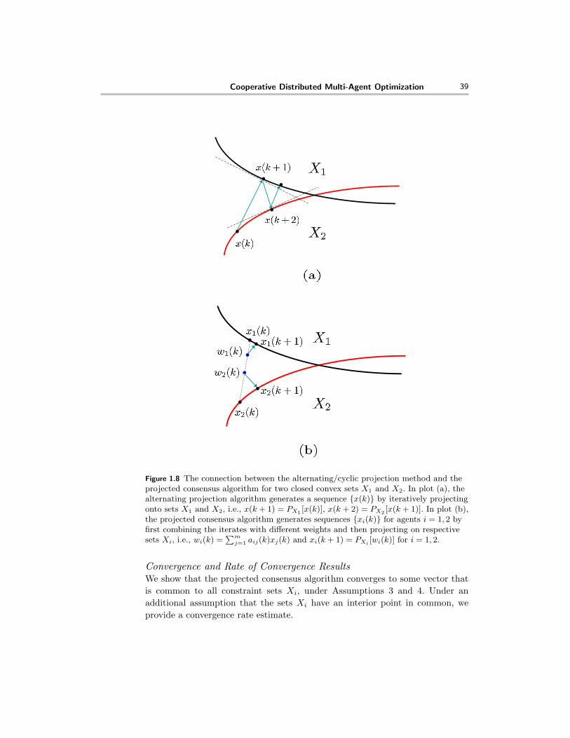
Let us note that the method of Eq. (1.33), with the right choice of the weightsaij(k), corresponds to the classical alternating or cyclic projection method. Thesemethods generate a sequence of vectors by projecting iteratively on the sets(either cyclically or with some given order), see Figure 1.8(a) . The convergencebehavior of these methods has been established by Von Neumann [43] and Aron-szajn [1], Gubin et al. [17], Deutsch [15], and Deutsch and Hundal [16]. Theprojected consensus algorithm can be viewed as a version of the alternating pro-jection algorithm, where the iterates are combined with the weights varying overtime and across agents, and then projected on the individual constraint sets.
To study the convergence behavior of the agent estimates {xi(k)} defined inEq. (1.33), we find it useful to decompose the representation of the estimates in alinear part (corresponding to nonprojected consensus) and a nonlinear part (cor-responding to the difference between the projected and nonprojected consensus).Specifically, we re-write the update rule in (1.33) as
xi(k + 1) =m∑
j=1
aij(k)xj(k) + ei(k), (1.35)
where ei(k) represents the error due to the projection operation, given by
ei(k) = PXi
m∑
j=1
aij(k)xj(k)
−
m∑
j=1
aij(k)xj(k). (1.36)
As indicated by the preceding two relations, the evolution dynamics of the esti-mates xi(k) for each agent is decomposed into a sum of a linear (time-varying)term
∑mj=1 aij(k)xj(k) and a nonlinear term ei(k). The linear term captures the
effects of mixing the agent estimates, while the nonlinear term captures the non-linear effects of the projection operation. This decomposition can be exploitedto analyze the behavior and estimate the performance of the algorithm. It canbe seen [41] that, under the doubly stochasticity assumption on the weights,the nonlinear terms ei(k) are diminishing in time for each i, and therefore, theevolution of agent estimates is “almost linear”. Thus, the nonlinear term can beviewed as a non-persistent disturbance in the linear evolution of the estimates.
Cooperative Distributed Multi-Agent Optimization 39
Figure 1.8 The connection between the alternating/cyclic projection method and theprojected consensus algorithm for two closed convex sets X1 and X2. In plot (a), thealternating projection algorithm generates a sequence {x(k)} by iteratively projectingonto sets X1 and X2, i.e., x(k + 1) = PX1 [x(k)], x(k + 2) = PX2 [x(k + 1)]. In plot (b),the projected consensus algorithm generates sequences {xi(k)} for agents i = 1, 2 byfirst combining the iterates with different weights and then projecting on respectivesets Xi, i.e., wi(k) =
∑mj=1 aij(k)xj(k) and xi(k + 1) = PXi
[wi(k)] for i = 1, 2.
Convergence and Rate of Convergence ResultsWe show that the projected consensus algorithm converges to some vector thatis common to all constraint sets Xi, under Assumptions 3 and 4. Under anadditional assumption that the sets Xi have an interior point in common, weprovide a convergence rate estimate.

40 Chapter 1. Cooperative Distributed Multi-Agent Optimization
The following result shows that the agents reach a consensus asymptotically,i.e., the agent estimates xi(k) converge to the same point as k goes to infinity(see [41]).
Theorem 1.5. Let the constraint sets X1, . . . , Xm be closed convex subsets ofRn, and let the set X = ∩m
i=1Xi be nonempty. Also, let Assumptions 3 and 4 hold.Let the sequences {xi(k)}, i = 1 . . . , m, be generated by the projected consensusalgorithm (1.33). We then have for some x ∈ X,
limk→∞
‖xi(k)− x‖ = 0 for all i.
We next provide a rate estimate for the projected consensus algorithm (1.33).It is difficult to access the convergence rate in the absence of any specific structureon the constraint sets Xi. To deal with this, we consider a special case when theweights are time-invariant and equal, i.e., aij(k) = 1/m for all i, j and k, and theintersection of the sets Xi has a nonempty interior. In particular, we have thefollowing rate result (see [41]).
Theorem 1.6. Let the constraint sets X1, . . . , Xm be closed convex subsets ofRn. Let X = ∩m
i=1Xi, and assume that there is a vector x ∈ X and a scalar δ > 0such that
{z | ‖z − x‖ ≤ δ} ⊂ X.
Also, let Assumption 4 hold. Let the sequences {xi(k)}, i = 1 . . . , m be generatedby the algorithm (1.33), where the weights are uniform, i.e., aij(k) = 1/m forall i, j and k. We then have
m∑
i=1
‖xi(k)− x‖2 ≤(
1− 14R2
)k m∑
i=1
‖xi(0)− x‖2 for all k ≥ 0,
where x ∈ X is the common limit of the sequences {xi(k)}, i = 1 . . . , m, andR = 1
δ
∑mi=1 ‖xi(0)− x‖.
The result shows that the projected consensus algorithm converges with ageometric rate under the interior point and uniform weights assumptions.
1.5 Future Work
The models presented so far highlight a number of fruitful areas for futureresearch. These include but are not limited to the following topics.

Cooperative Distributed Multi-Agent Optimization 41
1.5.1 Optimization with Delays
The distributed subgradient algorithm we presented in Section 1.3 [cf. Eq. (1.20)]assumes that at any time k ≥ 0, agent i has access to estimates xj(k) of itsneighbors. This may not be possible in communication networks where there aredelays associated with transmission of agent estimates over a communicationchannel. A natural extension therefore is to study an asynchronous operation ofthe algorithm (1.20) using delayed agent values, i.e., agent i at time k has accessto outdated values of agent j.
More formally, we consider the following update rule for agent i: Suppose agentj sends its estimate xj(s) to agent i. If agent i receives the estimate xj(s) attime k, then the delay is tij(k) = k − s and agent i assigns a weight aij(k) > 0to the estimate xj(s). Otherwise, agent i uses aij(k) = 0. Hence, each agent i
updates its estimate according to the following relation:
xi(k + 1) =m∑
j=1
aij(k)xj(k − tij(k))− αdi(k) for k = 0, 1, 2, . . . , (1.37)
where the vector xi(0) ∈ Rn is the initial estimate of agent i, the scalar tij(k)is nonnegative and it represents the delay of a message from agent j to agent i,while the scalar aij(k) is a nonnegative weight that agent i assigns to a delayedestimate xj(s) arriving from agent j at time k.
Establishing the convergence and rate properties of the update rule (1.37)is essential in understanding the robustness of the optimization algorithm todelays and dynamics associated with information exchange over finite bandwidthcommunication channels. Under the assumption that all delay values are bounded[i.e., there exists a scalar B > 0 such that tij(k) ≤ B for all i, j ∈ N and all k ≥0], the update rule (1.37) can be analyzed by considering an augmented model,where we introduce “artificial” agents for handling the delayed information only.In particular, with each agent i of the original model, we associate a new agentfor each of the possible values of the delay that a message originating from agenti may experience. In view of the bounded delay values assumption, it suffices toadd finitely many new agents handling the delays. This augmentation reducesthe delayed multi-agent model into a model without delays (see Figure 1.5.1).
The augmented agent model is used in [35] to study the consensus problem inthe presence of delays. In particular, this paper shows that agents reach consensuson a common decision even with delayed information and establishes convergencerate results. Future work includes analyzing the optimization algorithm of (1.20)in the presence of delays. The analysis of the optimization algorithm is morechallenging in view of the fact that due to delays, an agent may receive differentamount of information from different agents. This difference in the update fre-quencies results in the overall consensus value to be influenced more by some ofthe agents’ information (about their local objective function). Thus, the valuethat agents reach a consensus on need not be the optimal solution of the problemof minimizing the sum of the local objective functions of the agents. To address

42 Chapter 1. Cooperative Distributed Multi-Agent Optimization
(a)
(b)
Figure 1.9 Plot (a) illustrates an agent network with 3 agents, where agents 1 and 2,and agents 2 and 3 communicate directly. Plot (b) illustrates the augmented networkassociated with the original network of part (a), when the delay value between agentsis bounded by 3. The artificial agents introduced in the system are 4, . . . , 9. Agents 4,5, and 6 model the delay of 1 while agents 7, 8, and 9 model the delay of 2 for theoriginal nodes 1, 2 and 3, respectively.
this issue, the optimization algorithm should be modified to include the updatefrequency information in the agent exchange model.
1.5.2 Optimization with Constraints
Section 1.3 presents a distributed subgradient method for solving the uncon-strained optimization problem (1.19). An important extension is to develop opti-mization methods for solving multi-agent optimization problems in which eachagent i has a local convex closed constraint set Xi ⊆ Rn know by agent i only.Note that the case when there is a global constraint Cg ⊆ Rn is a special case ofthis problem with Xi = Cg for all i ∈ N (see Introduction).
An immediate solution for this problem is to combine the subgradient algo-rithm (1.20) with the projected consensus algorithm studied in Section 1.4.2.More specifically, we denote by xi(k) the estimate maintained by agent i at timeslot k. Agent i updates this estimate by forming a convex combination of thisestimate with the estimates received from his neighbors at time k, taking a step(with stepsize α) in the direction of the subgradient of his local convex objectivefunction fi at xi(k), and taking the projection of this vector on its constraint setXi, i.e., agent i at time k generates its new estimate according to
xi(k + 1) = PXi
m∑
j=1
aij(k)xj(k)− αdi(k)
for k = 0, 1, 2, . . . . (1.38)

Cooperative Distributed Multi-Agent Optimization 43
The convergence analysis of this algorithm involves combining the ideas andmethods of Sections 1.3 and 1.4.2, i.e., understanding the behavior of the tran-sition matrices, the approximate subgradient method, and the projection errors.It is more challenging due to the dependencies of the error terms involved in theanalysis.
When the global constraint set Cg has more structure, e.g., when it can beexpressed as finitely many equality and inequality constraints, it may be possibleto develop primal-dual algorithms, which combine the primal step (1.20) with adual step for updating the dual solutions (or multipliers), as in Section 1.2.Primal-dual subgradient methods have been analyzed in recent work [38] for amodel in which each agent has the same information set, i.e., at each time slot,each agent has access to the same estimate. It would be of great interest tocombine this model with the multi-agent model of Section 1.3 that incorporatesdifferent local information structures.
1.5.3 Nonconvex Local Objective Functions
The distributed optimization framework presented in Section 1.3 is very generalin that it encompasses local information structures, operates with time-varyingconnectivity, and optimizes general convex local objective functions subject toconvex constraints. However, there are many applications such as inelastic ratecontrol for voice communication (see [49, 18]) and rendezvous problems with con-straints (see [28]) in which the local objective functions and constraints are notconvex. Under smoothness assumptions on the objective functions, the methodspresented in this chapter can still be used and guarantee convergence to station-ary points. An important future direction is the design of algorithms that canguarantee convergence to global optimal in the presence of nonconvexities andin decentralized environments.
1.6 Conclusions
This chapter presents a general framework for distributed optimization of amulti-agent networked system. In particular, we consider multiple agents, eachwith its own private local objective function and local constraint, which exchangeinformation over a network with time-varying connectivity. The goal is to designalgorithms that the agents can use to cooperatively optimize a global objectivefunction, which is a function of the local objective functions, subject to localand global constraints. A key characteristic of these algorithms is their oper-ation within the informational constraints of the model, specified by the localinformation structures and the underlying connectivity of the agents.
Our development focuses on two key approaches. The first approach usesLagrangian duality and dual subgradient methods to design algorithms. Thesealgorithms yield distributed methods for problems with separable structure (i.e.,

44 Chapter 1. Cooperative Distributed Multi-Agent Optimization
problems where local objective functions and constraints decompose over thecomponents of the decision vector), as illustrated in Section 1.2.3. Since thesemethods operate in the dual space, a particular interest is in producing primalnear-feasible and near-optimal solutions using the information generated by thedual subgradient algorithm. The analysis presented in Section 1.2 is from ourrecent work [34, 39], which discusses approximate primal solution recovery andprovides convergence rate estimates on the generated solutions.
The second approach combines subgradient methods with consensus algo-rithms to optimize general convex local objective functions in decentralized set-tings. Even though the nonseparable structure of the local objective functionsdoes not immediately lead to decomposition schemes, the consensus part includedin the algorithm serves as a mechanism to distribute the computations amongthe agents. The material presented in Sections 1.3 and 1.4 combines results froma series of recent papers (see [40, 33, 35, 41, 31, 32]).
This chapter illustrates the challenges associated with optimization algorithmdesign for multi-agent networked systems. Optimization methodologies haveplayed a key role in providing a systematic framework for the design of archi-tectures and new protocols in many different networks. For such applications,it is clear that many of the assumptions we take for granted in the develop-ment and analysis of algorithms for solving constrained optimization problemsare not valid. These include assumptions such as global access to input data andability to exchange real-valued variables instantly between different processors.Moreover, practical considerations divert our attention from complicated stepsizerules that can guarantee convergence to an optimal solution to simple stepsizerules (such as a constant stepsize rule), which may not guarantee convergence,but nevertheless can provide an “approximate solution” within reasonable timeconstraints. The importance of optimization methods for such practical applica-tions motivate development of new frameworks and methods that can operatewithin the constraints imposed by the underlying networked system.
1.7 Problems
Exercise 1. Let {µk} be a dual sequence generated by the subgradient methodwith a constant stepsize α [cf. Eq. (1.8)]. Assume that the subgradients {gk} areuniformly bounded, i.e., ‖gk‖ ≤ L for all k. Assume also that the dual optimalsolution set M ∗ is nonempty.
At each iteration k, consider an approximate dual solution generated by aver-aging the vectors µ0, . . . , µk−1, i.e.,
µk =1k
k−1∑
i=0
µi for all k ≥ 1.

Cooperative Distributed Multi-Agent Optimization 45
Show that
q(µk) ≥ q∗ − dist2(µ0,M∗)
2αk− αL2
2for all k ≥ 1.
Exercise 2. (Minimum Cost Network Flow Problem)Consider a directed connected graph G = (N , E), where N is the node set and
E is the edge set. At each node i, there is a given external source flow bi thatenters (if bi > 0) or leaves (if bi < 0) node i. Let b be the vector b = [bi]i∈N . Wedefine the node-edge incidence matrix A as the |N | × |E| matrix given as follows:the (i, j)th entry [A]ij is given by +1 if edge j leaves node i; by −1 if edge j entersnode i; and 0 otherwise.
Each edge has a convex cost function fi(xi), where xi denotes the flow on edgei. We are interested in finding a flow vector x = [xi]i∈E that minimizes the sumof the edge cost functions. This problem can be formulated as an optimizationproblem as follows:
minimize∑
i∈Efi(xi) (1.39)
subject to Ax = b
x ≥ 0,
where the constraint Ax = b captures the conservation of flow constraints.Use Lagrangian decomposition and the dual subgradient algorithm to solve this
problem. Show that this approach leads to a distributed optimization method forsolving problem (1.39).
Exercises 3–5 are the steps involved in proving the result of Theorem 1.4.
Exercise 3. Consider the quantized method given in (1.31) of Section 1.4.1.Define the transition matrices Φ(k, s) from time s to time k, as follows
Φ(k, s) = A(k)A(k − 1) · · ·A(s) for all s and k with k ≥ s,
(see Section 1.3.1).
(a) Using the transition matrices and the decomposition of the estimate evolu-tion of Eqs. (1.35)–(1.36), show that the relation between xi(k + 1) and theestimates x1(0), . . . , xm(0) is given by
xQi (k + 1) =
m∑
j=1
[Φ(k, 0)]ijxQj (0)− α
k∑s=1
m∑
j=1
[Φ(k, s)]ij dj(s− 1)
−k∑
s=1
m∑
j=1
[Φ(k, s)]ijεj(s)− αdi(k)− εi(k + 1).

46 Chapter 1. Cooperative Distributed Multi-Agent Optimization
(b) Consider an auxiliary sequence {y(k)} defined by
y(k) =1m
m∑
j=1
xQi (k).
Show that for all k,
y(k) =1m
m∑
j=1
xQj (0)− α
m
k∑s=1
m∑
j=1
dj(s− 1)− 1m
k∑s=1
m∑
j=1
εj(s).
(c) Suppose that Assumptions 3 and 4 hold. Using the relations in parts (a) and(b), and Theorem 1.2, show that
‖xQi (k)− y(k)‖ ≤ βd
kB e−2
m∑
j=1
‖xQj (0)‖+
(αL +
√n
Q
)(2 +
mB
β(1− β)
).
Exercise 4. Let y(k) be a sequence defined in Exercise 3. Consider the runningaverages y(k) of the vectors y(k), given by
y(k) =1k
k∑
h=1
y(h) for all k ≥ 1.
Let Assumptions 3 and 4 hold, and assume that the set X∗ of optimal solutionsof problem (1.19) is nonempty. Also, assume that the subgradients are uniformlybounded as in Eq. (1.24). Then, the average vectors y(k) satisfy for all k ≥ 1,
f(y(k)) ≤ f ∗ +αL2C
2+
2mLB
kβ(1− β)
m∑
j=1
‖xQj (0)‖
+m
2αk
(dist(y(0), X∗) + αL +
√n
Q
)2
,
where y(0) = 1m
∑mj=1 xQ
j (0), β = 1− η4m2 , and
C = 1 + 4m
(1 +
√n
αLQ
)(2 +
mB
β(1− β)
).
Exercise 5. Prove Theorem 1.4 using the results of Exercises 3 and 4.
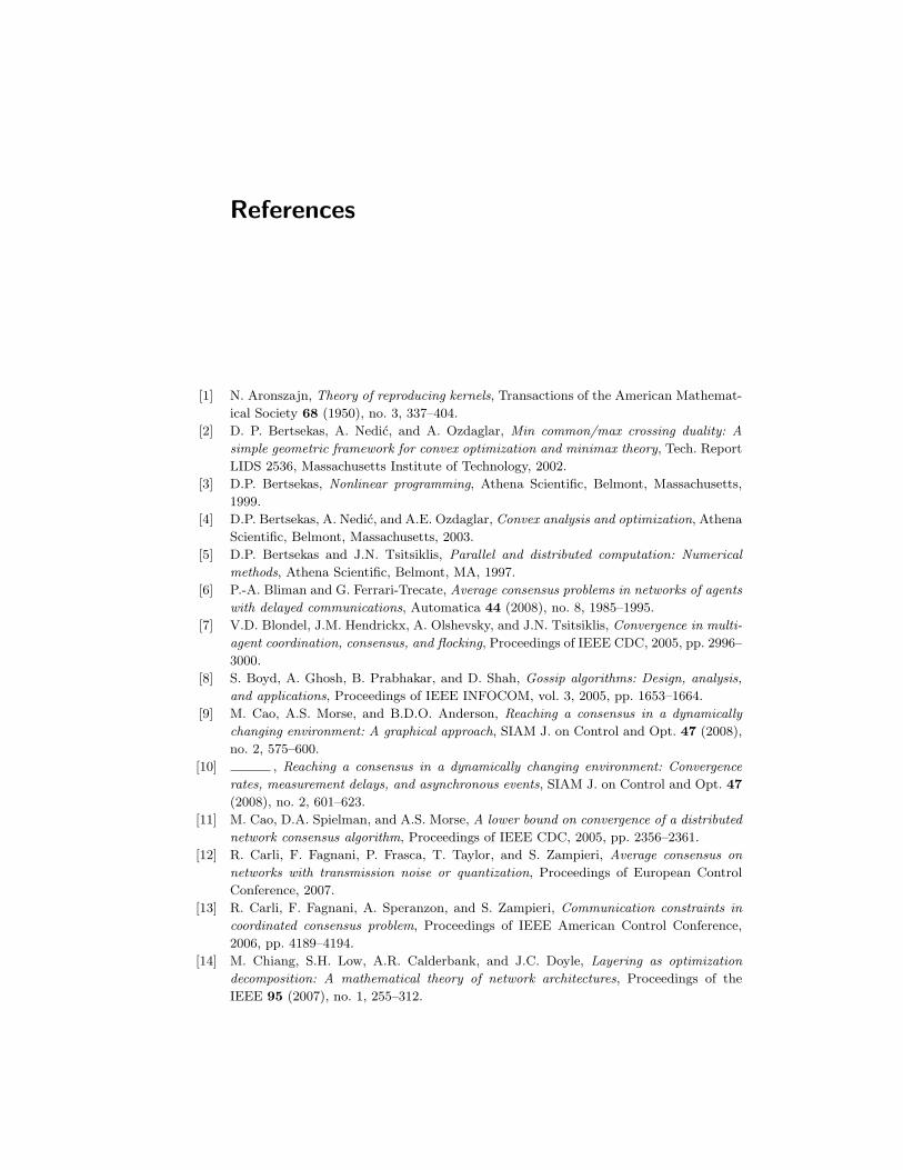
References
[1] N. Aronszajn, Theory of reproducing kernels, Transactions of the American Mathemat-
ical Society 68 (1950), no. 3, 337–404.
[2] D. P. Bertsekas, A. Nedic, and A. Ozdaglar, Min common/max crossing duality: A
simple geometric framework for convex optimization and minimax theory, Tech. Report
LIDS 2536, Massachusetts Institute of Technology, 2002.
[3] D.P. Bertsekas, Nonlinear programming, Athena Scientific, Belmont, Massachusetts,
1999.
[4] D.P. Bertsekas, A. Nedic, and A.E. Ozdaglar, Convex analysis and optimization, Athena
Scientific, Belmont, Massachusetts, 2003.
[5] D.P. Bertsekas and J.N. Tsitsiklis, Parallel and distributed computation: Numerical
methods, Athena Scientific, Belmont, MA, 1997.
[6] P.-A. Bliman and G. Ferrari-Trecate, Average consensus problems in networks of agents
with delayed communications, Automatica 44 (2008), no. 8, 1985–1995.
[7] V.D. Blondel, J.M. Hendrickx, A. Olshevsky, and J.N. Tsitsiklis, Convergence in multi-
agent coordination, consensus, and flocking, Proceedings of IEEE CDC, 2005, pp. 2996–
3000.
[8] S. Boyd, A. Ghosh, B. Prabhakar, and D. Shah, Gossip algorithms: Design, analysis,
and applications, Proceedings of IEEE INFOCOM, vol. 3, 2005, pp. 1653–1664.
[9] M. Cao, A.S. Morse, and B.D.O. Anderson, Reaching a consensus in a dynamically
changing environment: A graphical approach, SIAM J. on Control and Opt. 47 (2008),
no. 2, 575–600.
[10] , Reaching a consensus in a dynamically changing environment: Convergence
rates, measurement delays, and asynchronous events, SIAM J. on Control and Opt. 47
(2008), no. 2, 601–623.
[11] M. Cao, D.A. Spielman, and A.S. Morse, A lower bound on convergence of a distributed
network consensus algorithm, Proceedings of IEEE CDC, 2005, pp. 2356–2361.
[12] R. Carli, F. Fagnani, P. Frasca, T. Taylor, and S. Zampieri, Average consensus on
networks with transmission noise or quantization, Proceedings of European Control
Conference, 2007.
[13] R. Carli, F. Fagnani, A. Speranzon, and S. Zampieri, Communication constraints in
coordinated consensus problem, Proceedings of IEEE American Control Conference,
2006, pp. 4189–4194.
[14] M. Chiang, S.H. Low, A.R. Calderbank, and J.C. Doyle, Layering as optimization
decomposition: A mathematical theory of network architectures, Proceedings of the
IEEE 95 (2007), no. 1, 255–312.
47

48 REFERENCES
[15] F. Deutsch, Rate of convergence of the method of alternating projections, Paramet-
ric Optimization and Approximation (B. Brosowski and F. Deutsch, eds.), vol. 76,
Birkhuser, Basel, 1983, pp. 96–107.
[16] F. Deutsch and H. Hundal, The rate of convergence for the cyclic projections algorithm
i: Angles between convex sets, Journal of Approximation Theory 142 (2006), 36–55.
[17] L.G. Gubin, B.T. Polyak, and E.V. Raik, The method of projections for finding the
common point of convex sets, U.S.S.R Computational Mathematics and Mathematical
Physics 7 (1967), no. 6, 1211–1228.
[18] P. Hande, S. Zhang, and M. Chiang, Distributed rate allocation for inelastic flows,
IEEE/ACM Transactions on Networking 15 (2007), no. 6, 1240–1253.
[19] J.-B. Hiriart-Urruty and C. Lemarechal, Convex analysis and minimization algorithms,
Springer-Verlag, Berlin, 1996.
[20] A. Jadbabaie, J. Lin, and S. Morse, Coordination of groups of mobile autonomous agents
using nearest neighbor rules, IEEE Transactions on Automatic Control 48 (2003), no. 6,
988–1001.
[21] S. Kar and J. Moura, Distributed consensus algorithms in sensor networks: Link and
channel noise, available at http://arxiv.org/abs/0711.3915, 2007.
[22] A. Kashyap, T. Basar, and R. Srikant, Quantized consensus, Automatica 43 (2007),
no. 7, 1192–1203.
[23] F.P. Kelly, A.K. Maulloo, and D.K. Tan, Rate control for communication networks:
shadow prices, proportional fairness, and stability, Journal of the Operational Research
Society 49 (1998), 237–252.
[24] T. Larsson, M. Patriksson, and A. Stromberg, Ergodic results and bounds on the optimal
value in subgradient optimization, Operations Research Proceedings (P. Kelinschmidt
et al., ed.), Springer, 1995, pp. 30–35.
[25] T. Larsson, M. Patriksson, and A. Stromberg, Ergodic convergence in subgradient opti-
mization, Optimization Methods and Software 9 (1998), 93–120.
[26] , Ergodic primal convergence in dual subgradient schemes for convex program-
ming, Mathematical Programming 86 (1999), 283–312.
[27] S. Low and D.E. Lapsley, Optimization flow control, I: Basic algorithm and convergence,
IEEE/ACM Transactions on Networking 7 (1999), no. 6, 861–874.
[28] J.R. Marden, G. Arslan, and J.S. Shamma, Connections between cooperative control
and potential games illustrated on the consensus problem, Preprint, 2008.
[29] L. Moreau, Stability of multiagent systems with time-dependent communication links,
IEEE Transactions on Automatic Control 50 (2005), no. 2, 169–182.
[30] A. Mutapcic, S. Boyd, S. Murali, D. Atienza, G. De Micheli, and R. Gupta, Processor
speed control with thermal constraints, submitted for publication, 2007.
[31] A. Nedic, A. Olshevsky, A. Ozdaglar, and J. N. Tsitsiklis, On distributed averaging
algorithms and quantization effects, IEEE Transactions on Automatic Control, forth-
coming, available at http://arxiv.org/abs/0803.1202 (2009).
[32] A. Nedic, A. Olshevsky, A. Ozdaglar, and J.N. Tsitsiklis, Distributed subgradient meth-
ods and quantization effects, Proceedings of IEEE CDC, 2008.
[33] A. Nedic and A. Ozdaglar, On the rate of convergence of distributed subgradient methods
for multi-agent optimization, Proceedings of IEEE CDC, 2007, pp. 4711–4716.
[34] , Approximate primal solutions and rate analysis for dual subgradient methods,
SIAM Journal on Optimization, forthcoming (2008).

REFERENCES 49
[35] , Convergence rate for consensus with delays, Journal of Global Optimization,
forthcoming (2008).
[36] , A geometric framework for nonconvex optimization duality using augmented
Lagrangian functions, Journal of Global Optimization 40 (2008), no. 4, 545–573.
[37] , Separation of nonconvex sets with general augmenting functions, Mathematics
of Operations Research 33 (2008), no. 3, 587–605.
[38] , Subgradient methods for saddle-point problems, Journal of Optimization The-
ory and Applications, forthcoming (2008).
[39] , Subgradient methods in network resource allocation: Rate analysis, Proceedings
of CISS, 2008.
[40] , Distributed subgradient method for multi-agent optimization, IEEE Transac-
tions on Automatic Control, forthcoming (2009).
[41] A. Nedic, A. Ozdaglar, and P.A. Parrilo, Constrained consensus and opti-
mization in multi-agent networks, LIDS Technical Report 2779, available at
http://arxiv.org/abs/0802.3922, 2008.
[42] A. Nedic, A. Ozdaglar, and A. Rubinov, Abstract convexity for non-convex optimization
duality, Optimization 56 (2007), 655–674.
[43] J. Von Neumann, Functional operators, Princeton University Press, Princeton, 1950.
[44] R. Olfati-Saber and R.M. Murray, Consensus problems in networks of agents with
switching topology and time-delays, IEEE Transactions on Automatic Control 49
(2004), no. 9, 1520–1533.
[45] A. Olshevsky and J.N. Tsitsiklis, Convergence rates in distributed consensus averaging,
Proceedings of IEEE CDC, 2006, pp. 3387–3392.
[46] , Convergence speed in distributed consensus and averaging, SIAM Journal on
Control and Optimization, forthcoming (2008).
[47] R. T. Rockafellar, Convex analysis, Princeton University Press, 1970.
[48] S. Shakkottai and R. Srikant, Network optimization and control, Foundations and
Trends in Networking 2 (2007), no. 3, 271–379.
[49] S. Shenker, Fundamental design issues for the future internet, IEEE Journal on Selected
Areas in Communication 13 (1995), no. 7, 1176–1188.
[50] R. Srikant, Mathematics of Internet congestion control, Birkhauser, 2004.
[51] J.N. Tsitsiklis, Problems in decentralized decision making and computation, Ph.D. the-
sis, Dept. of Electrical Engineering and Computer Science, Massachusetts Institute of
Technology, 1984.
[52] J.N. Tsitsiklis, D.P. Bertsekas, and M. Athans, Distributed asynchronous determinis-
tic and stochastic gradient optimization algorithms, IEEE Transactions on Automatic
Control 31 (1986), no. 9, 803–812.
[53] H. Uzawa, Iterative methods in concave programming, Studies in Linear and Nonlinear
Programming (K. Arrow, L. Hurwicz, and H. Uzawa, eds.), Stanford University Press,
1958, pp. 154–165.
[54] T. Vicsek, A. Czirok, E. Ben-Jacob, I. Cohen, and O. Schochet, Novel type of phase
transitions in a system of self-driven particles, Physical Review Letters 75 (1995), no. 6,
1226–1229.
[55] L. Xiao, S. Boyd, and S.-J. Kim, Distributed average consensus with least mean square
deviation, Journal of Parallel and Distributed Computing 67 (2007), no. 1, 33–46.

Index
consensus algorithm, 20, 23, 37
dual function, 7dual problem, 7
no duality gap, 8
primal problem, 7
Slater Condition, 8subgradient algorithm, 11, 22subgradient of a convex function, 7
50