convergence of trajectories and optimal bu er sizing … of trajectories and optimal bu er sizing...
TRANSCRIPT
Convergence of trajectories and optimal buffer sizing
for MIMD congestion control
Yi Zhang
Dept. of Mathem. Sciences, The University of Liverpool, L69 7ZL UK
Alexei Piunovskiy∗
Dept. of Mathem. Sciences, The University of Liverpool, L69 7ZL UK
Urtzi Ayesta
LAAS-CNRS 7 Avenue Colonel Roche, 31077 Toulouse Cedex, France
BCAM - Basque Center for Applied Mathematics, 48160 Derio, Spain
Konstantin Avrachenkov
MAESTRO team, INRIA,
2004 route des lucioles - BP 93 FR-06902 Sophia Antipolis Cedex, France
August 13, 2009
Abstract
We study the interaction between the MIMD (Multiplicative Increase Multiplicative De-crease) congestion control and a bottleneck router with Drop Tail buffer. We consider theproblem in the framework of deterministic hybrid models. We study conditions under whichthe system trajectories converge to limiting cycles with a single jump. Following that, weconsider the problem of the optimal buffer sizing in the framework of multi-criteria opti-mization in which the Lagrange function corresponds to a linear combination of the averagethroughput and the average delay in the queue. As case studies, we consider the Slow Startphase of TCP New Reno and Scalable TCP for high speed networks.
Keywords: Deterministic hybrid model, Stability, Pareto set, Optimization
1 Introduction
Most traffic in the Internet is governed by TCP/IP (Transmission Control Protocol and InternetProtocol) [1, 15]. TCP protocol tries to adjust the sending rate of a source to match the availablebandwidth along the path. The current TCP New Reno uses MIMD congestion control duringthe initial Slow Start phase and AIMD (Additive Increase Multiplicative Decrease) congestion
∗Corresponding author. Tel: +44(0)151-7944737; Fax: +44(0)151-7944754
1

control during the principal Congestion Avoidance phase. In the AIMD congestion controlscheme in the absence of congestion signals from the network, TCP enlarges the congestionwindow linearly in round trip times and, upon the reception of a congestion signal, TCP reducesthe congestion window by a multiplicative factor. In the MIMD congestion control schemein the absence of congestion signals from the network TCP enlarges the congestion windowexponentially in round trip times.
A significant increase of link capacities has posed a challenge to the current TCP implemen-tation. The current TCP New Reno version is not able to utilise efficiently high speed links[12]. To mitigate this problem, several new TCP versions (HS-TCP, FAST-TCP, Scalable TCP,H-TCP, CUBIC-TCP, BIC-TCP for example) have been proposed [12, 16, 17, 18, 25, 30]. Thesealgorithms have in common that in the absence of congestion, the sources enlarge the congestionwindow in a much more aggressive fashion than the standard TCP New Reno does. An extensiveoverview and comparison of different TCP versions for high capacity links is given in [19]. In thepresent work we analyze the MIMD congestion control which is a base for Scalable TCP [17].
On the other hand, most of the routers in the Internet are of Drop Tail type. In basic DropTail routers, apart from the router capacity, the buffer size is the only parameter to be tuned. Infact, the buffer size is one of the few parameters of the TCP/IP network that can be managedby network operators. This makes the choice of the router buffer size very important in theTCP/IP network design. This choice has recently received considerable attention [3, 4, 5, 6, 7,11, 13, 22, 23, 24, 26, 27, 28, 29]. (This is far from an exhaustive list of relevant references.)However, most of these works study only the AIMD congestion control algorithm.
In this paper we study the interaction of MIMD congestion control algorithms with DropTail buffers. We consider the problem in the framework of deterministic hybrid models, whichdescribe systems with both discrete and continuous behavior. Recently, hybrid models havebeen successfully applied to the modeling of communication networks [4, 5, 7, 8, 14]. The modelin the present paper is a significant extension of the models in [7]. In particular, in [7], theRound Trip Time (RTT) is regarded ignorably small, so that there is no delay between sendingdata out and receiving the corresponding acknowledgements. This means that as soon as thebuffer is filled full, there will be an instantaneous multiplicative reduction (without any delay)on the sending rate. In comparison, in the current work, as will be seen in Section 2, wetake accurately into account the time-varying nature of the RTT, resulting in a time-varyingdelay between sending out data and receiving corresponding acknowledgements. The presentmore accurate model allows us to provide conditions for the absence of multiple subsequentreductions of the congestion window and estimate more accurately the minimal buffer size forthe full link utilization. Furthermore, we recommend the use of the Delayed Ack mechanism [1]and the reduction of the window growth parameter in order to avoid the undesirable regime ofsubsequent window reductions. Additionally to the analytical expression for the minimal buffersize for the full link utilization, we construct the Pareto set to achieve the trade off betweenthe high link utilization and small queueing delays. In particular, our results suggest that inorder to achieve high utilization, one can size the buffer much smaller than the bandwidth-delayproduct. Our analytical results are confirmed by NS simulations [20].
This research was partially supported by the Alliance: Franco-British Research PartnershipProgramme, project ‘Impulsive Control with Delays and Application to Traffic Control in theInternet’ (PN08.021). Research of PhD student Mr. Y.Zhang was supported by the ORSASaward and the University of Liverpool Graduate Association postgraduate scholarship (HongKong).
2

2 Mathematical model
Consider a long-lived MIMD TCP connection that sends data through a bottleneck router.Denote by w(t) the instantaneous congestion window of the TCP connection at time t ∈ [0,∞).Let x(t) be the amount of data in the bottleneck queue at time t, B > 0 be the size of the DropTail buffer, and µ be the capacity of the bottleneck router.
If x(t) < B, the evolution of w(t) is given by differential equation
dw
dt=
mw
T + x(t)/µ. (1)
Here T is the two way propagation delay and m being a constant, is some fixed multiplicativefactor. Note that T + x(t)/µ corresponds to the RTT at time moment t.
The sending rate of the window based congestion control is given by
λ(t) =w(t)
T + x(t)/µ. (2)
We emphasize that the time parameter t corresponds to the local time observed at the router.When x reaches B at time t∗, i.e. x(t∗) = B, the buffer starts to overflow. The overflow
of the buffer will be noticed by the sender only after the time delay δ = T + B/µ. Upon thereception of the congestion signal at time t∗ + δ, the congestion window is reduced according to
w(t∗ + δ + 0) = βkw(t∗ + δ − 0). (3)
Usually, k = 1, but sometimes it is necessary to send several congestion signals in order to reducethe sending rate below the transmission capacity of the bottleneck router.
Therefore, between the instantaneous jumps of the congestion window w, we have the dy-namical system
x =
λ(t) − µ, if 0 < x(t) < B, or x(t) = 0 and λ(t) ≥ µ,or x(t) = B and λ(t) ≤ µ;
0 otherwise,(4)
where λ(t) is given by (2).
Let us discuss particular parameter settings. Curently, the MIMD congestion control mech-anism is used in:
(a) Slow Start regime [1] in the standard TCP New Reno;
(b) Scalable TCP [17] for high speed links.
In the Slow Start regime we have β = 0.5. The value of m depends on whether the DelayedAck mechanism [1] is enabled or not. If the Delayed Ack mechanism is enabled, m = 0.5, and ifit is not enabled, m = 1.
In Scalable TCP we have β = 0.875 and m = 0.01.We would like to recall that a similar hybrid model can be used to study the AIMD congestion
control [5, 8, 14]. One only needs to change equation (1) to the following equation
dw
dt=
M
T + x(t)/µ.
The AIMD congestion control is used in the principal Congestion Avoidance regime of TCPNew Reno. In this case, we have β = 0.5, and M is equal to the half packet size if the DelayedAck mechanism is enabled, and otherwise M is equal to the packet size.
3
3 Convergence to limiting cycles
Let us first begin with some definitions.
Definition 1 A cycle is defined as the trajectory starting with the initial state w(0) = w0 =W0 ∈ [β(µT+B), µT+B), x(0) = x0 = B at t = 0, and reaching the same point for the first timeat some moment Tcycle, called the duration of the cycle. Note that Tcycle > δ = T +B/µ becauseW0 < B + µT. A cycle with x(t) staying at zero for a positive time interval is called clipped.Otherwise it is unclipped. In particular, a cycle with x(t) staying at 0 at a single time momentis called critical, and it is referred to as an unclipped cycle. In addition, a cycle, possibly withmore than one instantaneous jump though (i.e. k > 1 in (3) ), is called simple, if it has onlyone loop (one convex time interval containing no jumps (3)). Otherwise, it is called complicated(see Figure 7 at the end of the Appendix).
The case of a simple cycle with k = 1 is most interesting because in this case we avoidmultiple subsequent packet losses. Such a cycle will be called a 1−cycle or a cycle of order one.In the general case, a simple cycle is called k−cycle (a cycle of order k).
Let
B∗ = µT1 − em+1β
m+1m − (m+ 1)em
(
1 − eβ1m
)
βems1
(m+ 1)em(
1 − eβ1m
)
βems1
, (5)
where
s1 =1
m+ 1ln
1 − emβ
βemm(
1 − eβ1m
)
. (6)
Theorem 1 (a) For an arbitrary B > B∗, the system trajectory converges to the limitingunclipped 1-cycle from an arbitrary initial state iff β < β, where β is the single solution to
(m+ 1)emβ(1 − eβ2m ) + em+1β2(1+ 1
m) = 1 (7)
in the interval (0, e−m).
(b) Suppose B = B∗. Then the limiting cycle is of order one and critical iff β < e−m.
(c) Suppose B < B∗. Then the limiting cycle is of order one and clipped iff β < e−m.In cases (b) and (c), the system trajectory also converges to the limiting cycle from an
arbitrary initial state.A simple 1−cycle (clipped or unclipped) exists iff βem < 1.
Remark 1 According to the proofs given in the Appendix, in case (a), condition β < β can berelaxed to β < e−m sacrificing the convergence from an arbitrary initial state. Specifically, ifβ < e−m, B > B∗, and w0 ∈ [βem(B + µT ), B + µT ), then the system trajectory converges tothe limiting cycle, which is of order one and unclipped.
Inequality β < β is a sufficient condition for the convergence from an arbitrary initial statein all three cases of Theorem 1.
Suppose β ≤ β < e−m. According to the proof of Theorem 1, in case B > B∗ a trajectorydoes not converge to the limiting unclipped 1−cycle iff after each series of jumps w(t∗ + δ+0) <βem(B+µT ). In this situation, double jumps always happen, so that one can use the developed
4

theory with β being replaced with β2. As a result, one can face only the convergence to a simple2−cycle which can be unclipped, critical or clipped. Complicated cycles never appear.
In particular, the above theorem implies that the buffer size B∗ is the minimal buffer sizefor the full link utilization. The following asymptotics holds for small values of m
B∗(m) = µT(1 − β +m ln(m))
β+ o(m ln(m)). (8)
The asymptotics (8) can be verified by the application of the L’Hopital’s rule. The asymptotics(8) together with the exact expression (5) can be considered as an improvement of the resultspresented in [7, 10]. In particular, for Scalable TCP the above asymptotics gives B ∗ ≈ 0.09µT .Thus, a single Scalable TCP connection requires about 10 times less buffer space than a standardTCP New Reno connection, which requires up to µT buffer space [27].
Note that in the Slow Start phase of TCP New Reno without the Delayed Ack mechanism[1] the condition β < e−m is violated and it is possible to have subsequent window reductions.However, if the Delayed Ack mechanism is enabled, the value of m reduces from 1 to 0.5 andcondition β < e−m is satisfied. We note that if m = 0.5, condition β < β is not satisfied sincein this case β = 0.43. However, even if condition β < β is violated, the system trajectory canstill converge to 1-cycle from some initial conditions. To avoid for sure the undesired regime ofmultiple window reductions, one can reduce the value of m to 0.4 in the Slow Start regime.
In the case of Scalable TCP, the inequality β < β is valid as β ≈ 0.98, and the regime ofmultiple window reductions is not realized in any network conditions and configurations.
4 Pareto set for the buffer sizing
Let us study what effect has the choice of the buffer size on the performance of TCP with MIMDcongestion control. In particular, we are interested in the optimal buffer sizing. We have twocriteria here, namely the average throughput, defined by
g = limt→∞
1
t
∫ t
0g(t)dt,
where
g(t) =
{
λ(t) if x(t) < Bµ if x(t) = B,
and the average amount of data in the buffer, defined by
x = limt→∞
1
t
∫ t
0x(t)dt.
More precisely, one is interested in maximizing g and minimizing x. Clearly those two ob-jectives are contradictory. This is a typical situation in multi-criteria optimization. A standardapproach is to optimize one criterion under constraints on the other one. And the solutionproviding the optimality gives a point in the Pareto set. As is known, see e.g. [21], it can beobtained by solving the optimization problem
maxB
{
limt→∞
1
t
∫ t
0(c1g(t) − c2x(t))dt
}
with (c1, c2) ∈ IR2+. Different values of c1 > 0 and c2 > 0 lead to the complete Pareto set which
must be closed. Based on the Pareto set, one can make the decision on the parity between the
5
two objectives. Mathematical description of partial orders and connected Pareto sets can befound in [9].
We study the Pareto optimality in the framework of the simple clipped (or critical) 1−cycle,i.e. we assume that β < e−m and B ≤ B∗. The formulae for g and x can be written as
g =1
Tcycle
∫ Tcycle
0g(t)dt,
and
x =1
Tcycle
∫ Tcycle
0x(t)dt,
where Tcycle is the duration of the cycle. The following propositions provide expressions forthe average sending rate, throughput, and amount of data in the buffer. In particular, theexpressions allow us to plot the Pareto set parameterized by the buffer size.
Firstly, consider the case B ≥ B∗ and suppose the limiting 1−cycle is realized (see Theorem1(a)). Then the duration of that cycle equals
Tcycle =B + µT
µm
{
m+(1 − eβ
1m )(m+ 1)(1 − emβ)
1 − em+1β1+ 1m
}
, (9)
and the following proposition holds.
Proposition 1 The average sending rate is given by
λ =(1 − β)em(1 − eβ1/m)(m+ 1)µ
[
m(1 − em+1β1+1/m) + (1 − eβ1/m)(m+ 1)(1 − emβ)] , (10)
the average throughput is given byg = µ,
and the average amount of data in the buffer is given by
x =1
Tcycle
{
TB
∫ S
0y(s)ds+
B2
µ
∫ S
0y2(s)ds+BT +
B2
µ
}
, (11)
where S = 1m ln 1
β − 1, and
y(s) =β(1 + µT
B )em(1 − eβ1/m)
1 − em+1β1+1/m(ems − e−s) −
µT
B+ e−s(1 +
µT
B).
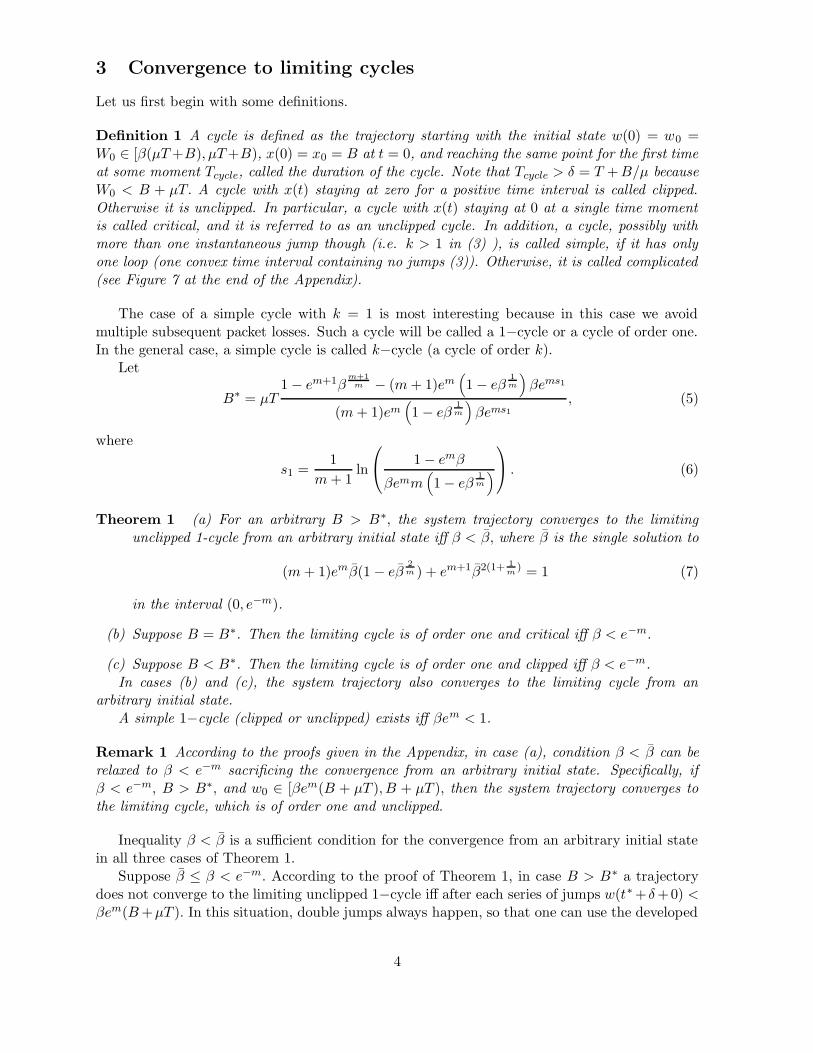
The proofs are presented in the Appendix.Secondly, consider the case B < B∗ and β < e−m. According to Theorem 1(c), all trajectories
converge to the clipped limiting 1−cycle; the phase portrait is presented in Figure 1.To calculate the main parameters λ, g, and x, we need the following quantities and functions.- Starting point of the cycle, i.e., the minimal value of w in Figure 1:
w0 = µTβem(SCD+1), (12)
where SCD is the single positive solution of
µT (emSCD + e−SCDm) − (m+ 1)(µT +B) = 0. (13)
6

-Duration of the cycle:
Tcycle =T
mln
1
β+B
µ
{
∫ SAB
0YAB(s)ds+
∫ SCD
0YCD(s)ds+ 1
}
, (14)
where SAB is the smaller positive solution of
0 = w0emSAB − µT (m+ 1) + e−SAB [(m+ 1)(B + µT ) − w0] ; (15)
here
YAB(s) =1
B(m+ 1)
{
w0ems − µT (m+ 1) + e−s [(B + µT )(m+ 1) − w0]
}
, s ∈ [0, SAB ], (16)
YCD(s) =µT
B(m+ 1)ems −
µT
B+ e−s
(
µTm
B(m+ 1)
)
, s ∈ [0, SCD]. (17)
2200 2250 2300 2350 2400 2450 2500 2550 2600 2650 2700
0
20
40
60
80
100
120
congestion window (packets)
buffe
r occ
upan
cy (p
acke
ts)
Instantaneouswindow reduction
D EA
B C
Figure 1: Clipped 1-cycle for Scalable TCP with µ = 1Gbps, T = 10ms, and B = 100pkts.Packet size is 4000 bits.
Proposition 2 The average sending rate is given by
λ =w0
Tcyclem
(
1
β− 1
)
, (18)
the average throughput is given by
g =1
Tcycle
{
w0
m(
1
βem− 1) + µT +B
}
, (19)
and the average amount of data in the buffer is given by
x =1
Tcycle
{
TB
(
∫ SAB
0YAB(s)ds+
∫ SCD
0YCD(s)ds
)
+B2
µ
(
∫ SAB
0Y 2
AB(s)ds+
∫ SCD
0Y 2
CD(s)ds
)
+B
(
T +B
µ
)
}
. (20)
7
The proofs are presented in the Appendix.According to Proposition 1, if B ≥ B∗ and the limiting 1-cycle is realized, then λ given by
(10) is strictly greater than µ and B-independent. Thus, (λ − µ) 6→ 0 as B → ∞. It meansthat in the MIMD case the rate of data loss in buffer overflow does not decrease as the buffersize increases. In contrast, in the AIMD case, we have (λ − µ) → 0 as B → ∞ [5]. Thissurprising result has the following explanation. In the MIMD case, when the cycle is unclippedboth the amount of data transfered over the cycle and the cycle duration are proportional toB + µT . For the parameters of the Slow Start phase of TCP New Reno with the DelayedAck mechanism (m = 0.5), the expression (10) gives (λ − µ)/µ ≈ 0.3. Fortunately, the SlowStart phase switches to the Congestion Avoidance phase after the first loss is detected by tripleduplicate acknowledgement [1]. According to (10), Scalable TCP induces as little as 0.1% losses.
According to Proposition 2, as B → 0, we have x → 0 and g → µ(βem − 1 −m)/ ln(β). Inparticular, in the case of Scalable TCP, we have g → 0.95µ as B → 0. We recall from [5] that forAIMD, when the packet size is small in comparison with the BDP (Bandwidth Delay Product)µT , we have g → µ(1+β)/2 as B → 0. Thus, the Congestion Avoidance phase of TCP New Renowith β = 0.5 has the worse link utilization of 0.75µ than that of Scalable TCP with β = 0.875(0.95µ) when the buffer size is small. It turns out that this difference mostly comes from differentvalues of β. In fact, one can easily check that µ(βem − 1 −m)/ ln(β) = µ(1 + β)/2 + o(1 − β)and consequently, if one chooses the same value of β close to one for AIMD and MIMD, the linkutilization would be the same for the two congestion control mechanisms for small buffer sizes.
5 Simulation results
We perform network simulations with the help of NS-2, the widely used open-source networksimulator [20]. We consider the following benchmark example of a TCP/IP network with a singlebottleneck link. The topology may for instance represent an access network. The capacity ofthe bottleneck link is denoted by µ and its propagation delay is denoted by d. We will considerseveral choices for the values of µ and d. The packet size is 500bytes = 4000bits. When wesimulate a scenario with multiple connections, we will assume that each connection is connectedto the bottleneck link via its own access link. The capacities of the access links are supposed tobe large enough so that they do not hinder the traffic.
We consider the MIMD control strategy with m = 0.01 and β = 0.875, that is, the standardvalues for Scalable TCP.
5.1 Impact of the buffer size on the link utilization
We first study how the utilization depends on the buffer size. We consider the values µ = 1Gbps= 1 Gigabit per second and d = 5ms (thus T = 2d = 10ms).
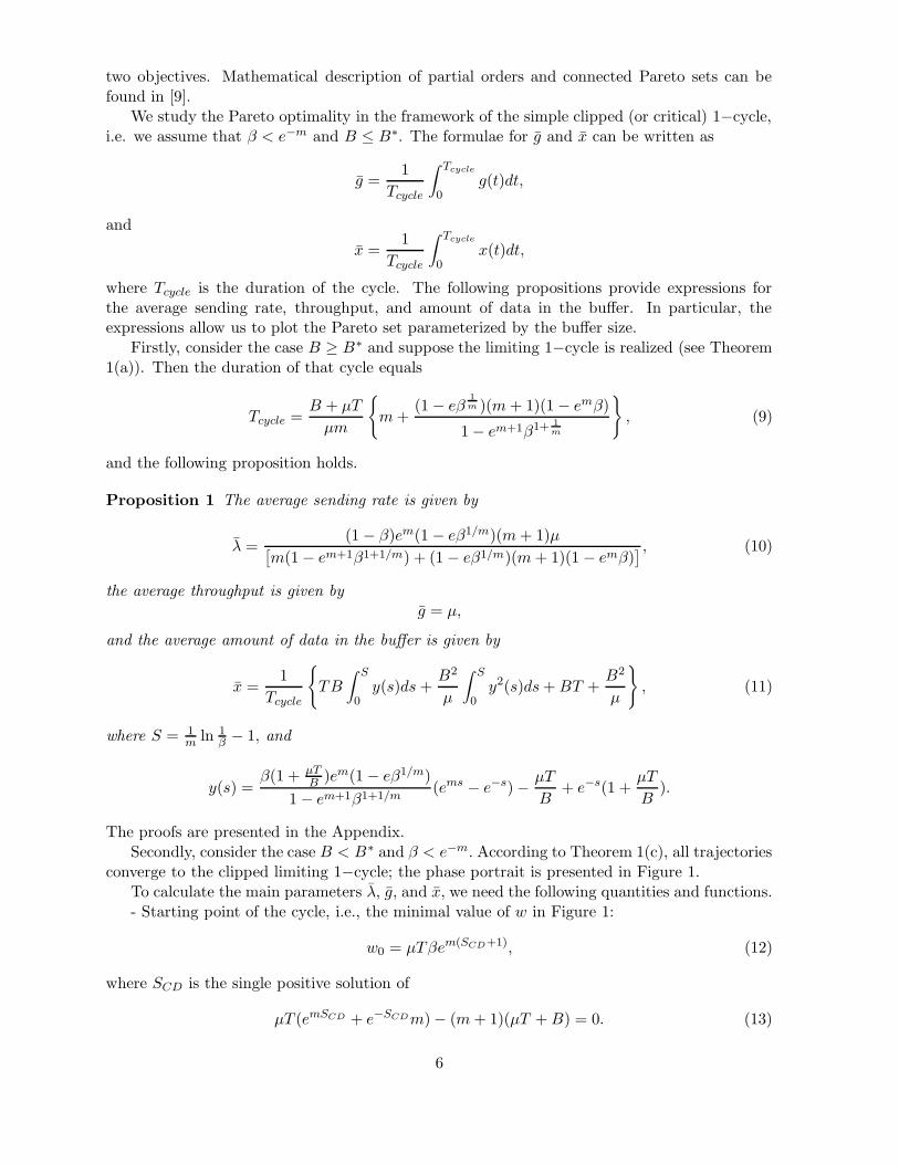
In Figure 2, based on our analytical results, we plot the value of B∗ (equation (5)) as afunction of m. We observe from Figure 2 that for m = 0.01, the value of B∗ is approximately230 packets (the packet size is 4000 bits).
We investigate the impact of the buffer size on the link utilization. From Theorem 1 itfollows that according to the fluid model, B∗ = 230 packets is the minimum buffer size suchas the link is utilized at 100%. Note that the BDP for these values is equal to 2500 packets.According to the well known rule of thumb for AIMD connections [27], the minimum buffer sizethat guarantees 100% utilization is 2500 packets.
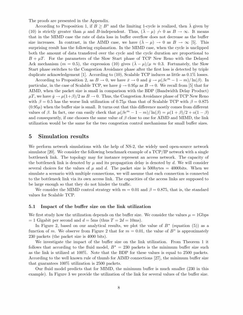
Our fluid model predicts that for MIMD, the minimum buffer is much smaller (230 in thisexample). In Figure 3 we provide the utilization of the link for several values of the buffer size.
8

0 0.02 0.04 0.06 0.08 0.10
50
100
150
200
250
300
350
mB
*
Figure 2: B∗ (in packets) as a function of m for Scalable TCP with µ = 1Gbps, T = 10ms, andβ = 0.875.
We note that in the simulation the minimum buffer size where we observe 100% utilization is 450packets. We note that the utilization when the buffer size is 230 packets is already quite highsince it is very close to 99%. Clearly our fluid model predicts a much smaller value, which canbe explained by the fact that the simulated traffic is not as smooth as it is in the fluid model.However we note that the fluid model estimation for B∗ is of the same order as the optimalvalue obtained via simulations when comparing it with the BDP rule-of-thumb for AIMD givenin [27].
150 200 250 300 350 400 450 5000.97
0.975
0.98
0.985
0.99
0.995
1
1.005
buffer size in packets
utili
zatio
n
Figure 3: Utilization against buffer size
5.2 Trajectories of the dynamical systems
We simulate now the evolution in time of the congestion window, the buffer occupancy and thesending rate. We consider the same example as above, namely, µ = 1Gbps = 1 Gigabit persecond and d = 5ms (thus T = 2d = 10ms). The packet size is 4000 bits. We consider againScalable TCP, that is, m = 0.01 and β = 0.875.
9

In Figures 4 and 5 we depict the curves of x(t), w(t) and λ(t) for B = 230 and B = 500,respectively. As predicted by Theorem 1, for B = 230, the cycle is critical, and the link is utilizedat 100%. For B = 500, the cycle is unclipped and the buffer does never empty. For B = 100, weplot the phase portrait of a clipped cycle in the plane (w, x) in Figure 1 for illustrative means.
0 0.1 0.2 0.3 0.4 0.5 0.6 0.7 0.8 0.9 10
50
100
150
200
250
time (sec)
buffe
r occ
upan
cy (p
acke
ts)
0 0.1 0.2 0.3 0.4 0.5 0.6 0.7 0.8 0.9 12400
2450
2500
2550
2600
2650
2700
2750
2800
time (sec)
cong
estio
n w
indo
w (p
acke
ts)
0 0.1 0.2 0.3 0.4 0.5 0.6 0.7 0.8 0.9 12.2
2.25
2.3
2.35
2.4
2.45
2.5
2.55
2.6x 10
5
time (sec)
send
ing
rate
(pac
kets
/sec
)
Figure 4: Evolution in time of the buffer occupancy, congestion window and sending rate forScalable TCP with µ = 1Gbps, T = 10ms, and B = 230pkts.
0 0.1 0.2 0.3 0.4 0.5 0.6 0.7 0.8 0.9 10
50
100
150
200
250
300
350
400
450
500
time (sec)
buffe
r occ
upan
cy (p
acke
ts)
0 0.1 0.2 0.3 0.4 0.5 0.6 0.7 0.8 0.9 12500
2600
2700
2800
2900
3000
3100
time (sec)
cong
estio
n w
indo
w (p
acke
ts)
0 0.1 0.2 0.3 0.4 0.5 0.6 0.7 0.8 0.9 12.2
2.25
2.3
2.35
2.4
2.45
2.5
2.55
2.6x 10
5
time (sec)se
ndin
g ra
te (p
acke
ts/s
ec)
Figure 5: Evolution in time of the buffer occupancy, congestion window and sending rate forScalable TCP with µ = 1Gbps, T = 10ms, and B = 500pkts.
The figures for sending rate λ(t) might appear a bit odd from the first glance. However,the flat part with the steep increasing part following it can be understood in the following way.Consider the derivative of λ with respect to t (corresponding to the part before x reaches buffer
size B). Based on equations (1, 2, 4), one can easily show that dλdt =
λ(m+1−λµ)
T+ xµ
. Now, focusing
on the numerator, clearly, dλdt = 0 when λ = µ(m + 1), as confirmed also by the figures. Say
λ(t) = µ(m+ 1). After this point t, we have a sliding mode, since λ > µ(m+ 1) ⇒ dλdt < 0 and
λ < µ(m + 1) ⇒ dλdt > 0. This sliding mode explains the flat part. On the other hand, this
motion is up to the point when x reaches B. Then as far as x stays there, dλdt = mλ
T+ Bµ
, explaining
the steep increasing part after the flat part.
5.3 Pareto set
Now we compare the numerical Pareto Set with the expressions for λ and g given in Propositions1 and 2. We consider AIMD (New Reno version [1]) and MIMD connections. In the case ofAIMD we will obtain the Pareto Set for several values of number of persistent connections,whereas for MIMD we will only consider one. We recall that several symmetric synchronizedMIMD connections are equivalent to a single MIMD connection.
10

Let N denote the number of persistent connections in the simulation. We will assume thateach connection is connected to the bottleneck link via its own access link. The capacities ofthe N access links leading to the bottleneck link are supposed to be large enough (or the loadon each access link is small enough) so that they do not hinder the traffic. For each of these Nlinks, the delay and capacity are di = 1ms and µi = 1000Mbps, respectively. The fact that thedelays in the access links are the same implies that the TCP connections will be synchronized.
We consider the following values for the bottleneck link: capacity is µ = 100Mbps, bottlenecklink propagation delay d = 1ms, the access link capacity and delay are 1000Mbps and 1ms,respectively. Thus T = 2(d+ di) = 0.004 sec.
In Figure 6 we depict the Pareto set for the cases of AIMD with N = 2, N = 5 and N = 20connections, and MIMD with just one connection. The qualitative shape of the curves agreeswith what our model predicts. In particular, MIMD achieves the full link utilization with amuch smaller buffer size than in the case of AIMD. We also display the theoretical trade-off
7.5 8 8.5 9 9.5 10
x 107
5
10
15
20
25
30
35
40
mean sending rate
mea
n qu
eue
leng
th
MIMD, N=1,MIMD, fluid model N=1AIMD, N=2AIMD, N=5AIMD, N=20
Figure 6: The trade-off curves for AIMD (N = 2, N = 5, N = 20, M = 1 packet = 500 bytes)and MIMD (N = 1, m = 0.01), β = 0.875, T = 0.004 sec, µ = 1000 Mbps.
curve for the mathematical fluid model as given in Propositions 1, 2. It turns to be close tothe curve coming from simulations. However, when comparing the results obtained from theanalytical model and from simulations we have observed some differences. For example, whenthe buffer size is zero, the simulated average sending rate is smaller than the one obtained withthe fluid model. Similarly, in the simulated scenario the minimal buffer size that guarantees thefull utilization of the link is larger than the one predicted by the fluid model. These differencescan be explained by the fact that the traffic in the simulations is not as smooth as the fluidmodel that we have used.
11

6 Conclusions
We have analyzed a hybrid model for the interaction between the MIMD congestion controlmechanism and a Drop Tail Internet router buffer. The present hybrid model is a significantextension of the model in [7]. The present model allows us to study the impact of the time-varying Round Trip Times on the system performance. We have obtained conditions for theabsence of multiple reductions of the congestion window within one congestion cycle. It turns outthat these conditions are violated in the Slow Start phase of TCP New Reno without the DelayedAck mechanism. Therefore, it is indeed recommended to use the Delayed Ack mechanism inthe Slow Start phase. Fortunately, the obtained conditions are satisfied by the parameters ofScalable TCP. For Scalable TCP, we construct the Pareto set that allows us to choose a buffersize which achieves a trade off between high link utilization and small queueing delays.
Acknowledgements
We would like to thank the three reviewers of the paper for their constructive and insightfulcomments. Their comments have been very valuable in preparing the revised version.
References
[1] M. Allman, V. Paxson and W. Stevens, TCP congestion control, RFC 2581, April 1999,available at http://www.ietf.org/rfc/rfc2581.txt.
[2] E. Altman, K. Avrachenkov, and B. Prabhu, et al “Queueing analysis of Scalable TCP”,in Computer Networks, 2005.
[3] G. Appenzeller, I. Keslassy and N. McKeown, “Sizing router buffers”, in Proc of ACMSIGCOMM ’04, Portland, Oregon, September 2004. Also in Computer CommunicationReview, Vol. 34, No. 4, pp. 281-292, October 2004.
[4] K. Avrachenkov, U. Ayesta and A. Piunovskiy, “Optimal choice of the buffer size in theInternet routers”, In Proc of IEEE CDC/ECC 2005, 2005.
[5] K. Avrachenkov, U. Ayesta and A. Piunovskiy, “Convergence and optimal buffer sizing forwindow based AIMD congestion control”, INRIA Research Report RR-6142. Available athttp://hal.inria.fr/inria-00136205/en/
[6] K. Avrachenkov, U. Ayesta, E. Altman, P. Nain, and C. Barakat, “The effect of routerbuffer size on the TCP performance”, in Proc of LONIIS workshop, St. Petersburg, Jan. 29- Feb. 1, 2002.
[7] U. Ayesta, A. Piunovskiy and Y. Zhang, “Fluid model of an Internet router under the MIMDcontrol scheme”, in Telecommunications Modeling, Policy and Technology (S.Raghavan,B.Golden and E.Wasil - eds.), Springer, NY, 2008, pp.239-251.
[8] S. Bohacek, J.P. Hespanha, J. Lee, and K. Obraczka, “A hybrid systems modeling frame-work for fast and accurate simulation of data communication networks”, in Proc of ACMSIGMETRICS 2003, 2003.
[9] G.Dorini, F.Di Pierro, D.Savic, and A.B.Piunovskiy, “Neighbourhood search for construct-ing Pareto sets”, Math. Meth. Oper. Res., v.65, pp.315-337, 2007.
12

[10] R. El Khoury and E. Altman, “Analysis of Scalable TCP”, in Proceedings of HET-NET,2004.
[11] M. Enachescu, Y. Ganjali, A. Goel, N. McKeown and T. Roughgarden, “Part III: Routerswith Very Small Buffers”, ACM SIGCOMM Computer Communication Review, v. 35(2),pp. 83-90, 2005.
[12] S. Floyd, “HighSpeed TCP for Large Congestion Windows”, RFC 3649, December 2003,available at http://www.ietf.org/rfc/rfc3649.txt.
[13] S. Gorinsky, A. Kantawala, and J. Turner, “Link buffer sizing: a new look at the oldproblem”, in Proc of IEEE Symposium on Computers and Communications (ISCC 2005),June 2005.
[14] J.P. Hespanha, S. Bohacek, K. Obraczka, and J. Lee, “Hybrid modeling of TCP congestioncontrol”, In Hybrid Systems: Computation and Control, LNCS v.2034, pp.291-304, 2001.
[15] V. Jacobson, Congestion avoidance and control, ACM SIGCOMM’88, August 1988.
[16] C. Jin, D.X. Wei, and S.H. Low, “FAST TCP: Motivation, Architecture, Algorithms, Per-formance”, in Proc. IEEE INFOCOM, 2004.
[17] T. Kelly, “Scalable TCP: Improving performance in highspeed wide area networks”, Com-puter Comm. Review, v.33, no.2, pp.83-91, 2003.
[18] D.J.Leith and R.N.Shorten, “H-TCP Protocol for High-Speed Long-Distance Networks”,in Proc. 2nd Workshop on Protocols for Fast Long Distance Networks. Canada, 2004.
[19] Y.Li, D.J.Leith and R.N.Shorten, “Experimental Evaluation of TCP Protocols for High-Speed Networks”, IEEE/ACM Transactions on Networking, v.15, issue. 5, pp. 1109-1122,2007.
[20] “Network Simulator, Ver.2, (NS-2) Release 2.18a”, Available at:http://www.isi.edu/nsnam/ns/index.html.
[21] A.B. Piunovskiy, Optimal Control of Random Sequences in Problems with Constraints.Kluwer Academic Publishers: Dordrecht, 1997.
[22] R. Prasad, C. Dovrolis and M. Thottan, “Router Buffer Sizing Revisited: The Role of theOutput/Input Capacity Ratio”, in Proceedings of ACM CoNext 2007.
[23] G. Raina, D. Towsley and D. Wischik, “Part II: Control Theory for Buffer Sizing”, ACMSIGCOMM Computer Communication Review, v. 35 (3), pp. 79-82, 2005.
[24] G. Raina and D.J. Wischik, “Buffer sizes for large multiplexers: TCP queueing theory andinstability analysis”, in Proceedings of EuroNGI, Rome, April 2005.
[25] I. Rhee and L. Xu, “CUBIC: A new TCP-friendly High-Speed TCP variant”, in Proceedingsof PFLDnet 2005 workshop, February 2005.
[26] R. Stanojevic, R. Shorten and C. Kellet, “Adaptive tuning of Drop-Tail buffers for reducingqueueing delays”, IEEE Communications Letters, v.10(7), July, 2006.
[27] C. Villamizar and C. Song, “High Performance TCP in the ANSNET”, ACM SIGCOMMComputer Communication Review, v.24, no.5, pp.45–60, November 1994.
13

[28] G. Vu-Brugier, R.S. Stanojevic, D. J. Leith, and R.N. Shorten, “A critique of recentlyproposed buffer-sizing strategies”, ACM SIGCOMM Computer Communication Review,v.37(1), pp.43-48, 2007.
[29] D. Wischik and N. McKeown, “Part I: Buffer Sizes for Core Routers”, ACM SIGCOMMComputer Communication Review, v. 35(2), pp. 75-78, 2005.
[30] L. Xu, K. Harfoush and I. Rhee “Binary Increase Congestion Control for Fast Long-DistanceNetworks”, in Proceedings of IEEE INFOCOM 2004, 2004.
Appendix
The Appendix is organized as follows. Firstly, we prove a series of Lemmas and then use themto prove Theorem 1. The proofs of Propositions 1, 2 come at the end.
To make the model more tractable, we change the time scale and the variables as follows.
ds =dt
T + x(t)/µ, y = x/B, and v = w/B.
Thendv
ds=dv
dw
dw
dt
dt
ds=mw(s)
B= mv(s), (21)
and
dy
ds=
dydx
dxdt
dtds = v(s) − q − y(s) if 0 < y(s) < 1, or y(s) = 0 and v(s) > q,
or y(s) = 1, and v(s) ≤ q + 10 otherwise,
(22)
where we have put q = µTB , which is a positive constant. Now everything is in the new time
scale. Let s∗ be the time moment in the new time scale when the state of the system reaches 1.That is, y(s∗) = 1. Then the impulsive control (3) can now be written as
v(s∗ + 1 + 0) = βkv(s∗ + 1 − 0), (23)
where k = min{i = 1, 2, . . . : βiv(s∗ + 1 − 0) < q + 1}, and we notice that the time delay δ hasbeen standardized in the new time scale. With the new variables and time scale, we see whenthe buffer is filled full, y(s∗) reaches 1, after 1 RTT, the congestion signal is received leadingto a multiplicative reduction on v(s∗) with a factor βk, where k is just defined above. Note,reducing v below q+1 = µT
B +1 exactly corresponds to reducing the instantaneous sending rate
defined as v(∗)BT+ µ
Bbelow the capacity µ.
If we ignore the non-negativity constraint on variable y, then one can solve (21) and (22) forv(s) and y(s) with initial conditions v(0) = v0 and y(0) = y0 respectively, and obtain
v(s) = v0ems (24)
y(s) =v0
m+ 1ems − q + e−s
(
y0 + q −v0
m+ 1
)
, (25)
and the existence and uniqueness of the above two solutions follow from the initial value problemsof ordinary differential equations.
With the new variables in the new time scale, we give a corresponding version of Definition1 as follows.
14
Definition 1’ A cycle is defined as the trajectory starting with the initial point (a particularV0 ∈ [β(q + 1), q + 1), y(0) = y0 = 1) at s = 0, and reaching the same point for the first timeat some S + 1 ≥ 1. And S + 1 is called the duration of the cycle. A cycle with y(s) stayingat zero for a positive time interval is called clipped. Otherwise it is unclipped. In particular, acycle with y(s) staying at 0 at a single time moment is called critical, and it could be referredto as an unclipped cycle. In addition, cycles, possibly with more than one instant jump though,are called simple, if they have only one loop. Otherwise, they are called complicated.
In what follows, expression “unconstrained case” means that we ignore the non-negativityconstraint on variable y. Expression “general case” means that we impose constraint y ≥ 0.Under “trajectory” we mean the phase portrait y(s) against v(s): see Figure 1.
Lemma 1 In the unconstrained case, 1-cycle exists iff βem < 1.
Proof. Consider the unconstrained case. A 1−cycle exists iff there exists a nonnegative numberV0 such that V0 ∈ [β(q + 1), q + 1), and
βV0em(S+1) = V0 (26)
1 =V0
m+ 1emS − q + e−S
(
1 + q −V0
m+ 1
)
, (27)
where we have already put y0 = 1.Firstly one can check the existence of a solution to equations (26) (27). Indeed from (26) we
have
S =1
mln
1
β− 1, (28)
so that (27) results in
V0 =(1 + q)emβ
(
1 − eβ1m
)
(m+ 1)
1 − em+1β(1+ 1m)
. (29)
Secondly, one can check that V0 given by equation (29) is in the interval [β(q + 1), q + 1),provided 1 + q > 0 and β ∈ (0, e−m). The latter condition is necessary and sufficient for thepresented reasoning to hold.
In what follows, it is assumed that emβ < 1.
Lemma 2 Consider the unconstrained case. Starting from an arbitrary initial state v0 ∈ (0, 1+q), y0 = 1, component y(s) attains its single minimum at the moment
s1(v0) =1
m+ 1ln
(1 + q)(1 +m) − v0
mv0> 0. (30)
The value y(s1) increases with v0 and y(s1) → 1 as v0 → 1 + q.A 1−cycle is critical for a single nonnegative value of q given by
q∗ =(m+ 1)em
(
1 − eβ1m
)
βems∗1
1 − em+1βm+1
m − (m+ 1)em(
1 − eβ1m
)
βems∗1, (31)
where s∗1 = s1(V∗
0 ) = 1m+1 ln
1−emβ
βemm
(
1−eβ1m
)
, and V ∗
0 is given by (29) with q = q∗.
In the general case (if we impose constraint y ≥ 0) the 1−cycle is unclipped iff q ≤ q∗.
15

Proof. According to equations (24) (25), we have the following equations satisfied by s1(v0):
v(s1) = v0ems1
y(s1) = v0m+1e
ms1 − q + e−s1(1 + q − v0m+1)
y(s1) = v(s1) − q.
Solving them for s1 gives (30), and
y(s1(v0)) =
(1 + q)(1 +m)v1m0 − v
1+mm
0
m
mm+1
− q.
One can easily check that y(s1(v0)) → 1 as v0 → 1 + q. For dy(s1(v0))dv0
, we have
dy(s1(v0))
dv0=
m
m+ 1
(1 + q)(1 +m)v1m0 − v
1+mm
0
m
−1m+1
×
{
1 +m
m2v
1m−1
0 (1 + q − v0)
}
> 0.
Let us fix an arbitrary q > 0 and consider the corresponding simple 1−cycle with thecorresponding value of V0 defined in (29). Now
s1(V0) =1
m+ 1ln
1 − emβ
memβ(1 − eβ1/m)= s∗1 (32)
and according to (22) and (24)
y(s1(V0)) = v(s1) − q = V0ems1 − q.
Since s1 is q−independent, y(s1(V0)) is a linear function of q. Let us show that it decreaseswith q.
Indeed, if q → 0 then y(s1(V0)) has a positive limit. When q increases, y(s1(V0)) becomesnegative. To see this, notice that at the beginning of the cycle, starting from v(0) = V0 < 1 + q,y(0) = 1, component y decreases. Moreover,
d
ds
(
y(s)
q
)∣
∣
∣
∣
s=0
=V0
q− 1 −
1
q→
emβ(1 − eβ1/m)(m+ 1)
1 − em+1β1+1/m− 1
as q → ∞.And the latter expression is negative because emβ(1−eβ1/m)(m+1)−1+em+1β1+1/m <
0 for β ∈ (0, e−m). Therefore, y(s)q decreases with time s, when s is small, at large values of q,
starting from initial value y0
q = 1q , meaning that y(s)
q takes negative values if q is sufficiently big,i.e. the minimal value, y(s1) < 0.
Therefore, there exists a single value q∗ > 0 such that y(s1(V0)) = 0. Clearly, the lastequality holds iff
V ∗
0 ems∗1 − q∗ =
(1 + q∗)emβ(1 − eβ1/m)(m+ 1)
1 − em+1β1+1/mems∗1 − q∗ = 0.
It only remains to solve the equation obtained for q∗.The last statement is obvious.
16

Remark 2 According to (29)
dV0
dβ=
(1 + q)em(m+ 1)[1 − e(1 + 1m )β1/m − em+1β1+1/m + em+1(1 + 1
m )β1+1/m]
(1 − em+1β1+1/m)2,
and the standard analysis of the derivatives shows that the latter function of β is positive ifβ ∈ (0, e−m). Trajectories (v(s), y(s)) cannot cross when starting from different initial points(v(0) = V 1
0 , y(0) = 1) and (v(0) = V 20 , y(0) = 1); thus the minimal value y(s1(V0)) increases
with β.
Corollary 1 In the general case, where constraint y(s) ≥ 0 is imposed, if a trajectory startingwith some v0 ∈ (0, 1 + q) is clipped, there will be some v0 ∈ (v0, 1 + q), starting with whichthe trajectory just touches the horizontal v axis, i.e., y(s1(v0)) = 0. Furthermore, trajectoriesstarting with v0 ∈ [v0, 1 + q) are unclipped, while those with v0 ∈ (0, v0) are clipped. As a result,if q ≤ q∗, V0 ≥ v0, where V0 is given by (29).
Proof. Everything follows directly from the first part of Lemma 2, bearing in mind that increasingy(s1(v0)) is a continuous function of v0.
After the continuous trajectory starting with v(0) = v0 < 1 + q and y(0) = 1 finishes, thatis, the buffer is filled up and the congestion is noticed after the delay, there will be a reductionon the variable v leading to v1 ∈ [β(1 + q), 1 + q). Therefore, as the process proceeds, we havea sequence {vi}. If this sequence has a limit, namely v∞, a limiting cycle exists and will berealized.
According to (24) and (25), we introduce the following denotations (for v < 1 + q):
ϕ(v) = βvem(s+1), (33)
where s > 0 solves equation
F (v, s) =v
m+ 1
(
ems − e−s)+ (1 + q)(
e−s − 1)
= 0. (34)
In the unconstrained case, (or if an actual continuous trajectory is unclipped), if only one jumpis sufficient, vi+1 = ϕ(vi). We shall also use the denotation ψ(v) = ϕ(ϕ(v)) = ϕ2(v) for brevity.
Note that, if the actual continuous trajectory starting from v(0) = v, y(0) = 1 is clippedthen, at the next time moment s∗ when y(s∗) = 1, v(s∗) < vems implying v(s∗ + 1 + 0) < ϕ(v)provided only one jump is sufficient in the unconstrained case.
Lemma 3 In the unconstrained case, starting with an arbitrary v0 ∈ [βem(1 + q), 1 + q), thelimiting simple cycle exists and is of order one.
Proof. One can check that there exists only one s > 0 solving (34) for v ∈ (0, 1 + q). Itis convenient to investigate the mapping ϕ defined on the closed segment [βem(1 + q), 1 +q]: ϕ(1 + q) = βem(1 + q). (Equation (34) has only one zero solution for v = 1 + q andlimv→1+q−0 ϕ(v) = βem(1 + q).)
Our proof will be performed in three steps:
1. ϕ(v) decreases with v. Hence ψ(v) increases with v. This statement holds for all v ∈(0, 1 + q).
2. ϕ : [βem(1+q), 1+q] → [βem(1+q), 1+q] and ψ : [βem(1+q), 1+q] → [βem(1+q), 1+q].
17

3. {ϕn(v)} and {ψn(v)} both converge to v∞ ∈ [βem(1 + q), 1 + q).
For item 1, according to implicit differentiation and partial differention,
dϕ(v)
dv=
βe−s(m+ 1)em(s+1)(v − (q + 1))
v (mems + e−s) − (m+ 1)(q + 1)e−s, (35)
where the numerator of the last expression is smaller than zero for v < 1 + q.The denominator of the last expression equals
v(
emsm+ e−s)− (m+ 1)(q + 1)e−s =(1 + q)(m+ 1)e−s
ems − e−sG1(s),
where G1(s) = me(m+1)s −mems +1− ems. (We have put in v = (1+q)(1−e−s)(m+1)ems−e−s , according to
equation (34).) Finally, G1(s) > 0 for s > 0.For item 2, we consider v ∈ [βem(1+q), 1+q). According to item 1, ϕ(1+q) and ϕ(βem(1+
q)) give a lower and an upper bounds for ϕ(v), respectively. We then need to show that ϕ(1+q) ≥βem(1 + q) > β(1 + q), and ϕ(βem(1 + q)) < 1 + q. Since ϕ(1 + q) = βem(1 + q), it remains toprove that ϕ(βem(1 + q)) ≤ 1 + q.
According to (34), where we put in v = βem(1 + q), we have
(1 + q)βem
m+ 1
(
ems − e−s)+ (1 + q)(
e−s − 1)
= 0 ⇔ G2(s, β,m) = 0,
where G2(s, β,m) = βem (ems − e−s) + (m+ 1) (e−s − 1). Function G2(s, β,m) firstly decreaseswith respect to s from zero and then increases up to ∞ after the single minimum point, resultingin a single positive solution s solving (34) with v = βem(1 + q).
Clearly, ϕ(βem(1+q)) = β2(1+q)emem(s+1), where s solves (34) with v = βem(1+q). Definethe increasing (with respect to s) auxiliary function G3(s) = β2(1+q)emem(s+1). We aim to showthat, for s satisfying G3(s) = 1+q, i.e., s(β,m) = 2
m ln 1β −2, G2(s(β,m), β,m) > 0. That would
say, s(β,m) is greater than the solution of (34) with v = βem(1+ q), and ϕ(βem(1+ q)) < 1+ q.We have
G2(s(β,m), β,m) = (emβ)−1 − βem(
eβ1m
)2+ (m+ 1)
(
(
eβ1m
)2− 1
)
= G2(β,m).
Observe that G2(β,m) → ∞ as β → 0 and G2(β,m) → 0 as β → e−m.Furthermore,
∂G2(β,m)
∂β= e−mβ−2G3(β,m),
where G3(β,m) = −1 − m+2m e2m+2β
2m+2m + 2(m+1)
m em+2β2+m
m < 0 for β ∈ (0, e−m). Therefore,∂G2(β,m)
∂β < 0 ⇒ G2(β,m) > 0 ⇔ G2(s(β,m), β,m) > 0, as required.It follows from item 1 that starting with an arbitrary v ∈ [βem(1 + q), 1 + q), {ψn(v)} is
a monotonic sequence. It follows from item 2 that the sequence {ψn(v)} is bounded in theclosed interval [βem(1 + q), 1 + q]. Hence, ψn(v0) → v∞ = ψ(v∞) ∈ [βem(1 + q), 1 + q] asn → ∞. It also follows from item 2 that with emβ < 1, exactly one jump is enough, startingwith v ∈ [βem(1 + q), 1 + q).
For item 3, assume ϕ(v∞) = v′∞
6= v∞. Let S2 and S3 be such that
0 =v′∞
m+ 1
(
emS2 − e−S2
)
+ (1 + q)(
e−S2 − 1)
(36)
18

0 =v∞
m+ 1
(
emS3 − e−S3
)
+ (1 + q)(
e−S3 − 1)
. (37)
Then S2 + 1 and S3 + 1 are the durations of continuous trajectories starting with v ′∞
and v∞,respectively. (See (34).) Then by the definition of v∞,
v∞ = ββv∞em(S3+1)em(S2+1),
leading to
β = e−12m(S2+S3+2). (38)
By the definition of v′∞
, we have v′∞
= βv∞em(S3+1). But from (36) we have in parallel v′
∞=
(1+q)(m+1)(1−e−S2 )emS2−e−S2
. If we substitute expression for v∞ coming from (37), and use formula (38),we see that
(1 − e−S2)e12mS2
emS2 − e−S2=
(1 − e−S3)e12mS3
emS3 − e−S3. (39)
One can show that function (1−e−z)e12
mz
emz−e−z strictly decreases if z > 0. Hence S2 = S3 and
v′∞
= v∞ < 1+ q because ϕ(1+ q) = βem(1+ q) 6= 1+ q. Therefore, ϕn(v0) → v∞ as n→ ∞.
Remark 3 It follows from item 3 in the proof of Lemma 3 that in the unconstrained case,starting with an arbitrary v0 ∈ [βem(1+ q), 1+ q), complicated cycles cannot be realized, and v∞coincides with V0 given by (29).
Corollary 2 −1 < dϕ(v0)dv0
∣
∣
∣
V0
< 0, so that the mapping ϕ is a contraction in a neighborhood of
the stable point V0.
Proof. By putting in V0 given by (29) and S given by (28) into (35), we have dϕ(v)dv
∣
∣
∣
V0
=
eβ1/m[(m+1)emβ−1−mem+1β1+1/m](1−eβ1/m)m+em+1β1+1/m
−eβ1/m . We already know that dϕ(v)dv < 0 (see item 1 above). Hence we
just need to prove that dϕ(v0)dv0
∣
∣
∣
V0
> −1 ⇔ P1(β,m) > 0, where P1(β,m) = (m + 1)emβ − 2 −
mem+1β1+m
m + emβ −m +m(eβ1m )−1. But the standard analysis of the derivatives shows that
function P1(β,m) monotonically decreases from ∞ to 0 for β ∈ (0, e−m).
Corollary 3 In the unconstrained case, let v0 ∈ [βem(1 + q), 1 + q). Then ∀i ∈ {0, 1, 2, . . .}vi ∈ [βem(1 + q), 1 + q), and vi+2 ∈ [min(vi, vi+1),max(vi, vi+1)].
Proof. The first statement follows from the proof of Lemma 3.Without loss of generality, we can put i = 0. That is, we aim to show that
v2 ∈ [min(v0, v1),max(v0, v1)]. According to item 2 in the proof of Lemma 3, vi = ϕ(vi−1).Consider the case v0 > v1. Automatically we have v2 > v1, since ϕ is decreasing. Then thereare two possibilities about the relationship between v0, v1, and v2:
1. v2 > v0 > v1.
2. v2 ∈ [v1, v0].
Suppose the first possibility is true, that is, v2 > v0 > v1. We aim to show by induction thatin this case, v2i+2 > v2i > . . . > v2 > v0 > v1 > . . . > v2i+1, ∀i ∈ {0, 1, 2, . . .}. These inequalitieshold for i = 0. Suppose they hold for some i ≥ 0. Consider the case i + 1. From the induction
19

supposition we have v2i+2 > v2i. Therefore v2i+1 > v2i+3, and v2i+4 > v2i+2. Hence sequence{vi} does not converge which contradicts Lemma 3.
Therefore, the first possibility is false. And v2 ∈ [v1, v0] holds automatically, as we want.Exactly in the same manner, one can show that in the case v0 < v1, v2 ∈ [v0, v1]. And the casev0 = v1 is trivial. Hence, v2 ∈ [min(v0, v1),max(v0, v1)], as required.
Remark 4 According to Corollary 1 and Corollary 3, in the general case, starting with v ∈[βem(1 + q), 1 + q), once two consecutive unclipped trajectories are realized, all the subsequenttrajectories will be unclipped.
Lemma 4 Under the main assumption of emβ < 1, the trajectory starting with v(0) = v0 =β(1 + q), y(0) = 1 requires no more than two jumps.
Proof. Suppose the trajectory is unclipped. Starting with v0 = β(1+q), let us examine the valueof βϕ(β(1 + q)) = β3(1 + q)em(s+1), where s is the single positive solution to L(s, β,m) = 0,where L(s, β,m) = β(ems − e−s) + (m+ 1)(e−s − 1) according to (34). Hence, β3(1 + q)em(s+1)
is the value of v1 after two instant jumps, if starting with v0 = β(1 + q). Define the increasing(with respect to s) auxiliary function C(s) = β3(1 + q)em(s+1). One can easily check that thebehaviour of L(s, β,m) is similar to that of G2(s, β,m) in the proof of Lemma 3, in the sensethat it decreases firstly from zero and then increases up to infinity, with respect to s.
Let us show that L(s(β,m), β,m) > 0, where s(β,m) is the single positive solution toC(s) = 1 + q: s(β,m) = − 3
m lnβ − 1.Now
L(s(β,m), β,m) = β−2e−m − β3+m
m e+ (m+ 1)(β3m e− 1).
Immediately L(s(β,m), β,m) → ∞ as β → 0. And as β → e−m, L(s(β,m), β,m)→ em − e−2−m + (m + 1)(e−2 − 1) > 0, as can be verified easily. Now one can calculatethe partial derivative
∂L(s(β,m), β,m)
∂β= −2β−3e−m −
m+ 3
mβ
3m e+ (m+ 1)
3
mβ
3m−1e.
Immediately ∂L(s(β,m),β,m)∂β → −∞ as β → 0, and one can show that
limβ→e−m
(
∂L(s(β,m), β,m)
∂β
)
= −2e2m −3 +m
me−2 +
3(m+ 1)
mem−2 < 0
for any m > 0.
Finally, the analysis of the second order derivative implies ∂2L(s(β,m),β,m)∂β2 > 0, so that
L(s(β,m), β,m) > 0.Hence s < s(β,m) and C(s) < 1 + q meaning that βϕ(β(1 + q)) < 1 + q.If the trajectory is clipped then the value after the next two instantaneous jumps is even
smaller than βϕ(β(1 + q)).
Corollary 4 If emβ < 1 then no-one cycle has more than two instantaneous jumps.
Proof. It is sufficient to notice that, after any instantaneous series of jumps, v ≥ β(1 + q) andβϕ(v) ≤ βϕ(β(1 + q)).
Lemma 5 In the unconstrained case, 2−cycles are absent iff β < β, where β is the singlesolution in the interval (0, e−m) to equation (7).
20

Proof. Clearly a 2−cycle, described by the starting point
V(2)0 =
(1 + q)emβ2(
1 − eβ2m
)
(m+ 1)
1 − em+1β(2+ 2m )
,
does not exist iffV
(2)0β < 1 + q. (Compare with the proof of Lemma 1.) Or equivalently,
Q1(β) = (m+ 1)emβ(1 − eβ2m ) + em+1β2(1+ 1
m) < 1.
The standard analysis of the derivatives implies that Q1(β) increases with β from Q1(0) = 0and, after a single stationary point, decreases up to Q1(e
−m2 ) = 1. Therefore, equation (7) has
a single solution in interval (0, e−m2 ) ⊃ (0, e−m).
One can easily check that
V(2)0
β
∣
∣
β=e−m > 1 + q, (40)
which is equivalent to β < e−m.
Remark 5 Suppose β < e−m. Then, in the general case, 2−cycles exist for some (big enough)values of B iff β ≥ β. According to Lemma 1, 1−cycles also exist. What is actually realized,depends on the initial conditions v(0) = v0, y(0) = 1.
Lemma 6 In the unconstrained case, the continuous trajectory starting from v(0) = v0 = β(1+q), y(0) = 1 reaches level y(s) = 1 with such a value of v(s) that βv(s+ 1) < 1 + q if and only ifβ < β.
Proof. Clearly βv(s + 1) = ϕ(v0) = β2(1 + q)em(s+1), where s > 0 solves equation (34) atv = v0 = β(1 + q). Now βv(s+ 1) < 1 + q ⇔ β2em(s+1) < 1.
Firstly, one can check that equations
β2em(s+1) = 1; (41)
β(ems − e−s) + (m+ 1)(e−s − 1) = 0 (42)
hold iff β = β. Indeed, substitute expression s = −2 lnβm − 1 obtained from (41), into (42):
β(e−m
β2− eβ2/m) + (m+ 1)(eβ2/m − 1) = 0 ⇔ (7) ⇔ β = β.
Secondly, from (42) we obtain
ds
dβ=
ems − e−s
(m+ 1)e−s − β(mems + e−s).
The numerator is positive for s > 0. After we substitute β = (1−e−s)(m+1)ems
−e−s , obtained from (42),into the denominator, we obtain
(m+ 1)e−s(ems − e−s) − (1 − e−s)(m+ 1)(mems + e−s)
ems − e−s< 0
because ems−s −mems +mems−s − e−s < 0 at any positive s and m. (The latter inequality canbe established when analysing the lefthand part as function of m ∈ (0,∞).) Thus ds
dβ < 0.
21

Finally, we intend to prove that limβ→0 β2em(s+1) = 0. When β → 0, s increases, but the limit
cannot be finite. (Otherwise, passing to the limit in (42) would imply (m+1)(e− limβ→0 s−1) = 0.)Hence limβ→0 s = ∞, and from (42) we have limβ→0 βe
ms = m + 1 ⇒ limβ→0 β2em(s+1) = 0.
Therefore, β2em(s+1) < 1 ⇔ β < β because β is the single value of β providing β2em(s+1) = 1,and the lefthand side is obvioulsy a continuous function of β.
Proof of Theorem 1. Note that β is the single solution to equation (7) in the interval(0, e−m) according to Lemma 5. If β < e−m Lemma 4 excludes trajectories with three or moreinstantaneous jumps (perhaps after one first continuous trajectory is realised).
(a) Suppose β < β and B ≥ B∗ ⇔ q ≤ q∗. Lemma 6 implies that (perhaps after the first oneinstantaneous series of jumps) multiple reductions of component v never occur and all the furthervalues of vi belong to [βem(1 + q), 1 + q). For the proof of the latter statement, remember thedenotations introduced before Lemma 3, and equality ϕ(1+q) = βem(1+q). Even if a continuoustrajectory starting from v(0) = vi, y(0) = 1 is clipped, vi+1 = ϕ(v0) ∈ [βem(1 + q), 1 + q), wherev0 was defined in Corollary 1.
Suppose there exists a clipped continuous trajectory starting from v(0) = vi, y(0) = 1.(Actually, i can equal 1 or 2.) The next trajectory starting from v(0) = vi+1 ∈ [βem(1 + q), 1 +q), y(0) = 1 cannot be clipped because otherwise we would have obtained a clipped 1−cyclewhich contradicts the last statement of Lemma 2. Thus vi+1 ≥ v0 and vi+2 = ϕ(vi+1). Sincevi+1 = ϕ(v0), we can use Corollary 3: vi+2 ≥ v0, so that trajectory starting from v(0) =vi+2, y(0) = 1 is also unclipped. According to Remark 4, all the subsequent trajectories areunclipped and converge to the limiting unclipped 1−cycle in accordance with Lemma 3.
If β ≥ β then, according to Remark 5, statement (a) is false.All the presented reasoning holds also if β ≤ β < e−m and v0 ∈ [βem(1+ q), 1+ q) : multiple
jumps never occur and ∀i ≥ 0 vi ∈ [βem(1+q), 1+q). (See the proof of Lemma 3.) On the otherhand, according to Remark 5, for some initial conditions, a simple 2−cycle can be realized if Bis big enough. This observation justifies Remark 1.
(b) If B = B∗, the previous paragraph is correct, but (independently of the initial state)no-one continuous trajectory can have multiple jumps at the end, because it cannot be situatedbelow the curve starting from v(0) = q, y(0) = 0 which results in the single jump at the end.Thus, trajectories converge to the 1−cycle that is critical according to Lemma 2. The necessityof inequality β < e−m can be proved similarly to the part (c).
(c) Similarly to case (b), continuous trajectories having multiple jumps at the end cannot berealized if B < B∗ ⇔ q > q∗. According to Lemma 2, one cannot meet an unclipped 1−cycle.Corollary 1 and Lemma 3 imply that v0 ∈ [βem(1 + q), 1 + q). Moreover, ϕ(v0) < v0 becauseotherwise, starting from v(0) = v0, y(0) = 1 we would have had two consecutive unclippedtrajectories leading to an unclipped limiting 1−cycle according to Remark 4 and Lemma 3.
Now one of the following two scenarios can take place.If v0 < v0, then the first continuous trajectory is clipped and v1 = ϕ(v0) < v0, so that the
next continuous trajectory is also clipped, and the limiting clipped 1−cycle is attained after oneiteration.
If v0 ≥ v0, then the first continuous trajectory is unclipped, but v1 = ϕ(v0) < v0. (Otherwisewe face two consecutive unclipped trajectories leading to the existence of an unclipped 1−cycle.)Hence v1 gives a clipped continuous trajectory, and, according to the previous paragraph, wefinish with the clipped 1−cycle attained after two iterations.
As Lemma 1 says, an unclipped 1−cycle does not exist if βem < 1. One can easily show thatinequality βem < 1 is also necessary for the existence of clipped 1−cycles. Indeed, if βem ≥ 1then formula (28) gives S ≤ 0, and that formula remains the same for clipped and unclipped
22

cycles because equation (26) is universal.The very last statement is justified in full by all the previous reasoning.
Before proving Proposition 1, let us justify formula (9). Clearly,
Tcycle =
∫ Tcycle
0dt =
∫ S+1
0
{
T +By(s)
µ
}
ds,
where S is given by (28), and expression (9) follows.Proof of Proposition 1. In the case q ≤ q∗ ⇔ B ≥ B∗ = µT
q∗ , the cycle is unclipped. The av-
erage sending rate can be calculated according to formula λ =
∫ S+1
0w(s)ds
Tcycle= B
Tcycle
∫ S+10 V0e
msds
(see (24)). The average throughput can be calculated as the following.
g =1
Tcycle
{
∫ Tcycle−T−Bµ
0λ(t)dt+ µ
(
T +B
µ
)
}
=1
Tcycle
{
∫ S
0w(s)ds+ µ
(
T +B
µ
)
}
= µ.
Also, the average amount of data in the buffer is calculated as below.
x =1
Tcycle
∫ Tcycle
0x(t)dt =
1
Tcycle
∫ S+1
0By(s)(T +
By(s)
µ)ds.
In case B < B∗ ⇔ q > q∗, the cycle is clipped. As before, we use t(s) for the original (new)time scale. The graph of the cycle in the plane (v, y) looks similarly to Figure 1; one has onlyto replace “Buffer size (B)” on the y−axis by 1. Suppose the cycle starts at s = SA = 0 frompoint A, reaches point B at time moment SB and so on. We shall use denotations like SBC forSC − SB.
Point C has coordinates y = 0 and v = q, so that, when s ∈ [SC , SD],
y(s) =q
m+ 1em(s−SC ) − q + e−(s−SC)(
mq
m+ 1)
according to (25). Therefore, SCD = SD−SC is the single positive solution to equation A(s) = 0where
A(s) = qems + e−sqm− (m+ 1)(q + 1).
(Note that lims→0A(s) = −1 − m, lims→∞A(s) = ∞ and dAds > 0.) Equation (13) is proved.
Formula V clipped0 = v(0) = µT
B βem(SCD+1) at the beginning of the cycle follows from (24), so thatexpression (12) is justified. According to (25),
y(s) =V clipped
0
m+ 1ems − q + e−s
(
1 + q −V clipped
0
m+ 1
)
for s ∈ [0, SB ], where SB = SAB is the minimal positive solution of equation yAB(SAB) = 0.(The maximal solution is phantom, corresponding to the last moment when component y equalszero in case we ignore the non-negativity constraint, i.e., if we deal with the unconstrained case.)Equation (15) is obtained.
Now
Tcycle =
∫ S+1
0
[
T +By(s)
µ
]
ds =T
mln
1
β+B
µ
{
∫ SB
0y(s)ds+
∫ SD
SC
y(s)ds+ 1
}
23

and formulae (16) (17) (14) are proved where we made the trivial change of the (new) time scale:
YCD(s) = y(SC + s);YAB(s) = y(SA + s) = y(s).
Proof of Proposition 2. Similarly to the case B ≥ B∗, λ = 1Tcycle
∫ S+10 w(s)ds leads to
formula (18).For the average throughput we have, using (24):
g =1
Tcycle
{
∫ SAD
0w(s)ds+ µ(T +
B
µ)
}
=1
Tcycle
{
B
∫ S
0v(s)ds+ µT +B
}
=1
Tcycle
{
BV clipped0
m(
1
βem− 1) + µT +B
}
.
Also the average amount of data in the buffer is calculated as follows.
x =1
Tcycle
∫ Tcycle
0x(t)dt
=1
Tcycle
{
∫ SB
0By(s)
(
T +By(s)
µ
)
ds+
∫ SD
SC
By(s)
(
T +By(s)
µ
)
ds
+B
(
T +B
µ
)}
=1
Tcycle
{
TB
(
∫ SAB
0YAB(s)ds+
∫ SCD
0YCD(s)ds
)
+B2
µ
(
∫ SAB
0Y 2
AB(s)ds+
∫ SCD
0Y 2
CD(s)ds
)
+B
(
T +B
µ
)
}
.
Figure 7: A complicated cycle
.
24