controlling biological networks by time-delayed signalsmurray/preprints/omm09-ptrs-a_s.pdf · ploit...

Controlling biological networksby time-delayed signals

By Gabor Orosz1,†, Jeff Moehlis1 and Richard M. Murray2

1Department of Mechanical Engineering, University of California,Santa Barbara, California, 93106, USA

2Control and Dynamical Systems, California Institute of Technology,Pasadena, California, 91125, USA

This paper describes the use of time-delayed feedback to regulate the behavior ofbiological networks. The general ideas are demonstrated on specific transcriptionalregulatory and neural networks. It is shown that robust yet tunable controllers canbe constructed that provide the biological systems with model-engineered inputs.The results indicate that time delay modulation may serve as an e!cient bio-compatible control tool.

Keywords: time delay, control, gene regulatory network, neural network

1. Introduction

A common rule of thumb in engineering is that time delays can cause undesiredoscillations. For example, the use of high frequency digital controllers (that intro-duce tiny delays into the control loops) can result in low frequency vibrations inrobotic systems (Stepan [2001]). In most cases engineers are able to overcome theseproblems by using predictor algorithms (Mascolo [1999]). It may also occur that vi-brations disappear for windows of larger delay where the e!ciency of technologicalprocesses can even be higher (Dombovari et al. [2008]).

Recent papers have demonstrated that time delays can play important roles inbiological systems. For example, in gene regulatory networks oscillations in proteinlevels may arise due to time delays (Monk [2003]; Novak & Tyson [2008]), and ex-isting oscillations may become more robust (Stricker et al. [2008]; Ugander [2008]).Similarly, in neural networks delays may initiate di"erent rhythmic spatiotempo-ral patterns (Coombes & Laing [2009]) and alter the stability of existing patterns(Ermentrout & Ko [2009]). Some works suggest that neural systems may even ex-ploit time delays when encoding information into spatiotemporal codes (Kirst et al.[2009]; Orosz et al. [2009a]).

New interfaces allow us to interact with biological networks, i.e., to sense andregulate their behavior (Chalfie et al. [1994]; Sarpeshkar et al. [2008]; Popovychet al. [2006]). To design such regulators one needs to use techniques from control anddynamical systems theory (Astrom & Murray [2008]). In this paper we demonstratethat tuning the time delays may provide us with additional ‘degrees of freedom’for suppressing or changing the rhythmic behavior in biological systems. Broadly

† Author for correspondence ([email protected]).

Article submitted to Royal Society TEX Paper

Submitted, Phil. Trans. of the Royal Society - A (2009)http://www.cds.caltech.edu/~murray/papers/omm09-ptrs-a.htmlSubmitted, Phil. Trans. of the Royal Society - A (2009)http://www.cds.caltech.edu/~murray/papers/omm09-ptrs-a.html

Submitted, Phil. Trans. of the Royal Society - A (2009)http://www.cds.caltech.edu/~murray/papers/omm09-ptrs-a.html

2 G. Orosz, J. Moehlis and R. M. Murray

speaking, besides varying the strength of the control actions (i.e., the gains) onemay also modulate the timing of the actions by varying the delays. Such a strategy isusually avoided in engineering systems since it requires the use of delay di"erentialequations and infinite dimensional phase spaces. On the other hand, exploiting therichness of such dynamics may prove to be beneficial when interacting with livingorganisms.

We demonstrate these ideas in two di"erent biological networks. In Sec. 2 weconsider a simple synthetic gene regulatory circuit, called the repressilator. We showthat one may stabilize the steady state of protein expression by using an additionalregulatory gene with appropriate time delays. In Sec. 3 a simple neural networkis studied. Based on the stability analysis of oscillatory solutions we construct anevent-based act-and-wait type of controller that uses delayed inputs to drive thesystems into a chosen oscillatory state. Finally, in Sec. 4 we conclude our resultsand discuss future research directions.

2. Controlling equilibria in gene regulatory networks

Intracellular spaces are filled with biochemical regulatory networks in every organ-ism. In particular, gene regulatory networks allow cells to express proteins whenneeded (Bolouri [2008]; Courey [2008]). Genes (sections of DNA) are transcribedinto mRNA (by RNA polymerase) and then mRNA is translated into proteins (byribosomes). The resulting proteins go through configurational changes (called fold-ing) in order to become ‘biochemically active’. An active protein then may bindto the so-called promoter region of another gene and activate or repress the tran-scription of the corresponding gene (and in turn regulate the expression of thecorresponding protein). Indeed, both transcription and translation takes a finiteamount of time that introduce time delays into the modelling equations (Monk[2003]; Novak & Tyson [2008]).

Due to the large number of genes in living cells it is very di!cult to map outthe dynamics of natural gene regulatory networks. For this reason, a di"erent ap-proach has been initiated about a decade ago when the first synthetic transcriptionalregulatory circuits were constructed and implanted into living cells; see (Elowitz &Leibler [2000]) for the repressilator and (Gardner et al. [2000]) for the toggle switch.Using fluorescent proteins as output signals the dynamics of synthetic circuits canbe studied in detail (Chalfie et al. [1994]).

Gene regulatory networks can exhibit robust oscillatory behavior. For example,circadian rhythms in cells are driven by such genetic oscillations (Dunlap [1999]).On the other hand, mutant genes may lead to pathological oscillations (Novak &Tyson [2008]). One way to suppress such oscillations might be to implant extraregulatory genes into the cells. One can design where to ‘take a signal out’ by im-planting a gene that is repressed or activated by a chosen protein of the system. Itis also possible to ‘insert a signal’ by using a protein that activates or represses achosen gene in the system. However, in order to stabilize an equilibrium withoutchanging it (i.e., without changing the steady state values of mRNA and proteinconcentrations), the gains need to satisfy extra constraints. These constraints maystill allow stabilization if additional time delays are built into the controller. Notethat transcriptional delays may be increased by inserting ‘junk’ sections into thegene and translational delays can be enlarged by slowing down the protein fold-

Article submitted to Royal Society

Controlling biological networks by time-delayed signals 3

1

23

4

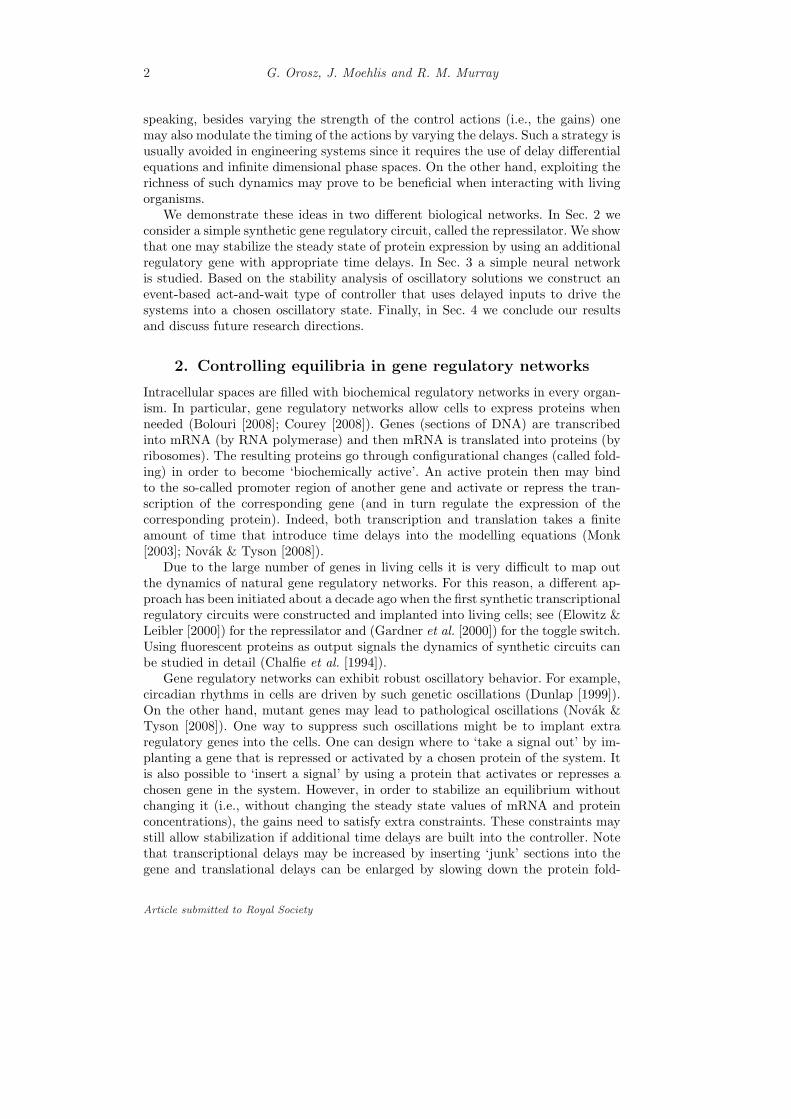
Figure 1. Sketch of the repressilator (subnetwork marked by the dashed frame) with andadditional regulatory gene attached.

ing; see (Ugander [2008]) for more details on delay engineering in transcriptionalregulatory networks.

Here we test these ideas on the repressilator that consists of three genes cou-pled to each other to form a unidirectional ring as depicted by the subnetworkwithin the dashed frame in Fig. 1. Each circle represents a gene and its proteinproduct (Elowitz & Leibler [2000]). This circuit shows robust oscillatory behaviorin wide regions of parameters. It was shown that increasing the transcriptional andtranslational delays between the repressilator elements 1,2,3 leads to more robustoscillations, i.e., they appear in more extended parameter domains and becomemore attractive (Chen & Aihara [2002]; Ugander [2008]). On the other hand, weshow that by attaching an additional element and choosing the corresponding delaysappropriately the oscillations can be suppressed: see the extra regulatory element4 outside the dashed frame in Fig. 1.

The regulated system can be modelled by the delay di"erential equations

mi(t) = !mi(t) + ! f!pi+1(t)

",

pi(t) = !" pi(t) + " mi(t) ,i = 1, 2 ,

m3(t) = !m3(t) + ! f!(1! #)p1(t) + # p4(t)

",

p3(t) = !" p3(t) + " m3(t) ,

m4(t) = !m4(t) + ! f!p2(t! $)

",

p4(t) = !" p4(t) + " m4(t! %) ,

(2.1)

where each gene is repressed through the nonlinear function

f(p) =1

1 + pn+ f0 , (2.2)

that is depicted by the decreasing curve in Fig. 2. Here the dot represents thederivative with respect to time t and mi, pi " 0 are the concentrations of mRNAand protein for the i-th species. For the sake of simplicity, parameters are chosen tobe identical for each gene-protein pair. We assume that the time delays are small



0

pp!

f(p) p/!

1 + f0

f0

Figure 2. Finding the equilibrium value p! of protein concentration. The increasing straightline and the decreasing curve correspond to the left and right sides of the algebraic equation(2.4) where f is given by (2.2).

in the original system (these are set to zero for i = 1, 2, 3), but the extra regulatoryelement contains significant transcriptional and translational delays (denoted by $and % , respectively). The time is measured in units of mRNA degradation time,the protein concentrations are rescaled by the number of proteins needed to half-maximally repress a gene, and the mRNA concentrations are rescaled by the numberof proteins expressed per mRNA molecule in steady state. The rescaled parameters! and " represent the strength of the repression and the protein degradation rate,respectively, and these can be determined from dimensional parameters. In thispaper we consider the ‘leakage constant’ f0 = 10!3 and the Hill coe!cient n = 2,for which oscillations appear in a wide ranges of parameters !,". We recall that! = 215.52, " = 0.2069 were used in (Elowitz & Leibler [2000]) where oscillationswere demonstrated experimentally.

We assume that there is only one binding site at the promoter region of a gene,that is, in case of gene 3 either protein p1 or protein p4 binds but not both; see Fig. 1.More precisely, we assume that p4 binds with probability # # [0, 1] and so p1 bindswith probability (1!#) as expressed in the last term of the equation for m3 in (2.1).Notice that when choosing # = 0 the repressilator with genes 1, 2, 3 is obtained,while for # = 1 another repressilator emerges with genes 2, 3, 4 and time delays $and % . In both of these special cases oscillations occur due to unstable equilibria. Aswill be shown below these oscillations may be suppressed for certain intermediatevalues of # by choosing the delays appropriately. We note that one may modelcompetitive binding by using the nonlinear combination #1f

!p1(t)

"+ #4f

!p4(t)

"

with #1, #4 " 0 instead of f!(1! #)p1(t) + # p4(t)

"in the equation for m3 in (2.1).

The linear stability diagrams obtained in this case are qualitatively similar to thosepresented in this paper. We also remark that there exist genes with multiple bindingsites and one may use the resulting combinatorial features when designing geneticcontrollers (Cox et al. [2007]).

System (2.1) possesses the ‘symmetric’ equilibrium

mi(t) $ pi(t) $ p" , (2.3)



for i = 1, 2, 3, 4 where p" is the unique solution of

p/! = f(p) , (2.4)

as demonstrated in Fig. 2. Note that p" = p"(!, f0, n) and p" is monotonicallyincreasing in !. Also notice that (2.4) is independent of #, $ and % , that is, theextra regulatory gene does not change the equilibrium of the systems. This occurssince the parameters ! and " for the extra element 4 are considered to be identicalto the parameters for the original system 1,2,3. Modulating these parameters (inthe last two equations in (2.1) only) may suppress the oscillations but it destroysthe symmetry and so changes the equilibrium. Contrarily, varying #, $ and % mayallow us to stabilize the equilibrium without altering it.

Let us define the perturbations

ai(t) := mi(t)! p" ,

bi(t) := pi(t)! p" ,(2.5)

and introduce the vector notation

a =#a1 a2 a3 a4

$T,

b =#b1 b2 b3 b4

$T.

(2.6)

Thus, the linearization of (2.1) about (2.3) can be written as%a(t)b(t)

&=

%!I !&A0

"B0 !"I

& %a(t)b(t)

&+

%O !&A!

O O

& %a(t! $)b(t! $)

&+

%O O

"B" O

& %a(t! %)b(t! %)

&,

(2.7)where

A0 =

'

(()

0 1 0 00 0 1 0

1! # 0 0 #0 0 0 0

*

++, , A! =

'

(()

0 0 0 00 0 0 00 0 0 00 1 0 0

*

++, ,

B0 =

'

(()

1 0 0 00 1 0 00 0 1 00 0 0 0

*

++, , B" =

'

(()

0 0 0 00 0 0 00 0 0 00 0 0 1

*

++, ,

(2.8)

I and O denotes the 4% 4 identity and zero matrices, respectively, and

& = f #(p") < 0 . (2.9)

Note that p" = p"(!, f0, n) implies & = &(!, f0, n).Now considering the trial solution a(t) = a e#t, b(t) = b e#t with constant

vectors a, b # R4 and eigenvalues ' # C, the characteristic equation

D(') = det%

(' + 1)I !!&!A0 + A!e!#!

"

!"!B0 + B"e!#"

"(' + ")I

&

= (' + 1)(' + ")-

(' + 1)3(' + ")3 ! (!"&)3!1! # + # e!#(!+")

".= 0(2.10)



is obtained. This equation has infinitely many solutions for the eigenvalues ' incorrespondence to the infinite dimensional phase space of (2.1) and (2.7). The equi-librium (2.3) is asymptotically stable if and only if all eigenvalues lie in the left-halfcomplex plane. When varying the parameters, the equilibrium may lose its sta-bility via Hopf bifurcation if a pair of complex conjugate eigenvalues crosses theimaginary axis. This bifurcation results in periodic oscillations. To determine thestability boundaries we substitute ' = i(, ( # R+ into (2.10), separate the realand imaginary parts and apply some trigonometric identities. The stability curvesin the ($ + %, #) parameter plane are given by

$ + % =1(

/± Arccos

0c21 ! c2

2 ! 2c1 + 1c21 + c2

2 ! 2c1 + 1

1+ (2) + 1)*

2, ) = 0, 1, 2, . . .

# =c21 + c2

2 ! 2c1 + 1!2c1 + 2

,

(2.11)

where

c1 =(" ! (2)

!(" ! (2)2 ! 3(1 + ")2(2

"

(!"&)3,

c2 =(1 + ")(

!3(" ! (2)2 ! (1 + ")2(2

"

(!"&)3,

(2.12)

and the + and ! signs are considered when sin((($+%)) < 0 and sin((($+%)) > 0,respectively.

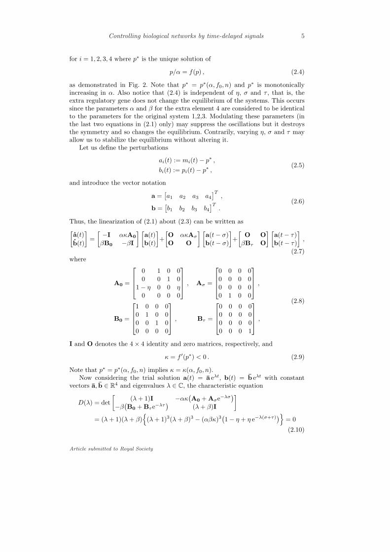
The curves for ) = 0 are plotted in Fig. 3 for di"erent values of ! and ";the original repressilator parameters are used in panel (a). The curves for ) > 0appear for larger delays to the right of the ) = 0 curves and these are out of thewindow. Using infinite dimensional generalizations of the Routh-Hurwitz criteria(Stepan [1989]), one may determine that the steady state is linearly stable in theshaded domain. Notice that when decreasing or increasing ! [panels (a,b,c)] thestable regime does not change significantly, only becoming a bit more extendedcorresponding to the fact that oscillations appear to be most robust for intermediatevalues of ! in the uncontrolled repressilator (Elowitz & Leibler [2000]). On theother hand, the stable domain shrinks and moves closer to the vertical axis whendecreasing " [panels (a,d,e)].

When a stability curve crosses itself a codimension-two Hopf bifurcation oc-curs, i.e., two pairs of complex conjugate eigenvalues cross the imaginary axis thatleads to quasiperiodic oscillations. We remark that such bifurcations occur rarelyin dynamical systems without delay but they are quite typical in delayed systems(Stepan [1989]). Note that the equilibrium may lose its stability via fold bifurca-tion when a real eigenvalue crosses the imaginary axis due to parameter variations.This cannot occur here for $ = % = 0 since & = f #(p") < 0. Consequently, itcannot occur for any $, % > 0 as can be seen by substituting ' = 0 into (2.10).We also remark that incorporating the time delays in the interactions between therepressilator genes 1,2,3 the stability regimes can still be determined, however, thecalculations become more elaborate and so less instructive.

In Fig. 3(b) we marked the points A and B and the corresponding numericalsimulation results are shown in Fig. 4(a) and (b), respectively. In both cases the



! + "

! + " ! + "

! + " ! + "

#

# #

# #

(a)

(b) (c)

(d) (e)

$ = 215.52

$ = 50 $ = 800

$ = 215.52 $ = 215.52

% = 0.2069

% = 0.2069 % = 0.2069

% = 0.1 % = 0.4

A

B

Figure 3. Stability diagrams for the controlled repressilator for di!erent repressionstrengths ! and protein degradation rates ". The equilibrium (2.3) is linearly stable inthe shaded domains. Points A and B in panel (a) correspond the simulations shown inFig. 4(a) and (b), respectively.

same initial conditions are chosen. Recall that the initial conditions for delay dif-ferential equations are functions in the delay interval t # [!max{$, %}, 0], that arechosen to be constant functions here. When the equilibrium is unstable (point A inFig. 3(b) at $+% = 15, # = 0), oscillations arise. The time profiles for the repressila-tor protein concentrations p1, p2, p3 are displayed in the top panel of Fig. 4(a). The



0 50 100 150 2000

40

80

0 50 100 150 2000

40

80

0 50 100 150 2000

40

80

0 50 100 150 2000

40

80

t t

pi pi

p4 p4

(a) (b)

!+"

p1 p2 p3

Figure 4. Demonstrating the action of the genetic controller by numerical simulations. Theprotein concentrations p1, p2, p3 for the repressilator are shown on the top and the proteinconcentration p4 for the extra regulatory gene is displayed at the bottom. Panels (a) and(b) correspond to the points A and B in Fig. 3(a).

system approaches a travelling wave solution where the time profile of the (i+1)-stprotein can be obtained by shifting the time profile of i-th protein by Tp/3 whereTp is the period of oscillations. This pattern corresponds to the Z3 discrete rota-tional symmetry in the system and may also be interpreted as a splay state sincethe concentration of each protein ‘fires’ separately and equidistantly in time. Thetime evolution for the protein concentration p4 is shown in the bottom panel inFig. 4(a). Since # = 0 and p1 and p4 are both driven by p2, the time profiles for p4

can be obtained by shifting the p1 signal with $+% . When the equilibrium is stable(point B in Fig. 3(b) at $ + % = 15, # = 0.25), no oscillations develop as shown inFig. 4(b). This demonstrates that the equilibrium can be stabilized by tuning theaggregated delay $ + % and the binding probability # .

We note that one may find oscillations even for a stable equilibrium when con-sidering certain specific initial conditions. This suggests that the Hopf bifurcationsmay be subcritical. It may be and interesting future research to map out bifurca-tion structure for the arising periodic solutions but that is beyond the scope of thispaper. In the next section however we investigate a time-delayed network where itis essential to study the stability of oscillatory solutions. Such investigations allowus to construct a controller that can stabilize a chosen rhythm.

3. Controlling periodic solutions in neural networks

Oscillations are ubiquitous in neural networks: rhythmic patterns of electric activ-ity are used to represent information about the environment and about the stateof the animal in many di"erent ways (Rabinovich et al. [2006]). However, some ofthese rhythms, for example, full synchrony, may be pathological and lead to macro-scopic tremors like in Parkinson’s disease. (In contrast, in technological systems fullsynchrony is often desired (Olfati-Saber & Murray [2004]).)

One way to avoid these harmful oscillations (without destroying all rhythms)might be to inject weak external current into specific brain areas. For example, wheninjecting di"erent signals at multiple sites, neurons may entrain their rhythms to



1

23

C

Figure 5. Sketch of a network of 3 globally coupled neurons (subnetwork marked by thedashed frame) with a controller attached.

the signal of the nearby electrode and so the overall synchrony can be destroyed(Popovych et al. [2006]). However, this control strategy may force the neural sys-tem into an ‘artificial state’. Instead, one may select a natural rhythm and try tostabilize it. Since neurons communicate with electric signals (called spikes), it takesa considerable amount of time to transmit the signal from one neuron to another.Consequently, time delays appear in the modelling equations. When varying thedelays di"erent stable patterns (e.g., full synchrony, clustering) can emerge (Er-mentrout & Ko [2009]). As will be shown below one may construct a controller thatmimics the delayed interactions of neurons and so drives the system away fromsynchrony into a chosen cluster state.

We demonstrate these ideas in a simple system of three neurons with all-to-allcoupling as depicted inside the dashed frame in Fig. 5. We assume that the voltageof each neuron can be measured and current can be injected into each cell; see thecontroller C outside the dashed frame in Fig. 5. To describe the activity of thesomas we use the Hudgkin-Huxley model which models the cell membrane as asimple electric circuit (Hodgkin & Huxley [1952]). We consider direct electrotoniccouplings (gap junctions) between the neurons and incorporate axonal delays tomodel the time required to transmit the signal along the axons between the neurons.For simplicity, we omit dendritic delays (associated with signal transmission alongdendrites) and synaptic delays (the time needed to release chemicals in synapses);see (Campbell [2007]; Ermentrout & Ko [2009]) for more details on these e"ects.

The time evolution of the controlled system is given by the delay di"erential



equations

Vi(t) =1C

0I ! gNam

3i (t)hi(t)

!Vi(t)! VNa

"! gKn4

i (t)!Vi(t)! VK

"! gL

!Vi(t)! VL

"

+ +33

i=1,i $=j

!Vj(t! ,)! Vi(t)

"+ - ui(t)

1,

mi(t) = !m

!Vi(t)

"!1!mi(t)

"! "m

!Vi(t)

"mi(t) ,

hi(t) = !h

!Vi(t)

"!1! hi(t)

"! "h

!Vi(t)

"hi(t) ,

ni(t) = !n

!Vi(t)

"!1! ni(t)

"! "n

!Vi(t)

"ni(t) , i = 1, 2, 3,

(3.1)

where the dot represents the derivative with respect to time t (measured in ms), Vi

is the voltage of the i-th neuron (measured in mV), and the dimensionless quantitiesmi, hi, ni # [0, 1] (called gating variables) characterize the ‘openness’ of the sodiumand potassium ion channels embedded in the cell membrane. The conductances gNa,gK, gL and the reference voltages VNa, VK, VL for the sodium channels, potassiumchannels and the so-called ‘leakage current’ are given together with the membranecapacitance C and the driving current I in Appendix A by (A 1).

The term proportional to + describes the electrotonic coupling between neurons.The conductance + represents the coupling strength and , is the transmission delaydescribed above. The term proportional to - represents the control signal. Thecoe!cient - is the magnitude of the injected current and ui(t) describes the timevariation of the input such that it can take the discrete values 0, 1, 2. We assumethat both the coupling and the input are weak, that is, +, - & 1, and that they arein the same order of magnitude, i.e., - = O(|V |+). For the parameters consideredwe have |V | ' 100 and here we set - = 250 +. The equations for mi, hi, ni arebased on measurements and the nonlinear functions !m(V ), !h(V ), !n(V ), "m(V ),"h(V ), "n(V ) are given in Appendix A by (A2).

First, we describe the dynamics without inputs (- = 0) when varying the cou-pling strength + and the coupling delay ,. For + = 0 the neurons are uncoupledand spike periodically (with period Tp ' 10.43). For small + > 0 the qualitativeshape of oscillations do not change but di"erent cluster states can arise through theelectronic interactions. In particular, three di"erent patterns may exist: full syn-chrony (when all three neurons spike together); splay state (when no neurons spiketogether); and 1:2 state (when only two neurons spike together). These patternscorrespond to the S3 permutational symmetry in the system (interchangeability ofneurons for - = 0) and these may be found by numerical simulation. Fig. 6 showsthe simulation results for parameters , = 5.5, + = 0.03 where all cluster states arestable: it depends on the initial conditions which state emerges. (The initial con-ditions are again chosen to be constant functions in the delay interval t # [!,, 0].)Notice that spikes are evenly spaced in the splay state in correspondence to the S3

permutational symmetry. In the 1:2 state the phase di"erence between the pair andthe singleton depends on the parameters and generally spikes are not evenly spaced.We remark that there are always two di"erent splay states (distinguished by theorder of spikes) and three di"erent 1:2 states (distinguished by which oscillator isthe singleton). For more details on clustering in globally coupled neural systems see(Brown et al. [2003]; Coombes [2008]; Orosz et al. [2009b]).



0 10 20 30 40 50 60−80

0

50

0 10 20 30 40 50 60−80

0

50

0 10 20 30 40 50 60−80

0

50

t !

Vi

"

Vi

"

Vi

"

(a) (b)sync sync

splay splay

1:2 1:2

V1 V3 V2

V1 V2,3

pd

f

f

ns ns ns

ns

ns

f f

Figure 6. Di!erent neural clusterings are shown in panel (a) and the related (#, $) stabilitycharts are displayed in panel (b). The shaded domains indicate stability and f, pd and nsdenote fold, period doubling, and Neimark-Sacker bifurcations. The !-s at # = 5.5, $ = 0.3in panel (b) correspond to the parameters used in panel (a).

The di"erent cluster states correspond to periodic orbits in phase space and oneneeds to use Floquet theory to determine their stability. In particular, the eigenval-ues of the solution operator of (3.1) at Tp, the so-called Floquet multipliers, need tobe calculated. A periodic motion is stable if all the infinitely many multipliers arelocated inside the unit circle in the complex plane. When varying the parametersstability losses may occur via fold bifurcation (when a real multiplier crosses theunit circle at +1), via period doubling bifurcation (when a real multiplier crossesthe unit circle at !1), and via Neimark-Sacker bifurcation (when a pair of complexconjugate multipliers crosses the unit circle). Di"erent periodic and quasiperiodicoscillations may arise through these bifurcations that are not discussed here indetail.

It is not possible to determine the stability boundaries in parameter space ana-lytically but there exist numerical methods to perform this task. We use numericalcontinuation techniques, in particular the package DDE-Biftool, that allow us tofollow branches of oscillatory solutions (both stable and unstable) as a function ofparameters and detect the above bifurcation (Roose & Szalai [2007]). In order todetermine the stability, the solution operator is discretized and represented by alarge matrix whose eigenvalues approximate the Floquet multipliers. We remarkthat for large numbers of neurons one may apply semi-analytical methods to de-termine the stability for specific cluster states (e.g., the synchronized state and thesplay state); see (Coombes [2008]).

We varied the delay parameter , and detected the above bifurcations for severaldi"erent values of + and the results are shown in the stability charts in Fig. 6(b).Shading indicates stability, the fold, period doubling and Neimark-Sacker bifur-cations are denoted by f, pd and ns, respectively, and the %-s correspond to theparameter values , = 5.5, + = 0.03 used in Fig. 6(a). The ‘sharp edges’ alongthe stability boundaries correspond to codimension-two bifurcations, for example,the synchronized state undergoes a fold-period doubling bifurcation and the splaystate undergoes a double Neimark-Sacker bifurcation. The dynamics is potentiallycomplex around such points. Furthermore, in certain regimes multiple unstable so-



0 5 10 15−80

0

50

0 5 10 15

0 5 10 15

Vi

u1

u2

u3

t

V2 V1 V3

t0 t1 t2 t3

tw ta

Figure 7. The event-based act-and-wait control algorithm: after a neuron spikes the con-troller ‘waits’ tw time and then ‘acts’ for ta time by injecting constant inputs to the othertwo neurons; see (3.2). Notice that ta " tw. From top to bottom: the voltage oscillations;the recorded spike times; the input signals.

lutions coexist with the stable solutions and the stable manifolds of the unstablesolutions separate the regions of attractions of the stable solutions in state space.Unfolding these complexities is beyond the scope of this paper.

By studying the stability diagrams one may observe the qualitative changes ofemergent dynamics as the time delay increases. For small delays (including zerodelay) only the synchronous state is stable. This is followed by di"erent domainsof mono-, bi- and tristability. That is, by varying the time delay di"erent clusterstates may be realized.

Indeed, it is not possible to tune the natural delays in the system. However, thecontroller may inject external signals that mimic the e"ects of delayed coupling.To this end we construct an event-based act-and-wait controller (Danzl & Moehlis[2007]; Insperger [2006]) as follows. We record the event when a neuron spikes andafter time tw a constant signal of length ta is injected to the other two neurons. Thetime intervals tw and ta are called the ‘wait time’ and the ‘act time’, respectively.Considering the initial condition ui(0) = 0, i = 1, 2, 3, the control rules can beformalized as follows.

If neuron i spikes at t = t0 then

u+j (t0 + tw) = u!j (t0 + tw) + 1

u+j (t0 + tw + ta) = u!j (t0 + tw + ta)! 1

for all j (= i.

(3.2)

This algorithm is demonstrated in Fig. 7. Recall that ui(t) can only take the discretevalues 0, 1, 2 such that ui(t) = 2 occurs if at least two neurons spiked within a timeinterval of ta. In order to obtain ‘spiky’ inputs we consider ta & tw. In particular,we fix the act time at ta = 0.5 and vary the wait time tw.

We define a scalar observable, called the order parameter, to quantify the emer-gent state of the system:

R =13

4444ei 2$

t1!t0t3!t0 + ei 2$

t2!t0t3!t0 + ei 2$

4444 . (3.3)



0 50 100 150 200−80

0 50

0 50 100 150 200

0 50 100 150 200

0 50 100 150 2000

0.5

1

Vi

u1

u2

u3

R

t

Figure 8. Driving the system from full synchrony to a splay state with the controller for# = 0, $ = 0.06 and tw = 6.0. From top to bottom: the voltage oscillations; the recordedspike times; the input signals; the order parameter (3.3).

This represents the phase relation of the last four spikes arrived at t0 ) t1 )t2 ) t3, such that the spikes at t0 and t3 were produced by the same neuronwhile the spikes at t1 and t2 were produced by the other two neurons; see Fig .7.This quantity has to be updated when a new spike arrives at t4 according to theupdate rule t0 * t1, t1 * t2, t2 * t3, t3 * t4. In fact, R is an ‘event-basedversion’ of the order parameter used in phase oscillator networks where the phaseinformation is continuously available (Strogatz [2000]). Notice that R = 1 for thefully synchronous state and R = 0 for the splay state (with evenly spaced spikes).For the 1:2 state (with general phase di"erence between the singleton and the pair)we have 1/3 ) R < 1 such that the minimum R = 1/3 is reached when the spikesare evenly spaced.

In Fig. 8 the controller’s action is shown for parameters , = 0, + = 0.06. One mayobserve that without inputs (t ! 50) the system approaches the fully synchronousstate since that is the only stable state for these parameters; see Fig. 6(b). Aftereach neuron has spiked five times the controller is switched on using tw = 6.0.(Notice that for , = 6.0, + = 0.06 the synchronous state is unstable in Fig. 6(b)).The controller drives the system away from the fully synchronous state into a splaystate as shown in the top two panels in Fig. 8. The changes in the spatiotemporalpattern of inputs and the time evolution of the order parameter R (that goes from1 to 0) are displayed it the bottom panels.

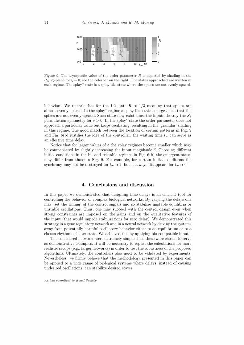
In order to test the robustness of the proposed algorithm we vary the waittime tw and the coupling strength + (for zero coupling delay , = 0) and read theasymptotic value of the order parameter (taken at t = 1000). The shading of the(tw, +)-plane in Fig. 9 represents the value of R such that white corresponds to R = 0(splay state) while the darkest tone corresponds to R = 1 (synchronized state).Notice the well pronounced boundaries between regions of qualitatively di"erent



0 2 4 6 8 10 120.01

0.05

0.09

!

tw

R

0

13

23

1

sync

spla

y

sync 1:2

spla

y

spla

y!

sync

Figure 9. The asymptotic value of the order parameter R is depicted by shading in the(tw, $)-plane for # = 0; see the colorbar on the right. The states approached are written ineach regime. The splay* state is a splay-like state where the spikes are not evenly spaced.

behaviors. We remark that for the 1:2 state R ' 1/3 meaning that spikes arealmost evenly spaced. In the splay" regime a splay-like state emerges such that thespikes are not evenly spaced. Such state may exist since the inputs destroy the S3

permutation symmetry for - > 0. In the splay" state the order parameter does notapproach a particular value but keeps oscillating, resulting in the ‘granular’ shadingin this regime. The good match between the location of certain patterns in Fig. 9and Fig. 6(b) justifies the idea of the controller: the waiting time tw can serve asan e"ective time delay.

Notice that for larger values of + the splay regimes become smaller which maybe compensated by slightly increasing the input magnitude -. Choosing di"erentinitial conditions in the bi- and tristable regimes in Fig. 6(b) the emergent statesmay di"er from those in Fig. 9. For example, for certain initial conditions thesynchrony may not be destroyed for tw ' 2, but it always disappears for tw ' 6.

4. Conclusions and discussion

In this paper we demonstrated that designing time delays is an e!cient tool forcontrolling the behavior of complex biological networks. By varying the delays onemay ‘set the timing’ of the control signals and so stabilize unstable equilibria orunstable oscillations. Thus, one may succeed with the control design even whenstrong constraints are imposed on the gains and on the qualitative features ofthe input (that would impede stabilizations for zero delay). We demonstrated thisstrategy in a gene regulatory network and in a neural network by driving the systemsaway from potentially harmful oscillatory behavior either to an equilibrium or to achosen rhythmic cluster state. We achieved this by applying bio-compatible inputs.

The considered networks were extremely simple since these were chosen to serveas demonstrative examples. It will be necessary to repeat the calculations for morerealistic setups (e.g., larger networks) in order to test the robustness of the proposedalgorithms. Ultimately, the controllers also need to be validated by experiments.Nevertheless, we firmly believe that the methodology presented in this paper canbe applied to a wide range of biological systems where delays, instead of causingundesired oscillations, can stabilize desired states.



Appendix A. Parameters for the Hodgkin-Huxley model

Here we define the parameters

gNa = 120 [mS/cm2] , VNa = 50 [mV] ,gK = 36 [mS/cm2] , VK = !77 [mV] ,gL = 0.3 [mS/cm2] , VL = !54.4 [mV] ,I = 20 [µA/cm2] , C = 1 [µF/cm2] ,

(A 1)

and the functions

!m(V ) = 0.1 (V +40)

1!e!V +40

10, "m(V ) = 4 e!

V +6518 ,

!h(V ) = 0.07 e!V +65

20 , "h(V ) = 1

1+e!V +35

10,

!n(V ) = 0.01 (V +55)

1!e!V +55

10, "n(V ) = 0.125 e!

V +6580 .

(A 2)

used in the Hodgkin-Huxley model (3.1).

References

Astrom, K. J. & Murray, R. M. 2008 Feedback systems: An introduction for scien-tists and engineers. Princeton University Press.

Bolouri, H. 2008 Computational modeling of gene regulatory networks – a primer.Imperial College Press.

Brown, E., Holmes, P. & Moehlis, J. 2003 Globally coupled oscillator networks. InPerspectives and problems in nonlinear science: A celebratory volume in honor ofLarry Sirovich (eds E. Kaplan, J. E. Marsden & K. R. Sreenivasan), pp. 183–215.Springer.

Campbell, S. A. 2007 Time delays in neural systems. In Handbook of brain connec-tivity (eds V. K. Jirsa & A. R. McIntosh), Understanding Complex Systems, pp.65–90. Springer.

Chalfie, M., Tu, Y., Euskirchen, G., Ward, W. W. & Prasher, D. C. 1994 Greenfluorescent protein as a marker of gene-expression. Science, 263(5148), 802–805.

Chen, L. & Aihara, K. 2002 Stability of genetic regulatory networks with timedelay. IEEE Transactions on circuits and systems I: Fundamental Theory andApplications, 49(5), 602–608.

Coombes, S. 2008 Neuronal network with gap junctions: a study of piecewise linearplanar neuron models. SIAM Journal on Applied Dynamical Systems, 7(3), 1101–1129.

Coombes, S. & Laing, C. 2009 Delays in activity-based neural networks. Philosoph-ical Transactions of The Royal Society A, 367(1891), 1117–1129.

Courey, A. J. 2008 Mechanisms in transcriptional regulation. Blackwell Publishing.

Cox, R. S., Surette, M. G. & Elowitz, M. B. 2007 Programming gene expressionwith combinatorial promoters. Molecular Systems Biology, 3(145), 1–11.



Danzl, P. & Moehlis, J. 2007 Event-based feedback control of nonlinear oscillatorsusing phase response curves. In Proceedings of the 46th IEEE conference ondecision and control, pp. 5806–5811.

Dombovari, Z., Wilson, R. E. & Stepan, G. 2008 Estimates of the bistable regionin metal cutting. Proceedings of the Royal Society A, 464(2100), 3255–3271.

Dunlap, J. C. 1999 Molecular bases for circadian clocks. Cell, 96(2), 271–290.

Elowitz, M. B. & Leibler, S. 2000 A synthetic oscillatory network of transcriptionalregulators. Nature, 403(6767), 335–338.

Ermentrout, B. & Ko, T.-W. 2009 Delays and weakly coupled neuronal oscillators.Philosophical Transactions of The Royal Society A, 367(1891), 1097–1115.

Gardner, T. S., Cantor, C. R. & Collins, J. J. 2000 Construction of a genetic toggleswitch in Escherichia coli. Nature, 403(6767), 339–342.

Hodgkin, A. L. & Huxley, A. F. 1952 A quantitative description of membranecurrent and its application to conduction and excitation in nerve. Journal ofPhysiology, 117(4), 500–544.

Insperger, T. 2006 Act-and-wait concept for continuous-time control systems withfeedback delay. IEEE Transactions on Control Systems Technology, 14(5), 974–977.

Kirst, C., Geisel, T. & Timme, M. 2009 Sequential desynchronization in networksof spiking neurons. Physical Review Letters, 102(6), 068 101.

Mascolo, S. 1999 Congestion control in high-speed communication networks usingthe Smith principle. Automatica, 35(12), 1921–1935.

Monk, N. A. M. 2003 Oscillatory expression of Hes1, p53, and NF-&B driven bytranscriptional time delays. Current Biology, 13(16), 1409–1413.

Novak, B. & Tyson, J. J. 2008 Design principles of biochemical oscillators. NatureReviews Molecular Cell Biology, 9(12), 981–991.

Olfati-Saber, R. & Murray, R. M. 2004 Consensus problems in networks of agentswith switching topology and time-delays. IEEE Transactions on Automatic Con-trol, 49(9), 1520–1533.

Orosz, G., Ashwin, P. & Townley, S. 2009a Learning of spatio-temporal codes in acoupled oscillator system. IEEE Transactions on Neural Networks, 20(7), 1135–1147.

Orosz, G., Moehlis, J. & Ashwin, P. 2009b Designing the dynamics of globallycoupled oscillators. Progress of Theoretical Physics, 122(3).

Popovych, O., Hauptmann, C. & Tass, P. A. 2006 Control of neuronal synchronyby nonlinear delayed feedback. Biological Cybernetics, 95(1), 69–85.

Rabinovich, M. I., Varona, P., Selverston, A. I. & Abarbanel, H. D. I. 2006 Dynam-ical principles in neuroscience. Reviews of Modern Physics, 78(4), 1213–1265.



Roose, D. & Szalai, R. 2007 Continuation and bifurcation analysis of delay dif-ferential equations. In Numerical continuation methods for dynamical systems(eds B. Krauskopf, H. M. Osinga & J. Galan-Vioque), Understanding ComplexSystems, pp. 359–399. Springer.

Sarpeshkar, R., Wattanapanitch, W., Arfin, S. K., Rapoport, B. I., Mandal, S.,Baker, M. W., Fee, M. S., Musallam, S. & Andersen, R. A. 2008 Low-powercircuits for brain-machine interfaces. IEEE Transactions on Biomedical Circuitsand Systems, 2(3), 173–183.

Stepan, G. 1989 Retarded dynamical systems: Stability and characteristic functions,vol. 210 of Pitman Research Notes in Mathematics. Longman.

Stepan, G. 2001 Vibrations of machines subjected to digital force control. Interna-tional Journal of Solids and Structures, 38(10-13), 2149–2159.

Stricker, J., Cookson, S., Bennett, M. R., Mather, W. H., Tsimring, L. S. & Hasty,J. 2008 A fast, robust and tunable synthetic gene oscillator. Nature, 456(7221),516–U39.

Strogatz, S. H. 2000 From Kuramoto to Crawford: exploring the onset of synchro-nization in populations of coupled oscillators. Physica D, 143(1-4), 1–20.

Ugander, J. 2008 Delay-dependent stability of genetic regulatory networks.Master’s thesis, Department of Automatic Control, Lund University, Sweden.https://www.control.lth.se/database/publications/article.pike?artkey=5819.


controlling biological networks by time-delayed signalsmurray/preprints/omm09-ptrs-a_s.pdf · ploit...

Documents