control systems engineering - rpicats-fs.rpi.edu/~wenj/ecse444f05/nov04matlabsimulinkpid.pdf ·...
TRANSCRIPT
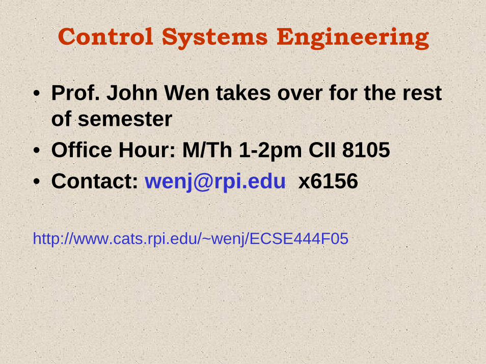
Control Systems Engineering
• Prof. John Wen takes over for the rest of semester
• Office Hour: M/Th 1-2pm CII 8105• Contact: [email protected] x6156
http://www.cats.rpi.edu/~wenj/ECSE444F05

Remainder of Semester
Date Topic11/4 MATLAB & Simulink, PID control and gain tuning11/8 Design project description11/11 Introduction to the state space method11/15 Full state feedback and pole placement11/18 State estimator11/22 Tracking control11/29 Digital implementation12/2 Design example12/6 Design example12/9 Review

• Design Project: 25%, group of 2, design report, due on 12/9.
• Final exam: 25% (12/14, 6:30-9:30)• Homework: 25% total
Your Grade
• MATLAB & Simulink• PID Control and Gain Tuning
Today
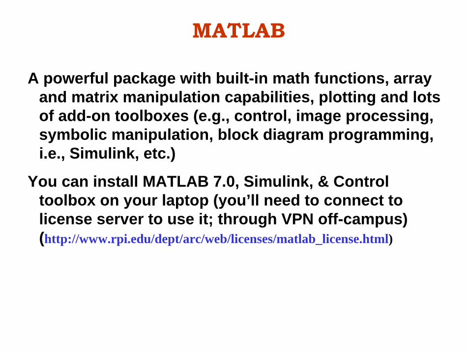
MATLAB
A powerful package with built-in math functions, array and matrix manipulation capabilities, plotting and lots of add-on toolboxes (e.g., control, image processing, symbolic manipulation, block diagram programming, i.e., Simulink, etc.)
You can install MATLAB 7.0, Simulink, & Control toolbox on your laptop (you’ll need to connect to license server to use it; through VPN off-campus) (http://www.rpi.edu/dept/arc/web/licenses/matlab_license.html)

An interpretive environment, may use scripts
• Vectors: theta=[theta_1;theta_2];• Matrices: M=[M11 M12; M21 M22];• Polynomials: p=[a3 a2 a1 a0];• Transfer functions: G=tf(num,den);• Linear simulation:
• step response: step(G);• impulse response: impulse(G);• general response: y=lsim(G,u,t);
MATLAB (Cont.)

• Plotting: plot(t,x1,t,x2);xlabel(‘time (sec)’);ylabel(‘theta(deg)’); title(‘theta(t)’); legend(‘\theta_1’,’\theta_2’);
• Printing (to printer or file)print -f -d<device type> <file name>
• Using m-files in MATLABuse any editor (or MATLAB built-in editor, just type in edit)function f=func(t,x) ...
• Getting help in MATLAB: help <function name> or just help
Always label axes, include units, and include legends in your plots.
on-line tutorial: http://www.engin.umich.edu/group/ctm/
MATLAB (Cont.)

Description of LTI Systems
Input/Output (differential equation)
Frequency Domain State Space
What does LTI mean?
Input output
state

Description of LTI Systems
Input/Output (differential equation)
Frequency Domain State Space
( )dM D Kθ θ θ θ τ+ + − =
2 1
( )
( ) ( ) ( )G s
s s M Ds K sθ τ−Δ = + +
[ ]
1 1 1
0 0
0 0A B
DC
Ix x
M K M D M
y I x
τ
τ
− − −
⎡ ⎤ ⎡ ⎤= +⎢ ⎥ ⎢ ⎥− −⎣ ⎦ ⎣ ⎦
= +
1
2
dxx
xθ θθ−⎡ ⎤ ⎡ ⎤
= =⎢ ⎥ ⎢ ⎥⎣ ⎦⎣ ⎦
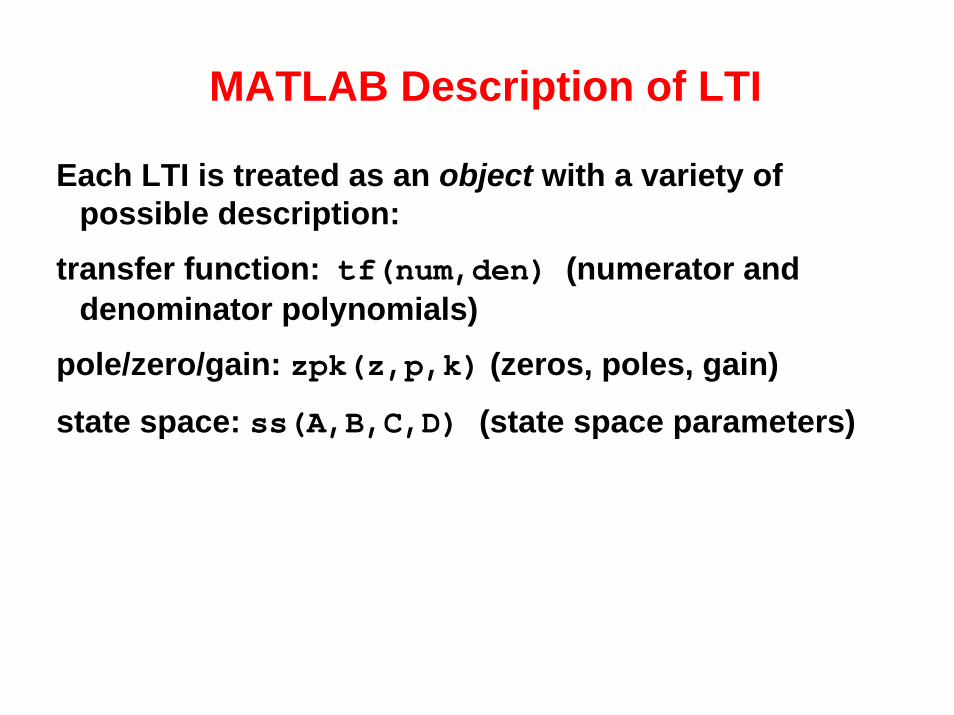
MATLAB Description of LTI
Each LTI is treated as an object with a variety of possible description:
transfer function: tf(num,den) (numerator and denominator polynomials)
pole/zero/gain: zpk(z,p,k) (zeros, poles, gain)
state space: ss(A,B,C,D) (state space parameters)
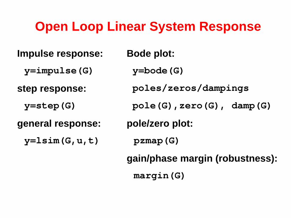
Open Loop Linear System Response
Impulse response:y=impulse(G)
step response:y=step(G)
general response:y=lsim(G,u,t)
Bode plot:y=bode(G)
poles/zeros/dampings
pole(G),zero(G), damp(G)
pole/zero plot:pzmap(G)
gain/phase margin (robustness):margin(G)

Incorporation of Control
Interconnection of LTI systems:
τ θG
H
KFr
-
+
Gcl = feedback(G*K,H)*F

Simulink
Instead of command line entries, it may be easier to use a block diagram programming tool:
LTI block(s-1)
s(s+1)Zero-Pole
1
s+1Transfer Fcn1
x' = Ax+Bu y = Cx+Du
State-Space
s +.1s+10210
Transfer Fcn
y
To Workspace
Scope
1
Constant
s +.1s+10210
Transfer Fcn
y
To Workspace
Scope
PID
PID Controller(with Approximate
Derivative)
1
Constant

Effect of Sampling
Most control systems these days are digital in nature so sampling is inherent (through A/D for sensor, which contains a sampler, and D/A for actuators, which contains a zero-order-hold).
To analyze the effect of sampling, we can find the equivalent discrete time system:
Gd = c2d(G,ts);%ts=sampling period (sec)
Gd is also an LTI object and the commands for LTI may be applied.

Adding Sampling to Simulink Diagram
To add sampling to your continuous time simulation, just add a zero-order-hold block (in the discrete time system library) to the input, then set the sampling time.
Zero-OrderHold
s +.1s+10210
Transfer Fcn
y
To Workspace
Scope
PID
PID Controller(with Approximate
Derivative)
1
Constant
MATLAB and Simulink
MATLAB and Simulink are the de facto industry standard, you should try to master them.
You’ll also need to use MATLAB and Simulink in your design project.

Quick Review of Control DesignWhy feedback?
• Stability (closed loop poles in LHP)• Performance (rise time, overshoot, settling
time)• Steady state (steady state error)• Robustness (gain/phase margin)• Disturbance rejection (loop shaping)• Tracking (loop shaping / feedforward)

Example: 1st Order System
• First order system: One pole only• Target output: yd
• Proportional control: u = - kp ( y-yd )
yu1
d 1 2y u u du
= − −
s1
du y
Is this system stable?
u2

Example: 1st Order System
duy −=
s1
du y
pkdy
pd
p
p
ksdy
ksk
y+
−+
=
×
• Stable if kp >0• No overshoot, faster rise
time, smaller settling time if kp large
• Steady state error:
pss
pd
p
kde
ksdy
ksse
−=
+−
+−=
×
open loop
pk20dB/decade roll-off
-45o
-90o
0dB
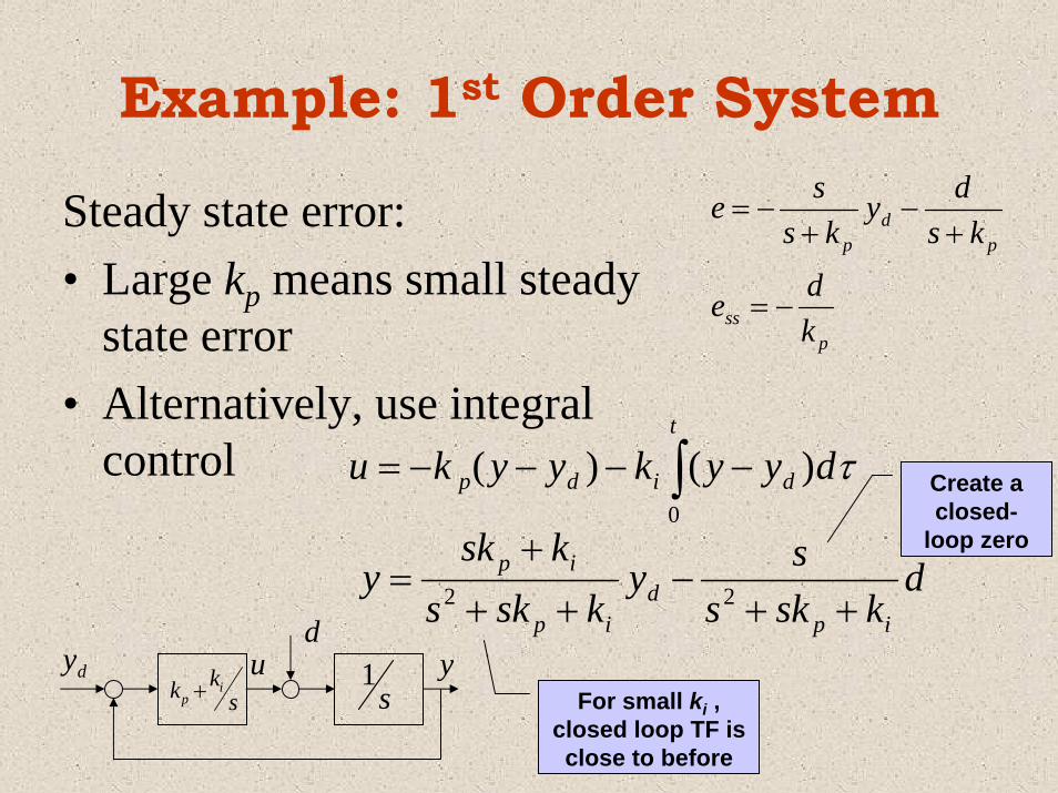
Example: 1st Order System
Steady state error:• Large kp means small steady
state error• Alternatively, use integral
control
pss
pd
p
kde
ksdy
ksse
−=
+−
+−=
∫ −−−−=t
didp dyykyyku0
)()( τ
dksks
syksks
ksky
ipd
ip
ip
++−
++
+= 22
s1
du y
skk i
p +dy
Create a closed-
loop zero
For small ki , closed loop TF is close to before

Example: 1st Order System
Integral control• CL system is 2nd order• Choose kp ki to achieve desired
transient response• Steady state error due to step
disturbance is zero!
0
22
2
=
++−
++−
=
ss
ipd
ip
e
dksks
syksks
se
s1
du y
skk i
p +dy

Example: 2nd Order SystemOrientation control of Satellite:
Proportional feedback duy +=
21
s
du y
pkdy
pd
p
p
ksdy
ksk
y+
++
= 22
• Closed loop poles at +/- kp j• Marginally stable if kp >0
× open loop×
×
)( dp yyku −−=

Example: 2nd Order SystemProportional-derivative feedback duy +=
21
s
du y
skk dp +dy
pdd
pd
pd
ksksdy
ksksksk
y++
+++
+= 22
• Stable if kp >0 and kd >0• Choose gains to achieve
desired transient response• Steady state error:
ykyyku ddp
× open loop×
−−−= )(
dp kk /−p
ss
pdd
pd
kde
ksksdy
ksksse
=
+++
++−
= 22
2

Example: 2nd Order SystemProportional-integral-derivative
(PID) controlduy +=
21
s
du y
skskk i
dp ++dy
ipdd
ipd
pd
kskskssdy
kskskssksk
y+++
++++
+= 2323
2• Stable if kp >0 and kd >0 and
ki>0 sufficiently small• Choose gains to achieve
desired transient response• Zero steady state error for
step disturbance × open loop×
∫ −−−−−=t
diddp dyykykyyku0
)()( τ
dp kk /−×

Other Issues• Tracking control: Replace the step yd by the
desired time varying yd (t) – keep closed loop transfer function around 1 (0dB, 0 phase) in the spectrum of yd (t).
• What if the system is not second order? – Use the dominant second order system (two poles
closest to the -axis)– Check stability / performance / steady state error
on the high order system
ωj
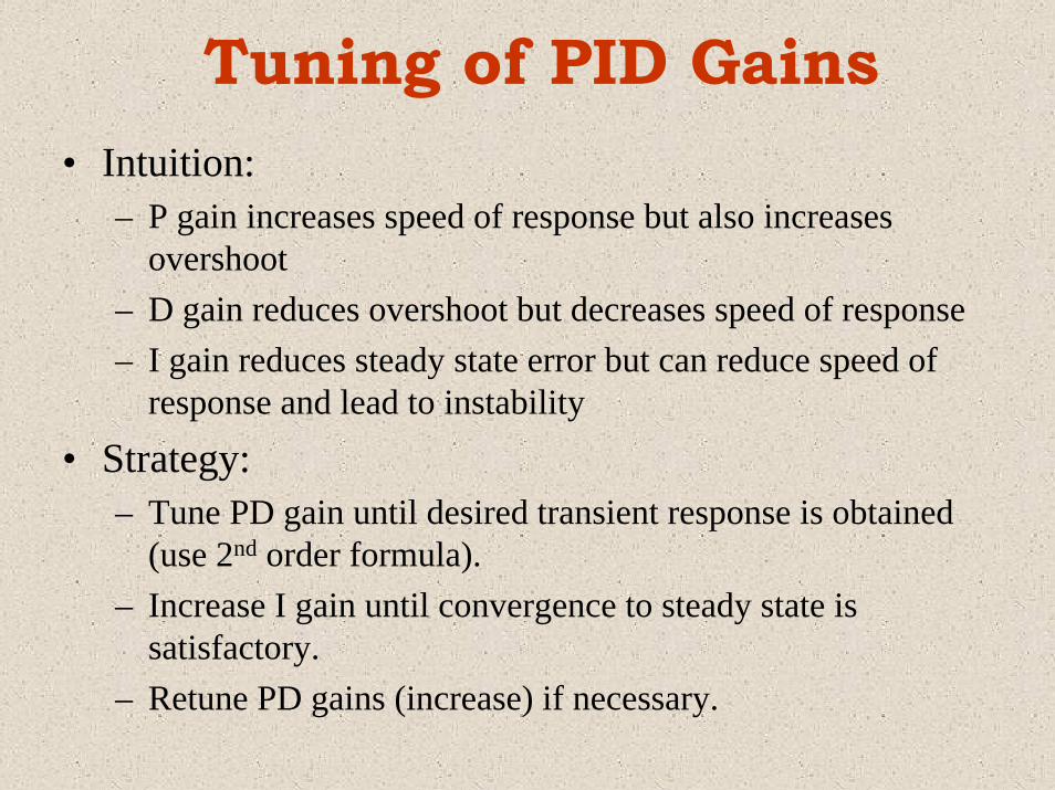
Tuning of PID Gains• Intuition:
– P gain increases speed of response but also increases overshoot
– D gain reduces overshoot but decreases speed of response– I gain reduces steady state error but can reduce speed of
response and lead to instability
• Strategy: – Tune PD gain until desired transient response is obtained
(use 2nd order formula). – Increase I gain until convergence to steady state is
satisfactory. – Retune PD gains (increase) if necessary.

Ziegler-Nichols Tuning Guide• Approximate the system as a first order
system with delay (motivated by process control) slope = R
delay = LLT
LTRLK
sTsTKsD
D
I
DI
5.02
/2.1)/11()(
===
++=
• Use proportional feedback to drive the system to the boundary of instability (ultimate gain: Ku ultimate period: Pu)
uD
uI
u
PT
PTKK
815.06.0
=
==

Computational Approach• Parameterize PID controller as
with K and a chosen within a range (based on bandwidth, sampling, and saturation consideration).
• Step through K and a to minimize some combination of performance measures (e.g., overshoot, settling time, rise time, etc.).
• MATLAB is a great tool for this approach.
2( )( )cs aG s K
s+
=

Digital Control
• Sample data implementation: we need to approximate the derivative and integral terms
• Derivative term: backward difference
∫ −−−−−=t
diddp dyykykyyku0
)()( τ
ytzw
tyyw
yw
s
s
kkk
⎥⎦⎤
⎢⎣⎡ −≅
−≅
=
−
−
)1( 1
1• Integral term: cumulative sum
yztw
tyww
yw
s
skkk
⎥⎦⎤
⎢⎣⎡
−≅
+≅
=
−
−
∫
)1( 1
1
• Stability: closed loop poles within unit circle

Digital Control• Stability: closed loop poles within unit circle• Rule of thumb: 3 to 10 times faster than closed
loop bandwidth – With a specified sampling rate, poles cannot be too fast
(i.e., gains cannot be too high)• First order system example:
nω
)(1 dkpskk yyktyy −−=+
sp
ps
ps
tk
kt
ktz
/1:stabilityfor Condition
)(1:poles loop Closed
0)(1-equation sticcharacteri loop Closed
<
−
=−
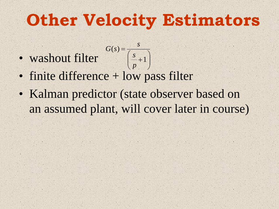
Other Velocity Estimators
• washout filter• finite difference + low pass filter• Kalman predictor (state observer based on
an assumed plant, will cover later in course)
⎟⎟⎠
⎞⎜⎜⎝
⎛+
=1
)(
ps
ssG