AUTOMATED JUGGLER by

John Carpenter Shannon Jordan Daniel Grover

ECSE-4962 Control Systems Design

Final Project Report April 28, 2004

Rensselaer Polytechnic Institute

ii

ABSTRACT

The Automated Juggler is a control system which will toss a ball into the air, using its tilt axis, and subsequently catch it, by rotating its pan axis if needed. As the design is significantly physics based, this report will discuss the basic physics models that were derived during the design process. A primary concern when designing the system was the maximum angular velocity and deceleration it was able to obtain. These criteria were the limiting factors on both whether the system would be able to perform its task, and also how well it would be able to perform its task. The report will also discuss the abnormal effect of viscous and Coulomb friction, and how this was accounted for in the system. Lastly, the system has to be able to follow a control signal well, and have limited error overall. With all of these tasks functioning as planned, the Automated Juggler is a success.

iii

TABLE OF CONTENTS 1. INTRODUCTION ...................................................................................................................... 1 2. PROFESSIONAL AND SOCIETAL CONSIDERATION........................................................ 2 3. DESIGN PROCEDURE ............................................................................................................. 3

3.1 Modeling ............................................................................................................................... 3 Non-linear Model:................................................................................................................... 3 Linear Model:.......................................................................................................................... 3

3.2 Model Validation .................................................................................................................. 3 3.3 Control Design and Tuning................................................................................................... 4 3.4 Design Iteration..................................................................................................................... 4 3.5 Performance Verification...................................................................................................... 4

4. DESIGN DETAILS .................................................................................................................... 5 4.1 Initial Calculations ................................................................................................................ 5 4.2 Friction Testing..................................................................................................................... 5 4.3 Trajectory Design and Analysis.......................................................................................... 11 4.5 Control Signal ..................................................................................................................... 19 4.5 Modeling ............................................................................................................................. 21

Non-linear Model:................................................................................................................. 21 Linear Model:........................................................................................................................ 23

4.6 Control Design .................................................................................................................... 23 4.7 Error Analysis ..................................................................................................................... 29 4.8 Modifications of the Mechanical System ........................................................................... 30

5. DESIGN VERIFICATION....................................................................................................... 31 5.1 Model Verification.............................................................................................................. 31 5.2 System Performance ........................................................................................................... 35

6. COSTS AND SCHEDULE....................................................................................................... 40 6.1 Costs.................................................................................................................................... 40 6.2 Schedule.............................................................................................................................. 41

7. CONCLUSIONS....................................................................................................................... 42 8. REFERENCES ......................................................................................................................... 43 APPENDIX A: NONLINEAR MODEL INCORPORATING NONLINEAR FRICTION......... 44 APPENDIX B: PHYSICAL SYSTEM CONTROL, PAN AND TILT ....................................... 45 APPENDIX C: MOTOR SPECIFICATION SHEET................................................................... 46 APPENDIX D: MASS AND INERTIA SCRIPTS ...................................................................... 47 APPENDIX E: FRICTION TESTING SCRIPTS ........................................................................ 50 APPENDIX F: TRAJECTORY ANALYSIS ............................................................................... 53 APPENDIX G: CONTROL SIGNAL .......................................................................................... 56 APPENDIX H: CONTROLLER DESIGN................................................................................... 58 APPENDIX I: ERROR CALCULATIONS ................................................................................. 60 APPENDIX J: CONTRIBUTION OF TEAM MEMBERS ......................................................... 61

iv

LIST OF FIGURES Fig. 1. Friction ID Testing in Simulink........................................................................................... 6 Fig. 2. Example of Velocity and Filtered Velocity Curves at 0.69 V............................................. 6 Fig. 3: Last 100 Samples of Tilt Velocity Curve ............................................................................ 7 Fig. 4. Friction ID Testing for Tilt Motor....................................................................................... 8 Fig. 5. Friction ID Testing for Pan Motor....................................................................................... 8 Fig. 6: Comparison of Original to Final Friction ID of Tilt Axis ................................................... 9 Fig. 7. Velocity Curves for Tilt Motor.......................................................................................... 10 Fig. 8: Position vs. Time of Trajectory ......................................................................................... 13 Fig. 9: Velocity vs. Time of Trajectory ........................................................................................ 14 Fig. 10: Acceleration vs. Time of Trajectory................................................................................ 15 Fig. 11: Torque vs. Time of Trajectory......................................................................................... 16 Fig. 12: Feasibility of Required Torques ...................................................................................... 17 Fig. 13: Shortened Position vs. Time............................................................................................ 18 Fig. 14: Shortened Feasibility of Required Torques..................................................................... 18 Fig. 15: Desired Position vs. Time of Control Signal................................................................... 19 Fig. 16: Desired Acceleration of Control Signal .......................................................................... 20 Fig. 17: Pan and Tilt Control Signals............................................................................................ 21 Fig. 18. Voltage Chattering due to Discontinuity ......................................................................... 22 Fig. 19. Voltage Input and Velocity Response for an Initial Voltage of 0.9 V followed by a

Voltage of 0.1 V.................................................................................................................... 23 Fig. 20: Root Locus Plot for Continuous Controller..................................................................... 24 Fig. 21: Bode Diagram for Continuous Controller, Open Loop ................................................... 25 Fig. 22: Continuous Closed Loop Bode Diagram with Impulse, Step, and Simulation Responses

............................................................................................................................................... 26 Fig. 23: Root Locus for Discrete Controller ................................................................................. 27 Fig. 24: Bode Diagram for Discrete Controller, Open Loop ........................................................ 28 Fig. 25: Discrete Closed Loop Bode Diagram with Impulse, Step, and Simulation Responses .. 29 Fig. 26. Deviation in Landing Position of Projectile at 3.834 m/s................................................ 30 Fig. 27: Initial Friction Simulation, Tilt Axis ............................................................................... 32 Fig. 28: Various Friction ID Simulation Curves, Tilt Axis .......................................................... 33 Fig. 29: Simulated Friction ID on Model...................................................................................... 34 Fig. 30: Model Testing with Various Step Inputs......................................................................... 35 Fig. 31: Model Using Proportional Control and Kp=100............................................................. 36 Fig. 32: Model Using Friction Cancellation and Kp=200 ............................................................ 37 Fig. 33: Model Using Friction Cancellation and Kp=100 ............................................................ 37 Fig. 34: Simulation of Input Trajectory ........................................................................................ 38 Fig. 35: Pan Tracking with Kp=50 ............................................................................................... 39

v

LIST OF TABLES TABLE 1: QUANTITATIVE SPECIFICATIONS........................................................................ 5 TABLE 2: CONSTANT AND GAIN VALUES.......................................................................... 11 TABLE 3. FRICTION ID VALUES DETERMINED DURING TESTING............................... 11 TABLE 4: COST AND LABOR .................................................................................................. 40 TABLE 5: SCHEDULE................................................................................................................ 41

1

1. INTRODUCTION The goal of the system was to throw a ball 1 meter vertically into the air, and catch it on

its way down. Using a gear ratio of 3:2, a throwing radius of 0.7908 meters, and a 4 inch diameter cradle, the arm would lower 1.2645 radians from a horizontal position, and accelerate at approximately 12.4 rad/s2 at the shaft gear, meaning the motor itself needed to accelerate 8.07 rad/s2. Once the arm was back to its horizontal position, it began decelerating fast enough to cause the ball to launch. It then returned to the horizontal position and waited for the ball to return in order to catch it.

A model was developed by performing calculations and tests concerning inertial, gravity, and friction contributions. The model was then enhanced upon by adding nonlinear effects such as Coulomb friction, gravity loading, and torque saturation.

Using trajectory analysis calculations, the ideal control signal was determined, and compared with the feasibility range of the motors. The control signal determined the path of the throwing arm.

The controller was then designed, and needed to be fairly accurate. The arm needs to know exactly what position to move to in order to catch the ball. If the landing position of the ball varies too much with the same throwing conditions, the arm will not be able to accurately predict where to move in order to catch the ball. The gains were adjusted in order to track the desired trajectory as concisely as possible.

As time permitted, the enhanced goal of the system was to launch the ball forward, approximately twice the throwing radius, and promptly pan around at a maximum speed of 6.0 rad/s in order to catch the ball as it descends on the other side.

2

2. PROFESSIONAL AND SOCIETAL CONSIDERATION The idea of a control system used to launch an object can be applied to many situations,

primarily mechanical systems that resemble a catapult. The systems could vary, including an automatic ball launching machine (pitching machine), for example, ping pong, tennis, or softball, that one could use to practice sports alone, basic military firing equipment, or a satellite launcher that implements gravity assist.

All of the above ideas have been implemented in one way or another, although. Many different ball launching machines have already been designed over the past several decades, and work fairly efficiently. These machines often use different mechanical designs than this project, such as one or more spinning rubber wheel configured in a way such that a ball is shot out when inserted into the machine, or a configuration which implements a compression spring [1]. These designs already have several advantages over the design implemented for this project. They can be adjusted so that the ball may be launched at any desired angle fairly accurately, and may launch the ball at a large range of speeds. In any case, the automatic ball launching machine has, and will continue to, affect society as it allows a single person to practice sports, and subsequently stay in shape, an issue which plagues the American society.

Military firing equipment has been created similar to the design discussed in this paper, in the form of a basic catapult. Catapults were primary weapons of destruction for many centuries [2], although plenty of modern day ballistic weapons have been developed, implemented, and, of course, patented. These weapons include machine gun bullets, artillery shells, and unguided rockets[3]. There are several ethical issues with such a firing machine, as many people are against the concept of warfare. These people do not believe such a machine only encourages violence, and will fight politically as has been shown in past wars, and in turn, may disparage the country’s moral. There are also safety and environmental issues, as the machine can be adapted to launch any sort of weapon. This weapon may be something incredibly damaging, such as a nuclear bomb, which can kill many innocent people and destroy a large area of the earth.

Satellites are an extreme technological advancement for mankind. They can orbit around planets and provide us with in depth knowledge about planets, particularly Earth and Mars. These satellites are launched into orbit using gravity assist from another planet, for example, Ulysses was launched into orbit using gravity assist from Jupiter. The basic concept of our design could be adapted to a situation like this. In the case of Ulysses, although, the launch was initially propelled by two propulsion modules, the Inertial Upper Stage (IUS) and the Payload Assisted Module (PAM), which accelerated it to the greatest injection velocity ever achieved by a man-made object [4]. Although some believe the information provided by Ulysses can provide us with much desired information, others in society believe satellites, as well as many other technologically advanced machines, should not exist as they are not a part of nature. People may also believe that satellites can disturb one’s privacy, as pictures, etc, may be taken from one. These opposing points of view can cause moral and ethical dilemmas within society.

As the design of this project is not technologically advanced enough to implement any of the above systems, the basis and idea behind it can, and does, greatly affect the society in which we live.

3

3. DESIGN PROCEDURE

3.1 Modeling The first stage of the modeling process is analysis of the physical system. The problem is comprised of to two coupled systems: the pan axis and the tilt axis. A simplification was made to approach the problem as if it were two decoupled systems. From this a basic physical model could be formed. First, an input voltage is generated from the D/A converter and sent through a current amplifier. This is used to power the motor, which generates a torque. Through the gearing, this torque causes dynamic effects within the system. From all this, the mathematical equations that describe the effects of the motor, gearing, and system dynamics were found and used to predict the output of the system for a given input. In order to create an accurate mathematical model of the system, a number of parameters must be known. Some of these, such as torque constant and physical limitations of the motor were found in the spec sheet. The inertia of the system was found analytically, through the use of several Matlab scripts. There are alterative methods of accomplishing this, such as the use of 3D modeling software.

The effects of friction were discovered experimentally. Matlab programs provided a systematic and repeatable means of performing friction identification over a large number of samples. Ordinarily, this process would result in two parameters: nonlinear Coulomb friction and linear viscous friction. However, our system was found to possess certain characteristics that did not fit well with the standard friction model.

Non-linear Model: The nonlinear model was used to provide a more accurate description of the system than could be obtained through a linear model. Nonlinear effects were very prevalent within this particular system. Under a linear model, an infinitely large input voltage would cause an infinite response of the motor. In real life, however, the motor has physical limitations that are nonlinear in nature. Saturation of torque occurs, the maximum allowable torque being a function of velocity. Gravity loading is another such effect encountered within our system. Due to the length of the arm and the weight of the bucket on the end, the torque resulting from the pull of gravity cannot be ignored without some loss in accuracy. The nonlinear model also accounted for the effects of friction, particularly static Coulomb friction.

Linear Model:

The linear model included the effects of inertia and viscous friction. We simply took the viscous friction from our friction tests and the inertia from our previous calculations. Sometime the linear model will have a gravity loading term, but due to the fact we linearized about a theta desired of π/2. This will be used to design the controller.

3.2 Model Validation The process of model validation consisted of simply comparing the simulated output with the actual output for a given input. The friction identification process provided an abundance of data for this stage in the design. For a wide range of input step voltages, simulation was done, and the steady state velocity was found. This was compared to the results of the friction identification for the actual system. When discrepancies were found, steps were taken to reduce or eliminate them. Parameters were adjusted, and the model itself was altered, until the simulated results more closely matched the actual results.

4

3.3 Control Design and Tuning The process for control design consisted of two parts. First, a control signal was designed which was necessary for launching the ball, and then this signal was analyzed to determine whether it was feasible by comparing the torque required to the torque available. Second, from the linear model, controller was designed that would make the system follow the control signal. The controller was then defined by tuning it on the nonlinear model. Finally, the controller was tuned by running it on the actual system.

3.4 Design Iteration The design iteration in this particular project involved a few factors. Midway through the project, the length of the throwing arm was increased and the gear ratio was decreased, which greatly affected previous calculations. Near the end of the project, the cradle design and material used for it was dramatically changed, which also affected the performance of the system. Throughout these changes and enhancements, the design process had to be reiterated in order to incorporate changes.

3.5 Performance Verification Performance verification was the last step of the design process. Most of the analysis done here was qualitative in nature. The physical system was examined to determine how well it was able to track the desired trajectory. The suitability of the control was also questioned by comparing the performance of the system with the project goals and specifications.

5

4. DESIGN DETAILS Detailed specifications needed are essential when designing a control system. These values are referred to throughout the design process and are critical to the desired functionality of the system. TABLE 1, below, summarizes several of the quantitative values determined and calculated throughout this chapter.

TABLE 1: QUANTITATIVE SPECIFICATIONS

Description Value Throwing arm length 0.7400 m Throwing radius (ball to center of system) 0.7908 m Catching diameter 0.1016 m Mass of system 0.6730 kg Desired height of projectile 1.0000 m Gear ratio of Tilt motor 3:2 Maximum speed of Pan motor 6.0 rad/s Maximum speed of Tilt motor 12.8 rad/s Range of motion, Pan motor ≈π rad Range of motion, Tilt motor ≈π/2 rad Inertia of system, Pan Axis 0.0146 kg.m2

Inertia of system, Tilt Axis 0.0131 kg.m2

Coulomb Friction, Tilt motor 0.0225 N.m Coulomb Friction, Pan motor 0.1750 N.m Viscous Friction, Tilt motor 0.0436 N.m.s/rad Viscous Friction, Pan motor 0.0449 N.m.s/rad

4.1 Initial Calculations

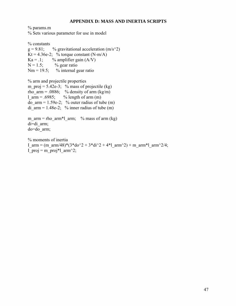
The first step in determining a model was to find the inertia of the system, 0.0131 kg-m2. This was calculated using the provided bodyb.m program, shown in Appendix D. This script calculated important mass and inertia properties when provided with dimensions and variables specific to this system. These variables were determined by both the specification sheet of the motor, Appendix C, or calculated by hand.

4.2 Friction Testing

Friction testing was then administered by using a variety of scripts, included in Appendix E. These scripts were implemented through the Simulink diagram shown in Fig. 1. A series of step voltages were applied to the system. The motor was then allowed to accelerate until a steady state velocity was reached. This velocity was recorded, and the entire series was put onto a plot with steady state velocity on the independent axis and voltage on the dependent axis. The coefficients of static and viscous friction were determined from this plot.

A large number of samples were run, across a range of voltages. This main criteria for the selection of this range was to that it include saturation. Saturation occurs at the voltage where the steady state velocity first hits its maximum value. This effect can be seen in the upper right and lower left corners of Fig. 5. An initial step impulse with a 0.15 second duration was input into the system to break the Coulomb friction. This was necessary because for low voltage inputs, there may be a non-zero steady state velocity if it begins in motion, but not if it begins from rest. This phenomenon is referred to as stiction. After the impulse returned to zero, the

input was a constant value for each tested voltage. To find the friction parameters, the voltage is converted to torque by multiplying by a constant, discussed in detail later in this section.

Fig. 1. Friction ID Testing in Simulink

The position data for each tested voltage was recorded, and used to calculate the velocity

curve at that voltage. Velocity was found by subtracting the current and previous samples, then dividing the sample rate. Fig. 2 shows a sample velocity curve at 0.69 V. The filtered velocity curve was created using a 5th order Butterworth filter. The cutoff frequency was determined experimentally to find a balance between tracking the step input while filtering out the noise. This curve provides an acceptable approximation of the velocity curve. The filtered velocity curve will later be compared to the nonlinear model during model verification.

Fig. 2. Example of Velocity and Filtered Velocity Curves at 0.69 V

It is readily obvious that there is a large amount of noise present in Fig. 2. To filter out the noise, the last 100 samples of the velocity curve were averaged to obtain a steady state

6

velocity. Since the velocity is approaching a steady state value, this method will filter out the undesirable noise, while leaving the desired signal intact. Fig. 3 shows the actual velocity curve and the result of averaging the last 100 samples. It was decided that this method of finding the steady state velocity was acceptable for our data.

Fig. 3: Last 100 Samples of Tilt Velocity Curve

The massive amount of noise in the plot results from a combination of the encoder and the sampling time. Some quantization noise is present in the position due to the resolution of the encoder. The sampling time, however, is the major source of the noise in the velocity. The shorter the sampling time, the smaller the motion that is recorded between samples. A longer sampling time could have been used to increase the frequency resolution and remove much of this noise.

The following graphs displayed as Fig. 4 and Fig. 5 were obtained for the tilt and pan motors, using the steady state velocity determined for every 1/100th of a volt from the method described above:

7

Fig. 4. Friction ID Testing for Tilt Motor

Fig. 5. Friction ID Testing for Pan Motor

8

The graphs in Fig. 4 and Fig. 5 contain two sloped lines each, representing viscous friction, and three vertical lines. The outermost vertical lines indicate the velocity that is saturated at that voltage. The center vertical line represents the Coulomb friction. The main points of interest are the sloped segments. Only the values forming each sloped line were applied to the least squared technique detailed in class, in order to determine the equation for the best fit line. This fitted line is displayed over the sloped section in each figure.

After plotting the steady state versus voltage curve for the tilt axis, an interesting phenomenon was discovered. In the original friction identification with the previous components, specifically 4:1 gearing and a shorter arm, the relationship between voltage and steady state velocity was linear. Fig. 6 below compares the original to the final friction identification plot for the tilt axis. The original friction identification plot has been scaled up in size. With the new data, however, a nonlinear relationship exists between the input voltage and the steady state velocity, seen in Fig. 4. This causes several problems with the friction model that had been used until this point. First, the best fit line does not accurately reflect all of the data points in the region between saturation and Coulomb friction. Second, there is a large discrepancy between the Coulomb friction as determined by the least mean square line and visual inspection. In the right half of Fig. 4, the Coulomb friction has a magnitude of about 0.6V when visual inspection is performed. The best fit line, on the other hand, would suggest a Coulomb friction of around –0.2V. This would later greatly reduce the accuracy of the standard friction model.

Fig. 6: Comparison of Original to Final Friction ID of Tilt Axis

9

While the exact cause of this nonlinearity has not been conclusively determined, some speculation can be made as to its source. The enhanced 3:2 gearing ratio increased the velocities attainable by this system. It is not uncommon for linear systems to deviate from the linear model at higher frequencies due to unmodeled resonances and other high frequency dynamics.

The velocity curves for each motor may then be plotted. The velocity curves for the tilt axis are shown in Fig. 7 below. This plot represents velocity vs. time for varying step inputs. In order to do friction identification, a steady state velocity is needed. One can then look at these plots to confirm that all of the transients have settled into a steady state value. These curves were generated using the Butterworth filter previously described.

Fig. 7. Velocity Curves for Tilt Motor

Using the best fitted line method, the values below were calculated using the Matlab function pinv [5], for the pan motor, by finding the slope and critical points:

⎥⎦⎤

⎢⎣⎡=⎥

⎦

⎤⎢⎣

⎡1481.486.

//

:31

32

aaaa

positive

⎥⎦⎤

⎢⎣⎡−=⎥

⎦

⎤⎢⎣

⎡1129.

543.//

:31

32

aaaa

negative

The following values corresponding to the tilt motor were then calculated using the same

method discussed above (note that the parameters for the tilt axis are not completely accurate as discussed above):

⎥⎦⎤

⎢⎣⎡ −

=⎥⎦

⎤⎢⎣

⎡3130.

1226..//

:31

32

aaaa

positive

10

⎥⎦⎤

⎢⎣⎡=⎥

⎦

⎤⎢⎣

⎡3698.2309.

//

:31

32

aaaa

negative

The a2 /a3 term is the Coulomb friction of the motor; the point where the center vertical line ends, and the sloped line begins. As taken from the figures, it is in units of Volts. The a1/a3 term is the viscous friction of the motor, and is the slope of the fitted line. As taken from the figures, it is in units of V/(rad/s) or Vs/rad. The Coulomb and viscous friction values then need to be converted to N.m and N.ms/rad, respectively. This is accomplished by multiplying each value by the term NNmKTKA, with the value of each element shown in TABLE 2:

TABLE 2: CONSTANT AND GAIN VALUES

N Gear Ratio (tilt; pan) 3/2 ; 4/1 Nm Internal Reduction Ratio 19.5 KT Torque Constant 4.36E-02 N.m/A KA Amplifier Gain .1 A/V

The voltage that is applied to the motor first goes through an amplifier with a gain of KA,

converting the voltage to a current. The current then produces torque in the motor through the internal torque constant, KT. Next, multiplying this torque by NNm yields the friction torque as seen by the load. This constant is calculated to be

VmNvAAmNEKKNN ATm /.12573.0)/1)(./.0236.4)(5.19)(2/3( =−= , and when multiplied by the Coulomb and viscous friction values found previously will

return units of Coulomb: mNVmNV ./. =∗ Viscous: radmsNVmNradVs /././ =∗ , which are the units needed for future calculations. The positive and negative terms for

Coulomb and viscous friction were averaged for each motor, to minimize error obtained during testing. The average values, in bold, were then used in future calculations concerning friction. TABLE 3 summarizes the friction values found during testing.

TABLE 3. FRICTION ID VALUES DETERMINED DURING TESTING

Tilt Motor Pan Motor Coulomb Friction (Positive) 0.0156 N.m 0.1653 N.m Coulomb Friction (Negative) -0.0294 N.m -0.1847 N.m Average Coulomb Friction 0.0225 N.m 0.175 N.m Viscous Friction (Positive) 0.0399 N.m.s/rad 0.0504 N.m.s/rad Viscous Friction (Negative) 0.0472 N.m.s/rad 0.0394 N.m.s/rad Average Viscous Friction 0.0436 N.m.s/rad 0.0449 N.m.s/rad

These frictions values were then incorporated into a complete nonlinear model.

4.3 Trajectory Design and Analysis The trajectory analysis calculations and graphs were implemented in the Matlab script cpathanalysis.m, Appendix F. The script begins by calculating the angular acceleration needed at the throwing radius, rth, using Equation 1.

th

releaserg

=••

θ (1)

11

The minimum angular acceleration needed to launch the ball is then determined to be 12.4 rad/s2. Using the a standard equation of motion (2), where h is the desired vertical height of the ball’s trajectory,

g

vh2

2

= (2)

and dividing by the length of the throwing arm, an equation for the angular velocity needed at the release point is determined:

th

releaser

gh2=

•

θ (3)

For a desired height of 1 meter, it was determined that needed to be 5.6 rad/s. release

•

θ To calculate the release time of the ball, trelease, at which the arm starts decelerating and causes the ball to launch, Equation 4 is implemented, dividing the desired angular velocity by the desired acceleration at the release point.

release

releasereleaset

••

•

=θ

θ (4)

The time at which the ball will be caught is then represented in Equation 5, where vrelease can easily be determined by multiplying the angular release velocity by the rth.

gv

t releasecatch = (5)

The starting position, in radians, is then found using Equation 6. The time is takes to lower to this position is found using Equation 8, derived from a standard equation of motion shown in Equation 7, where the prepared acceleration is an arbitrary value defined in the script.

2

22 releaserelease

start t••

−=θπθ (6)

2

21 atx pos = (7)

prepare

startreverset

••

−=

θ

θπ 2/ (8)

The time at which to begin throwing, tstartthrow, is then arbitrarily decided to be twice treverse in order to allow the user sufficient time to place the ball in the cradle. Using the above calculations, piece-wise calculations were made as shown in Appendix F. The position graph is shown in Fig. 8. It shows the arm initially at a starting position of approximately 1.57 (π/2) rad, followed by a slow decent to the above calculated θstart position. It then quickly advances to in order to throw the ball and return to the horizontal position.

12

Fig. 8: Position vs. Time of Trajectory

The velocity is then plotted as displayed in Fig. 8. As the derivative of the position graph above, one can see that while the arm is lowering, the angular velocity is much less, approximately 1.75 rad/s, than during the period the arm is launching the ball, closer to 6 rad/s.

13

Fig. 9: Velocity vs. Time of Trajectory

Acceleration vs. time is then plotted, Fig. 10, as the derivative of the velocity above. Again, the acceleration during the launch period is much greater than during the lowering period, about 12.4 rad/s2 as calculated in Equation 1.

14

Fig. 10: Acceleration vs. Time of Trajectory

Fig. 11 shows the torque vs. time graph. This graph was plotted taking into account a gear ratio of 3:2 and Equation 9, given in class notes [8].

)sin()sgn( θθθθ

τ cCva gB

gratioB

gratioJ

+++=•

•••

(9)

As seen from the graph, the highest torque is at the end of the signal, at approximately 2.7 seconds. This occurs because the velocity at this point is fairly high, which creates a large back emf which reduces the amount of voltage available to create torque.

15

Fig. 11: Torque vs. Time of Trajectory

Using the data from Fig. 11 and Equation 10 as the boundaries, the feasibility of the required torque need was plotted, shown in Fig. 12.

ττ max

max_max_ speedspeedV −= (10)

16

Fig. 12: Feasibility of Required Torques

A small portion of the velocity versus torque curve crosses one of the feasibility boundaries. Upon further analysis, it was determined that this infeasibility did not affect the system’s performance because it occurred after the launch of the ball. Fig. 13 below plots the position of the arm up until a time soon after the launch.

17

Fig. 13: Shortened Position vs. Time

If the feasibility curve for this time period is then produced, Fig. 14, it can be seen the torque required is feasible while the ball is still in the cradle.

Fig. 14: Shortened Feasibility of Required Torques

18

4.5 Control Signal From our above mentioned trajectory calculations, it was determined that the minimum acceleration and deceleration of the arm would need to be 12.4 rad/s2, the acceleration of gravity times the throwing radius, rth. In order to ensure the ball would be launched sufficiently, a deceleration value of 19 rad/s2 was chosen rather then the minimum value of 12.4 rad/s2.

The control signal calculations were then implemented throughout Matlab script cpath2.m, seen in Appendix G. This script is very similar to cpathanalysis.m, Appendix F, with a few exceptions. As just discussed, the maximum acceleration used was enhanced from 12.4 rad/s2 to 19 rad/s2. In order to easily initialize the system to the same position and retain consistency, the arm was set to start in a downward vertical position. Because of this, the control signal needed to first raise the arm to its horizontal position to allow the user to place the ball in the cradle before recoil and launch. The system then needed to wait in the horizontal position after the launch in order to catch the ball on its way down.

In order to raise the arm from the vertical position to the horizontal position initially, a simple ramp with a constant velocity of π/4 rad/s was added. A second negated ramp is added in order to cancel out the first and allow the system to stay still for 1 second, allowing the user to place the ball in the cradle. This can be seen in the positively sloped line followed by a short horizontal line in the first section of Fig. 15.

The lowering motion before launch was achieved with a relatively slow acceleration of 1.6 rad/s2 in order to keep the ball from falling out of the cradle. This creates an “S” shaped curve with velocities of 0 on either end so there will be no jerkiness, which can be seen in the center section of Fig. 15.

Fig. 15: Desired Position vs. Time of Control Signal

19

As shown in the desired acceleration plot, Fig. 16, there are three discontinuities. These occur at the start and end of the ramp, and after the final deceleration of the arm, due to instantaneous changes in velocity. These discontinuities could have been diminished by creating a higher order control signal in those areas, but this task was never implemented as the effects of them did not affect the projection of the ball. However, when the system was run, such demands for torque that were made on the system at those key points would cause the system to shake, as is seen in the video and various graphs included in the System Performance section later in this report.

Fig. 16: Desired Acceleration of Control Signal

It is noteworthy, although, to mention that the final release point used during implementation was not exactly horizontal. Initially the control signal was defined such that the arm would start decelerating at π/2 rad. This did not result in the ball actually being released at this point because of deceleration issues and overshoot. The release point was then varied to a lower position after the control signal was calculated, in order to confirm a correct departure position of the ball. To accomplish this, two ramps were added to the Simulink diagram. The first ramp brought the arm from 0 rad to the release point, and after 2 seconds the second ramp began, canceling out the first ramp.

As an enhancement to the system, the pan control was implemented in order to rotate approximately π rad and catch a ball that was projected forward. The pan control can be seen in Fig. 17. It is a ramp for simplicity purposes in order to demonstrate its feasibility. It causes the pan motor to rotate π rad at a constant speed of π/2 rad/s in 2 seconds time. In future implementation this signal should be quadratic such that the velocity is 0 rad/s at the start and beginning of the panning motion.

20

Fig. 17: Pan and Tilt Control Signals

4.5 Modeling

Non-linear Model:

The model, Appendix A, begins with an input voltage, which is immediately multiplied by the term NNmKTKA, a constant that is used to convert voltage to torque. The torque produced by the motor has a saturation that is a function of the current velocity of the motor. Because Simulink does not have a variable saturation block, a subsystem was created in order to solve this issue. This subsystem takes inputs of the desired torque and velocity, and outputs a torque saturated to fall under the motor speed-torque curve.

There are two nonlinear effects that are added to the torque produced by the motor to yield the net torque. One of these effects is the gravitational loading, a sinusoidal function of position, while the other is friction, a function of velocity. Once these are added in, a simple double integrator system remains. This represents the dynamics of the transfer function between the net torque and the output position. The integrators are applied one at a time so the acceleration and velocity may be extrapolated as intermediate steps.

With the original configuration of a 4:1 gear ratio for the tilt axis, the friction model consisted of a constant torque (Coulomb friction) plus a torque proportional to the velocity (viscous friction). After the new gears were integrated, bring the gear ratio down to 3:2, the identification profile changed in such a way that the previous friction model was no longer suitable. This was discussed in more detail in Section 4.2.

In performing the model validation, it was found that the friction model being used did not entirely encompass the true behavior of the system. Given the curvature of the plot in Fig. 4, it was obvious that the relationship between velocity and viscous friction torque was nonlinear. One paper suggested that a more accurate model [7] in which the viscous friction is a function of

21

the velocity raised to some power, demonstrated in Equation 11. This was ultimately used in the nonlinear model.

)sgn(vvFF v

vδ= (11)

A problem that has continually arisen in the simulation concerns inputting any voltage value that should not be strong enough to break the Coulomb friction. When this occurs, the simulation takes an extremely long time to process. This was initially attributed to the zero crossing detection built into Simulink. The Coulomb friction causes a discontinuity that is highly susceptible to chattering [6], as shown in Fig. 18.

Fig. 18. Voltage Chattering due to Discontinuity

For small voltage inputs, a non-zero velocity inevitably emerges. The initial solution to

this problem was to disable zero crossing detection, which showed a small amount of improvement, but much was left to be desired. A dead zone was then added immediately before the friction block. It is used to reduce small voltage values to zero, and lessens the significance of the discontinuities from Coulomb friction. Astrom describes a similar technique [7] and is referred to as the Karnopp model. This improved the performance, but at a cost. The simulation can be sped up by increasing the width of the dead zone, but the velocity still chatters. It was determined that the velocity chatters about a value equal to the width of the dead zone. We have yet to determine a method to completely eliminate this problem from the model simulation. It has, although, been determined that if a voltage that is strong enough to break the Coulomb friction is input initially, followed by a voltage value which is not strong enough, the function will behave as it should, in a reasonable amount of time, as shown in Fig. 19.

22

Fig. 19. Voltage Input and Velocity Response for an Initial Voltage of 0.9 V followed by a Voltage of 0.1 V

Linear Model: The linear model was obtained by linearizing the nonlinear model around the point

dθ =π/2, the point at which the arm is horizontal for release of the ball. This is accomplished by substituting calculated values into the second order system represented by Equation 12, given in class lecture [9].

)cos(

1)( 2dv mglsBJs

sGθ−+

= (12)

Thus, the linear model shown below was obtained by plugging J and Bv, calculated in sections 4.1 and 4.2, into Equation 12.

sssG

0204.0131.01)( 2 +

=

4.6 Control Design The linear continuous controller was found by using rltool, displayed in Fig. 20, to move the poles, zeros, and gain around until an optimal bode diagram was found. This diagram would contain a gain drop off such that higher frequencies, such as noise, would be cancelled out, and a minimal phase shift. This bode diagram for the final controller is displayed as Fig. 21, and the continuous controller for the tilt motor is described below as C(s).

1064.141.*80)(++

=s

ssC

23

Fig. 20: Root Locus Plot for Continuous Controller

The bode diagram, Fig. 21, for the open loop system has a gain margin of -368 dB and a phase margin 4.27 degrees. Initially the gain chosen for the controller was too low and caused a phase shift, resulting in a skewed response. This was remedied soon after as seen in Fig. 21 below by increasing the gain constant.

24

Fig. 21: Bode Diagram for Continuous Controller, Open Loop

Once a controller had been selected, it would be tested by examining its response to a impulse, a step, and control signal from cpath.m, Appendix G. These can be seen in Fig. 22. If these responses did not meet our main specification of following the control signal well, the gain was modified to consider what effects that would have. If that did not repair the problem, the bode would be more closely examined and a control would be designed that created a fast or slower response as needed. Two important results were observed. The first is that the step response was critically damped. Second, the control signal has motor follow the signal very closely, except for a little shaking at around 8.75 seconds. This shaking was due to discontinuity in the required torque. The closed loop bode diagram, Fig. 22, found that there was an infinite gain margin, and therefore would not go unstable. It showed a closed loop phase margin of 6.04 degrees, and also that the system canceled out high frequency noise created by the encoder noise.

25

Fig. 22: Continuous Closed Loop Bode Diagram with Impulse, Step, and Simulation Responses

This process was repeated with the linear discrete controller, which was used in the final system. We used the Matlab function c2d to convert the continuous controller, C(s), to a discrete controller. The discrete controller described below as C(z). This controller was then plotted using rltool.

26

9845.0391.6406.6*80)(

−−

=z

zzC

Fig. 23: Root Locus for Discrete Controller

Next, the bode plot, and gain and phase margins of the system were examined as shown

in Fig. 24. The open loop gain margin is -235 DB and the phase margin is 4.26 degrees.

27

Fig. 24: Bode Diagram for Discrete Controller, Open Loop

Its responses to an impulse, step, and control signal from cpath2 were then examined, as shown in Fig. 25. One result is that the step response had a large overshoot of about 80%. Another was that the control signal had motor follow the signal very closely, except for a little shaking at around 8.75 seconds, due to discontinuity in the required torque, as described above. The bode diagram shows that there is now a gain margin of 373 dB and 6.03 deg phase margin. It also shows that the system cancels out high frequency noise that is created by the encoder noise.

28

Fig. 25: Discrete Closed Loop Bode Diagram with Impulse, Step, and Simulation Responses

The system behaved a much better with the continuous controller, but the discrete form still follows our signal well. This ability to follow the control signal well is the most important characteristic to the system.

4.7 Error Analysis The error in the release angle of the arm was critical to the design as it determines at what

position the projectile may land. One must study the maximum allowable error to quantify the maximum error that a motor may have while following a desired path. The diameter of the catching funnel is 0.1016 meters, resulting in a landing position error of 0508.0± meters.

The maximum error of the release angle was determined to by acceptable was found by using the Matlab scripts in Appendix I. This is an error of about 16%. At a 10% increase in velocity, (3.834 m/s)(1.1)=4.2174 m/s, it was determined that the maximum available error in release angle is 15%, only a small reduction from 16%.

Fig. 26 shows the relationship between the error of the release angle and the deviation of the landing position of the projectile, at an initial velocity of 3.834 m/s. This analysis initially seemed valid, although when tests were ran it was found that there was far less room from error than these calculations suggested. Possible causes of the additional error are spin induced on the ball during the launch, or inconsistencies such as tilting and slight changing of shape of the cradle. With increased study of the error factors, the error analysis could have greatly improved.

29

Fig. 26. Deviation in Landing Position of Projectile at 3.834 m/s

4.8 Modifications of the Mechanical System In order to increase the possible angular velocity of the system, two new gears were

purchased in order to decrease the initial 4:1 gear ratio of the tilt motor. The larger gear had a 0.935 inch diameter, while the smaller one had a 0.609 inch diameter, resulting in a 3:2 gear ratio.

In addition, to further increase the angular velocity at which the ball itself would be launched, a longer rod, 0.7400 meters, as opposed to the previous 0.2794 meters, was implemented in the final design.

A new cradle was also implemented in order to minimize the effect of ball bounce. The initial cradle was made of Styrofoam, and caused the ball to bounce out very easily. An attempt at minimizing bounce by angling the walls and padding the bottom with cotton balls was tried to no avail. The new cradle was made with a 4 inch diameter wooden hoop and a slightly elastic fabric pouch, and results were much better.

30

31

5. DESIGN VERIFICATION Discuss the testing and performance verification of the completed project and its major

subprojects. Compare simulation and experimental results. Compare achieved performance with the design specification. Provide solid technical data, and present it in an easily grasped manner, using graphs where possible. Include any test results that you feel are needed to prove that the design goals were met.

5.1 Model Verification In the model verification process, the results of the model simulations for a given input were compared against the actual system response for that same input. The model and its parameters were then iteratively adjusted to improve the validity of the model. It was during this stage that the more accurate friction model was developed.

For a linear system, the verification process is relatively simple. Bode plots can be constructed for both the model and the physical system. Then the poles and zeros of the model can be moved around accordingly. Verifying a nonlinear system is much more complicated because of elements such as saturation and discontinuities. There are also other unmodeled dynamics that act unpredictably.

A challenge arose in finding a systematic way of comparing the simulated and actual responses over a wide range of inputs. Since the friction identification provided a good picture of the steady state behavior of the system for a wide range of input step voltages, this process was simulated on the model. Adjusting the model such that the simulated friction identification match the actual curve served as the basis for creating an accurate nonlinear model. Once the parameters for the tilt axis had been identified from the friction identification process, Fig. 4, it was discovered that the best fit line placed the Coulomb friction at a negative value. Because of this, the Coulomb friction had to be found manually. It took an input of about 0.6V magnitude in order to overcome the static friction. This Coulomb friction was used along with average viscous friction from TABLE 3 in the nonlinear model. The friction identification process was then simulated on the model, as shown in Fig. 27. While the simulated saturation velocity was slightly greater than the actual velocity, the most disconcerting feature was the shape of the curve in the active region, which did not fit the real data.

Fig. 27: Initial Friction Simulation, Tilt Axis

Next, the effect of changing the viscous friction coefficient was investigated, since the slope of the curve was not constant over the active region. Fig. 28 shows the curves for a range of several value of the viscous friction coefficient. There were two main problems with this. First, the curvature of the active region was not captured by any of the simulations. Also, the location of the elbow where the velocity goes into saturation was not reproduced in any of the simulations.

32

Fig. 28: Various Friction ID Simulation Curves, Tilt Axis

At this point, a different model of the friction was required. Astrom [7] discusses the classical friction model. It was suggested that a better fit to experimental data could often be found by a nonlinear dependence on velocity for the viscous friction. The friction model was altered to accommodate for this new description. The exponent on the velocity was then iteratively found to be 1.7. This generated a friction identification curve that very closely matched the actual data, shown in Fig. 29.

33

Fig. 29: Simulated Friction ID on Model

Fig. 30 shows a few actual step responses were also compared to those from simulation. The bottom response is the one with the most deviation between the simulated and actual responses, and it was the one done with smallest step voltage. This would imply that the model is less accurate near the minimum voltage required to break the Coulomb friction.

34

Fig. 30: Model Testing with Various Step Inputs

5.2 System Performance In the end, the system was able to perform well enough to meet the desired specifications. Initially, simple proportional feedback control was used to get a general idea of how the real system would react to the desired trajectory. Fig. 31 shows the desired and actual trajectories with a proportional gain of 100. In that case, limit cycling occurred after release and the arm began shaking. Such a scenario was not very conducive to catching the projectile, so a lower proportional gain was required. However, as the gain was lowered, the system was unable to track the initial drop, where the arm lowered to the pre-release position, without vibrating enough to knock the ball out prematurely. This was largely due to the effects of the Coulomb friction.

35

Fig. 31: Model Using Proportional Control and Kp=100

Next, the discrete controller was used, along with friction cancellation. The friction was cancelled by adding 0.6V multiplied by the sign of the error to the input voltage. This was effective at removing the shaking, and the ball was able to remain in the cradle until the moment of release. A gain of 200 was first tried with the discrete controller but the vibrations were too great, as one can see in Fig. 32. The gain was then lowered to 100, Fig. 33, which produced a much better response. The tracking was good, although there was some overshoot at the end and some steady state error. Because neither of these issues affected the physical performance of the system, they were both deemed to be acceptable.

36

Fig. 32: Model Using Friction Cancellation and Kp=200

Fig. 33: Model Using Friction Cancellation and Kp=100

37

Fig. 34 shows the desired, simulated, and actual trajectories of the system. The simulated overshoot is slightly less than the actual overshoot, but the graph still shows the ability of the model to accurately predict the system’s response.

Fig. 34: Simulation of Input Trajectory

The pan tracking control signal was feed into the motor using the Simulink diagram found in Appendix B. This implemented feedback loop subtracts the desired θ from the actual signal received from the encoder. That value is then multiplied by the gain, Kp, which was set to 50. It is then sent as a voltage command to the motor. The results of this test are shown in Fig. 35. The motor follows the desired trajectory very well with no steady state error, which is very important with regards to catching a ball. The only deviation in the actual trajectory from the desired trajectory was the slight variation in the signal that occurred on the ramp part of the signal. This small divergence is most likely due to Coulomb friction and could be eliminated using the same method described earlier, to add the Coulomb friction times the sign of the input voltage, plus the input voltage to the signal.

38

Fig. 35: Pan Tracking with Kp=50

39

40

6. COSTS AND SCHEDULE

6.1 Costs TABLE 4 below summarizes all costs for the project. The top half of the parts section of the table includes prices on the equipment that was provided at the beginning of the semester. The bottom half are materials purchased throughout the semester in order to enhance and add on to our basic given mechanical model. These parts totaled $67.90, a reasonable price considering our projects goals and mechanical design. Labor hours were based on an average of 200 hours throughout the semester per person. This number was determined by averaging each member’s hours as written in his or her personal design notebook. An approximate total number of shop hours (100), was also determined by calculating hours spent in the shop according to the personal notebooks. Both the rate per hour of each member and the shop time are estimates of what may be charged in a realistic situation.

TABLE 4: COST AND LABOR

Components Manufacturer Part Number Cost Quantity Total Motor Pittman GM8724s016 $112.26 2 $224.52

Large Gear Stock Drive A 6A61-00NF03112

$19.37 2 $38.74

Small Gear Stock Drive A 6A 6-25DF03106

$7.40 2 $14.80

Timing Belt Stock Drive A 6R 6-1150310

$4.12 2 $8.24

Styrofoam Funnel Walmart N/A $1.50 2 $3.00 Miscellaneous

Items Walmart N/A $10.00 1 $10.00

Bore Reducer Stock Drive A 7A30-311806

$5.47 1 $5.47

Timing Belt Stock Drive A 6R 6-1090310

$4.21 1 $4.21

Small Gear Stock Drive A 6A 6-48DF03110

$9.91 1 $9.91

Large Gear Stock Drive A 6A 6-72NF03112

$12.33 1 $12.33

Shipping/ Handling/ Sales Tax

$14.75 $3.95 $4.18

- $22.88

Total Parts: $315.94 Labor and Shop:

Person Cost/hour Hours Total Dan $30 200 $6000 John $30 200 $6000

Shannon $30 200 $6000 Total Labor $18000

Total Shop Hours $50 100 $5000 Total Cost $23,315.94

41

6.2 Schedule TABLE 5 below represents the schedule that our team attempted to follow throughout the semester. It was modified several times throughout the semester due to its vague characteristic. This vagueness also caused our team to fall slightly behind mid semester, although extra hours contributed by each team member during the last few weeks helped us to accomplish our goal for the final presentation.

TABLE 5: SCHEDULE

Task (person) 2/18 2/25 3/3 3/10 3/17 3/24 3/31 4/7 4/14 4/21 4/28 Background Research

Develop Model (John)

Order Parts (All)

Verify Model(All)

Design Control Signal (Dan)

Design Controller (Dan)

Test Controller in Simulink (Shannon)

Test and Refine Controller(All)

Prepare Demo(All)

Write Final Report(All)

42

7. CONCLUSIONS The initial goal of catching a vertical toss was achieved and recorded by videotape. The

system accomplished this goal relatively consistently and effectively. The enhanced goal of using the pan motor to quickly spin around and catch the ball was implemented. This task was more difficult than was initially planned, as the arm was not centered about the tilt axis. This resulted in an offset of about 0.2 meters when the pan axis rotated 180 degrees. With further calculations although, this task may have been accomplished had time permitted.

Some recommendations that could be taken into consideration in the future include using a ball with lower coefficient of restitution, designing a cradle that is stiff, sturdy, and shock absorbing in order to increase consistency of the toss, mounting the throwing arm so that it is centered with the pan axis, and attaching an electric level (inclinometer) to the tilt axis in order to accurately initialize the system. Enhancements that could possibly be implemented in the future include adding sensors to track ball and correct for error, juggling multiple balls at once, extending the original arm so that there is a cradle on each side, and having two separate systems with coordinated activities. Had time permitted, it would have been interesting to discover what else the system was capable of.

43

8. REFERENCES [1] M.K. Raymond, “Pitching Machine Springs into Action,” Machine Design, January

13, 2000, http://www.findarticles.com/cf_dls/m3125/1_72/59461849/p1/article.jhtml [2] J.N. Wilford, “How Catapults Married Sciences With Politics,” New York Times,

February 24, 2004, http://www.ancientworlds.net/aw/Post/274964 [3] J.F. Guilmartin, “Ballistic Weapons,” Houghton Mifflin,

http://college.hmco.com/history/readerscomp/mil/html/ml_005400_ballisticwea.htm [4] Science & Technology, European Space Agency, “Ulysses Launch Information,”

October 6, 1990, http://sci.esa.int/science-e/www/object/index.cfm?fobjectid=33615 [5] J. Wen, “Parameter Identification,” class notes for ECSE 4962, Department of

Electrical, Computer, and Systems Engineering, Rensselaer Polytechnic Institute, Feb. 10, 2004.

[6] MathWorks Documentation, “Using Simulink,” http://www.mathworks.com/access/helpdesk/help/toolbox/simulink/ug/how_simulink_works14.html

[7] K.J. Astrom, et al, “Friction Models and Friction Compensation,” Nov. 28, 1997, http://www.cat.rpi.edu/~wen/ECSE4962S04/astrom_friction.pdf

[8] J. Wen, “Modeling of Dynamical Systems,” class notes for ECSE 4962, Department of Electrical, Computer, and Systems Engineering, Rensselaer Polytechnic Institute, 2004.

[9] J. Wen, “Using MATLAB and Simulink for Control System Simulation and Design,” class notes for ECSE 4962, Department of Electrical, Computer, and Systems Engineering, Rensselaer Polytechnic Institute, 2004.

APPENDIX A: NONLINEAR MODEL INCORPORATING NONLINEAR FRICTION

44

APPENDIX B: PHYSICAL SYSTEM CONTROL, PAN AND TILT

45

APPENDIX C: MOTOR SPECIFICATION SHEET

46

47

APPENDIX D: MASS AND INERTIA SCRIPTS % params.m % Sets various parameter for use in model % constants g = 9.81; % gravitational acceleration (m/s^2) Kt = 4.36e-2; % torque constant (N-m/A) Ka = .1; % amplifier gain (A/V) N = 1.5; % gear ratio Nm = 19.5; % internal gear ratio % arm and projectile properties m_proj = 5.42e-3; % mass of projectile (kg) rho_arm = .0886; % density of arm (kg/m) l_arm = .6985; % length of arm (m) do_arm = 1.59e-2; % outer radius of tube (m) di_arm = 1.48e-2; % inner radius of tube (m) m_arm = rho_arm*l_arm; % mass of arm (kg) di=di_arm; do=do_arm; % moments of inertia I_arm = (m_arm/48)*(3*do^2 + 3*di^2 + 4*l_arm^2) + m_arm*l_arm^2/4; I_proj = m_proj*l_arm^2;

48

% Calculate the mass and inertia properties for body B % Ben Potsaid Jan 21, 2003 % modified February 17, 2004 % Must run params.m first %%%%%%%%%%%%%%%%%%%%%%%%%%%%%%%%%%%%%%%%%%%%%%%%%%%%%%%%%%%%%%%%%%%%%%% % Define some key dimensions and properties of the individual bodies. % %%%%%%%%%%%%%%%%%%%%%%%%%%%%%%%%%%%%%%%%%%%%%%%%%%%%%%%%%%%%%%%%%%%%%%% rho_al = 2.768e3; % density of aluminum (kg/m^3) rho_cf = 8.86e-2; % density of carbon fiber rod (kg/m) dia_hub = 0.0305; % diameter of hub on timing pulley dia_pulley = 0.0472; % outside diameter of timing pulley dia_hole = 0.00953; % diameter of hole in timing pulley thick_hub = 0.00794; % thickness of hub on timing pulley thick_pulley = 0.00794; % thickness of timing pulley thick_hole = 0.00794*2; % thickness of hole in timing pulley %%%%%%%%%%%%%%%%%%%%%%%%%%%%%%%%%%%%%%%%%%%%%%%%%%%%%%%%%%%%%%%%%%%%%%%%% % Calculate position to the COM, mass, and inertia tensor for each body % %%%%%%%%%%%%%%%%%%%%%%%%%%%%%%%%%%%%%%%%%%%%%%%%%%%%%%%%%%%%%%%%%%%%%%%%% % for the skeletal tilt assembly p_skel = [0 0.003 0]'; m_skel = 0.07583; I_skel = [ 0.0001284 0.0 0.0; 0.0 1.470e-6 0.0; 0.0 0.0 0.0001284 ]; % for the hub of the pulley p_hub = [0 -0.0588 0]'; m_hub =rho_al*pi*(dia_hub/2)^2*thick_hub; I_hub = [1/12*m_hub*(3*(dia_hub/2)^2+thick_hub^2) 0 0; ... 0 1/2*m_hub*(dia_hub/2)^2 0 ; ... 0 0 1/12*m_hub*(3*(dia_hub/2)^2+thick_hub^2)]; % for the outside of the pulley p_pulley = [0 -0.0493 0]'; m_pulley =rho_al*pi*(dia_pulley/2)^2*thick_pulley; I_pulley = [1/12*m_pulley*(3*(dia_pulley/2)^2+thick_pulley^2) 0 0; ... 0 1/2*m_pulley*(dia_pulley/2)^2 0 ; ... 0 0 1/12*m_pulley*(3*(dia_pulley/2)^2+thick_pulley^2)]; % for the hole of the pulley p_hole = [0 -(0.0588+0.0493)/2 0]'; m_hole =-rho_al*pi*(dia_hole/2)^2*thick_hole; % Note that hole is negative mass I_hole = [1/12*m_hole*(3*(dia_hole/2)^2+thick_hole^2) 0 0; ... 0 1/2*m_hole*(dia_hole/2)^2 0 ; ... 0 0 1/12*m_hole*(3*(dia_hole/2)^2+thick_hole^2)]; % for the arm p_arm = [(.00475+l_arm/2) -.091 0]'; m_arm = l_arm*rho_cf; I_arm = [(m_arm*(do_arm^2+di_arm^2)/8) 0 0; 0 (m_arm*(3*do_arm^2+3*di_arm^2+4*l_arm^2)/48) 0;

49

0 0 (m_arm*(3*do_arm^2+3*di_arm^2+4*l_arm^2)/48)]; % for the projectile (bouncing rubber ball) p_proj = [(.00475+l_arm) -.091 ((.0159+.0095)/2)]'; m_proj = 5.42e-3; I_proj = [1.13e-4 0 0; 0 1.13e-4 0; 0 0 1.13e-4]; %%%%%%%%%%%%%%%%%%%%%%%%%%%%%%%%%%%%%%%%%%%%%%%%%%%%%%%%%%%%%%%%%%%%%%%%%%%%%%%%%%%%%% % Start off with the skeletal body and add the hub of the pulley to form a composite % % body with new mass center at p_sh, new mass of m_sh, and new inertia tensor about % % p_sh of I_sh. One by one, add the rest of the bodies until all of the bodies in % % body B are included. Note that the hole has been included as a negative mass. % %%%%%%%%%%%%%%%%%%%%%%%%%%%%%%%%%%%%%%%%%%%%%%%%%%%%%%%%%%%%%%%%%%%%%%%%%%%%%%%%%%%%%% % add to form skeletal-hub [p_sh, m_sh, I_sh] = compositebodies(p_skel, m_skel, I_skel, p_hub, m_hub, I_hub); % add to form skeletal-hub-pulley [p_shp, m_shp, I_shp] = compositebodies(p_sh, m_sh, I_sh, p_pulley, m_pulley, I_pulley); % add to form skeletal-hub-pulley-hole [p_b1, m_b1, I_b1] = compositebodies(p_shp, m_shp, I_shp, p_hole, m_hole, I_hole); % add to form skeletal-hub-pulley-hole-arm [p_b2, m_b2, I_b2] = compositebodies(p_b1, m_b1, I_b1, p_arm, m_arm, I_arm); % add to form skeletal-hub-pulley-hole-arm-projectile [p_b3, m_b3, I_b3] = compositebodies(p_b2, m_b2, I_b2, p_proj, m_proj, I_proj); p_b = p_b3; m_b = m_b3; % get inertia about coordinate axes rather than about COM I_b = parallelaxis(p_b3, m_b3, I_b3, zeros(3,1), 0, zeros(3), zeros(3,1)); % refer inertia of motor pulley to load inertia dia_mph = 0.0237; % diameter of hub on motor timing pulley dia_mp = 0.0313; % outside diameter of motor timing pulley thick_mph = 0.00794; % thickness of hub on timing pulley thick_mp = 0.00794; % thickness of timing pulley m_mph = rho_al*pi*(dia_mph/2)^2*thick_mph; m_mp = rho_al*pi*(dia_mp/2)^2*thick_mp; I_mph = [0 0 0; ... 0 1/2*m_mph*(dia_mph/2)^2 0 ; ... 0 0 0]; I_mp = [0 0 0; ... 0 1/2*m_mp*(dia_mp/2)^2 0 ; ... 0 0 0]; m_b = m_b + m_mp + m_mph; I_b = I_b + (I_mph + I_mp)*N^2;

50

APPENDIX E: FRICTION TESTING SCRIPTS % Script for automated parameter identification % - Runs a number of tests and saves the data % - Data analysis handled by another script % March 3, 2004 id_ns = 34; % number of samples to run ss_time = 10; % time to reach steady state (sec) Ts = .001; % sampling time (sec) min_voltage = -1.7; % minimum voltage to test max_voltage = 1.7; % maximum voltage to test theta = zeros(id_ns, ss_time/Ts); timevec = 0:Ts:ss_time-Ts; voltage_step = (max_voltage-min_voltage)/id_ns; % space between samples voltages = [min_voltage:voltage_step:max_voltage-voltage_step]; % voltages for i=1:id_ns disp(i) impulse=5*sign(voltages(i)); tg.P2 = impulse; % tg.P2 is final value for step tg.P5 = voltages(i); % tg.P5 is voltage input tg.P6 = .25; % tg.P6 is step time for second step tg.P8 = impulse; % tg.P8 is final value for second step start(tg); pause(ss_time) stop(tg); pause(1) output = tg.OutputLog; for j=1:min([length(timevec) length(tg.TimeLog)]) theta(i, j) = output(j, 2); end end id_stage2

51

% Script for automated parameter identification % - Calculates theta_dot and x based on Stage 1 % March 3, 2004 clear theta_dot back_samples = 100; % number of derivate samples to find ss velocity theta_dot_ss = zeros(1, id_ns); timevec2 = timevec(1:length(timevec)-1); % find theta_dot for i=1:id_ns dtheta = theta(i, 2:length(theta))-theta(i, 1:(length(theta)-1)); theta_dot(i,:) = dtheta/Ts; end % find theta_dot_ss (steady state velocity for i=1:id_ns for j=length(theta_dot(i,:))-back_samples:length(theta_dot(i,:)) theta_dot_ss(i) = theta_dot_ss(i) + theta_dot(i,j)/back_samples; end end % plot theta_dot_ss versus voltage plot(theta_dot_ss, voltages, 'x') title('Friction ID') xlabel('Steady State Velocity (rad/sec)') ylabel('Step Voltage (V)')

52

% Script for automated parameter identification % - Uses data from id_stage2.m % - Outputs Coulomb and viscous friction % March 3, 2004 min_ssw = .1; % minimum steady state velocity max_ssw = 12; % maximum steady state velocity i=1; while theta_dot_ss(i)<-max_ssw i = i+1; end ni0=i; while theta_dot_ss(i)<-min_ssw i = i+1; end ni1=i; while theta_dot_ss(i)<min_ssw i = i+1; end pi0=i; while theta_dot_ss(i)<max_ssw i = i+1; end pi1=i; A1=ones(ni1-ni0+1,2); A1(:,2)=theta_dot_ss(ni0:ni1)'; B1=voltages(ni0:ni1)'; x1=pinv(A1)*B1; A2=ones(pi1-pi0+1,2); A2(:,2)=theta_dot_ss(pi0:pi1)'; B2=voltages(pi0:pi1)'; x2=pinv(A2)*B2; 'negative voltage' x1 'positive voltage' x2

53

APPENDIX F: TRAJECTORY ANALYSIS % Feasability Analysis of Tilt Trajectory clear all close all %intial conditions h=1.0; % height of throw lengthofarm=.7908; % length of throwing arm g=9.81; % gravity amaxang=g/lengthofarm; %throw ball %derive vrelease from max. height = 0.5 * v * v / g vrelease=sqrt(h*2*g); % final velocity nonangular vreleaseang=vrelease/lengthofarm; % final velocity trelease=(vreleaseang/amaxang); % final time thetarelease=pi/2; % final theta %prepare to catch tprepare_to_catch=vreleaseang/amaxang; %final velocity is 0 %final theta is 0 %catch ball thetacatch=thetarelease; tcatch=vrelease/g; %velocity at catch is zero(0) %recoil part 1 accprepare=1.6; %arbitrary thetastart=pi/2-amaxang/2*trelease^2; treverse=sqrt((pi/2-thetastart)/2/(accprepare/2)); %recoil part 2 tstartthrow=2*treverse; %final velocity is zero(0) %final theta is thetastart %throw and catch times with previous times added data trelease=trelease+tstartthrow; tprepare_to_catch=tprepare_to_catch+trelease; tcatch=tcatch+tprepare_to_catch; %time ts=.001; t=0:ts:10; %recoil calculations for i=1:length(t)

54

if(t(i)<=treverse) p(i)=pi/2-accprepare/2*t(i)^2; else if(t(i)<=tstartthrow) ttemp=t(i)-treverse; p(i)=accprepare/2*ttemp^2-accprepare*treverse*ttemp+(pi/2-thetastart)/2+thetastart; else if(t(i)<=trelease) ttemp=t(i)-tstartthrow; p(i)=thetastart+amaxang/2*ttemp^2; else if(t(i)<=tprepare_to_catch) ttemp=t(i)-trelease; p(i)=thetacatch+vreleaseang*ttemp-amaxang*ttemp^2; %catch end end end end end %plot position plot(t(1:length(p)),p) title('Position vs. Time') xlabel('Time (s)') ylabel('Position (rad)') figure %plot velocity plot(t(1:length(p)-1),diff(p)/ts) vel=diff(p)/ts; title('Velocity vs. Time') xlabel('Time (s)') ylabel('Angular Velocity (rad/s)') figure %plot acceleration plot(t(1:length(p)-2),diff(diff(p))/ts^2) accl=diff(diff(p))/ts^2; title('Acceleration vs. Time') xlabel('Time (s)') ylabel('Angular Acceleration (rad/s^2)') figure %plot torque big_gear=.935; small_gear=0.609; gearRatio=big_gear/small_gear J=1.273E-03 ; Bc= 0.1878; Bv=0.0204; gc=.07*-9.8*.79 Torque=J.*accl/gearRatio+Bv.*vel(1:length(accl))/gearRatio+Bc.*sign(vel(1:length(accl)))+gc.*sin(p(1:length(accl))); plot(t(1:length(Torque)),Torque) xlabel('Time (s)')

55

ylabel('Torque (N.m)') title('Torque vs. Time') figure %plot torque feasibility plot(Torque,vel(1:length(Torque))) xlabel('Velocity (rad/s)') xlabel('Torque (N.m)') title('Velocity vs. Torque') hold on; T=0:.001:.83; plot(T,24.1-24.1/8.3e-1*T,'r'); T=-.83:.001:0; plot(T,-24.1-24.1/8.3e-1*T,'r'); xlabel('Torque (N.m)'); ylabel('Velocity (rad/s)'); title('Feasibility of Required Torques'); hold off

56

APPENDIX G: CONTROL SIGNAL % Generates tilt trajectory for vertical throw % Outputs are intilt and inpan %initial conditions h=.5; % height to throw the ball lengthofarm=.74; % length of throwing arm amaxang=19; % max. acceleration from calculations g=9.8; % gravity %throw ball vrelease=sqrt(h*2*g); % final velocity nonangular thetarelease=pi/2; % final theta vreleaseang=vrelease/lengthofarm; % final velocity trelease=(vreleaseang/amaxang); % final time %prepare to catch tprepare_to_catch=vreleaseang/amaxang; %final velocity is 0 %final theta is 0 %catch ball thetacatch=thetarelease; tcatch=vrelease/g; %velocity at catch is zero(0) %recoil part 1 accprepare=1.6; thetastart=pi/2-amaxang/2*trelease^2; treverse=sqrt((pi/2-thetastart)/2/(accprepare/2)); %recoil part 2 tstartthrow=2*treverse; %final velocity is zero(0) %final theta is thetastart %throw and catch times with previous times added data trelease=trelease+tstartthrow; tprepare_to_catch=tprepare_to_catch+trelease; tcatch=tcatch+tprepare_to_catch; %time ts=.001; t=0:ts:10;%tcatch; % % %recoil for i=1:length(t) if(t(i)<=treverse) p(i)=pi/2-accprepare/2*t(i)^2; else if(t(i)<=tstartthrow)

57

ttemp=t(i)-treverse; p(i)=accprepare/2*ttemp^2-accprepare*treverse*ttemp+(pi/2-thetastart)/2+thetastart; else if(t(i)<=trelease) ttemp=t(i)-tstartthrow; p(i)=thetastart+amaxang/2*ttemp^2; else if(t(i)<=tprepare_to_catch) ttemp=t(i)-trelease; p(i)=thetacatch+vreleaseang*ttemp-amaxang*ttemp^2; % %catch else if(t(i)<=6) p(i)=thetacatch; end end end end end end p=(-pi/2+p); p1=[zeros(1,4000) p]; intilt=[t' p1']; inpan=[0 0];

58

APPENDIX H: CONTROLLER DESIGN % Controller Design for Tilt Axis close all % initial parameters J=1.31e-2; % inertia (kg-m^2) Bv=.0204; % viscous frition (N-m-sec/rad) marm=.6985*.0886; % mass of throwing arm (kg) mproj=5.43e-3; % mass of projectile (kg) mcatcher=0; % mass of catcher (kg) m=marm+mproj+mcatcher % total mass l=.6985; % length of arm g=-9.8; % gravity thetad=pi/2; % desired angle c=m*g*l*cos(thetad); % constant gravity loading term ts=.001; % sampling time % set up linear system G2=tf(1,[J,Bv,c]); % linear plant C2=tf([.41,1],[.064,1])*80; % linear controller sys2=C2*G2/(1+C2*G2); % feedback system % plot step and impulse responses figure(1) impulse(sys2) figure step(sys2) figure margin(sys2) figure % get tilt trajectory and simulate it cpath_tilt lsim(sys2,p1,t) %design % desiredpoles; % observerpoles; % G2ss=ss(G2); % [A,B,C,D]=ssdata(G2ss) % F=place(G2ss,desiredpoles) % L=place(A',C',observerpoles)'; % K2controllerss=ss(A-B*F-L*C,L,F,0) % K2controller=tf(K2controllerss) %pan % J=.0146; %kg-m^2 %inertia % Bv=.0276; %viscous frition % thetad=0; % ts=.00042; %sampling time % G1=tf(1,[J,Bv,0]) % figure

59

% impulse(G1); % figure % step(G1) % figure % pzmap(G1) % figure % margin(G1) % figure % discretize continuous plant controller Cd2=c2d(C2,ts) Gd2=c2d(G2,ts,'tustin'); % create discrete feedback system sys2d=Cd2*Gd2/(1+Cd2*Gd2); % plot impulse and step responses for discrete system figure impulse(sys2d); figure step(sys2d) figure %pzmap(sys2d) %figure margin(sys2d) figure lsim(sys2d,p1,t) %rltool(G2)

60

APPENDIX I: ERROR CALCULATIONS %%%%%%%%%%%%%%%%%%%%%%%%%%%%%%%%%%%%%%%%%%%%%% % findthetaerror.m %%%%%%%%%%%%%%%%%%%%%%%%%%%%%%%%%%%%%%%%%%%%%% clear all; i=1; t=-.3:.001:.3; for i=1:length(t) [xdvec(i),y0(i),t_error(i)]=projmotionerror(t(i)+pi/2); end plot(t,xdvec); projmotionerror(pi/2); %%%%%%%%%%%%%%%%%%%%%%%%%%%%%%%%%%%%%%%%%%%%%%% projmotionerror.m %%%%%%%%%%%%%%%%%%%%%%%%%%%%%%%%%%%%%%%%%%%%%% function [xdir,y0,t_error]=error(theta) v0=3.834; y=0; %theta=pi/2-.1; lenghtofarm=.6985;%meteres %error and launch angle calculations t_error=pi/2-theta; direction=sign(t_error); l_ang=pi/2-t_error; %%find launch height y0=-lenghtofarm*sin(t_error); % v0=8.4 % y=0 % y0=150 % l_ang=20/180*pi; %%%%%%%%%%%%%%%%%% %projectile motion v0x=cos(l_ang)*v0; v0y=sin(l_ang)*v0; vy=sqrt(v0y^2-2*9.8*(y-y0)); t=(vy-v0y)/(-9.8); x=v0x*t+0; %%%%%%%%%%%%%%%% %direction of x xdir=x*direction; maxheight=v0y*t/2;

61

APPENDIX J: CONTRIBUTION OF TEAM MEMBERS John Carpenter Nonlinear model, friction identification, nonlinear friction analysis, chattering analysis ____________________________ Shannon Jordan Mechanical system design, modifications of mechanical system, trajectory analysis, format report ____________________________ Daniel Grover Trajectory analysis, control signal, controller design and tuning ____________________________