control system theory in maple - mathematics and computer
TRANSCRIPT
Control System Theory in Maple
by
Justin M.J. Wozniak
A thesis
presented to the University of Waterloo
in fulfilment of the
thesis requirement for the degree of
Master of Mathematics
in
Computer Science
Waterloo, Ontario, Canada, 2008
c©Justin M.J. Wozniak 2008

I hereby declare that I am the sole author of this thesis.
I authorize the University of Waterloo to lend this thesis to other institutions
or individuals for the purpose of scholarly research.
I further authorize the University of Waterloo to reproduce this thesis by pho-
tocopying or by other means, in total or in part, at the request of other institutions
or individuals for the purpose of scholarly research.
ii

The University of Waterloo requires the signatures of all persons using or pho-
tocopying this thesis. Please sign below, and give address and date.
iii

Abstract
In this thesis we examine the use of the computer algebra system Maple for
control system theory. Maple is an excellent system for the manipulation of expres-
sions used by control system engineers, but so far it is not widely used by the public
for this purpose. Many of the algorithms in Maple were implemented because their
application in control theory is known, but this functionality has not been compiled
in a meaningful way for engineers. Over the past two years we have investigated
what functionality control system engineers need and have attempted to fill in the
gaps in Maple’s functionality to make it more useful to engineers.
iv

Acknowledgements
I would like to thank my supervisor, Dr. George Labahn, for his assistance and
guidance in preparing this thesis. I also extend thanks to the readers, Dr. Justin
Wan and Dr. Keith Geddes, whom I met in the classrooms of this university.
A special debt of gratitude is owed to Venus, who accompanied me on our
extended honeymoon in Waterloo this summer. Thank you for your patience during
this project.
I would like to thank Shannon Puddister for his input regarding the user inter-
face from an engineering perspective.
Thanks also to the Symbolic Computation Group, Waterloo Maple and ORCCA,
for financial and academic support.
v

Dedication
This thesis is dedicated to all the family scientists and engineers, especially my
parents, Wayne and Susan.
vi
Contents
1 Introduction 1
1.1 Symbolic Computation and Control System Theory . . . . . . . . . 2
1.2 Existing Software for Control System Theory . . . . . . . . . . . . . 4
1.2.1 MATLAB . . . . . . . . . . . . . . . . . . . . . . . . . . . . 4
1.2.2 Mathematica . . . . . . . . . . . . . . . . . . . . . . . . . . 6
1.2.3 Maple . . . . . . . . . . . . . . . . . . . . . . . . . . . . . . 7
1.3 Thesis Summary . . . . . . . . . . . . . . . . . . . . . . . . . . . . 8
2 Mathematical Background 10
2.1 Control System Theory . . . . . . . . . . . . . . . . . . . . . . . . . 10
2.2 Differential Systems . . . . . . . . . . . . . . . . . . . . . . . . . . . 11
2.3 Linear Time Invariant Systems . . . . . . . . . . . . . . . . . . . . 12
2.3.1 Linearization . . . . . . . . . . . . . . . . . . . . . . . . . . 14
2.4 Output . . . . . . . . . . . . . . . . . . . . . . . . . . . . . . . . . . 15
2.5 SISO Systems . . . . . . . . . . . . . . . . . . . . . . . . . . . . . . 17
2.5.1 Mathematical Description . . . . . . . . . . . . . . . . . . . 17
2.6 Algebraic Operations . . . . . . . . . . . . . . . . . . . . . . . . . . 20
vii

2.7 System Poles and Zeroes . . . . . . . . . . . . . . . . . . . . . . . . 21
3 Basic Analysis 24
3.1 Design Considerations . . . . . . . . . . . . . . . . . . . . . . . . . 24
3.1.1 Graphical User Interface . . . . . . . . . . . . . . . . . . . . 25
3.1.2 Functionality . . . . . . . . . . . . . . . . . . . . . . . . . . 26
3.2 Basic Functions . . . . . . . . . . . . . . . . . . . . . . . . . . . . . 26
3.2.1 System Conversion . . . . . . . . . . . . . . . . . . . . . . . 26
3.2.2 Observability and Controllability . . . . . . . . . . . . . . . 27
3.2.3 Hurwitz Test . . . . . . . . . . . . . . . . . . . . . . . . . . 28
3.3 Graphical Output . . . . . . . . . . . . . . . . . . . . . . . . . . . . 32
3.3.1 Time Domain Response . . . . . . . . . . . . . . . . . . . . 32
3.3.2 Root Locus . . . . . . . . . . . . . . . . . . . . . . . . . . . 34
3.3.3 Nyquist Diagram . . . . . . . . . . . . . . . . . . . . . . . . 36
3.3.4 Bode Diagram . . . . . . . . . . . . . . . . . . . . . . . . . . 38
4 The Matrix Exponential 40
4.1 Definitions and Properties . . . . . . . . . . . . . . . . . . . . . . . 40
4.2 Computation . . . . . . . . . . . . . . . . . . . . . . . . . . . . . . 43
4.2.1 Polynomial Methods . . . . . . . . . . . . . . . . . . . . . . 43
4.2.2 Matrix Decomposition Methods . . . . . . . . . . . . . . . . 48
4.3 Special Cases . . . . . . . . . . . . . . . . . . . . . . . . . . . . . . 51
5 Feedback Control 54
5.1 Ackermann’s Method . . . . . . . . . . . . . . . . . . . . . . . . . . 56
viii

5.2 Direct Method . . . . . . . . . . . . . . . . . . . . . . . . . . . . . . 57
5.3 Transfer Function Method . . . . . . . . . . . . . . . . . . . . . . . 58
5.4 Eigenvector Control . . . . . . . . . . . . . . . . . . . . . . . . . . . 61
6 Conclusion 62
Bibliography 64
A The CST Module 66
B Vita 76
ix

List of Tables
2.1 Algebraic constructions of systems. . . . . . . . . . . . . . . . . . . 21
3.1 Possible inputs for system response. . . . . . . . . . . . . . . . . . . 33
x

List of Figures
3.1 Timing results of two Hurwitz algorithms. . . . . . . . . . . . . . . 30
3.2 Possible uses of the plotting functionality. . . . . . . . . . . . . . . 33
3.3 Possible uses of the root locus functionality. . . . . . . . . . . . . . 35
3.4 Possible uses of the Nyquist functionality. . . . . . . . . . . . . . . 37
3.5 Possible uses of the Bode diagram functionality. . . . . . . . . . . . 39
xi

Chapter 1
Introduction
Control system theory is a broad field that uses many different areas of mathemat-
ics. Differential equations, matrix manipulation, complex functions and integral
transforms are just some of the mathematical tools commonly used in most basic
control problems.
The Maple computer algebra system is an excellent tool to use when approaching
these types of problems, and the engineer attempting to solve a control problem
with Maple would have access to all the functionality necessary. However, Maple
was not designed primarily for engineering applications, and as a result engineers
often use other more specialized software to meet their needs.
The typical modern control system engineer has probably used a system that
emphasizes floating point computation, often in matrix-vector form. Older control
software written in Fortran or C++ would fit into this category, as would modern
MATLAB control software. Such systems tend to emphasize the state-space models
of control systems in a floating point domain.
1

CHAPTER 1. INTRODUCTION 2
In general, Maple’s floating point functionality is slower than that of competing
software, but its polynomial arithmetic and related functionality make up the well-
established, mature parts of the system. This indicates that Maple is best suited
to operate on polynomial models of control systems in exact arithmetic.
In this thesis we have undertaken two projects. The first is to implement in
Maple the basic control system functionality that would benefit the control sys-
tem engineer. This includes convenient plots, graphics, and engineering operations
commonly used in control theory. The second project examines some algorithms
already in Maple that are useful to the engineer, and report on how they help or
hinder control engineering.
We have approached the first project by designing and implementing the CST
package in Maple. This package has a library of software algorithms commonly
used by control engineers. It also has a Maplet that provides easy access to the
graphical routines in the library.
We have approached the second project by investigating two specific computa-
tional problems: solving the homogenous 1st order matrix differential equation and
eigenvalue assignment.
1.1 Symbolic Computation and Control System
Theory
An important issue when developing engineering software for Maple is the differ-
ence between exact arithmetic and floating point arithmetic. Maple is well suited

CHAPTER 1. INTRODUCTION 3
to perform calculations with integers, fractions of integers, algebraic numbers and
unknown parameters. However, a cursory examination of any control theory text-
book will show that engineers prefer floating point computation. Measurements
and constants found in typical electrical or mechanical control systems rarely take
on integer values.
In addition, many computations used in engineering applications do not result
in answers that are easy to describe using exact arithmetic. For example, the
basic analysis of a 5th order differential system involves finding the roots of a 5th
degree polynomial. Although polynomial arithmetic is convenient in Maple, finding
the explicit roots of such a polynomial is not generally possible. However, if the
coefficients are considered floating point numbers, floating point solutions can easily
be found.
Floating point numbers have certain drawbacks, however. Polynomials of 5th
degree or higher may have simple factorizations, especially for systems that were
designed with pole placement techniques. However, even minor round-off devi-
ations from the factorizable polynomial coefficients will result in a factorization
significantly different from the correct answer.
In addition, numerical instability can prevent accurate results from being ob-
tained. For example, manipulation of polynomial matrices in floating point is often
unreliable and computationally expensive [4].
We will assume, then, that the systems of interest to the engineer studying
control theory in Maple will really be investigating control theory, that is, computing
with idealized systems that make for convenient computation. The engineer will be

CHAPTER 1. INTRODUCTION 4
able to gain deep insight into such systems by examining them from a theoretical
perspective.
Graphical output will still be handled through floating point computation as
that is the natural vehicle for plotting, etc. However, important data points such
as maxima, roots, and limits may still be computed exactly if possible.
1.2 Existing Software for Control System Theory
We begin with an examination of popular software tools for the analysis of control
systems. We have chosen to examine three general purpose software systems which
offer potential benefit to the control system engineer.
1.2.1 MATLAB
MATLAB is a popular mathematical programming language based on matrix com-
putation in the floating point domain. MATLAB also offers certain Maple func-
tionality through the “Symbolic Toolbox”. It offers an interactive command-line
interface, and provides a variety of plotting and graphical functionality in pop-up
windows. MATLAB consists of the main program, with a variety of Toolboxes
associated with it that may be used for different applications. It is probably the
most common choice for engineers working with control systems.
The MATLAB Control System Toolbox allows for the creation and manipulation
of Linear Time Invariant (LTI) objects, a MATLAB data type. These objects
may be instantiated using a transfer function format or a state space model. LTI
objects may also be created by pole placement methods or even through graphical

CHAPTER 1. INTRODUCTION 5
pole placement. Model conversion and extraction is possible. LTI objects may be
added, multiplied, and concatenated easily with overloaded arithmetic operations.
Graphical analysis is available, such as the Bode diagram, the Nyquist diagrams,
and the Nichols chart. Time domain responses are available for impulse or step
inputs.
MATLAB’s Robust Control Toolbox is an additional collection of functions for
the design of control systems. This Toolbox contains functions for so-called H2 and
H∞ control, singular value analysis, and Riccati equation tools.
A software tool for MATLAB called Simulink is a graphical tool for the con-
struction and analysis of control systems. This tool allows the user to draw out the
desired system using a GUI, and then perform simulations of system response. The
systems may be continuous or discrete with respect to time, and may be linear or
nonlinear.
Third party software for MATLAB is abundant. For example, Shinners [12]
provides freeware for use by readers of his textbook, called the Modern Control
System Theory and Design Toolbox. This is a general-purpose package of control
functionality that is based around the textbook. It has a full set of graphical
routines as well as some analytical routines, including a small set of polynomial
arithmetic functionality.
Other third party software for MATLAB may be more specialized. For ex-
ample, the Submarine Control Toolbox allows the user to design and simulate a
virtual submarine. Typical design tools are present, including feedback control and
eigenvalue assignment. The resulting design may be previewed in an impressive 3D

CHAPTER 1. INTRODUCTION 6
graphical interface.
1.2.2 Mathematica
Mathematica is a programming language designed for a variety of mathematical ap-
plications in a symbolic context. The kernel of the Mathematica system is designed
for list-based functional programming, but has been expanded to support a variety
of programming styles. Users often prefer the document-driven interface, which is
beneficial for plotting and interactive development, but the kernel is also accessible
from the command line, or from other software systems, such as C, World Wide
Web interfaces, or even Microsoft Excel. Mathematica is distributed by Wolfram
Inc.
Wolfram also offers software called the Control System Professional that is dis-
tributed separately from Mathematica. This software provides a variety of control
functionality and analysis, such as plots and simulation. This functionality is avail-
able inline with the document-driven interface, allowing for seamless development
with other problems. It allows for symbolic analysis of systems such as solving state
equations, numerical system simulation, and classical plotting capabilities like Bode
and Nyquist. Other available plotting includes time domain response to impulse,
step, and ramp input.
Control System Professional also allows for more advanced mathematics, such
as Ackermann’s formula for eigenvalue assignment. Traditional and robust pole
assignment methods are also available. A variety of system realizations may be
computed, including Jordan and Kalman forms. Using such realizations, the order
CHAPTER 1. INTRODUCTION 7
of the system may be reduced to a more convenient form.
For nonlinear systems, linearization or rational polynomial approximation of
nonlinear systems is possible.
1.2.3 Maple
Maple is a computer algebra system designed originally for exact arithmetic and
polynomial manipulation [7]. It is built on a small kernel architecture with a large
library of mathematical functionality which may be loaded when necessary by the
user. Maple is a mature system with widely respected functionality for symbolic in-
tegration and summation, polynomial arithmetic and factorization, number theory,
and multiple-precision arithmetic. Maple has a document-driven interface which
allows access to the kernel, and provides a variety of plotting capabilities.
Floating point computation is performed explicitly by the user with special
commands that allow for arbitrary precision computation. Hardware based floating
point computation is also available, resulting in a fixed precision result but with
more efficient performance.
A recent addition to Maple is the Maplets package, which provides access to
Java-based graphical user interfaces. This allows the programmer to build mathe-
matical applications that the user would be comfortable using, complete with text
boxes, buttons, plots and images.
Although Maple does not yet have a package for control system theory, it does
already provide a great deal of functionality that is important when working on
control problems. Maple allows for elegant handling of the mathematical data
CHAPTER 1. INTRODUCTION 8
types essential for system analysis, such as transfer functions and lists of matrices.
In addition, many mathematical operations important in control system design are
present, such as the Laplace transform, z-transform, and matrix exponential.
1.3 Thesis Summary
In this thesis we will discuss many of the issues involved in using Maple for control
system computation. We will follow a control system design method:
• Chapter 2 - Mathematical Background
Given a system, we must describe it mathematically. We will provide a math-
ematical background for many control system problems. Similarly, the system
must be defined in a computational setting, so we will discuss how to express
such systems in Maple.
• Chapter 3 - Basic Analysis
The control engineer commonly seeks to control some given system, called
the plant. Basic analysis must be performed to determine the properties of
the given plant, such as system response, stability, and error. In this chapter
we will discuss our implementation of some of the simpler control algorithms
and graphical tools.
• Chapter 4 - The Matrix Exponential
It may be desirable to express the response of the system as a function of
time. This involves the computation of the matrix exponential. In Chapter
CHAPTER 1. INTRODUCTION 9
4 we examine a variety of algorithms to handle this problem.
• Chapter 5 - Feedback Control
Given a plant and a desired system behavior, we may design a feedback con-
troller to control the plant so it meets the design criteria. Feedback controllers
can modify the eigenvalues of the closed-loop system. We examine methods
to perform this computation in Chapter 5.
• Conclusion - Chapter 6
We conclude the thesis, tying together the theory and software.

Chapter 2
Mathematical Background
In this chapter we present the mathematical background for the study of control
system theory. We first discuss how to describe a system plant as a differential equa-
tion, and how such systems may be represented in Maple. We then describe some
preliminary operations and analysis, including system synthesis and root analysis.
2.1 Control System Theory
Control system theory is the mathematical process of designing a machine to control
another machine. The machine to be controlled is, in engineering lingo, called the
plant. The machine doing the controlling is called the compensator, or simply the
controller. Each of these machines may be referred to as a system. These two
machines must be somehow connected, output to input, so that they may interact.
We speak of control system theory as a mathematical process because there are
design decisions to be made using mathematical tools, working with idealized math-
10

CHAPTER 2. MATHEMATICAL BACKGROUND 11
ematical models of the actual systems. A mathematical model of a given system
may, for example, be a system of differential equations, with state variables repre-
senting the state of the system. These state variables describe the inner workings
of the machine at hand; for example, positions of components in space, velocities
of components, etc. The input to the system may be described as another set of
independent state variables, and the output of the system may be described as some
function of all the state variables.
With such an abstract concept of systems, we may describe anything from a
microscopic pair of transistors to a gigantic water reservoir. The state variables
for such systems may represent electrons, energy, or gallons of water. Input and
output may occur over silicon circuitry or PVC piping and evaporation.
2.2 Differential Systems
In this thesis we will focus on systems that can be described mathematically by
systems of continuous differential equations. We will assume that the system has
n state variables of interest, as well as n possible inputs. The state variables of
this system will be contained in the vector x, the inputs to the system will be
another vector u, and the time will be denoted t. The change in the state variables
of such a system with respect to time can then be written as x. We will assume
that changes in x are only due to the current values of x, u, and t. With these
assumptions, we can write that the change in x is some function of x, u, and t,
called the system dynamics function, f . With this in mind, we can write a simple

CHAPTER 2. MATHEMATICAL BACKGROUND 12
differential equation
x = f(x,u, t). (2.1)
as a description of our control system.
This is the most general of first-order differential equations; we have no condi-
tions on what kind of function f may be.
2.3 Linear Time Invariant Systems
The systems of concern to us in this chapter are known as linear time-invariant
(LTI) systems. An LTI system has many special properties that allow us to analyze
the system, predict behavior, and control the system. Many of the tools that are
described later in this thesis are only useful for LTI systems.
Time-invariance simply means that time is not a factor in the dynamics of
the system, and that the system dynamics function does not change with time.
Mathematically, this means that we may drop t from equation (2.1) and write:
x = f(x,u). (2.2)
It should be noted that dropping t from this equation does not limit us function-
ally at all, since time can still be considered a factor. Time may still be deduced
in some cases from a component of the input vector, u, or even from certain state
variables in x. Thus, any system of the form (2.1) may be described by a system
of the form (2.2).
Up to this point, we have been referring to the current states of the system.

CHAPTER 2. MATHEMATICAL BACKGROUND 13
Since x and u may change with time, it is preferred to express them as functions of
time, x(t) and u(t). So we will consider x(t) to be the vector of state variables of
x at time t, and u(t) to be the input to the system at time t. We may then write
our differential equation as:
x(t) = f(x(t),u(t)). (2.3)
Linear systems are systems like (2.2), but where the change in state at a given
time is a linear function of both the state and input. This means that the change
in each state variable is equal to the sum of fixed proportions of the state and input
variables, and the input. The proportions will be written as coefficients Aij. An
LTI system has a similar matrix B defined to operate on u. Thus the change in
each state variable can be written as below for a given state variable, xi:
xi(t) =Ai1x1(t) + Ai2x2(t) + ... + Ainxn(t)+ (2.4)
Bi1u1(t) + Bi2u2(t) + ... + Binun(t). (2.5)
The complete linear system may then be written in matrix-vector form:
x1(t)
x2(t)
...
xn(t)
=
A11 A12 ... ... A1n
A11 A11 ... ... A2n
......
...
An1 An2 ... ... Ann
x1(t)
x2(t)
...
xn(t)
+
B11 B12 ... ... B1n
B11 B11 ... ... B2n
......
...
Bn1 Bn2 ... ... Bnn
u1(t)
u2(t)
...
un(t)
,
(2.6)

CHAPTER 2. MATHEMATICAL BACKGROUND 14
or in a condensed form:
x(t) = Ax(t) + Bu(t). (2.7)
2.3.1 Linearization
LTI systems are convenient to work with and easy to describe, but many systems are
not presented in such an easy fashion. Many problems in control system theory are
presented in a more general, nonlinear form, as in equation (2.3). Often, however,
we may approximate such systems by a linear system, by linearizing the system
around a given operating state.
In order to linearize a system, we first pick a state around which to linearize,
for example, an equilibrium point. An equilibrium point is a state x∗,u∗ such that:
f(x∗,u∗) = 0, (2.8)
and has the property that when a system is at the equilibrium point, it will stay
there forever (since then x = 0).
Because f is continuous, we can assume that values of f at x, u close to x∗,u∗
will be close to 0. Linearization is the additional assumption that f will change
linearly as we move away from x∗ and u∗. We can think of this as a truncated
Taylor series representation of f . If f has a Taylor series, and starts at 0, we can
truncate the series so that only the first derivative remains. We assume that this
is appropriate for some range of values close to x∗ and u∗.
Of course, f is a function in R2n → Rn, so we need more than just a standard
Taylor series.

CHAPTER 2. MATHEMATICAL BACKGROUND 15
First, we must assume that x and u affect f linearly with respect to each other,
so that we may approximate f by some functions f1, f2:
f(x(t),u(t)) = f1(x(t)) + f2(u(t)) (2.9)
To get the first derivative in this space, we take the Jacobian of f1 with respect
to x, denoted ∂f1
∂x. Evaluating
∂f1
∂x
∣
∣
∣
∣
x∗
= A (2.10)
gives us our linear operator on x as above in equation (2.7), which will suffice as
an approximation to f1. The second part of (2.9), f2, must also be linearized. We
will linearize the action of f2 on each ui without respect to any uj, j 6= i. This will
give us a matrix B, that may be inserted into (2.7), giving our linearized version
of (2.3):
x(t) = Ax(t) + Bu(t). (2.11)
2.4 Output
The output of a system is the observable data coming back out from the system.
Often, the output of the system is not the same as x(t), the system state, perhaps
because the plant cannot be observed directly, or perhaps because the engineer is
only interested in some subset of the state variables. In such systems, the equation
(2.3) will be a system of two equations, where the output y(t) is represented as

CHAPTER 2. MATHEMATICAL BACKGROUND 16
another function of x(t),u(t). Thus we have:
x(t) = f(x(t),u(t)), (2.12)
y(t) = g(x(t),u(t)).
In some cases, only y(t) may be observed. In this case, if we desire to know
the values of x(t), we will have to estimate their values with an estimator. This is
especially important in feedback control as will be seen later in this thesis.
In equation (2.12) we have f, g written as nonlinear functions. We have already
shown that f may be linearized as in equation (2.11), and g will be linearized in a
similar way.
We first linearize g with respect to x by taking the Jacobian and evaluating at
an equilibrium point x∗.
∂g
∂x
∣
∣
∣
∣
x∗
= C. (2.13)
We then similarly linearize g with respect to u
∂g
∂u
∣
∣
∣
∣
x∗
= D. (2.14)
So our linearized system with input u and output y is
x(t) = Ax(t) + Bu(t), (2.15)
y(t) = Cx(t) + Du(t).

CHAPTER 2. MATHEMATICAL BACKGROUND 17
2.5 SISO Systems
Thus far, we have seen first-order nonlinear and linear systems in n variables.
However, many common systems may have only one state variable in a higher-
order differential equation. Such a system with only one input and one output may
be represented as a SISO (single-input-single-output) system.
2.5.1 Mathematical Description
A linear time-invariant SISO system is described below. Letting u be the system
input, x be the state of the system and y the output, we may describe an nth order
LTI system by a single differential equation:
u(t) = a0x(t) + a1x(t) + ... + an−1x(n−1)(t) + anx
(n)(t) (2.16)
y(t) = c0x(t) + c1x(t) + ... + cm−1x(m−1)(t) + cmx(m)(t).
Such an equation has more than one state variable because the n−1 derivatives
of the state are considered state variables. We will assign the ith derivative to the
i + 1th state:
x1(t) = x(t),x2(t) = x(t), ...,xn(t) = x(n−1)(t). (2.17)
Similar to equation (2.4), the derivative state of each xi(t) can be written as a

CHAPTER 2. MATHEMATICAL BACKGROUND 18
linear function of the state variables.
x1(t) = x2(t), (2.18)
x2(t) = x3(t),
...
xn−1(t) = xn(t),
xn(t) =a0
anx1(t) +
a1
anx2(t) + ... +
an−1
anxn(t) + u(t).
Systems as given in equations (2.16) or (2.18) can be awkward to use and ma-
nipulate. As a result these systems are typically expressed in other ways that are
more meaningful.
The most common way to express such systems is by performing a Laplace
transform, which converts a differential problem to an algebraic one. This relates
the system output to the system input as a rational function, called a transfer
function.
The Laplace transform of a function is an integral transform. A generic function
f(t) has a Laplace transform denoted F (s), according to the formula
F (s) =
∫ ∞
0
f(t)e−stdt . (2.19)
The Laplace transform is often written as an operator, L, giving L(f(t)) = F (s).
A handful of well-known methods are helpful when evaluating Laplace trans-

CHAPTER 2. MATHEMATICAL BACKGROUND 19
forms. When transforming equation (2.16), one may use the following simple rules:
L(f1(t) + f2(t)) = F1(s) + F2(s). (2.20)
L(ax(n)(t)) = asnX(s). (2.21)
Using these rules and assuming zero initial conditions, the system (2.16) would be
transformed to:
U(s) = (ansn + an−1sn−1 + ... + a1s + a0)X(s)
Y (s) = (cnsm + cn−1sn−1 + ... + c1s + c0)X(s).
A transfer function expresses the ratio of the output to the input:
Y (s)
U(s)=
cmsm + cn−1sn−1 + ... + c1s + c0
ansn + an−1sn−1 + ... + a1s + a0. (2.22)
An important property that transfer functions may have is that of being proper.
A proper transfer function is a function F (s) that satisfies
lims→∞
F (s) ∈ R. (2.23)
For our purposes, this is equivalent to saying that the degree of the numerator
is less than or equal to the degree of the denominator.
A second expression for these systems is the state space model. In this repre-
sentation, we express each derivative of the state of the system as its own state

CHAPTER 2. MATHEMATICAL BACKGROUND 20
variable, as in equation (2.18). This leads to a natural matrix-vector expression:
x1
x2
...
xn
=
0 1 0 ... 0
0 0 1 ... 0
......
...
a0
an
a1
an
a2
an... an−1
an
x1
x2
...
xn
+
0
...
0
u(t)
.
Or, more simply:
x = Ax + Bu (2.24)
y = Cx + Du,
where B is the identity matrix and D = 0.
2.6 Algebraic Operations
Now that we have a mathematical representation for LTI systems, we will show
that they may be easily manipulated mathematically.
The set of rational transfer functions in a variable s forms an algebraic ring, so
the pairs of systems may be added or multiplied. In addition, linear systems that
are proper form a principal ideal domain [13], and hence the sum or product of a
proper system is also proper.
For example, given two linear systems, represented as transfer functions P (s), Q(s),
the following operations are allowed and result in the systems shown.

CHAPTER 2. MATHEMATICAL BACKGROUND 21
P (s) + Q(s)
Y(s)P(s)
U(s)
Q(s)
P (s)Q(s)U(s) Q(s)P(s) Y(s)
P (s)1+P (s)Q(s)
U(s) P(s)
Q(s)
Y(s)
Table 2.1: Algebraic constructions of systems.
2.7 System Poles and Zeroes
A common first step when analyzing an LTI system is to determine the poles and
zeroes of the system. The zeroes of the system are the zeroes of the transfer function,
which are the roots of the numerator, while the poles of the system are the poles
of the transfer function, which are the roots of the denominator. In a state space
system such as (2.7), the poles are the eigenvalues of A.
To find the poles, we must solve a polynomial equation of degree n for s. Fol-
lowing equation (2.22), we set the denominator to zero:
sn + an−1sn−1 + ... + a1s + a0 = 0, (2.25)

CHAPTER 2. MATHEMATICAL BACKGROUND 22
which may be factored to give
(s − λ1)(s − λ2)...(s − λn) = 0. (2.26)
The poles of a system are important because they reveal the system’s behavior.
Knowing the poles of the system often provides some immediate qualitative prop-
erties. For example, stability of the system is equivalent to the system having all of
the poles in the left half of the complex plane. Having poles close to the imaginary
axis and away from the origin will result in sinusoidal-like responses.
A rough explanation for this behavior may be given by imagining the inverse
Laplace transform of the real coefficient system corresponding to equation (2.26).
If this factored polynomial corresponds to the denominator of a transfer function
Y (s)U(s)
, then the system has a partial fraction expansion with numerators Ni to be
determined:
N1
(s − λ1)+
N2
(s − λ2)+ ... +
Nn
(s − λn)(2.27)
The inverse Laplace transform of this expression is
N1eλ1t + N2e
λ2t + ... + Nneλnt (2.28)
which expresses the response of the system in the time domain. The exponent in
each term can be thought of as a complex number a + bi. Each pair of roots with
an imaginary component results in addends
Nje(a+bi)t + Nke
(a−bi)t, (2.29)

CHAPTER 2. MATHEMATICAL BACKGROUND 23
which may be expressed as
ea(N1e(bi)t + N2e
−(bi)t). (2.30)
and hence clearly exhibits sinusoidal behavior. It is clear to see that if a > 0, the
system will demonstrate exponential growth. It is also clear that the nature of the
oscillations will be dependent on b.
The stability of a system is dependent on its behavior after a long period of
time. Specifically, if x(t) < ∞ for t → ∞ then the system can be described as
stable. If the system expands without bound, it is considered unstable.
It is well known that stable systems have all of their poles in the left half
plane. These are also known as Hurwitz systems. One does not have to explicitly
compute all the roots of the characteristic equation in order to determine stability,
the Routh-Hurwitz test allows one to test for the presence of positive roots without
such an extensive computation.
From a computer algebra perspective, we prefer to find the exact, explicit so-
lutions of this equation. This is often impossible to do for n > 4, and often gives
unmanageable results for n > 2. We will work around this difficulty by assuming
that in many cases, the system was designed with the poles in mind, making the
roots computable.

Chapter 3
Basic Analysis
We set out to create a Maple package that would meet the needs of engineers in
a way that is convenient in the Maple system. We have written a Maple module
called CST that allows the user to analyze control systems in transfer function or
state space form.
This module consists of a Maplet and a set of programmer-accessible functions
that may be helpful to the engineer using Maple. In this chapter, we will describe
the design of this system. We will then show how the system may be used, provide
screenshots of the program, and give examples.
3.1 Design Considerations
In this section, we will discuss how the system is intended to be used by the engineer.
All of the functions in this chapter are intended for SISO systems, as in section 2.5.
24

CHAPTER 3. BASIC ANALYSIS 25
3.1.1 Graphical User Interface
Our user interface is designed to be a quick way for the user to input and quickly
check the properties of different systems, and make quick changes. The user should
easily be able to easily perform different qualitative tests on each system, with point
and click simplicity.
The Maplet implementing this functionality is called the CSTI. The graphical
user interface is designed using the new Maple package Maplets. This package
allows the user to quickly create a GUI application in Maple by building a Maplet
data type, inserting window elements such as Buttons or ToolBars, and displaying
them.
We decided to use the Maplets package because we decided this would be the
most useful way for the modern control system engineer to get graphical output from
the system. This allows the user to see a variety of different aspects of the system
without a great deal of typing or other input. Once the system has been entered,
the user can simply click the different Maplet controls to view the properties he or
she wishes to see.
The interface consists of a text box where the transfer function may be entered.
The user is able to use a variable gain, K, because this is a commonly changed
variable in the design of a feedback system. The user is able to quickly change the
value of K by using the slide bar. The range of the slide bar endpoints may be
changed in the Settings window.
The package was created with the Java window system. Because of this, the
programmer’s interface is very familiar to Java users. The various window elements
CHAPTER 3. BASIC ANALYSIS 26
are inserted into Layouts, and the details of the display are left to the system.
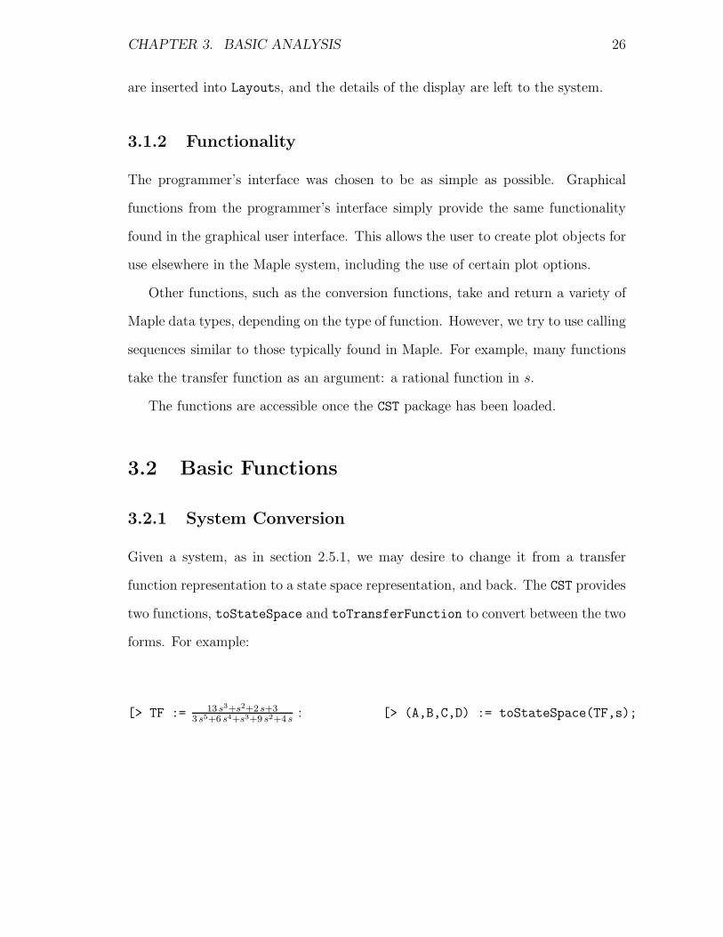
3.1.2 Functionality
The programmer’s interface was chosen to be as simple as possible. Graphical
functions from the programmer’s interface simply provide the same functionality
found in the graphical user interface. This allows the user to create plot objects for
use elsewhere in the Maple system, including the use of certain plot options.
Other functions, such as the conversion functions, take and return a variety of
Maple data types, depending on the type of function. However, we try to use calling
sequences similar to those typically found in Maple. For example, many functions
take the transfer function as an argument: a rational function in s.
The functions are accessible once the CST package has been loaded.
3.2 Basic Functions
3.2.1 System Conversion
Given a system, as in section 2.5.1, we may desire to change it from a transfer
function representation to a state space representation, and back. The CST provides
two functions, toStateSpace and toTransferFunction to convert between the two
forms. For example:
[> TF := 13 s3+s2+2 s+33 s5+6 s4+s3+9 s2+4 s
: [> (A,B,C,D) := toStateSpace(TF,s);

CHAPTER 3. BASIC ANALYSIS 27
−2−13
−3−43
0
1 0 0 0 00 1 0 0 00 0 1 0 00 0 0 1 0
,
[
10000
]
,
[ 13
133
23
1 0 ], 0
and back...
[> toTransferFunction(A, B, C,
D, s);
s+ 13
3s2+ 2
3s3+ 1
3s4
s5+2 s4+ 1
3s3+3 s2+ 4
3s
Note that the final transfer function is the normalized form of the original
transfer function.
3.2.2 Observability and Controllability
Given a multiple-state system in state-space form, it may be desired to know which
states are observable or controllable. Observability is the property that indicates
that each state of the system is observable from the output, that is, that the value
of each state may be deduced. Controllability is the property that indicates that
each state is controllable, that is, that each state may be affected by the input.
Given a state space system A, B, C, D of order n, we construct the observ-
ability matrix below:[
CT AT CT ... (AT )nCT
]
(3.1)
If the observability matrix is nonsingular, the system is observable.
Given the same system, the controllability matrix can be built in a similar way.
[
B AB A2B ... AnB
]
(3.2)
If this matrix is nonsingular, the system is controllable.

CHAPTER 3. BASIC ANALYSIS 28
Examples are given below for the 2nd order system
x = [ 1 00 2 ]x + [ 1
2 ]u, (3.3)
y = [ 1 0 ]x.
[> isControllable( [ 1 00 2 ], [ 1
2 ] );
true
[> isObservable( [ 1 00 2 ], [ 1 0 ] );
false
It can be easily seen that x1, x2 may both be modified by appropriate choices of
u1, u2, so the system is intuitively controllable. It can also be seen that y = x1, and
that x2 does not affect x1, so the system is not completely observable. In particular,
we say that x2 is not observable.
3.2.3 Hurwitz Test
Another commonly used test used on differential systems is the Hurwitz test for
polynomials. The Hurwitz test allows one to quickly check whether a system is
stable without explicitly computing the poles of the characteristic polynomial of
the system.
A method to compute this is provided in the Maple library, in the function
PolynomialTools:-Hurwitz. However, a method in Shinners [12] seems to give
better performance for the type of transfer function systems we are concerned with
in this thesis. Shinners presents a turn of the century method from Routh [11],
which computes the same result as the Maple function, but uses a different, faster
method.
CHAPTER 3. BASIC ANALYSIS 29
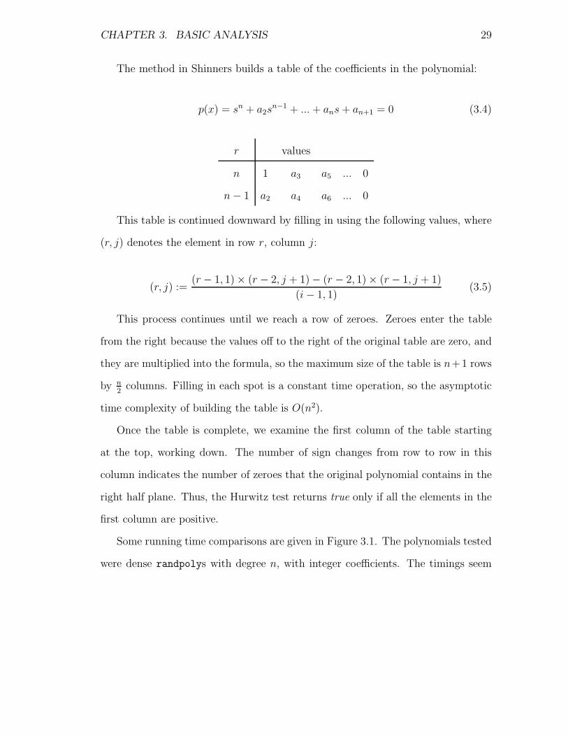
The method in Shinners builds a table of the coefficients in the polynomial:
p(x) = sn + a2sn−1 + ... + ans + an+1 = 0 (3.4)
r values
n 1 a3 a5 ... 0
n − 1 a2 a4 a6 ... 0
This table is continued downward by filling in using the following values, where
(r, j) denotes the element in row r, column j:
(r, j) :=(r − 1, 1) × (r − 2, j + 1) − (r − 2, 1) × (r − 1, j + 1)
(i − 1, 1)(3.5)
This process continues until we reach a row of zeroes. Zeroes enter the table
from the right because the values off to the right of the original table are zero, and
they are multiplied into the formula, so the maximum size of the table is n+1 rows
by n2
columns. Filling in each spot is a constant time operation, so the asymptotic
time complexity of building the table is O(n2).
Once the table is complete, we examine the first column of the table starting
at the top, working down. The number of sign changes from row to row in this
column indicates the number of zeroes that the original polynomial contains in the
right half plane. Thus, the Hurwitz test returns true only if all the elements in the
first column are positive.
Some running time comparisons are given in Figure 3.1. The polynomials tested
were dense randpolys with degree n, with integer coefficients. The timings seem

CHAPTER 3. BASIC ANALYSIS 30
to agree with the expected quadratic performance.
0 5 10 15 20 25 300
0.1
0.2Hurwitz Tests
PolynomialTools
Routh−Hurwitz
N
Tim
e (
sec)
Figure 3.1: Timing results of two Hurwitz algorithms.
The figure shows that the Routh-Hurwitz method described in Shinners is con-
siderably faster, especially on the small polynomials common in control system
design.
Elementary examples are given below.
[> RouthHurwitz( 1(s+1)3
, s, output=table );
true, 0,
1 3
3 1
83
0
1 0

CHAPTER 3. BASIC ANALYSIS 31
[> RouthHurwitz( 1(s+1)2(s+3)2(s−1)
, s, output=table );
true, 0,
1 14 −15
7 2 −9
967
−967
0
9 −9 0
ǫ 0 0
−9 0 0
In the second example, ǫ is a small positive number, filling in for a 0. This is
necessary to avoid a 0 in the left column. When determining the sign changes in
the left column, a limit as ǫ → 0 is taken to find the sign of the expression. Note
that ǫ may be involved in larger expressions as the matrix size gets larger and the
ǫ is propagated down, resulting in a more complicated expression to work with and
making it more difficult to find a limit.
As seen above, the CST software optionally returns the table used for inspection
by the user. This is particularly useful if free variables are utilized in the Hurwitz
analysis. For example, a common control problem is to select a gain K that provides
a fast system response, without resulting in an unstable system. This means we
must find the largest stable value of K. For example, if our characteristic equation
is a(s) = s3 + s2 + s + K, we have the output below:
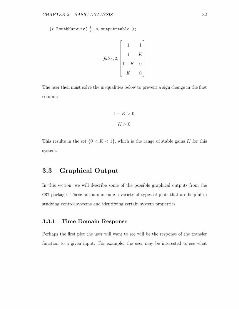
CHAPTER 3. BASIC ANALYSIS 32
[> RouthHurwitz( 1a
, s, output=table );
false, 2,
1 1
1 K
1 − K 0
K 0
The user then must solve the inequalities below to prevent a sign change in the first
column:
1 − K > 0,
K > 0.
This results in the set 0 < K < 1, which is the range of stable gains K for this
system.
3.3 Graphical Output
In this section, we will describe some of the possible graphical outputs from the
CST package. These outputs include a variety of types of plots that are helpful in
studying control systems and identifying certain system properties.
3.3.1 Time Domain Response
Perhaps the first plot the user will want to see will be the response of the transfer
function to a given input. For example, the user may be interested to see what

CHAPTER 3. BASIC ANALYSIS 33
happens when the system input is switched from 0 to 1. This plot is called the time
domain response of the transfer function.
This is actually a series of possible plot outputs. There are three input functions
that are commonly used when testing a system: the impulse, the step, and the ramp
inputs. These three input functions available in this category are outlined in Table
3.1.
Impulse Response r(t) =
1 when t = 0
0 for t > 0
Step Response r(t) =
0 when t = 0
1 for t > 0
Ramp Response r(t) =
0 when t = 0
t for t > 0
Table 3.1: Possible inputs for system response.
[> CST:-StepPlot( 1s2+2s+1
, s); [> CST:-RampPlot( 1s2+ 1
5s+1
, s);
Step Response
0
0.2
0.4
0.6
0.8
1
2 4 6 8 10
t
Ramp Response
0
2
4
6
8
10
2 4 6 8 10
t
Figure 3.2: Possible uses of the plotting functionality.

CHAPTER 3. BASIC ANALYSIS 34
A pair of example output plots is visible in Figure 3.2. The plot on the left
shows the response of a critically damped 2nd order system to a step input. The
input r(t) can be seen as the straight line across the top of the figure, and the
system output can be seen arcing to converge with the input. The system is called
critically damped because there is no overshoot, or oscillation, with the minimal
amount of damping. The plot on the right shows a system with a moderate amount
of overshoot that is responding to a ramp input. This system may, for example,
represent the position of a wobbly elevator ascending through time.
3.3.2 Root Locus
The root locus plot allows the user to view all the possible roots of the characteristic
equation of a system with respect to a positive free variable, K. This is equivalent
to viewing the possible eigenvalues of the system with a variety of possible gain
values. This is important to the engineer because often the gain is an easily tuned
value.
The corresponding command has been implemented in the function RootLocus.
This function takes a transfer function as an argument, which is a rational function,
with one or more of the coefficients dependent on K.
Given a transfer function N(s)D(s)
, the routine simply picks a variety of values for
K, plugs each into D(s), and solves D(s) = 0. The result, a constant in C, is then
plotted on the complex axis.
Some example root loci are visible in Figure 3.3. The figure on the left shows
the root locus of the critically damped second order system. The locus is quite

CHAPTER 3. BASIC ANALYSIS 35
simple, the roots are either on the real axis, symmetric around −1 + 0i, or are a
pair of complex roots above and below −1 + 0i.
The figure on the right in Figure 3.3 shows the root locus of a more complex third
order system. Using Hurwitz analysis, it may be seen that this system becomes
unstable when K > 2. So we can say that the two symmetric curved loci cross the
imaginary axis when K = 2. We can use the graphical information provided by the
plot to gain insight into expected system behavior for other values of K.
[> CST:-RootLocus( Ks2+s+K
); [> CST:-RootLocus( Ks3+s2+2s+K
);
Root Locus
–3
–2
–1
0
1
2
3
Imaginary
–2 –1.5 –1 –0.5
Real
Root Locus
–2
–1
0
1
2
Imaginary
–2 –1.5 –1 –0.5 0.5
Real
Figure 3.3: Possible uses of the root locus functionality.
Viewing the root locus diagram allows the user to determine which values of K
lead to desired system characteristics. For example, roots close to the imaginary
axis will lead to oscillatory performance. By experimenting with the root locus
diagram, the user may gain insight as to which roots are responsible for various
system behaviors.

CHAPTER 3. BASIC ANALYSIS 36
3.3.3 Nyquist Diagram
The Nyquist diagram is a commonly used tool that can also be used to determine
the system stability of a given transfer function. It uses a plot in the complex plane
to show the user where the roots of the characteristic polynomial are, and thus
whether the system is stable.
This plotting tool uses a mapping of the entire imaginary axis through the
transfer function and back onto the complex plane. So for the transfer function F ,
and i =√−1, we can think of this as the set of points:
±F (ωi), ω = 0...∞. (3.6)
This is a difficult plot to draw because as ω → ∞, F (ωi) will often converge,
connecting to the negative side of the plot for a proper rational function. There is
no easy place to truncate this expression, so we take a limit:
limω→∞
F (ωi) = Ω. (3.7)
Then we can start plotting points, starting from a small ω. At each step, we
compare our current location with the location of Ω, until we are close enough to
connect them. This gives a smooth-looking graph. We call the maximum allowable
distance between two plotted points the tolerance of the plot. If the tolerance is
too high, the plot appears rough, and so the user will be unable to observe some
important characteristics.
However, because of the large changes in scale of numbers used, an adaptive

CHAPTER 3. BASIC ANALYSIS 37
plotter is necessary. For example, for the simple transfer function
F (s) =1
s2 + 2s + 1, as ω → ∞, F (ωi) → 0. (3.8)
To capture this Nyquist diagram, we take the limit of F as ω → ∞, then plot F
until we are close enough to the limit 0 for a good image. As ω gets large, we have
to use a larger step in between to advance quickly, but without using a step larger
than the tolerance. The adaptive plotter is designed to do this. Some example
Nyquist diagrams are visible in Figure 3.4.
[> CST:-Nyquist( 1s2+2s+1
, s); [> CST:-Nyquist( 1s2+ 1
5s+1
, s);
Nyquist
–0.6
–0.4
–0.2
0
0.2
0.4
0.6
0.2 0.4 0.6 0.8 1
Nyquist
–4
–2
2
4
–2 –1 1 2
Figure 3.4: Possible uses of the Nyquist functionality.
It is interesting to note that the image on the left was computed with 268
function evaluations, while the function on the right took 1809 function evaluations.
This is indicative of the slow convergence of the transfer function on the right.

CHAPTER 3. BASIC ANALYSIS 38
3.3.4 Bode Diagram
The Bode diagram is another helpful tool when analyzing systems, and is similar
to the Nyquist plot, providing similar information. The diagram actually consists
of a pair of plots. For a transfer function F , the first plot contains values of |F (ω)|,
where ω starts at 0 and extends up along the imaginary axis. This first plot is
labelled the dB plot. The second plot contains the values of the phase of F (ω), in
degrees, for the same values of ω, and labelled the degrees plot.
Some example Bode diagrams are visible in Figure 3.5. The figures on the left
display the critically damped second order system. The figures on the right show
the second order system with a much smaller damping coefficient, leading to a spike
near ω = 1 in the dB plot, and a steeper drop in the degrees plot, both of which
are expected behavior.

CHAPTER 3. BASIC ANALYSIS 39
[> CST:-Bode( 1s2+2s+1
, s); [> CST:-Bode( 1s2+ 1
5s+1
, s);
Bode (DB)
–160
–140
–120
–100
–80
–60
–40
–20
0
dB
.1e–1 .1 1. .1e2 .1e3 .1e4 .1e5
Frequency
Bode (DB)
–160
–140
–120
–100
–80
–60
–40
–20
0
dB
.1e–1 .1 1. .1e2 .1e3 .1e4 .1e5
Frequency
Bode (DEG)
180
200
220
240
260
280
300
320
340
360
Degrees
.1e–1 .1 1. .1e2 .1e3 .1e4 .1e5
Frequency
Bode (DEG)
180
200
220
240
260
280
300
320
340
360
Degrees
.1e–1 .1 1. .1e2 .1e3 .1e4 .1e5
Frequency
Figure 3.5: Possible uses of the Bode diagram functionality.

Chapter 4
The Matrix Exponential
In the study of control systems, it is important to be able to predict the system
response to a variety of initial conditions. Given a complicated differential system,
the user may desire to compute the state of the system at various points in time
to study the response in terms of stability or convergence, or a variety of more
qualitative criteria. The state of the system may be expressed in closed form,
dependent on the time, t, using a computation called the matrix exponential. In this
chapter, we study various techniques to compute the matrix exponential efficiently
in a computer algebra system.
4.1 Definitions and Properties
For a given square matrix A, let
eAt = I + At +t2
2!A2 +
t3
3!A3 + ... =
∞∑
k=0
Aktk
k!(4.1)
40

CHAPTER 4. THE MATRIX EXPONENTIAL 41
where convergence is assumed. We may take the derivative of this function with
respect to t to obtain
(eAt)′ = A + A2t +t2
2!A3 +
t3
3!A4 + ...
= A
∞∑
k=0
Aktk
k!; (4.2)
= AeAt.
Thus we observe the most useful property of the matrix exponential: that the
system of linear differential equations
x(t) = Ax(t),
x(0) = x0,
is solved by
x(t) = eAtx0. (4.3)
The matrix exponential has certain important properties analogous to scalar
exponentials [2].
1. For scalars t0, t1, e(t0+t1)A = et0Aet1A.
2. For a scalar t, (etA)−1 = e−tA. This follows from (1).
3. For matrices A, B that are commutative by multiplication, eA+B = eAeB.
It is important to note that property 3 applies only to commutative matrices.

CHAPTER 4. THE MATRIX EXPONENTIAL 42
Consider our linearized system model, which relates the system state, x(t) and
the system input, u(t), to the derivative of the system state x(t), as in equation
(2.11):
x(t) = Ax(t) + Bu(t). (4.4)
We may use the properties of the matrix exponential to solve the system for x(t).
We first offer a solution analogous to the scalar case,
x(t) = eAtx0 + eAt
∫ t
0
e−AsBu(s)ds. (4.5)
By differentiating, factoring, and using property 1 we obtain:
x(t) = A(eAtx0 + etA
∫ t
0
e−sABu(s) ds) + Bu(t).
We observe that the sum in the parentheses is exactly our guess for the solution in
equation (4.5), so we may substitute:
x(t) = Ax(t) + Bu(t), (4.6)
proving our guess correct [2], and giving a closed form solution for x(t) in terms of
the matrix exponential, eAt.
Equation (4.5) shows that the system state, x(t), can be split into a sum of two
terms, one dependent on the initial state, and the other dependent on the input.
If u(t) = 0, we have equation (4.1) above. In this case, the matrix exponential is
referred to as the unforced response of the system to an initial state x0. Note also

CHAPTER 4. THE MATRIX EXPONENTIAL 43
that the second addend in (4.5) is independent of x0, meaning that this describes
the forced response of the system, unaffected by the initial state.
4.2 Computation
Adding up terms in a series is not the only way to evaluate the matrix exponential.
A variety of methods have been proposed, including methods based on the Cayley-
Hamilton theorem, matrix decomposition methods, and others. In this chapter
we will discuss methods to compute the exponential that are useful in an exact
arithmetic context.
Existing software to compute the matrix exponential is abundant. For example,
Matlab provides three different exponential algorithms that the user may select.
The command expm(A) or expm1(A) will compute the matrix exponential of A
using a method based on scaling and squaring and Pade approximation. Enter-
ing expm2(A) will compute the exponential via the Taylor series described above.
The third function, expm3(A) will perform the computation using eigenvectors and
eigenvalues, which is a matrix decomposition method discussed below.
Maple allows for the exact calculation of eAt with the use of the function
linalg[exponential]. This function and its methodology will be discussed below.
4.2.1 Polynomial Methods
Many polynomial methods derive from the Cayley-Hamilton theorem. This theo-
rem, originating independently from Cayley and Hamilton around 1860, shows that

CHAPTER 4. THE MATRIX EXPONENTIAL 44
every matrix satisfies its characteristic equation. That is, if
p(s) = det(sI − A) = sn + an−1sn−1 + ... + a0,
then p(A) = An + an−1An−1 + ... + I = 0.
If f(x) is a polynomial in x then we may compute the remainder of f and p,
f(x) = p(x)q(x) + r(x)
where the degree of r is less than n, the degree of p(x). This is also true for a power
series f(x), in which case q(x) is also a power series. Since p(A) = 0 we get that
f(A) = r(A).
Hence we need only find the n unknown coefficients for the remainder r(x).
Note that for any eigenvalue λ we have f(λ) = r(λ). Given n distinct eigenvalues
λ1...λn we may interpolate to obtain r(x) of degree n or less satisfying r(λi) = eλi .
In the case of a repeated eigenvalue λi of multiplicity k then p(x) = (x−λi)kp(x)
leaving
f(x) = (x − λi)kp(x)q(x) + r(x),
with deg(r(x)) < n. In this case we would have the k equations r(λ) = eλ, r′(λ) =
λeλ ... r(k−1)(λ) = λk−1eλ. Thus we still have n equations with n unknowns.
The Lagrange method for the matrix exponential is based on a direct interpo-
lation of the eigenvalues of A. It is effective if A has n different eigenvalues. In
this method, we build up the Lagrange terms and evaluate at A. We compute the

CHAPTER 4. THE MATRIX EXPONENTIAL 45
Lagrange terms using the form
Aj =n
∏
k=1,k 6=j
A − λkI
λj − λk. (4.7)
Then we add up the sum
etA =
n∑
j=1
eλjtAj. (4.8)
This results in an exact representation of the matrix exponential.
A similar method was proposed by Kirchner [6]. This technique works whether
or not A has repeated eigenvalues. In the case that A has n different eigenvalues,
the Kirchner method takes the form of equation (4.8). However, Kirchner does not
use the Lagrange terms to compute Aj . The first formula Kirchner gives for Aj is
pj(s) =
n∏
k=1,k 6=j
(s − λj)mj ; (4.9)
q(s) =n
∑
k=1
pk(s); (4.10)
Aj = q(A)−1pj(A). (4.11)
This method is clearly more expensive in terms of matrix operations because a
matrix polynomial must be evaluated and inverted. However, Kirchner gives an-
other method for computing Aj based on a Vandermonde matrix of the eigenvalues.

CHAPTER 4. THE MATRIX EXPONENTIAL 46
He computes
C =
1 1 ... 1
λ1 λ2 ... λn
......
...
λn−11 λn−1
2 ... λn−1n
−1
, (4.12)
Aj =n
∑
k=1
CkjAj−1. (4.13)
This method is easily seen to be similar to a Vandermonde interpolation of the
eigenvalues. An earlier method developed by Putzer [10] uses the Vandermonde
matrix implicitly in the context of solving a set of linear equations to satisfy initial
conditions of a linear differential equation. This method must solve an nth order
linear ODE, z(t), to build up the coefficients qj(t) of the polynomial
eAt =
n−1∑
j=0
qj(t)Aj. (4.14)
To solve the ODE z(t), we must compute the roots of the nth order polynomial,
then solve for the constants ki using t = 0:
1 1 ... 1
λ1 λ2 ... λn
......
...
λn−11 λn−1
2 ... λn−1n
k1
k2
...
kn
=
0
...
0
1
. (4.15)
However, because of the special right hand side in this equation, the solution

CHAPTER 4. THE MATRIX EXPONENTIAL 47
may be easily found. The ODE solution, z(t), is then used to compute the qj(t),
each of which is a linear combination of the exponentials, eλit. The solution is then
computed as above in equation (4.14).
Another Vandermonde-based procedure was used by Fulmer [5] that is function-
ally similar to the Putzer method, but based on the solutions to the initial value
problem
p(d
dt)(G(t)) = 0, G(0) = I, G′(0) = A, G(2)(0) = A2... (4.16)
Since dk
dtk(eAt) = AkeAt, G(t) = eAt. The general solution of the differential
equation, if we have n different eigenvalues, is
eAt = C1eλ1t + ... + Cne
λnt. (4.17)
We solve for the unknown matrices Ci by inverting a Vandermonde matrix of
the eigenvalues.
The current Maple implementation of the matrix exponential mentioned earlier
also uses a method based on interpolating the values of eλi at the eigenvalues,
λi. This method efficiently computes the coefficients of the Newton form of the
interpolating polynomial, resulting in a Horner-like polynomial in A. The method
plugs A into that expression, resulting in the exponential, eAt.
Limitations
Assume we have a matrix exponential eAt where A is a square matrix that contains
n2 exact entries. To compute the exact form of the matrix exponential, all polyno-

CHAPTER 4. THE MATRIX EXPONENTIAL 48
mial methods must compute the eigenvalues of A. This involves finding the roots
of the characteristic equation of A, which has coefficients that are polynomial in
the entries of A. If the degree of the characteristic equation is less than 4, the exact
roots may be found quite easily. If the degree is 5 or greater, finding the roots ex-
actly may be impossible, forcing the method to work with symbolic representations
of the actual roots. This greatly adds to the size of the expressions produced in the
output.
In addition, polynomial methods for the matrix exponential typically build up
a degree n polynomial in A with exponential coefficients which must represent the
matrix exponential. This polynomial is evaluated, giving the result in time O(n4).
This running time does not include the cost of the size of the expressions involved,
which is considerable given the multiplication of the aforementioned exponential
coefficients.
4.2.2 Matrix Decomposition Methods
Certain matrices have a non-zero structure that allows for an easier computation
of the matrix exponential. It will be shown that a variety of these structures may
be used to compute the matrix exponential efficiently.
For example, a n × n diagonal matrix D = diag(d1, ..., dn) may be exponenti-
ated with time complexity O(n), by simply exponentiating each element along the
diagonal, i.e. eDt = diag(ed1t, ..., ednt).
Another example of an easy matrix exponential is a Jordan block. A m × m

CHAPTER 4. THE MATRIX EXPONENTIAL 49
Jordan block may be exponentiated into a Toeplitz block:
Jλ =
λ 1 0 ... ... 0
0 λ 1 0 ... 0
.... . .
. . ....
0 0 ... 0 λ 1
0 0 ... ... 0 λ
, eJt =
eλt teλt t2
2!eλt ... ... tm
m!eλt
0 eλt teλt ......
.... . .
...
0 0 ... 0 eλt teλt
0 0 ... ... 0 eλt
. (4.18)
This calculation would take O(n) time, because the output is a Toeplitz matrix.
Triangular matrices are also relatively easy to exponentiate, using the recurrence
method given by Parlett [9]. Parlett’s method runs in time O(n3) and works on
triangular or block triangular matrices.
The existance of easy matrix exponentials allow us to compute exponentials of
matrices that are similar to a easy exponentials. Suppose we wish to compute the
exponential eAt where we have a matrix decomposition A = S−1PS, with ePt easy
to compute. Because of the power series definition of eAt,
eAt = I + S−1PSt +t2
2!S−1PSS−1PS +
t3
3!S−1PSS−1PSS−1PS... (4.19)
= S−1(I + Pt + P 2 t2
2!+ P 3 t3
3!...)S (4.20)
= S−1ePtS, (4.21)
giving us a matrix decomposition method to compute the matrix exponential.
A natural similarity decomposition to use is the Jordan form. This is the de-
composition A = Q−1JQ, where J is block diagonal, with each block in the form

CHAPTER 4. THE MATRIX EXPONENTIAL 50
(4.18). In exact arithmetic, the Jordan form may be computed with confidence, as
opposed to floating point arithmetic, where nearby eigenvalues may or may not be
equal.
If the Schur form of a matrix is given, we have A = Q−1TQ where Q is unitary
and T is upper triangular. Parlett’s method may be used to apply the exponential
function.
Limitations
These methods have the same difficulty that the polynomial methods suffer: the
exact eigenvalues must be computed, and are found as roots of an nth-degree poly-
nomial equation. An additional difficulty is that the similarity matrix must be
inverted. This is analagous to the computational difficulty of inverting the Vander-
monde matrix in the previous section for polynomial interpolation.
For example, benchmarking showed that the Jordan form method was 30% faster
than the current Maple method when n = 3, for matrices of random integers less
than 100. It was not competitive for n = 4, because the Jordan form (J, Q) could
not be computed in a reasonable amount of time, with A = Q−1JQ. This does
not include the time to invert Q. The current method, however, can exponentiate
a 4 × 4 matrix in a reasonable amount of time, and give a solution in terms of
RootOfs.

CHAPTER 4. THE MATRIX EXPONENTIAL 51
4.3 Special Cases
As discussed in the previous section, many matrices have exponentials that are easy
to compute. In this section we will describe a few of these cases and discuss their
computational complexity.
Matrices with one eigenvalue are an important case. If the matrix A has just
one eigenvalue, λ, then the exponential may be easily formed as given by Apostol
[3],
etA = eλtn−1∑
k=0
tk
k!(A − λI)k. (4.22)
This method uses a finite series because A−λI is a nilpotent matrix. Formulae
for some simpler matrices result from this method. For example, the exponential of
a triangular matrix where every nonzero entry is equal to x is a triangular Toeplitz
matrix where the ith off-diagonal entries may be written
eλ
i−1∑
j=0
( i−2j−1 )
xjtj
j!. (4.23)
This formula describes an O(n2) method to compute the exponential, assuming
the factorials are reused.
Another simple matrix exponential is the triangular band matrix with equal
coefficients. Assume the matrix A is like the previous example, but A has only a
band of such non-zeroes that is k-wide, i.e. A(k+1)...n1 = 0. In this case, a similar

CHAPTER 4. THE MATRIX EXPONENTIAL 52
method results. If we define a function f
f1j = (A − λI)j1, (4.24)
fij =
j−1∑
h=j−k+1
f(i−1)h,
then we may express the matrix exponential of A as the triangular Toeplitz matrix
based on the set of elements
eAti = eλ
n∑
j=1
fijxjtj
j!. (4.25)
This recursive definition allows the fij to be computable in amortized constant
time, giving a total running time of O(n2).
The form of other matrix exponentials may be deduced following the method
of Ziebur [15]. This gives a formula for eAt in terms of specified nilpotent matrices
and projection matrices. Ziebur shows that the exponential can be broken down:
eAt =
k∑
i=1
mi−1∑
j=0
tj
j!eλitN j
i Pi, (4.26)
where N is nilpotent and P is a projection matrix. When there is just one eigen-
value, k = 1, and P1 = I, giving the form from Apostol above, in equation (4.22).
If k = n, we have n eigenvalues, giving the interpolation form above in equation
(4.8), because we have mi = 1, i = 1..n.

CHAPTER 4. THE MATRIX EXPONENTIAL 53
The matrices N, P are dependent on A:
A =k
∑
i=1
λiPi + Ni, (4.27)
so if we know something about the structure of A, we have a simple form for the
matrix exponential that may be exploited.

Chapter 5
Feedback Control
Thus far, we have only discussed the study of differential systems - plants - from
a rather aloof standpoint. We have discussed the basic mathematical properties
of such systems, described software to graphically display their properties, and
shown how to compute the time domain reponse of such systems with the matrix
exponential. In this chapter we discuss the construction of control systems, that is,
systems created to control the plant in order to meet certain design requirements.
We have described our system of interest as equation (2.11), repeated here for
reference:
x(t) = Ax(t) + Bu(t). (5.1)
We assume that the operators A and B are fixed, they make up the plant
that we wish to control. The system state, x(t), is shown in equation (4.5) to be
dependent on only the initial conditions and the plant operators. So for a given
initial condition, if we wish to modify the behavior of x(t), we must find an input
54

CHAPTER 5. FEEDBACK CONTROL 55
function, u(t), to adjust the behavior of x(t) to meet our specifications.
The specifications that may be chosen are as varied as the possible applications.
A very common specification is that the system be stable, that is, x(t) < ∞ for
t → ∞. In a previous chapter we stated that this depends on the eigenvalues of
A. However, by using the input u(t) appropriately, we may keep the system state
bounded without modifying A.
In order to use u(t), let us assign u(t) to be a function of the current system
state and the reference signal, r(t). The reference signal is the desired state of the
system, the state to which x(t) should converge over time. So we redefine u(t) as
u(t) = f(x(t), r(t)). (5.2)
To stay within the bounds of the LTI model, we will linearize f with respect to
the two functions x, r as
u(t) = Fx(t) + r(t), (5.3)
assuming r(t) is simply added in. Now by substituting for u(t) in equation (5.1),
we can show how the complete system has been modified by F :
x(t) = Ax(t) + B(Fx(t) + r(t)),
x(t) = (A + BF )x(t) + Br(t), (5.4)
after some algebraic rearrangement. It is now clear that the system dynamics
are dependent on (A + BF ), and that system stability and performance will be
dependent on this new operator.

CHAPTER 5. FEEDBACK CONTROL 56
It can be shown that as long as the pair (A, B) is controllable, the eigenvalues
of the new system may be assigned to any desired values [14]. This certainly allows
for a system to be stabilized or tuned in a variety of ways.
In this chapter, we will describe how F may be chosen to assign the system
eigenvalues to user-defined values. For the state space system used above, there is
a direct method, which works in the single or multiple output case; and there is
the shortcut, known as Ackermann’s formula for the single output case. We will
then discuss a similar operation for systems of transfer functions. We will then
demonstrate some optimal control techniques for eigenvalue placement.
5.1 Ackermann’s Method
In the case of a SISO state space system, a well-known formula exists to compute the
matrix F , due to Ackermann [1]. This method depends on the system controllability
matrix, and the desired characteristic polynomial. The controllability matrix, C
is discussed in Chapter 3 and is elementary to compute. Since we require (A, B)
to be controllable we may compute the inverse, C−1. The desired characteristic
polynomial, αD, is simply built from its roots, which are our desired eigenvalues.
With these tools, we may express Ackermann’s formula,
F = enC−1αD(A) (5.5)
where en is the n-vector [0, ..., 0, 1]T .
This formula was implemented in Maple and performs well in an exact arith-

CHAPTER 5. FEEDBACK CONTROL 57
metic context. Computationally, the inverse of the controllability matrix is expen-
sive if the some of the entries of C are symbols; the denominator of each entry of
C−1 is the determinant of C which gets large rather quickly.
The evaluation of αD(A), with αD an n-th degree polynomial, is an O(n4)
operation, not including the size of the expressions. As before, these expressions
will get large quickly if symbols are involved. Overall, however, this method is
practical for most basic problems that would regularly need to be computed.
5.2 Direct Method
The direct method for eigenvalue assignment is a polynomial method to build the
operator F which will set the eigenvalues of (A+BF ) to their desired values. This
method is designed for multi-input, multi-output (MIMO) systems.
To begin this, we first compute (A+BF ), where A ∈ Kn×n, B ∈ Kn×m are given
matrices of scalars in the field K and F is a m × n matrix of unknown symbols,
Fij . (A + BF ) then consists of elements that are linear combinations of the Fij .
We represent the eigenvalues of (A + BF ) as the solutions of the degree n
characteristic polynomial, αF (λ). The coefficients of αF (λ) may be expressed as
multivariate polynomials in the Fij, we will name them gn−1, ..., g0.
The desired eigenvalues may be used to form our desired characteristic poly-
nomial, αD. By equating the coefficients from the unknown polynomial and our
desired polynomial we derive a system of equations that must be solved for the Fij
to build our desired system:
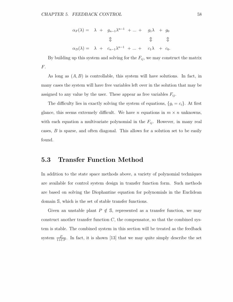
CHAPTER 5. FEEDBACK CONTROL 58
αF (λ) = λ + gn−1λn−1 + ... + g1λ + g0
m m m
αD(λ) = λ + cn−1λn−1 + ... + c1λ + c0.
By building up this system and solving for the Fij, we may construct the matrix
F .
As long as (A, B) is controllable, this system will have solutions. In fact, in
many cases the system will have free variables left over in the solution that may be
assigned to any value by the user. These appear as free variables Fij .
The difficulty lies in exactly solving the system of equations, gi = ci. At first
glance, this seems extremely difficult. We have n equations in m × n unknowns,
with each equation a multivariate polynomial in the Fij . However, in many real
cases, B is sparse, and often diagonal. This allows for a solution set to be easily
found.
5.3 Transfer Function Method
In addition to the state space methods above, a variety of polynomial techniques
are available for control system design in transfer function form. Such methods
are based on solving the Diophantine equation for polynomials in the Euclidean
domain S, which is the set of stable transfer functions.
Given an unstable plant P /∈ S, represented as a transfer function, we may
construct another transfer function C, the compensator, so that the combined sys-
tem is stable. The combined system in this section will be treated as the feedback
system P1+CP
. In fact, it is shown [13] that we may quite simply describe the set

CHAPTER 5. FEEDBACK CONTROL 59
of all such compensators using only simple polynomial arithmetic. If P = NP
DP, we
may pick X, Y so that
XNP + Y DP = 1.
With X and Y so chosen, we may describe the set of possible C that will stabilize
P as a set:
C ∈ S(P ) =
X + RDP
Y − RNP
. (5.6)
We may pick any transfer function R, as long as R ∈ S. This method allows us
great flexibility in picking a compensator. The downside is that, for a given R ∈ S,
we do not know what the properties of the system C or of the combined system
will be. So this method is much different from the previously described methods
that allow for the exact assignment of system eigenvalues. However, by treating
our transfer functions as elements of S, we may keep our compensator C ∈ S. The
ability to build stable compensators is beneficial for engineering reasons.
In order to ensure the stability of C, we first must show that P has the parity
interlacing property. A transfer function has this property if for each pair of pos-
itive zeroes of P , there are an even number of poles in between. This property is
necessary to find a function U that interpolates the values of DP (yi) at the positive
zeroes of NP (xi), and has no positive poles. Given U , we have the compensator
C = (U − DP )/NP .
Building the interpolant U is an n-step iterative process. Given the n pairs

CHAPTER 5. FEEDBACK CONTROL 60
(xi, yi), we start by setting U0 = yi. Then, we iterate over i:
f =i−1∏
j=1
s − xj
s + 1; (5.7)
b =( yi+1
U(xi+1))1/a − 1
f(xi+1), |b| <
1
||f || , a ∈ N; (5.8)
Ui+1 = (1 + bf)aUi. (5.9)
So the next Ui may always be constructed in terms of two positive integers a, b,
which must satisfy the constraint in the above inequality.
To satisfy this constraint, we must evaluate ||f || ∈ C+, with f a rational function
and the norm defined as:
||f || = sups∈C+
f(s). (5.10)
In general, this is very difficult or impossible to accomplish in exact arithmetic.
However, any pair a, b that satisfies the constraints will work. So we just need
to find a good floating point approximation of this value, then we can compare it
to b. It turns out that due to the maximum modulus theorem, the maximum is
guaranteed to be found along the imaginary axis. This allows us to use Maple to
easily compute a useful approximation, resulting in an exact solution for C.
Although the solution for C can be computed exactly by Maple in a reasonable
amount of time, the expressions involved get very large rather quickly. After the
algorithm was implemented, elementary tests on 3rd order systems, with length
near 50, resulted in output compensators of length over 700.

CHAPTER 5. FEEDBACK CONTROL 61
5.4 Eigenvector Control
Thus far, we have discussed how the most important properties of a linear system
may be modified by controlling the input so as to modify the eigenvalues of the
closed-loop system. These properties include the speed of the response of the system
to its input. In a SISO system, specifying the eigenvalues specifies the complete
system, so there is no room for modification, but in the MIMO case, the eigenvectors
may also be chosen to modify the shape of the response as well as the distribution
of the response of the system components.
An algorithm from Moore [8] allows the user to specify not only the eigenvalues,
but also the eigenvectors of the closed-loop system. The eigenvectors may be chosen
freely as long as they meet a few constraints: linear independence, consistency with
pairs of imaginary eigenvalues, and a third constraint that they must fall within a
specified subspace.
Given the system (5.1), and desired system eigenvalues and eigenvectors λi, vi,
Moore’s method desires to compute an m × n matrix F such that for i = 1..n,
(λiI − (A + BF ))vi = 0. (5.11)
The paper shows how matrix-vector multiplications and a single matrix inversion
may be used to compute the matrix F .
This method was implemented in Maple and works well for small systems, how-
ever, for more complex systems the n × n matrix inversion becomes more difficult
to perform.

Chapter 6
Conclusion
In this thesis, we have discussed a variety of control system concepts and algorithms.
We began by describing control systems from an abstract perspective, and then
described the mathematical model for such systems.
It is clear that such systems can be built up and expressed with computer
algebra, in fact, for transfer functions computer algebra is an ideal environment.
We have briefly shown how to perform certain elementary operations on control
systems and synthesis of control systems.
We also described a software package that meets the basic needs of an engineer
attempting to use computer algebra for control system computations. A highlight is
the Routh-Hurwitz computation which allows the user to determine system stability
exactly and efficiently. In addition, we demonstrated a package of plotting software
that allows the user to visualize many aspects of the control system in the Maple
system.
Another important tool in studying linear systems, the matrix exponential, was
62

CHAPTER 6. CONCLUSION 63
investigated and various methods for computing it were compared in a symbolic
context. We then showed how to perform a variety of eigenvalue and eigenvector as-
signment methods in exact arithmetic. With the implementation of these advanced
methods we found that symbolic analysis was beneficial for small or sparse systems,
but for larger systems expression swell quickly made the methods impossible to use.
In general, engineers can benefit from computer algebra analysis of control sys-
tems in the same way that scientific users benefit from computer algebra analysis
in general: the input and output is exact, free variables may be kept through a
computation, etc. In the case of feedback control, for example, a control system
could be computed using free variables, resulting in a feedback operator valid for a
whole class of systems. Using the rest of the given software, specific numbers could
be substituted in and further investigated to test a variety of operating conditions.
A complete model for the analysis of control systems symbolically, or with ex-
act arithmetic, is far from complete. Many of the inherent difficulties, such as
exact computation of eigenvalues or other linear algebra limitations are difficult
to work around. In this thesis, we have attempted to improve the control system
functionality in Maple while leaving these problems unsolved.
There are many further enhancements to Maple that would benefit control sys-
tem engineers. Some were overlooked in the CST package, such as the Nichols plot
and miscellaneous eigenvalue assignment techniques. Other topics are more com-
plex, such as algorithms to handle linear matrix equations and the algebraic Riccati
equations, which would benefit the study of optimal control.

Bibliography
[1] J. E. Ackermann. Der entwerf linearer regelungs systems in zustandstraum.
Regelungstech. Prozess-Datenverarb, 7, 1972.
[2] Panos J. Antsaklis and Anthony N. Michel. Linear Systems. McGraw-Hill,
1997.
[3] T. M. Apostol. Some explicit formulas for the matrix exponential etA. Amer-
ican Mathematical Monthly, 76, 1969.
[4] M. Chetty, K. P. Dabke, and B. Nath. Use of symbolic algebra toolbox in
system simulation and control. Melbourne VIC, November 2000. Matlab 2000.
[5] Edward P. Fulmer. Computation of the matrix exponential. American Math-
ematical Monthly, 82, 1975.
[6] R. B. Kirchner. An explicit formula for eAt. American Mathematical Monthly,
74, 1967.
[7] M. B. Monagan, K. O. Geddes, K. M. Heal, G. Labahn, S. M. Vorkoetter,
J. McCarron, and P. DeMarco. Maple 8 Introductory Programming Guide.
Waterloo Maple Inc., 2002.
64

BIBLIOGRAPHY 65
[8] B. C. Moore. On the flexibility offered by state feedback in multivariable
systems beyond closed loop eigenvalue assignment. IEEE Transactions on
Automatic Control, 21, 1976.
[9] B. N. Parlett. A recurrence among the elements of functions of triangular
matrices. Linear Algebra and its Applications, 14, 1976.
[10] E. J. Putzer. Avoiding the Jordan canonical form in the discussion of linear
systems with constant coefficients. American Mathematical Monthly, 73, 1966.
[11] E. Routh. Advanced Dynamics of a System of Rigid Bodies. Macmillan, 1905.
[12] Stanley M. Shinners. Modern Control System Theory and Design. John Wiley
Sons, Inc., 1998.
[13] M. Vidyasagar. Control System Synthesis: A Factorization Approach. The
MIT Press, Cambridge, Massachusetts, 1985.
[14] W. M. Wonham. On pole assignment in multi-input controllable linear systems.
IEEE Transactions on Automatic Control, 12, 1967.
[15] Allen D. Ziebur. On determining the structure of A by analyzing eAt. SIAM
Review, 12, 1970.

Appendix A
The CST Module
This appendix describes in more detail the Maple functions that were implemented
in the course of developing this thesis.
The state space system of interest is reprinted here for convenience.
x(t) = Ax(t) + Bu(t),
y(t) = Cx(t) + Du(t).
(A.1)
CST Package
• CST[toStateSpace] - convert a transfer function to a state space system
Calling sequence
toStateSpace(tf)
Parameters
tf - transfer function in s
66

APPENDIX A. THE CST MODULE 67
Description
– toStateSpace(tf) returns the state space system equivalent to the
given transfer function tf.
– The output is the sequence A,B,C,D representing the state space system
(A.1).
– As discussed in section 3.2.1.
• CST[toTransferFunction] - convert a state space system to a transfer
function
Calling sequence
toTransferFunction(A, B, C, D)
Parameters
A - n × n Matrix
B - n × m Matrix
C - m × n Matrix
D - m × m Matrix
Description
– toTransferFunction(A, B, C, D) returns the transfer function or trans-
fer function matrix equivalent to the system (A.1).
– The output is an nth degree rational function in s.
– As discussed in section 3.2.1.

APPENDIX A. THE CST MODULE 68
• CST[ImpulseResponse]
CST[StepResponse]
CST[RampResponse]
Calling sequences
ImpulseResponse(tf, options)
StepResponse(tf, options)
RampResponse(tf, options)
Parameters
tf - transfer function in s to be plotted
options - (optional) list of equations of form keyword = value
Description
– ImpulseResponse(tf) returns plot representing the response of the trans-
fer function system tf to the input u(0) = 1, u(t > 0) = 0.
– StepResponse(tf) returns plot representing the response of the transfer
function system tf to the input u(t >= 0) = 1.
– RampResponse(tf) returns plot representing the response of the transfer
function system tf to the input u(t >= 0) = t.
– As discussed in section 3.3.1.
• CST[ControllabilityMatrix]
CST[ObservabilityMatrix]
Calling sequences

APPENDIX A. THE CST MODULE 69
ControllabilityMatrix(A,B) ObservabilityMatrix(A,C)
Parameters
A - n × n Matrix
B - n × m Matrix
C - m × n Matrix
Description
– ControllabilityMatrix(A,B) returns the n × n controllability matrix
for the system (A.1).
– ObservabilityMatrix(A,C) returns the n × n observability matrix for
the system (A.1).
– As discussed in section 3.2.2.
• CST[isControllable]
CST[isObservable]
Calling sequences
isControllable(A, B)
isObservable(A, C)
Parameters
A - n × n Matrix
B - n × m Matrix
C - m × n Matrix
Description

APPENDIX A. THE CST MODULE 70
– IsControllable(A,B) returns a Boolean indicating whether or not the
system (A.1) would be controllable given A,B.
– IsObservable(A,C) returns a Boolean indicating whether or not the
system (A.1) would be observable given A,C.
– As discussed in section 3.2.2.
• CST[RootLocusPlot]
Calling sequences
RootLocusPlot(tf, options)
Parameters
tf - transfer function in s and K
options - (optional) list of equations of form keyword = value
Description
– RootLocusPlot(tf) returns a plot in the complex plane of the poles of
the transfer function tf for a range of values of K.
– The default range for values of K is 0..10, but may be modified by using
the argument Kvals = Kmin..Kmax, where Kmin, Kmax are numbers to
start and end the range of K.
– The argument view = [xmin..xmax, ymin..ymax] allows the user to
specify the region of the plane shown.
– As discussed in section 3.3.2.

APPENDIX A. THE CST MODULE 71
• CST[Nyquist]
Calling sequences
Nyquist(tf, options)
Parameters
tf - transfer function in s
options - (optional) list of equations of form keyword = value
Description
– Nyquist(tf) returns a plot in the complex plane containing the Nyquist
diagram of the transfer function tf.
– The argument view = [xmin..xmax, ymin..ymax] allows the user to
specify the region of the plane shown.
– As discussed in section 3.3.3.
• CST[Bode]
Calling sequences
Bode[type](tf, options)
Parameters
type - the type of Bode plot, DB or DEG
tf - transfer function in s
options - (optional) list of equations of form keyword = value
Description

APPENDIX A. THE CST MODULE 72
– BodePlot(tf) returns the Bode plot on the semilog axis of the transfer
function tf.
– The type specifier allows the user to create either the amplitude or
degrees plot by specifying the symbol DB or DEG.
– The argument view = [xmin..xmax, ymin..ymax] allows the user to
specify the region of the plane shown.
– As discussed in section 3.3.4.
• CST[FeedbackControl]
Calling sequences
FeedbackControl(A, B, eigs, options)
Parameters
A - n × n Matrix
B - n × m Matrix
eigs - n-Vector
options - (optional) list of equations of form keyword = value
Description
– FeedbackControl(A, B, eigs) returns an m × n Matrix F such that
Eigenvalues(A + B.F) = eigs. (A.2)
– The argument output = true returns any free variables as indexed sym-
bols f[i,j]. The default behavior is to set these variables to 0.

APPENDIX A. THE CST MODULE 73
– If m = 1 it is recommended to use CST[Ackermann].
– As discussed in section 5.2.
• CST[Ackermann]
Calling sequences
Ackermann(A, B, eigs)
Parameters
A - n × n Matrix
B - n-Vector
eigs - n-Vector
Description
– Ackermann(A, B, eigs) returns an n-row-Vector F to satisfy (A.2).
– As discussed in section 5.1.
• CST[StableCompensator]
Calling sequence
StableCompensator(P)
Parameters
P - rational function in s
Description
– StableCompensator(P) constructs a stable compensator C such that C,
as well as the closed-loop system, P
1+CP, are stable.

APPENDIX A. THE CST MODULE 74
– As discussed in section 5.3.
• CST[EigenvectorControl]
Calling sequences
EigenvectorControl(A, B, eigs, eigvs)
Parameters
A - n × n Matrix
B - n × m Matrix
eigs - n-Vector
eigvs - n-list of n-Vectors
Description
– EigenvectorControl(A, B, eigs, eigvs) returns an m×n Matrix F
such that:
Eigenvalues(A + B.F) = eigs and (A.3)
Eigenvectors(A + B.F) = eigvs. (A.4)
– As discussed in Chapter 5.
• CST[CSTI]
Calling sequences
CST[CSTI](tf)
Parameters
tf - (optional) rational function in s

APPENDIX A. THE CST MODULE 75
Description
– CSTI(tf) starts up the CSTI Maplet, which is a GUI that allows access
to many of the graphical tools in the CST. The argument tf, if present,
starts the Maplet with that function in the input box.
– As discussed in Chapter 3.

Appendix B
Vita
Justin Wozniak is a native of the state of Illinois in the USA. He graduated from St.
Edwards High School, Elgin, IL, in 1996. His undergraduate degree in Mathematics
and Computer Science with minors in Latin and Chemistry was awarded by the
University of Illinois at Urbana-Champaign in 2000. He currently lives and works
at the Hershey Montessori Farm School in Huntsburg, Ohio with his wife, Venus.
76