1

POLITECNICO DI TORINO

Master of Science in Mechatronic Engineering

Master of Science Thesis

SITO Control Approach to Autonomous Parking

Supervisor: Prof. Diego Regruto

Candidate:

Giuseppe Petralia

Academic Year 2018/2019

2

To my family,

the best part of me.

To my grandmother Maria,

the angel that protects me from above.

And to me,

that I never gave up.

3

“There is a driving force more powerful than

steam, electricity and nuclear power: the will.”

(A. Einstein)

“If you can dream it, you can do it”

(E. Ferrari)

4

INDEX

INTRODUCTION ............................................................................................................... 6

AUTONOMOUS DRIVING ............................................................................................... 8 1. HISTORY OF AUTONOMOUS DRIVING ..................................................................... 9

1.1 AUTONOMOUS DRIVING AND VEHICLES ........................................................... 11

1.1.1 AUTONOMOUS VEHICLES CAPABILITIES ...................................... 14

1.1.1.1 PERCEPTION .................................................................................................. 14 1.1.2 LOCALIZATION ..................................................................................... 19

1.1.3 PLANNING .............................................................................................. 20

1.1.3.1 AUTONOMOUS VEHICLE PLANNING SYSTEMS ................................... 20

1.1.3.2 MISSION PLANNING .................................................................................... 21

1.1.3.3 BEHAVIOURAL PLANNING ........................................................................ 21 1.1.3.4 MOTION PLANNING ..................................................................................... 22

1.1.3.5 COMBINATORIAL PLANNING ................................................................... 22

1.1.3.6 SAMPLING-BASED PLANNING .................................................................. 23

1.1.3.7 DECISION MAKING FOR OBSTACLE AVOIDANCE ............................... 24 1.1.3.8 PLANNING IN SPACE-TIME ........................................................................ 25

1.1.3.9 PLANNING SUBJECT TO DIFFERENTIAL CONSTRAINTS .................... 25

1.1.3.10 INCREMENTAL PLANNING AND REPLANNING .................................. 27

AUTONOMOUS PARKING ............................................................................................ 29 2. AUTONOMOUS PARKING EVOLUTION .................................................................. 30

2.1 DIRECT TRAJECTORY PLANNING: HUMAN-LIKE PARKING......... 32

2.2 INTELLEGENT AUTONOMOUS PARKING CONTROL SYSTEM ..... 38

2.2 FAST PARALLEL PARKING USING GOMPERTZ CURVES ............... 41 LATERAL DYNAMICS PROBLEM .............................................................................. 49

3. LATERAL DYNAMICS ANALYSYS........................................................................... 50

3.1 YAW STABILITY CONTROL SYSTEMS ............................................... 50

3.2 KINEMATIC MODEL OF LATERAL VEHICLE MOTION ..................................... 51 LINEARIZATION OF NONLINEAR SYSTEMS ......................................................... 60

4. FEEDBACK LINEARIZATION .................................................................. 61

4.1 CANONICAL FORM OF FEEDBACK LINEARIZATION ................................ 61

4.2 INPUT-STATE LINEARIZATION ....................................................................... 62

4.4 THE INTERNAL DYNAMICS OF LINEAR SYSTEM ...................................... 64 4.5 THE ZERO-DYNAMICS ...................................................................................... 65

5

4.6 INPUT-STATE LINEARIZATION OF SISO SYSTEMS .................................... 66

SYSTEM CONTROL DESIGN ....................................................................................... 69 5. TIME-STATE CONTROL FORM .................................................................................. 70

5.1 MATHEMATICAL ANALYSIS AND SIMULINK TSC DESIGN .......... 72

5.2 LINEAR PLANT MODEL AND CONTROL DESIGN ............................ 76

5.2.1 SINGLE INPUT TWO OUTPUT (SITO) SYSTEMS ........................................ 80 CONCLUSIONS ................................................................................................................ 87

LIST OF FIGURES ........................................................................................................... 88

BIBLIOGRAPHY .............................................................................................................. 91

6

INTRODUCTION Since the production of the first vehicles, the companies have always pushed themselves to

overcoming every limit and to the continuous research of perfection in terms of aesthetics,

safety, performance, drivability. In recent decades, however, with the advent of the new

generations with different mentalities and needs than those of the past, new objectives and

other frontiers have been added to overcome: to ensure that it is as autonomous as possible

and that it can gradually free the driver from the load driving, eliminating some of those

daily sources of stress, tension, fatigue while achieving a smoother and free-error driving

experience.

Within this context, the goal of the thesis is to preliminary analyse the autonomous driving

and vehicles and the related problems and then to face with the realization of one the main

studied ADAS (Advanced Driver Assistance Systems).

The first chapter highlights the evolution of the autonomous vehicles over the years. In

particular, it is explained the reasons that made the car-maker and vendors think about the

development of something with strong potential that could change drastically the next future

of the transport system and framework. The focus analysis of this section is to understand

how the autonomy concept within this context can put considerable contribution by upsetting

the human life. For this aim, evaluation of all pros and cons to 360 degrees was made taking

into account the autonomy levels reached and to be achieved in the coming years. The last,

but the main part of this first chapter is dedicated to a detailed analysis of the different

working principle of an autonomous vehicle in terms of electronic perception of each

elements of the surrounding environment and the different classes of planning.

Among the various autonomous driving systems that are taking hold in recent years, one of

the most important is that related to parking, the so-called park assist that allows the driver

to make a perfect parking trajectory in terms of safety and efficiency. Particularly, in the

second chapter it is presented an historical excursus on how this technology has evolved

starting from a purely sensor notice approach to a recent studied autonomous parking with a

multiple level control process.

For this reason, several literature approaches to this problem are listed and explained within

this part. Obviously, for each researcher contributions the mathematical aspects are pointed

out with a particular attention to the vehicle dynamics.

The main point of this thesis work was the autonomous parking realization in the

MATLAB/Simulink environment by means a 2-degrees of freedom multivariable feedback

7

control system based on control of two reference variable: lateral position in terms of

trajectory to follow, a typical parallel parking S-trajectory, and yaw angle of the vehicle both

generated by an appropriate external control, the Time State control discussed in the fifth

chapter. The aim of this double particular control is to realize a perfect parallel parking that

is one the three noted types of parking situations.

To obtain the desired results, a linear bicycle model is considered after a linearization of a

starting nonlinear model whose equations are derived in the third chapter. There exist a lot

of linearization methods, but the one discussed in the fourth chapter is the feedback

linearization which allows to have a more treatable model.

When one thinks about a parking situation, it important to consider the problem of the lateral

dynamics, subject of deep study within the thesis. Fundamentally, the control of the yaw

stability of a vehicle is treated and one derives that the bicycle model can well-approximates

the vehicle behaviour and dynamics under several assumptions.

The final linear bicycle model represents the plant of the system as a SITO system, a single

output (steering angle) and the two-output system to be controlled as it is possible to see in

the fifth and last chapter.

The overall final control is realized thanks to a combination of a TISO Control derived from

the Freudenberg and Middleton studies and several feedforward filters mathematically

calculated and design based on the matrix assumptions which ties the input and the output

of the entire system.

The base idea applied to obtain the optimal following of the refence inputs is to impose in a

cross way the sensitivity and complementary sensitivity behaviours to the transfer functions

involved within the system taking into account the stability of the same.

Finally, a series of consideration and remarks are made on the simulations which show the

obtained good and optimal results of the control scheme by means the Simulink scope graph.

The simulations are based on a comparison of the reference inputs of yaw angle and lateral

trajectory and the same derived output by also analysing the final steering angle.

8

CHAPTER 1

AUTONOMOUS DRIVING

9

AUTONOMOUS DRIVING 1. HISTORY OF AUTONOMOUS DRIVING The story of the driverless car begins in the USA in the 1920. Driver error was seen as being

a prime cause of accidents. First developments were done on the field of aviation and radio

engineering giving a perspective to obtain accident-free and self-driving automobiles.

In Paris, Lawrence B. Sperry introduced a gyroscope airplane stabilizer; a pilot assistant

climbed out onto the right wing during the flight, while the pilot stood up and raised his

hands above his head. The system automatically equilibrated the aircraft, even if it did not

fully relieve the pilot of steering wheel. Furthermore, engineers though that the radio

technology was one of the technical requirements needed to be able to create a self-driving

car. The new science of radio guidance was engaged with the remote control of moving

mechanisms by means of radio waves, a technology developed by the US military which

was experimenting with remote-controlled ships and aircraft.

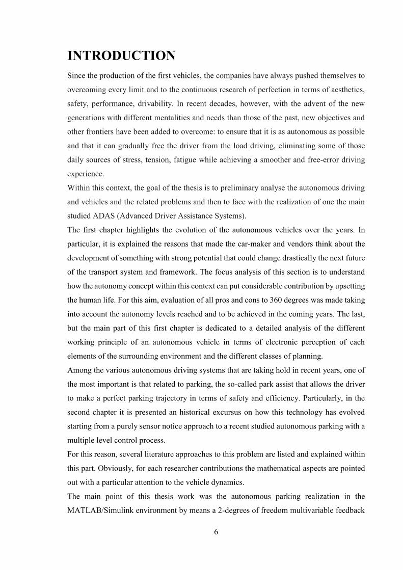
From 1930 to 1950 various appeared in

the public, where manipulate the brakes,

steering wheel and horn of vehicles

driving in front of another one was

possible, by using a spherical antenna that

received the code.

In the 1950s, the idea of remote-

controlled automobiles was abandoned

introducing a guide wire vision concept and in 1958 General Motor’s Center in Michigan

completed a test route of one mile.

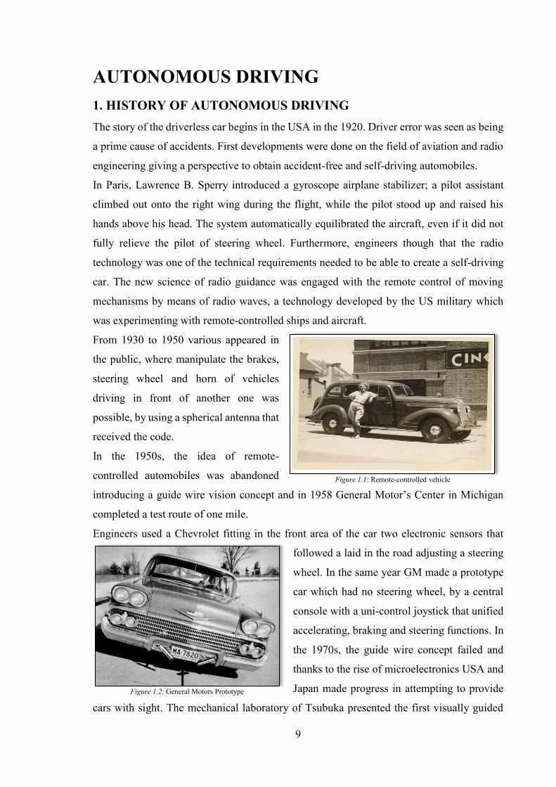
Engineers used a Chevrolet fitting in the front area of the car two electronic sensors that

followed a laid in the road adjusting a steering

wheel. In the same year GM made a prototype

car which had no steering wheel, by a central

console with a uni-control joystick that unified

accelerating, braking and steering functions. In

the 1970s, the guide wire concept failed and

thanks to the rise of microelectronics USA and

Japan made progress in attempting to provide

cars with sight. The mechanical laboratory of Tsubuka presented the first visually guided

Figure 1.1: Remote-controlled vehicle

Figure 1.2: General Motors Prototype

10

autonomous vehicle that could record and on-

board process pictures of lateral guide rails on

the via two cameras, with the car able to move

with a speed of 10 Km/h. The rise of

microelectronics led to an increasing use of

electronics in vehicle technology and the

launch of the first on-board computers in the series 7 BMW. The era of active driver-

assistance systems that directly intervene in the driving process began with the introduction

of ABS in 1978.

In the 1980s, the research on autonomous vehicles became a serious research topic for

academic and industrial research in many countries with the new concept of vision—based

autonomous driving. At first, the industry had expressed its preference for lateral guidance

of cars using electromagnetic fields generated by cables in the road, but then the Ernst

Dickmanns team from University of Munich successfully convinced the industry to privilege

the concept of machine vision that would allow the detection of obstacles and avoid

additional costs in infrastructure.

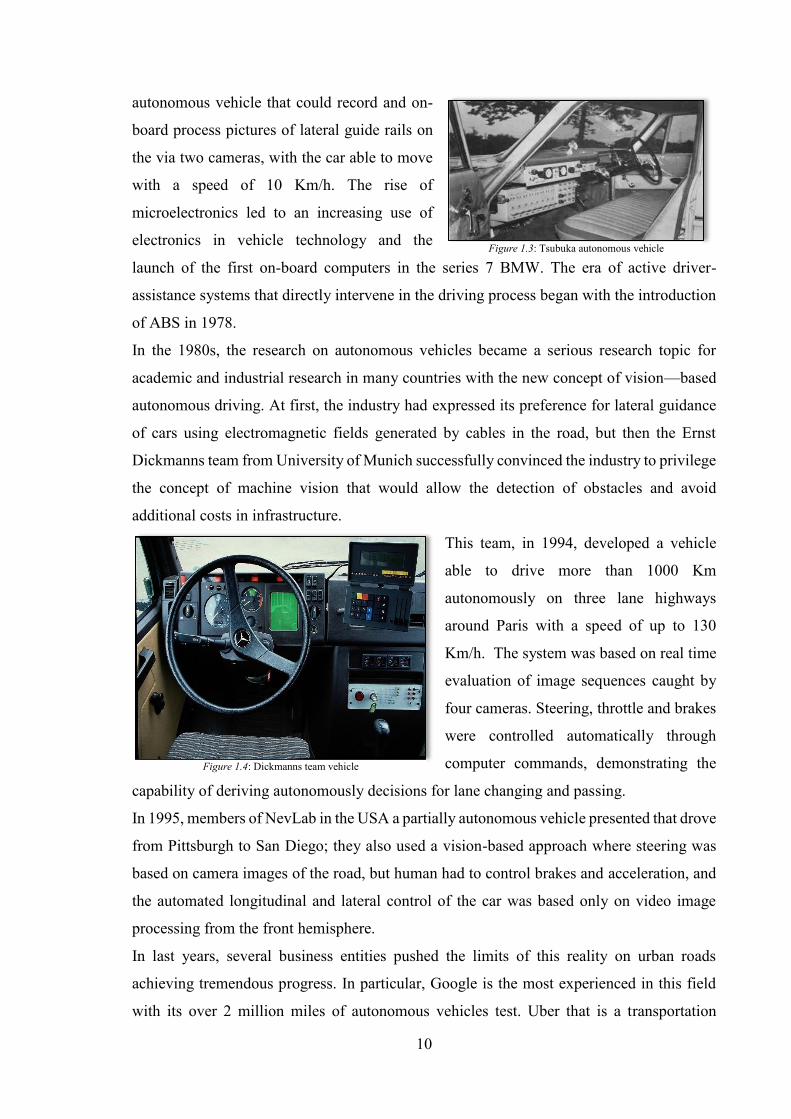
This team, in 1994, developed a vehicle

able to drive more than 1000 Km

autonomously on three lane highways

around Paris with a speed of up to 130

Km/h. The system was based on real time

evaluation of image sequences caught by

four cameras. Steering, throttle and brakes

were controlled automatically through

computer commands, demonstrating the

capability of deriving autonomously decisions for lane changing and passing.

In 1995, members of NevLab in the USA a partially autonomous vehicle presented that drove

from Pittsburgh to San Diego; they also used a vision-based approach where steering was

based on camera images of the road, but human had to control brakes and acceleration, and

the automated longitudinal and lateral control of the car was based only on video image

processing from the front hemisphere.

In last years, several business entities pushed the limits of this reality on urban roads

achieving tremendous progress. In particular, Google is the most experienced in this field

with its over 2 million miles of autonomous vehicles test. Uber that is a transportation

Figure 1.3: Tsubuka autonomous vehicle

Figure 1.4: Dickmanns team vehicle

11

network company would upset the taxi markets by introducing self-driving cars piloted

thanks to a program already underway which replaces all their human drivers. Instead Tesla

has already introduced an autopilot feature in their Model S cars in 2016.

Recently, researchers of ADAS (advanced driving autonomous system) has increased

enormously and most car companies are developing new solutions to make a fully

autonomous driving system trying to let the driver no safety checks. [1]

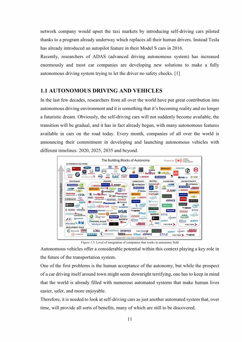
1.1 AUTONOMOUS DRIVING AND VEHICLES In the last few decades, researchers from all over the world have put great contribution into

autonomous driving environment and it is something that it’s becoming reality and no longer

a futuristic dream. Obviously, the self-driving cars will not suddenly become available, the

transition will be gradual, and it has in fact already begun, with many autonomous features

available in cars on the road today. Every month, companies of all over the world is

announcing their commitment in developing and launching autonomous vehicles with

different timelines: 2020, 2025, 2035 and beyond.

Autonomous vehicles offer a considerable potential within this context playing a key role in

the future of the transportation system.

One of the first problems is the human acceptance of the autonomy, but while the prospect

of a car driving itself around town might seem downright terrifying, one has to keep in mind

that the world is already filled with numerous automated systems that make human lives

easier, safer, and more enjoyable.

Therefore, it is needed to look at self-driving cars as just another automated system that, over

time, will provide all sorts of benefits, many of which are still to be discovered.

Figure 1.5: Level of integration of companies that works in autonomy field

12

Autonomous driving can definitely be scary to some, but it’s hard to deny the benefitsin

terms of additional safety, performance improvement, greater accessibility and increased

productivity. Furthermore, they surely have a positive impact on the environment thanks to

the capability to alleviate the road congestion and then improve the road efficiency. It would

also greatly improve the mobility of elderly and disabled people.

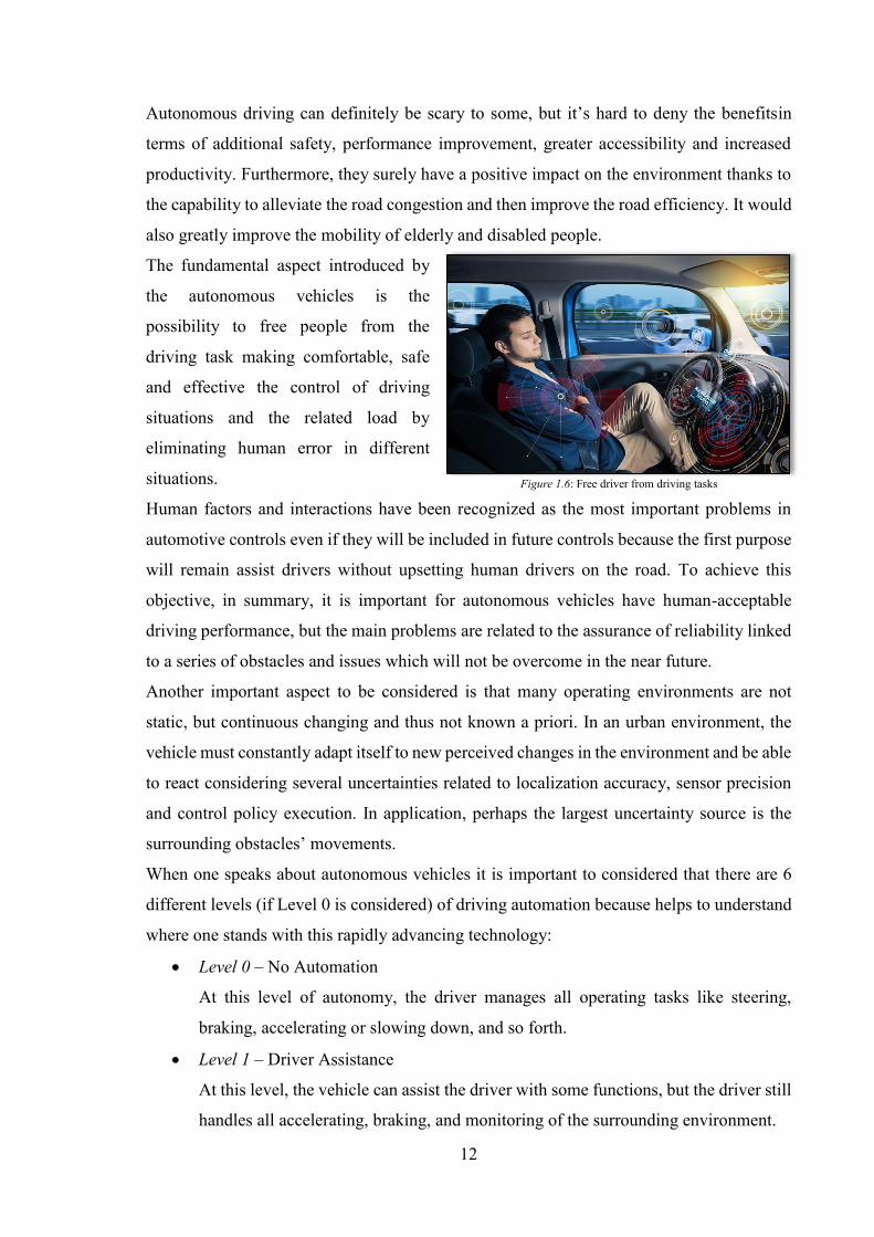
The fundamental aspect introduced by

the autonomous vehicles is the

possibility to free people from the

driving task making comfortable, safe

and effective the control of driving

situations and the related load by

eliminating human error in different

situations.

Human factors and interactions have been recognized as the most important problems in

automotive controls even if they will be included in future controls because the first purpose

will remain assist drivers without upsetting human drivers on the road. To achieve this

objective, in summary, it is important for autonomous vehicles have human-acceptable

driving performance, but the main problems are related to the assurance of reliability linked

to a series of obstacles and issues which will not be overcome in the near future.

Another important aspect to be considered is that many operating environments are not

static, but continuous changing and thus not known a priori. In an urban environment, the

vehicle must constantly adapt itself to new perceived changes in the environment and be able

to react considering several uncertainties related to localization accuracy, sensor precision

and control policy execution. In application, perhaps the largest uncertainty source is the

surrounding obstacles’ movements.

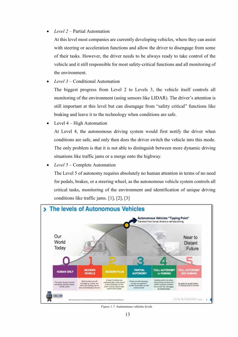
When one speaks about autonomous vehicles it is important to considered that there are 6

different levels (if Level 0 is considered) of driving automation because helps to understand

where one stands with this rapidly advancing technology:

• Level 0 – No Automation

At this level of autonomy, the driver manages all operating tasks like steering,

braking, accelerating or slowing down, and so forth.

• Level 1 – Driver Assistance

At this level, the vehicle can assist the driver with some functions, but the driver still

handles all accelerating, braking, and monitoring of the surrounding environment.

Figure 1.6: Free driver from driving tasks

13

• Level 2 – Partial Automation

At this level most companies are currently developing vehicles, where they can assist

with steering or acceleration functions and allow the driver to disengage from some

of their tasks. However, the driver needs to be always ready to take control of the

vehicle and it still responsible for most safety-critical functions and all monitoring of

the environment.

• Level 3 – Conditional Automation

The biggest progress from Level 2 to Levels 3, the vehicle itself controls all

monitoring of the environment (using sensors like LIDAR). The driver’s attention is

still important at this level but can disengage from “safety critical” functions like

braking and leave it to the technology when conditions are safe.

• Level 4 – High Automation

At Level 4, the autonomous driving system would first notify the driver when

conditions are safe, and only then does the driver switch the vehicle into this mode.

The only problem is that it is not able to distinguish between more dynamic driving

situations like traffic jams or a merge onto the highway.

• Level 5 – Complete Automation

The Level 5 of autonomy requires absolutely no human attention in terms of no need

for pedals, brakes, or a steering wheel, as the autonomous vehicle system controls all

critical tasks, monitoring of the environment and identification of unique driving

conditions like traffic jams. [1], [2], [3]

Figure 1.7: Autonomous vehicles levels

14

1.1.1 AUTONOMOUS VEHICLES CAPABILITIES The main capabilities of an autonomous vehicles software system can be categorized into

three categories:

• perception

• planning

• control

Also, the communications between two vehicles, Vehicle-to-Vehicle (V2V) can be exploited

to have improvement in the perception or planning areas also through the vehicle

cooperation.

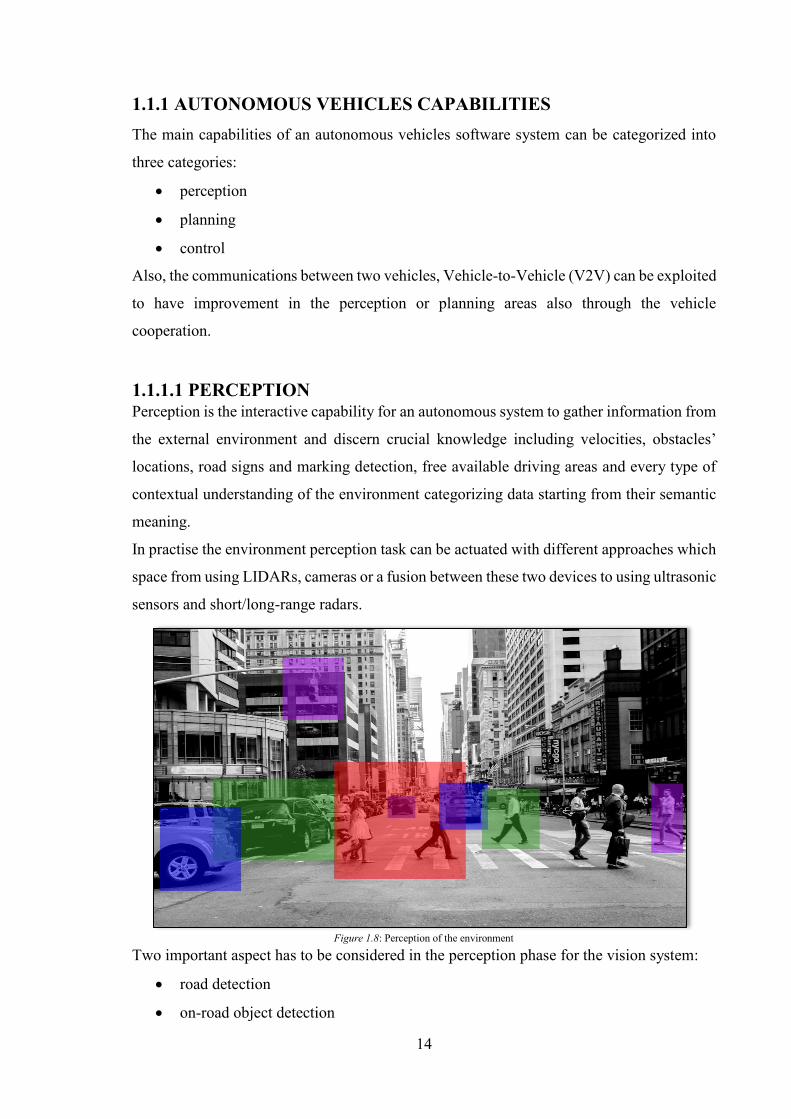
1.1.1.1 PERCEPTION Perception is the interactive capability for an autonomous system to gather information from

the external environment and discern crucial knowledge including velocities, obstacles’

locations, road signs and marking detection, free available driving areas and every type of

contextual understanding of the environment categorizing data starting from their semantic

meaning.

In practise the environment perception task can be actuated with different approaches which

space from using LIDARs, cameras or a fusion between these two devices to using ultrasonic

sensors and short/long-range radars.

Two important aspect has to be considered in the perception phase for the vision system:

• road detection

• on-road object detection

Figure 1.8: Perception of the environment

15

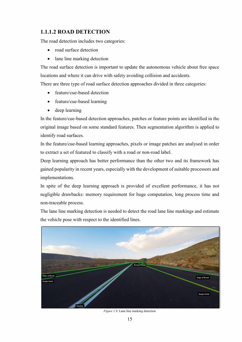
1.1.1.2 ROAD DETECTION The road detection includes two categories:

• road surface detection

• lane line marking detection

The road surface detection is important to update the autonomous vehicle about free space

locations and where it can drive with safety avoiding collision and accidents.

There are three type of road surface detection approaches divided in three categories:

• feature/cue-based detection

• feature/cue-based learning

• deep learning

In the feature/cue-based detection approaches, patches or feature points are identified in the

original image based on some standard features. Then segmentation algorithm is applied to

identify road surfaces.

In the feature/cue-based learning approaches, pixels or image patches are analysed in order

to extract a set of featured to classify with a road or non-road label.

Deep learning approach has better performance than the other two and its framework has

gained popularity in recent years, especially with the development of suitable processors and

implementations.

In spite of the deep learning approach is provided of excellent performance, it has not

negligible drawbacks: memory requirement for huge computation, long process time and

non-traceable process.

The lane line marking detection is needed to detect the road lane line markings and estimate

the vehicle pose with respect to the identified lines.

Figure 1.9: Lane line marking detection

16

The information obtained from this type of detection is useful for the vehicle control systems

even if it has remained as a challenging problem due to the fact that it has to cope with a

range of uncertainties related to road singularities and traffic road reality, which may include

variation of lighting conditions, consumed lane markings, and important markings such as

warning text, zebra crossings and directional arrows.

The lane line detection algorithms are generally 3-steps algorithms:

1. lane line feature extraction, to identify pixels of each lane line marking through

colour and edge detection and eliminate the non-lane marking pixels basing on the

fact that the lane markings have high contrast with respect to road pavement;

2. fitting the pixels into different high-level representations of the lane to obtain a model

(for example straight lines, zigzag line, parabolas, and hyperbolas);

3. estimating the vehicle pose based on the extracted model on the previous step.

It may exist a fourth step before the estimation of the vehicle pose to impose temporal

continuity, improve estimation accuracy and prevent detection failures.

Most approaches in the literature are based on the observations that lane markings have large

contrast compared to road pavement.

Finally, in the lane-level localization the vehicle lateral position and moving orientation are

estimated based on the lane line model.

1.1.1.3 ON-ROAD OBJECT DETECTION This type of detection mainly covers vehicle and pedestrian object classes and in particular

it is based on deep learning methods.

Despite the importance of this detection, it’s not enough for the autonomous vehicle

application because the methods are not robust due to different appearances, shapes, sizes

and types of objects.

1.1.1.4 LIDAR LIDAR (that stands for Laser Imaging Detection and Ranging or Light Detection and

Ranging) is a remote sensing technique that allows to determine the distance of an object or

a surface using millions of light pulses per second sent in a well-designed pattern. For most

of the autonomous vehicles which are research object LIDARs are the basis for object

detection, even if the cost of 3D LIDARs can be prohibitive to many applications.

In particular, with its rotating axis, LIDAR creates a dynamic 3D map of the environment.

17

The source of a LIDAR system is a laser, which is a coherent beam of light with precise

wavelength, sent to the system or the object to be observed and reflected back as sparse 3D

points representing and object’s surface location. The problem is that the reconstruction is

never perfect because generally there are missing points returned by the LIDAR and patterns

result unorganized.

There are three representations of the points generally used:

• point clouds

• features

• grids

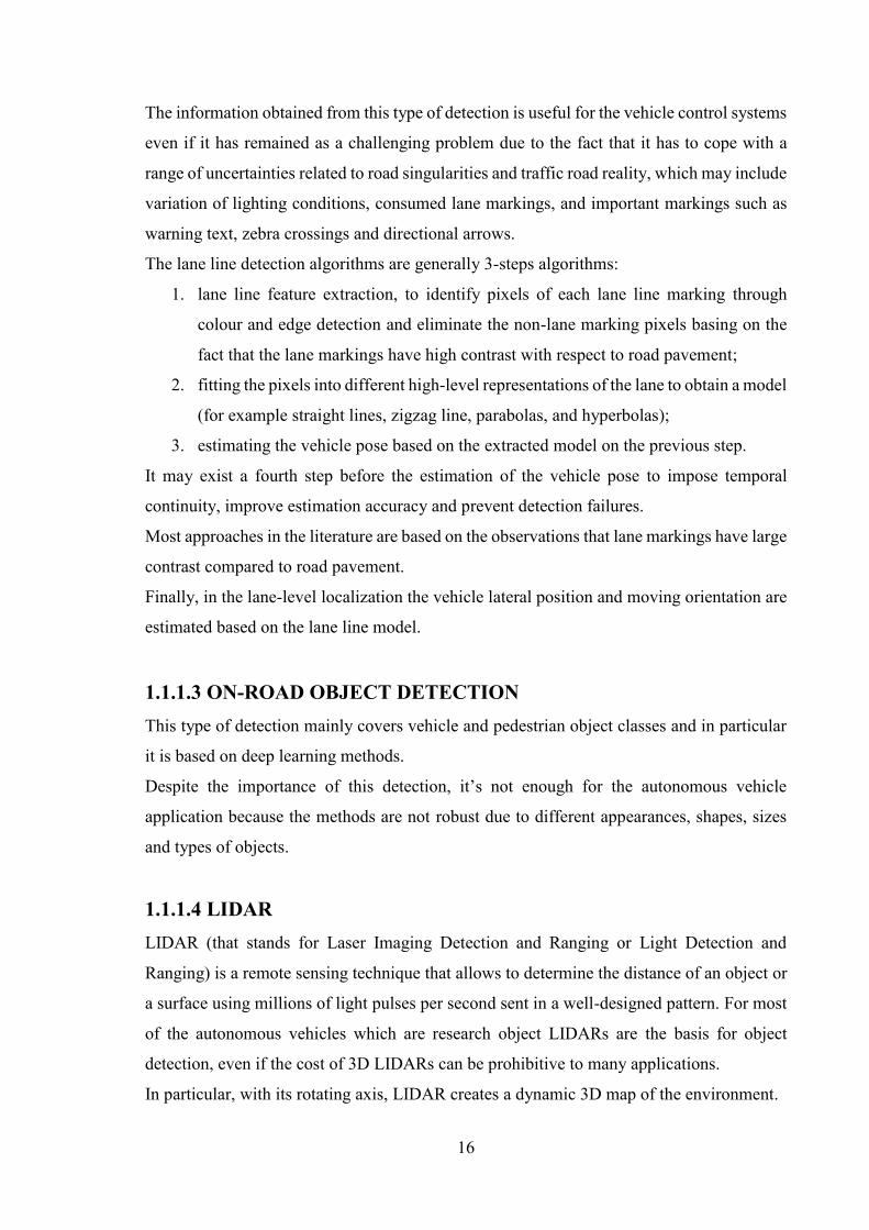
Point cloud-based approaches

provide a great environment

representation using raw sensor

data.

This approach is useful for further

processing but involve an increase

of processing time and a reduction

of the memory efficiency.

Feature based approaches represent the environment thanks to the parametric features (lines

and surfaces) extracted out of the point cloud. Even if this approach is too abstract, it’s the

most memory-efficient and accurate.

Grid based approaches discretize the space creating small grids full of information from the

point cloud in order to establish a neighborhood point.

Figure 1.10: LIDAR detection

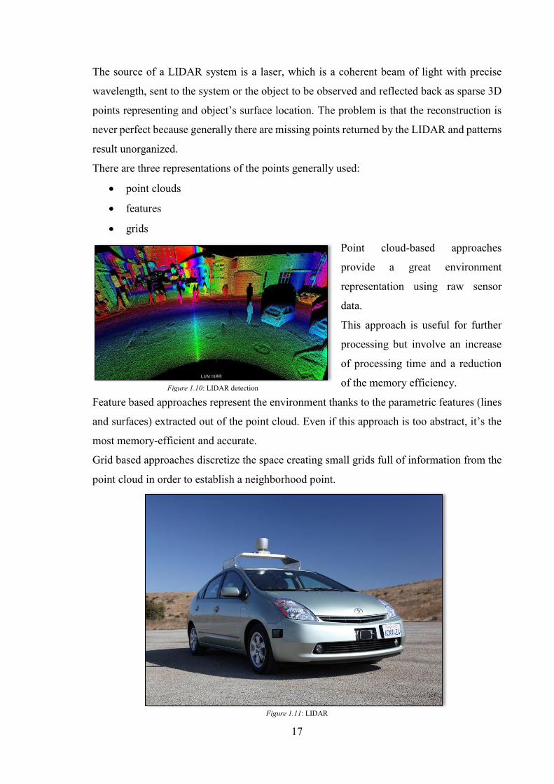
Figure 1.11: LIDAR

18

Generally, two procedures are needed to receive 3D point cloud information:

1. segmentation

2. classification

And non-mandatory third one, which is the time integration, that improve the consistency

and the accuracy of the two previous steps.

Segmentation refers to the important clustering process that gathers the points into multiple

homogeneous groups.

Classification is the process that recognizes the class and type of segmented clusters

(pedestrian, road surface, bike, car, etc.).

The algorithm for the segmentation can be part of five categories:

• edge based method

• region based method

• model based method

• attribute based method

• graph based method

Edge based methods are generally noise susceptible and they are adopted in tasks in which

the considered object has artificial edge features (for example curb survey). For this reason

this approach is not suitable for nature scene detection.

Region based methods through certain criteria (surface normal, Euclidean distance, etc.) use

particular region growing mechanism to cluster neighborhood points.

Model based methods are normally designed to segment the ground plane. They exploit

standard models in mathematic form like plane, cone, sphere, cylinder in order to fit the

points.

Attribute based methods are a 2-step approach in which for first the attribute is computed

for each point and later these points are clustered depending on the associated attributes.

Graph based methods insert the point cloud into a graph structure in which each point is a

vertex/node and the connections between near points are graph edges. This method is very

effective in image semantic segmentation.

After the segmentation process each cluster, that contains information from spatial

relationship to LIDAR intensity of the points, need to be assigned to an object category.

Generally, in order to make efficient the entire perception process a sensor fusion technique

is applied in order to exploit at maximum the advantages of each sensor.

A fusion between a LIDAR and a camera can be convenient because advantages of one are

19

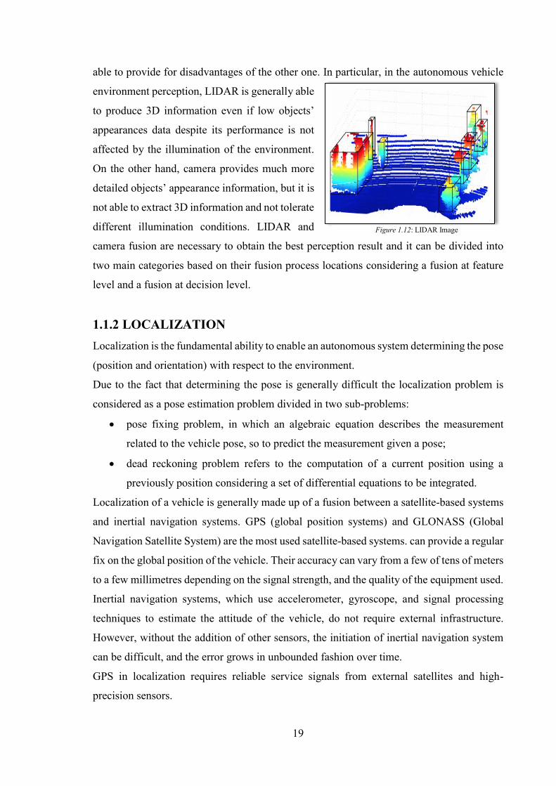
able to provide for disadvantages of the other one. In particular, in the autonomous vehicle

environment perception, LIDAR is generally able

to produce 3D information even if low objects’

appearances data despite its performance is not

affected by the illumination of the environment.

On the other hand, camera provides much more

detailed objects’ appearance information, but it is

not able to extract 3D information and not tolerate

different illumination conditions. LIDAR and

camera fusion are necessary to obtain the best perception result and it can be divided into

two main categories based on their fusion process locations considering a fusion at feature

level and a fusion at decision level.

1.1.2 LOCALIZATION Localization is the fundamental ability to enable an autonomous system determining the pose

(position and orientation) with respect to the environment.

Due to the fact that determining the pose is generally difficult the localization problem is

considered as a pose estimation problem divided in two sub-problems:

• pose fixing problem, in which an algebraic equation describes the measurement

related to the vehicle pose, so to predict the measurement given a pose;

• dead reckoning problem refers to the computation of a current position using a

previously position considering a set of differential equations to be integrated.

Localization of a vehicle is generally made up of a fusion between a satellite-based systems

and inertial navigation systems. GPS (global position systems) and GLONASS (Global

Navigation Satellite System) are the most used satellite-based systems. can provide a regular

fix on the global position of the vehicle. Their accuracy can vary from a few of tens of meters

to a few millimetres depending on the signal strength, and the quality of the equipment used.

Inertial navigation systems, which use accelerometer, gyroscope, and signal processing

techniques to estimate the attitude of the vehicle, do not require external infrastructure.

However, without the addition of other sensors, the initiation of inertial navigation system

can be difficult, and the error grows in unbounded fashion over time.

GPS in localization requires reliable service signals from external satellites and high-

precision sensors.

Figure 1.12: LIDAR Image

20

In recent years, map aided localization algorithms, like Simultaneous Localization and

Mapping (SLAM), have seen a remarkable advancement e trough local features it was

possible to achieve highly precise localization.

The SLAM goal is to create a map and use it simultaneously as it is built. SLAM algorithms

uses statistical modelling exploit old features observed by system sensors to estimate its

position in the map and identify new features even if the absolute position is almost

indefinable.

Bayesian filtering and smoothing are the main approaches used for solving the SLAM

problem formulated as an optimization problem to minimize the error.

1.1.3 PLANNING Planning refers to the process of making focused decisions in order to achieve the system’s

higher order goals, generally to move the vehicle from a starting location to a target location

avoiding obstacles and in the most optimal way as possible.

1.1.3.1 AUTONOMOUS VEHICLE PLANNING SYSTEMS The early stages of self-driving vehicles (SDV) were practically semi-autonomous in nature

and limited to functions and performance bases such as lane following or adaptive cruise

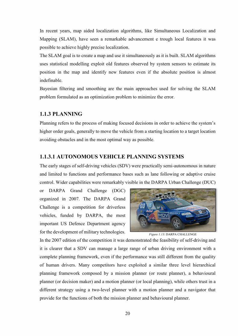
control. Wider capabilities were remarkably visible in the DARPA Urban Challenge (DUC)

or DARPA Grand Challenge (DGC)

organized in 2007. The DARPA Grand

Challenge is a competition for driverless

vehicles, funded by DARPA, the most

important US Defence Department agency

for the development of military technologies. In the 2007 edition of the competition it was demonstrated the feasibility of self-driving and

it is clearer that a SDV can manage a large range of urban driving environment with a

complete planning framework, even if the performance was still different from the quality

of human drivers. Many competitors have exploited a similar three level hierarchical

planning framework composed by a mission planner (or route planner), a behavioural

planner (or decision maker) and a motion planner (or local planning), while others trust in a

different strategy using a two-level planner with a motion planner and a navigator that

provide for the functions of both the mission planner and behavioural planner.

Figure 1.13: DARPA CHALLENGE

21

Each planner performs different objectives: the mission planner takes care of the high-level

task to achieve, such as which roads the vehicle should be taken; the behavioural planner has

to follow rules and restriction, makes in the proper way generating local task, such as change

lanes, overtake it, etc. Also, the motion planner has to achieve local objectives, typically

reach a target region without obstacle collision by generating suitable actions and proper

paths.

However, recent works continue to have this three-hierarchical planning framework.

1.1.3.2 MISSION PLANNING A graph network reflecting road and path network connectivity perform the mission

planning. In the DUC, the competition organizers manually generate a series of prior

information given as Route Network Definition File (RNDF) which represents road

segments through a graph of nodes and edges that includes information such as lane widths,

stop sign and parking locations. This type of information can be generated through

automated processes with sensing infrastructure or from direct deduction of vehicle motions.

Independently from the method, manual or automated, the path searching problem is linked

to a cost of traversing a road segment and subsequent graph search algorithms.

1.1.3.3 BEHAVIOURAL PLANNING The behavioural planner is important for making decisions on-board through Finite State

Machines (FSMs) of different complexity which ensure the interaction of vehicle with other

driving agents, the relative response and the respect of stipulated road rules during the

increase of the progress along the route prescribed by the mission planner.

This type of Finite State Machines is manually designed for a limited number of specific

situations and it can happen that the vehicle is in a situation not explicitly accounted for in

the FSM structure, for example in a livelock or in a deadlock state due to a lack of sufficient

deadlock protections.

Two terms involved in this phase planning are coined in order to categorize check functions

which control logical conditions occurred for certain state transition: (1) precedence

observers with the aim to check whether the rules related to the vehicle’s current location

allow to progress it; (2) clearance observers are needed in order to ensure and guarantee safe

clearance to the other traffic participants. In particular, they check the time collision which

the shortest time within which a detected obstacle enters in a certain interest region.

22

1.1.3.4 MOTION PLANNING Motion planning is a very large research field which space from an application to another

one: mobile robots, medicine, security and emergency situation, transportation and

agriculture. For example, motion planning applied in the mobile robots application refers to

the achievement of a specified goal after a decision process of an actions sequence, typically

avoiding collisions with obstacles.

For autonomous transportation, motion planning layer is those responsible for executing the

current motion target issued from the behaviours layer. In particular, the motion planner

creates a path for the desired goal, then tracks this path by generating a set of candidate

trajectories that follow the path and selecting from this set the best trajectory according to

an evaluation function. There are different types of evaluation function depending on the

context, but it’s a choice which includes consideration of static and dynamic obstacles, curbs,

speed, curvature, and deviation from the path. The selected trajectory can then be directly

executed by the vehicle.

Generally, different motion planners are evaluated and compared one each other in terms of

computational efficiency and completeness. Computational efficiency refers to the execution

time and to the scalability related to the configuration space dimension. Completeness is

related to an algorithm which in a finite time is considered complete. Moreover, this

algorithm always returns a solution when one exists and report in the contrary case.

Considering that motion planning problem has a huge computational complexity the

challenge became transforming the continuous space model into a discrete model. There are

two methods for approaching to this transformation:

• combinatorial planning, which perfectly represents the machines original problem

starting from a discrete representation;

• sampling-based planning, which apply a discrete sample searching from the

configuration space through a collision module.

1.1.3.5 COMBINATORIAL PLANNING Combinatorial planners have the function to find a complete solution starting from a built

discrete representation of the original problem. The combinatorial methods are limited in

application because the computational load increases with the configuration space dimension

and with the number of obstacles. For this reason, the sampling-based algorithms are more

used than the combinatorial ones.

23

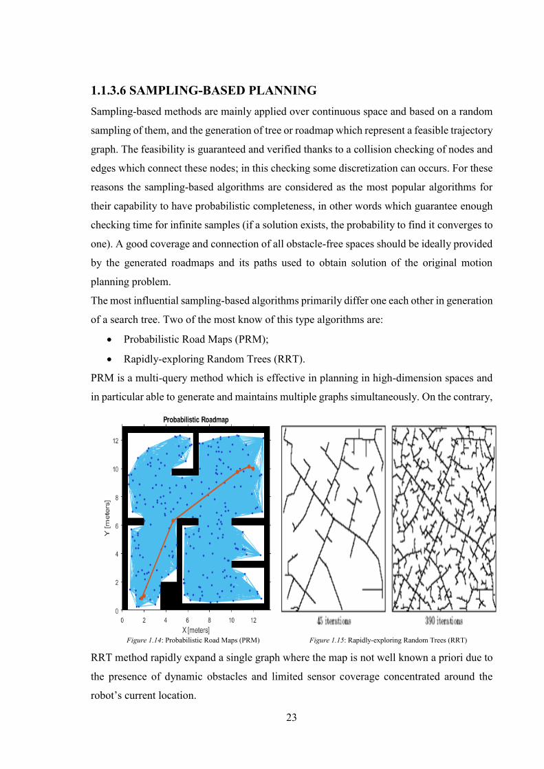
1.1.3.6 SAMPLING-BASED PLANNING Sampling-based methods are mainly applied over continuous space and based on a random

sampling of them, and the generation of tree or roadmap which represent a feasible trajectory

graph. The feasibility is guaranteed and verified thanks to a collision checking of nodes and

edges which connect these nodes; in this checking some discretization can occurs. For these

reasons the sampling-based algorithms are considered as the most popular algorithms for

their capability to have probabilistic completeness, in other words which guarantee enough

checking time for infinite samples (if a solution exists, the probability to find it converges to

one). A good coverage and connection of all obstacle-free spaces should be ideally provided

by the generated roadmaps and its paths used to obtain solution of the original motion

planning problem.

The most influential sampling-based algorithms primarily differ one each other in generation

of a search tree. Two of the most know of this type algorithms are:

• Probabilistic Road Maps (PRM);

• Rapidly-exploring Random Trees (RRT).

PRM is a multi-query method which is effective in planning in high-dimension spaces and

in particular able to generate and maintains multiple graphs simultaneously. On the contrary,

RRT method rapidly expand a single graph where the map is not well known a priori due to

the presence of dynamic obstacles and limited sensor coverage concentrated around the

robot’s current location.

Figure 1.14: Probabilistic Road Maps (PRM) Figure 1.15: Rapidly-exploring Random Trees (RRT)

24

The quality of the returned solutions is important in many applications, so it must be

considered together with completeness guarantees and efficiency in finding that solution. In

particular, in many cases it happens that a solution can be found quickly, but for a longer

period of time the algorithms continue to run in order to find better solutions based on some

heuristics. In the last years, starting from a research of lower cost solutions works, a complete

evaluation based on completeness, computational complexity, and optimality of many

popular planners was presented with a consecutive proposal of different sampling-based

planners and variants of PRM and RRT. From several studies it was highlighted that the

popular PRM and RRT algorithms are asymptotically sub-optimal, thus PRM* and RRT*

are proposed as asymptotically optimal variants of the first ones then other two variants such

as Fast Marching Trees (FMT*) and Stable Sparse Trees (SST*) are suggested to improve

the speed with respect to RRT*.

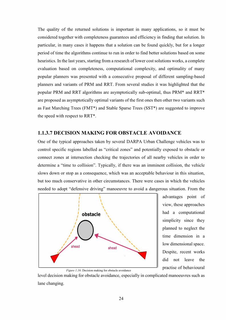
1.1.3.7 DECISION MAKING FOR OBSTACLE AVOIDANCE One of the typical approaches taken by several DARPA Urban Challenge vehicles was to

control specific regions labelled as “critical zones” and potentially exposed to obstacle or

connect zones at intersection checking the trajectories of all nearby vehicles in order to

determine a “time to collision”. Typically, if there was an imminent collision, the vehicle

slows down or stop as a consequence, which was an acceptable behaviour in this situation,

but too much conservative in other circumstances. There were cases in which the vehicles

needed to adopt “defensive driving” manoeuvre to avoid a dangerous situation. From the

advantages point of

view, these approaches

had a computational

simplicity since they

planned to neglect the

time dimension in a

low dimensional space.

Despite, recent works

did not leave the

practise of behavioural

level decision making for obstacle avoidance, especially in complicated manoeuvres such as

lane changing.

Figure 1.16: Decision making for obstacle avoidance

25

1.1.3.8 PLANNING IN SPACE-TIME It is necessary to include time as a dimension in the configuration space in order to consider

in a better way the obstacle movement, but this inclusion increases the problem complexity.

If, on the one hand, instantaneous position and velocity of obstacles may be detected, on the

other, it is yet difficult to predict future obstacle trajectories.

Previous approaches have used simple assumptions in predicting obstacle movement, such

as constant velocity trajectory with errors linked to a rapid iterative re-planning.

Starting from a situation in which it is possible to observe the instantaneous position and

velocity of obstacles, it follows that future obstacle trajectories can be predicted under the

common assumption of deterministic constant velocity which involves continuous

correction or verification through new observations.

Another possible method is to suppose a bounded velocity on obstacles which are

represented as conical volumes in space-time with a reduction of updating and re-planning.

Other type of on obstacles’ assumptions can be applied, such as static assumption and

assumption related to constant or bounded velocity and bounded acceleration, each of which

produce a limited volume of a different shape in space-time. A more cautious approach

would be to hypothesize a large area with the possible presence of obstacles, where the space

bounds of the obstacles grow over time based on the limitations of obstacle velocity or

acceleration firstly assumed. Obviously, an assumption to avoid would be the one in which

the uncertainty related to the prediction of an obstacle’s trajectory in the case of obstacle

bounded which does not grow over time is ignored. A possible solution can be the one in

which a direct plan in the control space is done avoiding specific type of control actions

which are predicted to lead to collision.

1.1.3.9 PLANNING SUBJECT TO DIFFERENTIAL CONSTRAINTS Motion planning is definitively a high-level control problem. Essentially, in order to obtain

simplicity or a computation reduction, the control limitations can be ignored in the different

levels of motion planner, but this can lead to dangerous operations related to inefficiencies

of trajectory and high control errors caused by the poor accounting on the constraints of the

system movement. One of the main problems which worries the collision control during the

planning phase is related to the discrepancies between the planned trajectory and the one that

is essentially performed, and this problem can represent a risk. The trajectories that can be

meticulously followed and with longer path length may tend to have shorter execution times

26

than those that are more difficult to follow, but with shorter path length. Paths can be directly

generated from sampling adequate controls, even if the paths won’t be optimized through

tree rewiring and popular asymptotically optimal planners, such as RRT* require sampling

from the configuration space. A possible challenging matter can be the incorporation of

differential constraints into state-sampling planners which requires a steering function able

to generate and draw an optimal path between two given states which are submitted to the

control constraints (if this path exists). Furthermore, querying methods are necessary to tell

whether a sampled state is reachable from a potential parent state.

The evolution of time is one of the most important differential constraints in a system, where

in general this time t increase at a constant rate t = 1 as imposition. Independently on the fact

that the time is explicitly included as a state parameter, other state parameters will generally

have differential constraints with respect to time, such as velocity and/or acceleration limits.

Differential constraints are applied to generate velocity profiles and can be solved in two

ways: along the geometric path chosen in a decoupled way, or simultaneously solving the

geometric path on each connection in the tree in a direct integrated way. The management

of the decoupled differential constraint can cause in very inefficient trajectories or not to find

a trajectory due to decoupling. On the other hand, the differential constraint managed in a

direct integrated manner can lead to improvements, but it’s computationally more complex.

Common limitations may be related to the radius of rotation that have often been resolved

through Dubins curves or Reeds-Shepp curves, which have been shown to ensure a shorter

distance given a minimum turning radius.

An efficient state sampling can be made more by limiting the sampled states to only those

from within a set of states known to be reachable from the initial condition given the system’s

kinodynamic constraints applied to an obstacle free environment. Similarly, it is only

convenient to check for connectivity between neighbouring states when they are part of each

other's reachable sets. Checking any states that are nearby according to Euclidean distance

metric but not reachable in a short period of time given kinodynamic constraints cause a

waste of computational effort. A possible solution can be adding Reachability Guidance

(RG) to state sampling and Nearest Neighbor (NN) searching which provide important

efficiency boosts to planning speed, especially for particular condition systems. These

systems can be those where motion is highly constrained or the motion checking cost is high.

In different recent works it was highlighted how the RG can be incorporated in the motion

planning through analytical approaches. To handle differential constraints, it is possible to

exploit an asymptotically optimal sampling-based algorithm, Goal-Rooted Feedback Motion

27

Tree (GR-FMT), restricted in application of controllable linear systems with linear

constraints. Furthermore, an important analytical method was presented in order to solving

a two-point boundary value problem subject to kinodynamic constraints. This method was

limited to systems with linear dynamics, but it could be used for finding optimal state-to-

state connections and NN searching.

Another important used approach was the machine learning approach which had the aim to

verify whether a state was reachable from a given base state, even though this method

required the application of a Support Vector Machine SVM classifier over a 36-feature set

for the Dubins car model which could be extremely expensive from the computation point

of view.During the recent years there were also relatively few planning effective methods

for solving over a configuration space having an appended time. Every job has taken a

different path: some explored control sampling approaches providing model simplifications

to handle the differential constraints in an online manner, others have performed planning

with discrete, time-bounded lattice structure based on motion primitives, or a grid cell

decomposition of the state space.

1.1.3.10 INCREMENTAL PLANNING AND REPLANNING The most common challenges in the autonomous vehicle planning are mainly related to the

limited perception range and the dynamic nature of operating environments. Typically, the

sensing range is limited not only by sensor specifications, but also reduced for the presences

of obstacles which obstructs the view.

It often happens that the system will not be able to perceive the entire path from a starting

location to goal location at any one specific instant of time. Thus, for this reason there is the

need to generate incremental plans in order to follow trajectories which allow to forward

progress towards the final goal location.

One key aspect to consider is that the system performs its planned trajectory, but other

mobile agents who have their own objectives can move unexpectedly. Therefore, the

environment changes continuously and those trajectories that in a prior time instant are

considered safe, in a subsequent time instant may no longer be so. For this reason, it is

necessary to apply a substitution in order to regulate the dynamic changes of the

environment. This incremental planning mechanism requires a means to generate

incremental sub-targets, or alternatively to choose the best trajectory between a set of

possible trajectories based on some heuristics.

28

At least a new plan must be generated with the same frequency of new sub-goal definitions.

Given the different planning situation can happens in some cases that no sub-goals were

defined or there wasn't a predefined path and thus, the best choice are the trajectories selected

based on a combined weighted heuristic of trajectory execution time and distance to goal

from the end trajectory state. Bouraine et al. have applied a constant rate replanning timer in

which each current solution plan was executed concurrently with the generation of

subsequent plan, and each newly planned trajectory would be rooted from an anticipated

committed pose given the previous committed solution trajectory.

Replanning in iterative way to generate new solution trajectories represents a potential

opportunity to transfer knowledge from previous planning iterations to subsequent ones. If

prior planning information is well utilized while a new plan could start from scratch, better

solutions may be found faster. In other works, it is suggested that redoing collision-checks

over the entire planning tree, as in Dynamic RRT (DRRT), in which the tree structure was

utilized to trim child “branches” once a parent state was found to be no longer valid.

Recently, it was presented a replanning variant of RRT*, RRTX, which trims the previous

planning iteration’s planning tree, but efficiently reconnects disconnected branches to other

parts of the tree maintaining the rewiring principal of RRT* responsible for asymptotic

optimality.

Safety mechanisms are an aspect that should also be carefully designed considering that a

finite time for computation are required for each planning cycle and the environment may

change during that time. The problem of obstacle presence has as response passive safety

mechanisms prescribed by several works, where passive safety refers to the ability to avoid

collision while the system is moving. In general, velocity planning was decoupled from the

path planning, and a particular approach called “Dynamic Virtual Bumper” would prescribe

reduced speed based on the proximity of the nearest obstacle as measured by a weighted

longitudinal and lateral offset from the desired path. In particular, moving obstacles were

treated as enlarged static obstacles with the assumption that they occupied the area traced by

their current constant velocity trajectory over a short time frame in addition to their current

spatial location. [5]

29

CHAPTER 2

AUTONOMOUS PARKING

30

AUTONOMOUS PARKING 2. AUTONOMOUS PARKING EVOLUTION The first approach to autonomous parking was in the early 2000s when a parking assistance

technology was implemented by using sensors or cameras helping the driver to control the

parking manoeuvre.

The main parking sensor used was the ultrasonic sensor that can detect objects through the

use if high frequency sound waves. The sensor is installed on the rear part of vehicle;

therefore, it can help the driver to detect a wall or another vehicle during parking. A receiver

detects these waves and calculates the distance from the object to vehicle, in the case when

the object is too close to the vehicle, the driver is warned via a continuous beep noise which

becomes more rapid the closer the car is from the object.

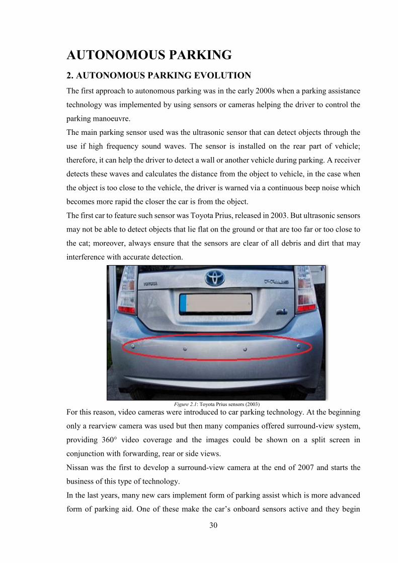
The first car to feature such sensor was Toyota Prius, released in 2003. But ultrasonic sensors

may not be able to detect objects that lie flat on the ground or that are too far or too close to

the cat; moreover, always ensure that the sensors are clear of all debris and dirt that may

interference with accurate detection.

For this reason, video cameras were introduced to car parking technology. At the beginning

only a rearview camera was used but then many companies offered surround-view system,

providing 360° video coverage and the images could be shown on a split screen in

conjunction with forwarding, rear or side views.

Nissan was the first to develop a surround-view camera at the end of 2007 and starts the

business of this type of technology.

In the last years, many new cars implement form of parking assist which is more advanced

form of parking aid. One of these make the car’s onboard sensors active and they begin

Figure 2.1: Toyota Prius sensors (2003)

31

scanning for appropriate parking spaces determining whether space is of a reasonable size

for parking the car. Another functionality shows the intended reverse course via onboard

multifunctional display, the driver need not to take control of steering wheel which allows

him to retain full control of the clutch, accelerator and brake.

First version of park assist was introduced in 2003 but it has become widely available in the

last years, especially Kia and Ford.

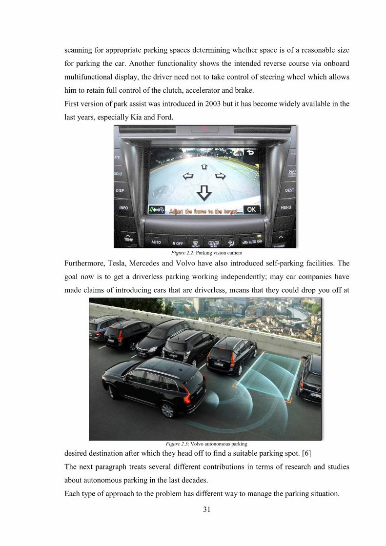
Furthermore, Tesla, Mercedes and Volvo have also introduced self-parking facilities. The

goal now is to get a driverless parking working independently; may car companies have

made claims of introducing cars that are driverless, means that they could drop you off at

desired destination after which they head off to find a suitable parking spot. [6]

The next paragraph treats several different contributions in terms of research and studies

about autonomous parking in the last decades.

Each type of approach to the problem has different way to manage the parking situation.

Figure 2.2: Parking vision camera

Figure 2.3: Volvo autonomous parking

32

2.1 DIRECT TRAJECTORY PLANNING: HUMAN-LIKE PARKING The problem related to the parking control remain something to be solved for autonomous

vehicles. Generally, the approaches that already exist first design a parking reference

trajectory that does not exactly respect vehicle dynamic constraints and second apply

specific online negative feedback control to make the vehicle roughly track this reference

trajectory.

The main purpose of designing autonomous vehicles is to complete most driving tasks

instead of human drivers. These tasks requirements become complicated also for low speed

scenario met by every driver in each day: traffic and parking scenario.

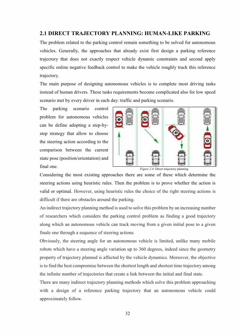
The parking scenario control

problem for autonomous vehicles

can be define adopting a step-by-

step strategy that allow to choose

the steering action according to the

comparison between the current

state pose (position/orientation) and

final one.

Considering the most existing approaches there are some of these which determine the

steering actions using heuristic rules. Then the problem is to prove whether the action is

valid or optimal. However, using heuristic rules the choice of the right steering actions is

difficult if there are obstacles around the parking.

An indirect trajectory planning method is used to solve this problem by an increasing number

of researchers which considers the parking control problem as finding a good trajectory

along which an autonomous vehicle can track moving from a given initial pose to a given

finale one through a sequence of steering actions.

Obviously, the steering angle for an autonomous vehicle is limited, unlike many mobile

robots which have a steering angle variation up to 360 degrees, indeed since the geometry

property of trajectory planned is affected by the vehicle dynamics. Moreover, the objective

is to find the best compromise between the shortest length and shortest time trajectory among

the infinite number of trajectories that create a link between the initial and final state.

There are many indirect trajectory planning methods which solve this problem approaching

with a design of a reference parking trajectory that an autonomous vehicle could

approximately follow.

Figure 2.4: Direct trajectory planning

33

Typically, the reference trajectories are particular curves like β-spline curves or polynomial

curves with specific geometric properties to obtain a simplification of planning and

presentation of the desired trajectories. The gap between the real actual trajectory through

the application of the correspondent steering actions and reference parking trajectory will be

restricted by means a negative feedback controller to reshape the steering actions and make

the vehicle approximately track this reference trajectory. However, it is important to consider

that the gap can vary, and it could have deviations along the different part of the trajectory

which could cause collision with the obstacles around especially in reverse parking

situations.

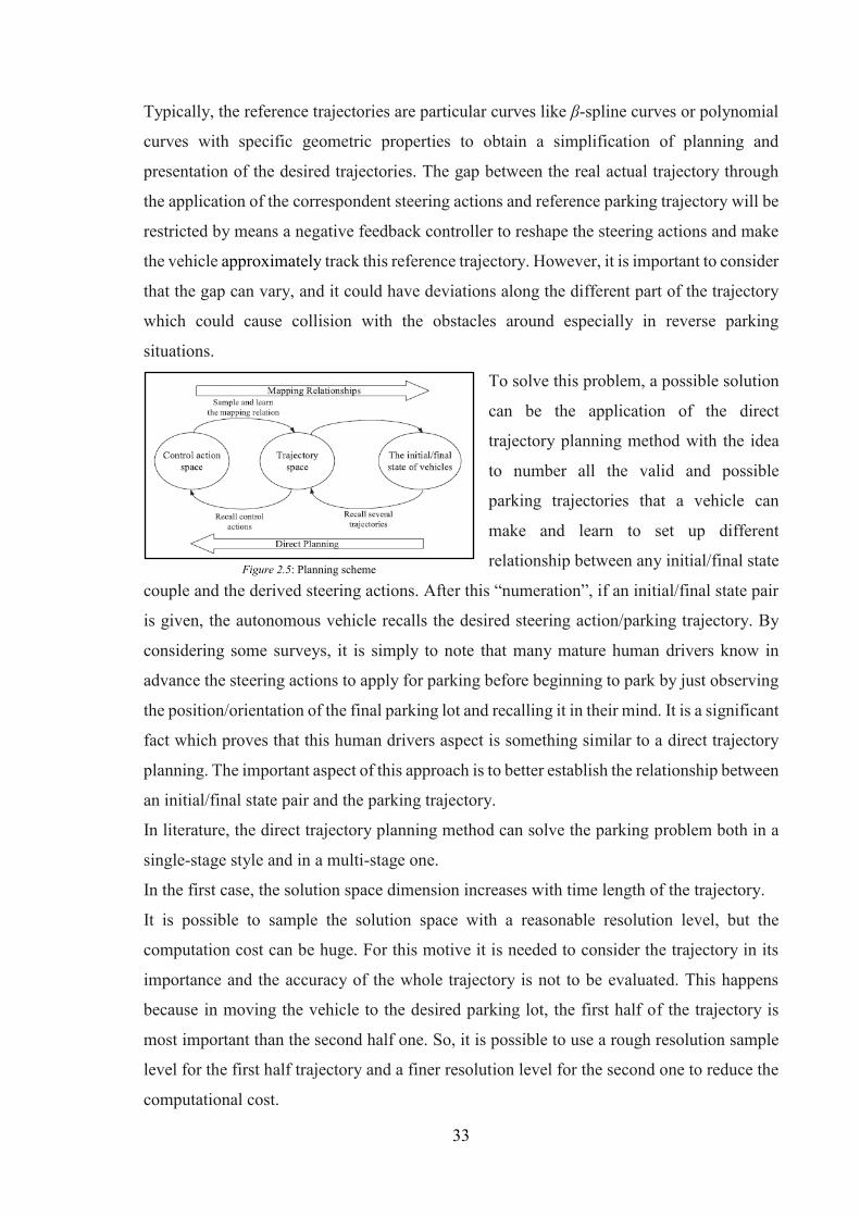
To solve this problem, a possible solution

can be the application of the direct

trajectory planning method with the idea

to number all the valid and possible

parking trajectories that a vehicle can

make and learn to set up different

relationship between any initial/final state

couple and the derived steering actions. After this “numeration”, if an initial/final state pair

is given, the autonomous vehicle recalls the desired steering action/parking trajectory. By

considering some surveys, it is simply to note that many mature human drivers know in

advance the steering actions to apply for parking before beginning to park by just observing

the position/orientation of the final parking lot and recalling it in their mind. It is a significant

fact which proves that this human drivers aspect is something similar to a direct trajectory

planning. The important aspect of this approach is to better establish the relationship between

an initial/final state pair and the parking trajectory.

In literature, the direct trajectory planning method can solve the parking problem both in a

single-stage style and in a multi-stage one.

In the first case, the solution space dimension increases with time length of the trajectory.

It is possible to sample the solution space with a reasonable resolution level, but the

computation cost can be huge. For this motive it is needed to consider the trajectory in its

importance and the accuracy of the whole trajectory is not to be evaluated. This happens

because in moving the vehicle to the desired parking lot, the first half of the trajectory is

most important than the second half one. So, it is possible to use a rough resolution sample

level for the first half trajectory and a finer resolution level for the second one to reduce the

computational cost.

Figure 2.5: Planning scheme

34

Another well-known feature, based on a series of considerations, to describe the vehicle

movements with the direct planning method is that to a dynamic model rather than a

kinematic model. First, the general trajectory planning method is designed not only for the

parking problem, but it is also extended for other vehicle motion planning/control problems.

Second, the complexity of the conventional indirect trajectory planning method that use

kinematic model for vehicle movements is greater than direct trajectory planning methods.

In a direct planning approach, the design cost of a controller is saved, while in a kinematic

approach it is needed to design a controller make and cost increases the calculation

complexity. Third, it is very difficult to obtain a very strict gap between the ideal trajectories

and the obtained one in indirect trajectory planning methods. Fourth, using the direct

planning method, it is possible to not consider vehicle kinematic models with very low speed

requirements.

Furthermore, it is possible to assimilate in the same manner both the front steering vehicles

parking problem and the full steering vehicles one.

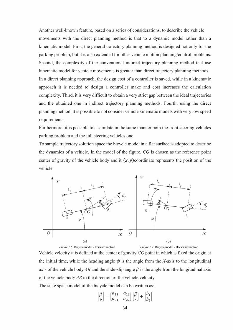
To sample trajectory solution space the bicycle model in a flat surface is adopted to describe

the dynamics of a vehicle. In the model of the figure, CG is chosen as the reference point

center of gravity of the vehicle body and it (𝑥, 𝑦)coordinate represents the position of the

vehicle.

Vehicle velocity 𝑣 is defined at the center of gravity CG point in which is fixed the origin at

the initial time, while the heading angle 𝜓 is the angle from the X-axis to the longitudinal

axis of the vehicle body AB and the slide-slip angle 𝛽 is the angle from the longitudinal axis

of the vehicle body AB to the direction of the vehicle velocity.

The state space model of the bicycle model can be written as:

[����] = [

𝑎11 𝑎12𝑎21 𝑎22

] [𝛽𝑟] + [

𝑏1𝑏2]

Figure 2.6: Bicycle model - Forward motion Figure 2.7: Bicycle model - Backward motion

35

with coefficients

𝑎11 = −𝑐𝑓 + 𝑐𝑟

𝑚𝑣𝑎12 = −1 −

𝑐𝑓𝑙𝑓 + 𝑐𝑟𝑙𝑟

𝑚𝑣2

𝑎21 = −𝑐𝑓𝑙𝑓 + 𝑐𝑟𝑙𝑟

𝐼𝑎22 = −

𝑐𝑓𝑙𝑓2 + 𝑐𝑟𝑙𝑟

2

𝐼𝑣

𝑏1 =𝑐𝑓

𝑚𝑣𝑏2 =

𝑐𝑓𝑙𝑓

𝐼

The direction of the positive X-axis is assumed to point to the head of the vehicle, while 𝑣𝑥

and 𝑣𝑦 are the projection of the velocity 𝑣 onto the 𝑋, 𝑌 axes.

If the vehicle goes forward the equations are the follows:

𝑣𝑥 = 𝑣𝑐𝑜𝑠(𝛽 + 𝜓)

𝑣𝑦 = 𝑣𝑠𝑖𝑛(𝛽 + 𝜓)

while, if the vehicle goes backward the equations became the follows:

𝑣𝑥 = −𝑣𝑐𝑜𝑠(𝛽 + 𝜓)

𝑣𝑦 = 𝑣𝑠𝑖𝑛(𝛽 + 𝜓)

Thanks to these equations it is possible to calculate the position and the orientation of the

vehicle during the parking.

Symbol Meaning Value

𝑋 − 𝑌 Coordinate system

𝛽 Vehicle sideslip angle

𝜓 Heading angle

𝑟 Yaw rate of the vehicle, 𝑟 = 𝜓

𝛿𝑓 Front steering angle

𝑣 Vehicle velocity

𝛿𝑚𝑎𝑥 Maximum of the front steering angle 0.6 rad

𝑚 Mass of the vehicle 1500 kg

𝐼 Inertia moment around the vertical axis

through CG 2500 𝑘𝑔 ∙ 𝑚2

𝑙𝑓 Distance from point A and point CG 1.20 m

𝑙𝑟 Distance from point B and point CG 1.50 m

𝑐𝑓 Front tire stiffness coefficients 80000 N/rad

𝑐𝑟 Rear tire stiffness coefficients 80000 N/rad

36

Given the value of input vehicle speed and front steering angle within a time range the

resulting trajectory of the vehicle is calculable based on the dynamic model that allow to

generate a sample mapping relation between the two variables and the trajectory. To obtain

a complex and richer mapping relation it can be assumed that the vehicle keeps a low velocity

of 1/ms during the whole parking process, from the starting process to the stopping one

(instantaneous parking assumption). If enough samples are obtained, a mapping relation is

more simply to organize.

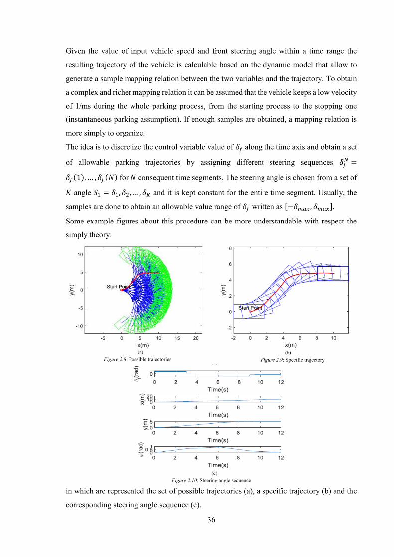
The idea is to discretize the control variable value of 𝛿𝑓 along the time axis and obtain a set

of allowable parking trajectories by assigning different steering sequences 𝛿𝑓𝑁 =

𝛿𝑓(1),… , 𝛿𝑓(𝑁) for 𝑁 consequent time segments. The steering angle is chosen from a set of

𝐾 angle 𝑆1 = 𝛿1, 𝛿2, … , 𝛿𝐾 and it is kept constant for the entire time segment. Usually, the

samples are done to obtain an allowable value range of 𝛿𝑓 written as [−𝛿𝑚𝑎𝑥, 𝛿𝑚𝑎𝑥].

Some example figures about this procedure can be more understandable with respect the

simply theory:

in which are represented the set of possible trajectories (a), a specific trajectory (b) and the

corresponding steering angle sequence (c).

Figure 21: Possible trajectories Figure 2.8: Possible trajectories Figure 2.9: Specific trajectory

Figure 2.10: Steering angle sequence

37

The Single-Stage direct trajectory planning is based on the whole control action sequence

generated at the beginning of the parking process and the difference with respect to the

indirect trajectory planning method is that in this last case the trajectory is generated by

vehicle dynamics, while in the first case through approximated curves.

All the found trajectories of the SSDP are stored in discrete form as a consecutive series of

states thanks to a discretization with a specific chosen time interval. R1 will denote the final

obtained trajectory and a threshold is set in order to understand if a given final state can be

matched with a stored trajectory by controlling the distance between this state and R1.

Since there exist lots of trajectories, the important trajectory to be stored is the optimal one

and to do this a performance index of a trajectory is defined:

𝐽 = ∫ (𝑣(𝑡) + 𝛿𝑓2(𝑡) + 𝑐(𝑡)) 𝑑𝑡 +

𝜏

0

[ℎ(𝑥𝜏,𝑦𝜏, 𝜓𝜏) − ℎ(𝑥𝑝𝑦𝑝, 𝜓𝑝)]2

with 𝜏 terminal time, 𝑐(𝑡) curvature at time 𝑡 along the trajectory, (𝑥𝜏,𝑦𝜏, 𝜓𝜏) final state of

the vehicle and (𝑥𝑝𝑦𝑝, 𝜓𝑝) stop state of the vehicle at the parking lot center.

ℎ is the surface integral of the function 𝑓(𝑥, 𝑦) with respect to the rectangular region 𝐷𝑡

which represents the vehicle at the state (𝑥𝜏,𝑦𝜏, 𝜓𝜏) .

ℎ(𝑥𝜏,𝑦𝜏, 𝜓𝜏) = ∬𝑓(𝑥, 𝑦)𝑑𝜎

𝐷𝑡

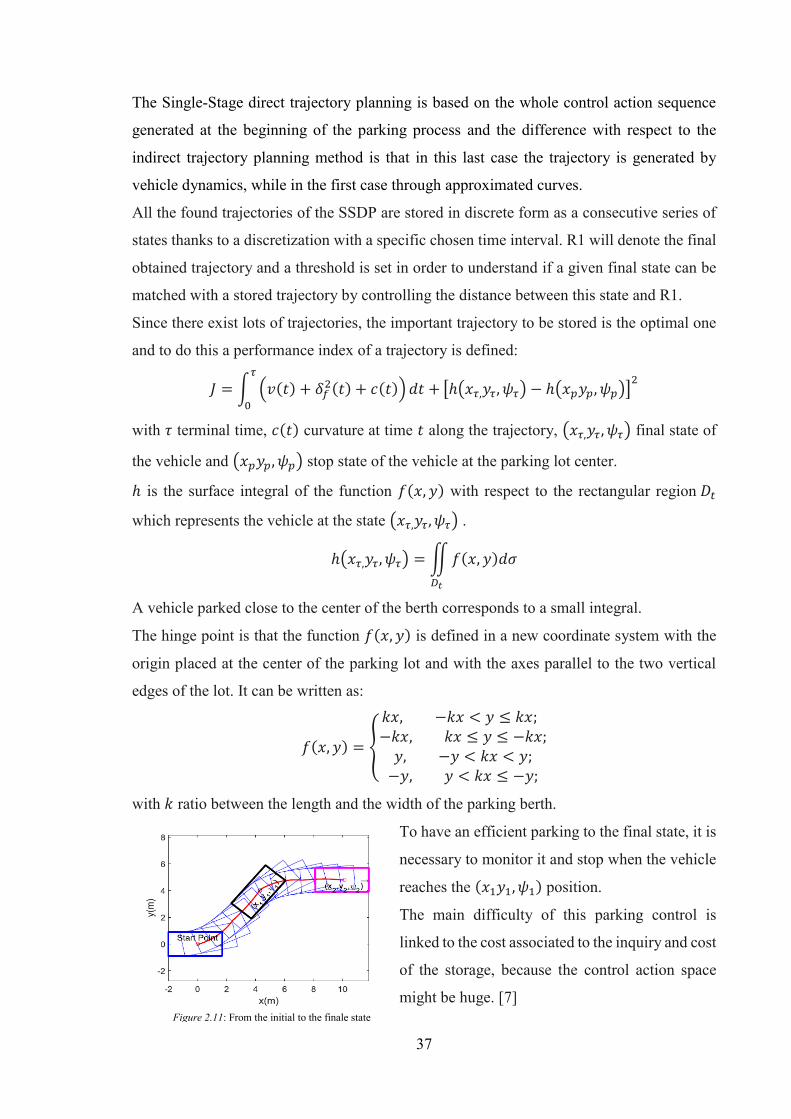
A vehicle parked close to the center of the berth corresponds to a small integral.

The hinge point is that the function 𝑓(𝑥, 𝑦) is defined in a new coordinate system with the

origin placed at the center of the parking lot and with the axes parallel to the two vertical

edges of the lot. It can be written as:

𝑓(𝑥, 𝑦) = {

𝑘𝑥, −𝑘𝑥 < 𝑦 ≤ 𝑘𝑥; −𝑘𝑥, 𝑘𝑥 ≤ 𝑦 ≤ −𝑘𝑥;𝑦, −𝑦 < 𝑘𝑥 < 𝑦;−𝑦, 𝑦 < 𝑘𝑥 ≤ −𝑦;

with 𝑘 ratio between the length and the width of the parking berth.

To have an efficient parking to the final state, it is

necessary to monitor it and stop when the vehicle

reaches the (𝑥1𝑦1, 𝜓1) position.

The main difficulty of this parking control is

linked to the cost associated to the inquiry and cost

of the storage, because the control action space

might be huge. [7] Figure 2.11: From the initial to the finale state

38

2.2 INTELLEGENT AUTONOMOUS PARKING CONTROL SYSTEM A parking trajectory can be planned starting from a mathematical formulation of the problem

based on finding the minimum length of the trajectory and minimum number of maneuver

space. Parking control of this type can be based on the fuzzy logic evaluating the problem

from three aspects:

• detection of the parking berth;

• evaluation of the present position and path generation;

• trajectory correction through the motion.

For the first aspect, the spatial orientation and parking detection control are managed by

means a lot of sensors such as lidars, laser scanners, video sensors, ultrasonic sensors or

cameras.

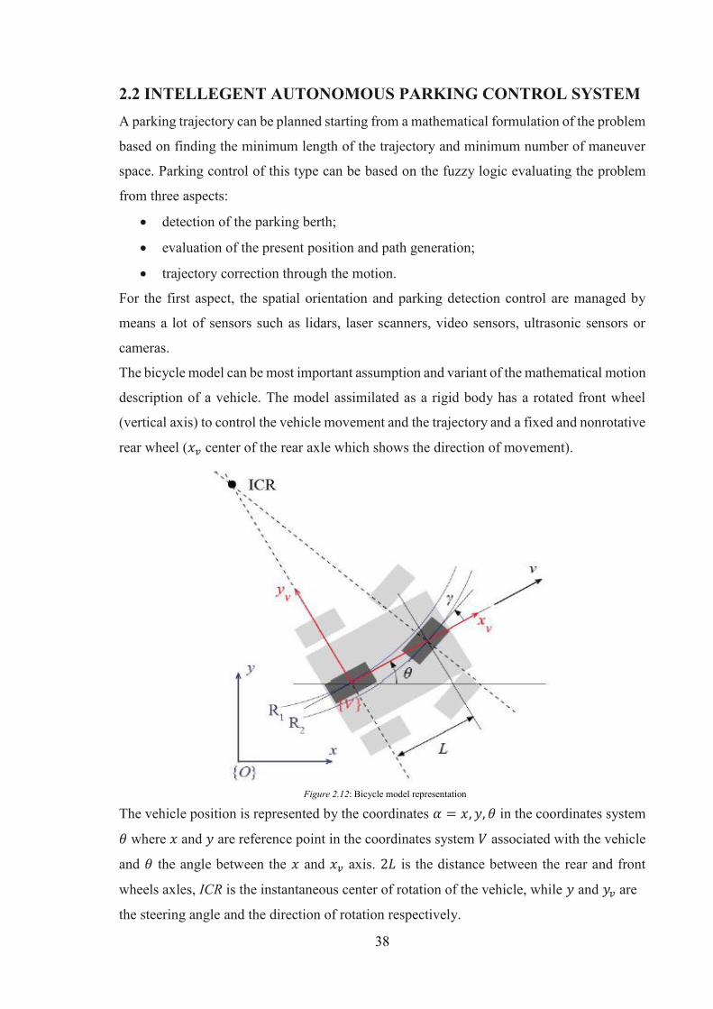
The bicycle model can be most important assumption and variant of the mathematical motion

description of a vehicle. The model assimilated as a rigid body has a rotated front wheel

(vertical axis) to control the vehicle movement and the trajectory and a fixed and nonrotative

rear wheel (𝑥𝑣 center of the rear axle which shows the direction of movement).

The vehicle position is represented by the coordinates 𝛼 = 𝑥, 𝑦, 𝜃 in the coordinates system

𝜃 where 𝑥 and 𝑦 are reference point in the coordinates system 𝑉 associated with the vehicle

and 𝜃 the angle between the 𝑥 and 𝑥𝑣 axis. 2𝐿 is the distance between the rear and front

wheels axles, ICR is the instantaneous center of rotation of the vehicle, while 𝑦 and 𝑦𝑣 are

the steering angle and the direction of rotation respectively.

Figure 2.12: Bicycle model representation

39

The relation and dependence between orientation, rotation angle of the steering wheels,

vehicle velocity and vehicle current position coordinates are described by this equation

system:

{

�� = 𝑣 ∙ sin 𝜃

�� =𝑣

𝐿∙ tan 𝛾

�� = 𝑣 ∙ cos 𝜃

through the geometric transformations it is possible to determine the velocity projection of

the plant in 𝑂 coordinates systems on 𝑦 axis in the coordinates system 𝑉.

�� 𝑐𝑜𝑠 𝜃 − �� 𝑠𝑖𝑛 𝜃 = 0

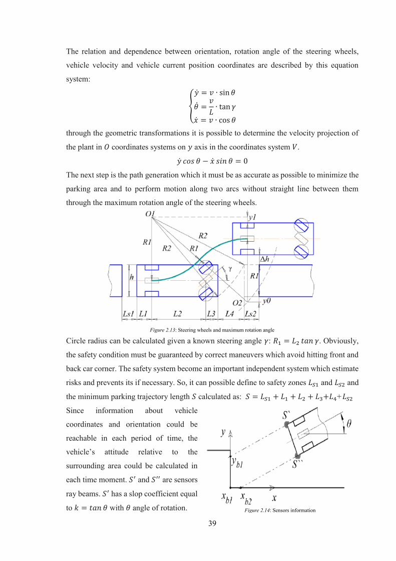
The next step is the path generation which it must be as accurate as possible to minimize the

parking area and to perform motion along two arcs without straight line between them

through the maximum rotation angle of the steering wheels.

Circle radius can be calculated given a known steering angle 𝛾: 𝑅1 = 𝐿2 𝑡𝑎𝑛 𝛾. Obviously,

the safety condition must be guaranteed by correct maneuvers which avoid hitting front and

back car corner. The safety system become an important independent system which estimate

risks and prevents its if necessary. So, it can possible define to safety zones 𝐿𝑆1 and 𝐿𝑆2 and

the minimum parking trajectory length 𝑆 calculated as: 𝑆 = 𝐿𝑆1 + 𝐿1 + 𝐿2 + 𝐿3+𝐿4+𝐿𝑆2

Since information about vehicle

coordinates and orientation could be

reachable in each period of time, the

vehicle’s attitude relative to the

surrounding area could be calculated in

each time moment. 𝑆′ and 𝑆′′ are sensors

ray beams. 𝑆′ has a slop coefficient equal

to 𝑘 = 𝑡𝑎𝑛 𝜃 with 𝜃 angle of rotation. Figure 2.14: Sensors information

Figure 2.13: Steering wheels and maximum rotation angle

40

The piercing point of a line corresponding to the sensor’s ray beam with axes of refence

coordinate system could be calculated with this equation:

𝑦𝑏1 = 𝑘 ∙ 𝑥𝑏1 + 𝑏

which allow to obtain the coordinate of the piercing point 𝑥𝑏1 and 𝑦𝑏1 that are the limit points

of safety maneuver completion zone.

The sensors coordinate must be converted into reference coordinate system in order to find

coefficient 𝑏:

𝑏 = 𝑦𝑝0 − 𝑡𝑎𝑛 𝜃 ∙ 𝑥𝑝

0

where 𝑥𝑝0 and 𝑦𝑝0 are the distance coordinates of the sensor in reference coordinate system.

For the sensor 𝑆′ the body axes coordinates are stored in the vector 𝑣𝑝:

𝑣𝑝 = [

𝑥𝑠1𝑦𝑠1

0]

that then converted in reference coordinate system become the following ones:

𝑣𝑝0 = [

𝑐𝑜𝑠 𝜃 𝑠𝑖𝑛 𝜃 0−𝑠𝑖𝑛 𝜃0

𝑐𝑜𝑠 𝜃0

01] [

𝑥𝑠1𝑦𝑠1

0] + [

𝑥𝑣0

𝑦𝑣0

0

] = [

𝑥𝑝0

𝑦𝑝0

0

]

The minimal safety distance to the nearest obstacle could be calculated in this way:

𝑙𝑚𝑎𝑥1 = √𝑙𝑥2 + 𝑙𝑦2 = √(𝑥𝑝0 − 𝑥𝑏1)2 + (𝑦𝑝

0 − 𝑦𝑏1)2

this algorithm allows to realize the fuzzy controller which performance are base on

information about normalized distance to obstacle calculated as follows:

𝑙𝑛1 =𝑙𝑠1𝑙𝑚𝑎𝑥1

where 𝑙𝑠1 is the distance derived from the sensor 𝑆′.

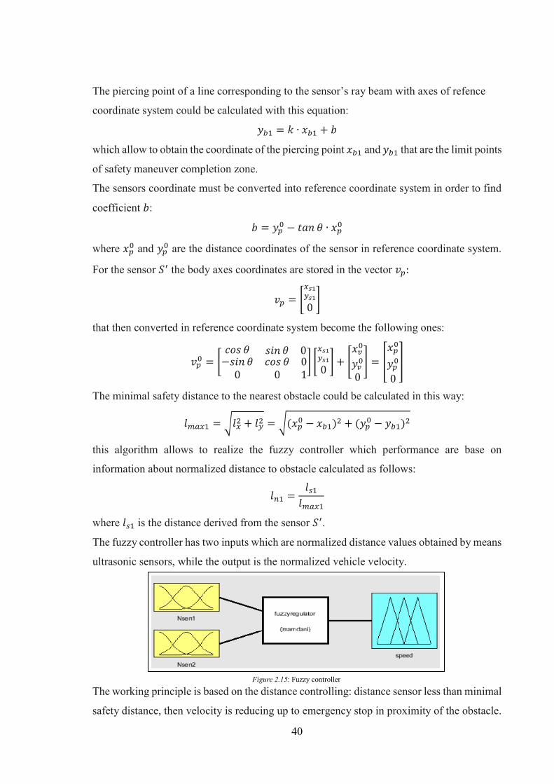
The fuzzy controller has two inputs which are normalized distance values obtained by means

ultrasonic sensors, while the output is the normalized vehicle velocity.

The working principle is based on the distance controlling: distance sensor less than minimal

safety distance, then velocity is reducing up to emergency stop in proximity of the obstacle.

Figure 2.15: Fuzzy controller

41

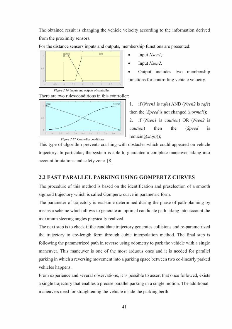
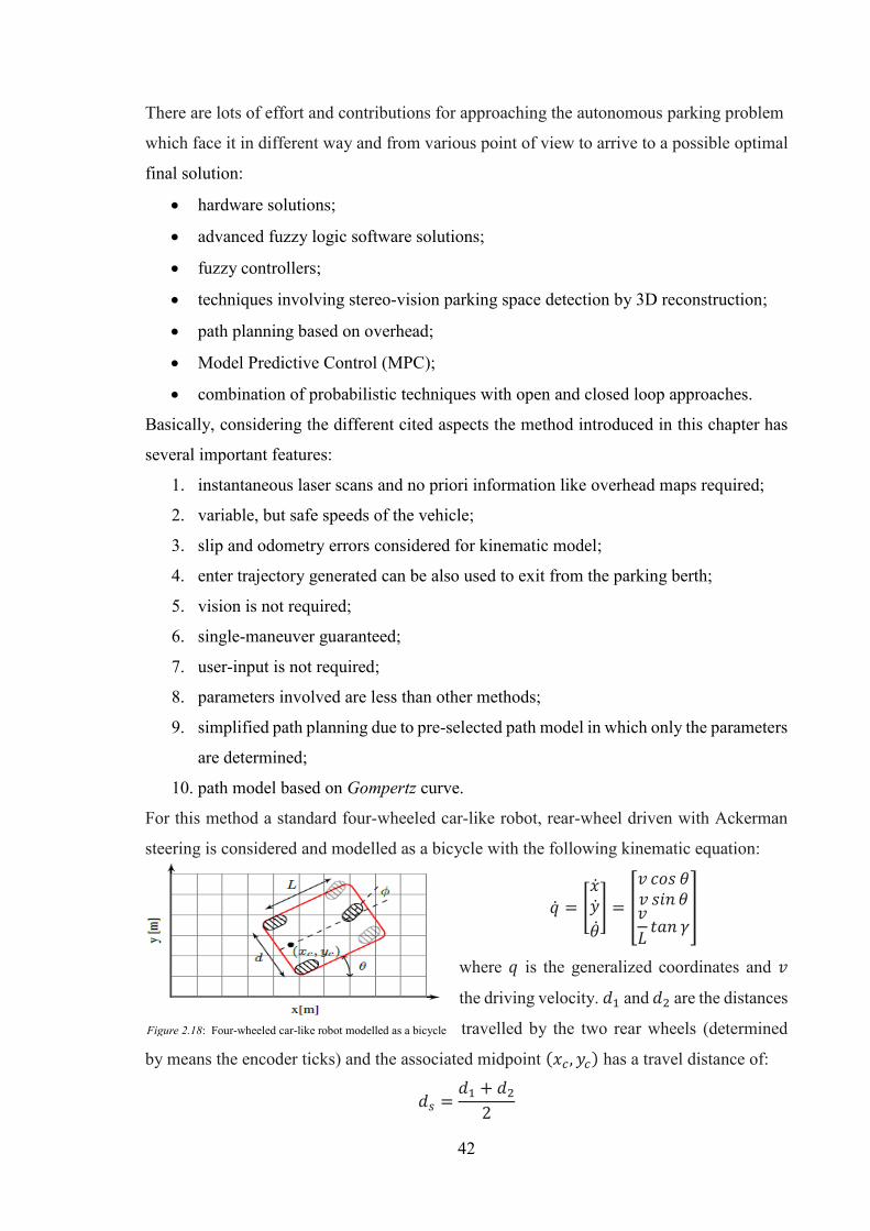
The obtained result is changing the vehicle velocity according to the information derived

from the proximity sensors.

For the distance sensors inputs and outputs, membership functions are presented:

• Input Nsen1;

• Input Nsen2;

• Output includes two membership

functions for controlling vehicle velocity.

There are two rules/conditions in this controller:

1. if (Nsen1 is safe) AND (Nsen2 is safe)

then the (Speed is not changed (normal));

2. if (Nsen1 is caution) OR (Nsen2 is

caution) then the (Speed is

reducing(stop)));

This type of algorithm prevents crashing with obstacles which could appeared on vehicle

trajectory. In particular, the system is able to guarantee a complete maneuver taking into

account limitations and safety zone. [8]

2.2 FAST PARALLEL PARKING USING GOMPERTZ CURVES The procedure of this method is based on the identification and preselection of a smooth

sigmoid trajectory which is called Gompertz curve in parametric form.

The parameter of trajectory is real-time determined during the phase of path-planning by

means a scheme which allows to generate an optimal candidate path taking into account the

maximum steering angles physically realized.

The next step is to check if the candidate trajectory generates collisions and re-parametrized

the trajectory to arc-length form through cubic interpolation method. The final step is

following the parametrized path in reverse using odometry to park the vehicle with a single

maneuver. This maneuver is one of the most arduous ones and it is needed for parallel

parking in which a reversing movement into a parking space between two co-linearly parked

vehicles happens.

From experience and several observations, it is possible to assert that once followed, exists

a single trajectory that enables a precise parallel parking in a single motion. The additional

maneuvers need for straightening the vehicle inside the parking berth.

Figure 2.16: Inputs and outputs of controller

Figure 2.17: Controller conditions

42

There are lots of effort and contributions for approaching the autonomous parking problem

which face it in different way and from various point of view to arrive to a possible optimal

final solution:

• hardware solutions;

• advanced fuzzy logic software solutions;

• fuzzy controllers;

• techniques involving stereo-vision parking space detection by 3D reconstruction;

• path planning based on overhead;

• Model Predictive Control (MPC);

• combination of probabilistic techniques with open and closed loop approaches.

Basically, considering the different cited aspects the method introduced in this chapter has

several important features:

1. instantaneous laser scans and no priori information like overhead maps required;

2. variable, but safe speeds of the vehicle;

3. slip and odometry errors considered for kinematic model;

4. enter trajectory generated can be also used to exit from the parking berth;

5. vision is not required;

6. single-maneuver guaranteed;

7. user-input is not required;

8. parameters involved are less than other methods;

9. simplified path planning due to pre-selected path model in which only the parameters

are determined;

10. path model based on Gompertz curve.

For this method a standard four-wheeled car-like robot, rear-wheel driven with Ackerman

steering is considered and modelled as a bicycle with the following kinematic equation:

�� = [����

��

] = [

𝑣 𝑐𝑜𝑠 𝜃𝑣 𝑠𝑖𝑛 𝜃𝑣

𝐿𝑡𝑎𝑛 𝛾

]

where 𝑞 is the generalized coordinates and 𝑣

the driving velocity. 𝑑1 and 𝑑2 are the distances

travelled by the two rear wheels (determined

by means the encoder ticks) and the associated midpoint (𝑥𝑐, 𝑦𝑐) has a travel distance of:

𝑑𝑠 =𝑑1 + 𝑑22

Figure 2.18: Four-wheeled car-like robot modelled as a bicycle

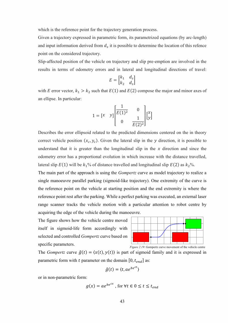
43

which is the reference point for the trajectory generation process.

Given a trajectory expressed in parametric form, its parametrized equations (by arc-length)

and input information derived from 𝑑𝑠 it is possible to determine the location of this refence

point on the considered trajectory.

Slip-affected position of the vehicle on trajectory and slip pre-emption are involved in the

results in terms of odometry errors and in lateral and longitudinal directions of travel:

𝐸 = [𝑘1 𝑑𝑠𝑘2 𝑑𝑠

]

with 𝐸 error vector, 𝑘1 > 𝑘2 such that 𝐸(1) and 𝐸(2) compose the major and minor axes of

an ellipse. In particular:

1 = [𝑥 𝑦]

[ 1

𝐸(1)20

01

𝐸(2)2]

[𝑥𝑦]

Describes the error ellipsoid related to the predicted dimensions centered on the in theory

correct vehicle position (𝑥𝑐, 𝑦𝑐). Given the lateral slip in the 𝑦 direction, it is possible to

understand that it is greater than the longitudinal slip in the 𝑥 direction and since the

odometry error has a proportional evolution in which increase with the distance travelled,

lateral slip 𝐸(1) will be 𝑘1% of distance travelled and longitudinal slip 𝐸(2) as 𝑘2%.

The main part of the approach is using the Gompertz curve as model trajectory to realize a

single manoeuvre parallel parking (sigmoid-like trajectory). One extremity of the curve is

the reference point on the vehicle at starting position and the end extremity is where the

reference point rest after the parking. While a perfect parking was executed, an external laser

range scanner tracks the vehicle motion with a particular attention to robot centre by

acquiring the edge of the vehicle during the manoeuvre.

The figure shows how the vehicle centre moved

itself in sigmoid-life form accordingly with

selected and controlled Gompertz curve based on

specific parameters.

The Gompertz curve ��(𝑡) = ⟨𝑥(𝑡), 𝑦(𝑡)⟩ is part of sigmoid family and it is expressed in

parametric form with 𝑡 parameter on the domain [0, 𝑡𝑒𝑛𝑑] as:

��(𝑡) = ⟨𝑡, 𝑎𝑒𝑏𝑒𝑐𝑡⟩

or in non-parametric form:

𝑔(𝑥) = 𝑎𝑒𝑏𝑒𝑐𝑥 , for ∀𝑡 ∈ 0 ≤ 𝑡 ≤ 𝑡𝑒𝑛𝑑

Figure 2.19: Gompertz curve movement of the vehicle centre

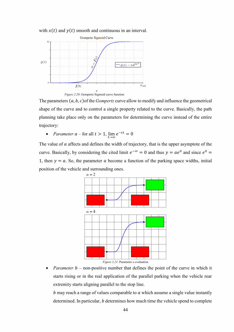
44

with 𝑥(𝑡) and 𝑦(𝑡) smooth and continuous in an interval.

The parameters (𝑎, 𝑏, 𝑐)of the Gompertz curve allow to modify and influence the geometrical

shape of the curve and to control a single property related to the curve. Basically, the path

planning take place only on the parameters for determining the curve instead of the entire

trajectory:

• Parameter 𝑎 – for all 𝑡 > 1, lim𝑡→∞

𝑒−𝑐𝑡 = 0

The value of 𝑎 affects and defines the width of trajectory, that is the upper asymptote of the

curve. Basically, by considering the cited limit 𝑒−∞ = 0 and thus 𝑦 = 𝑎𝑒0 and since 𝑒0 =

1, then 𝑦 = 𝑎. So, the parameter 𝑎 become a function of the parking space widths, initial

position of the vehicle and surrounding ones.

• Parameter 𝑏 – non-positive number that defines the point of the curve in which it

starts rising or in the real application of the parallel parking when the vehicle rear

extremity starts aligning parallel to the stop line.

𝑏 may reach a range of values comparable to 𝑎 which assume a single value instantly

determined. In particular, 𝑏 determines how much time the vehicle spend to complete

Figure 2.20: Gompertz Sigmoid curve function

Figure 2.21: Parameter a evaluation

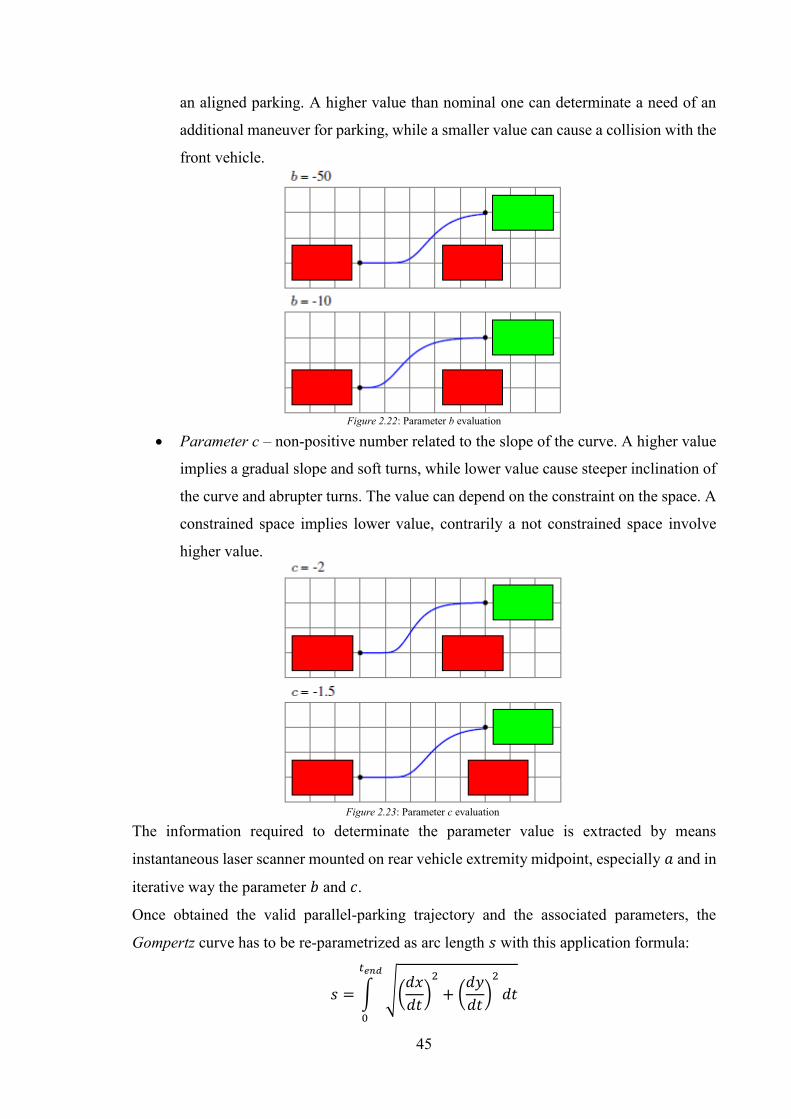
45

an aligned parking. A higher value than nominal one can determinate a need of an

additional maneuver for parking, while a smaller value can cause a collision with the

front vehicle.

• Parameter c – non-positive number related to the slope of the curve. A higher value

implies a gradual slope and soft turns, while lower value cause steeper inclination of

the curve and abrupter turns. The value can depend on the constraint on the space. A

constrained space implies lower value, contrarily a not constrained space involve

higher value.

The information required to determinate the parameter value is extracted by means

instantaneous laser scanner mounted on rear vehicle extremity midpoint, especially 𝑎 and in

iterative way the parameter 𝑏 and 𝑐.

Once obtained the valid parallel-parking trajectory and the associated parameters, the

Gompertz curve has to be re-parametrized as arc length 𝑠 with this application formula:

𝑠 = ∫ √(𝑑𝑥

𝑑𝑡)2

+ (𝑑𝑦

𝑑𝑡)2

𝑑𝑡

𝑡𝑒𝑛𝑑

0

Figure 2.22: Parameter b evaluation

Figure 2.23: Parameter c evaluation

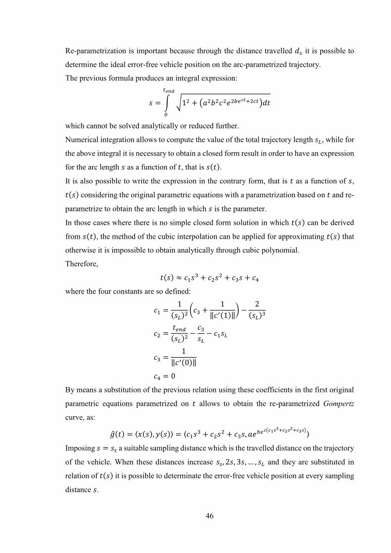
46

Re-parametrization is important because through the distance travelled 𝑑𝑠 it is possible to

determine the ideal error-free vehicle position on the arc-parametrized trajectory.

The previous formula produces an integral expression:

𝑠 = ∫ √12 + (𝑎2𝑏2𝑐2𝑒2𝑏𝑒𝑐𝑡+2𝑐𝑡)𝑑𝑡

𝑡𝑒𝑛𝑑

0

which cannot be solved analytically or reduced further.

Numerical integration allows to compute the value of the total trajectory length 𝑠𝐿, while for

the above integral it is necessary to obtain a closed form result in order to have an expression

for the arc length 𝑠 as a function of 𝑡, that is 𝑠(𝑡).

It is also possible to write the expression in the contrary form, that is 𝑡 as a function of 𝑠,

𝑡(𝑠) considering the original parametric equations with a parametrization based on 𝑡 and re-

parametrize to obtain the arc length in which 𝑠 is the parameter.

In those cases where there is no simple closed form solution in which 𝑡(𝑠) can be derived

from 𝑠(𝑡), the method of the cubic interpolation can be applied for approximating 𝑡(𝑠) that

otherwise it is impossible to obtain analytically through cubic polynomial.

Therefore,

𝑡(𝑠) ≈ 𝑐1𝑠3 + 𝑐2𝑠

2 + 𝑐3𝑠 + 𝑐4

where the four constants are so defined:

𝑐1 =1

(𝑠𝐿)2(𝑐3 +

1

‖𝑐′(1)‖) −

2

(𝑠𝐿)3

𝑐2 =𝑡𝑒𝑛𝑑(𝑠𝐿)2

−𝑐3𝑠𝐿− 𝑐1𝑠𝐿

𝑐3 =1

‖𝑐′(0)‖

𝑐4 = 0

By means a substitution of the previous relation using these coefficients in the first original

parametric equations parametrized on 𝑡 allows to obtain the re-parametrized Gompertz

curve, as:

��(𝑡) = ⟨𝑥(𝑠), 𝑦(𝑠)⟩ = ⟨𝑐1𝑠3 + 𝑐2𝑠

2 + 𝑐3𝑠, 𝑎𝑒𝑏𝑒𝑐(𝑐1𝑠

3+𝑐2𝑠2+𝑐3𝑠)⟩

Imposing 𝑠 = 𝑠𝑠 a suitable sampling distance which is the travelled distance on the trajectory

of the vehicle. When these distances increase 𝑠𝑠, 2𝑠, 3𝑠, … , 𝑠𝐿 and they are substituted in

relation of 𝑡(𝑠) it is possible to determinate the error-free vehicle position at every sampling

distance 𝑠.

47

The successive step is to find the tangent vector at each error-free position on the trajectory

and so, for a curve ��(𝑡|𝑠) parametrized by the parameter 𝑡 or arc length 𝑠, there exist a unit

tangent vector ��(𝑡|𝑠) such that:

��(𝑡|𝑠) =��′(𝑡|𝑠)

‖��′(𝑡|𝑠)‖

with ‖��(𝑡|𝑠)‖ = √𝑥′(𝑡|𝑠)2 + 𝑦′(𝑡|𝑠)2, where in this particular case are:

𝑥′(𝑠) = 3𝑐1𝑠2 + 2𝑐2𝑠 + 𝑐3

and

𝑦′(𝑠) = 𝑎𝑏𝑐𝑒𝑏𝑒𝑐(𝑐1𝑠

3+𝑐2𝑠2+𝑐3𝑠)

𝑒𝑐(𝑐1𝑠3+𝑐2𝑠

2+𝑐3𝑠) × (3𝑐1𝑠2 + 2𝑐2𝑠 + 𝑐3)

The unit tangent vector and the vehicle orientation has the same direction and the latter one

is strictly related to the orientation of the vehicle 𝜃 which can be determined at each position

based on 𝑠𝑠, 2𝑠, 3𝑠, … , 𝑠𝐿:

𝜃(𝑠)|𝑔𝑙𝑜𝑏𝑎𝑙 = 𝑎𝑡𝑎𝑛2 (��𝑦

��𝑥)

for ∀𝑠: 𝜃 ∈ [−180°, 180°] thanks to the sampling distance 𝑑𝑠. In this way the specific

orientation of the vehicle to achieve in order to realize the Gompertz trajectory in a single

maneuver is known.

The vehicle orientation is achieved by means the right magnitude of the steering angle (s)

determined by considering the dimension of the system and the trajectory curvature 𝑘:

𝑘(𝑠) =‖𝑔 ′(𝑠) × 𝑔 ′′(𝑠)‖

‖��′(𝑠)‖3

the necessary steering angle is

𝛾(𝑠) = 𝑎𝑡𝑎𝑛 ((𝐿(𝑦′′(𝑠)𝑥′(𝑠) − 𝑥′′(𝑠)𝑦′(𝑠))

‖��′(𝑠)‖3)

for all position in 𝑠.

The last step is the simulation of the vehicle motion through the vehicle model expression

on the found trajectory considering slip and determine if collisions will occur or not.

The entire process is shown and summarized in this figure where there is a simple

visualization of the optimal scheme result.

Figure 2.24: Visualization of the optimal scheme result

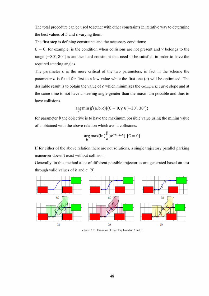
48

The total procedure can be used together with other constraints in iterative way to determine

the best values of 𝑏 and 𝑐 varying them.

The first step is defining constraints and the necessary conditions:

𝐶 = 0, for example, is the condition when collisions are not present and 𝛾 belongs to the

range [−30°, 30°] is another hard constraint that need to be satisfied in order to have the

required steering angles.

The parameter 𝑐 is the more critical of the two parameters, in fact in the scheme the

parameter 𝑏 is fixed for first to a low value while the first one (𝑐) will be optimized. The

desirable result is to obtain the value of 𝑐 which minimizes the Gompertz curve slope and at

the same time to not have a steering angle greater than the maximum possible and thus to

have collisions.

argcmin g′(a, b, c)|{C = 0, γ ∈[−30°, 30°]}

for parameter 𝑏 the objective is to have the maximum possible value using the minim value

of 𝑐 obtained with the above relation which avoid collisions:

argbmax(ln(

g

a )e−cminx)|{C = 0}

If for either of the above relation there are not solutions, a single trajectory parallel parking

maneuver doesn’t exist without collision.

Generally, in this method a lot of different possible trajectories are generated based on test

through valid values of 𝑏 and 𝑐. [9]

Figure 2.25: Evolution of trajectory based on b and c

49

CHAPTER 3

LATERAL DYNAMICS PROBLEM

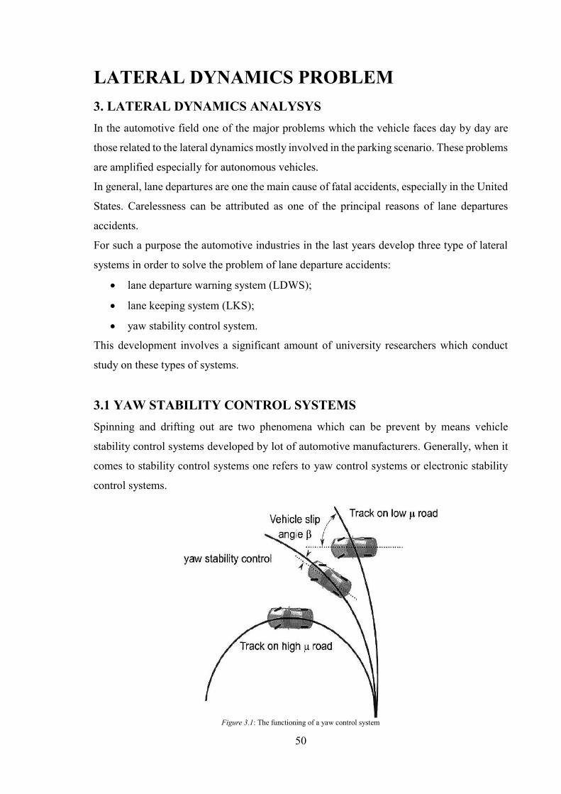
50

LATERAL DYNAMICS PROBLEM 3. LATERAL DYNAMICS ANALYSYS In the automotive field one of the major problems which the vehicle faces day by day are

those related to the lateral dynamics mostly involved in the parking scenario. These problems

are amplified especially for autonomous vehicles.

In general, lane departures are one the main cause of fatal accidents, especially in the United

States. Carelessness can be attributed as one of the principal reasons of lane departures

accidents.

For such a purpose the automotive industries in the last years develop three type of lateral

systems in order to solve the problem of lane departure accidents:

• lane departure warning system (LDWS);

• lane keeping system (LKS);

• yaw stability control system.

This development involves a significant amount of university researchers which conduct

study on these types of systems.

3.1 YAW STABILITY CONTROL SYSTEMS Spinning and drifting out are two phenomena which can be prevent by means vehicle

stability control systems developed by lot of automotive manufacturers. Generally, when it

comes to stability control systems one refers to yaw control systems or electronic stability

control systems.

Figure 3.1: The functioning of a yaw control system

51

The lower curve of the figure shows the desirable trajectory to follow as response of a

steering input come from the driver in dry-road condition and high tire-road friction

coefficient. In this specific case it is possible to obtain the required lateral force due to the e

high friction coefficient which allows to approach the curved road. The upper curve shows

as in cases in which the friction coefficient is small, or the vehicle speed is too high, the is

uncapable to follow the nominal motion required and it will travel on a larger radius

trajectory and so there will be a smaller curvature.

The expected nominal motion requested by the driver can be respected if the yaw control

system become able to restore the right yaw velocity of the vehicle. The objective is to obtain

the maximum result closer to the expected nominal yaw rate even if once can be in not

favorable situation like in low friction coefficient scenario.

In the last ten years many automotive industries carried on several study about yaw control

system to develop through vehicle experiment and simulations.

The main types of stability control system which the companies have been proposed and

developed to solve the yaw dynamics control problem are three and they are the following

ones:

• differential braking systems, which is a system that use the ABS braking system on

the vehicle for applying differential braking between the right and left wheels in order

to control the yaw moment;

• steer-by-wire systems, which acts on the driver’s steering angle input by adding if

needed a correction on the angle to the wheels;

• active torque distribution systems, which use an active differentials and all-wheel

drive to control in independent way the drive torque distributed to each wheel and

then supply an active control of both yam moment and traction.

3.2 KINEMATIC MODEL OF LATERAL VEHICLE MOTION A mathematical description of the vehicle motion without putting into play the forces which

affect the motion can be developed. The equations will be based only on geometric

relationships which act on the system.

A bicycle model is the most important used model to describe and approximate the vehicle

motion. In this model the four wheels of the vehicle are placed by one single wheel for each

wheel couple (rear and front) of the first one at two points, A and B.

52

The rear steering angle 𝛿𝑟 and the front one 𝛿𝑓 are associated to a system in which we assume

that both wheels can be steered with the front only steering and the rear one can be set to

zero. The point C is the centre of gravity of the vehicle and the distance points between A or

B and C are 𝑙𝑓 and 𝑙𝑟 respectively. The vehicle wheelbase is 𝐿 = 𝑙𝑓 + 𝑙𝑟.

Under the assumption of planar motion of the vehicle, it is defined a three-coordinate system

(𝑋, 𝑌, 𝜓) to describe its motion. The first two coordinates (𝑋, 𝑌) are inertial coordinates of

the centre of gravity location of the vehicle, while 𝜓 is the heading angle of the vehicle and

it is associated to the vehicle orientation and 𝑉 denote the vehicle velocity at the c.g. The

angle that makes the vehicle with respect to the longitudinal axes is the slip angle which is

defined with the variable 𝛽.

The velocity vectors at the points A and B are in the direction of the orientation of both

wheels (front and rear) and it is the main assumption on the kinematic model development.

The velocity vector at the front wheel produce an angle 𝛿𝑓 with the longitudinal axis, while

the one at the real wheel make an angle 𝛿𝑟 with the longitudinal axes, that corresponds to

assume the slip angle equals to zero at both wheels (reasonable assumption for low speed

motion of the vehicle). The lateral force generated by the tires is small at low speeds.

Generally, the total lateral force from both tires to drive on any circular 𝑅 radius road is:

𝑚𝑉2

𝑅

which varies in quadratic form with the speed and it becomes obviously small at low speed.

When the lateral forces are small it is necessary to assume that the velocity vector is in

direction of the wheel at each wheel.

Figure 3.2: Kinematics of lateral vehicle motion

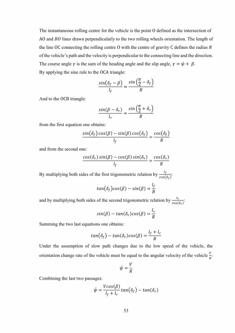
53

The instantaneous rolling centre for the vehicle is the point O defined as the intersection of

AO and 𝐵𝑂 lines drawn perpendicularly to the two rolling wheels orientation. The length of

the line OC connecting the rolling centre O with the centre of gravity C defines the radius 𝑅

of the vehicle’s path and the velocity is perpendicular to the connecting line and the direction.

The course angle 𝛾 is the sum of the heading angle and the slip angle, 𝛾 = 𝜓 + 𝛽.

By applying the sine rule to the OCA triangle:

𝑠𝑖𝑛(𝛿𝑓 − 𝛽)

𝑙𝑓=𝑠𝑖𝑛 (

𝜋2 − 𝛿𝑓)

𝑅

And to the OCB triangle:

𝑠𝑖𝑛(𝛽 − 𝛿𝑟)

𝑙𝑟=𝑠𝑖𝑛 (

𝜋2 + 𝛿𝑟)

𝑅

from the first equation one obtains:

𝑠𝑖𝑛(𝛿𝑓) 𝑐𝑜𝑠(𝛽) − 𝑠𝑖𝑛(𝛽) 𝑐𝑜𝑠(𝛿𝑓)

𝑙𝑓=𝑐𝑜𝑠(𝛿𝑓)

𝑅

and from the second one:

𝑐𝑜𝑠(𝛿𝑟) 𝑠𝑖𝑛(𝛽) − 𝑐𝑜𝑠(𝛽) 𝑠𝑖𝑛(𝛿𝑟)

𝑙𝑓=𝑐𝑜𝑠(𝛿𝑟)

𝑅

By multiplying both sides of the first trigonometric relation by 𝑙𝑓

𝑐𝑜𝑠(𝛿𝑓):

𝑡𝑎𝑛(𝛿𝑓)𝑐𝑜𝑠(𝛽) − 𝑠𝑖𝑛(𝛽) =𝑙𝑓

𝑅

and by multiplying both sides of the second trigonometric relation by 𝑙𝑟

𝑐𝑜𝑠(𝛿𝑟):

𝑠𝑖𝑛(𝛽) − 𝑡𝑎𝑛(𝛿𝑟)𝑐𝑜𝑠(𝛽) =𝑙𝑟𝑅

Summing the two last equations one obtains:

𝑡𝑎𝑛(𝛿𝑓) − 𝑡𝑎𝑛(𝛿𝑟)𝑐𝑜𝑠(𝛽) =𝑙𝑓 + 𝑙𝑟

𝑅

Under the assumption of slow path changes due to the low speed of the vehicle, the

orientation change rate of the vehicle must be equal to the angular velocity of the vehicle 𝑉𝑅:

�� =𝑉

𝑅

Combining the last two passages:

�� =𝑉𝑐𝑜𝑠(𝛽)

𝑙𝑓 + 𝑙𝑟𝑡𝑎𝑛(𝛿𝑓) − 𝑡𝑎𝑛(𝛿𝑟)

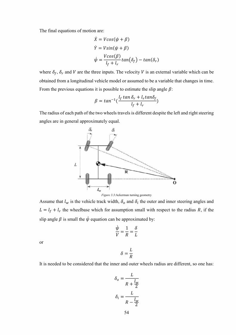
54

The final equations of motion are:

�� = 𝑉𝑐𝑜𝑠(𝜓 + 𝛽)

�� = 𝑉𝑠𝑖𝑛(𝜓 + 𝛽)

�� =𝑉𝑐𝑜𝑠(𝛽)

𝑙𝑓 + 𝑙𝑟𝑡𝑎𝑛(𝛿𝑓) − 𝑡𝑎𝑛(𝛿𝑟)

where 𝛿𝑓, 𝛿𝑟 and 𝑉 are the three inputs. The velocity 𝑉 is an external variable which can be

obtained from a longitudinal vehicle model or assumed to be a variable that changes in time.

From the previous equations it is possible to estimate the slip angle 𝛽:

𝛽 = 𝑡𝑎𝑛−1(𝑙𝑓 𝑡𝑎𝑛 𝛿𝑟 + 𝑙𝑟𝑡𝑎𝑛𝛿𝑓

𝑙𝑓 + 𝑙𝑟)

The radius of each path of the two wheels travels is different despite the left and right steering

angles are in general approximately equal.

Assume that 𝑙𝑤 is the vehicle track width, 𝛿𝑜 and 𝛿𝑖 the outer and inner steering angles and

𝐿 = 𝑙𝑓 + 𝑙𝑟 the wheelbase which for assumption small with respect to the radius 𝑅, if the

slip angle 𝛽 is small the �� equation can be approximated by:

𝜓

𝑉

=1

𝑅=𝛿

𝐿

or

𝛿 =𝐿

𝑅

It is needed to be considered that the inner and outer wheels radius are different, so one has:

𝛿𝑜 =𝐿

𝑅 +𝑙𝑤2

𝛿𝑖 =𝐿

𝑅 −𝑙𝑤2

Figure 3.3:Ackerman turning geometry

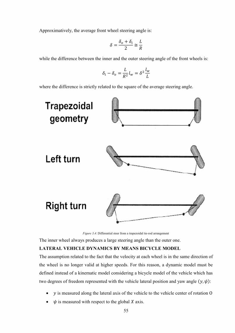
55

Approximatively, the average front wheel steering angle is:

𝛿 =𝛿𝑜 + 𝛿𝑖2

≅𝐿

𝑅

while the difference between the inner and the outer steering angle of the front wheels is:

𝛿𝑖 − 𝛿𝑜 =𝐿

𝑅2𝑙𝑤 = 𝛿

2𝑙𝑤𝐿

where the difference is strictly related to the square of the average steering angle.

The inner wheel always produces a large steering angle than the outer one.

LATERAL VEHICLE DYNAMICS BY MEANS BICYCLE MODEL

The assumption related to the fact that the velocity at each wheel is in the same direction of

the wheel is no longer valid at higher speeds. For this reason, a dynamic model must be

defined instead of a kinematic model considering a bicycle model of the vehicle which has

two degrees of freedom represented with the vehicle lateral position and yaw angle (𝑦, 𝜓):

• 𝑦 is measured along the lateral axis of the vehicle to the vehicle center of rotation O

• 𝜓 is measured with respect to the global 𝑋 axis.

Figure 3.4: Differential steer from a trapezoidal tie-rod arrangement

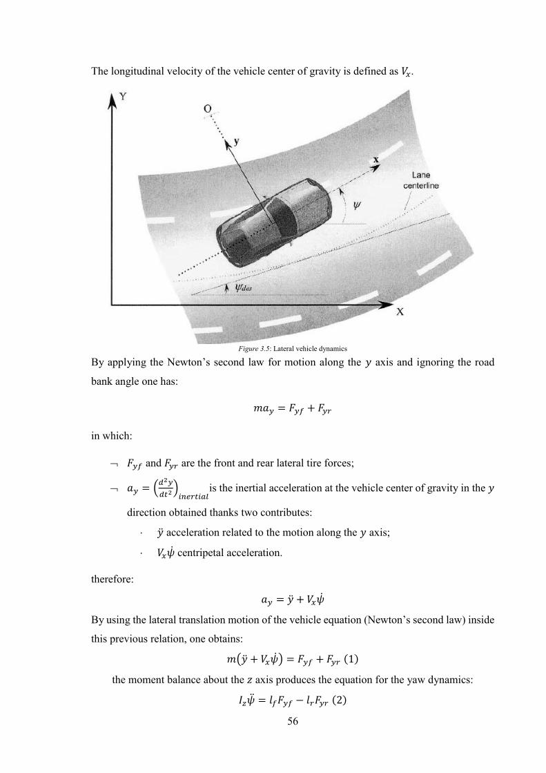
56

The longitudinal velocity of the vehicle center of gravity is defined as 𝑉𝑥.

By applying the Newton’s second law for motion along the 𝑦 axis and ignoring the road

bank angle one has:

𝑚𝑎𝑦 = 𝐹𝑦𝑓 + 𝐹𝑦𝑟

in which:

𝐹𝑦𝑓 and 𝐹𝑦𝑟 are the front and rear lateral tire forces;

𝑎𝑦 = (𝑑2𝑦

𝑑𝑡2)𝑖𝑛𝑒𝑟𝑡𝑖𝑎𝑙

is the inertial acceleration at the vehicle center of gravity in the 𝑦

direction obtained thanks two contributes:

�� acceleration related to the motion along the 𝑦 axis;

𝑉𝑥�� centripetal acceleration.

therefore:

𝑎𝑦 = �� + 𝑉𝑥��

By using the lateral translation motion of the vehicle equation (Newton’s second law) inside

this previous relation, one obtains:

𝑚(�� + 𝑉𝑥��) = 𝐹𝑦𝑓 + 𝐹𝑦𝑟 (1)

the moment balance about the 𝑧 axis produces the equation for the yaw dynamics:

𝐼𝑧�� = 𝑙𝑓𝐹𝑦𝑓 − 𝑙𝑟𝐹𝑦𝑟 (2)

Figure 3.5: Lateral vehicle dynamics

57

The next step is dedicated for modelling the lateral tire forces 𝐹𝑦𝑓 and 𝐹𝑦𝑟 that act on the

vehicle, which are proportional to the slip angle when it is small. The slip angle of a tire is

the angle between the tire orientation and the velocity vector of the wheel orientation:

The front slip angle is:

𝛼𝑓 = 𝛿 − 𝜃𝑣𝑓

where 𝛿 is the front wheel steering angle, while 𝜃𝑣𝑓 is the angle between the vector velocity

direction and the longitudinal axis of the vehicle, the front tire velocity angle.

Similarly, the rear slip angle is:

𝛼𝑟 = −𝜃𝑣𝑟

where 𝜃𝑣𝑟 is the rear tire velocity angle.

The slip angle results zero when the vehicle travels straight ahead and is not steering and so,

the two components of the slip angle are both zero.

In the static region of the contact zone, there is a contact of the tip of each tread with the

ground and this remains stationary. So, the top of the tread moving with respect to the tread

tip causes a tread deformation. If one denotes the velocity at the wheel as 𝑉𝑤, the lateral

component of the velocity is 𝑉𝑤 𝑠𝑖𝑛(𝛼). The magnitude of the tread lateral deflection is

proportional both to the lateral velocity and to the amount of time spent by the tread in the

contact zone. Finally, the lateral tread deflection is proportional only to the slip angle.

Figure 3.6: Tire slip angle

58

The lateral tire force on the tire is strictly related and proportional to the magnitude of lateral

deflection of the treads in the contact zone, while for small slip angles it is proportional to

the slip angle.

Given these considerations, it is possible to define the lateral tire force for the front wheels

of the vehicle:

𝐹𝑦𝑓 = 𝐶𝛼(𝛿 − 𝜃𝑣𝑓)

in which 𝐶𝛼 is denoted as cornering stiffness and it is a proportionality constant.

Similarly, for the rear wheels of the vehicle it is definable the lateral tire force:

𝐹𝑦𝑟 = 𝐶𝛼(−𝜃𝑣𝑟)

where also in this case 𝐶𝛼 is the cornering stiffness.

The lateral and longitudinal velocity ratio at each wheel is useful to calculate the velocity

angle at that wheel by exploiting these two relations to determinate 𝜃𝑣𝑓 and 𝜃𝑣𝑟:

𝑡𝑎𝑛(𝜃𝑣𝑓) =𝑉𝑦 + 𝑙𝑓��

𝑉𝑥

𝑡𝑎𝑛(𝜃𝑣𝑟) =𝑉𝑦 − 𝑙𝑟��

𝑉𝑥

with 𝑉𝑦 and 𝑉𝑥 lateral and longitudinal velocity at the center of gravity of the vehicle, �� yaw

rate of the vehicle and 𝑙𝑟 and 𝑙𝑓 longitudinal distances from center of gravity to the rear and

front wheels respectively.

Under the assumption of small angle:

𝜃𝑣𝑓 =𝑉𝑦 + 𝑙𝑓��

𝑉𝑥

𝜃𝑣𝑟 =𝑉𝑦 − 𝑙𝑟��

𝑉𝑥

Thus,

𝐹𝑦𝑓 = 𝐶𝛼 (𝛿 −𝑉𝑦 + 𝑙𝑓��

𝑉𝑥)

𝐹𝑦𝑟 = 𝐶𝛼 (−𝑉𝑦 − 𝑙𝑟��

𝑉𝑥)

Definitely, starting from the (1) and (2) relations

{𝑚(�� + ��𝑉𝑥) = 𝐹𝑦𝑓 + 𝐹𝑦𝑟

𝐼𝑧�� = 𝑙𝑓𝐹𝑦𝑓 − 𝑙𝑟𝐹𝑦𝑟

59

Denoting �� as 𝑉��, using the tire forces relations and the inverse relation of the front and rear

tire velocity angle:

𝐹𝑦𝑓 = 𝐶𝛼(𝛿 − 𝜃𝑣𝑓)

𝐹𝑦𝑟 = 𝐶𝛼(−𝜃𝑣𝑟)

𝜃𝑣𝑓 = tan−1 (𝑉𝑦 − 𝑙𝑟��

𝑉𝑥)

𝜃𝑣𝑟 = tan−1 (𝑉𝑦 − 𝑙𝑟��

𝑉𝑥)

one obtains:

{𝑚(𝑉�� + ��𝑉𝑥) = 𝐹𝑦𝑓 + 𝐹𝑦𝑟

𝐼𝑧�� = 𝑙𝑓𝐹𝑦𝑓 − 𝑙𝑟𝐹𝑦𝑟

that is:

{

𝑉�� =1

𝑚(−𝑉𝑥�� + 𝐹𝑦𝑓 + 𝐹𝑦𝑟)

�� =1

𝐼𝑧(𝑙𝑓𝐹𝑦𝑓 − 𝑙𝑟𝐹𝑦𝑟)

which is at last:

{

𝑉�� =

1

𝑚(−𝑉𝑥�� + 𝐶𝛼 [𝛿 − tan

−1 (𝑉𝑦 + 𝑙𝑓��

𝑉𝑥)] − 𝐶𝛼 [tan

−1 (𝑉𝑦 − 𝑙𝑟��

𝑉𝑥)])

�� =1

𝐼𝑧(𝑙𝑓𝐶𝛼 [𝛿 − tan

−1 (𝑉𝑦 + 𝑙𝑓��

𝑉𝑥)] − 𝑙𝑟𝐶𝛼 [tan

−1 (𝑉𝑦 − 𝑙𝑟��

𝑉𝑥)])

the final nonlinear vehicle model.

The main idea when there is an approach to a nonlinear model is that to “convert” it in a

correspondent linearize one.

In this regard, in the next chapter there is an explanation on how a nonlinear system can be

traduced in a linear one. [10]

60

CHAPTER 4

LINEARIZATION OF NONLINEAR SYSTEMS

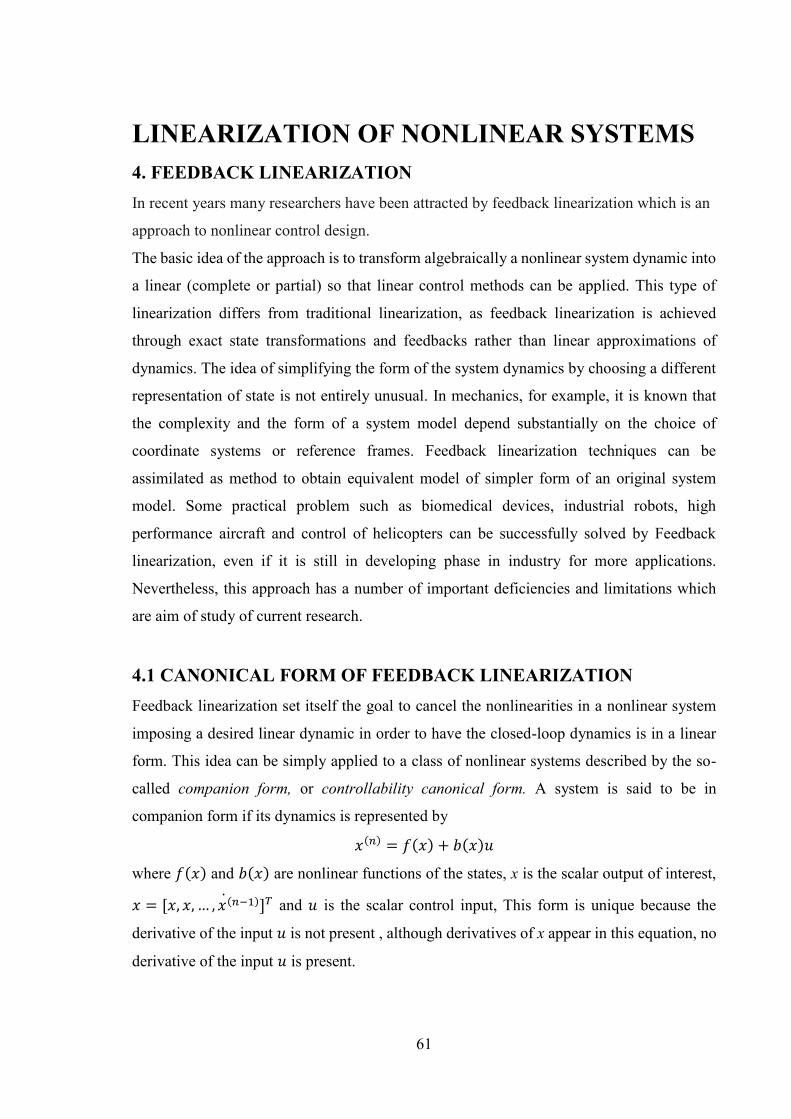
61

LINEARIZATION OF NONLINEAR SYSTEMS 4. FEEDBACK LINEARIZATION In recent years many researchers have been attracted by feedback linearization which is an

approach to nonlinear control design.

The basic idea of the approach is to transform algebraically a nonlinear system dynamic into

a linear (complete or partial) so that linear control methods can be applied. This type of

linearization differs from traditional linearization, as feedback linearization is achieved

through exact state transformations and feedbacks rather than linear approximations of

dynamics. The idea of simplifying the form of the system dynamics by choosing a different

representation of state is not entirely unusual. In mechanics, for example, it is known that

the complexity and the form of a system model depend substantially on the choice of

coordinate systems or reference frames. Feedback linearization techniques can be

assimilated as method to obtain equivalent model of simpler form of an original system

model. Some practical problem such as biomedical devices, industrial robots, high

performance aircraft and control of helicopters can be successfully solved by Feedback

linearization, even if it is still in developing phase in industry for more applications.

Nevertheless, this approach has a number of important deficiencies and limitations which

are aim of study of current research.

4.1 CANONICAL FORM OF FEEDBACK LINEARIZATION Feedback linearization set itself the goal to cancel the nonlinearities in a nonlinear system

imposing a desired linear dynamic in order to have the closed-loop dynamics is in a linear

form. This idea can be simply applied to a class of nonlinear systems described by the so-

called companion form, or controllability canonical form. A system is said to be in

companion form if its dynamics is represented by

𝑥(𝑛) = 𝑓(𝑥) + 𝑏(𝑥)𝑢

where 𝑓(𝑥) and 𝑏(𝑥) are nonlinear functions of the states, x is the scalar output of interest,

𝑥 = [𝑥, 𝑥, … , 𝑥(𝑛−1)] 𝑇 and 𝑢 is the scalar control input, This form is unique because the

derivative of the input 𝑢 is not present , although derivatives of x appear in this equation, no

derivative of the input 𝑢 is present.

62

The state-space representation of the equation can be written in this way:

𝑑

𝑑𝑡[

𝑥1…𝑥𝑛−1𝑥𝑛

] = [

𝑥2…𝑥𝑛

𝑓(𝑥) + 𝑏(𝑥)𝑢

]

Using the control input (assuming b to be non-zero):

𝑢 ≈1

𝑏[𝑣 − 𝑓]

for all those systems which can be expressed in the controllability canonical form, it is

possible to cancel the nonlinearities obtaining the simple input-output relation:

𝑥(𝑛) = 𝑣

Then, the control law:

𝑣 = −𝑘0 − 𝑘1�� − ⋯ .−𝑘𝑛−1𝑥(𝑛−1)

with the 𝑘𝑖 chosen so that the polynomial 𝑝𝑛 + 𝑘𝑛−1𝑝𝑛−1 +⋯ .+𝑘0 has all its roots strictly

in the left-half complex plane, leads to the exponentially stable dynamics which implies that

𝑥(𝑡) → 0. For tasks involving the tracking of a desired output 𝑥𝑑(𝑡), the control law:

𝑣 = 𝑥𝑑(𝑛) − 𝑘0𝑒 − 𝑘1�� − ⋯ .−𝑘𝑛−1𝑒

(𝑛−1)

(where the tracking error is 𝑒(𝑡) = 𝑥(𝑡) − 𝑥𝑑(𝑡) is the tracking error) leads to exponentially

convergent tracking.

When the system has a nonlinear dynamic, which is not in a controllability canonical form,

it is important to use algebraic transformations to have the dynamics into the controllabity

form before using the feedback linearization design or to exploit partial linearization of the

original system dynamics, instead of full linearization.

4.2 INPUT-STATE LINEARIZATION Considering the problem of control input design for a single-input 𝑢 nonlinear system of the

form:

�� = 𝑓(𝑥, 𝑢)

this problem can be solved in two steps thanks to the input-state linearization technique:

1. finds a state transformation 𝑧 = 𝑧(𝑥) and an input transformation 𝑢 = 𝑢(𝑥, 𝑣) in

order to transform the nonlinear system dynamics into an equivalent linear time-

invariant dynamic in the form �� = 𝐴𝑧 + 𝑏𝑣;

2. design 𝑣 using standard linear techniques.

63

The closed-loop system under the control law obtained is represented in this block diagram:

In this control loop two loops with two different functions are detected:

➢ the inner loop for the linearization of the input-state relation;

➢ the outer loop for the stabilization of the closed-loop dynamics.

4.3 INPUT-OUTPUT LINEARIZATION For this type of linearization, it is possible consider the tracking control problem and in

particular the system:

�� = 𝑓(𝑥, 𝑢)

𝑦 = ℎ(𝑥)

and with the assumption that the objective is to make sure that the output 𝑦(𝑡) track a desired

trajectory 𝑦𝑑(𝑡) while keeping the whole state bounded, where 𝑦𝑑(𝑡) its time derivatives

until a sufficiently high order are assumed to be known and bounded. One difficulty

associated with this model is that the output 𝑦 is only indirectly related to the input 𝑢, by the

state variable 𝑥 and the nonlinear state equations.

Thus, the design of the input 𝑢 for the control of the output 𝑦 start to be complicated even if

the difficulty can be reduced to the research of a simple and explicit relationship between

the control input 𝑢 and the system output 𝑦. To generate a direct relation between the output

𝑦 and the input 𝑢, it is necessary to differentiate the output until the relation is found. If we

require to differentiate r times the output of the system, it is said that the systems have

relative degree 𝑟 (in linear system coincides with the excess of poles over zeros). It is

possible take at most 𝑛 differentiations of the output 𝑦 to make appear the input 𝑢, 𝑟 ≤ 𝑛. If

the 𝑛 differentiations are exceeded, and the control input never appeared, the system would

be of order higher than 𝑛 and not controllable.

In the input-output linearization a part of the system dynamics called internal dynamics

seems “unobservable”, because it cannot be seen from the external input-output relation. If

the internal dynamics is stable, the tracking control design problem can be solved.

Figure 4.1: Closed-loop system

64

Moreover, the input-output linearization can be applied also on the stabilization problem as

well as the output tracking.

In stabilization problems:

1. there is no reason to limit the choice of the output 𝑦 = ℎ(𝑥) to be a physically

important quantity (in tracking problems the physical task determines the choice of

output). To generate a linear relation input-output it is possible exploit an artificial

output using any function of x.

2. different choices of output function allow to obtain different internal dynamics.

One choice of output can lead to a stable internal dynamic (or no internal dynamics),

while another one leads to having an unstable one. The best choice is the output

function which guarantees an associated stable internal dynamic.

A particular case is when the order of the system is the same as the system relative degree 𝑟,

that is when 𝑛 differentiations are applied on the output 𝑦 to obtain a linear input-output

relation. In this case, the variables 𝑦, ��, … , 𝑦(𝑛−1) becomes the new state variables for the

system and thus, the consequences are that there is no internal dynamics associated with this

input-output linearization that in particular leads to input-state linearization, and both state

regulation and output tracking (for the particular output) can be achieved easily.

4.4 THE INTERNAL DYNAMICS OF LINEAR SYSTEM In general, to direct determine the stability of the internal dynamics is very difficult because

it is nonlinear, non-autonomous and coupled to the “external” closed-loop dynamics. The

objective for the internal dynamics is finding the simpler ways for determining its stability.

By evaluating two apparently similar linear systems, but with an associated transfer function

that differs exclusively for zeros (equal poles), it is possible to notice how a tracking design

method is applicable only in one of the two cases. In particular, the design is successful in

the case of the transfer function with left half-plane zero, but fails in the case of the function

with right half-plane zero. From here it is inferred that the internal dynamics is stable if the

plant is "minimum-phase", that is in the left half-plane and this is applicable to all linear

systems. As for the "non-minimum phase" systems, a perfect tracking of arbitrary trajectories

requires infinite control effort.

For summarize, if the systems are phase minimum, then with the zeros in the left-half plane,

this will imply that the internal dynamics are stable regardless of the magnitudes of the

desired 𝑦, … , 𝑦(𝑟) (with 𝑟 relative degree) and of the initial conditions.

65

4.5 THE ZERO-DYNAMICS One important aspect to be considered is how to determine the stability of the internal

dynamics in the case of nonlinear system. Since for linear system this stability depends on

the locations of the zeros, it is necessary as first requirement to extend the notion of zeros in

order to understand this concept in the nonlinear case. For nonlinear system, transfer function

cannot be defined. In particular, zeros are intrinsic properties of linear plant systems, while

the stability of the internal dynamics for nonlinear systems depends on the specific control

input. For nonlinear systems a way to treat these difficulties is to define a so called zero-

dynamics that are the internal dynamics of the system when the input keeps the systems

output at zero. The zero-dynamics become an intrinsic feature for nonlinear systems, which

is independent from the desired trajectories or the chosen control law. The result is general

for linear systems, in particular the global asymptotic stability of the zero-dynamics is

guaranteed when the systems has all zeros in the left-half plane and implies the global

stability of the internal dynamics.

In case of nonlinear system, in stabilization problem, the local stability of the zero-dynamics

guarantees the local stability of the internal dynamics, while in tracking problem this relation

for the global stability doesn’t exist.

Definitely, to examine the local stability of the zero-dynamics may be much easier and

simpler than evaluating the internal dynamics stability, because only the internal states are

relating to the zero-dynamics, while the internal dynamics is linked in some way to the

desired trajectories and the external dynamics.

The control design method based on input-output linearization can be summarized in three

steps:

1. differentiate the output 𝑦 until the input appears;

2. choose the input 𝑢 in order to guarantee the tracking convergence, but most of all to

cancel the nonlinearities;

3. stability study of the internal dynamics.

For what concerns the topology the input-output linearization, it is possible to outline in the

following way:

➢ if 𝑟 = 𝑛, then the nonlinear system is fully linearized, and the procedure allows to

have a satisfactory controller

➢ if 𝑟 < 𝑛, then the nonlinear systems are partly linearized, and the controller can be

applied based on the stability of the internal dynamics.

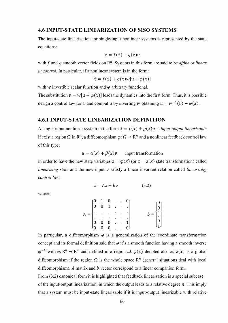
66

4.6 INPUT-STATE LINEARIZATION OF SISO SYSTEMS The input-state linearization for single-input nonlinear systems is represented by the state

equations:

�� = 𝑓(𝑥) + 𝑔(𝑥)𝑢

with 𝑓 and 𝑔 smooth vector fields on R𝑛. Systems in this form are said to be affine or linear

in control. In particular, if a nonlinear system is in the form:

�� = 𝑓(𝑥) + 𝑔(𝑥)𝑤[𝑢 + 𝜑(𝑥)]

with 𝑤 invertible scalar function and 𝜑 arbitrary functional.

The substitution 𝑣 = 𝑤[𝑢 + 𝜑(𝑥)] leads the dynamics into the first form. Thus, it is possible

design a control law for 𝑣 and comput 𝑢 by inverting 𝑤 obtaining 𝑢 = 𝑤−1(𝑣) − 𝜑(𝑥).

4.6.1 INPUT-STATE LINEARIZATION DEFINITION A single-input nonlinear system in the form �� = 𝑓(𝑥) + 𝑔(𝑥)𝑢 is input-output linearizable

if exist a region in R𝑛, a diffeomorphism 𝜑: → R𝑛 and a nonlinear feedback control law

of this type: 𝑢 = 𝛼(𝑥) + 𝛽(𝑥)𝑣 input transformation

in order to have the new state variables 𝑧 = 𝜑(𝑥) (or 𝑧 = 𝑧(𝑥) state transformation) called

linearizing state and the new input 𝑣 satisfy a linear invariant relation called linearizing

control law:

�� = 𝐴𝑧 + 𝑏𝑣 (3.2)

where:

𝐴 =

[ 0 1 0 . . 00 0 1 . . .. . . . . .. . . . . .0 0 0 . . 10 0 0 . . 0]

𝑏 =

[ 00..01]

In particular, a diffeomorphism 𝜑 is a generalization of the coordinate transformation

concept and its formal definition said that 𝜑 it’s a smooth function having a smooth inverse

𝜑−1 with 𝜑: R𝑛 → R𝑛 and defined in a region 𝜑(𝑥) denoted also as 𝑧(𝑥) is a global

diffeomorphism if the region is the whole space R𝑛 (general situations deal with local

diffeomorphism). 𝐴 matrix and 𝑏 vector correspond to a linear companion form.

From (3.2) canonical form it is highlighted that feedback linearization is a special subcase

of the input-output linearization, in which the output leads to a relative degree 𝑛. This imply

that a system must be input-state linearizable if it is input-output linearizable with relative

67

degree 𝑛. Nevertheless, there is a relationship between the input-state linearization and input-

output linearization according to which a nonlinear system is input-state linearizable if, and

only if, the first new state 𝑧1(x) which represents the output in the case of input-state

linearization.

Furthermore, a nonlinear system with 𝑓(𝑥) and 𝑔(𝑥) smooth vector fields, is input-state

linearizable if, and only if, a region exists such that the following conditions are respected:

• {𝑔, 𝑎𝑑𝑓𝑔,… , 𝑎𝑑𝑓𝑛−1𝑔} vector fields are linearly independent in

• {𝑔, 𝑎𝑑𝑓𝑔,… , 𝑎𝑑𝑓𝑛−2𝑔} set is involutive in

The first condition is almost a reinterpretation of a simply controllability condition for

nonlinear system (for linear systems the vector fields are {𝑏, 𝐴𝑏, … , 𝐴𝑛−1𝑏} and the

independence corresponds to the invertibility of the controllability matrix). The second

condition is not generally satisfied and in particular, a linearly independent set of vector

fields is said to be involutive if, and only if, there are a scalar function 𝛼𝑖𝑗𝑘: R𝑛 → R such

that:

[𝑓𝑖 , 𝑓𝑗] = ∑𝛼𝑖𝑗𝑘(𝑥)𝑓𝑘(𝑥)

𝑛

𝑘=1

∀𝑖, 𝑗

A condition of integrability derives from that of involutivity (necessity and sufficiency).

Obviously, it is needed to define the adjoint that is a vector fields also known as Lie bracket.

Particularly, starting from two vector fields 𝑓 and 𝑔 on R𝑛, the Lie bracket of 𝑓 and 𝑔 will

be the third vector field determined by:

[𝑓, 𝑔] = ∇𝑔 𝑓 − ∇𝑓 𝑔

commonly written as 𝑎𝑑𝑓𝑔 (where 𝑎𝑑 stands for “adjoint”). By repeating Lie brackets it is

defined recursively cases of this type:

𝑎𝑑𝑓0𝑔 = 𝑔

𝑎𝑑𝑓𝑖𝑔 = [𝑓, 𝑎𝑑𝑓𝑖−1𝑔] for 𝑖 = 1,2, …

Lie brackets benefit of the following proprieties:

1. biliniearity:

[𝛼1𝑓1 + 𝛼2𝑓2, 𝑔] = 𝛼1[𝑓1, 𝑔] + 𝛼2[𝑓2, 𝑔]

[𝑓1, 𝛼1𝑔1 + 𝛼2𝑔2] = 𝛼1[𝑓, 𝑔1] + 𝛼2[𝑓, 𝑔2]

where 𝑓, 𝑓1, 𝑓2, 𝑔, 𝑔1 , 𝑔2 are vector fields, while 𝛼1 and 𝛼2 are constant scalars.

2. skew-commutativity:

[𝑓, 𝑔] = −[𝑔, 𝑓]

68

3. Jacobi Identity:

𝐿𝑎𝑑𝑓𝑔ℎ = 𝐿𝑓𝐿𝑔ℎ − 𝐿𝑔𝐿𝑓ℎ

where ℎ(𝑥) is a smooth scalar funcion of 𝑥 and 𝐿𝑓 and the others are the Lie derivates

explained in the next paragraph.

4.7.1.1 HOW TO PERFORM INPUT-STATE LINEARIZATION Input-state linearization of a nonlinear system is divided in four following steps:

• construction of the vector fields 𝑔, 𝑎𝑑𝑓𝑔,… , 𝑎𝑑𝑓𝑛−1𝑔 for the given system;

• controllability and involutivity conditions verification;

• if both conditions are satisfied, it is needed to find the new output function 𝑧1 related

to the input-output linearization of relative degree 𝑛:

∇𝑧1𝑎𝑑𝑓𝑖 𝑔 = 0 𝑖 = 0,… , 𝑛 − 2

∇𝑧1𝑎𝑑𝑓𝑛−1 𝑔 ≠ 0

• state transformation 𝑧(𝑥) = [𝑧1 𝐿𝑓 𝑧1 … 𝐿𝑓𝑛−1 𝑧1]𝑇 and input transformation

computation:

𝛼(𝑥) = −𝐿𝑓𝑛 𝑧1

𝐿𝑔 𝐿𝑓𝑛−1 𝑧1

𝛽(𝑥) =1

𝐿𝑔 𝐿𝑓𝑛−1 𝑧1

With the transformed state equation into a linear form, it is possible design controllers for

either tracking problems or stabilization purposes.

The scalar function 𝐿𝑓ℎ called Lie derivative (or simply, the derivative) of a generic scalar

function ℎ(𝑥): R𝑛 → R with respect to a vector field 𝑓(𝑥): R𝑛 → R𝑛. The Lie derivative of

ℎ with respect to 𝑓 is a scalar function defined by 𝐿𝑓ℎ = ∇ℎ 𝑓.

Therefore, the Lie derivative 𝐿𝑓ℎ is the directional derivative of ℎ along the vector 𝑓

direction, which has this property:

𝐿𝑓0ℎ = ℎ 𝐿𝑓𝑖ℎ = 𝐿𝑓(𝐿𝑓𝑖−1ℎ) = ∇(𝐿𝑓𝑖−1ℎ)𝑓 for 𝑖 = 1,2, ….

𝐿𝑔𝐿𝑓ℎ = ∇(𝐿𝑓ℎ)𝑔

[11]

69

CHAPTER 5

SYSTEM CONTROL DESIGN

70

SYSTEM CONTROL DESIGN 5. TIME-STATE CONTROL FORM In the last decades the automatic control of vehicles has been debated and studied

intensively, in order to reach high efficiency as well as advanced safety. An example of

treated argument is when front steering vehicles run at low speed, with a negligible side slip

angles of tires and thus regarded as a kind of nonholonomic systems. In general, these

systems which cannot be stabilized by continuous control and therefore requires either

discontinuous input or discontinuous coordinates transformation in order to use linear

feedback control technique. There are several control methods for nonholonomic sytems,

but time-state control form (TSCF) suggested by Sampei et.al. is known as a helpful method

for that of nonholonomic systems including front steering vehicles.

This particular technique allows the transformation of the nonlinear dynamics described as

a differential equations with respect to the time of a system into two linear subsystems, in

which one is a differential equation of a special state, the time-state, which increases or

decreases monotonously as the time grows and the other one is a differential equation (a

vector first order system) with respect that time-state, instead of time. The method plans to

start from an original system not linearizable and then transforming it in a subsystem that

becomes linearizable and suitable for linear design methods without including explicitly

constraint on steering angle.

Another demonstrated method directly applied to nonlinear systems dynamic is the Model

Predictive Control (MPC) which is able to provide an optimal control input satisfying

various types of constraints. The principal difficulty linked to the MPC is that requires high

computational load, even if in the last decade significant progress in the algorithms alleviates

the computation load. MPC has been applied to various problems for the vehicle control,

including obstacle avoidance control, path-tracking control, optimal velocity control. In

addition, the computational load may still large for real time control in some kind of

mechanical systems which requires fast response. To face these issues, for front steering

vehicles, the TSCF allow to divide the original system into reduced order two subsystems

successively linearized using coordinates and input transformation. One of the most difficult

driving tasks in narrow road in urban area is determine where and when to conduct the

switchback motion and parking control which requires capable driving technique since the

dynamics is divide into the forward and backward motion. There is a certain number of

researches on parking control of vehicles with nonholonomic constraints.

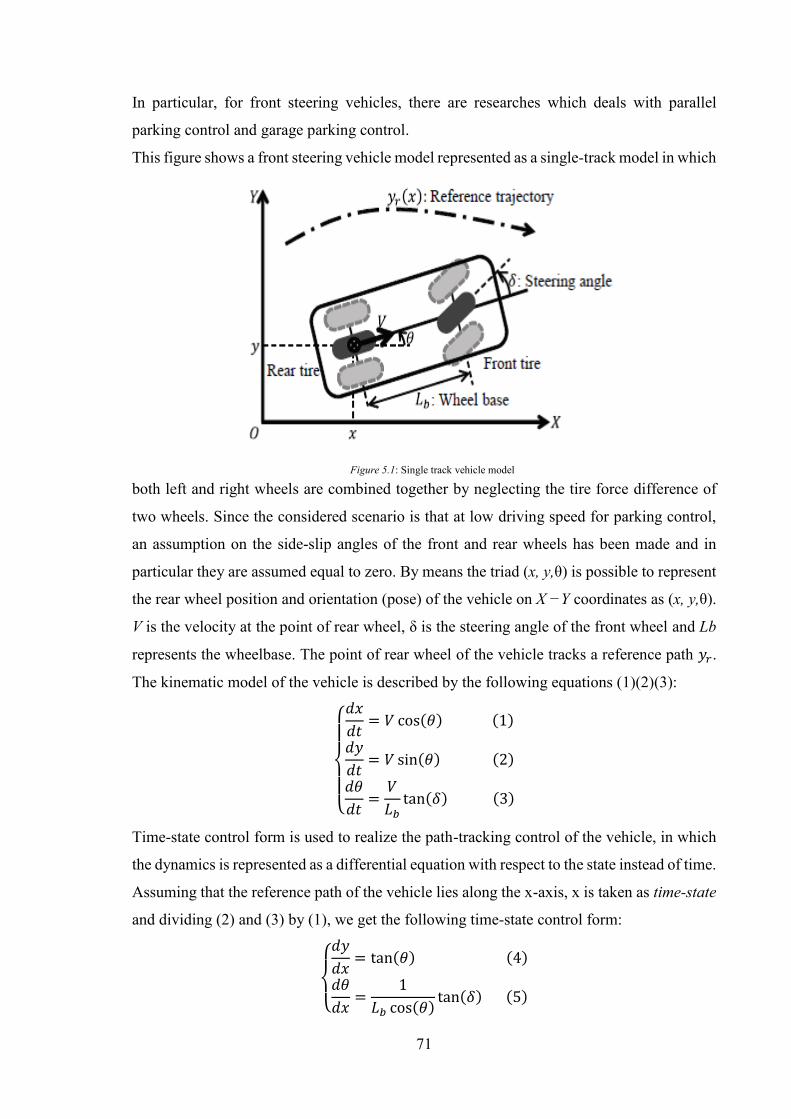
71

In particular, for front steering vehicles, there are researches which deals with parallel

parking control and garage parking control.

This figure shows a front steering vehicle model represented as a single-track model in which

both left and right wheels are combined together by neglecting the tire force difference of

two wheels. Since the considered scenario is that at low driving speed for parking control,

an assumption on the side-slip angles of the front and rear wheels has been made and in

particular they are assumed equal to zero. By means the triad (x, y,θ) is possible to represent

the rear wheel position and orientation (pose) of the vehicle on X −Y coordinates as (x, y,θ).

V is the velocity at the point of rear wheel, δ is the steering angle of the front wheel and Lb

represents the wheelbase. The point of rear wheel of the vehicle tracks a reference path 𝑦𝑟.

The kinematic model of the vehicle is described by the following equations (1)(2)(3):

{

𝑑𝑥

𝑑𝑡= 𝑉 cos(𝜃) (1)

𝑑𝑦

𝑑𝑡= 𝑉 sin(𝜃) (2)

𝑑𝜃

𝑑𝑡=𝑉

𝐿𝑏tan(𝛿) (3)

Time-state control form is used to realize the path-tracking control of the vehicle, in which

the dynamics is represented as a differential equation with respect to the state instead of time.

Assuming that the reference path of the vehicle lies along the x-axis, x is taken as time-state

and dividing (2) and (3) by (1), we get the following time-state control form:

{

𝑑𝑦

𝑑𝑥= tan(𝜃) (4)

𝑑𝜃

𝑑𝑥=

1

𝐿𝑏 cos(𝜃)tan(𝛿) (5)

Figure 5.1: Single track vehicle model

72

The next steps are the nonlinear state transformation (6) and input transformation (7) and

(8):

[

𝑧1𝑧2𝑧3] = [

𝑥𝑑𝑦/𝑑𝑥𝑦

] = [

𝑥tan(𝜃)𝑦

] (6)

𝜇1 = 𝑉 cos(𝜃) (7)

𝜇2 =1

𝐿𝑏cos3(𝜃) (8)

The transformation is defined in the range −𝜋/2 < 𝜃 < 𝜋/2. Starting from (6)(7)(8),

nonlinear state space equation (1)(2)(3) is transformed into the two following linear

subsystems: 𝑑𝑧1𝑑𝑡

= 𝜇1 (9)

𝑑

𝑑𝑧1[𝑧3𝑧2] = [

0 10 0

] [𝑧3𝑧2] + [

01] 𝜇2 (10)

where (9) equation is the differential equation of the time-state 𝑧1 with respect to the time t,

and (10) equation is the differential equation of other states 𝑧2 and 𝑧3 with respect to the

time-state 𝑧1. Using 𝜃 and 𝜇2 is possible to compute the actual steering 𝛿 by means the

following equation transformed from (8):

𝛿 = tan−1(𝐿𝑏cos3(𝜃)𝜇2)

Since the linearized time-state control form (10) is a double integrator system with respect

to the time-state x, it is straightforward to realize the path-tracking control if the desired path

𝑦𝑟 is described as a function of the time-state. In fact, if we apply

𝜇2 =𝑑2𝑦𝑟

𝑑𝑧12 − 𝑘2 (𝑧2 −

𝑑𝑦𝑟𝑑𝑧1

) − 𝑘1(𝑧3 − 𝑦𝑟)

with positive 𝑘1 and 𝑘2, then 𝑧3 → 𝑦𝑟 as 𝑧1 → ∞, which is achieved for positive 𝜇1 in (9).

For 𝑧1 → -∞, 𝑘1 > 0 and 𝑘2 < 0 is used to ensure stability. [12]

5.1 MATHEMATICAL ANALYSIS AND SIMULINK TSC DESIGN Starting from these two relations:

𝑑

𝑑𝑧1[𝑧3𝑧2] = [

0 10 0

] [𝑧3𝑧2] + [

01] 𝜇2

𝜇2 =𝑑2𝑦𝑟

𝑑𝑧12 − 𝑘2 (𝑧2 −

𝑑𝑦𝑟𝑑𝑧1

) − 𝑘1(𝑧3 − 𝑦𝑟)

it is possible to determinate the values of 𝑘1 and 𝑘2 to guarantee the stability of the system.

73

For this reason, the Routh criterion will be used after a substitution of 𝜇2 in the first relation:

𝑑

𝑑𝑧1[𝑧3𝑧2] = [

0 10 0

] [𝑧3𝑧2] + [

01] (𝑑2𝑦𝑟𝑑𝑧1

2 − 𝑘2 (𝑧2 −𝑑𝑦𝑟𝑑𝑧1

) − 𝑘1(𝑧3 − 𝑦𝑟)) =

= [𝑧20] + [

0𝑑2𝑦𝑟𝑑𝑧1

2 − 𝑘2𝑧2 + 𝑘2𝑑𝑦𝑟𝑑𝑧1

− 𝑘1𝑧3 + 𝑘1𝑦𝑟] = [

𝑧2𝑑2𝑦𝑟𝑑𝑧1

2 − 𝑘2𝑧2 + 𝑘2𝑑𝑦𝑟𝑑𝑧1

− 𝑘1𝑧3 + 𝑘1𝑦𝑟] =

= [𝑧2

−𝑘2𝑧2 − 𝑘1𝑧3]+[

0𝑑2𝑦𝑟

𝑑𝑧12 + 𝑘2

𝑑𝑦𝑟

𝑑𝑧1+ 𝑘1𝑦𝑟

] = [0 1−𝑘1 −𝑘2

] [𝑧3𝑧2] + [

01] (

𝑑2𝑦𝑟

𝑑𝑧12 + 𝑘2

𝑑𝑦𝑟

𝑑𝑧1+ 𝑘1𝑦𝑟)

The first step is to calculate the characteristic polynomial:

𝑃𝐾(𝐴) = |𝐴 − 𝜆𝐼| = |(

0 1−𝑘1 −𝑘2

) − (𝜆 00 𝜆

)| = |𝜆 1−𝑘1 −𝑘2 − 𝜆

| = 𝜆2 + 𝑘2𝜆 + 𝑘1

and so, one obtains:

∆ = 𝑘22 − 4𝑘1

Thus, the roots of the polynomial are:

𝜆1,2 =−𝑘2 ±√𝑘2

2 − 4𝑘1

2

which are the eigenvalues of the matrix.

By applying the Routh criterion to the characteristic polynomial, one arrives to find the

stability values:

𝜆2 + 𝑘2𝜆 + 𝑘1 = 0

|1 𝑘1𝑘2 0

→ |1 𝑘1𝑘2 0

|

−𝑘2= −𝑘2𝑘1−𝑘2

= 𝑘1

|1𝑘2𝑘1

𝑘10

from this table, it is needed to evaluate:

• sign permanence → roots with negative real part

• sign change → roots with positive real part

thus:

++|1k2k1

𝑘10

that is, 𝑘1 > 0 and 𝑘2 > 0.

These conditions allow to have a control system which guarantees the overall stability.

For this purpose, 𝑘1 = 1 and 𝑘2 = 0.1 are chosen.

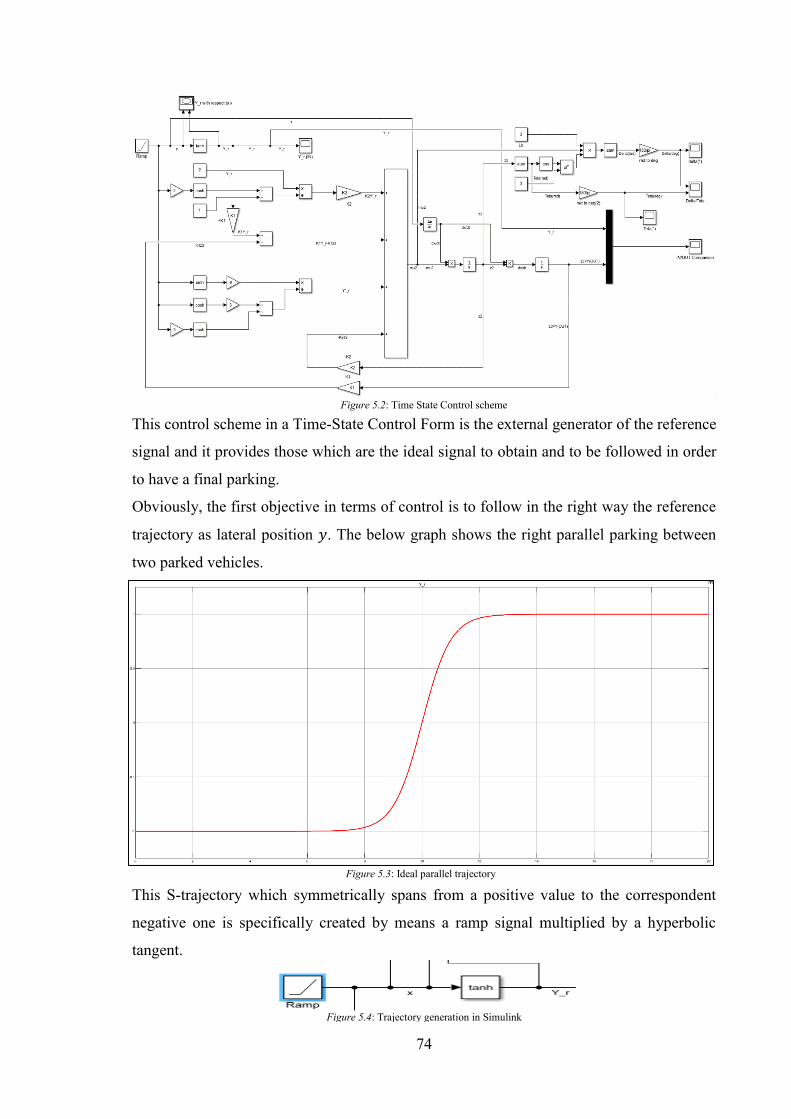
74

This control scheme in a Time-State Control Form is the external generator of the reference

signal and it provides those which are the ideal signal to obtain and to be followed in order

to have a final parking.

Obviously, the first objective in terms of control is to follow in the right way the reference

trajectory as lateral position 𝑦. The below graph shows the right parallel parking between

two parked vehicles.

This S-trajectory which symmetrically spans from a positive value to the correspondent

negative one is specifically created by means a ramp signal multiplied by a hyperbolic

tangent.

Figure 5.2: Time State Control scheme

Figure 5.3: Ideal parallel trajectory

Figure 5.4: Trajectory generation in Simulink

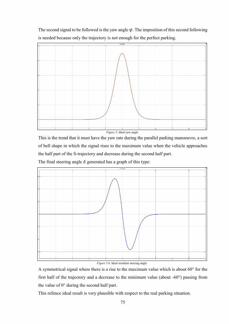
75

The second signal to be followed is the yaw angle 𝜓. The imposition of this second following

is needed because only the trajectory is not enough for the perfect parking.

This is the trend that it must have the yaw rate during the parallel parking manoeuvre, a sort

of bell shape in which the signal rises to the maximum value when the vehicle approaches

the half part of the S-trajectory and decrease during the second half part.

The final steering angle 𝛿 generated has a graph of this type:

A symmetrical signal where there is a rise to the maximum value which is about 60° for the

first half of the trajectory and a decrease to the minimum value (about -60°) passing from

the value of 0° during the second half part.

This refence ideal result is very plausible with respect to the real parking situation.

Figure 3: Ideal yaw angle

Figure 5.6: Ideal resultant steering angle

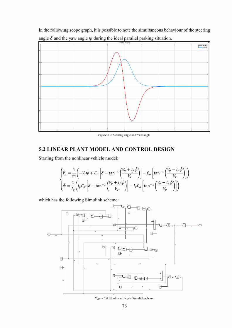
76

In the following scope graph, it is possible to note the simultaneous behaviour of the steering

angle 𝛿 and the yaw angle 𝜓 during the ideal parallel parking situation.

5.2 LINEAR PLANT MODEL AND CONTROL DESIGN Starting from the nonlinear vehicle model:

{

𝑉�� =

1

𝑚(−𝑉𝑥�� + 𝐶𝛼 [𝛿 − tan

−1 (𝑉𝑦 + 𝑙𝑓��

𝑉𝑥)] − 𝐶𝛼 [tan

−1 (𝑉𝑦 − 𝑙𝑟��

𝑉𝑥)])

�� =1

𝐼𝑧(𝑙𝑓𝐶𝛼 [𝛿 − tan

−1 (𝑉𝑦 + 𝑙𝑓��

𝑉𝑥)] − 𝑙𝑟𝐶𝛼 [tan

−1 (𝑉𝑦 − 𝑙𝑟��

𝑉𝑥)])

which has the following Simulink scheme:

Figure 5.7: Steering angle and Yaw angle

Figure 5.8: Nonlinear bicycle Simulink scheme

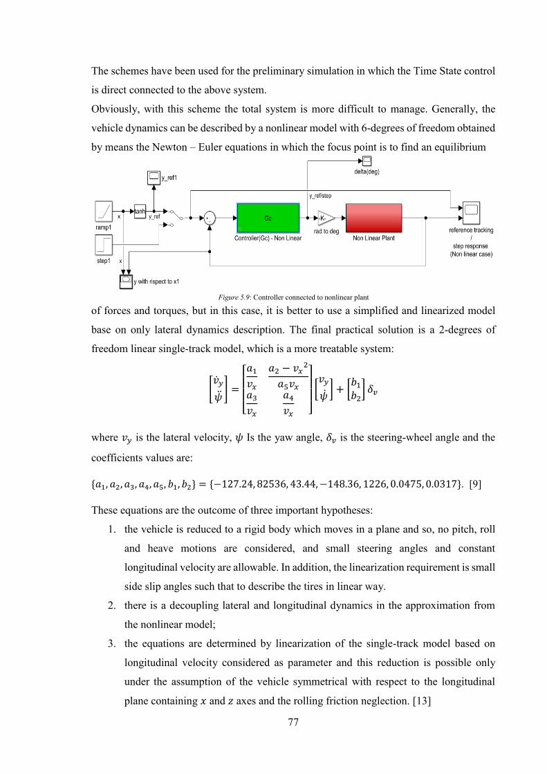
77

The schemes have been used for the preliminary simulation in which the Time State control

is direct connected to the above system.

Obviously, with this scheme the total system is more difficult to manage. Generally, the

vehicle dynamics can be described by a nonlinear model with 6-degrees of freedom obtained

by means the Newton – Euler equations in which the focus point is to find an equilibrium

of forces and torques, but in this case, it is better to use a simplified and linearized model

base on only lateral dynamics description. The final practical solution is a 2-degrees of

freedom linear single-track model, which is a more treatable system:

[��𝑦

��] =

[ 𝑎1𝑣𝑥

𝑎2 − 𝑣𝑥2

𝑎5𝑣𝑥𝑎3𝑣𝑥

𝑎4𝑣𝑥 ]

[𝑣𝑦

��] + [

𝑏1𝑏2] 𝛿𝑣

where 𝑣𝑦 is the lateral velocity, 𝜓 Is the yaw angle, 𝛿𝑣 is the steering-wheel angle and the

coefficients values are:

{𝑎1, 𝑎2, 𝑎3, 𝑎4, 𝑎5, 𝑏1, 𝑏2} = {−127.24, 82536, 43.44,−148.36, 1226, 0.0475, 0.0317}. [9]

These equations are the outcome of three important hypotheses:

1. the vehicle is reduced to a rigid body which moves in a plane and so, no pitch, roll

and heave motions are considered, and small steering angles and constant

longitudinal velocity are allowable. In addition, the linearization requirement is small

side slip angles such that to describe the tires in linear way.

2. there is a decoupling lateral and longitudinal dynamics in the approximation from

the nonlinear model;

3. the equations are determined by linearization of the single-track model based on

longitudinal velocity considered as parameter and this reduction is possible only

under the assumption of the vehicle symmetrical with respect to the longitudinal

plane containing 𝑥 and 𝑧 axes and the rolling friction neglection. [13]

Figure 5.9: Controller connected to nonlinear plant

78

The linear bicycle model represents the plant of the system:

which is modelized in Simulink by means the associated above equations:

The associated plant transfer functions need to be calculated:

𝐺𝑝 = [𝐺𝑝1 𝐺𝑝2]𝑇

In particular, the linear bicycle plant model can be written in state-space representation in

order to have a better vision of the single contribution of each element within the equations

and to simpler determinate the 𝐴, 𝐵, 𝐶, 𝐷 matrices for the next computations:

{�� = 𝐴𝑥 + 𝐵𝑢𝑤′ = 𝐶𝑥 + 𝐷𝑢

where:

• �� is the state vector:

�� = [��𝑦

��] = [

��

��]

• 𝑤′ and thus 𝑤 are the output vector and 𝑢 is the input (or control) vector:

𝑤′ = [��

��] and 𝑤 = [

𝑦𝜓] = [

𝐺𝑝1𝐺𝑝2

] 𝛿𝑣

• 𝐴 is the state (or system) matrix:

𝐴 =

[ 𝑎1𝑣𝑥

𝑎2 − 𝑣𝑥2

𝑎5𝑣𝑥𝑎3𝑣𝑥

𝑎4𝑣𝑥 ]

≅ [−45.81 21.4615.64 −53.41

]

Figure 5.10: Plant block

Figure 5.11: Linear bicycle Simulink scheme

79

• 𝐵 is the input matrix:

𝐵 = [𝑏1𝑏2] = [

0.04750.0317

]

• 𝐶 is the output matrix and it is imposed to be:

𝐶 = [1 00 1

]

• 𝐷 is the feedforward (or feedthrough) matrix and it is imposed to be:

𝐷 = [00]

From the output vector, one calculates the 𝐺𝑝 vector:

𝐺𝑝 = [𝐺𝑝1𝐺𝑝2

] =

[ 𝐺𝑝1′

𝑠𝐺𝑝2′

𝑠 ]

that is equal to calculate the terms of the 𝐻 matrix:

𝐻 = [𝐺𝑝1′

𝐺𝑝2′] = 𝐶(𝑠𝐼 − 𝐴)−1 ∙ 𝐵 + 𝐷 → [

𝐺𝑝1𝐺𝑝2

] =

[ 𝐺𝑝1′

𝑠𝐺𝑝2′

𝑠 ] →𝐺𝑝1 =

𝐻(1,1)

𝑠

𝐺𝑝2 =𝐻(2,1)

𝑠

imposing that the output vector:

𝑤′ = [1 00 1

] ∙ 𝑥 + [00] ∙ 𝑢

Thus, the computations are:

𝐻 = [1 00 1

] ∙

(

𝑠 [1 00 1

] −

[ 𝑎1𝑣𝑥

𝑎2 − 𝑣𝑥2

𝑎5𝑣𝑥𝑎3𝑣𝑥

𝑎4𝑣𝑥 ]

)

−1

∙ [𝑏1𝑏2] + [

00] =

= [1 00 1

] ∙ (𝑠 [1 00 1

] − [−45.81 21.4615.64 −53.41

])−1

∙ [0.04750.0317

] + [00]

well-defined in the MATLAB script:

and the final plant computed transfer functions are:

𝐺𝑝1 =0.0475

𝑠(𝑠 + 30.9), 𝐺𝑝2 =

0.0317

𝑠(𝑠 + 30.9)

the found transfer functions are those of a SITO system, where the single input is the steering

angle 𝛿, while the two outputs to be controlled are the lateral trajectory and the yaw angle.

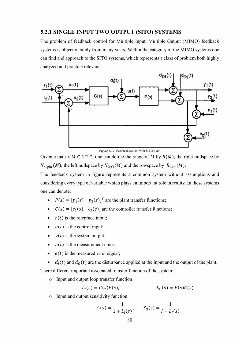
80

5.2.1 SINGLE INPUT TWO OUTPUT (SITO) SYSTEMS The problem of feedback control for Multiple Input, Multiple Output (MIMO) feedback

systems is object of study from many years. Within the category of the MIMO systems one

can find and approach to the SITO systems, which represents a class of problem both highly

analyzed and practice relevant.

Given a matrix 𝑀 ∈ 𝐶𝑚𝑥𝑛, one can define the range of 𝑀 by 𝑅(𝑀), the right nullspace by

𝑁𝑟𝑖𝑔ℎ𝑡(𝑀), the left nullspace by 𝑁𝑙𝑒𝑓𝑡(𝑀) and the rowspace by 𝑅𝑟𝑜𝑤(𝑀).

The feedback system in figure represents a common system without assumptions and

considering every type of variable which plays an important role in reality. In these systems

one can denote:

• 𝑃(𝑠) = [𝑝1(𝑠) 𝑝2(𝑠)]𝑇 are the plant transfer functions;

• 𝐶(𝑠) = [𝑐1(𝑠) 𝑐2(𝑠)] are the controller transfer functions;

• 𝑟(𝑡) is the reference input;

• 𝑢(𝑡) is the control input;

• 𝑦(𝑡) is the system output;

• 𝑛(𝑡) is the measurement noise;

• 𝑒(𝑡) is the measured error signal;

• 𝑑𝐼(𝑡) and 𝑑𝑂(𝑡) are the disturbance applied at the input and the output of the plant.

There different important associated transfer function of the system:

o Input and output loop transfer function

𝐿𝐼(𝑠) = 𝐶(𝑠)𝑃(𝑠), 𝐿𝑂(𝑠) = 𝑃(𝑠)𝐶(𝑠)

o Input and output sensitivity function:

𝑆𝐼(𝑠) =1

1 + 𝐿𝐼(𝑠), 𝑆𝑂(𝑠) =

1

𝐼 + 𝐿𝐼(𝑠)

Figure 5.12: Feedback system with SITO plant

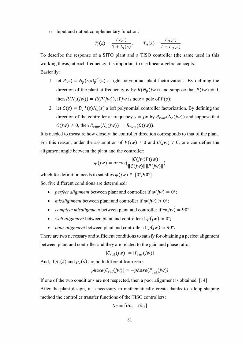
81

o Input and output complementary function:

𝑇𝐼(𝑠) =𝐿𝐼(𝑠)

1 + 𝐿𝐼(𝑠), 𝑇𝑂(𝑠) =

𝐿𝑂(𝑠)

𝐼 + 𝐿𝑂(𝑠)

To describe the response of a SITO plant and a TISO controller (the same used in this

working thesis) at each frequency it is important to use linear algebra concepts.

Basically:

1. let 𝑃(𝑠) = 𝑁𝑝(𝑠)𝐷𝑝−1(𝑠) a right polynomial plant factorization. By defining the

direction of the plant at frequency 𝑤 by 𝑅(𝑁𝑝(𝑗𝑤)) and suppose that 𝑃(𝑗𝑤) ≠ 0,

then 𝑅(𝑁𝑝(𝑗𝑤)) = 𝑅(𝑃(𝑗𝑤)), if 𝑗𝑤 is note a pole of 𝑃(𝑠);

2. let 𝐶(𝑠) = 𝐷𝑐−1(𝑠)𝑁𝑐(𝑠) a left polynomial controller factorization. By defining the

direction of the controller at frequency 𝑠 = 𝑗𝑤 by 𝑅𝑟𝑜𝑤(𝑁𝑐(𝑗𝑤)) and suppose that

𝐶(𝑗𝑤) ≠ 0, then 𝑅𝑟𝑜𝑤(𝑁𝑐(𝑗𝑤)) = 𝑅𝑟𝑜𝑤(𝐶(𝑗𝑤)).

It is needed to measure how closely the controller direction corresponds to that of the plant.

For this reason, under the assumption of 𝑃(𝑗𝑤) ≠ 0 and 𝐶(𝑗𝑤) ≠ 0, one can define the

alignment angle between the plant and the controller:

𝜑(𝑗𝑤) = 𝑎𝑟𝑐𝑜𝑠(|𝐶(𝑗𝑤)𝑃(𝑗𝑤)|

‖𝐶(𝑗𝑤)‖‖𝑃(𝑗𝑤)‖)

which for definition needs to satisfies 𝜑(𝑗𝑤) ∈ [0°, 90°].

So, five different conditions are determined:

• perfect alignment between plant and controller if 𝜑(𝑗𝑤) = 0°;

• misalignment between plant and controller if 𝜑(𝑗𝑤) > 0°;

• complete misalignment between plant and controller if 𝜑(𝑗𝑤) = 90°;

• well alignment between plant and controller if 𝜑(𝑗𝑤) ≈ 0°;

• poor alignment between plant and controller if 𝜑(𝑗𝑤) ≈ 90°.

There are two necessary and sufficient conditions to satisfy for obtaining a perfect alignment

between plant and controller and they are related to the gain and phase ratio:

|𝐶𝑟𝑎𝑡(𝑗𝑤)| = |𝑃𝑟𝑎𝑡(𝑗𝑤)|

And, if 𝑝1(𝑠) and 𝑝2(𝑠) are both different from zero:

𝑝ℎ𝑎𝑠𝑒(𝐶𝑟𝑎𝑡(𝑗𝑤)) = −𝑝ℎ𝑎𝑠𝑒(𝑃𝑟𝑎𝑡(𝑗𝑤))

If one of the two conditions are not respected, then a poor alignment is obtained. [14]

After the plant design, it is necessary to mathematically create thanks to a loop-shaping

method the controller transfer functions of the TISO controllers:

𝐺𝑐 = [𝐺𝑐1 𝐺𝑐2]

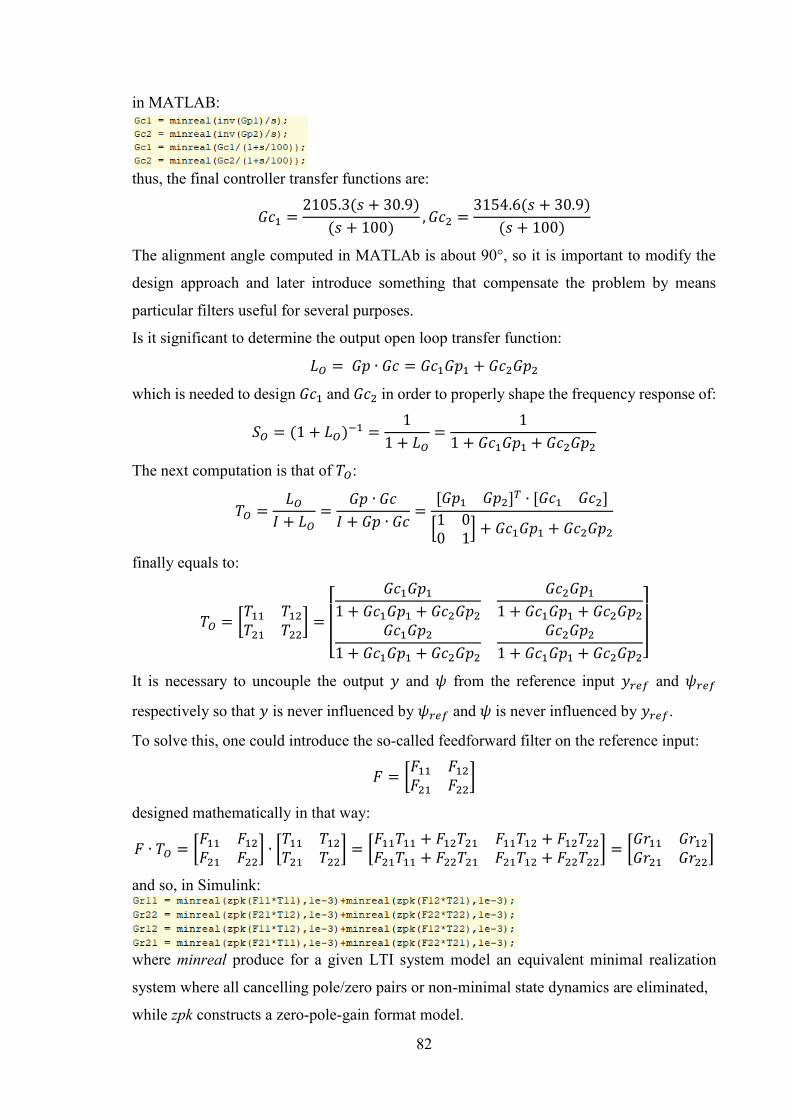
82

in MATLAB:

thus, the final controller transfer functions are:

𝐺𝑐1 =2105.3(𝑠 + 30.9)

(𝑠 + 100), 𝐺𝑐2 =

3154.6(𝑠 + 30.9)

(𝑠 + 100)

The alignment angle computed in MATLAb is about 90°, so it is important to modify the

design approach and later introduce something that compensate the problem by means

particular filters useful for several purposes.

Is it significant to determine the output open loop transfer function:

𝐿𝑂 = 𝐺𝑝 ∙ 𝐺𝑐 = 𝐺𝑐1𝐺𝑝1 + 𝐺𝑐2𝐺𝑝2

which is needed to design 𝐺𝑐1 and 𝐺𝑐2 in order to properly shape the frequency response of:

𝑆𝑂 = (1 + 𝐿𝑂)−1 =

1

1 + 𝐿𝑂=

1

1 + 𝐺𝑐1𝐺𝑝1 + 𝐺𝑐2𝐺𝑝2

The next computation is that of 𝑇𝑂:

𝑇𝑂 =𝐿𝑂

𝐼 + 𝐿𝑂=

𝐺𝑝 ∙ 𝐺𝑐

𝐼 + 𝐺𝑝 ∙ 𝐺𝑐=[𝐺𝑝1 𝐺𝑝2]

𝑇 ∙ [𝐺𝑐1 𝐺𝑐2]

[1 00 1

] + 𝐺𝑐1𝐺𝑝1 + 𝐺𝑐2𝐺𝑝2

finally equals to:

𝑇𝑂 = [𝑇11 𝑇12𝑇21 𝑇22

] =

[

𝐺𝑐1𝐺𝑝11 + 𝐺𝑐1𝐺𝑝1 + 𝐺𝑐2𝐺𝑝2

𝐺𝑐2𝐺𝑝11 + 𝐺𝑐1𝐺𝑝1 + 𝐺𝑐2𝐺𝑝2

𝐺𝑐1𝐺𝑝21 + 𝐺𝑐1𝐺𝑝1 + 𝐺𝑐2𝐺𝑝2

𝐺𝑐2𝐺𝑝21 + 𝐺𝑐1𝐺𝑝1 + 𝐺𝑐2𝐺𝑝2]

It is necessary to uncouple the output 𝑦 and 𝜓 from the reference input 𝑦𝑟𝑒𝑓 and 𝜓𝑟𝑒𝑓

respectively so that 𝑦 is never influenced by 𝜓𝑟𝑒𝑓 and 𝜓 is never influenced by 𝑦𝑟𝑒𝑓.

To solve this, one could introduce the so-called feedforward filter on the reference input:

𝐹 = [𝐹11 𝐹12𝐹21 𝐹22

]

designed mathematically in that way:

𝐹 ∙ 𝑇𝑂 = [𝐹11 𝐹12𝐹21 𝐹22

] ∙ [𝑇11 𝑇12𝑇21 𝑇22

] = [𝐹11𝑇11 + 𝐹12𝑇21 𝐹11𝑇12 + 𝐹12𝑇22𝐹21𝑇11 + 𝐹22𝑇21 𝐹21𝑇12 + 𝐹22𝑇22

] = [𝐺𝑟11 𝐺𝑟12𝐺𝑟21 𝐺𝑟22

]

and so, in Simulink:

where minreal produce for a given LTI system model an equivalent minimal realization

system where all cancelling pole/zero pairs or non-minimal state dynamics are eliminated,

while zpk constructs a zero-pole-gain format model.

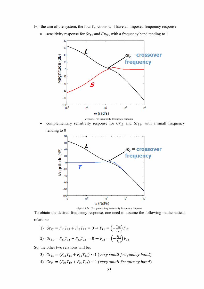
83

For the aim of the system, the four functions will have an imposed frequency response:

• sensitivity response for 𝐺𝑟11 and 𝐺𝑟22, with a frequency band tending to 1

• complementary sensitivity response for 𝐺𝑟12 and 𝐺𝑟21, with a small frequency

tending to 0

To obtain the desired frequency response, one need to assume the following mathematical

relations:

1) 𝐺𝑟12 = 𝐹11𝑇12 + 𝐹12𝑇22 = 0 → 𝐹11 = (−𝑇22

𝑇12)𝐹12

2) 𝐺𝑟21 = 𝐹21𝑇11 + 𝐹22𝑇21 = 0 → 𝐹21 = (−𝑇21

𝑇11)𝐹22

So, the other two relations will be:

3) 𝐺𝑟11 = (𝐹11𝑇11 + 𝐹12𝑇21) ~ 1 (𝑣𝑒𝑟𝑦 𝑠𝑚𝑎𝑙𝑙 𝑓𝑟𝑒𝑞𝑢𝑒𝑛𝑐𝑦 𝑏𝑎𝑛𝑑)

4) 𝐺𝑟11 = (𝐹21𝑇12 + 𝐹22𝑇22) ~ 1 (𝑣𝑒𝑟𝑦 𝑠𝑚𝑎𝑙𝑙 𝑓𝑟𝑒𝑞𝑢𝑒𝑛𝑐𝑦 𝑏𝑎𝑛𝑑)

Figure 5.14: Complementary sensitivity frequency response

Figure 5.13: Sensitivity frequency response

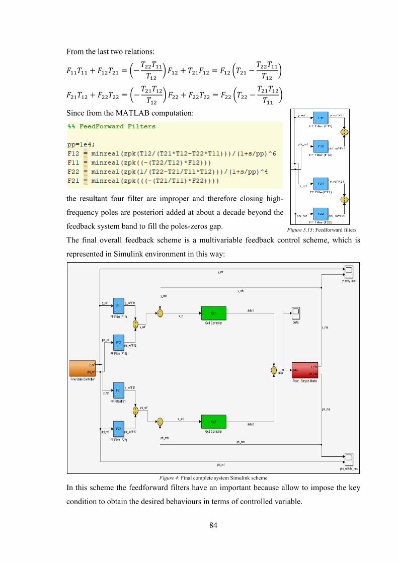
84

From the last two relations:

𝐹11𝑇11 + 𝐹12𝑇21 = (−𝑇22𝑇11𝑇12

)𝐹12 + 𝑇21𝐹12 = 𝐹12 (𝑇21 −𝑇22𝑇11𝑇12

)

𝐹21𝑇12 + 𝐹22𝑇22 = (−𝑇21𝑇12𝑇12

) 𝐹22 + 𝐹22𝑇22 = 𝐹22 (𝑇22 −𝑇21𝑇12𝑇11

)

Since from the MATLAB computation:

the resultant four filter are improper and therefore closing high-

frequency poles are posteriori added at about a decade beyond the

feedback system band to fill the poles-zeros gap.

The final overall feedback scheme is a multivariable feedback control scheme, which is

represented in Simulink environment in this way:

In this scheme the feedforward filters have an important because allow to impose the key

condition to obtain the desired behaviours in terms of controlled variable.

Figure 4: Final complete system Simulink scheme

Figure 5.15: Feedforward filters

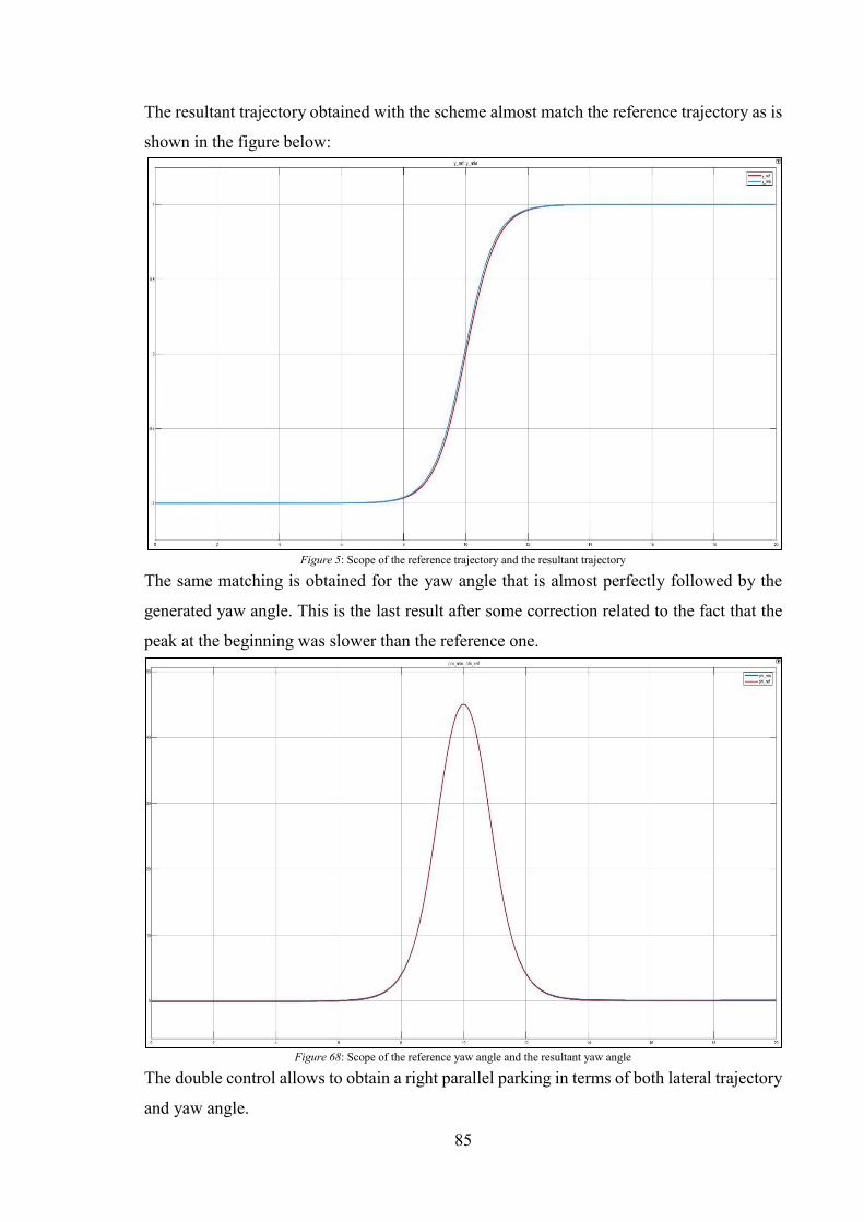
85

The resultant trajectory obtained with the scheme almost match the reference trajectory as is

shown in the figure below:

The same matching is obtained for the yaw angle that is almost perfectly followed by the

generated yaw angle. This is the last result after some correction related to the fact that the

peak at the beginning was slower than the reference one.

The double control allows to obtain a right parallel parking in terms of both lateral trajectory

and yaw angle.

Figure 5: Scope of the reference trajectory and the resultant trajectory

Figure 68: Scope of the reference yaw angle and the resultant yaw angle

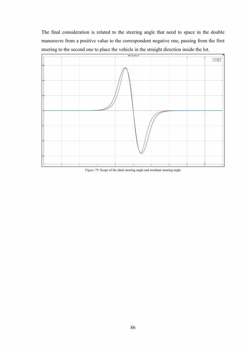
86

The final consideration is related to the steering angle that need to space in the double

manoeuvre from a positive value to the correspondent negative one, passing from the first

steering to the second one to place the vehicle in the straight direction inside the lot.

Figure 79: Scope of the ideal steering angle and resultant steering angle

87

CONCLUSIONS The obtained results show how the experienced approach as results of mathematical and

theoretical considerations can be used to face with a problem like a parking situation.

The analysis of the problem has highlighted the need to project a MIMO control system with

2-degrees of freedom composed by a feedback TISO controller and a feedforward filter used

to perform the decoupling of the reference signals effects on the outputs.

The approach tested on a SITO bicycle model system has given positive results even if

however, the performed tests are not very realistic because the model uncertainties have not

been taken into account.

Thus, the future developments are those of analysing the effect of the model uncertainty

presence and maybe considering no longer a linear model, but a nonlinear one.

88

LIST OF FIGURES 1.1 Remote-controlled vehicle……………………………………………………….......... 9

1.2 General Motors Prototype……………………………………………………………... 9

1.3 Tsubuka autonomous vehicle…………………………………………………………. 10

1.4 Dickmanns team vehicle……………………………………………………………… 10

1.5 Level of integration of companies that works in autonomy field…………………….. 11

1.6 Free driver from driving tasks………………………………………………………... 12

1.7 Autonomous vehicles levels………………………………………………………….. 13

1.8 Perception of the environment………………………………………………………... 14

1.9 Lane line marking detection………………………………………………………….. 16

1.10 LIDAR detection……………………………………………………………………. 17

1.11 LIDAR……………………………………………………………………………… 18

1.12 LIDAR Image……………………………………………………………………….. 19

1.13 DARPA CHALLENGE…………………………………………………………….. 21

1.14 Probabilistic Road Maps (PRM)…………………………………………………….. 24

1.15 Rapidly-exploring Random Trees (RRT)…………………………………………… 24

1.16 Decision making for obstacle avoidance……………………………………………. 25

2.1 Toyota Prius sensors (2003)………………………………………………………….. 31

2.2 Parking vision camera………………………………………………………………... 32

2.3 Volvo autonomous parking…………………………………………………………... 32

2.4 Direct trajectory planning…………………………………………………………….. 33

2.5 Planning scheme……………………………………………………………………… 34

2.6 Bicycle model - Forward motion…………………………………………………….. 35

2.7 Bicycle model - Backward motion…………………………………………………… 35

2.8 Possible trajectories…………………………………………………………………... 37

2.9 Specific trajectory……………………………………………………………………. 37

2.10 Steering angle sequence…………………………………………………………….. 37

2.11 From the initial to the finale state……………………………………………………. 38

2.12 Bicycle model representation……………………………………………………….. 39

2.13 Steering wheels and maximum rotation angle………………………………………. 40

2.14 Sensors information…………………………………………………………………. 40

2.15 Fuzzy controller……………………………………………………………………... 41

89

2.16 Inputs and outputs of controller……………………………………………………... 42

2.17 Controller conditions………………………………………………………………... 42

2.18 Four-wheeled car-like robot modelled as a bicycle…………………………………. 43

2.19 Gompertz curve movement of the vehicle centre……………………………………. 44

2.20 Gompertz curve function……………………………………………………………. 45

2.21 Parameter a evaluation……………………………………………………………… 45

2.22 Parameter b evaluation……………………………………………………………… 46

2.23 Parameter c evaluation………………………………………………………………. 46

2.24 Visualization of the optimal scheme result………………………………………….. 48

2.25 Evolution of trajectory based on b and c……………………………………………. 49

3.1 The functioning of a yaw control system……………………………………………... 51

3.2 The functioning of a yaw control system……………………………………………... 53

3.3 Ackerman turning geometry………………………………………………………….. 55

3.4 Differential steer from a trapezoidal tie-rod arrangement…………………………….. 56

3.5 Lateral vehicle dynamics……………………………………………………………... 57

3.6 Tire slip angle………………………………………………………………………… 58

4.1 Closed-loop system…………………………………………………………………... 64

5.1 Single track vehicle model……………………………………………………………. 72

5.2 Time State Control scheme…………………………………………………………… 75

5.3 Ideal parallel trajectory……………………………………………………………….. 75

5.4 Trajectory generation in Simulink……………………………………………………. 75

5.5 Ideal yaw angle……………………………………………………………………….. 76

5.6 Ideal resultant steering angle…………………………………………………………. 76

5.7 Steering angle and Yaw angle………………………………………………………… 77

5.8 Nonlinear bicycle Simulink scheme………………………………………………….. 77

5.9 Controller connected to nonlinear plant……………………………………………… 78

5.10 Plant block…………………………………………………………………………... 79

5.11 Linear bicycle Simulink scheme……………………………………………………. 79

5.12 Feedback system with SITO plant…………………………………………………... 81

5.13 Sensitivity frequency response……………………………………………………… 84

5.14 Complementary sensitivity frequency response…………………………………….. 84

90

5.15 Feedforward filters………………………………………………………………….. 85

5.16 Final complete system Simulink scheme………………………………………....... 85

5.17 Scope of the reference trajectory and the resultant trajectory……………………… 86

5.18 Scope of the reference yaw angle and the resultant yaw angle…………………….. 86

5.19 Scope of the ideal steering angle and resultant steering angle……………………... 87

91

BIBLIOGRAPHY [1] Markus Maurer, J. Christian Gerdes, Barbara Lenz, Hermann Winner, “Autonomous

Driving”, Springer, 2015

[2] Isabel Harne, “The 5 Autonomous Driving Levels Explained”,

https://www.iotforall.com/5-autonomous-driving-levels-explained/amp/, 2017

[3] Aakash Goel, “What Tech Will it Take to Put Self-Driving Cars on the Road?”,

https://www.engineering.com/DesignerEdge/DesignerEdgeArticles/ArticleID/13270/What-

Tech-Will-it-Take-to-Put-Self-Driving-Cars-on-the-Road.aspx, 2016

[4] Landmark Dividend, https://www.landmarkdividend.com/self-driving-car/

[5] Scott Drew Pendleton, Hans Andersen, Xinxin Du, Xiaotong Shen, Malika Meghjani,

You Hong Eng, Daniela Rus, Marcelo H. Ang Jr., “Perception, Planning, Control, and

Coordination for Autonomous Vehicles”, in machines, 2017

[6] Shubhankar Gautam, “A Brief History of Car Parking Technology”,

http://blog.getmyparking.com/2019/04/08/a-brief-history-of-car-parking-technology, 2019

[7] Wei Liu, Zhiheng Li, Li Li, Fei-Yue Wang, “Parking Like a Human: A Direct Trajectory

Planning Solution”, in IEEE Transactions on Intelligent Transportation Systems, 2017

[8] Denis M. Filatov, Elena V. Serykh, Michael M. Kopichev, Andrey V. Weinmeister,

“Autonomous Parking Control System of Four-Wheeled Vehicle”, in IEEE, 2016

92

[9] Aneesh N. Chand, Michihiro Kawanishi and Tatsuo Narikiyo, “Fast Parallel Parking for

Autonomous Vehicles using Gompertz Curve”, in IEEE, 2014

[10] Rajesh Rajamani, “Vehicle Dynamics and Control”, Springer, 2006

[11] Jean-Jacques E. Slotine, Weiping Li, “Applied Nonlinear Control”, Pearson plc., 1991

[12] Kentaro Oyama, Kenichiro Nonaka, “Model Predictive Parking Control for

Nonholonomic Vehicles using Time-State Control Form”, in European Control Conference,

2013

[13] V. Cerone, A.Chinu, D. Regruto, “Experimental Results in Vision-Based Lane Keeping

for Highway Vehicles”, in Proceedings of the American Control Conference, 2002

[14] Jim Freudenberg, Rick Middleton, “Properties of Single Input, Two Output Feedback

Systems”, in Proceedings of the American Control Conference, 1998