1

ConstructionofWeeklyStore‐LevelFoodBasketCosts 

DocumentationMay2016 

 

 

 

 

 

Project Title: Food Acquisition and Purchase Survey Geography Component (FoodAPS‐GC) 

Submitted by: 

Craig Gundersen, University of Illinois 

Kathy Baylis, University of Illinois 

Linlin Fan, University of Illinois 

Lisa House, University of Florida 

Paula Dutko, University of Florida 

   

  1

 

I. ObjectiveThe National Household Food Acquisition and Purchase Survey Geography Component (FoodAPS‐GC) 

investigates the relationship between local food environments and food spending by consumers in the 

United States. FoodAPS itself surveys 4,826 households in 50 primary sampling units (PSUs), each 

consisting of at least one county.   

FoodAPS‐GC has two main components under two cooperative agreements. The agreement with the 

University of Illinois focuses on describing retail food prices, carried out through a subcontract with the 

University of Florida, and using FoodAPS data to study the relationship between food environments and 

food spending patterns. The second agreement, with the Friedman School of Nutrition Science and 

Policy at Tufts University, aims to characterize the food environment within the 50 PSUs. 

This documentation describes retail food price data constructed by the University of Illinois and 

University of Florida. These data enable FoodAPS data users to compare prices faced by and options 

available to households across different store types and different geographical locations. To do so, 

weekly store‐level basket prices were constructed for stores within each of the 50 PSUs, as well as 

within counties adjacent to the PSUs. These basket prices are based on weekly Universal Product Code 

(UPC) level sales reported at the store and Regional Market Area (RMA) level. The process is modeled 

after Nielsen’s calculation of food basket prices based on the Thrifty Food Plan (TFP) for Feeding 

America’s Map the Meal Gap project (Gundersen et al. 2015).  

Table 1 lists the files created by this project and other relevant files. The file named basketprices 

contains calculations of the individual food category prices, median basket cost for a family of four, and 

the low‐cost of a food basket. A list of the PSUs and adjacent counties is provided in a file named 

PSU_adj_list.  

The TFP is used as a guide to categorize foods into groups and to assign recommended consumption 

quantities of these groups to households of different sizes and compositions. The file 

combined_tfpcategories assigns each food item (UPC) with a TFP category number. The data 

tfpdictionary is extracted from the USDA’s Center for Nutrition Policy and Promotion’s 2006 TFP report 

(CNPP, 2007) and shows the weekly recommended consumption in pounds for each TFP category for a 

family of four.  

Because the Information Resources, Inc. (IRI) data does not cover all stores that exist, the contractors 

made a list of counties that do not have any IRI stores in Counties_Missing_IRIStores. The detailed 

explanation of each variable in all datasets created by the contractors is provided in the 

Basket_Cost_Variable_List.xls. Included in table 1 are the explanations of these and other relevant 

datasets (iriweek_startdates, hhgeodata, BG2010_IRIstores_Proxmity20mi, Placeid_IRI_TempERSID) 

that are not created by this project but are useful to link basket costs with other FoodAPS datasets. 

Details on these linkage datasets are provided in section IV. The set of SAS programs and Stata do‐files 

  2

used to categorize the IRI items into TFP categories and to calculate the basket prices is included with 

these data files.   

II. DataA. FoodAPS

The National Household Food Acquisition and Purchase Survey (FoodAPS) was developed and funded by 

the U.S. Department of Agriculture’s Economic Research Service (ERS) and Food and Nutrition Service 

(FNS) to investigate patterns of food acquisition in households across the country. Over the period from 

April 2012 through January 2013, the survey collected food expenditure and acquisition data from 4,826 

households in 50 primary sampling units (PSUs) and 400 secondary sampling units (SSUs). FoodAPS PSUs 

consist of a single county or multiple adjacent counties, and SSUs represent Census block groups or 

blocks.  

Each household in FoodAPS kept a weekly food acquisition diary detailing items purchased, quantities 

purchased, prices paid, location of purchase, and means of payment, among other data. Household 

diaries were collected over different weeks, with each household reporting one week of data. In 

addition, detailed demographic data was collected for each household and its members. Details on how 

households may be linked with their PSU and stores within their PSU are laid out at the end of this 

document. Further information on how and what data was collected for the survey can be found in the 

FoodAPS User’s Guide. 

The main objective of this project was to estimate store‐level costs of a balanced diet that serve as 

proxies for the prices consumers pay in food retail stores in the FoodAPS PSUs and adjacent counties.  

To do so, the TFP food groupings and quantities of foods per person were used to characterize the 

amount of food across broad food groups that could be purchased for a balanced low‐cost diet. The TFP 

outlines how a household allocates its food budget to achieve a diet that meets the Dietary Guidelines 

for Americans at minimal cost. The TFP is constructed by USDA’s Center for Nutrition Policy and 

Promotion (CNPP, 2007) and specifies the quantities of groups of foods that people could purchase and 

consume at home to obtain a nutritious diet at a minimal cost for 15 different age‐gender groups. The 

cost of the TFP for a family of four serves as the basis for calculating Supplemental Nutrition Assistance 

Program (SNAP) benefit allotments. The TFP is not a specific shopping list but rather a guide to how 

much of each food group to purchase given the household’s size, age, and gender composition. The plan 

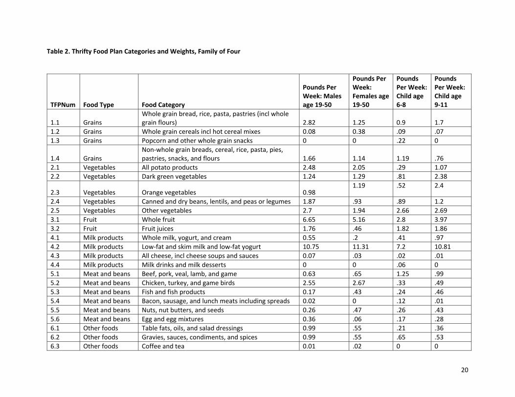
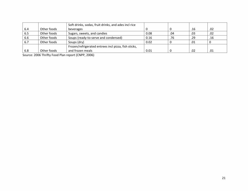
prescribes weekly quantities, in pounds, of food from 29 categories grouped under six broad food types:  

grains, vegetables, fruits, milk products, meat and beans, and other foods. Table 2 outlines these 29 

categories and quantities in detail and shows the tfpdictionary dataset. Quantities are based on the age 

and gender of the consumer, allowing TFP baskets to be constructed for an individual or aggregated 

over multiple individuals to create a household basket.  

Each TFP food group category is assigned a number to specify its broad food type and specific food 

category. For example, grains are type 1, and whole grain cereals is category 2 within food type 1; so 

foods classified as whole grain cereals are assigned the TFP number 1.2. 

  3

TFP weights for each food category are used for basket cost calculations. For each week of data reported 

by each store, the price per pound for each TFP category is calculated, then the category price is 

multiplied by recommended pounds for each individual of the family, and lastly, the cost of the TFP 

basket of goods for a family of four is totaled, consistent with the calculation for SNAP benefits. The 

basket cost is the sum of the cost of goods for a female age 19 to 50, a male age 19 to 50, a child age 6 

to 8 and a child age 9 to 11.   

Please note that these price data and cost calculations are based on each store’s sales of all food items 

in each category and include goods that would not necessarily be purchased by low‐income or SNAP 

households – for example, high‐quality cuts of meat or high‐end cheeses.  Also, note that the mix of 

items within a category, and hence the category price, may vary from store to store. Thus, these baskets 

are purposefully not called TFP food baskets. The TFP food groups and quantities are used as a model 

for categorizing and weighting grocery purchases to compose similar baskets across stores. These proxy 

basket costs do not represent the TFP or the lowest‐cost baskets and are not intended to reflect 

purchases made by typical SNAP recipients. 

Not all TFP food groups are available in all store‐weeks in the IRI database. Missing food groups are 

excluded from the store‐level basket costs, which reflects an incomplete basket of foods. A number of 

items sold in each store‐week‐food group is also counted. Further explanation of how this may affect 

the use of basket costs is provided in section III under the cost calculation discussion. 

B. IRIStoreScanner(InfoScan)DataTo construct the price per pound for each food category, food store scanner data was used; the data 

were provided by IRI, a private company that obtains, organizes, and sells retail store scanner data. The 

data provide weekly UPC‐level sales from store chains in the 50 FoodAPS PSUs, as well as in counties 

adjacent to these PSUs for each week of 2012. The 50 PSUs and their adjacent counties are referred to 

simply as the 50 PSUs throughout the rest of this document. The specific county list with county names 

(CountyName) and 5‐digit state+county FIPS code (county) for each PSU is in PSU_adj_list. The detailed 

explanation of each variable in PSU_adj_list is in Basket_Cost_Variable_List.xls.  

Most stores report UPC purchases and random‐weight purchases at the individual store level. Some 

store chains do not report prices at individual stores and instead permit sharing only aggregate sales at a 

Regional Market Area (RMA) level. RMAs may encompass geographically diverse areas and each store 

chain defines an RMA differently. For this reason, “chain” refers to a chain of stores and ”store” to a 

specific store location of that chain. Basket cost calculations are provided for both chains that report 

purchases at the store level and those that report at the RMA level.  

In addition, none of the RMA chains allow access to prices for private‐label (chain brand) items in UPC or 

random‐weight data. Target, Safeway and Kroger have private‐label data that are reported separately 

but they do not have item‐level purchase quantities. For this reason, private‐label items from Target, 

Safeway, Kroger and all 13 RMA chains in the food basket cost calculations are not included. 

Nevertheless, private‐label item purchases from over 28 non‐RMA chains with available data were 

included. Research has suggested that consumers allocate about 20 percent of their total spending on 

  4

consumer packaged goods to private‐label items (Planet Retail 2008). Because private‐label items are 

typically less expensive than national brand items, the exclusion of private‐label products may bias the 

basket cost estimates upward.  

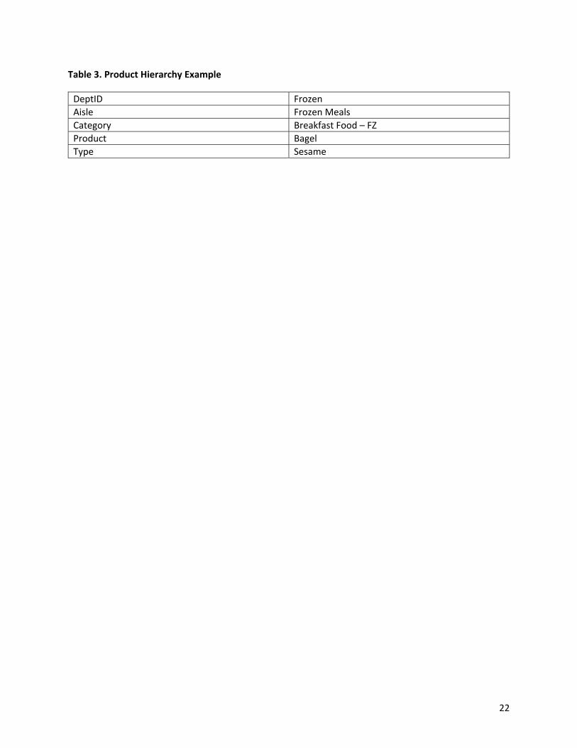
Sales data include total dollars paid and quantity purchased for each observation, where the unit of 

observation is the UPC or random‐weight item sold in a store‐week. All UPCs are classified, first by 

department (DeptID), then by Aisle, Category, and Product. These variables are listed in order of 

increasing detail. (See Table 3). 

Perishable or random‐weight items are classified by the same variables, but the type of information in 

these variables is less consistent across products. Random weight items do not have nutrition fact 

panels or front of package claims. Nevertheless, for some non‐random weight items, additional variables 

provide nutritional content details including front‐of‐package claims about fat, whole grains, sodium and 

other attributes, and back‐of‐package data from the nutrition panel.  

Two categories in the TFP – grains and dairy – separate sub‐categories based on nutrient content; thus 

two front‐of‐package claims (claim_whole_grain and claim_fat), as well as fat_content from the 

nutrition panel are used to categorize food items in these categories. The variable fat_content may be 

expressed in various ways, for example 7g fat, 93 percent lean, 4 percent milkfat, regular fat, or skim. 

The values for the two front‐of‐package claim variables are provided below. 

Claim_whole_grain values 

100 percent whole grain 

High whole grain 

Non h&w (health & wellness) category 

Not stated on package 

Other whole grain claim 

Source of whole grain 

Variety pack 

 

Claim_fat values 

Functional fat 

Less fat 

Low fat 

No fat 

Non h&w (health & wellness) category 

Not stated on package 

Other fat claim 

Variety pack

 

  5

III. MethodsA. Assigningproductstofoodcategories

The first step assigns each UPC‐coded item to a TFP category based primarily on the IRI classification 

variables, as described above.1 Both UPC items and perishables are classified primarily based on both 

the category and product variables.  

For four food categories, nutritional content is used to identify items: whole grain and non‐whole grain 

products, and whole milk and yogurt from reduced‐fat milk and yogurt. To separate whole‐grain 

products from refined‐grain products, both the type variable from the point‐of‐sale (pos) product 

dictionary and the claim_whole_grains variable from the master product dictionary file are used. 

Similarly, whole milk and full‐fat yogurt are distinguished from reduced‐fat versions, using the master 

product dictionary variables claim_fat and fat_content. Multiple variables are used to capture these 

differences due to inconsistent reporting in product data. For example, for many products, the type 

variable is blank or contains a flavor or variety description that does not include fat content or whole 

grain claims. Values for nutrition data, such as claim_fat are also missing for a large portion of products. 

Specifying multiple descriptive variables can capture differences in more products than using a single 

descriptive variable. In other words, few items are missing both claim_fat and fat_content.  When 

neither variable was available for a product and the product name did not indicate otherwise, it was 

assumed to be full fat content. 

In some stores and some weeks, products in a certain food category may not have been purchased or 

may simply have not been available. For example, in pharmacies or convenience stores, vegetables may 

not be offered; or such a narrow variety may be offered that they are rarely purchased. In many cases, 

the basket cost for a store‐week will then represent less than a “full” basket.  

The fact that some stores have more food groups than others, or more broadly speaking, some stores 

have more food items than others is often referred to as variety bias in the price index construction 

literature. While there are ways to tackle the variety bias when building a price index for a food basket, 

there are not any theoretically‐justified ways to solve this problem when calculating a proxy basket cost 

in dollar value. Therefore, basket costs were calculated regardless of whether all categories are available 

or purchased in a store‐week. Readers who are interested in price indices that address the variety bias 

may refer to section VI for more details. 

To highlight where basket costs may seem artificially low because they do not include all 29 categories 

of products, each of the basket cost files includes two variables to indicate whether and how many of 

the 29 total categories are sold in a store‐week. The variable tfpcats_availl is a count of the total 

number, out of 29, categories sold in a given store‐week. This may be used in conjunction with the 

binary variable fulltfp, which takes on a value of 1 if all 29 categories are sold, and a value of zero 

otherwise. 

                                                            1 The SAS program that categorizes each UPC into a TFP group is also provided. 

  6

B. Store‐levelcostsThe UPC purchase file was appended to the random‐weight purchase file and then the 5‐digit state + 

county FIPS code (county) and FoodAPS PSU number were merged to each store. For ease of 

computation, the purchase data were split into 50 files, one for each PSU in FoodAPS.2 The 50 files were 

later combined to create a single datasets for users called basketprices.  

Each item purchase was classified into a TFP category (classified numerically). In IRI, there are four units 

of measurement: ounces (“OZ”), dry ounces (“DRYOZ”), pounds (“LB”), and count (“COUNT”). “Count” is 

used as the unit of measurement for eggs and corn on the cob only. The weight of an egg uses the 

minimum required net weight for a “large” size egg specified by USDA, which is 2 oz or 0.125 lbs (USDA, 

2015). A “large”size egg is used because “large” is the most commonly used size of chicken egg and is 

the size commonly referred to for recipes (USDA, 2015). For corn on the cob, the weight for the Green 

Giant Extra Sweet Corn on the Cob with 8 mini corn ears (around 1 pound) is used, which is the most 

commonly purchased brand of corn on the cob in the IRI sales data. To calculate price per pound for 

each item, each unit of measurement in the IRI purchase data was converted to pounds as follows: 

1 OZ = 1/16 lbs_purchased 

1 DRYOZ=1/16 lbs_purchased 

1 COUNT = 0.125 lbs_purchased for eggs 

1 COUNT =1 lbs_purchased for corn 

Then the total pounds purchased for each item was calculated by multiplying the total volume with the 

number of pounds of each item. Food items of different sizes have different UPCs, such as a can of Coke 

and a pack of six Cokes. The volume recorded for a pack of Cokes indicates the number of packs 

purchased. Then the number of cans per pack is accounted for by using the larger weight of a pack of 

Coke. Typically, a pack of Coke weights 72 oz., while a can of Coke weights 12 oz. The number of pounds 

for a pack of Coke is calculated as 72/16=4.5 pounds. If the number of packs purchased in a store‐week 

(volume) is 10, then the total pounds purchased for packs of Coke in a store‐week is calculated as 

10*4.5=45 pounds. Price per pound is calculated by dividing the total expenditure on the item by the 

total pounds purchased. 

Some of the IRI store sales data have been cleaned by deleting food items that have prices less than the 

1st percentile or over the 99th percentile of the distribution of all store‐week food items prices. Unusually 

expensive food items are mostly spices, such as "saffron spice threads and flakes", "vanilla bean 

seasoning sticks", "bay leaf spice", or "chive spice", which are usually $1000‐$3000 per pound. The 

unusually cheap food items are carrots or water that could be less than $0.1 per pound. Because of low 

sales numbers for some food groups in some stores, these food items have prices equal to the median 

prices in their food group. Thus, taking the median for the respective category in a store‐week still does 

not solve the problem that unusually expensive or cheap items bias the prices for the TFP category. 

                                                            2 The SAS program containing calculations of basket prices for individual stores for each PSU cluster is also provided.   

  7

Therefore, those store‐week food items prices are deleted from the clean data before determining the 

median price.  The raw, uncleaned data were also used to calculate the median and low‐cost food 

baskets in basketprices_raw and are available to users.    

Three sets of costs/prices are calculated for these data for each PSU, that is, price per pound for each 

food category, median food basket cost for a family of four using the TFP quantities, and a “low‐cost” 

food basket cost for a family of four. The same sets of costs/prices are calculated for the raw data. 

Estimates of the different percentile category prices are not weighted by sales. 

First, a price for each TFP category by store‐week is calculated–for example, a price for whole grain 

cereals. The median price per pound by category for each week in each store was identified; the median 

was used instead of the mean price to avoid an unusually expensive or cheap item skewing the category 

and basket price. All items are simply ranked from the lowest to the highest price, regardless of how 

much of the item was purchased and then the median price was selected. The individual category price 

variables, category_price[xx], where [xx] represents the TFP category number assigned in table 2, 

multiplied by 10 to eliminate the decimal. Each category_price variable provides the median price per 

pound for an individual TFP category. A list of all variables and their definitions is provided in the 

Basket_Cost_Variable List.xls. 

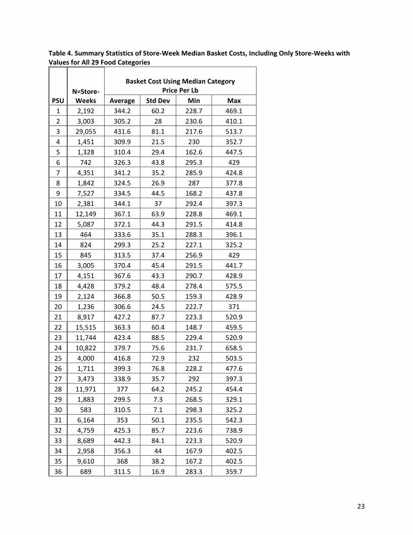
Next, a cost for the entire TFP basket for each store‐week was created, i.e. basket_price.  The median 

price per pound in each TFP category was multiplied by the pounds prescribed for purchase by the TFP 

for each individual in a family of four, and then these values were summed across individuals and 

categories in each store‐week. 

In addition to overall TFP costs, “low‐cost food basket costs” were calculated for each store‐week, 

low_basket_price. Different stores may offer higher quality goods in each category than other stores, 

skewing basket prices upward where customers are purchasing more expensive items from each 

category, like filet mignon rather than ground chuck, or organic fresh produce rather than non‐organic 

canned produce. To control for some of this variation, the per‐pound price at the 10th percentile was 

used in each of the 29 categories for each store‐week, and the total cost of the food category was 

constructed in the same way as when the median price was selected.  

Summary statistics of the median and low‐cost basket costs are provided in tables 4 and 5 for store‐

weeks that have all 29 TFP categories. These are by PSU. 

Admittedly, the proxy basket costs and low‐cost basket costs cannot guarantee that the food items are 

identical across stores or across time. The potential bias from comparing different products is called 

heterogeneity bias in the price index construction literature. There are ways to construct a price index, 

which is the relative price between a local store and a national average store that addresses the 

heterogeneity bias. Such methods were not used here because the aim is to build a proxy basket cost, 

not a price index per se. Interested readers may refer to section VI where the proxy basket costs are 

compared with various prices/price indices for more details. Another option is to identify the median 

cost good purchased in a category, or the median among low‐cost options, and then use that item for 

each store‐week. However, given that it is hard to find the identical or similar item(s) across all stores of 

  8

different types in the 50 geographically diverse PSUs, this approach to mitigate the heterogeneity bias 

issue was not used. 

C. RMA‐levelcostsBasket costs are also calculated for chains that report purchases only at the RMA level, using the same 

methodology of the store‐week level costs. Because store‐specific sales for each item cannot be 

observed in the RMA chains, all stores in the same RMA are assumed to have the same average 

calculated prices. A binary variable in the basketprices file, RMA, indicates whether the basket costs are 

from a chain reporting at RMA level (RMA=1) or at individual store level (RMA=0). From now on, RMA‐

level and store‐level combined are referred to as IRI stores.3 The variable geogkey, assigned by IRI, 

identifies the chain‐specific RMA in which each store is located and can be used to identify data from an 

RMA‐level store‐week where geogkey has a value. If the value of geogkey is missing, then it is a non‐

RMA store. 

IV. LinkingtoFoodAPSHouseholdandOtherFoodAPSDataIn using basket cost data, researchers will need to consider how to use the data to describe the 

household’s food price environment before matching the data to the FoodAPS household. This includes 

the geographic level at which to summarize the basket cost data and the time frame of reference (the 

store‐week(s) which best correspond to the time being studied, when the household reported 

purchases). Several files and variables within files can then be used to match the TFP basket cost data to 

the FoodAPS household.  

One option is to match store‐week data to the PSU in which the household resides. The file hhgeodata 

contains the psunum and the 5‐digit state + county FIPS code, county, with which the basketprices file 

can be merged to the household’s PSU.  A second option is to use the file 

BG2010_IRIstores_Proximity20mi, which contains a list of all the IRI stores within 20 miles of the 

population‐weighted centroid of the block groups in which FoodAPS households reside.  This file also 

contains a measure of the distance to each store from the block group centroid. This file can be matched 

to the basketprices file, using the Temp_ERS_ID variable and Placeid_IRI_TempERSID.  For those with 

a Third Party Agreement (TPA) with IRI, this Temp_ERS_ID variable can be used to match to other IRI 

store data files using Placeid_IRI_TempERSID.4 Matching BG2010_IRIstores_Proximity20mi to 

basketprices, allows users to develop summary measures of the food basket costs among all IRI stores 

within 20 miles of the block group centroid (or any other distance less than 20 miles). The  Temp_ERS_ID 

variable  and Placeid_IRI_TempERSID can also be used to link basketprices directly to the FoodAPS 

Places file (faps_places), which contains information about the stores visited by respondents or named 

as usual shopping venues.       

FoodAPS households reported their purchases and acquisitions for one week, sometime between April 

of 2012 and January of 2013.  Proxy basket costs by week for each store in the IRI data were created for 

                                                            3 The Stata do‐files for calculating basket prices using RMA data and appending this to store‐level basket prices are included with the other program files.   4 Further details about the IRI data are provided for users with a TPA with IRI.   

  9

January through December of 2012.  IRI reports data by week number, using its own week numbering 

system that begins at 1687 for the week starting on January 1, 2012. Weeks defined by IRI begin on 

Sunday and end on Saturday. The file iriweek_startdates provides the date of the Sunday on which each 

uniquely‐numbered IRI‐week begins in month/day/year format to more closely match the FoodAPS 

event dates. These IRI store‐week data can then be matched to the appropriate FoodAPS event date.  

Since IRI data for January 2013 are not available, users will have to use proxy measures of the basket 

costs from previous year’s data for households that were interviewed in January of 2013.  

V. DataLimitationsandCaveatsUsers of the calculated basket costs should bear in mind some important characteristics of the data used 

to create these costs.  

A. IRICoverageofStoresWhile IRI collects scanner data from a multitude of stores, only data from the subset of stores that have 

agreed to share their data with users (referred to as “cooperators”) may be made available to data 

purchasers. In some areas, then, the data may represent only a portion of the stores accessible to 

shoppers if the stores not represented by the IRI data differ systematically from those that are included, 

for example, in format or price range, this may skew basket cost calculations, as well as the picture of 

available food categories and store types.  

The number of IRI stores and the number of TDLinx stores were compared by retail channel and by PSU 

in PSU_Store_Count. TDLinx is a proprietary directory of stores produced by Nielsen and has a more 

comprehensive list of stores than IRI does. These numbers illustrate to what extent the IRI scanner data 

used to calculate prices represents the full set of stores from which consumers in each area may actually 

choose. 

Furthermore, some stores that do allow their price data to be shared with users only provide data at an 

aggregated level, namely RMA. For the RMA stores, average price for every store of the same RMA chain 

is used. As a result, the variation of store prices within the same RMA for the same chain may be lost.  

B. PurchasesVersusAvailableGoodsScanner data only provides records of goods that are actually purchased from a store and not an 

exhaustive picture of a store’s inventory. The IRI data for any given store‐week presents only those 

items that were purchased in that specific store during that week; so if certain goods are purchased less 

frequently in certain store types, the data may suggest narrower product availability than is true. For 

example, convenience stores may carry pre‐packaged deli meats, bacon, or similar products; but if 

customers rarely purchase these items from convenience stores, the scanner data will include no 

information on the availability and price of such goods at these outlet types.  

In these cases, calculated costs for a basket of goods represent an incomplete basket, and sometimes a 

very small portion of the entire set of product categories that comprise the basket. Costs calculated for 

such store‐weeks appear artificially low and imply a less diverse inventory than the store may carry in 

  10

reality. Researchers should keep this in mind when making inferences from the basket cost calculations. 

Therefore, the number of UPCs (count_upcxx) in the basketprices data is also provided. 

VI.ComparingOurFoodBasketCostswithOtherPrices/PriceIndicesThe basket costs created for the FoodAPS Geography project are meant to provide a measure of the cost 

of purchasing a nutritionally complete diet in a given store from a given week. These basket costs, which 

are based on the TFP food categories and quantities, were compared with four existing prices/price 

indices. Both Nielsen’s calculation for the Map the Meal Gap project and ERS’s Quarterly Food‐at‐Home 

Price Database measure food prices. These methods are compared with two commonly used price 

indices that include not only food but also other goods and services such as education, health care, and 

housing prices—one is the Cost of Living Index (COLI) by the Council for Community for Economic and 

Research that measures the ratio between city‐level average price and national average price for 

different cities. The second is the Consumer Price Index (CPI) which measures changes in price(s) over 

time. 

Each price/price index has advantages and shortcomings. In particular, two biases common in most 

price/price indices are heterogeneity bias and variety bias. Heterogeneity bias arises when product 

comparisons differ in each location or over time. For example, one might use the average price of bread 

per pound to compare the prices of bread across stores, but the bread compared in store A includes a 

high‐value ‘artisanal whole grain’ option, whereas the bread in store B does not. Thus a higher price of 

bread in store A may indicate bread in store A has higher quality rather than having higher price for the 

exactly same bread. The indices created by Broda and Weinstein (2010), Handbury and Weinstein (2014) 

and Hottman (2014) address this shortcoming.  

Variety bias occurs when some stores offer food options that other stores don’t have. To achieve the 

same level of utility, households need to pay more for other food options to substitute the missing food 

item. Both product heterogeneity bias and variety bias can be addressed by assuming constant 

elasticities of substitution preferences and using national expenditure shares data. These sets of price 

indices are called variety‐adjusted price indices (Feenstra 1994; Broda and Weinstein 2010: Handbury 

and Weinstein 2014; Hottman 2014).  

A.SummaryofComparisonsFoodAPS Weekly Store‐Level Food Basket Costs 

Uses IRI store sales data (both UPC and random‐weight purchases) 

Calculates a weekly TFP basket price for each store. For RMA stores, a weekly TFP basket price is calculated for each chain, and prices for each store in the RMA are assumed to be the same. 

For each TFP category the median price is chosen and weighted by the TFP category weights for a family of four (male age 19 to 50, female age 19 to 50, child age 6 to 8, child age 9 to 11).  

For a second index, the 10th percentile of price for each category is used, to calculate the price of a “low‐cost food basket”.  

  11

Pros: Captures both time and store variation in food basket cost; uses median TFP category prices to remove the effects of outliers on prices (the very expensive or cheap goods); uses the 10th percentile price of each category to capture low‐cost basket of food. 

Cons: Cannot guarantee that the goods compared over time and over stores are identical (product heterogeneity bias). Some goods are available in some stores at certain times but are not available in other stores and/or at other times (variety bias). Given that goods are not perfect substitutes, unavailability of a good will cause the minimum cost of achieving the given level of utility to rise. Missing TFP category prices occur when stores do not have any purchase records in the TFP category. We do not impute for any of those missing TFP category prices, but include a variable indicating the number of available TFP categories in a store‐week.  

Nielsen’s calculation of Thrifty Food Plan (TFP) basket prices for Feeding America’s Map the 

Meal Gap project 

Uses 12 weeks of Nielsen store sales data and four weeks of Nielsen Homescan purchase data if store sales data are not available (both random weight and UPC). 

Calculates an annual TFP basket price for each county. 

For each TFP category in a county, total spending for the TFP category is divided by total quantity sold for the category to obtain the TFP category price. Then TFP weights for males age 19 to 50 are used to capture the prices for a basket. 

For counties where no sales are recorded for a TFP category or small sales in categories have distorted the overall market basket prices, Nielsen imputes the prices for the TFP category with an average of the surrounding counties (Gundersen et al. 2010).  

Pros: Uses expenditure‐weighted prices to calculate TFP category prices (total spending divided by total quantity) to better reflect consumer behavior. 

Cons: Product heterogeneity bias and variety bias. TFP cost for a county may be too broad for food desert definitions.  

Quarterly Food‐at‐Home Price Database  

Uses 2004‐2010 Nielsen Homescan Data (UPC purchases only).  

Calculates a quarterly price for each of the 54 food groups in each metropolitan city from 2004 to 2010. 

For each food group purchased by a sample household in a quarter, the average price is calculated by dividing the sum of prices by the number of times the goods are purchased. For example, if a household purchases bread four weeks in a quarter, then the average price is the sum of 4 prices divided by 4 weeks. Then each household purchase price for a food group is weighted by the household sampling weights to derive a city‐level price for the food group (Todd et al. 2010). Any price per 100 grams that is greater than 4 standard deviations above the market quarter mean is considered an outlier and dropped from the dataset (Todd et al. 2010).  

Pros: Captures the city and quarterly variation of food group prices. 

Cons: Product heterogeneity bias and variety bias; Does not include random weight products including some meat, fresh fruits, and vegetables compared with packaged fruit, vegetables and meat. This may bias the average cost of the TFP basket. The definition of a market is broad and might not be relevant to a particular household. 

  12

 

Variety‐adjusted Price Indices (Feenstra 1994; Broda and Weinstein 2010; Handbury and 

Weinstein 2014; Hottman 2014) 

Uses Nielsen Homescan Data (Broda and Weinstein 2010; Handbury and Weinstein 2014) or Nielsen Kilts Store data (Hottman 2014). The price index takes price and available variety into account. Feenstra (1994) introduces the variety‐adjusted price index as the minimum cost to achieve one unit of utility. By imposing nationwide homogeneous nested Constant Elasticity of Substitution (CES) preferences, the minimum cost or the variety‐adjusted price index has an analytical form and is a function of market shares for each good, prices for each good, and elasticities of substitution between goods. Market shares and prices are observed, and elasticities of substitution can be estimated from the data. To compare price indices of goods of the same quality across time, Broda and Weinstein (2010), Handbury and Weinstein (2014), and Hottman (2014) implicitly assume quality equals utility. Namely, one unit of quality for a UPC is equal to the amount of utility obtained from one unit of consumption of the UPC. Then the quality‐adjusted or variety‐adjusted price index for a given period can be calculated as the minimum cost in that period to achieve the same amount of utility (quality) across time or across space. Therefore prices of each UPC are weighted by elasticities of substitution between and within food groups along with national market shares of each UPC. 

Broda and Weinstein (2010) calculate an annual price index for goods that includes not only groceries but also health, beauty and household supply products from 1999 to 2003 for the United States. Handbury and Weinstein (2014) calculate a city‐level price index for food specifically in 2005. Hottman (2014) constructs a quarterly variety‐adjusted store price index based on prices of not only food but also health, beauty, and household supply product groups. Then he uses quarterly store price indices in the county to construct the quarterly county‐level variety‐adjusted price index.  

Pros: Adjusts for product heterogeneity and variety bias. 

Cons: Elasticities of substitution are not easy to estimate. Results depend on the CES assumption. 

 

Two Price Indices that are not based on the IRI or Nielsen Data  

Cost of Living Index (COLI) by Council for Community and Economic Research 

Data are collected by field agents for six major categories: grocery items, housing, utilities, transportation, health care, and miscellaneous goods and services in different cities across the United States. To calculate a price for each category, a non‐random sample of items is chosen from that category. For example, when they use a pound of fuji apples to represent fruits, they assume that if an area’s price for fuji apples are 20 percent above the nationwide average, its prices for fruits as a whole also are about 20 percent above the nationwide average. Weights for each category are based on expenditure shares of the Consumer Expenditure Survey 2004. 

Calculates the ratio of the average price collected for each item in each city and quarter relative to its national average in that quarter (a price index not price per se).    

Pros: Captures variation in prices across city and time; compares similar goods across cities. 

Cons: Does not compare identical goods (heterogeneity bias), variety bias. The good chosen may not represent the whole category. 

  13

 

Consumer Price Index (CPI) 

Data collected by field agents for the Bureau of Labor Statistics (BLS). 

A national‐level price index for each month. The CPI is a measure of price change not price level per se. The reference base is 1982‐84 and BLS sets the average CPI for the 36‐month period covering 1982‐1984 to be 100. Then BLS measures price changes relative to the price in 1982‐1984.The CPI includes both food and other goods and services such as housing, education and medical care. Each category price is weighted by expenditure shares indicated by the 2011‐2012 Consumer Expenditure Survey.  

BLS has local CPI data at the metropolitan level (e.g. Chicago‐Gary‐Kenosha, IL‐IN‐WI), but the local CPI data are not comparable across space because CPI only measure the price change not price per se. A higher CPI indicates a higher price increase rather than higher price.  

Pros: Comprehensive inclusion of all consumer goods and services. 

Cons: Cannot be used to compare prices across space; cannot ensure products compared across time are identical (quality may be different, heterogeneity bias), variety bias. 

   

  14

B.DetailedExplanationofEachPrice(Index)Nielsen’s calculation of Thrifty Food Plan (TFP) basket prices for Feeding America’s Map the Meal Gap 

project. 

To derive a dollar value for a typical weekly basket of food by county for the Map the Meal Gap project, Nielsen uses the Nielsen Scantrack store sales data that have a similar structure as the IRI store sales data. The locations of stores are extracted from the TDLinx database. For stores that do not exist in the sales data, they use purchase records from the Nielsen Homescan database to impute food prices. Each observation in the Nielsen Homescan database represents the purchase of an individual UPC in a particular store by a particular consumer on a particular day. 

 Nielsen chooses the mix of food based on the USDA Thrifty Food Plan for males 19‐50 years old. For each year's value, they use 4 weeks of data from the store sales database and 12 weeks of data from the Homescan database.  From that data, they calculate a value of price per pound for each category and county (total spending for the TFP category divided by total quantity sold for the category). They then weight the category values by the Thrifty Food Plan weighting to arrive at a TFP basket value for each county. 

 Nielsen’s calculations of TFP basket prices differ from the food basket costs method in that they use total spending for the TFP category divided by total quantity sold for the category at the category price.5 In the food basket costs method, the price for each UPC in the category is calculated using the total spending on the UPC divided by the total quantity sold on the UPC. Then the median UPC price or the lowest 10th percentile price of the category is chosen to construct the category price. Therefore, Nielsen’s method puts more weight on the prices of the UPCs that have larger expenditures within a category to derive the category price while the food basket costs method puts all weight on the UPC with the median price. Moreover, Nielsen calculates an annual TFP cost for a county while the food basket costs method calculates weekly TFP cost at store levels. In addition, Nielsen uses the TFP for one person while the food basket costs method uses the TFP for a family of four. One other difference is that Nielsen estimates a basket cost for all counties in the U.S., whereas the food basket costs method calculates weekly store price indices only for the PSUs in FoodAPS.    Note that other research has used market share weighted prices for a category to calculate a weighted average price of a category. 

Quarterly Food‐at‐Home Price Database 

The Quarterly Food‐at‐Home Price Database (QFAHPD‐2) was developed by ERS (Jessica E. Todd, Lisa 

Mancino, Ephraim Leibtag, and Christina Tripodo) in 2010 and updated in 2012 to provide market‐level 

(Nielsen‐defined metropolitan areas) food prices. The database, constructed from 2004‐2010 Nielsen 

Homescan data, includes quarterly observations on the mean price of 54 food categories for 35 market 

groups covering the contiguous United States.  

                                                            5 This approach is different from the average UPC price for the TFP category in that to calculate the average UPC price, first each UPC price is calculated by dividing the total spending on the UPC by the total quantity spent on the UPC. Then the average UPC price for each TFP category is the mean of all UPC prices in the category. 

  15

 

After 2007, the Nielsen Homescan data reports less detailed information on random‐weight purchases. Therefore, ERS excluded the random‐weight purchases for the second version of QFAHPD and based all price calculations on Point of Sale (POS) purchases only. They aggregated the purchase data by first constructing for each household “i” the average price of food group “k” in quarter “q” (pi,k,q) (Todd et al. 2010). Each purchase occasion is weighted equally (by household average price) regardless of the expenditure on the item in each occasion. Essentially, the mean food group price is weighted by the number of times purchased. For example, if a household purchases apples in four weeks of one quarter, the household mean quarterly price for apples is the simple mean of the 4 prices. Then households are weighted by sampling weights in the market.    Feenstra (1994), Broda and Weinstein (2010), Handbury and Weinstein (2014), Hottman (2014) 

Variety‐Adjusted Price Indices 

Feenstra (1994) first introduces and calculates the gains from variety in the international trade literature 

because goods are not perfect substitutes for other goods. The variety‐adjusted price index is the 

minimum cost to achieve one unit of utility. By imposing nationwide homogeneous nested Constant 

Elasticity of Substitution preferences, the minimum cost or the variety‐adjusted price index has an 

analytical form and is a function of market shares for each good, prices for each good, and elasticities of 

substitution between goods. Market shares and prices are observed and elasticities of substitution can 

be estimated from the data. To compare price indices of goods of the same quality across time, they 

implicitly assume quality equals utility. Namely, the quality obtained from one unit of consumption of a 

UPC is equal to the amount of utility obtained from one unit of consumption of the UPC. Then the 

quality‐adjusted or variety‐adjusted price index for a given period can be calculated as the minimum 

cost in that period to achieve the same amount of utility (quality) across time. 

Broda and Weinstein (2010) use Feenstra’s (1994) insight to construct a quality‐adjusted or variety‐

adjusted price index for the whole US for each year (1994 and 1999‐2003). They use the Nielsen 

Homescan data that cover not only grocery items, but also health, beauty and other household supply 

sectors. Broda and Weinstein (2010) find that the quality‐adjusted price index that takes product 

turnover into account is 0.8 percentage points per year lower than a “fixed goods” price index like the 

CPI. This difference occurs because CPI does not adjust for the fact that the newly created products are 

of higher quality than the replaced old products that disappear in the markets. After adjusting for the 

quality improvement, the price index is lower than CPI. 

 Handbury and Weinstein (2014) apply the inter‐temporal price index from Broda and Weinstein 

(2010) into a spatial context and focus on food specifically. They calculate a variety‐adjusted price 

index for each of the 49 cities in the US that are covered in the 2005 Nielsen Homescan data. They 

identify two important sources of bias. Heterogeneity bias arises from comparing different goods in 

different locations, and variety bias arises from not correcting for the fact that some goods are 

unavailable in some locations. They eliminate heterogeneity bias by using UPC level prices rather than 

unit prices of broad food categories and controlling for store fixed effects. Eliminating the heterogeneity 

  16

bias causes 97 percent of the variance in the price level of food products across cities to disappear 

relative to a conventional index. They remove the variety bias by using the same method as Feenstra 

(1994) and Broda and Weinstein (2010), namely calculating the minimum cost in each city to achieve 

one unit of utility. Eliminating both heterogeneity and variety biases reverses the common finding that 

prices tend to be higher in larger cities. Instead, they find that price level for food falls with city 

population. 

When cleaning the Nielsen Homescan data, Handbury and Weinstein (2014) note that in cases where 

panelists shop at stores without scanner technology, panelists report the price paid manually. Since 

errors can be made in this reporting process, Handbury and Weinstein (2014) discard any purchase 

records for which the price paid was greater than twice or less than half the median price paid for the 

same UPC, approximately 250,000 out of 16 million observations (Footnote 8). Each observation 

represents the purchase of an individual UPC in a particular store by a particular consumer on a 

particular day. Handbury and Weinstein (2014) do not include random‐weight items because the quality 

of random weight items, such as fruit, vegetables, and deli meats, varies over time as the produce loses 

its freshness. They cannot control for this unobserved heterogeneity in quality (Handbury and Weinstein 

(2014) Footnote 10). 

Hottman (2014) use the same method as Handbury and Weinstein (2014) to calculate a quarterly 

variety‐adjusted store price index in each of the sample urban counties from 2006 to 2010. Then he 

uses quarterly store price indices in the county to construct the quarterly county‐level variety‐adjusted 

price index. He uses Nielsen Kilts retailer data (data collection point is store), which is also store sales 

data like the IRI store‐scan data, as opposed to Nielsen Homescan data (data collection point is 

household). He finds that retail store variety significantly affects the cost of living in the county.  

 

Consumer Price Index (CPI) 

 The Consumer Price Index (CPI) is a measure of the average change over time in the prices paid by 

urban consumers for a market basket of consumer goods and services. The data for the CPI come from 

the Bureau of Labor Statistics (BLS) field agent surveys of stores from a sample of products. It is a 

measure of price change not a change in price level per se. Most of the specific CPI have a 1982‐84 

reference base. That is, BLS sets the average price index level for the 36‐month period covering the 

years 1982, 1983, and 1984‐equal to 100. BLS then measures changes in prices in relation to that base. 

An index of 110, for example, means there has been a 10‐percent increase in price since the reference 

period; similarly, an index of 90 means a 10‐percent decrease.  

CPI includes both food and other goods and services. The weights are defined by the household 

expenditure shares on each of the goods and services in the 2011‐2012 Consumer Expenditure Survey. 

Major groups and examples of categories included in the CPI are food and beverages, housing, apparel, 

transportation, medical care, recreation (e.g. toys, sports equipment, admissions), and education and 

communication. The CPI also includes sales tax and government‐charged user fees. There are about 200 

  17

item categories in the CPI in total. Within each item category, several hundred specific items are chosen 

to represent several thousands of varieties of that item category. 

Limitations in measurement (product heterogeneity) Products chosen in each time period may differ due to the fact that the original sample item is replaced by the manufacturer with an upgraded one. For example, if the three mega‐pixel camera is replaced with four mega pixel camera in a given month in the sample store, then the new four mega‐pixel camera is included in the CPI. CPI assumes the price changes are for the identical camera, not due to quality changes.  Limitation in Applications The local indices (metropolitan level, e.g. Chicago‐Gary‐Kenosha, IL‐IN‐WI) are not comparable across 

space. A higher CPI in city A compared to B only means the price increased by a larger percentage in city 

A than B. 

 

ACCRA Cost of Living Index (COLI) 

 Given the limitation of the CPI in gauging the price differences across areas, the Council for Community 

and Economic Research (formerly the ACCRA) calculates a Cost of Living Index to compare price levels 

across cities. ACCRA collects prices for six major categories: grocery items, housing, utilities, 

transportation, health care, and miscellaneous goods and services in different cities across the United 

States. To calculate a price for each category, a non‐random sample of items is chosen from that 

category. For example, when they use a pound of fuji apples to represent fruits, they assume that if an 

area’s price for fuji apples are 20 percent above the nationwide average, its prices for fruits as a whole 

also are about 20 percent above the nationwide average. Weights for each category are based on 

expenditure shares of the Consumer Expenditure Survey 2004. ACCRA takes the ratio of the average 

price collected for each item in each city and quarter relative to its national average in that quarter. 

The ACCRA Cost of Living Index (COLI) is a weighted average of these ratios, where item weights are 

based on expenditure shares from the U.S. Bureau of Labor Statistics 2004 Consumer Expenditure 

Survey. See http://www.coli.org/Method.asp for more details.  

Limitations 

There are a host of problems arising from comparing prices of similar (as opposed to identical) products. 

Variety bias exists too. 

   

  18

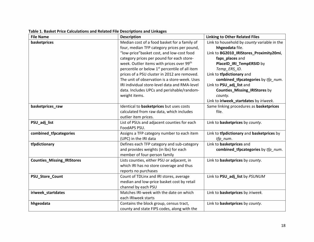
Table 1. Basket Price Calculations and Related File Descriptions and Linkages 

File Name  Description  Linking to Other Related Files 

basketprices  Median cost of a food basket for a family of four, median TFP category prices per pound, “low‐price”basket cost, and low‐cost food category prices per pound for each store‐week. Outlier items with prices over 99th percentile or below 1st percentile of all item prices of a PSU cluster in 2012 are removed. The unit of observation is a store‐week. Uses IRI individual store‐level data and RMA‐level data. Includes UPCs and perishable/random‐weight items. 

Link to household by county variable in the hhgeodata file.   

Link to BG2010_IRIStores_Proximity20mi, faps_places and PlaceID_IRI_TempERSID by Temp_ERS_ID.  

Link to tfpdictionary and combined_tfpcategories by tfp_num. 

Link to PSU_adj_list and Counties_Missing_IRIStores by county.  

Link to iriweek_startdates by iriweek. 

basketprices_raw  Identical to basketprices but uses costs calculated from raw data, which includes outlier item prices. 

Same linking procedures as basketprices file.   

PSU_adj_list  List of PSUs and adjacent counties for each FoodAPS PSU. 

Link to basketprices by county.   

combined_tfpcategories  Assigns a TFP category number to each item (UPC) in the IRI data 

Link to tfpdictionary and basketprices by tfp_num.  

tfpdictionary  Defines each TFP category and sub‐category and provides weights (in lbs) for each member of four‐person family 

Link to basketprices and combined_tfpcategories by tfp_num. 

Counties_Missing_IRIStores  Lists counties, either PSU or adjacent, in which IRI has no store coverage and thus reports no purchases 

Link to basketprices by county.   

PSU_Store_Count  Count of TDLinx and IRI stores, average median and low‐price basket cost by retail channel by each PSU  

Link to PSU_adj_list by PSUNUM 

iriweek_startdates  Matches IRI‐week with the date on which each IRIweek starts 

Link to basketprices by iriweek. 

hhgeodata  Contains the block group, census tract, county and state FIPS codes, along with the 

Link to basketprices by county.   

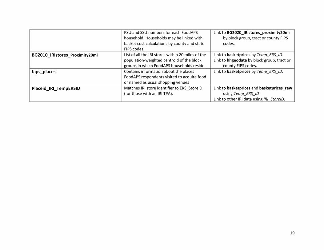
  19

PSU and SSU numbers for each FoodAPS household. Households may be linked with basket cost calculations by county and state FIPS codes 

Link to BG2020_IRIstores_proximity20mi by block group, tract or county FIPS codes.   

BG2010_IRIstores_Proximity20mi  List of all the IRI stores within 20 miles of the population‐weighted centroid of the block groups in which FoodAPS households reside. 

Link to basketprices by Temp_ERS_ID.  Link to hhgeodata by block group, tract or 

county FIPS codes.   

faps_places  Contains information about the places FoodAPS respondents visited to acquire food or named as usual shopping venues 

Link to basketprices by Temp_ERS_ID. 

Placeid_IRI_TempERSID  Matches IRI store identifier to ERS_StoreID (for those with an IRI TPA). 

Link to basketprices and basketprices_raw using Temp_ERS_ID 

Link to other IRI data using IRI_StoreID.  

 

   

  20

Table 2. Thrifty Food Plan Categories and Weights, Family of Four 

TFPNum  Food Type  Food Category 

Pounds Per Week: Males age 19‐50 

Pounds Per Week: Females age 19‐50 

Pounds Per Week: Child age 6‐8 

Pounds Per Week: Child age 9‐11 

1.1  Grains Whole grain bread, rice, pasta, pastries (incl whole grain flours)  2.82  1.25  0.9  1.7 

1.2  Grains  Whole grain cereals incl hot cereal mixes  0.08  0.38  .09  .07 

1.3  Grains  Popcorn and other whole grain snacks  0  0  .22  0 

1.4  Grains Non‐whole grain breads, cereal, rice, pasta, pies, pastries, snacks, and flours  1.66  1.14  1.19  .76 

2.1  Vegetables  All potato products  2.48  2.05  .29  1.07 

2.2  Vegetables  Dark green vegetables  1.24  1.29  .81  2.38 

2.3  Vegetables  Orange vegetables  0.98 1.19  .52  2.4 

2.4  Vegetables  Canned and dry beans, lentils, and peas or legumes  1.87  .93  .89  1.2 

2.5  Vegetables  Other vegetables  2.7  1.94  2.66  2.69 

3.1  Fruit  Whole fruit  6.65  5.16  2.8  3.97 

3.2  Fruit  Fruit juices  1.76  .46  1.82  1.86 

4.1  Milk products  Whole milk, yogurt, and cream  0.55  .2  .41  .97 

4.2  Milk products  Low‐fat and skim milk and low‐fat yogurt  10.75  11.31  7.2  10.81 

4.3  Milk products  All cheese, incl cheese soups and sauces  0.07  .03  .02  .01 

4.4  Milk products  Milk drinks and milk desserts  0  0  .06  0 

5.1  Meat and beans  Beef, pork, veal, lamb, and game  0.63  .65  1.25  .99 

5.2  Meat and beans  Chicken, turkey, and game birds  2.55  2.67  .33  .49 

5.3  Meat and beans  Fish and fish products  0.17  .43  .24  .46 

5.4  Meat and beans  Bacon, sausage, and lunch meats including spreads  0.02  0  .12  .01 

5.5  Meat and beans  Nuts, nut butters, and seeds  0.26  .47  .26  .43 

5.6  Meat and beans  Egg and egg mixtures  0.36  .06  .17  .28 

6.1  Other foods  Table fats, oils, and salad dressings  0.99  .55  .21  .36 

6.2  Other foods  Gravies, sauces, condiments, and spices  0.99  .55  .65  .53 

6.3  Other foods  Coffee and tea  0.01  .02  0  0 

  21

Source: 2006 Thrifty Food Plan report (CNPP, 2006) 

   

6.4  Other foods Soft drinks, sodas, fruit drinks, and ades incl rice beverages  0  0  .16  .02 

6.5  Other foods  Sugars, sweets, and candies  0.08  .04  .03  .02 

6.6  Other foods  Soups (ready‐to‐serve and condensed)  0.16  .76  .29  .16 

6.7  Other foods  Soups (dry)  0.02  0  .01  0 

6.8  Other foods Frozen/refrigerated entrees incl pizza, fish sticks, and frozen meals  0.01  0  .02  .01 

  22

Table 3. Product Hierarchy Example 

DeptID  Frozen 

Aisle  Frozen Meals 

Category  Breakfast Food – FZ 

Product  Bagel 

Type  Sesame 

 

   

  23

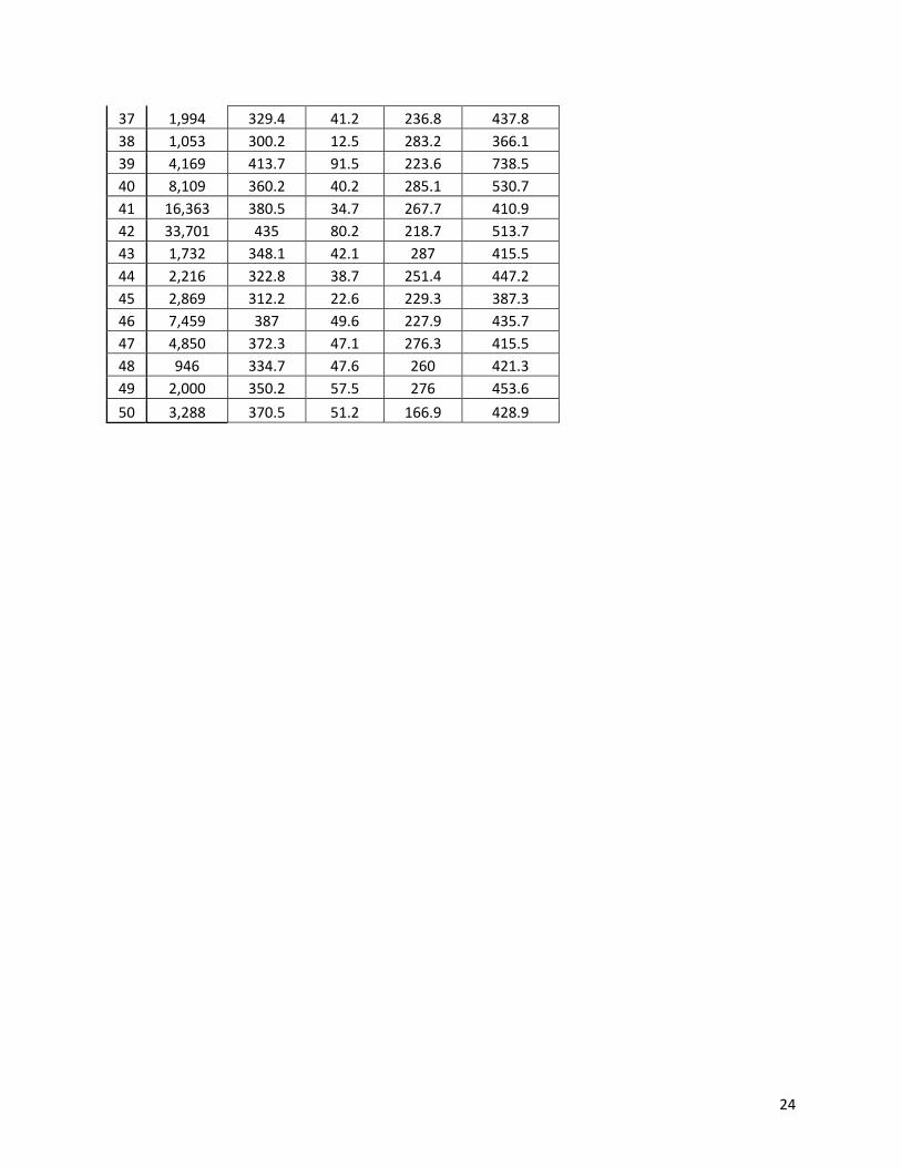
Table 4. Summary Statistics of Store‐Week Median Basket Costs, Including Only Store‐Weeks with Values for All 29 Food Categories 

PSU N=Store‐Weeks 

Basket Cost Using Median Category  Price Per Lb 

Average  Std Dev  Min  Max 

1  2,192  344.2  60.2  228.7  469.1 

2  3,003  305.2  28  230.6  410.1 

3  29,055  431.6  81.1  217.6  513.7 

4  1,451  309.9  21.5  230  352.7 

5  1,328  310.4  29.4  162.6  447.5 

6  742  326.3  43.8  295.3  429 

7  4,351  341.2  35.2  285.9  424.8 

8  1,842  324.5  26.9  287  377.8 

9  7,527  334.5  44.5  168.2  437.8 

10  2,381  344.1  37  292.4  397.3 

11  12,149  367.1  63.9  228.8  469.1 

12  5,087  372.1  44.3  291.5  414.8 

13  464  333.6  35.1  288.3  396.1 

14  824  299.3  25.2  227.1  325.2 

15  845  313.5  37.4  256.9  429 

16  3,005  370.4  45.4  291.5  441.7 

17  4,151  367.6  43.3  290.7  428.9 

18  4,428  379.2  48.4  278.4  575.5 

19  2,124  366.8  50.5  159.3  428.9 

20  1,236  306.6  24.5  222.7  371 

21  8,917  427.2  87.7  223.3  520.9 

22  15,515  363.3  60.4  148.7  459.5 

23  11,744  423.4  88.5  229.4  520.9 

24  10,822  379.7  75.6  231.7  658.5 

25  4,000  416.8  72.9  232  503.5 

26  1,711  399.3  76.8  228.2  477.6 

27  3,473  338.9  35.7  292  397.3 

28  11,971  377  64.2  245.2  454.4 

29  1,883  299.5  7.3  268.5  329.1 

30  583  310.5  7.1  298.3  325.2 

31  6,164  353  50.1  235.5  542.3 

32  4,759  425.3  85.7  223.6  738.9 

33  8,689  442.3  84.1  223.3  520.9 

34  2,958  356.3  44  167.9  402.5 

35  9,610  368  38.2  167.2  402.5 

36  689  311.5  16.9  283.3  359.7 

  24

37  1,994  329.4  41.2  236.8  437.8 

38  1,053  300.2  12.5  283.2  366.1 

39  4,169  413.7  91.5  223.6  738.5 

40  8,109  360.2  40.2  285.1  530.7 

41  16,363  380.5  34.7  267.7  410.9 

42  33,701  435  80.2  218.7  513.7 

43  1,732  348.1  42.1  287  415.5 

44  2,216  322.8  38.7  251.4  447.2 

45  2,869  312.2  22.6  229.3  387.3 

46  7,459  387  49.6  227.9  435.7 

47  4,850  372.3  47.1  276.3  415.5 

48  946  334.7  47.6  260  421.3 

49  2,000  350.2  57.5  276  453.6 

50  3,288  370.5  51.2  166.9  428.9 

   

  25

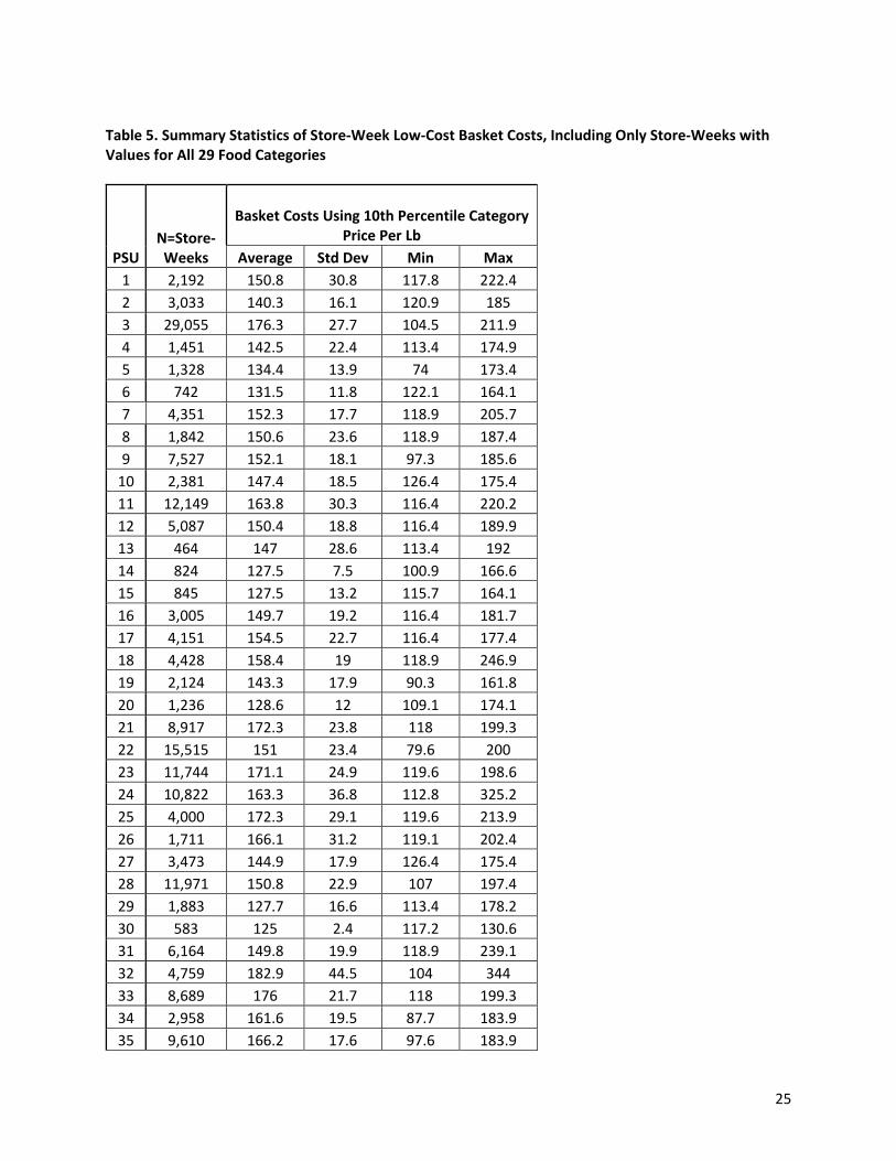
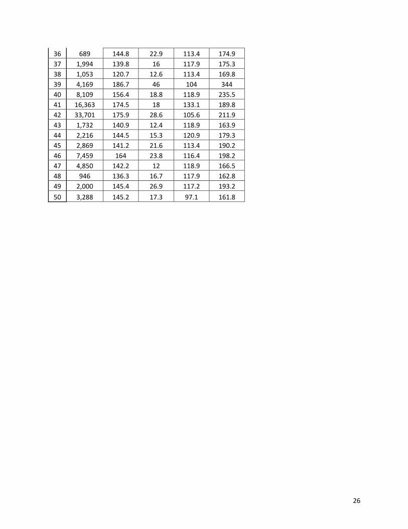
 Table 5. Summary Statistics of Store‐Week Low‐Cost Basket Costs, Including Only Store‐Weeks with Values for All 29 Food Categories  

PSU N=Store‐Weeks 

Basket Costs Using 10th Percentile Category Price Per Lb 

Average  Std Dev  Min  Max 

1  2,192  150.8  30.8  117.8  222.4 

2  3,033  140.3  16.1  120.9  185 

3  29,055  176.3  27.7  104.5  211.9 

4  1,451  142.5  22.4  113.4  174.9 

5  1,328  134.4  13.9  74  173.4 

6  742  131.5  11.8  122.1  164.1 

7  4,351  152.3  17.7  118.9  205.7 

8  1,842  150.6  23.6  118.9  187.4 

9  7,527  152.1  18.1  97.3  185.6 

10  2,381  147.4  18.5  126.4  175.4 

11  12,149  163.8  30.3  116.4  220.2 

12  5,087  150.4  18.8  116.4  189.9 

13  464  147  28.6  113.4  192 

14  824  127.5  7.5  100.9  166.6 

15  845  127.5  13.2  115.7  164.1 

16  3,005  149.7  19.2  116.4  181.7 

17  4,151  154.5  22.7  116.4  177.4 

18  4,428  158.4  19  118.9  246.9 

19  2,124  143.3  17.9  90.3  161.8 

20  1,236  128.6  12  109.1  174.1 

21  8,917  172.3  23.8  118  199.3 

22  15,515  151  23.4  79.6  200 

23  11,744  171.1  24.9  119.6  198.6 

24  10,822  163.3  36.8  112.8  325.2 

25  4,000  172.3  29.1  119.6  213.9 

26  1,711  166.1  31.2  119.1  202.4 

27  3,473  144.9  17.9  126.4  175.4 

28  11,971  150.8  22.9  107  197.4 

29  1,883  127.7  16.6  113.4  178.2 

30  583  125  2.4  117.2  130.6 

31  6,164  149.8  19.9  118.9  239.1 

32  4,759  182.9  44.5  104  344 

33  8,689  176  21.7  118  199.3 

34  2,958  161.6  19.5  87.7  183.9 

35  9,610  166.2  17.6  97.6  183.9 

  26

36  689  144.8  22.9  113.4  174.9 

37  1,994  139.8  16  117.9  175.3 

38  1,053  120.7  12.6  113.4  169.8 

39  4,169  186.7  46  104  344 

40  8,109  156.4  18.8  118.9  235.5 

41  16,363  174.5  18  133.1  189.8 

42  33,701  175.9  28.6  105.6  211.9 

43  1,732  140.9  12.4  118.9  163.9 

44  2,216  144.5  15.3  120.9  179.3 

45  2,869  141.2  21.6  113.4  190.2 

46  7,459  164  23.8  116.4  198.2 

47  4,850  142.2  12  118.9  166.5 

48  946  136.3  16.7  117.9  162.8 

49  2,000  145.4  26.9  117.2  193.2 

50  3,288  145.2  17.3  97.1  161.8 

    

  27

References  Broda, C., and D.E. Weinstein. 2010. “Product Creation and Destruction: Evidence and Price 

Implications.” American Economic Review 100: 697‐723. 

Center for Nutrition Policy and Promotion (CNPP) USDA. 2007. Thrifty Food Plan, 2006. 1‐64. 

Feenstra, R. C. 1994. “New Product Varieties and the Measurement of International Prices.” American 

Economic Review 84: 157‐157. 

Gundersen C., A. Satoh, A. Dewey, M. Kato, and E. Engelhard. Map the Meal Gap 2015:  Technical Brief.  

Feeding America.  2015. 

Handbury, J., and D.E. Weinstein. 2014. “Goods Prices and Availability in Cities.” The Review of Economic 

Studies 81(4): 1‐39. 

Hottman, C. 2014. “Retail Markups, Misallocation, and Store Variety in the US.” Department of 

Economics, Columbia University, U.S. 

Retail Planet 2008. Grocery Retailing in U.S.A. London: Planet Retail Ltd. 

Todd, J., L. Mancino, E. Leibtag, C. Tripodo. 2010. “Methodology Behind the Quarterly Food‐at‐Home 

Price Database”. The Economic Research Service, USDA, U.S. 

U.S. Department of Agriculture. 2015. Food Safety and Inspection Services. Shell Eggs from Farm to 

Table.