constructing multivariate simulation metamodels for supporting supply chain...

ISSN: 2306-9007 Winch, Kuei & Madu (2013)

728

Constructing Multivariate Simulation Metamodels for

Supporting Supply Chain Management

JANICE K. WINCH Department of Management and Management Science

Lubin School of Business Pace University New York, NY, USA

Email: [email protected]

Tel: +12126186564

CHU-HUA KUEI Department of Management and Management Science



CHRISTIAN N. MADU Department of Management and Management Science



Abstract This paper describes a multivariate simulation metamodeling approach for supporting supply chain

management. We use discrete event simulation to examine the links between controllable factors and the

supply chain performance. Based on the results of the simulation, regression metamodels are developed.

The resource allocation decision on the controllable factors is made by a linear programming model. The

paper also presents three modeling frameworks in which the metamodeling approach can be used. They

are the hierarchical model, the SCOR model and the integrated supply chain model. The simulation

metamodeling approach and the strategic modeling frameworks demonstrated in this paper will assist

supply chain managers in resource allocation decisions as they initiate and plan supply chain improvement

projects.

Key Words: Multivariate Simulation Metamodel, Supply Chain Management, Supply Chain Design, Supply

Chain Simulation Model, Taguchi Method.

Introduction

Supply Chain Management (SCM) has a profound effect on business practices and performance. As noted by

Chow et al. (2008), Madu and Kuei (2004), and Kuei, Madu, Lin, and Chow (2002), SCM is a holistic and

a strategic approach to demand, operations, procurement, and logistics management. Two observations

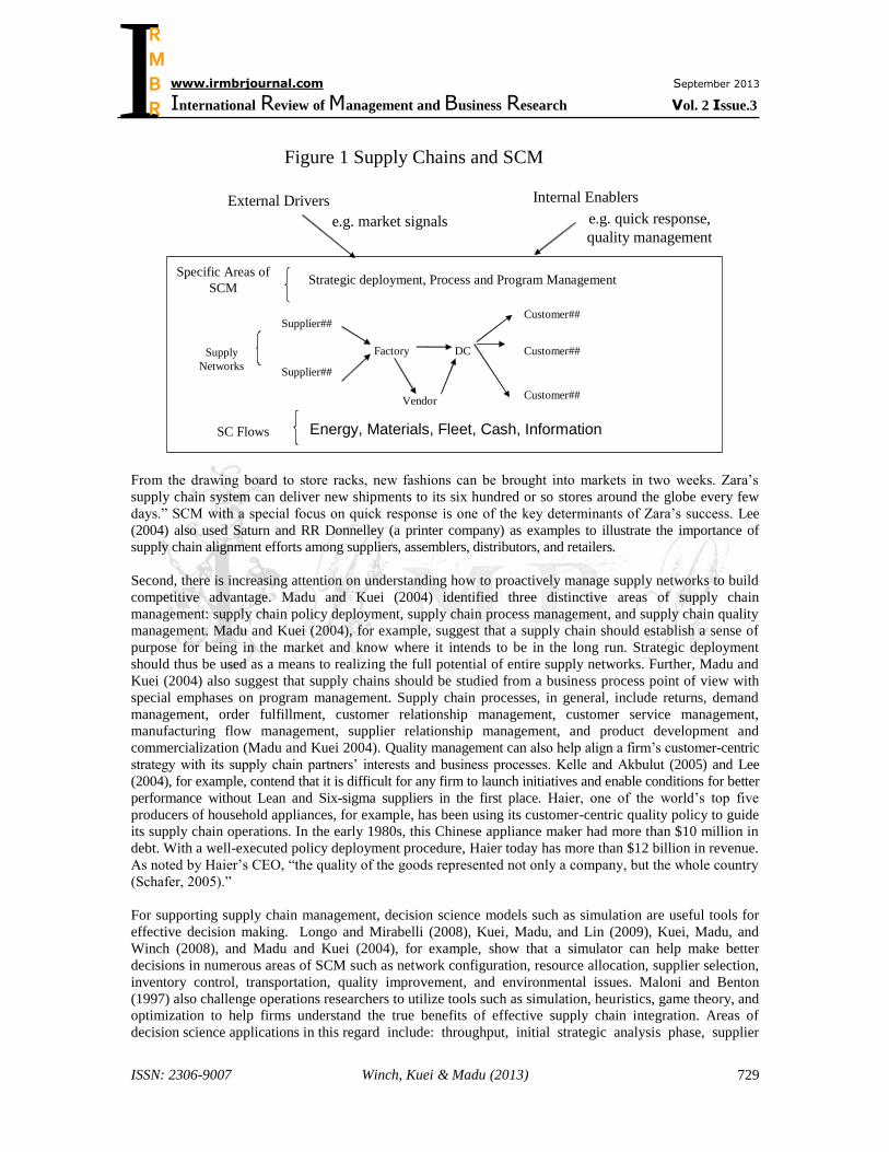
about SCM are depicted in Figure 1 and summarized here.

First, SCM seeks to respond to market demands correctly and profitably. Facing operations management

paradigm shifts, demand and supply uncertainties, and constant conflicts among supply chain units, listening to

market signals and synchronizing countermeasures is more important than ever. Market signals in this context

can be considered as external drivers of supply chain management design and practices, while

countermeasures such as quick response and quality management can be noted as internal enablers. Over the

past decade, industry leaders such as Zara (the Spanish apparel manufacturer and retailer), Nokia, Toyota,

Cisco, Microsoft, and Hewlett-Packard have adopted customer-centric supply chain initiatives and cross-

enterprise processes. As noted by Chow et al. (2008, p.666), for example, Zara “learned to introduce more

than 11,000 products per year.

I

www.irmbrjournal.com September 2013

International Review of Management and Business Research Vol. 2 Issue.3

R M B R

mailto:[email protected]



http://www.irmbrjournal.com/


729

Factory DC

Customer##

Customer##

Customer##Vendor

Supplier##

Supplier##

Figure 1 Supply Chains and SCM

SC Flows Energy, Materials, Fleet, Cash, Information

e.g. market signals

External Drivers

e.g. quick response,

quality management

Internal Enablers

Strategic deployment, Process and Program Management Specific Areas of

SCM

Supply

Networks

From the drawing board to store racks, new fashions can be brought into markets in two weeks. Zara’s

supply chain system can deliver new shipments to its six hundred or so stores around the globe every few

days.” SCM with a special focus on quick response is one of the key determinants of Zara’s success. Lee

(2004) also used Saturn and RR Donnelley (a printer company) as examples to illustrate the importance of

supply chain alignment efforts among suppliers, assemblers, distributors, and retailers.

Second, there is increasing attention on understanding how to proactively manage supply networks to build

competitive advantage. Madu and Kuei (2004) identified three distinctive areas of supply chain

management: supply chain policy deployment, supply chain process management, and supply chain quality

management. Madu and Kuei (2004), for example, suggest that a supply chain should establish a sense of

purpose for being in the market and know where it intends to be in the long run. Strategic deployment

should thus be used as a means to realizing the full potential of entire supply networks. Further, Madu and

Kuei (2004) also suggest that supply chains should be studied from a business process point of view with

special emphases on program management. Supply chain processes, in general, include returns, demand

management, order fulfillment, customer relationship management, customer service management,

manufacturing flow management, supplier relationship management, and product development and

commercialization (Madu and Kuei 2004). Quality management can also help align a firm’s customer-centric

strategy with its supply chain partners’ interests and business processes. Kelle and Akbulut (2005) and Lee

(2004), for example, contend that it is difficult for any firm to launch initiatives and enable conditions for better

performance without Lean and Six-sigma suppliers in the first place. Haier, one of the world’s top five

producers of household appliances, for example, has been using its customer-centric quality policy to guide

its supply chain operations. In the early 1980s, this Chinese appliance maker had more than $10 million in

debt. With a well-executed policy deployment procedure, Haier today has more than $12 billion in revenue.

As noted by Haier’s CEO, “the quality of the goods represented not only a company, but the whole country

(Schafer, 2005).”

For supporting supply chain management, decision science models such as simulation are useful tools for

effective decision making. Longo and Mirabelli (2008), Kuei, Madu, and Lin (2009), Kuei, Madu, and

Winch (2008), and Madu and Kuei (2004), for example, show that a simulator can help make better

decisions in numerous areas of SCM such as network configuration, resource allocation, supplier selection,

inventory control, transportation, quality improvement, and environmental issues. Maloni and Benton

(1997) also challenge operations researchers to utilize tools such as simulation, heuristics, game theory, and

optimization to help firms understand the true benefits of effective supply chain integration. Areas of

decision science applications in this regard include: throughput, initial strategic analysis phase, supplier

I



R M B R



730

selection and evaluation phase, partnership establishment phase, and maintenance phase. Kelle and Akbulut

(2005) also provide a literature review on quantitative support for supply chain optimization. Through the use

of quantitative models, supply chain relationships, either in the form of partnership or adversarial relationship,

can be quantified and evaluated in terms of costs and benefits. Two main results from their quantitative

analyses are:

The joint optimal policy will always benefit the entire supply chain.

Coordinating the safety stock policy will always result in cost savings.

In addition, Madu and Kuei (2004) employ linear programming (LP) models for the postponement decisions.

Monte Carlo simulations for assessing inventory policy and behavior during early-sales period are also

discussed.

In this paper, we show how a combination of simulation-based metamodeling and linear programming can

be used to improve supply chain decisions. We first identify the specific relationships between controllable

factors and performance outcomes in a supply chain simulation setting through using the metamodeling

approach. Then we formulate a linear programming model with these relationships and solve it to find the

optimal supply chain design. This paper is organized as follows. In the next section, we focus on earlier

research on critical aspects of supply chain systems and regression metamodeling in computer simulation.

In section 3 we illustrate our modeling approach and results. In section 4 we discuss frameworks for

potential applications and follow with conclusions in section 5.

Research Background

Past Work on Modeling Supply Chain Systems

The subject of simulation modeling approaches for complex supply chain systems has received

considerable interest in the literature. Bottani and Montanari (2009), for example, use discrete-event

simulation models to understand the behavior of a fast moving consumer goods supply chain and optimize

supply chain design. In their simulation study, thirty supply chain configurations were tested for logistical

costs and the demand variance. Major parameters adopted by Bottani and Montanari (2009) include (a)

numbers of echelons (from three to five), (b) inventory policies (EOQ or economic order interval ( EOI)),

(c) information sharing mechanisms (absence or presence of such a mechanism), (d) daily final customer’s

demand values and behavior, and (e) the responsiveness of supply chain players. Three supply chain flows

such as product, order, and information are also noted in the supply chain simulation model.

In a similar fashion, Zhang and Zhang (2007) propose a supply chain simulation model with four different

supply chain performance measures. They are service, inventory cost, backlog cost, and total cost. Major

experimental settings center on demand variance and location of distributor in China. Rabelo, Eskandari,

Shaalan, and Helal (2007) present a hybrid approach that integrates system dynamics, discrete-event

simulation, and the Analytic Hierarchy Process (AHP) to model the service and manufacturing activities of

a multinational construction equipment firm’s global supply chain.

Longo and Mirabelli (2008) also contend that a parametric supply chain simulator is a decision making tool

capable of analyzing different supply chain scenarios. Major parameters considered by Longo and

Mirabelli (2008) include inventory policies, lead times, and customers’ demand intensity and variability.

Three supply chain nodes such as stores, distribution centers, and plants are presented. Their simulation

models were tested for three supply chain performance measures: fill rate, on hand inventory, and inventory

costs. Metamodels, or statistical models used to express Y (i.e., dependent variable such as fill rate) as

function of ix (i.e., independent variables or factors such as inventory policies, lead times, and customers’

demand) are also constructed by Longo and Mirabelli (2008) for each performance measure.

Both Kuei, Madu, and Winch (2008) and Shang, Li, and Tadikamalla (2004) elaborate on the use of

Taguchi design and metamodeling approaches to model a relatively complex supply chain network. L16

Taguchi design is used by Kuei et al. (2008).

I



R M B R



731

Shang et al. (2004) choose L27 Taguchi design for controllable factors. Chwif, Barretto, and Saliby (2002)

compare spreadsheet-based and simulation-based tools in the analysis of a supply chain system. They conclude

that discrete event simulation is the right tool when conducting in-depth supply chain analyses. Jain, Lim, Gan,

and Low (1999) used simulation to study the behavior of supply chain networks and were able to identify

logistics and business processes as the two major issues surround such networks. Towill, Naim, and Wikner

(1992) compared different quick-response-to-orders strategies based on a supply chain simulation model.

The aforementioned studies illustrate how simulation models have been used to assess the impact of

controllable factors on supply chain performances under various supply chain configurations. In this paper,

the data generated by the simulation models are used to build regression metamodels that explicitly

describe such relationships.

Regression Metamodeling in Computer Simulation

Longo and Mirabelli (2008), Kuei et al. (2008), Friedman and Pressman (1988), and Madu and Kuei (1993,

1994) offer a comprehensive review on regression metamodeling in computer simulation. As reported by Kuei

et al. (2008, p.135) and Friedman and Pressman (1988), “the benefits of constructing a metamodel in a

simulation study include model simplification, enhanced exploration and interpretation of the model generation

to other models of the same type, sensitivity analyses, optimization, answering inverse questions, and providing

the researcher with a better understanding of the behavior of the system under study.” When developing

metamodels, researchers and decision makers need to consider the following three issues: establishing the

mathematical form of metamodel, preparing full or fractional factorial design plans, and conducting single-

stage or multiple-stage experiments. In the following, we shall briefly discuss these three issues.

(1) Establishing the mathematical form of metamodel

If we assume that the simulation model yields a system performance Y equal to the additive effects of the inputs

( 1, , ),ix i k then

0

1

k

i i

i

Y x e (1)

where 0

is the grand mean; iis the coefficient of single factor i; and e is the experimental error. If we

assume that the simulation input factors also interact, then we have a second-order regression model

0

1 2

k k k

i i ij i j

i i j j

Y x x x e (2)

where ij

denotes the coefficient of the interaction between group factors i and j. This is the form adopted by

Kuei et al. (2008). More complicated forms and models can be found in Longo and Mirabelli (2008) and

Shang et al. (2004). Other examples of using regression metamodels for decision making appear in Kumar,

Satsangi, and Prajapati (2013) and Winch, Madu, and Kuei (2012). Kumar, et al. (2013) use second-order

metamodels to minimize casting defect in a melt shop industry. Winch et al. (2012) illustrate how

metamodeling combined with goal programming can be used to minimize operational cost and waste in a

reverse logistics system.

(2) Preparing full or fractional factorial design plans

As noted by Shang et al. (2004, p.3835), an ideal experimental design plan “provides the maximum amount

of information with the minimum number of trials. Taguchi developed orthogonal arrays, linear graphs, and

triangular tables to reduce the experiment time and to increase accuracy.” If decision makers need to

consider five factors, for example, at two levels each, then the total number of factor combinations is 25, or 32.

In other words, thirty two simulation runs are expected if this full factorial design is adopted. When the full

factorial plan is executed, higher-order interactions such as three-factor interaction can be estimated. However,

in many situations, this plan is too expensive and impracticable since high-order interactions are often

insignificant (Kuei et al. 2008).

I



R M B R



732

If decision makers can assume that the higher-order interactions are not significant, then they can adopt

fractional factorial design plans. With the same five input factors, that means only 25-1

, or 16 simulation runs are

required. In a Taguchi design, decision makers can set up the fractional factorial design plan based on the L16

orthogonal arrays and the corresponding linear graphs (Kuei et al. 2008, Madu and Kuei 1993, Peace 1993,

Taguchi and Wu 1980). Shang et al. (2004), referring to Taguchi’s orthogonal array tables, choose the L27

design for controllable factors such as reliability, capacity, lead time, reorder quantity, information sharing,

and delayed differentiation in their simulation study. To examine the effects of these six controllable

factors, at three levels each, then the total number of factor combinations is 36, or 729. Using the Taguchi

method, only 27 experiments are required.

(3) Conducting Single-stage or Multiple-stage Experiments

As noted by Kuei et al. (2008) and Madu and Kuei (1993, 1994), if the number of simulation input factors is

small (say 5k ), a single-stage approach is sufficient when constructing metamodels. This approach is

adopted by both Longo and Mirabelli (2008) and Shang et al. (2004). When many input factors are

considered (e.g., 5k ), however, multiple-stage experiments are more appropriate. As noted by Kuei et al.

(2008), it is unwise to investigate all the controllable factors in the initial stage of an experiment. In some

situations, individual factors can also be aggregated into groups. With a large number of input factors and/or

group factors, the attempt should center on screening experimentation and identifying the most important

(individual and/or group) factors. In the follow-up experiment, single factors and any group factors of interest

can be further tested and investigated. With the exception of a few recent studies, little work of any depth has

been published on the multiple-stage experimentation in a supply chain setting. In this simulation study, we

will follow the multiple-stage experimentation procedure outlined by Kuei et al. (2008) and Madu and Kuei

(1994).

Metamodeling and Optimizing a Supply Chain Network

Problem Setting

With the aim of analyzing a supply chain system through using simulation modeling approaches, we need to

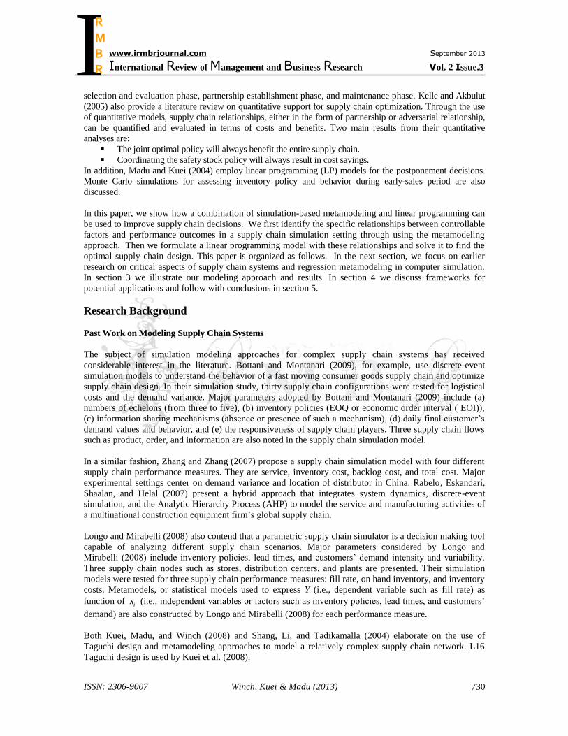
first frame the issues and define our problem. For the purpose of this study, we consider a single laptop

computer supply chain network operating with one distribution center and two customer zones (see Figure 2).

Distribution

Center

Market 1

Monitor

Keyboard

Power Supply

Figure 2 Supply Chain Networks

Market 2

The distribution center purchases monitors, keyboards, and power supply modules from three supply

groups. The final assembly is done in the distribution center. End user orders from those two customer

zones are consolidated in the order fulfillment office. They are fulfilled subsequently by the distribution

center. The supply chain system described here is in line with that of Longo and Mirabelli (2008) and

Towers and Burnes (2008). For example, lead time management is considered by Towers and Burnes

(2008) as one of the primary strategic and operational requirements in a supply chain setting.

I



R M B R



733

We want to see how the overall lead time for the customer is related to the intermediate lead times within

the supply chain network and perhaps the time to repair defective items, if any. With all time units in

hours, the definitions of both the dependent and input variables in our first stage of experimentation are

given below. The assumed distributions with their parameters for the input variables are shown in Table 1.

Dependent variables:

LTime (Market 1): average lead time needed for the first customer zone

LTime (Market 2): average lead time needed for the second customer zone

Input variables:

Demand (Market 1): the variation of demand in the first customer zone

Demand (Market 2): the variation of demand in the second customer zone

DCTR LTime: lead time between the distribution center and customer zones

Supply Group LTime: lead time between supply groups and the distribution center

MTTR: Mean Time to Repair

Table 1 Original Data

Demand Lead Time MTTR

Market 1 - Demand N(60,12)

Market 2 - Demand EXP(60)

Distribution Center EXP(48) EXP(48)

Power Supply EXP(60)

Monitor EXP(48)

Keyboard EXP(48)

N(mean, standard deviation): Normal Distribution

EXP(MTTR): Exponential Dist (Mean Time to Repair)

All time units are in hours.

The primary assumptions of the supply chain model here are summarized as follows:

End user orders from the first customer zone are consolidated and follow the normal distribution.

End user orders from the second customer zone are consolidated and follow the exponential

distribution.

The lead time between the distribution center and two customer zones follows the exponential

distribution.

The lead time between the distribution center and suppliers follows the exponential distribution.

At the distribution center, the defective rate for the first customer zone’s orders is ten percent.

The defective items are repairable and are assumed to be completely rejuvenated after each repair.

The repair time follows the exponential distribution.

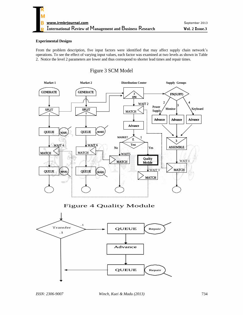
Simulation Model

The simulation model for the described supply network setting is shown in Figure 3. This model was coded in

GPSS/H for our experiments. As can be seen in Figure 3, there are four major segments and one module in the

simulation model. The first two segments represent market demands and customer orders. The third segment

represents the operation of the distribution center. The fourth segment depicts the operations of three supply

groups and the assembly process in the distribution center. The quality module (see Figure 4) is included in the

third segment to simulate the failure and repair processes.

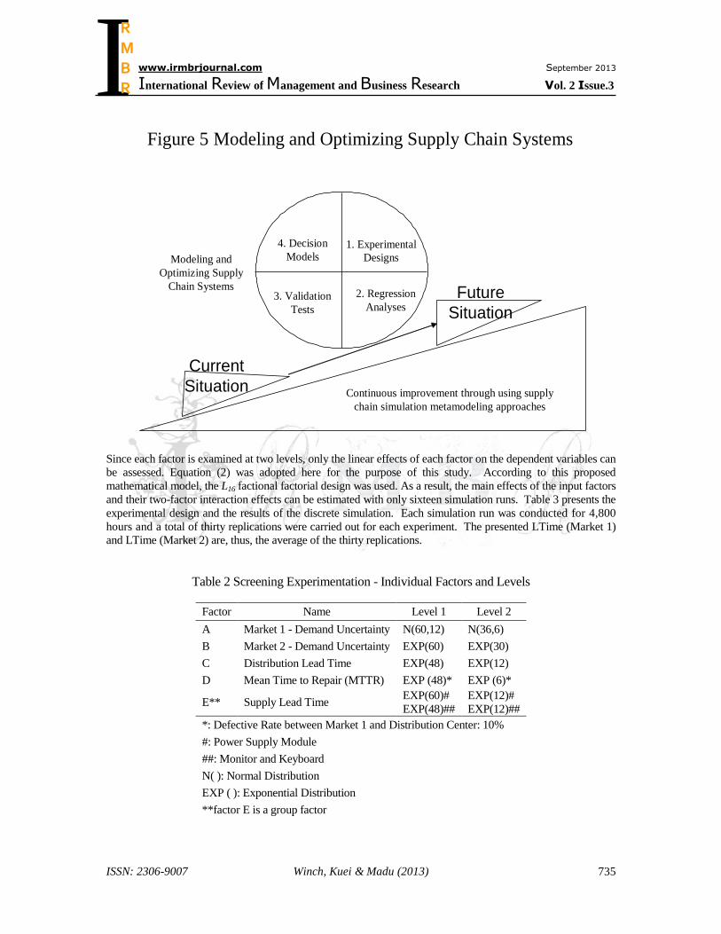
In the remainder of section, we describe a sequential procedure for utilizing the simulation results to construct

and apply regression metamodels (see Figure 5). This new cycle of modeling and optimizing supply chain

systems involves four steps: experimental designs, regression analyses, validation tests, and decision models.

I



R M B R



734

Experimental Designs

From the problem description, five input factors were identified that may affect supply chain network’s

operations. To see the effect of varying input values, each factor was examined at two levels as shown in Table

2. Notice the level 2 parameters are lower and thus correspond to shorter lead times and repair times.

Figure 3 SCM Model

Distribution Center Supply Groups

WAIT 1

Market 1 Market 2

1

SPLIT

QUEUE

MATCH

MAR1

GENERATE

WAIT 4

MAR1QUEUE

1

SPLIT

QUEUEQUEUE

MATCHMATCH

MAR1MAR1

GENERATEGENERATE

WAIT 4

MAR1MAR1QUEUEQUEUE WAIT 3

Test

EMARKET 1

Yes

Advance

3

1PH

WAIT 2

WAIT5

MATCH

MATCH

Quality

ModuleMATCH

NoTest

EMARKET 1

Yes

AdvanceAdvance

3

1PH

3

1PH

WAIT 2

WAIT5

MATCH

MATCHMATCH

Quality

Module

Quality

ModuleMATCHMATCH

No

1

SPLIT

QUEUE

GENERATE

WAIT 6

MATCH

MAR2

MAR2QUEUE

1

SPLIT1

SPLIT

QUEUEQUEUE

GENERATEGENERATE

WAIT 6

MATCH

MAR2MAR2

MAR2MAR2QUEUEQUEUE

Power

SupplyMonitor Keyboard

2 4

3

ASSEMBLE

FN(SUPP)

MATCH

Advance Advance Advance

3Power

SupplyMonitor Keyboard

2 4

3

ASSEMBLE

3

ASSEMBLE

FN(SUPP)FN(SUPP)

MATCHMATCH

Advance Advance AdvanceAdvanceAdvance AdvanceAdvance AdvanceAdvance

3

QUEUEQUEUE

QUEUEQUEUE

RepairRepair

RepairRepair

AdvanceAdvance

Transfer

.1

.1

Figure 4 Quality Module

I



R M B R



735

1. Experimental

Designs

2. Regression

Analyses3. Validation

Tests

4. Decision

ModelsModeling and

Optimizing Supply

Chain Systems

Figure 5 Modeling and Optimizing Supply Chain Systems

Future

Situation

Current

Situation Continuous improvement through using supply

chain simulation metamodeling approaches

Since each factor is examined at two levels, only the linear effects of each factor on the dependent variables can

be assessed. Equation (2) was adopted here for the purpose of this study. According to this proposed

mathematical model, the L16 factional factorial design was used. As a result, the main effects of the input factors

and their two-factor interaction effects can be estimated with only sixteen simulation runs. Table 3 presents the

experimental design and the results of the discrete simulation. Each simulation run was conducted for 4,800

hours and a total of thirty replications were carried out for each experiment. The presented LTime (Market 1)

and LTime (Market 2) are, thus, the average of the thirty replications.

Table 2 Screening Experimentation - Individual Factors and Levels

Factor Name Level 1 Level 2

A Market 1 - Demand Uncertainty N(60,12) N(36,6)

B Market 2 - Demand Uncertainty EXP(60) EXP(30)

C Distribution Lead Time EXP(48) EXP(12)

D Mean Time to Repair (MTTR) EXP (48)* EXP (6)*

E** Supply Lead Time EXP(60)#

EXP(48)##

EXP(12)#

EXP(12)##

*: Defective Rate between Market 1 and Distribution Center: 10%

#: Power Supply Module

##: Monitor and Keyboard

N( ): Normal Distribution

EXP ( ): Exponential Distribution

**factor E is a group factor

I



R M B R



736

Table 3 Screening Experimentation - Systematic Assignment to Five Factors and Multivariate Simulation

Results

Factor

A

Factor

B

Factor

C

Factor

D

Factor

E

Avg. LTime

(M1)

Avg. LTime

(M2)

1 Level 1 Level 1 Level 1 Level 1 Level 1 145.10 139.82
















LTime is in hours. M1 = Market 1, M2 = Market 2

The analysis of variance (ANOVA) procedure was applied to test the significance of both the main and two-

factor interaction effects (Kuei et al. 2008, Longo and Mirabelli 2008). The ANOVA tests in Table 4 show that

factors C (DCTR LTime) and E (Supply Group LTime) are statistically significant at α = 0.01. Notice that

factor E is a group factor. Notice also that the “pooling” technique is employed to estimate the experimental

error. For example, for the case of LTime (M1), since the sum of squares (SS) values of factor A, factor B,

factor D, and all the two-factor interactions are very small, they are aggregated and used to estimate the

experimental error.

Table 4 ANOVA Results

Avg. LTime (M1) Avg. LTime (M2)

Source SS MS F SS MS F

Factor A 97 71

Factor B 65 88

Factor C 3695 3695 43.06# 3717 3717 42.75#

Factor D 262 107

Factor E 18531 18531 215.98# 17996 17996 206.97#

A * B 51 81

A * C 63 70

B * C 105 76

D * E 96 63

A * D 60 98

B * D 59 67

C * E 64 57

C * D 67 119

B * E 54 90

A * E 72

143

Pool Error: 86 87

#: At least 99% confidence

I



R M B R



737

Given the new information about our initial experimental factors, in the follow-up experiment, we consider the

following five factors:

DCTR LTime: lead time between the distribution center and customer zones

PSM LTime: lead time between our Power Supply Module group and the distribution center

Monitor LTime: lead time between our Monitor group and the distribution center

Keyboard LTime: lead time between our Keyboard group and the distribution center

MTTR: Mean Time to Repair (the defective rates at the supply groups and the distribution center are

identical in the follow-up experiment)

The levels used are shown in Table 5. The L16 factional factorial design plan and simulation results are shown

in Table 6. Table 7 shows the results based on the ANOVA test. It turns out that all experimental factors in the

follow-up experiment are significant at α = 0.01.

Table 5 Follow-up Experimentation - Individual Factors and Levels

Factor Name Level 1 Level 2

A Distribution Lead Time EXP(48) EXP(12)

B Power Supply Lead Time EXP(60) EXP(12)

C Monitor Supply Lead Time EXP(48) EXP(12)

D Keyboard Supply Lead Time EXP(48) EXP(12)

E Distribution and Supply Group’s MTTR EXP (48) EXP (6)

EXP ( ): Exponential Distribution

Table 6 Follow-up Experimentation - Systematic Assignment to Five Factors and Multivariate Simulation

Results

Factor A Factor B Factor C Factor D Factor E Avg. LTime

(M1)

Avg. LTime

(M2)

















M1: Market 1’s Average Lead Time (Hours); M2: Market 2’s Average Lead Time (Hours)

I



R M B R



738

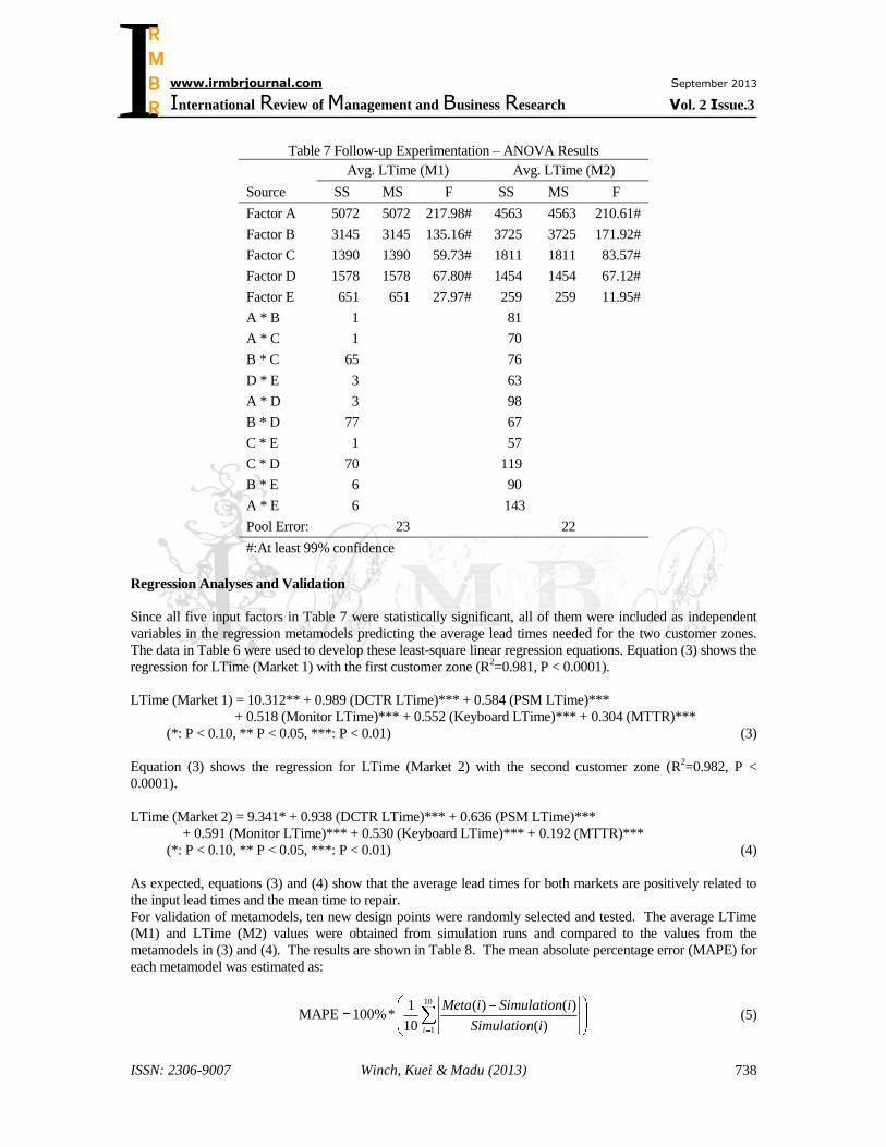
Table 7 Follow-up Experimentation – ANOVA Results

Avg. LTime (M1) Avg. LTime (M2)

Source SS MS F SS MS F

Factor A 5072 5072 217.98# 4563 4563 210.61#

Factor B 3145 3145 135.16# 3725 3725 171.92#

Factor C 1390 1390 59.73# 1811 1811 83.57#

Factor D 1578 1578 67.80# 1454 1454 67.12#

Factor E 651 651 27.97# 259 259 11.95#

A * B 1 81

A * C 1 70

B * C 65 76

D * E 3 63

A * D 3 98

B * D 77 67

C * E 1 57

C * D 70 119

B * E 6 90

A * E 6 143

Pool Error: 23 22

#:At least 99% confidence

Regression Analyses and Validation

Since all five input factors in Table 7 were statistically significant, all of them were included as independent

variables in the regression metamodels predicting the average lead times needed for the two customer zones.

The data in Table 6 were used to develop these least-square linear regression equations. Equation (3) shows the

regression for LTime (Market 1) with the first customer zone (R2=0.981, P < 0.0001).

LTime (Market 1) = 10.312** + 0.989 (DCTR LTime)*** + 0.584 (PSM LTime)***

+ 0.518 (Monitor LTime)*** + 0.552 (Keyboard LTime)*** + 0.304 (MTTR)***

(*: P < 0.10, ** P < 0.05, ***: P < 0.01) (3)

Equation (3) shows the regression for LTime (Market 2) with the second customer zone (R2=0.982, P <

0.0001).

LTime (Market 2) = 9.341* + 0.938 (DCTR LTime)*** + 0.636 (PSM LTime)***

+ 0.591 (Monitor LTime)*** + 0.530 (Keyboard LTime)*** + 0.192 (MTTR)***

(*: P < 0.10, ** P < 0.05, ***: P < 0.01) (4)

As expected, equations (3) and (4) show that the average lead times for both markets are positively related to

the input lead times and the mean time to repair.

For validation of metamodels, ten new design points were randomly selected and tested. The average LTime

(M1) and LTime (M2) values were obtained from simulation runs and compared to the values from the

metamodels in (3) and (4). The results are shown in Table 8. The mean absolute percentage error (MAPE) for

each metamodel was estimated as:

10

1

1 ( ) ( )MAPE 100%*

10 ( )i

Meta i Simulation i

Simulation i (5)

I



R M B R



739

where Meta(i) = output value from the metamodel in experiment i, and Simulation(i) = output value from the

simulation in experiment i. The MAPEs of 2.9% and 3.7% were observed for our two regression metamodels

respectively. We therefore conclude that the metamodel is valid in estimating the response lead times in both

customer zones.

Table 8 Validation Test for LTime (M1) and LTime (M2)

LTime (M1) LTime (M2)

A B C D E Simulation Metamodel %

Error Simulation Metamodel

%

Error

1 38 55 19 22 40 113.54 114.16 0.5% 109.63 110.53 0.8%

2 42 26 39 35 38 113.70 118.11 3.9% 111.59 114.17 2.3%

3 20 34 42 37 17 93.78 97.30 3.7% 92.09 97.42 5.8%

4 18 15 35 42 29 83.94 87.00 3.7% 82.56 84.28 2.1%

5 33 28 41 16 19 93.80 95.15 1.4% 88.99 94.46 6.1%

6 45 45 15 19 38 110.44 110.91 0.4% 103.64 106.40 2.7%

7 25 51 24 31 42 103.66 107.13 3.4% 101.52 103.91 2.3%

8 16 16 36 42 36 85.63 88.26 3.1% 82.64 84.97 2.8%

9 29 38 28 26 22 91.18 96.73 6.1% 87.64 95.26 8.7%

10 34 42 14 15 25 89.49 91.60 2.4% 86.28 88.97 3.1%

MAPE 2.9% MAPE 3.7%

Decision Model

The essence of optimizing supply chain systems is to find the best solution for a given objective. At this point,

we have a good sense about which areas in our supply networks should be targeted for improvement. Our next

task is centered on resource allocation. Suppose the goal is to decrease the average response time in the first

market to 100 hours (the current response time is 151.39 hours in the first market). Given that improving the

supply chain speed requires additional investment, we wish to satisfy this requirement at the minimum

additional cost. The specifics of the investment areas and possibilities are shown in Table 9. Here, we can use

the linear programming solution approach to minimize the cost of improving supply chain speed for market 1.

Notice that there are two set of decision variables: iX represents the individual factor or area, while

iY is

defined as the number of units (levels) that each factor or area could be improved (i = A, B, C, D, and E).

Notice that equation (3) is incorporated in our linear programming model for the supply chain speed

computation. Note also that we move the constant 10 from the left-hand side to the right-hand side (For

simplicity, we use 10, instead of 10.312). The marginal improvement cost (MIC) can also be found in Table 9.

Table 9 Original Data - Decision Model

Facto

r

Normal

Scenario

(NS)

Best

Scenario

(BS)

Maximum

Reduction

(MR=NS-

BS)

Normal

Cost

(NC)

Cost for

the BS

(CBS)

Extra

Cost

(EC=CBS-

NC)

Marginal

Improvement

Cost

(MIC=EC/MR)

A 48 12 36 $100 $280 $180 $5.0

B 60 12 48 $50 $98 $48 $1.0

C 48 12 36 $40 $94 $54 $1.5

D 48 12 36 $40 $76 $36 $1.0

E 48 6 42 $10 $31 $21 $0.5

The factors are as defined in Table 5. Time units are in hours and cost units are in $thousands.

I



R M B R



740

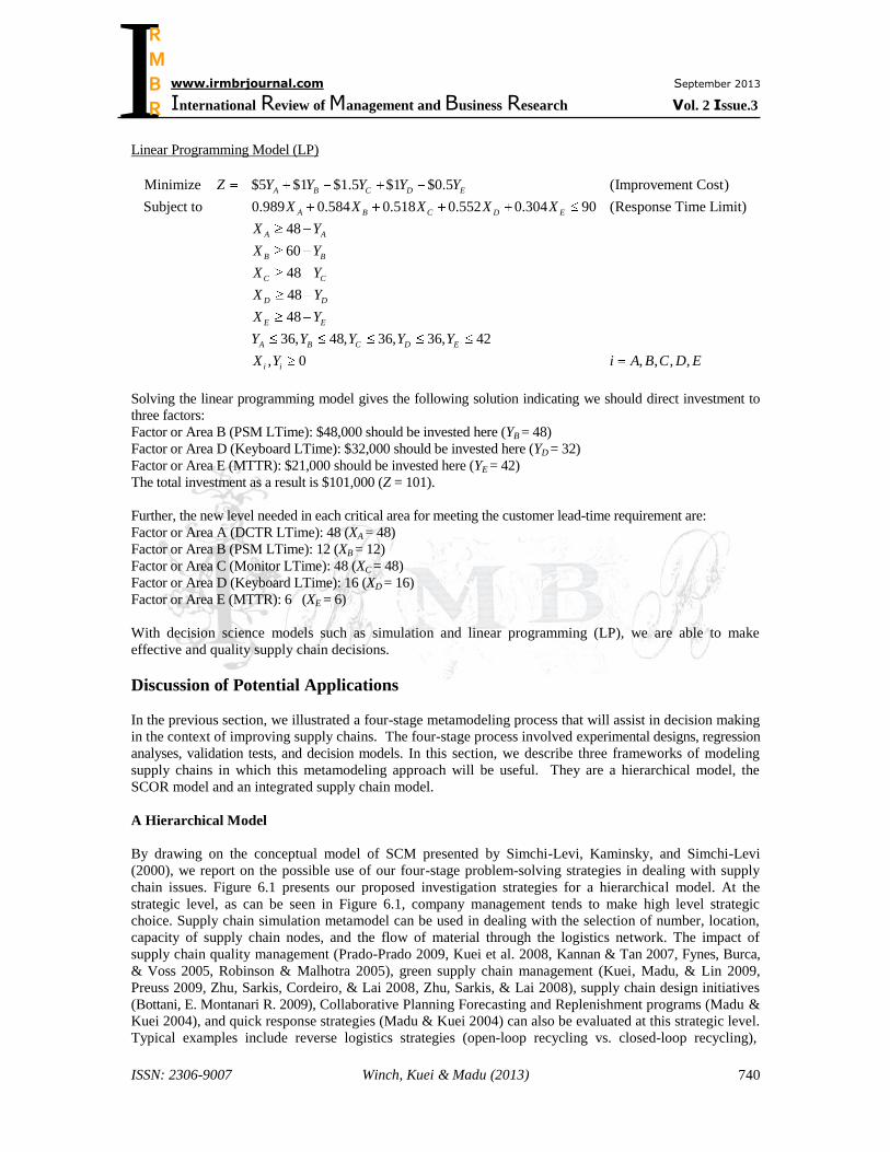
Linear Programming Model (LP)

Minimize $5 $1 $1.5 $1 $0.5 (Improvement Cost)

Subject to 0.989 0.584 0.518 0.552 0.304 90 (Response Time Limit)

48

60

48

48

48

36, 48, 36, 36, 42

A B C D E

A B C D E

A A

B B

C C

D D

E E

A B C D E

i

Z Y Y Y Y Y

X X X X X

X Y

X Y

X Y

X Y

X Y

Y Y Y Y Y

X , 0 , , , ,iY i A B C D E

Solving the linear programming model gives the following solution indicating we should direct investment to

three factors:

Factor or Area B (PSM LTime): $48,000 should be invested here (YB = 48)

Factor or Area D (Keyboard LTime): $32,000 should be invested here (YD = 32)

Factor or Area E (MTTR): $21,000 should be invested here (YE = 42)

The total investment as a result is $101,000 (Z = 101).

Further, the new level needed in each critical area for meeting the customer lead-time requirement are:

Factor or Area A (DCTR LTime): 48 (XA = 48)

Factor or Area B (PSM LTime): 12 (XB = 12)

Factor or Area C (Monitor LTime): 48 (XC = 48)

Factor or Area D (Keyboard LTime): 16 (XD = 16)

Factor or Area E (MTTR): 6 (XE = 6)

With decision science models such as simulation and linear programming (LP), we are able to make

effective and quality supply chain decisions.

Discussion of Potential Applications

In the previous section, we illustrated a four-stage metamodeling process that will assist in decision making

in the context of improving supply chains. The four-stage process involved experimental designs, regression

analyses, validation tests, and decision models. In this section, we describe three frameworks of modeling

supply chains in which this metamodeling approach will be useful. They are a hierarchical model, the

SCOR model and an integrated supply chain model.

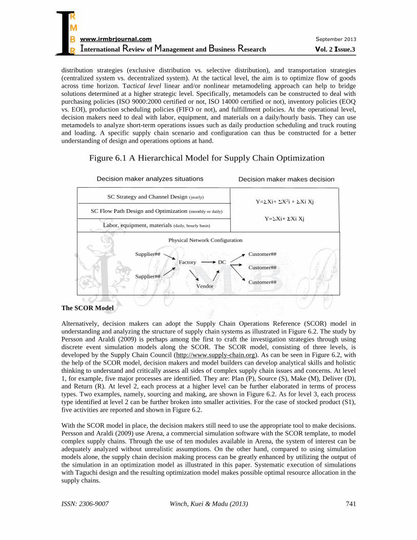
A Hierarchical Model

By drawing on the conceptual model of SCM presented by Simchi-Levi, Kaminsky, and Simchi-Levi

(2000), we report on the possible use of our four-stage problem-solving strategies in dealing with supply

chain issues. Figure 6.1 presents our proposed investigation strategies for a hierarchical model. At the

strategic level, as can be seen in Figure 6.1, company management tends to make high level strategic

choice. Supply chain simulation metamodel can be used in dealing with the selection of number, location,

capacity of supply chain nodes, and the flow of material through the logistics network. The impact of

supply chain quality management (Prado-Prado 2009, Kuei et al. 2008, Kannan & Tan 2007, Fynes, Burca,

& Voss 2005, Robinson & Malhotra 2005), green supply chain management (Kuei, Madu, & Lin 2009,

Preuss 2009, Zhu, Sarkis, Cordeiro, & Lai 2008, Zhu, Sarkis, & Lai 2008), supply chain design initiatives

(Bottani, E. Montanari R. 2009), Collaborative Planning Forecasting and Replenishment programs (Madu &

Kuei 2004), and quick response strategies (Madu & Kuei 2004) can also be evaluated at this strategic level.

Typical examples include reverse logistics strategies (open-loop recycling vs. closed-loop recycling),

I



R M B R



741

distribution strategies (exclusive distribution vs. selective distribution), and transportation strategies

(centralized system vs. decentralized system). At the tactical level, the aim is to optimize flow of goods

across time horizon. Tactical level linear and/or nonlinear metamodeling approach can help to bridge

solutions determined at a higher strategic level. Specifically, metamodels can be constructed to deal with

purchasing policies (ISO 9000:2000 certified or not, ISO 14000 certified or not), inventory policies (EOQ

vs. EOI), production scheduling policies (FIFO or not), and fulfillment policies. At the operational level,

decision makers need to deal with labor, equipment, and materials on a daily/hourly basis. They can use

metamodels to analyze short-term operations issues such as daily production scheduling and truck routing

and loading. A specific supply chain scenario and configuration can thus be constructed for a better

understanding of design and operations options at hand.

Factory DC

Customer##

Customer##

Customer##Vendor

Supplier##

Supplier##

SC Strategy and Channel Design (yearly)

SC Flow Path Design and Optimization (monthly or daily)

Figure 6.1 A Hierarchical Model for Supply Chain Optimization

Physical Network Configuration

Decision maker analyzes situations Decision maker makes decision

Labor, equipment, materials (daily, hourly basis)

Y= Xi+ Xi Xj

Y= Xi+ X2i + Xi Xj

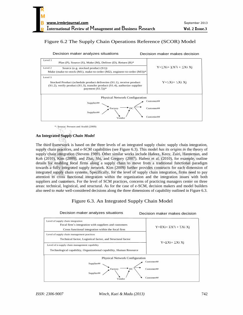
The SCOR Model

Alternatively, decision makers can adopt the Supply Chain Operations Reference (SCOR) model in

understanding and analyzing the structure of supply chain systems as illustrated in Figure 6.2. The study by

Persson and Araldi (2009) is perhaps among the first to craft the investigation strategies through using

discrete event simulation models along the SCOR. The SCOR model, consisting of three levels, is

developed by the Supply Chain Council (http://www.supply-chain.org). As can be seen in Figure 6.2, with

the help of the SCOR model, decision makers and model builders can develop analytical skills and holistic

thinking to understand and critically assess all sides of complex supply chain issues and concerns. At level

1, for example, five major processes are identified. They are: Plan (P), Source (S), Make (M), Deliver (D),

and Return (R). At level 2, each process at a higher level can be further elaborated in terms of process

types. Two examples, namely, sourcing and making, are shown in Figure 6.2. As for level 3, each process

type identified at level 2 can be further broken into smaller activities. For the case of stocked product (S1),

five activities are reported and shown in Figure 6.2.

With the SCOR model in place, the decision makers still need to use the appropriate tool to make decisions.

Persson and Araldi (2009) use Arena, a commercial simulation software with the SCOR template, to model

complex supply chains. Through the use of ten modules available in Arena, the system of interest can be

adequately analyzed without unrealistic assumptions. On the other hand, compared to using simulation

models alone, the supply chain decision making process can be greatly enhanced by utilizing the output of

the simulation in an optimization model as illustrated in this paper. Systematic execution of simulations

with Taguchi design and the resulting optimization model makes possible optimal resource allocation in the

supply chains.

I



R M B R

http://www.supply-chain.org/



742

Factory DC

Customer##

Customer##

Customer##Vendor

Supplier##

Supplier##

Figure 6.2 The Supply Chain Operations Reference (SCOR) Model

Plan (P), Source (S), Make (M), Deliver (D), Return (R)*

Make (make-to-stock (M1), make-to-order (M2), engineer-to-order (M3))*



Y= Xi+ Xi Xj

Y= Xi+ X2i + Xi Xj

Level 1

Level 2

Level 3

Source (e.g. stocked product (S1))

Stocked Product (schedule product deliveries (S1.1), receive product

(S1.2), verify product (S1.3), transfer product (S1.4), authorize supplier

payment (S1.5))*

*: Source: Persson and Araldi (2009)

An Integrated Supply Chain Model

The third framework is based on the three levels of an integrated supply chain: supply chain integration,

supply chain practices, and e-SCM capabilities (see Figure 6.3). This model has its origins in the theory of

supply chain integration (Stevens 1989). Other similar works include Hafeez, Keoy, Zairi, Hanneman, and

Koh (2010), Kim (2009), and Zhai, Shi, and Gregory (2007). Hafeez et al. (2010), for example, outline

details for enabling focal firms along a supply chain to move from a traditional functional paradigm

towards a fully integrated supply network. Kim (2009) further provides constructs for each dimension of

integrated supply chain systems. Specifically, for the level of supply chain integration, firms need to pay

attention to cross functional integration within the organization and the integration issues with both

suppliers and customers. For the level of SCM practices, concerns of practicing managers center on three

areas: technical, logistical, and structural. As for the case of e-SCM, decision makers and model builders

also need to make well-considered decisions along the three dimensions of capability outlined in Figure 6.3.

Figure 6.3. An Integrated Supply Chain Model

Factory DC

Customer##

Customer##

Customer##Vendor

Supplier##

Supplier##

Focal firm’s integration with suppliers and customers

Technical factor, Logistical factor, and Structural factor



Y= Xi+ Xi Xj

Y= Xi+ X2i + Xi Xj

Technological capability, Organizational capability, Human Resource

Cross functional integration within the focal firm

Level of supply chain integration

Level of supply chain management practices

Level of e-supply chain management capability

I



R M B R



743

To begin with, they need to make the process of choice more effective. These issues, however, to the best

of our knowledge, have not been linked with the supply chain simulation metamodels. To answer a “how to

do things better along the three levels of an integrated supply chain” question, it is important to choose the

right decision science tool. Since the simulation metamodeling process illustrated in this paper can involve

several controllable factors and the possible interactions among input variables, adoption of this process

will be helpful in making decisions along an integrated supply chain.

Conclusion

Much has been written about strategizing supply chain systems. Effective supply chain management that

enables a firm to respond to market requirements quickly, reliably, and cost-effectively provides a competitive

advantage. To help develop this advantage, in this paper, we illustrate a four-stage method, involving

experimental designs, regression analyses, validation tests, and decision models, for optimizing supply

chain systems. Three strategic frameworks (see Figures 6.1, 6.2, and 6.3) are also proposed with respect to

the possible use of our metamodeling approaches in dealing with supply chain issues. Our methods and

frameworks will assist in the development of better and effective supply chains at strategic, tactical and

operations levels, and under different organizational conditions.

Potential extensions of the present paper include analyses on the relationships between the effectiveness of

overall supply chain networks and factors such as supply group capacities, reliability of the supply chain stages,

green purchasing policies and promotion tactics. Future research can also include consideration of stages of

growth models and supply chain improvement initiatives such as green supply chain management and the triple

bottom line strategies.

Acknowledgements

This study is partly funded by a grant from the National Science Council, Taiwan, Republic of China

(NSC95-2416-H-006-044-MY2).

References

Bottani, E. & Montanari R. (2009). Supply chain design and cost analysis through simulation. International

Journal of Production Research, 48(10), 1-28.

Chow, W.S., Madu, C.N., Kuei, C., Lu, M.H., Lin, C., & Tseng, H. (2008). Supply chain management in

the US and Taiwan: an empirical study. Omega, 36(5), 665-679.

Chwif, L., Barretto, M.R.P., & Saliby, E. (2002). Supply chain analysis: spreadsheet or simulation?

Proceedings of the 2002 Winter Simulation Conference, 59-66.

Friedman, L.W. & Pressman, I. (1988). The metamodel in simulation analysis: can it be trusted? Journal of

Operations Research Society, 39(10), 939-948.

Fynes. B., Burca. S., & Voss. C. (2005). Supply chain relationship quality, the competitive environment and

performance. International Journal of Production Research, 43(16), 3303-3320.

Hafeez, K., Keoy, K.H.A., Zairi, M., Hanneman, R., & Koh, S.C.L. (2010). E-supply chain operational and

operational and behavioral perspectives: an empirical study of Malaysian SMEs. International Journal of

Production Research, 48(2), 525-546.

Jain, S., Lim, C., Gan, B, & Low, Y. (1999). Criticality of detailed modeling in semiconductor supply chain

simulation. Proceedings of the 1999 Winter Simulation Conference, 888-896.

I



R M B R



744

Kannan, V.R., & Tan, K.C. (2007). The impact of operational quality: a supply chain view. Supply Chain

Management: An International Journal, 12(1), 14-19.

Kelle, P., & Akbulut, A. (2005). The role of ERP tools in supply chain information sharing, cooperation, and

cost optimization. International Journal of Production Economics, 93-94, 41-52.

Kim, S.W. (2009). An investigation on the direct and indirect effect of supply chain integration on firm

performance. International Journal of Production Economics, 119, 328-346.

Kuei, C., Madu, C.N., & Lin, C. (2009). Setting priorities for environmental policies and programs: an

environmental decision making approach. Journal of Design Principles and Practices, 3(5), 315-332.

Kuei, C., Madu, C.N., Lin, C., & Chow, W.S. (2002). Developing supply chain strategies based on the survey

of supply chain quality and technology management. International Journal of Quality & Reliability

Management, 19(7), 889-901.

Kuei, C., Madu, C.N., & Winch, J.K. (2008). Supply chain quality management: a simulation study.

International Journal of Information and Management Sciences, 19(1), 131-151.

Kumar, S., Satsangi, P.S., & Prajapati, D.R. (2013). Optimization of process factors for controlling defects

due to melt shop using Taguchi method. International Journal of Quality and Reliability Management,

30(1), 4-22.

Lee, H.L. (2004). The triple-A supply chain. Harvard Business Review, 82(10), 102-113.

Longo, F. & Mirabelli, G. (2008). An advanced supply chain management tool based on modeling and

simulation. Computers and Industrial Engineering, 54, 570-588.

Madu, C.N., & Kuei, C. (1993). Experimental Statistical Designs and Analysis in Simulation Modeling.

Westport, CT: Quorum.

Madu, C.N., & Kuei, C. (1994). Regression metamodeling in computer simulation – the state of the art.

Simulation Practice and Theory, 2, 27-41.

Madu, C.N., & Kuei, C. (2004). ERP and Supply Chain Management. Fairfield, Connecticut: Chi Publishers.

Maloni, M.J. & Benton, W.C. (1997). Supply chain partnerships: opportunities for operations research.

European Journal of Operational Research, 101, 419-429.

Peace, G.S. (1993). Taguchi Methods. New York, NY: Addison-Wesley.

Persson, F. & Araldi, M. (2009). The development of a dynamic supply chain analysis tool – integration of

SCOR and discrete event simulation. International Journal of Production Economics, 121, 574-583.

Prado-Prado, J. C. (2009). Continuous improvement in the supply chain. Total Quality Management, 20(3),

301-309.

Preuss, L. (2009). Addressing sustainable development through public procurement: the case of local

government. Supply Chain Management: An International Journal, 14(3), 213-223.

Rabelo, L., Eskandari, H., Shaalan, T., and Helal, M. (2007). Value chain analysis using hybrid simulation

and AHP. International Journal of Production Economics, 105, 536-547.

I



R M B R



745

Robinson, C.J. & Malhotra, M.K. (2005). Defining the concept of supply chain quality management and its

relevance to academic and industrial practice. International Journal of Production Economics, 96,

315-337.

Schafer, S. (2005). A Jack Welch of communists. Business Week, May 9, 30-31.

Shang, J.S., Li, S., & Tadikamalla, P. (2004). Operational design of a supply chain using the Taguchi method,

response surface methodology, simulation, and optimization. International Journal of Production

Research, 42(18), 3823-3849.

Shapiro, J.F. (2001). Modeling the Supply Chain. Pacific Grove, CA: Duxbury.

Simchi-Levi, D., Kaminsky, P., & Simchi-Levi, E. (2000). Designing and Managing the Supply Chain.

New York, NY: McGraw-Hill,

Stevens, G.C. (1989). Integrating the supply chain. International Journal of Physical Distribution and

Materials Management, 19(8), 3–8.

Taguchi, C. & Wu, Y. (1980). Introduction to Off-line Quality Control. Nogoya, Japan: Central Japan Quality

Control Association.

Towers, N. & Burnes, B. (2008). A composite framework of supply chain management and enterprise

planning for small and medium-sized manufacturing enterprises. Supply Chain Management: An

International Journal, 13(5), 349-355.

Towill, D.R., Naim, M.M., & Wikner, J. (1992). Industrial dynamics simulation models in the design of supply

chains. International Journal of Physical Distribution and Logistics Management, 22(5), 3-13.

Winch, J. K., Madu, C.N., & Kuei, C. (2012). Metamodeling and optimizing a reverse logistics system.

International Journal of Information and Management Science, 23(1), 41-58.

Zhai, E., Shi, Y., & Gregory, M. (2007). The growth and capability development of electronics

manufacturing service companies. Internal Journal of Production Economics, 107, 1-19.

Zhang, C. & Zhang C.H. (2007). Design and simulation of demand information sharing in a supply chain.

Simulation Modeling Practices and Theory, 15, 32-46.

Zhu, Q., Sarkis, J., Cordeiro, J.J., & Lai, K. (2008). Firm-level correlates of emergent green supply chain

management practices in the Chinese context. Omega, 36, 577-591.

Zhu, Q., Sarkis, J., & Lai, K. (2008). Green supply chain management implications for “closing the loop.”

Transportation Research Part E: Logistics and Transportation Review, 44(1), 1-18.

I



R M B R


constructing multivariate simulation metamodels for supporting supply chain...

Documents