Constructing Decision Trees

A Decision Tree ExampleThe weather data example.

ID code Outlook Temperature Humidity Windy Play

a

b

c

d

e

f

g

h

i

j

k

l

m

n

Sunny

Sunny

Overcast

Rainy

Rainy

Rainy

Overcast

Sunny

Sunny

Rainy

Sunny

Overcast

Overcast

Rainy

Hot

Hot

Hot

Mild

Cool

Cool

Cool

Mild

Cool

Mild

Mild

Mild

Hot

Mild

High

High

High

High

Normal

Normal

Normal

High

Normal

Normal

Normal

High

Normal

High

False

True

False

False

False

True

True

False

False

False

True

True

False

True

No

No

Yes

Yes

Yes

No

Yes

No

Yes

Yes

Yes

Yes

Yes

No

~continuesOutlook

humidity windyyes

no yesyes no

sunny overcast rainy

high normal false true

Decision tree for the weather data.

The Process of Constructing a Decision Tree

• Select an attribute to place at the root of the decision tree and make one branch for every possible value.

• Repeat the process recursively for each branch.

Which Attribute Should Be Placed at a Certain Node

• One common approach is based on the information gained by placing a certain attribute at this node.

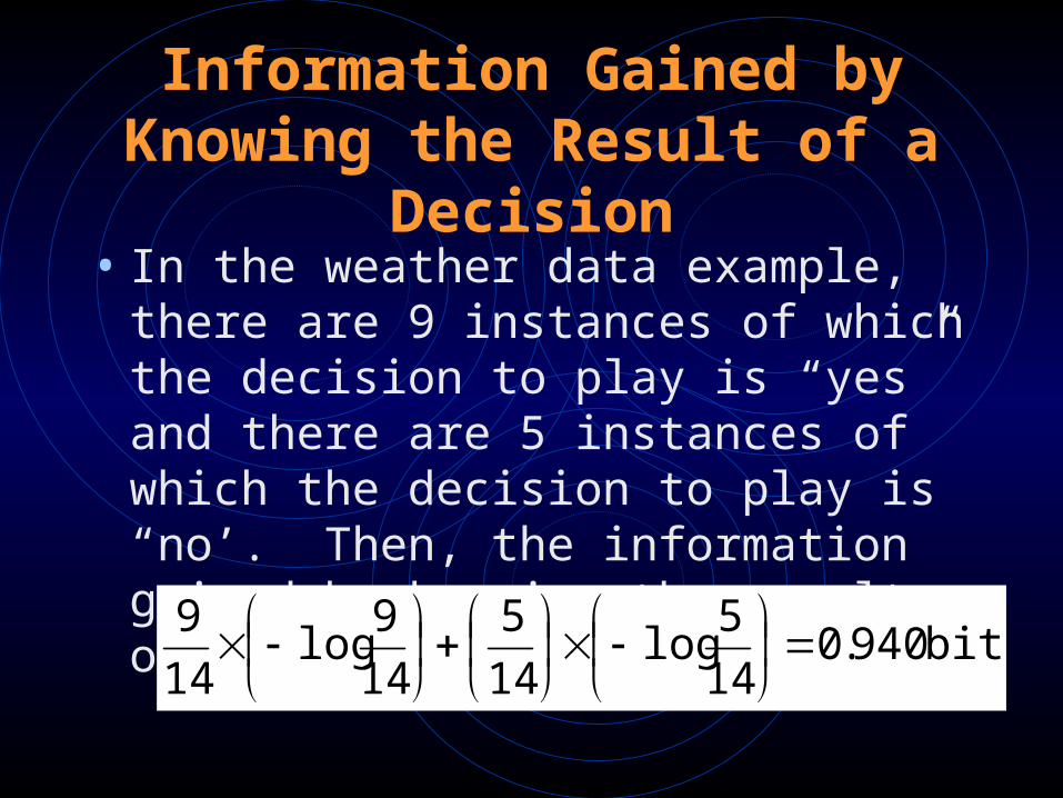
Information Gained by Knowing the Result of a Decision

• In the weather data example, there are 9 instances of which the decision to play is “yes” and there are 5 instances of which the decision to play is “no’. Then, the information gained by knowing the result of the decision is

bits. 940.014

5log

14

5

14

9log

14

9

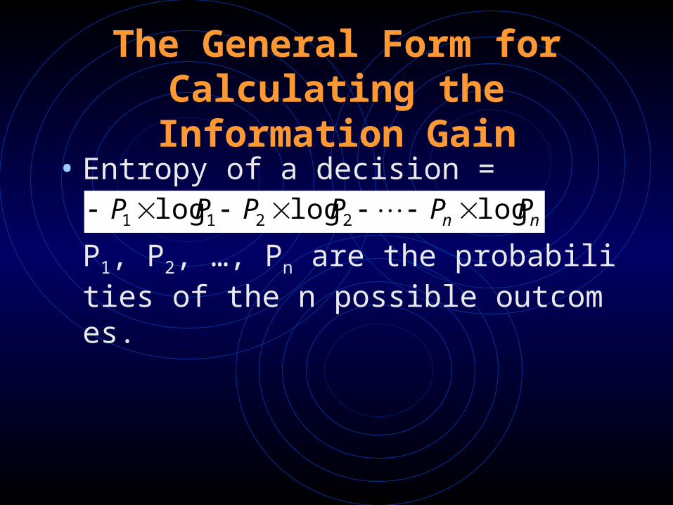
The General Form for Calculating the Information Gain

• Entropy of a decision =

P1, P2, …, Pn are the probabilities of the n possible outcomes.

nn PPPPPP logloglog 2211

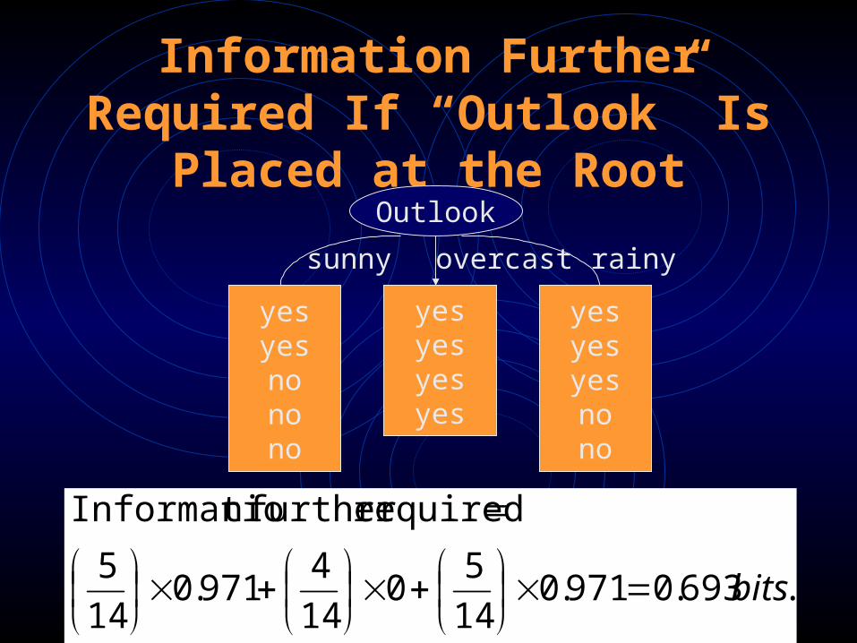
Information Further Required If “Outlook” Is Placed at the Root

Outlook

yesyesnonono

yesyesyesyes

yesyesyesnono

sunny overcast rainy

.693.0971.014

50

14

4971.0

14

5

requiredfurther nInformatio

bits

Information Gained by Placing Each of the 4 Attributes

• Gain(outlook) = 0.940 bits – 0.693 bits

= 0.247 bits.

• Gain(temperature) = 0.029 bits.

• Gain(humidity) = 0.152 bits.

• Gain(windy) = 0.048 bits.

The Strategy for Selecting an Attribute to Place at a Node

• Select the attribute that gives us the largest information gain.

• In this example, it is the attribute “Outlook”.

Outlook

2 “yes” 3 “no”

4 “yes” 3 “yes”2 “no”

sunny overcast rainy

The Recursive Procedure for Constructing a Decision Tree

• The operation discussed above is applied to each branch recursively to construct the decision tree.

• For example, for the branch “Outlook = Sunny”, we evaluate the information gained by applying each of the remaining 3 attributes.• Gain(Outlook=sunny;Temperature) = 0.971 – 0.4 = 0.5

71

• Gain(Outlook=sunny;Humidity) = 0.971 – 0 = 0.971

• Gain(Outlook=sunny;Windy) = 0.971 – 0.951 = 0.02

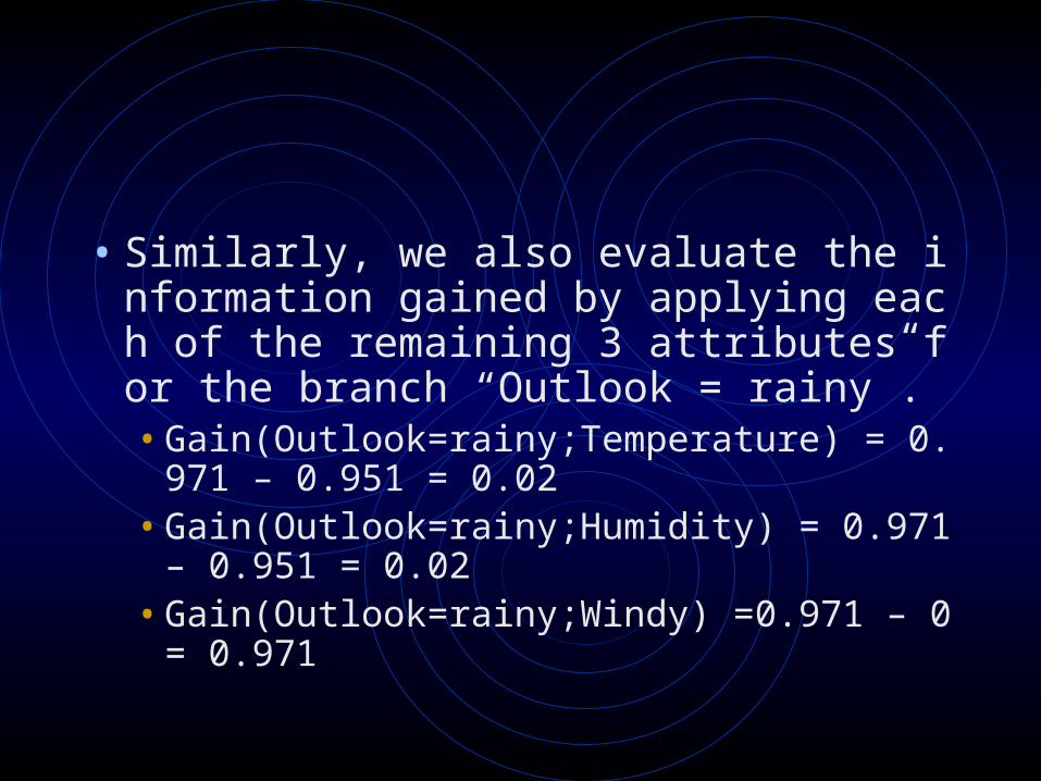
• Similarly, we also evaluate the information gained by applying each of the remaining 3 attributes for the branch “Outlook = rainy”.• Gain(Outlook=rainy;Temperature) = 0.971 – 0.

951 = 0.02• Gain(Outlook=rainy;Humidity) = 0.971 – 0.951

= 0.02• Gain(Outlook=rainy;Windy) =0.971 – 0 = 0.97

1

The Over-fitting Issue

• Over-fitting is caused by creating decision rules that work accurately on the training set based on insufficient quantity of samples.

• As a result, these decision rules may not work well in more general cases.

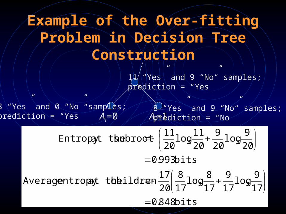
Example of the Over-fitting Problem in Decision Tree Construction

bits 848.0

17

9log

17

9

17

8log

17

8

20

17 children at theentropy Average

bits 993.0

20

9log

20

9

20

11log

20

11 subroot at theEntropy

22

22

11 “Yes” and 9 “No” samples;prediction = “Yes”

8 “Yes” and 9 “No” samples;prediction = “No”

3 “Yes” and 0 “No” samples;prediction = “Yes” Ai=0 Ai=1

• Hence, with the binary split, we gain more information.• However, if we look at the pessimistic error rate, i.e.

the upper bound of the confidence interval of the error rate, we may get different conclusion.

• The formula for the pessimistic error rate is

• Note that the pessimistic error rate is a function of the confidence level used.

user. by the specified level confidence theis and,

samples, ofnumber theis rate,error observed theis where

1

42

1

2

2

222

ccz

nrnz

n

znr

nr

zn

zr

e

• The pessimistic error rates under 95% confidence are

6598.0

17645.1

1

1156706.2

1717

8

1717

8645.1

34645.1

178

4742.0

3645.1

1

36645.1

645.16

645.1

6278.0

20645.1

1

1600706.2

2045.0

2045.0

645.140645.1

45.0

2

22

178

2

22

30

2

22

209

e

e

e

• Therefore, the average pessimistic error rate at the children is

• Since the pessimistic error rate increases with the split, we do not want to keep the children. This practice is called “tree pruning”.

6278.0632.06598.020

174742.0

20

3

Tree Pruning based on 2 Test of Independence

• We construct the corresponding contingency table

Ai=0 Ai=1

Yes 3 8 11

No 0 9 9

3 17 20

11 “Yes” and9 “No” samples;

8 “Yes” and 9 “No” samples;

3 “Yes” and0 “No samples; Ai=0 Ai=1

15.1

20719

20719

-9

2093

2093

-0

201117

201117

-8

20311

20311

-3

statistic The2222

2

• Therefore, we should not split the subroot node, if we require that the 2 statistic must be larger than 2

k,0.05 , where k is the degree of freedom of the corresponding contingency table.

Constructing Decision Trees based on 2 test of Independence

• Using the following example, we can construct a contingency table accordingly.

75 “Yes”s out of100 samples;Prediction = “Yes”

45 “Yes”s out of50 samples;

20 “Yes”s out of 25 samples;

10 “Yes”s out of25 samples; 100

100

50

100

25

100

25100

255155

100

75451020

210

No

Yes

Ai

Ai=0 Ai=1 Ai=2

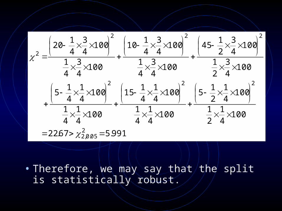
• Therefore, we may say that the split is statistically robust.

991.567.22

10041

21

10041

21

5

10041

41

10041

41

15

10041

41

10041

41

5

10043

21

10043

21

45

10043

41

10043

41

10

10043

41

10043

41

20

205.0,2

222

222

2

Assume that we have another attribute Aj to consider

Aj=0 Aj=1

Yes 25 50 75

No 0 25 25

25 75 100

75 “Yes” out of 100 samples;

50 “Yes” out of 75 samples;

25 “Yes” out of 25 samples; Aj=0 Aj=1

841.311.11

1005752

1005752

-25

1005757

1005757

-50

1002552

1002552

-0

1005752

1005752

-25

205.0,1

2222

2

• Now, both Ai and Aj pass our criterion. How should we make our selection?

• We can make our selection based on the significance levels of the two contingency tables.

.1080008.033.3)1,0(Prob2

33.3)1,0(Prob33.3)1,0(Prob'

11.11)1,0(Prob)11.11(1'11.11

4

22',1 2

1

N

NN

NF

• Therefore, Ai is preferred over Aj.

.1019.111

)67.22(1"67.22

5)67.22(2

1

2",2 2

2

e

F

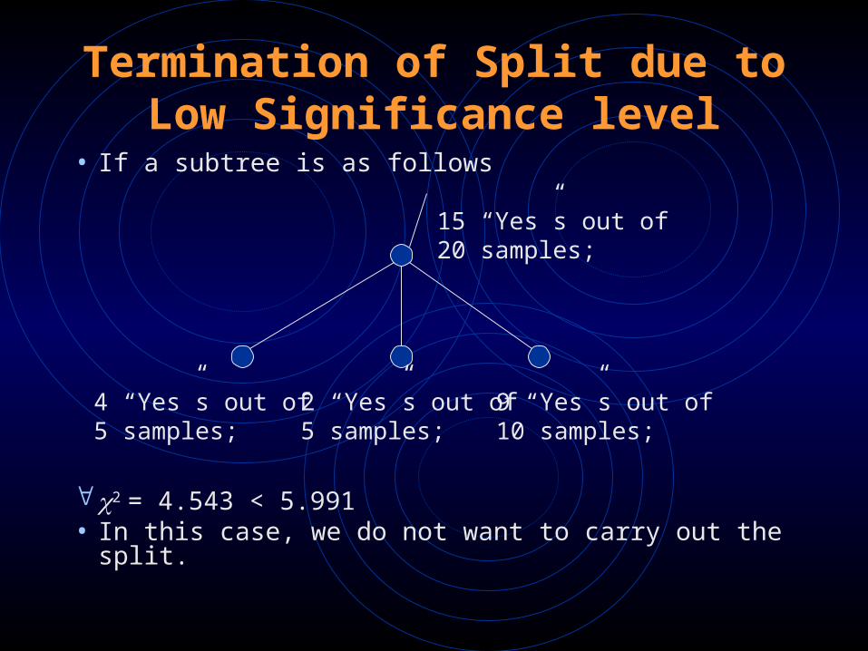
• If a subtree is as follows

2 = 4.543 < 5.991• In this case, we do not want to carry out the split.

15 “Yes”s out of20 samples;

9 “Yes”s out of10 samples;

4 “Yes”s out of 5 samples;

2 “Yes”s out of5 samples;

Termination of Split due to Low Significance level

A More Realistic Example and Some Remarks

• In the following example, a bank wants to derive a credit evaluation tree for future use based on the records of existing customers.

• As the data set shows, it is highly likely that the training data set contains inconsistencies.

• Furthermore, some values may be missing.• Therefore, for most cases, it is impossible to

derive perfect decision trees, i.e. decision trees with 100% accuracy.

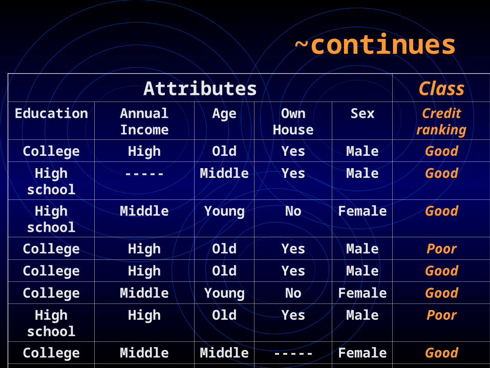
~continues

Attributes ClassEducation Annual Income Age Own House Sex Credit ranking

College High Old Yes Male Good

High school ----- Middle Yes Male Good

High school Middle Young No Female Good

College High Old Yes Male Poor

College High Old Yes Male Good

College Middle Young No Female Good

High school High Old Yes Male Poor

College Middle Middle ----- Female Good

High school Middle Young No Male Poor

~continues

• A quality measure of decision trees can be based on the accuracy. There are alternative measures depending on the nature of applications.

• Overfitting is a problem caused by making the derived decision tree work accurately for the training set. As a result, the decision tree may work less accurately in the real world.

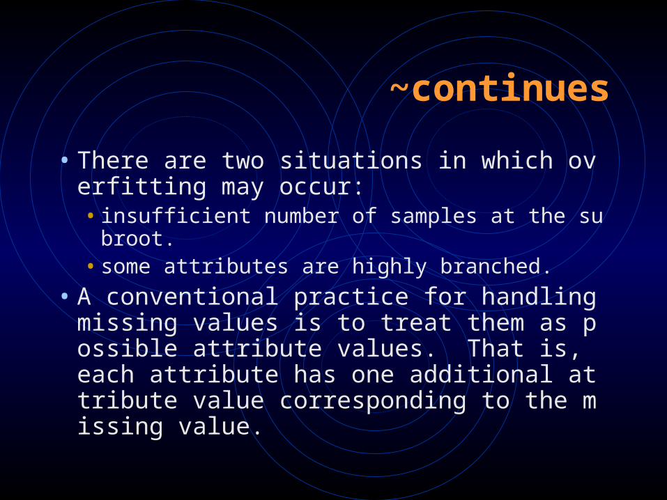
~continues

• There are two situations in which overfitting may occur:• insufficient number of samples at the subroot.• some attributes are highly branched.

• A conventional practice for handling missing values is to treat them as possible attribute values. That is, each attribute has one additional attribute value corresponding to the missing value.

Alternative Measures of Quality of Decision Trees

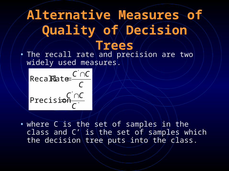
• The recall rate and precision are two widely used measures.

• where C is the set of samples in the class and C’ is the set of samples which the decision tree puts into the class.

' Precision

Rate Recall

C

CC

C

CC

'

'

~continues

• A situation in which the recall rate is the main concern:• “A bank wants to find all the potential credit

card customers”.

• A situation in which precision is the main concern:• “A bank wants to find a decision tree for credit

approval.”