constant ph replica exchange molecular dynamics in

Constant pH Replica Exchange Molecular Dynamics in ExplicitSolvent Using Discrete Protonation States: Implementation, Testing,and ValidationJason M. Swails,† Darrin M. York,‡ and Adrian E. Roitberg*,†

†Quantum Theory Project, Chemistry Department, University of Florida, Gainesville, Florida 32611, United States‡BioMaPS Institute for Quantitative Biology, Center for Integrative Proteomics Research, and Department of Chemistry andChemical Biology, Rutgers University, Piscataway, New Jersey 08901, United States

ABSTRACT: By utilizing Graphics Processing Units, we showthat constant pH molecular dynamics simulations (CpHMD)run in Generalized Born (GB) implicit solvent for long timescales can yield poor pKa predictions as a result of samplingunrealistic conformations. To address this shortcoming, wepresent a method for performing constant pH moleculardynamics simulations (CpHMD) in explicit solvent using adiscrete protonation state model. The method involves standardmolecular dynamics (MD) being propagated in explicit solventfollowed by protonation state changes being attempted in GBimplicit solvent at fixed intervals. Replica exchange along thepH-dimension (pH-REMD) helps to obtain acceptable titrationbehavior with the proposed method. We analyzed the effects of various parameters and settings on the titration behavior ofCpHMD and pH-REMD in explicit solvent, including the size of the simulation unit cell and the length of the relaxationdynamics following protonation state changes. We tested the method with the amino acid model compounds, a smallpentapeptide with two titratable sites, and hen egg white lysozyme (HEWL). The proposed method yields superior predicted pKavalues for HEWL over hundreds of nanoseconds of simulation relative to corresponding predicted values from simulations run inimplicit solvent.

1. INTRODUCTION

Solution pH often has a dramatic impact on biomolecularsystems. By modulating the protonation state equilibria ofvarious, titratable functional groups present in the system, smallchanges in solution pH can affect the charge distribution withinthe biomolecule. This charge distribution, in turn, often has aprofound impact on the fundamental structure and function ofbiomolecules. This effect can be so pronounced that someproteins’ native states are stable only in a narrow pH range,even denaturing completely in extreme pH environments.1,2

Because biomolecular behavior can depend very strongly onthe pH-dependent protonation states of various titratableresidues, accurate computational models designed to treat suchsystems must somehow account for pH effects. While thetraditional approach of assigning a fixed protonation state foreach titratable residue at the beginning of the simulation is stillthe most common approach, numerous methods have beendeveloped in an attempt to treat pH effects in biomoleculesmore quantitatively.3

Of particular interest in this study is the constant pHmolecular dynamics (CpHMD) technique, of which there areseveral variants.4−8 CpHMD is a method that leverages theability of classical molecular dynamics to sample conforma-tional space while simultaneously sampling from the availableprotonation states according to the semigrand canonical

ensemble.5 By adopting this approach, CpHMD simulationscan overcome the limitations imposed by constant-protonationMD simulations by constructing an ensemble whose proto-nation state distributions are properly weighted via thethermodynamic constraint imposed by a constant chemicalpotential of hydronium ions.Within the myriad of available CpHMD methods, there are

two fundamentally different approachescontinuous proto-nation states6,8−11 and discrete protonation states.5,7,12−14 Inthe former, a continuous ‘titration coordinate’ describing afictitious ‘titration particle’ is introduced at each protonable sitethat is propagated as part of the standard MD according to apH-dependent force acting on this particle.6,8 Discreteprotonation state models, on the other hand, employ occasionalMetropolis Monte Carlo (MC) exchange attempts betweendifferent protonation states throughout the course of the MDsimulation.5,7 For the purposes of this study, we will focus onCpHMD models using discrete protonation statesspecificallyas implemented in the AMBER software suite.7

In the original AMBER implementation of CpHMD, themolecular dynamics is propagated treating solvent effectsimplicitly via the Generalized Born (GB) method.7 Periodically

Received: December 2, 2013Published: February 5, 2014

Article

pubs.acs.org/JCTC

© 2014 American Chemical Society 1341 dx.doi.org/10.1021/ct401042b | J. Chem. Theory Comput. 2014, 10, 1341−1352

pubs.acs.org/JCTC

throughout the dynamics, a trial move changing theprotonation state of either one or two closely interactingtitratable residues is evaluated based on the difference inelectrostatic and solvation energies calculated via GB, afterwhich the coordinates are propagated according to this samepotential.Recently, however, Machuqueiro and Baptista raised

concerns about pKa predictions inheriting problems related tothe model compound definition and inaccuracies in theunderlying force field.15 In particular, force field deficiencieshave been shown to result in incorrecteven unphysicalglobal minima.16−20 So far, reported applications of Mongan etal.’s method have shown good results because the simulationswere too short to reveal the full extent of the weaknesses in theGeneralized Born model being used.7,12,21−24 When weimplemented Mongan et al.’s method on graphics processingunits (GPUs) in order to run long simulations, the unphysicalstates sampled over long time scales degraded the pKapredictions of the hen egg-white lysozyme (HEWL). Thiserroneous sampling may be addressed to some extent by usingan explicit representation of the solvent to propagate thedynamics.While most of the physics-based methods designed to

describe a biomolecular system at constant pH use an implicitsolvent representation of the solvent, several CpHMD methodshave been extended to sample, at least conformations, inexplicit solvent with both the discrete5 and continuous9−11

protonation models. The methods proposed by Baptista et al.5

and Wallace and Shen9 use an implicit solvent potential tosample protonation states while the methods developed by Gohet al.10 and Donnini et al.11 perform λ-dynamics on the titrationcoordinate directly in explicit solvent. A more recent approachby Wallace and Shen uses a λ-dynamics approach in pureexplicit solvent and adds a counterion whose charge is changedsimultaneously with a titratable residue in order to maintaincharge neutrality in the unit cell.25

Discrete protonation methods use molecular dynamics topropagate the spatial coordinates, while occasionally interrupt-ing the dynamics to attempt changes to the protonation statesof the titratable residues using a Metropolis Monte Carlocriteria. The CpHMD method implemented in AMBER7 (andlater implemented in CHARMM12) performs MD in GBsolvent, periodically attempting to change the protonation stateof one or two interacting residues roughly every 10 fs.7 In thestochastic titration method described by Baptista et al.,dynamics is run in explicit solvent for 2 ps,26 after which acycle of protonation state change attempts are evaluated usingthe Poisson−Boltzmann (PB) equation to treat solvationeffects for every titratable residue and interacting titratableresidue pair. About 40 000 full cycles are attempted each timeprotonation state changes are attempted.27 Afterward, thesolute is held fixed while MD is propagated on the solvent toreorganize the solvent distribution to the new set ofprotonation states.Implicit solvent modelsin this case GB and PBaverage

over all solvent degrees of freedom, thereby instantlyincorporating the effects of solvent relaxation around discreteprotonation state changes. Therefore, MC moves in which aprotonation state change is attempted have a reasonableprobability of succeeding when the solution pH is set close tothe pKa of the titratable group. When explicit solvent moleculesare present, however, the solvent orientation around anysolvent-exposed, titratable residue will oppose any protonation

state changes. On average, the solvent distribution tends toresist protonation state changes by imposing a barrier on theorder of 100 kcal/mol as estimated by measurements in our laband in others’,9 making titration with discrete protonationstates difficult directly in explicit solvent.In this study, we present a new method of performing

CpHMD simulations in explicit solvent using discreteprotonation states. This method is similar in some regards tothat used by Baptista et al.,5 and we evaluate its performance onthe model compounds, a pentapeptide, and the HEWL protein.To enhance the sampling capabilities of this new CpHMDmethod, we use replica exchange in the pH-dimension (pH-REMD), whose theory and performance were discussedpreviously in the context of implicit solvent calculations.12,24

This paper is organized as follows: We will first describe themethod and its implementation in the Theory and Methodssection, followed by a description of the calculations weperformed in the Calculation Details section. Afterward, we willevaluate its performance as well as sensitivity to the method’stunable parameters in the Results and Discussion section.

2. THEORY AND METHODSIn this section, we will discuss the details of our proposedmethod and highlight how it differs from the approach used byBaptista et al.5 The theoretical foundation of our CpHMDmethod is described in detail, as well as the pH-REMD methodwe used in our simulations.

2.1. Conformational and Protonation State Sampling.In CpHMD, structures are sampled from the semigrandcanonical ensemble, whose probability distribution function isgiven by

∫ρ

βμ ββμ β

=* −

∑ ′ ′ * ′ − ′ ′ ′′

n Hd d n H

q p nq p n

p q p q n( , , )

exp( ( , , ))

exp( ( , , ))n(1)

where β = 1/kBT, μ* is the chemical potential of hydronium(directly related to the solution pH), q is the generalizedcoordinates of the system particles, p is the conjugatemomenta, and n is the total number of titratable protonspresent in that state. When bold, n refers to the protonationstate vector, specifying not only the total number of protonspresent but on which titratable sites those protons are located.The denominator in eq 1 is the partition function of thesemigrand canonical ensemble.To sample from the probability function ρ in eq 1, discrete

protonation state methods use MD with a fixed set ofprotonation states to sample coordinates and momenta coupledwith a MC-based protonation state sampling at fixedconformations throughout the trajectory. Baptista et al. showedthat standard MD, which samples ρ(q,p|n), used in conjunctionwith MC moves on protonation states, which samples fromρ(n|q,p), properly samples from the desired probabilitydistribution function ρ(q, p, n).5 In this notation, ρ(q,p|n) isthe conditional probability function of the positions andmomenta with fixed protonation states whereas ρ(n|q,p) is theconditional probability function of the protonation state vectorat a fixed protein conformation.In explicit solvent, ρ(n|q,p) is difficult to sample directly,

since the solvent orientation is relaxed with respect to thecurrent protonation state vector. Following the arguments ofBaptista et al., the system coordinates (and momenta) can beseparated into solute and solvent degrees of freedom.5 The

Journal of Chemical Theory and Computation Article

dx.doi.org/10.1021/ct401042b | J. Chem. Theory Comput. 2014, 10, 1341−13521342

protonation state sampling is then performed according to theconditional probability

ρ ρ′ = |′ ′ ′p q n p q( )solvent solvent solute solute (2)

where qsolvent and psolvent are relaxed solvent distributions ofpositions and momenta around the protonation state vector, n.5

The energy differences resulting from the relaxed solventdistributions around the different protonation states arequantities that implicit solvent models strive to reproduce.Therefore, the distribution function ρ′ in eq 2 can beapproximated using continuum models, such as the PB orGB equations, thereby avoiding the otherwise costly solventrelaxation calculation associated with each attempted proto-nation state change. Performing relaxation MD on the solventdegrees of freedom should be done after protonation statechanges to generate the uncorrelated, relaxed solventdistribution required by eq 2. While using MD to generaterelaxed solvent distributions violates detailed balancemicro-scopic reversibility is no longer preservedManousiouthakisand Deem have shown that simply satisfying the weaker balancecondition is valid.28

Contrary to the stochastic titration method that calculatedsolvation free energies using the PB equation to evaluateprotonation state changes,5 we chose to use the GB implicitsolvent model for three main reasons. First, AMBER hasnumerous GB models readily available,29−33 allowing us to usethe existing code to evaluate protonation state change attempts.Second, results from the original GB-based CpHMDimplementation by Mongan et al., and from a number ofprevious studies using the method, have been promis-ing.7,22,24,34 Furthermore, GB was shown to be effective whenused in a hybrid solvent method with continuous protonationstates,9 is computationally cheaper than PB, and GB is moreeasily parallelizable, allowing longer simulations to beperformed in the same amount of time.2.2. Explicit Solvent CpHMD Workflow. The process of

the CpHMD method presented here can be divided into threerepeating steps, summarized in the workflow diagram in Figure1. This workflow is very similar to the one presented in ref 5(Figure 2), although the nature of the MC protonation statemove is different.In the proposed method standard MD in explicit solvent is

carried out using a constant set of protonation states (an initialset must be provided at the start of the simulation). At somepoint the MD is stopped, the solvent (including anynonstructural ions) are stripped, the potential is switched toan available GB model, and a set of N protonation state changesare attempted where N is the number of titratable residues.While in principle the MD can be stopped randomly with apredetermined probability at any step, in this iteration of ourproposed method we run MD for a set time interval, τMD,similar to the stochastic titration method.5

After the MD is halted and the solvent stripped, protonationstate changes are proposed for each titratable residue once, inrandom order, choosing from the available protonation states ofthat residue excluding the currently occupied state. Theelectrostatic energy difference between the proposed andcurrent protonation states, as well as the MC decision regardingwhether or not to accept the proposed state, are calculated thesame way as in the original GB implementation.7 If theprotonation state change is accepted, the ‘current’ state isappropriately updated, and the next residue, chosen at randomwithout replacement, is titrated with this new state.

For each residue that is titrated, there is a 25% chance that aso-called multisite titration will occur with a neighboringresidue; that is, the proposed change will involve changes to theprotonation state of both the residue and its neighbor. Twotitratable residues are considered ‘neighbors’ if any two titratinghydrogen atoms are within 2 Å from each other. If eitherresidue has more than one titrating proton, the two residues areneighbors if the minimum distance between any pair of titratinghydrogens meets the cutoff.Including multisite protonation state jumps is important for

systems that have closely interacting titratable residues.Without these multisite moves, proton transfers betweenadjacent titratable residues involved in a hydrogen bondwould never occur due to the high penalty of disrupting theinteraction by adding another proton or removing the protoninvolved in the hydrogen bond. This feature was actuallypresent in the initial GB CpHMD implementation, and whileno mention of it was made in the original paper, a small notewas made in the AMBER Users’ manual.7

If any of the protonation state change attempts wereaccepted, the solute is frozen while MD is performed on thesolvent (and any ions) to relax the solvent distribution aroundthe new protonation states. The length of this relaxation is atunable parameter of the method, which we will call τrlx. Afterthe relaxation is complete, the velocities of the solute atoms arerestored to their values prior to the relaxation and the standarddynamics is continued.It is worth noting that as the protonation states change

during the course of the CpHMD simulations, so too does thenet charge on the system. Because we are using periodic

Figure 1. Workflow of the proposed discrete protonation CpHMDmethod in explicit solvent. Following the standard MD, the solvent,including all nonstructural ions (as determined by user-input), arestripped and the protonation state changes are evaluated in a GBpotential. After that, the solvent and the original settings are restoredfor the remaining steps.



boundary conditions with a lattice-sum method to computeelectrostatics, finite-size effects involving the changing chargesare introduced.35,36 The investigations focusing on charge-dependent finite-size effects have identified artifacts affectingprimarily computed free energies and pressure and are largerfor smaller unit cells.35 In the proposed method, theprotonation state changes are attempted in implicit solventwith a GB potential, which is entirely unaffected by these finite-size effects. Furthermore, since replica exchange simulations inAMBER require the use of constant volume, no pressurecorrections are required, either.2.3. pH-based Replica Exchange. The underlying theory

behind replica exchange in pH-space with MD run in explicitsolvent is unchanged from the version we implemented inimplicit solvent earlier.12,24 Replicas are ordered by theirsolution pH parameter, and adjacent replicas attempt toexchange their pH periodically throughout the MD simulations.The probability of accepting these replica exchange attempts,

given by eq 3, depends only on the difference in the number oftitrating protons present in each replica and their respectivedifference in pH.24

= − −→P N Nmin{1, exp[ln 10( )(pH pH )]}i j i j i j (3)

where Ni is the total number of titratable protons ‘present’ instate i.Because the probability of accepting replica exchange

attempts depends only on the number of titratable protonsthat are present in the system, the number of replicas necessaryto obtain efficient mixing in pH-space does not increase asexplicit solvent is added. This, coupled with the more accuratesampling found with explicit solvent simulations,24 makes pH-REMD an effective tool for explicit solvent CpHMD.

3. CALCULATION DETAILS

To evaluate the performance of the proposed method, weapplied it to the amino acid model compounds, a smallpentapeptide (ACFCA), and a protein commonly used in pKacalculation studies-the hen egg-white lysozyme (HEWL).3.1. Implicit Solvent Simulations. In order to allow

simulations to be run for hundreds of nanoseconds, weimplemented Mongan et al.’s CpHMD method with pH-REMD24 on GPUs in GB implicit solvent.37 We used theHEWL structure solved in PDB code 1AKI38 as our startingstructure. The carboxylate residues were initially set in thedeprotonated state, and histidine 15 was started in the double-protonated state according to AMBER defaults.The structure was minimized using 10 steps of the steepest

descent algorithm followed by 990 steps of conjugate gradientwith 10 kcal/mol·Å2 . The minimized structure was then heatedfor 1 ns, varying the target temperature linearly from 10 to 300K over 667 ps. Positional restraints (5 kcal/mol·Å2) wereplaced on the backbone atoms. The temperature was controlledusing Langevin dynamics with a 5 ps−1 friction coefficient.The heated structure was then equilibrated at 300 K for 2 ns

using Langevin dynamics with a friction coefficient of 10 ps−1

with 0.1 kcal/mol·Å−2 positional restraints on the backbone.We then ran 500 ns of pH-REMD, attempting to changeprotonation states every 10 fs and attempting replica exchangesevery 20 fs. We used 14 replicas spanning the pH range 1−7.5with a 0.5 pH-unit spacing between adjacent replicas. Nononbonded cutoff was used for any implicit solvent simulation.

3.2. Model Compounds. Absolute pKa values are verydifficult to calculate in solution; they are impossible usingclassical force fields. As a result, every physics-based CpHMDmethod uses the idea of a model compound whose experimentalpKa is easy to measure with a high level of accuracy. Anempirical parameterthe reference energyis then added sothat CpHMD reproduces the experimental pKa values of thesecompounds. The reference energy must be set for the solvationmodel that is used during the simulations, which was the sameGBOBC model that Mongan et al. used in their study.7

The model compounds have the residue sequence ACE-X-NME, where ACE is a neutral acetyl capping residue, X is thetitratable residue, and NME is a neutral methyl amine cappingresidue.7 The available titratable residues in AMBER areaspartate (AS4), glutamate (GL4), histidine (HIP), lysine(LYS), tyrosine (TYR), and cysteine (CYS), which are alldefined as described by Mongan et al.7 A 10 Å TIP3P39 solventbuffer was added in a truncated octahedron around each modelcompound that we simulated. The aspartate model compoundwas also simulated with larger box sizes15 Å and 20 Åbuffersto determine if it had any effect on the calculated pKa.After the system topologies were generated, each system was

minimized using 100 steps of steepest-descent minimizationfollowed by 900 steps of conjugate gradient minimization. Theywere then heated at constant pressure, varying the targettemperature linearly from 50 to 300 K over 200 ps. Thesolvated model compounds were then run for 2 ns at constanttemperature and pressure.Each model compound system was simulated at constant pH

and volume for 2 ns, setting τrlx = 200fs. Each simulationemployed pH-REMD using six replicas with the solution pH setto pKa ± 0.1, pKa ± 0.2, and pKa ± 1.2. To evaluate the effect ofthe solvent relaxation time, the cysteine model compound wasrun with τrlx set to 10 fs, 40 fs, 100 fs, 200 fs, and 2 ps.

3.3. ACFCA. A pentapeptide with the sequence Ala-Cys-Phe-Cys-Ala (ACFCA) was solvated with a 15 Å buffer of TIP3Pmolecules around the solute in a truncated octahedron.The system was minimized using 100 steps of steepest

descent minimization followed by 900 steps of conjugategradient. The minimized structure was heated by varying thetarget temperature linearly from 50 to 300 K over 200 ps atconstant pressure. The resulting structure was then simulated at300 K at constant temperature and pressure to stabilize thesystem density and equilibrate the solvent distribution aroundthe small peptide.The resulting structure was then used in simulations at six

different solution pH values7.1, 8.1, 8.3, 8.7, 8.9, and 9.9.These pH values were chosen because the pKa of the cysteinemodel compound is 8.5, so the two cysteines of ACFCA wereexpected to titrate in this pH range. To demonstrate the effectthat pH-REMD had on the titration of ACFCA, two sets ofsimulations were runCpHMD with no exchanges and pH-REMDwith each replica being run for 2 ns.

3.4. Hen Egg White Lysozyme. We used the structuresolved in PDB code 3LZT as the starting structure for oursimulations.40 All eight aspartate residues were renamed AS4,both glutamate residues were renamed GL4, and histidine 15was renamed HIP in preparation for the pH-REMDsimulations.All disulfide bonds were added manually in tleap, and the

system was solvated with a 10 Å TIP3P water buffersurrounding the protein in a truncated octahedron. We added26 sodium ions and 11 chloride ions in random locations in the



simulation cell to provide an ionic atmosphere and neutralizethe system in its initial, default protonation states.The system was minimized using 1000 steps of steepest

descent minimization followed by 4000 steps of conjugategradient, with 10 kcal/mol·Å2 positional restraints applied tothe backbone. The structures were then heated at constantvolume, varying the target temperature linearly from 10 to 300K over 400 ps using Langevin dynamics with a 5 ps−1 frictioncoefficient. The heated structures were then equilibrated for 4ns at constant temperature and pressure using Langevindynamics with a 2 ps−1 friction coefficient to maintain thetemperature and 2 ps−1 coupling constant for the Berendsenbarostat. The system was then subjected to 112 ns ofequilibration MD at constant volume and temperature usingLangevin dynamics with a 2 ps−1 friction coefficient to maintaina constant temperature of 300 K.Following the setup stages of the simulations, two sets of pH-

REMD simulations were carried out for 122 and 150 ns with 12replicas spanning the pH range from −3 to 8 at 1 pH-unitintervals to characterize the acidic-range titration behavior ofHEWL.3.5. Simulation Details. All systems were parametrized

using the AMBER FF10 force field, which is equivalent to theAMBER FF99SB force field for proteins.19 The tleap programof the AmberTools 12 program suite was used to build themodel compound and ACFCA molecules, to add hydrogenatoms HEWL and to solvate each system that was run inexplicit solvent.All simulations were performed using either the sander or

pmemd module of a development version of AMBER 12.41

Langevin dynamics was used in every simulation to maintainconstant temperature with collision frequencies varying from 1ps−1 to 5 ps−1, and the random seed was set from the computerclock to avoid synchronization artifacts.42,43 The Berendsenbarostat was used to maintain constant pressure for theequilibration dynamics with a coupling constant of 1 ps−1.All molecular dynamics, including the solvent relaxation

dynamics, are run with a 2 fs time step, constraining bondscontaining hydrogen using SHAKE.44,45 Replica exchange

attempts between adjacent replicas were made every 200 fsfor all pH-REMD simulations. Protonation state changes wereattempted every 200 fs for all constant pH simulations.Long-range electrostatic interactions were treated with the

particle-mesh Ewald method46,47 using a direct-space and vander Waals cutoff of 8 Å. Defaults were used for the remainingEwald parameters. The GB model proposed by Onufriev et al.,indicated by the parameter igb = 2 in sander,31 was used toevaluate the protonation state change attempts to be consistentwith the original implementation in implicit solvent.7 Theintrinsic solvent radius of the carboxylate oxygen atoms wasreduced from the standard value of 1.5 Å to 1.3 Å tocompensate for the effect of having 2 dummy protons presenton each oxygen in the syn- and anti-positions in the explicitsolvent simulations.7

The deprotonation fraction ( fd) and pH for eachsimulationand each window of the running averageswasfitted to the Hill equation (eq 4) using the Levenberg−Marquardt nonlinear least-squares algorithm implemented inSciPy to compute the pKa and Hill coefficient (n). All pKavalues reported for titratable residues in this paper correspondto the value computed by fitting fd from the simulations at everypH to eq 4 over the specified time interval.

=+ −f

11 10n Kd (p pH)a (4)

4. RESULTS AND DISCUSSION

First, we will analyze the long simulations in implicit solventthat demonstrate the weaknesses of implicit solvent models.Next, we will analyze our proposed CpHMD and pH-REMDmethods as well as ways to optimize its overall performance.We will start by discussing the behavior of the modelcompounds when the size of the unit cell and the length ofthe relaxation dynamics (τrlx) is varied. We will follow thisdiscussion with a similar analysis on a slightly larger systemACFCAbefore discussing the application of our proposedmethod to HEWL.

Figure 2. RMSD compared to the 1AKI crystal structure for the ensembles at pH 1, 4, and 7. The time series is shown on the left with thenormalized histograms shown on the right.



4.1. Long GB Simulations. Long simulations are requiredto observe rare events or phenomena that occur on long timescales, but often expose deficiencies in a computational modelthat are frequently missed in shorter simulations.48 Therefore,we ran CpHMD GB simulations of HEWL for 600 nsmorethan an order of magnitude longer than what has previouslybeen publishedto determine if these calculations were stableand could be used to study the dynamical behavior of proteinsover long time scales.The backbone RMSD with respect to the starting crystal

structure, shown in Figure 2 for the replicas at pH 1, 4, and 7,reaches as much as 10 Å at lower pH values, suggesting that thenative state is unstable in GB implicit solvent at long timescales. As the lysozyme is active at the lysosomal pH around4.5, CpHMD simulations near this pH should reflect thisstability. As the backbone RMSD from the crystal structureincreases, the predicted pKa value worsens. We computed theroot mean squared error (RMSE) of the computed acidicresidue pKa values compared to experiment. The predicted pKawas computed for each residue by taking a running averagewith a 10 ns window of the deprotonation fraction for eachresidue at each pH in the pH-REMD simulation. The RMSE ofthe calculated pKa values from experiment averaged over alltitratable residues is shown in Figure 3.

4.2. Explicit Solvent Simulations. 4.2.1. Box Size Effects.To study the effect that the unit cell size has on titrations in ourproposed method, we prepared three simulations of theaspartate model compound with different TIP3P solventbuffers surrounding it. We prepared systems with a 10 Å, 15Å, and 20 Å TIP3P solvent buffer around the model aspartate.Because protonation state sampling takes place in GB solvent

without periodic boundary conditions, any effect of the box sizeon calculated pKa values can only arise due to alterations of the

structural ensembles induced by artifacts from the box size. Thecalculated pKa values of the three systems were 4.02 ± 0.07,4.05 ± 0.08, and 4.12 ± 0.07 for the 10 Å, 15 Å, and 20 Åsolvent buffer systems, respectively. To estimate the un-certainties we divided each simulation into 100 ps chunksand took the standard deviation of the set of 20 pKa valuescalculated from those segments.To further demonstrate the insensitivity of box size to pH-

REMD titrations, we plotted the solvent radial distributionfunctions (RDFs) around the center of mass of the carboxylatefunctional group in Figure 4. The insensitivity of the pKa andsolvent structure with respect to the model compound providesstrong evidence that no undue care is necessary when choosingthe size of the solvent buffer for these types of simulations.

4.2.2. Effect of Solvent Relaxation Time (τrlx). An importantapproximation in the proposed method is that the protonationstate sampling ρ′ from eq 2 can be replaced using an implicitsolvent model followed by relaxation MD to generate therelaxed solvent positions and momenta. The question thenbecomes how long this relaxation dynamics should be run.To address this, 2 ns of constant protonation molecular

dynamics simulations were run on the model cysteinecompound in both protonation statesprotonated anddeprotonatedafter the same minimization and heatingprotocols were used as for the other model compoundsimulations. The protonation state was then swapped for thefinal structures of both simulations, and MD was performedwhile constraining the solute position for 20 ns, equivalent tothe relaxation dynamics protocol in our proposed method.The optimum value for τrlx is the time after which the energy

of the relaxation trajectory stabilizes and the simulation loses allmemory of its initial configuration. To be truly equivalent tohaving been chosen at random, the final, relaxed solventdistribution must be completely uncorrelated from the initialdistribution at the time the protonation state was changed.To probe the necessary time scales for these relaxation

dynamics, the energy of each snapshot in the relaxationtrajectory is plotted alongside the autocorrelation function ofthat energy in Figure 5 to clearly demonstrate the ‘appropriate’value of τrlx for this model system.We chose the cysteine model compound for this test for two

reasons. First, the model compounds are fully solvent-exposeddue to their small size, which results in a worst-case scenario interms of the number of water molecules that must bereorganized during the relaxation dynamics. The optimum τrlxvalue for model compounds is expected to be an upper-boundon the values required for larger systems. Second, cysteine isthe smallest and simplest of the titratable amino acids,eliminating potential complications from tautomeric statescompared to aspartate, glutamate, and histidine.The relaxation energies plotted in Figure 5 begin to stabilize

after 4 to 6 ps of relaxation dynamics and are largelyuncorrelated within that same time scale. However, because 4ps of MDcorresponding to 2000 steps of dynamics with a 2fs time stepadds dramatically to the cost of CpHMDsimulations in explicit solvent, we will analyze the approx-imation of using a significantly smaller value for τrlx.Both the relaxation energies and autocorrelations drop very

sharply at the start of the relaxation dynamics, so the majorityof the benefit gained by relaxing the solvent is realized withinthe first few steps.For both simulations, the first 200 fs of relaxation dynamics

resulted in 70% of the total relaxation energy in calculations.

Figure 3. RMSE of all acidic titratable residue pKa values compared toexperiment49 during the course of the simulation. A 10 ns window wasused for the running average of the computed pKa.



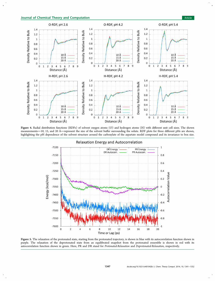
Figure 4. Radial distribution functions (RDFs) of solvent oxygen atoms (O) and hydrogen atoms (H) with different unit cell sizes. The shownmeasurements10, 15, and 20 Årepresent the size of the solvent buffer surrounding the solute. RDF plots for three different pHs are shown,highlighting the pH dependence of the solvent structure around the carboxylate of the aspartate model compound and its invariance to box size.

Figure 5. The relaxation of the protonated state, starting from the protonated trajectory, is shown in blue with its autocorrelation function shown inpurple. The relaxation of the deprotonated state from an equilibrated snapshot from the protonated ensemble is shown in red with itsautocorrelation function shown in green. Here, PR and DR stand for Protonated-Relaxation and Deprotonated-Relaxation, respectively.



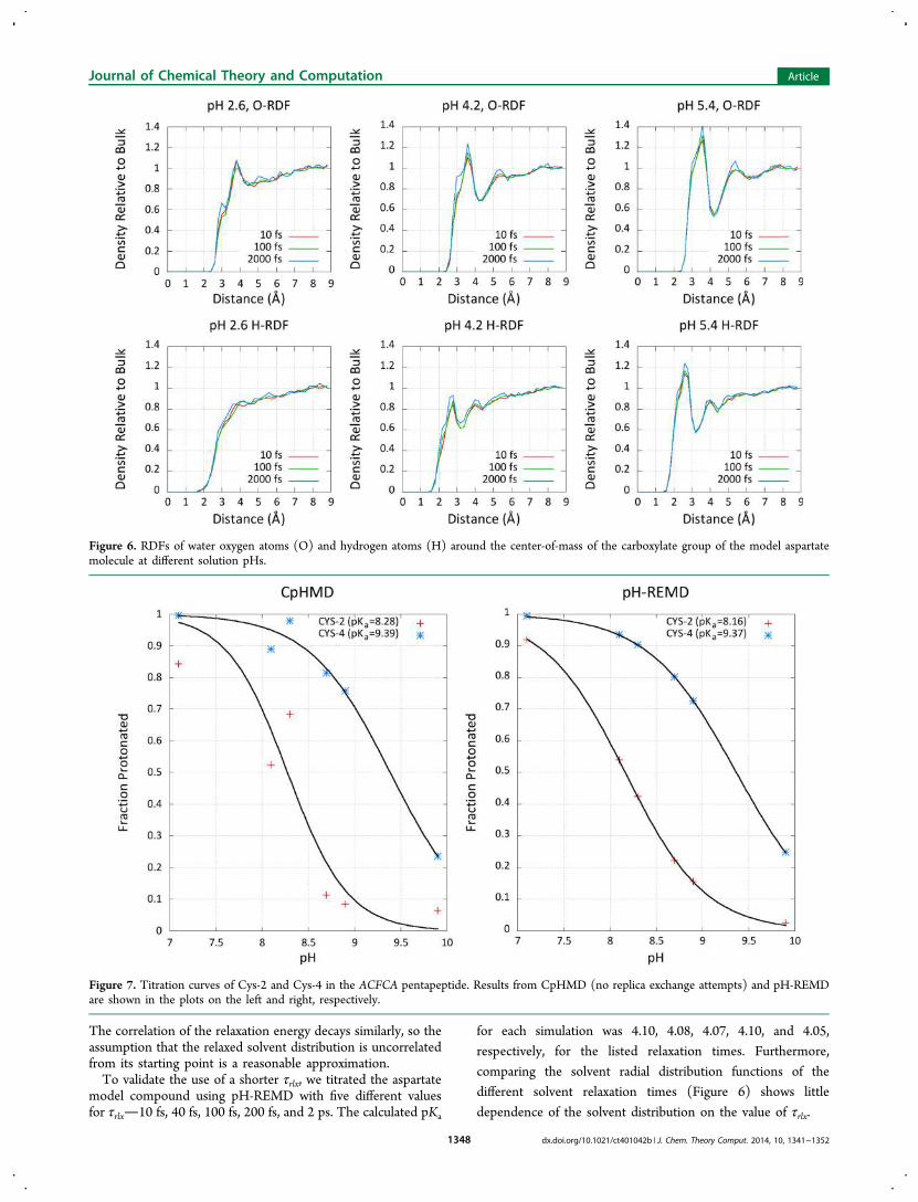
The correlation of the relaxation energy decays similarly, so theassumption that the relaxed solvent distribution is uncorrelatedfrom its starting point is a reasonable approximation.To validate the use of a shorter τrlx, we titrated the aspartate

model compound using pH-REMD with five different valuesfor τrlx10 fs, 40 fs, 100 fs, 200 fs, and 2 ps. The calculated pKa

for each simulation was 4.10, 4.08, 4.07, 4.10, and 4.05,respectively, for the listed relaxation times. Furthermore,

comparing the solvent radial distribution functions of thedifferent solvent relaxation times (Figure 6) shows little

dependence of the solvent distribution on the value of τrlx.

Figure 6. RDFs of water oxygen atoms (O) and hydrogen atoms (H) around the center-of-mass of the carboxylate group of the model aspartatemolecule at different solution pHs.

Figure 7. Titration curves of Cys-2 and Cys-4 in the ACFCA pentapeptide. Results from CpHMD (no replica exchange attempts) and pH-REMDare shown in the plots on the left and right, respectively.



4.2.3. ACFCA: CpHMD vs pH-REMD. The small peptidechain ACFCA, described in section 3.3, was chosen as a testdue to its small size and predictable titration behavior. Thesimplicity of the system makes it an ideal test; its small sizemitigates the conformational sampling problem, and the simpletitrating behavior of cysteine further simplifies protonation statesampling. Unlike aspartate and glutamate, which have the fourdefined tautomeric states defined by anti- and syn-protonationon each of two carboxylate oxygens, and histidine which hastwo tautomeric states on the imidazole, cysteine has only oneprotonated and one deprotonated state, presenting fewerdegrees of freedom that must be exhaustively sampled.Each cysteine is in a slightly different microenvironment due

to the different charges of the N- and C-termini. Due to itsproximity to the N-terminus, Cys-2 is expected to experience anegative pKa shift with respect to the model compound due tothe electrostatic interactions with the positively chargedterminus. Cys-4, on the other hand, is expected to experiencea pKa shift in the opposite direction due to the electrostaticinteractions with the negatively charged C-terminus.We ran simulations at pH 7.1, 8.1, 8.3, 8.7, 8.9, and 9.9 to

sufficiently characterize the titration behavior of both cysteineresidues around their pKa values. One set of replicas was runwith pH-REMD while the other set was run using CpHMD(i.e., without attempting exchanges between the replicas). Thetitration curves for both sets of simulations, shown in Figure 7,demonstrate the importance of using pH-REMD in constantpH simulations in explicit solvent. As expected, the pH-REMDsimulations revealed pKa shifts of −0.2 pK units for Cys 2 and+0.9 pK units for Cys 4 with respect to the model Cyscompound.Even for a simple system such as ACFCA, using pH-REMD

on top of standard CpHMD simulations results in a drasticimprovement in titration curve fita result of improvedprotonation state sampling. The residual sum of squares (RSS),a quantity that measures how well an equation fits a data set,shows drastic improvement using pH-REMD. The RSS forCys-2 and Cys-4 using CpHMD was 9 × 10−2 and 7 × 10−3,

respectively. For the pH-REMD simulations, on the other hand,the RSS was reduced by several orders of magnitude to 7 ×10−5 and 9 × 10−6 for Cys-2 and Cys-4, respectively.

4.2.4. Hen Egg White Lysozyme. HEWL is a commonbenchmark for pKa calculations because it has been studiedextensively both experimentally49−51 and theoreti-cally,7,9,24,26,34,52 and it has a large number of titratableresiduessome with a marked pKa shift compared to theisolated model compound.The simulations run in explicit solvent revealed far more

stable trajectories over all pH values than their analogs run inimplicit solvent over the 150 ns time scale of the explicit solventsimulations. In Figure 8, the plots of backbone RMSDs arebounded below 3.5 Å for the duration of the ca. 150 nssimulation. The RMSD distributions from the second 120 nssimulation are very similar.The predicted pKa values for the titratable residues,

summarized in Table 1 for both sets of simulations, showgood agreement to experiment. The agreement is significantlybetter than the predictions from the implicit solventcalculations over a similar time scale. With the exception ofaspartate 119 (and aspartate 52 in the 150 ns simulation), thepredicted pKa values of all residues were within 1 pK unit fromthe experimental values given in ref 49.Furthermore, the large fluctuations in the RMSE throughout

the course of the simulationbetween 0.70 and 1.25 seen inFigure 9suggest that differences in reported RMSE around0.1 pK units are statistically insignificant for short CpHMD andpH-REMD simulations on the order of 10 ns. The standarddeviation of the pKa RMSE plotted in Figure 9 is 0.12 pK unitswith a correlation time of roughly 25 ns. The standard error ofthe mean, given by (σ/N)1/2 where σ is the variance and N isthe number of independent samples, is 0.05 pK units over 150ns. Therefore, there is no statistically significant differencebetween methods with reported pKa RMSEs within 0.10 pKunits of each other (±0.05 pK units for each simulation) over150 ns.

Figure 8. Backbone RMSD distributions for HEWL simulations in explicit solvent with solution pH set to 1, 4, and 7. Time series are shown on theleft and histograms are shown on the right.



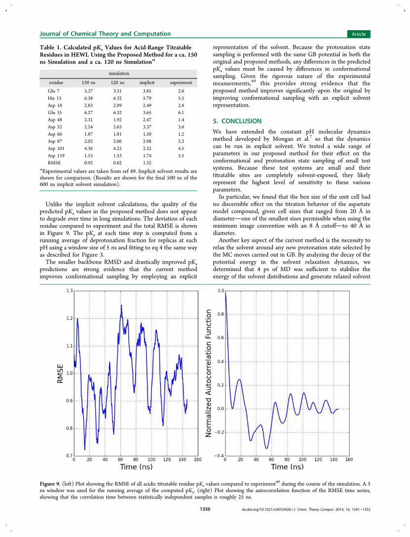
Unlike the implicit solvent calculations, the quality of thepredicted pKa values in the proposed method does not appearto degrade over time in long simulations. The deviation of eachresidue compared to experiment and the total RMSE is shownin Figure 9. The pKa at each time step is computed from arunning average of deprotonation fraction for replicas at eachpH using a window size of 5 ns and fitting to eq 4 the same wayas described for Figure 3.The smaller backbone RMSD and drastically improved pKa

predictions are strong evidence that the current methodimproves conformational sampling by employing an explicit

representation of the solvent. Because the protonation statesampling is performed with the same GB potential in both theoriginal and proposed methods, any differences in the predictedpKa values must be caused by differences in conformationalsampling. Given the rigorous nature of the experimentalmeasurements,49 this provides strong evidence that theproposed method improves significantly upon the original byimproving conformational sampling with an explicit solventrepresentation.

5. CONCLUSION

We have extended the constant pH molecular dynamicsmethod developed by Mongan et al.7 so that the dynamicscan be run in explicit solvent. We tested a wide range ofparameters in our proposed method for their effect on theconformational and protonation state sampling of small testsystems. Because these test systems are small and theirtitratable sites are completely solvent-exposed, they likelyrepresent the highest level of sensitivity to these variousparameters.In particular, we found that the box size of the unit cell had

no discernible effect on the titration behavior of the aspartatemodel compound, given cell sizes that ranged from 20 Å indiameterone of the smallest sizes permissible when using theminimum image convention with an 8 Å cutoffto 40 Å indiameter.Another key aspect of the current method is the necessity to

relax the solvent around any new protonation state selected bythe MC moves carried out in GB. By analyzing the decay of thepotential energy in the solvent relaxation dynamics, wedetermined that 4 ps of MD was sufficient to stabilize theenergy of the solvent distributions and generate relaxed solvent

Table 1. Calculated pKa Values for Acid-Range TitratableResidues in HEWL Using the Proposed Method for a ca. 150ns Simulation and a ca. 120 ns Simulationa

simulation

residue 150 ns 120 ns implicit experiment

Glu 7 3.37 3.31 3.85 2.6His 15 6.38 6.32 5.79 5.5Asp 18 2.83 2.89 2.49 2.8Glu 35 6.27 6.32 3.65 6.1Asp 48 2.31 1.92 2.47 1.4Asp 52 2.24 2.63 3.37 3.6Asp 66 1.87 1.81 1.50 1.2Asp 87 2.02 2.06 2.98 2.2Asp 101 4.36 4.25 2.32 4.5Asp 119 1.53 1.53 1.74 3.5RMSE 0.92 0.82 1.32

aExperimental values are taken from ref 49. Implicit solvent results areshown for comparison. (Results are shown for the final 500 ns of the600 ns implicit solvent simulation).

Figure 9. (left) Plot showing the RMSE of all acidic titratable residue pKa values compared to experiment49 during the course of the simulation. A 5ns window was used for the running average of the computed pKa. (right) Plot showing the autocorrelation function of the RMSE time series,showing that the correlation time between statistically independent samples is roughly 25 ns.



conformations whose energies are uncorrelated from the initialarrangements. However, given the expense of such a longrelaxation period, we investigated using fewer relaxation stepsto increase the simulation efficiency and found shorter timesdown to 0.2 pshad no measurable effect on the calculatedpKa and very little effect on the solvent distribution around themodel cysteine compound.Further tests on a small pentapeptide test system with two

titratable sites (ACFCA) showed the importance of using pH-REMD over conventional CpHMD with the proposed method.While we showed that the enhanced protonation state samplingof pH-REMD results in smoother titration curves for complexproteins in implicit solvent,24 even the simplest systems inexplicit solvent require pH-REMD to obtain a smooth titrationcurve.We tested the proposed method on HEWL, a very common

pKa benchmark system. We found that the proposed method ofusing GB implicit solvent to evaluate protonation state changesand explicit solvent to propagate dynamics yielded stabletrajectories whose predicted pKa values agreed well withexperiment. Our results show that using the proposed methodleads to a significant improvement in how systems are modeledat constant pH compared to the original method that used GBto propagate system dynamics.Often, the most interesting titratable residues in biological

systems have a large pKa shift compared to the modelcompound. These highly perturbed residues have environmentsdrastically different than the one provided by bulk solvent, andthe conformational sampling must be both accurate andextensive to yield accurate pKa predictions. In future work wewill explore the use of enhanced sampling techniques inconjunction with pH-REMD in an attempt to improve theefficiency of the conformational sampling in explicit solvent,such as accelerated MD and temperature-based REMD.

■ AUTHOR INFORMATIONCorresponding Author*E-mail: [email protected] authors declare no competing financial interest.

■ ACKNOWLEDGMENTSJ.M.S. gratefully acknowledges support from the NationalScience Foundation (NSF) GRFP award, computationalsupport from NCSA BlueWaters and the University of FloridaHigh Performance Computing center, and the Extreme Scienceand Engineering Discovery Environment (XSEDE), which issupported by National Science Foundation Grant No. OCI-1053575. The authors acknowledge support from NSF ACI-1147910 and ACI-1036208 to A.E.R. and National Institutes ofHealth (NIH) GM62248 to D.M.Y.

■ REFERENCES(1) Garcia-Moreno, B. J. Biol. 2009, 8, 98.(2) Perutz, M. F. Science 1978, 201, 1187−1191.(3) Alexov, E.; Mehler, E. L.; Baker, N.; Huang, Y.; Milletti, F.;Nielsen, J. E.; Farrell, D.; Carstensen, T.; Olsson, M. H. M.; Shen, J.K.; Warwicker, J.; Williams, S.; Word, J. M. Proteins 2011, 79, 3260−3275.(4) Baptista, A. M.; Martel, P. J.; Petersen, S. B. Proteins 1997, 27,523−544.(5) Baptista, A. M.; Teixeira, V. H.; Soares, C. M. J. Chem. Phys. 2002,117, 4184−4200.

(6) Lee, M. S.; Salsbury, F. R., Jr.; Brooks, C. L., III Proteins 2004, 56,738−752.(7) Mongan, J.; Case, D. A.; McCammon, J. A. J. Comput. Chem.2004, 25, 2038−2048.(8) Khandogin, J.; Brooks, C. L., III Biophys. J. 2005, 89, 141−157.(9) Wallace, J. A.; Shen, J. K. J. Chem. Theory Comput. 2011, 7, 2617−2629.(10) Goh, G. B.; Knight, J. L.; Brooks, C. L. J. Chem. Theory Comput.2012, 8, 36−46.(11) Donnini, S.; Tegeler, F.; Groenhof, G.; Grubmuller, H. J. Chem.Theory Comput. 2011, 7, 1962−1978.(12) Itoh, S. G.; Damjanovic, A.; Brooks, B. R. Proteins 2011, 79,3420−3436.(13) Walczak, A. M.; Antosiewicz, J. M. Phys. Rev. E 2002, 66,051911.(14) Burgi, R.; Kollman, P. A.; van Gunsteren, W. F. Proteins 2002,47, 469−480.(15) Machuqueiro, M.; Baptista, A. M. Proteins 2011, 79, 3437−3447.(16) Zgarbova, M.; Otyepka, M.; Sponer, J.; Mladek, A.; Banas, P.;Cheatham, T. E., III; JureCka, P. J. Chem. Theory Comput. 2011, 7,2886−2902.(17) Cheatham, T. E., III; A.Young, M. Biopolymers 2001, 56, 232−256.(18) Varnai, P.; Djuranovic, D.; Lavery, R.; Hartmann, B. NucleicAcids Res. 2002, 30, 5398−5406.(19) Hornak, V.; Abel, R.; Okur, A.; Strockbine, B.; Roitberg, A.;Simmerling, C. Proteins 2006, 65, 712−725.(20) Klepeis, J. L.; Lindorff-Larsen, K.; Dror, R. O.; Shaw, D. E. Curr.Opin. Struct. Biol. 2009, 19, 120−127.(21) Srivastava, J.; Barber, D. L.; Jacobson, M. P. Physiology 2007, 22,30−39.(22) Frantz, C.; Barreiro, G.; Dominguez, L.; Xiaoming, C.; Eddy, R.;Condeelis, J.; Kelly, M. J. S.; Jacobson, M. P.; Barber, D. L. J. Cell Biol.2008, 183, 865−871.(23) Di Russo, N.; Estrin, D. A.; Martí, M. A.; Roitberg, A. E. PLoSComput. Biol. 2012, 8, 1−9.(24) Swails, J. M.; Roitberg, A. E. J. Chem. Theory Comput. 2012, 8,4393−4404.(25) Wallace, J. A.; Shen, J. K. J. Chem. Phys. 2012, 137, 184105.(26) Machuqueiro, M.; Baptista, A. M. Proteins 2008, 72, 289−298.(27) Baptista, A. M.; Soares, C. M. J. Phys. Chem. B 2001, 105, 293−309.(28) Manousiouthakis, V. I.; Deem, M. W. J. Chem. Phys. 1999, 110,2753−2756.(29) Gregory D., Hawkins; C., C.; Truhlar, D. Chem. Phys. Lett. 1995,246, 122−129.(30) Hawkins, G. D.; Cramer, C. J.; Truhlar, D. G. J. Phys. Chem.1996, 100, 19824−19839.(31) Onufriev, A.; Bashford, D.; Case, D. A. Proteins 2004, 55, 383−394.(32) Mongan, J.; Simmerling, C.; McCammon, J. A.; Case, D. A.;Onufriev, A. J. Chem. Theory Comput. 2007, 3, 156−169.(33) Shang, Y.; Nguyen, H.; Wickstrom, L.; Okur, A.; Simmerling, C.J. Mol. Graphics 2011, 29, 676−684.(34) Williams, S. L.; de Oliveira, C. A. F.; McCammon, J. A. J. Chem.Theory Comput. 2010, 6, 560−568.(35) Bogusz, S.; Cheatham, T. E., III; Brooks, B. R. J. Chem. Phys.1998, 108, 7070−7084.(36) Rocklin, G. J.; Mobley, D. L.; Dill, K. A.; Hunenberger, P. H. J.Chem. Phys. 2013, 139, 184103.(37) Gotz, A.; Williamson, M. J.; Xu, D.; Poole, D.; Le Grand, S.;Walker, R. C. J. Chem. Theory Comput. 2012, 8, 1542.(38) Artymiuk, P. J.; Blake, C. C. F.; W., R. D.; S., W. K. Acta Cryst. B1982, 38, 778−783.(39) Jorgensen, W. L.; Chandrasekhar, J.; Madura, J. D.; Impey, R.W.; Klein, M. L. J. Chem. Phys. 1983, 79, 926−935.(40) Walsh, M. A.; Schneider, T. R.; Sieker, L. C.; Dauter, Z.;Lamzin, V. S.; Wilson, K. S. Acta Crystallogr. D 1998, 54, 522−546.



mailto:[email protected]

(41) Case, D. A.; Darden, T. A.; Cheatham III, T. E.; Simmerling, C.L.; Wang, J.; Duke, R. E.; Luo, R.; Walker, R. C.; Zhang, W.; Merz, K.M.; Roberts, B.; Hayik, S.; Roitberg, A.; Seabra, G.; Swails, J.; Gotz, A.W.; Kolossvary, I.; Wong, K. F.; Paesani, F.; Vanicek, J.; Wolf, R. M.;Liu, J.; Wu, X.; Brozell, S. R.; Steinbrecher, T.; Gohlke, H.; Cai, Q.; Ye,X.; Wang, J.; Hsieh, M.-J.; Cui, G.; Roe, D. R.; Mathews, D. H.; Seetin,M. G.; Salomon-Ferrer, C., Sagui, R.; ; Babin, V.; Luchko, T.; Gusarov,S.; Kovalenko, A.; Kollman, P. A. AMBER 12; University of California:San Francisco, 2012.(42) Uberuaga, B. P.; Anghel, M.; Voter, A. F. J. Chem. Phys. 2004,120, 6363−6374.(43) Sindhikara, D. J.; Kim, S.; Voter, A. F.; Roitberg, A. E. J. Chem.Theory Comput. 2009, 5, 1624−1631.(44) Ryckaert, J. P.; Ciccotti, G.; Berendsen, H. J. C. J. Comput. Phys.1977, 23, 327−341.(45) Miyamoto, S.; Kollman, P. A. J. Comput. Chem. 1992, 13, 952−962.(46) Darden, T.; York, D.; Pedersen, L. J. Chem. Phys. 1993, 98,10089−10092.(47) Essmann, U.; Perera, L.; Berkowitz, M. L.; Darden, T.; Hsing,L.; Pedersen, L. G. J. Chem. Phys. 1995, 103, 8577−8593.(48) Cheatham, T. E., III Curr. Opin. Struct. Biol. 2004, 14, 360−367.(49) Webb, H.; Tynan-Connolly, B. M.; Lee, G. M.; Farrell, D.;O’Meara, F.; Sondergaard, C. R.; Teilum, K.; Hewage, C.; McIntosh,L. P.; Nielsen, J. E. Proteins 2011, 79, 685−702.(50) Takahashi, T.; Nakamura, H.; Wada, A. Biopolymers 1992, 32,897−909.(51) Bartik, K.; Redfield, C.; Dobson, C. M. Biophys. J. 1994, 66,1180−1184.(52) Demchuk, E.; Wade, R. C. J. Phys. Chem. 1996, 100, 17373−17387.



constant ph replica exchange molecular dynamics in

Documents