CONGA: Distributed Congestion-Aware Load Balancing

for Datacenters

Mohammad Alizadeh†, Tom Edsall†, Sarang Dharmapurikar†, Ramanan Vaidyanathan†,Kevin Chu†, Andy Fingerhut†, Vinh The Lam‡, Francis Matus†, Rong Pan†,

Navindra Yadav†, George Varghese§

†Cisco Systems ‡Google §Microsoft

August 9, 2014

Abstract

We present the design, implementation, and evaluation of CONGA, a network-based distributedcongestion-aware load balancing mechanism for datacenters. CONGA exploits recent trends includingthe use of regular Clos topologies and overlays for network virtualization. It splits TCP flows into flowlets,estimates real-time congestion on fabric paths, and allocates flowlets to paths based on feedback fromremote switches. This enables CONGA to efficiently balance load and seamlessly handle asymmetry,without requiring any TCP modifications. CONGA has been implemented in custom ASICs as part ofa new datacenter fabric. In testbed experiments, CONGA has 5× better flow completion times thanECMP even with a single link failure and achieves 2–8× better throughput than MPTCP in Incastscenarios. Further, the Price of Anarchy for CONGA is provably small in Leaf-Spine topologies; henceCONGA is nearly as effective as a centralized scheduler while being able to react to congestion inmicroseconds. Our main thesis is that datacenter fabric load balancing is best done in the network, andrequires global schemes such as CONGA to handle asymmetry.

Categories and Subject Descriptors: C.2.1 [Computer-Communication Networks]: Network Archi-tecture and DesignKeywords: Datacenter fabric; Load balancing; Distributed

1 Introduction

Datacenter networks being deployed by cloud providers as well as enterprises must provide large bisectionbandwidth to support an ever increasing array of applications, ranging from financial services to big-data analytics. They also must provide agility, enabling any application to be deployed at any server, inorder to realize operational efficiency and reduce costs. Seminal papers such as VL2 [17] and Portland [1]showed how to achieve this with Clos topologies, Equal Cost MultiPath (ECMP) load balancing, andthe decoupling of endpoint addresses from their location. These design principles are followed by nextgeneration overlay technologies that accomplish the same goals using standard encapsulations such asVXLAN [34] and NVGRE [44].

However, it is well known [2, 40, 8, 26, 43, 9] that ECMP can balance load poorly. First, becauseECMP randomly hashes flows to paths, hash collisions can cause significant imbalance if there are afew large flows. More importantly, ECMP uses a purely local decision to split traffic among equal costpaths without knowledge of potential downstream congestion on each path. Thus ECMP fares poorlywith asymmetry caused by link failures that occur frequently and are disruptive in datacenters [16, 33].For instance, the recent study by Gill et al. [16] shows that failures can reduce delivered traffic by up to40% despite built-in redundancy.

Broadly speaking, the prior work on addressing ECMP’s shortcomings can be classified as either cen-tralized scheduling (e.g., Hedera [2]), local switch mechanisms (e.g., Flare [26]), or host-based transport

1

Centralized   Distributed  (e.g.,  Hedera,  B4,  SWAN)  slow  to  react  for  DCs  

Local      (Stateless  or  Conges6on-­‐Aware)    

(e.g.,  ECMP,  Flare,  LocalFlow)  Poor  with  asymmetry,  

especially  with  TCP  traffic  

Global,  Conges6on-­‐Aware  

   In-­‐Network      Host-­‐Based  (e.g.,  MPTCP)  Hard  to  deploy,  increases  Incast  

 General,  Link  State  Complex,  hard  to  

deploy  

Leaf  to  Leaf    Near-­‐op>mal  for  2-­‐>er,  

deployable  with  an  overlay  

 Per  Flow    Per  Flowlet  (CONGA)    Per  Packet  Subop>mal  for  “heavy”    

flow  distribu>ons  (with  large  flows)  No  TCP  modifica>ons,  

resilient  to  flow  distribu>on    Op>mal,  needs  

reordering-­‐resilient  TCP  

Figure 1: Design space for load balancing.

protocols (e.g., MPTCP [40]). These approaches all have important drawbacks. Centralized schemesare too slow for the traffic volatility in datacenters [27, 7] and local congestion-aware mechanisms aresuboptimal and can perform even worse than ECMP with asymmetry (§2.4). Host-based methods suchas MPTCP are challenging to deploy because network operators often do not control the end-host stack(e.g., in a public cloud) and even when they do, some high performance applications (such as low latencystorage systems [38, 6]) bypass the kernel and implement their own transport. Further, host-based loadbalancing adds more complexity to an already complex transport layer burdened by new requirementssuch as low latency and burst tolerance [3] in datacenters. As our experiments with MPTCP show, thiscan make for brittle performance (§5).

Thus from a philosophical standpoint it is worth asking: Can load balancing be done in the networkwithout adding to the complexity of the transport layer? Can such a network-based approach computeglobally optimal allocations, and yet be implementable in a realizable and distributed fashion to allowrapid reaction in microseconds? Can such a mechanism be deployed today using standard encapsu-lation formats? We seek to answer these questions in this paper with a new scheme called CONGA(for Congestion Aware Balancing). CONGA has been implemented in custom ASICs for a major newdatacenter fabric product line. While we report on lab experiments using working hardware togetherwith simulations and mathematical analysis, customer trials are scheduled in a few months as of thetime of this writing.

Figure 1 surveys the design space for load balancing and places CONGA in context by following thethick red lines through the design tree. At the highest level, CONGA is a distributed scheme to allowrapid round-trip timescale reaction to congestion to cope with bursty datacenter traffic [27, 7]. CONGAis implemented within the network to avoid the deployment issues of host-based methods and additionalcomplexity in the transport layer. To deal with asymmetry, unlike earlier proposals such as Flare [26]and LocalFlow [43] that only use local information, CONGA uses global congestion information, a designchoice justified in detail in §2.4.

Next, the most general design would sense congestion on every link and send generalized link statepackets to compute congestion-sensitive routes [15, 47, 50, 35]. However, this is an N-party protocol withcomplex control loops, likely to be fragile and hard to deploy. Recall that the early ARPANET movedbriefly to such congestion-sensitive routing and then returned to static routing, citing instability as areason [30]. CONGA instead uses a 2-party “leaf-to-leaf” mechanism to convey path-wise congestionmetrics between pairs of top-of-the-rack switches (also termed leaf switches) in a datacenter fabric.The leaf-to-leaf scheme is provably near-optimal in typical 2-tier Clos topologies (henceforth calledLeaf-Spine), simple to analyze, and easy to deploy. In fact, it is deployable in datacenters today withstandard overlay encapsulations (VXLAN [34] in our implementation) which are already being used toenable workload agility [32].

2

With the availability of very high-density switching platforms for the spine (or core) with 100s of40Gbps ports, a 2-tier fabric can scale upwards of 20,000 10Gbps ports.1 This design point coversthe needs of the overwhelming majority of enterprise datacenters, which are the primary deploymentenvironments for CONGA.

Finally, in the lowest branch of the design tree, CONGA is constructed to work with flowlets [26]to achieve a higher granularity of control and resilience to the flow size distribution while not requiringany modifications to TCP. Of course, CONGA could also be made to operate per packet by using a verysmall flowlet inactivity gap (see §3.4) to perform optimally with a future reordering-resilient TCP.

In summary, our major contributions are:

• We design (§3) and implement (§4) CONGA, a distributed congestion-aware load balancing mech-anism for datacenters. CONGA is immediately deployable, robust to asymmetries caused by linkfailures, reacts to congestion in microseconds, and requires no end-host modifications.

• We extensively evaluate (§5) CONGA with a hardware testbed and packet-level simulations. Weshow that even with a single link failure, CONGA achieves more than 5× better flow completion timeand 2× better job completion time respectively for a realistic datacenter workload and a standardHadoop Distributed File System benchmark. CONGA is at least as good as MPTCP for loadbalancing while outperforming MPTCP by 2–8× in Incast [46, 11] scenarios.

• We analyze (§6) CONGA and show that it is nearly optimal in 2-tier Leaf-Spine topologies using“Price of Anarchy” [39] analysis. We also prove that load balancing behavior and the effectivenessof flowlets depends on the coefficient of variation of the flow size distribution.

2 Design Decisions

This section describes the insights that inform CONGA’s major design decisions. We begin with thedesired properties that have guided our design. We then revisit the design decisions shown in Figure 1in more detail from the top down.

2.1 Desired Properties

CONGA is an in-network congestion-aware load balancing mechanism for datacenter fabrics. In design-ing CONGA, we targeted a solution with a number of key properties:

1. Responsive: Datacenter traffic is very volatile and bursty [17, 27, 7] and switch buffers are shal-low [3]. Thus, with CONGA, we aim for rapid round-trip timescale (e.g., 10s of microseconds)reaction to congestion.

2. Transport independent: As a network mechanism, CONGA must be oblivious to the transportprotocol at the end-host (TCP, UDP, etc). Importantly, it should not require any modifications toTCP.

3. Robust to asymmetry: CONGA must handle asymmetry due to link failures (which have beenshown to be frequent and disruptive in datacenters [16, 33]) or high bandwidth flows that are notwell balanced.

4. Incrementally deployable: It should be possible to apply CONGA to only a subset of the trafficand only a subset of the switches.

5. Optimized for Leaf-Spine topology: CONGA must work optimally for 2-tier Leaf-Spine topolo-gies (Figure 4) that cover the needs of most enterprise datacenter deployments, though it shouldalso benefit larger topologies.

1For example, spine switches with 576 40Gbps ports can be paired with typical 48-port leaf switches to enable non-blockingfabrics with 27,648 10Gbps ports.

3

2.2 Why Distributed Load Balancing?

The distributed approach we advocate is in stark contrast to recently proposed centralized traffic engi-neering designs [2, 8, 22, 20]. This is because of two important features of datacenters. First, datacentertraffic is very bursty and unpredictable [17, 27, 7]. CONGA reacts to congestion at RTT timescales(∼100µs) making it more adept at handling high volatility than a centralized scheduler. For example,the Hedera scheduler in [2] runs every 5 seconds; but it would need to run every 100ms to approach theperformance of a distributed solution such as MPTCP [40], which is itself outperformed by CONGA(§5). Second, datacenters use very regular topologies. For instance, in the common Leaf-Spine topology(Figure 4), all paths are exactly two-hops. As our experiments (§5) and analysis (§6) show, distributeddecisions are close to optimal in such regular topologies.

Of course, a centralized approach is appropriate for WANs where traffic is stable and predictable andthe topology is arbitrary. For example, Google’s inter-datacenter traffic engineering algorithm needs torun just 540 times per day [22].

2.3 Why In-Network Load Balancing?

Continuing our exploration of the design space (Figure 1), the next question is where should datacenterfabric load balancing be implemented — the transport layer at the end-hosts or the network?

The state-of-the-art multipath transport protocol, MPTCP [40], splits each connection into mul-tiple (e.g., 8) sub-flows and balances traffic across the sub-flows based on perceived congestion. Ourexperiments (§5) show that while MPTCP is effective for load balancing, its use of multiple sub-flowsactually increases congestion at the edge of the network and degrades performance in Incast scenarios(Figure 13). Essentially, MPTCP increases the burstiness of traffic as more sub-flows contend at thefabric’s access links. Note that this occurs despite MPTCP’s coupled congestion control algorithm [49]which is designed to handle shared bottlenecks, because while the coupled congestion algorithm works ifflows are in steady-state, in realistic datacenter workloads, many flows are short-lived and transient [17].

The larger architectural point however is that datacenter fabric load balancing is too specific to beimplemented in the transport stack. Datacenter fabrics are highly-engineered, homogenous systems [1,33]. They are designed from the onset to behave like a giant switch [17, 1, 24], much like the internalfabric within large modular switches. Binding the fabric’s load balancing behavior to the transport stackwhich already needs to balance multiple important requirements (e.g., high throughput, low latency, andburst tolerance [3]) is architecturally unappealing. Further, some datacenter applications such as highperformance storage systems bypass the kernel altogether [38, 6] and hence cannot use MPTCP.

2.4 Why Global Congestion Awareness?

Next, we consider local versus global schemes (Figure 1). Handling asymmetry essentially requiresnon-local knowledge about downstream congestion at the switches. With asymmetry, a switch cannotsimply balance traffic based on the congestion of its local links. In fact, this may lead to even worseperformance than a static scheme such as ECMP (which does not consider congestion at all) because ofpoor interaction with TCP’s control loop.

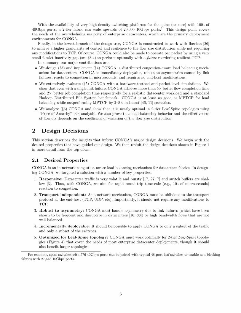
As an illustration, consider the simple asymmetric scenario in Figure 2. Leaf L0 has 100Gbps ofTCP traffic demand to Leaf L1. Static ECMP splits the flows equally, achieving a throughput of 90Gbpsbecause the flows on the lower path are bottlenecked at the 40Gbps link (S1, L1). Local congestion-awareload balancing is actually worse with a throughput of 80Gbps. This is because as TCP slows down theflows on the lower path, the link (L0, S1) appears less congested. Hence, paradoxically, the local schemeshifts more traffic to the lower link until the throughput on the upper link is also 40 Gbps. This exampleillustrates a fundamental limitation of any local scheme (such as Flare [26], LocalFlow [43], and packet-spraying [9]) that strictly enforces an equal traffic split without regard for downstream congestion. Ofcourse, global congestion-aware load balancing (as in CONGA) does not have this issue.

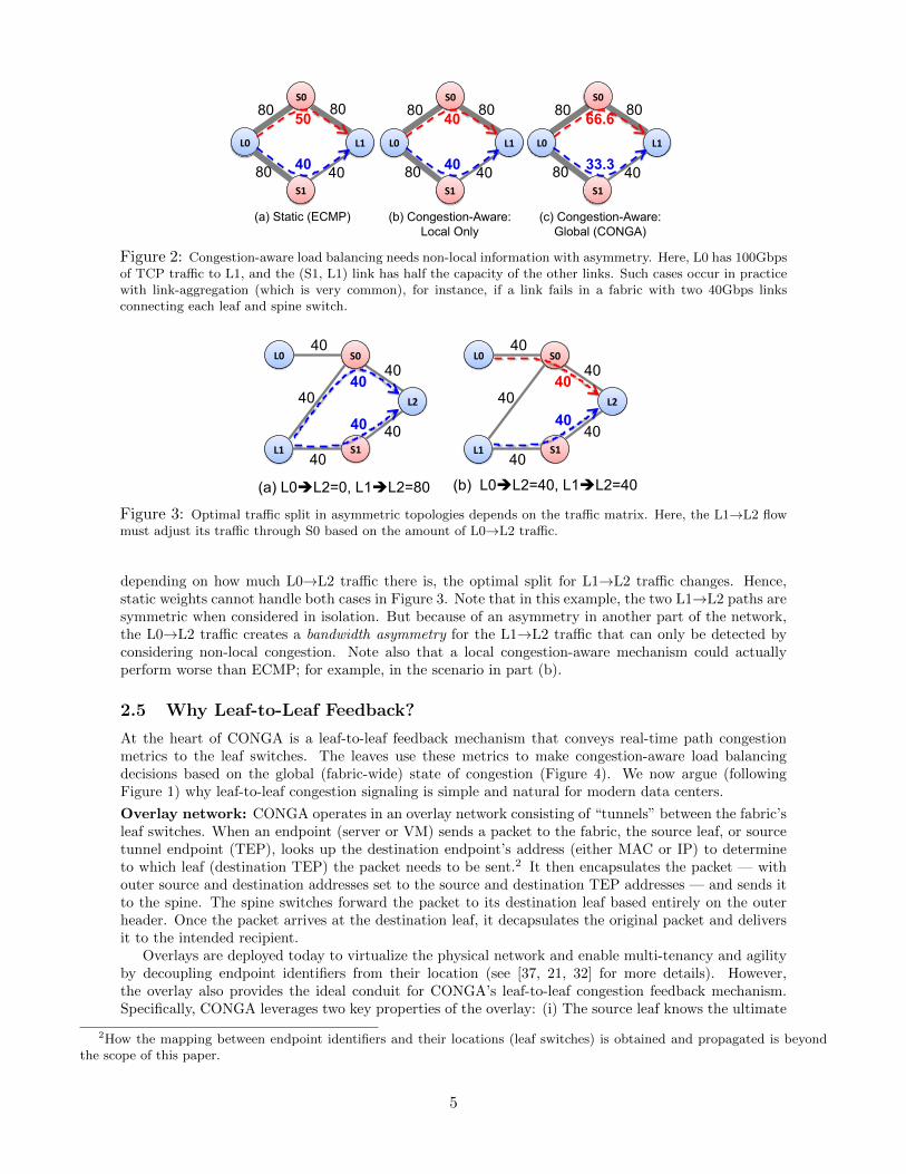
The reader may wonder if asymmetry can be handled by some form of oblivious routing [31] suchas weighted random load balancing with weights chosen according to the topology. For instance, in theabove example we could give the lower path half the weight of the upper path and achieve the sametraffic split as CONGA. While this works in this case, it fails in general because the “right” traffic splitsin asymmetric topologies depend also on the traffic matrix, as shown by the example in Figure 3. Here,

4

L0   L1  

S0  

S1  

80

80

80

40

50

40

(a) Static (ECMP)

L0   L1  

S0  

S1  

80

80

80

40

40

40

(b) Congestion-Aware: Local Only

L0   L1  

S0  

S1  

80

80

80

40

66.6

33.3

(c) Congestion-Aware: Global (CONGA)

Figure 2: Congestion-aware load balancing needs non-local information with asymmetry. Here, L0 has 100Gbpsof TCP traffic to L1, and the (S1, L1) link has half the capacity of the other links. Such cases occur in practicewith link-aggregation (which is very common), for instance, if a link fails in a fabric with two 40Gbps linksconnecting each leaf and spine switch.

L2  

L1  

S0  

S1  

40

40

40

40

L0  

40 40

40 L2  

L1  

S0  

S1  

40

40

40

40

L0  

40

40

40

(a) L0L2=0, L1L2=80 (b) L0L2=40, L1L2=40

Figure 3: Optimal traffic split in asymmetric topologies depends on the traffic matrix. Here, the L1→L2 flowmust adjust its traffic through S0 based on the amount of L0→L2 traffic.

depending on how much L0→L2 traffic there is, the optimal split for L1→L2 traffic changes. Hence,static weights cannot handle both cases in Figure 3. Note that in this example, the two L1→L2 paths aresymmetric when considered in isolation. But because of an asymmetry in another part of the network,the L0→L2 traffic creates a bandwidth asymmetry for the L1→L2 traffic that can only be detected byconsidering non-local congestion. Note also that a local congestion-aware mechanism could actuallyperform worse than ECMP; for example, in the scenario in part (b).

2.5 Why Leaf-to-Leaf Feedback?

At the heart of CONGA is a leaf-to-leaf feedback mechanism that conveys real-time path congestionmetrics to the leaf switches. The leaves use these metrics to make congestion-aware load balancingdecisions based on the global (fabric-wide) state of congestion (Figure 4). We now argue (followingFigure 1) why leaf-to-leaf congestion signaling is simple and natural for modern data centers.

Overlay network: CONGA operates in an overlay network consisting of “tunnels” between the fabric’sleaf switches. When an endpoint (server or VM) sends a packet to the fabric, the source leaf, or sourcetunnel endpoint (TEP), looks up the destination endpoint’s address (either MAC or IP) to determineto which leaf (destination TEP) the packet needs to be sent.2 It then encapsulates the packet — withouter source and destination addresses set to the source and destination TEP addresses — and sends itto the spine. The spine switches forward the packet to its destination leaf based entirely on the outerheader. Once the packet arrives at the destination leaf, it decapsulates the original packet and deliversit to the intended recipient.

Overlays are deployed today to virtualize the physical network and enable multi-tenancy and agilityby decoupling endpoint identifiers from their location (see [37, 21, 32] for more details). However,the overlay also provides the ideal conduit for CONGA’s leaf-to-leaf congestion feedback mechanism.Specifically, CONGA leverages two key properties of the overlay: (i) The source leaf knows the ultimate

2How the mapping between endpoint identifiers and their locations (leaf switches) is obtained and propagated is beyondthe scope of this paper.

5

Source Leaf

Spine Tier

Destination Leaf

0 1 3

Gap

Flowlet  Detec*on  

Conges*on  Feedback  

2

Overlay  Network  LB  Decision  

Per-­‐link  Conges*on  Measurement  

?

Figure 4: CONGA architecture. The source leaf switch detects flowlets and routes them via the least congestedpath to the destination using congestion metrics obtained from leaf-to-leaf feedback. Note that the topology couldbe asymmetric.

destination leaf for each packet, in contrast to standard IP forwarding where the switches only knowthe next-hops. (ii) The encapsulated packet has an overlay header (VXLAN [34] in our implementation)which can be used to carry congestion metrics between the leaf switches.

Congestion feedback: The high-level mechanism is as follows. Each packet carries a congestionmetric in the overlay header that represents the extent of congestion the packet experiences as it traversesthrough the fabric. The metric is updated hop-by-hop and indicates the utilization of the most congestedlink along the packet’s path. This information is stored at the destination leaf on a per source leaf, perpath basis and is opportunistically fed back to the source leaf by piggybacking on packets in the reversedirection. There may be, in general, 100s of paths in a multi-tier topology. Hence, to reduce state, thedestination leaf aggregates congestion metrics for one or more paths based on a generic identifier calledthe Load Balancing Tag that the source leaf inserts in packets (see §3 for details).

2.6 Why Flowlet Switching for Datacenters?

CONGA also employs flowlet switching, an idea first introduced by Kandula et al. [26]. Flowlets arebursts of packets from a flow that are separated by large enough gaps (see Figure 4). Specifically, ifthe idle interval between two bursts of packets is larger than the maximum difference in latency amongthe paths, then the second burst can be sent along a different path than the first without reorderingpackets. Thus flowlets provide a higher granularity alternative to flows for load balancing (withoutcausing reordering).

2.6.1 Measurement analysis

Flowlet switching has been shown to be an effective technique for fine-grained load balancing acrossInternet paths [26], but how does it perform in datacenters? On the one hand, the very high bandwidthof internal datacenter flows would seem to suggest that the gaps needed for flowlets may be rare, limitingthe applicability of flowlet switching. On the other hand, datacenter traffic is known to be extremelybursty at short timescales (e.g., 10–100s of microseconds) for a variety of reasons such as NIC hardwareoffloads designed to support high link rates [28]. Since very small flowlet gaps suffice in datacenters tomaintain packet order (because the network latency is very low) such burstiness could provide sufficientflowlet opportunities.

We study the applicability of flowlet switching in datacenters using measurements from actual pro-duction datacenters. We instrument a production cluster with over 4500 virtualized and bare metal

6

0  0.2  0.4  0.6  0.8  1  

1.E+01   1.E+03   1.E+05   1.E+07   1.E+09  Frac%o

n  of  Data  By

tes  

Size  (Bytes)  

Flow  (250ms)  Flowlet  (500μs)  Flowlet  (100μs)  

Figure 5: Distribution of data bytes across transfer sizes for different flowlet inactivity gaps.

hosts across ∼30 racks of servers to obtain packet traces of traffic flows through the network core. Thecluster supports over 2000 diverse enterprise applications, including web, data-base, security, and busi-ness intelligence services. The captures are obtained by having a few leaf switches mirror traffic to ananalyzer without disrupting production traffic. Overall, we analyze more than 150GB of compressedpacket trace data.

Flowlet size: Figure 5 shows the distribution of the data bytes versus flowlet size for three choices offlowlet inactivity gap: 250ms, 500µs, and 100µs. Since it is unlikely that we would see a gap larger than250ms in the same application-level flow, the line “Flow (250ms)” essentially corresponds to how thebytes are spread across flows. The plot shows that balancing flowlets gives significantly more fine-grainedcontrol than balancing flows. Even with an inactivity gap of 500µs, which is quite large and poses littlerisk of packet reordering in datacenters, we see nearly two orders of magnitude reduction in the size oftransfers that cover most of the data: 50% of the bytes are in flows larger than ∼30MB, but this numberreduces to ∼500KB for “Flowlet (500µs)”.

Flowlet concurrency: Since the required flowlet inactivity gap is very small in datacenters, we expectthere to be a small number of concurrent flowlets at any given time. Thus, the implementation cost fortracking flowlets should be low. To quantify this, we measure the distribution of the number of distinct5-tuples in our packet trace over 1ms intervals. We find that the number of distinct 5-tuples (and thusflowlets) is small, with a median of 130 and a maximum under 300. Normalizing these numbers to theaverage throughput in our trace (∼15Gbps), we estimate that even for a very heavily loaded leaf switchwith say 400Gbps of traffic, the number of concurrent flowlets would be less than 8K. Maintaining atable for tracking 64K flowlets is feasible at low cost (§3.4).

3 Design

Figure 6 shows the system diagram of CONGA. The majority of the functionality resides at the leafswitches. The source leaf makes load balancing decisions based on per uplink congestion metrics, derivedby taking the maximum of the local congestion at the uplink and the remote congestion for the path(or paths) to the destination leaf that originate at the uplink. The remote metrics are stored in theCongestion-To-Leaf Table on a per destination leaf, per uplink basis and convey the maximum congestionfor all the links along the path. The remote metrics are obtained via feedback from the destination leafswitch, which opportunistically piggybacks values in its Congestion-From-Leaf Table back to the sourceleaf. CONGA measures congestion using the Discounting Rate Estimator (DRE), a simple modulepresent at each fabric link.

Load balancing decisions are made on the first packet of each flowlet. Subsequent packets use thesame uplink as long as the flowlet remains active (there is not a sufficiently long gap). The source leafuses the Flowlet Table to keep track of active flowlets and their chosen uplinks.

7

Leaf  A  (Sender)  

Flowlet  Table  

Conges7on-­‐To-­‐Leaf  Table  

Per-­‐uplink  DREs  

?LB  Decision  De

st  Leaf  

Uplink  0 1 k-­‐1  

B 52 3

Per-­‐link  DREs  in  Spine  

Leaf  B  (Receiver)  0 1 2 3

A→B  LBTag=2  CE=4  

B→A  FB_LBTag=1  FB_Metric=5  Reverse    Path  Pkt  

Forward    Path  Pkt  

Conges7on-­‐From-­‐Leaf  Table  

Source  Leaf  

LBTag  0 1 k-­‐1  

A 52 3

Figure 6: CONGA system diagram.

3.1 Packet format

CONGA leverages the VXLAN [34] encapsulation format used for the overlay to carry the followingstate:

• LBTag (4 bits): This field partially identifies the packet’s path. It is set by the source leaf to the(switch-local) port number of the uplink the packet is sent on and is used by the destination leafto aggregate congestion metrics before they are fed back to the source. For example, in Figure 6,the LBTag is 2 for both blue paths. Note that 4 bits is sufficient because the maximum number ofleaf uplinks in our implementation is 12 for a non-oversubscribed configuration with 48 × 10Gbpsserver-facing ports and 12× 40Gbps uplinks.

• CE (3 bits): This field is used by switches along the packet’s path to convey the extent of conges-tion.

• FB LBTag (4 bits) and FB Metric (3 bits): These two fields are used by destination leavesto piggyback congestion information back to the source leaves. FB LBTag indicates the LBTag thefeedback is for and FB Metric provides its associated congestion metric.

3.2 Discounting Rate Estimator (DRE)

The DRE is a simple module for measuring the load of a link(see Algorithm 1) The DRE maintains aregister, X, which is incremented for each packet sent over the link by the packet size in bytes, and isdecremented periodically (every Tdre) with a multiplicative factor α between 0 and 1: X ← X× (1−α).It is easy to show that X is proportional to the rate of traffic over the link; more precisely, if the trafficrate is R, then X ≈ R · τ , where τ = Tdre/α. The DRE algorithm is essentially a first-order low passfilter applied to packet arrivals, with a (1 − e−1) rise time of τ . The congestion metric for the link isobtained by quantizing X/Cτ to 3 bits (C is the link speed).

The DRE algorithm is similar to the widely used Exponential Weighted Moving Average (EWMA)mechanism. However, DRE has two key advantages over EWMA: (i) it can be implemented with just oneregister (whereas EWMA requires two); and (ii) the DRE reacts more quickly to traffic bursts (becauseincrements take place immediately upon packet arrivals) while retaining memory of past bursts.

8

Algorithm 1 DRE algorithm for measuring congestion

For each packet traversing the link:X ← X + packet.size (in bytes)

Periodically with period Tdre:X ← X × (1− α)

3.3 Congestion Feedback

CONGA uses a feedback loop between the source and destination leaf switches to populate the remotemetrics in the Congestion-To-Leaf Table at each leaf switch. We now describe the sequence of eventsinvolved (refer to Figure 6 for an example).

1. The source leaf sends the packet to the fabric with the LBTag field set to the uplink port taken bythe packet. It also sets the CE field to zero.

2. The packet is routed through the fabric to the destination leaf.3 As it traverses each link, its CEfield is updated if the link’s congestion metric (given by the DRE) is larger than the current valuein the packet.

3. The CE field of the packet received at the destination leaf gives the maximum link congestionalong the packet’s path. This needs to be fed back to the source leaf. But since a packet maynot be immediately available in the reverse direction, the destination leaf stores the metric in theCongestion-From-Leaf Table (on a per source leaf, per LBTag basis) while it waits for an opportunityto piggyback the feedback.

4. When a packet is sent in the reverse direction, one metric from the Congestion-From-Leaf Table isinserted in its FB LBTag and FB Metric fields for the source leaf. The metric is chosen in round-robin fashion while, as an optimization, favoring those metrics whose values have changed since thelast time they were fed back.

5. Finally, the source leaf parses the feedback in the reverse packet and updates the Congestion-To-LeafTable.

It is important to note that though we have described the forward and reverse packets separatelyfor simplicity, every packet simultaneously carries both a metric for its forward path and a feedbackmetric. Also, while we could generate explicit feedback packets, we decided to use piggybacking becausewe only need a very small number of packets for feedback. In fact, all metrics between a pair of leafswitches can be conveyed in at-most 12 packets (because there are 12 distinct LBTag values), with theaverage case being much smaller because the metrics only change at network round-trip timescales, notpacket-timescales (see the discussion in §3.6 regarding the DRE time constant).

Metric aging: A potential issue with not having explicit feedback packets is that the metrics maybecome stale if sufficient traffic does not exit for piggybacking. To handle this, a simple aging mechanismis added where a metric that has not been updated for a long time (e.g., 10ms) gradually decays to zero.This also guarantees that a path that appears to be congested is eventually probed again.

3.4 Flowlet Detection

Flowlets are detected and tracked in the leaf switches using the Flowlet Table according to Algo-rithm 2 Each entry of the table consists of a port number, a valid bit, and an age bit. When a packetarrives, we lookup an entry based on a hash of its 5-tuple. If the entry is valid (valid bit == 1), theflowlet is active and the packet is sent on the port indicated in the entry. If the entry is not valid, theincoming packet starts a new flowlet. In this case, we make a load balancing decision (as describedbelow) and cache the result in the table for use by subsequent packets. We also set the valid bit.

3If there are multiple valid next hops to the destination (as in Figure 6), the spine switches pick one using standard ECMPhashing.

9

Algorithm 2 Flowlet detection algorithm.

For each packet:ENTRY ← FLOWLET TABLE[ Hash(5-tuple) ]if ENTRY.valid bit == 1 then

The flowlet is active. Use uplink ENTRY.port for packet.else

Packet starts a new flowlet. Make load balancing decision and store the result in ENTRY.port.end ifENTRY.valid bit← 1ENTRY.age bit← 0

Periodically with period FLOWLET TIMEOUT:if ENTRY.age bit == 1 thenENTRY.valid bit← 0

end ifENTRY.age bit← 1

Flowlet entries time out using the age bit. Each incoming packet resets the age bit. A timerperiodically (every Tfl seconds) checks the age bit before setting it. If the age bit is set when the timerchecks it, then there have not been any packets for that entry in the last Tfl seconds and the entryexpires (the valid bit is set to zero). Note that a single age bit allows us to detect gaps between Tfl and2Tfl. While not as accurate as using full timestamps, this requires far fewer bits allowing us to maintaina very large number of entries in the table (64K in our implementation) at low cost.

Remark 1. Although with hashing, flows may collide in the Flowlet Table, this is not a big concern.Collisions simply imply some load balancing opportunities are lost which does not matter as long as thisdoes not occur too frequently.

3.5 Load Balancing Decision Logic

Load balancing decisions are made on the first packet of each flowlet (other packets use the port cachedin the Flowlet Table). For a new flowlet, we pick the uplink port that minimizes the maximum of thelocal metric (from the local DREs) and the remote metric (from the Congestion-To-Leaf Table). Ifmultiple uplinks are equally good, one is chosen at random with preference given to the port cached inthe (invalid) entry in the Flowlet Table; i.e., a flow only moves if there is a strictly better uplink thanthe one its last flowlet took.

3.6 Parameter Choices

CONGA has three main parameters: (i) Q, the number of bits for quantizing congestion metrics (§3.1);(ii) τ , the DRE time constant, given by Tdre/α (§3.2); and (iii) Tfl, the flowlet inactivity timeout (§3.4).We set these parameters experimentally. A control-theoretic analysis of CONGA is beyond the scopeof this paper, but our parameter choices strike a balance between the stability and responsiveness ofCONGA’s control loop while taking into consideration practical matters such as interaction with TCPand implementation cost (header requirements, table size, etc).

The parameters Q and τ determine the “gain” of CONGA’s control loop and exhibit importanttradeoffs. A large Q improves congestion metric accuracy, but if too large can make the leaf switchesover-react to minor differences in congestion causing oscillatory behavior. Similarly, a small τ makesthe DRE respond quicker, but also makes it more susceptible to noise from transient traffic bursts.Intuitively, τ should be set larger than the network RTT to filter the sub-RTT traffic bursts of TCP.The flowlet timeout, Tfl, can be set to the maximum possible leaf-to-leaf latency to guarantee no packetreordering. This value can be rather large though because of worst-case queueing delays (e.g., 13ms inour testbed), essentially disabling flowlets. Reducing Tfl presents a compromise between more packetreordering versus less congestion (fewer packet drops, lower latency) due to better load balancing.

10

32x10Gbps Leaf 0 Leaf 1

Spine 0 Spine 1

4x40Gbps 4x40Gbps

32x10Gbps

(a) Baseline (no failure)

32x10Gbps Leaf 0 Leaf 1

Spine 0 Spine 1

4x40Gbps

32x10Gbps

3x40Gbps

Link Failure

(b) With link failure

Figure 7: Topologies used in testbed experiments.

Overall, we have found CONGA’s performance to be fairly robust with: Q = 3 to 6, τ = 100µsto 500µs, and Tfl = 300µs to 1ms. The default parameter values for our implementation are: Q = 3,τ = 160µs, and Tfl = 500µs.

4 Implementation

CONGA has been implemented in custom switching ASICs for a major datacenter fabric product line.The implementation includes ASICs for both the leaf and spine nodes. The Leaf ASIC implementsflowlet detection, congestion metric tables, DREs, and the leaf-to-leaf feedback mechanism. The SpineASIC implements the DRE and its associated congestion marking mechanism. The ASICs provide state-of-the-art switching capacities. For instance, the Leaf ASIC has a non-blocking switching capacity of960Gbps in 28nm technology. CONGA’s implementation requires roughly 2.4M gates and 2.8Mbits ofmemory in the Leaf ASIC, and consumes negligible die area (< 2%).

5 Evaluation

In this section, we evaluate CONGA’s performance with a real hardware testbed as well as large-scalesimulations. Our testbed experiments illustrate CONGA’s good performance for realistic empiricalworkloads, Incast micro-benchmarks, and actual applications. Our detailed packet-level simulationsconfirm that CONGA scales to large topologies.

Schemes compared: We compare CONGA, CONGA-Flow, ECMP, and MPTCP [40], the state-of-the-art multipath transport protocol. CONGA and CONGA-Flow differ only in their choice of theflowlet inactivity timeout. CONGA uses the default value: Tfl = 500µs. CONGA-Flow howeveruses Tfl = 13ms which is greater than the maximum path latency in our testbed and ensures nopacket reordering. CONGA-Flow’s large timeout effectively implies one load balancing decision perflow, similar to ECMP. Of course, in contrast to ECMP, decisions in CONGA-Flow are informed by thepath congestion metrics. The rest of the parameters for both variants of CONGA are set as describedin §3.6. For MPTCP, we use MPTCP kernel v0.87 available on the web [36]. We configure MPTCP touse 8 sub-flows for each TCP connection, as Raiciu et al. [40] recommend.

5.1 Testbed

Our testbed consists of 64 servers and four switches (two leaves and two spines). As shown in Figure 7,the servers are organized in two racks (32 servers each) and attach to the leaf switches with 10Gbpslinks. In the baseline topology (Figure 7(a)), the leaf switches connect to each spine switch with two40Gbps uplinks. Note that there is a 2:1 oversubscription at the Leaf level, typical of today’s datacenterdeployments. We also consider the asymmetric topology in Figure 7(b) where one of the links betweenLeaf 1 and Spine 1 is down. The servers have 12-core Intel Xeon X5670 2.93GHz CPUs, 128GB of RAM,and 3 2TB 7200RPM HDDs.

11

0  0.2  0.4  0.6  0.8  1  

1.E+01   1.E+03   1.E+05   1.E+07   1.E+09  

CDF  

Size  (Bytes)  

Flow  Size  Bytes  

(a) Enterprise workload

0  0.2  0.4  0.6  0.8  1  

1.E+01   1.E+03   1.E+05   1.E+07   1.E+09  

CDF  

Size  (Bytes)  

Flow  Size  Bytes  

(b) Data-mining workload

Figure 8: Empirical traffic distributions. The Bytes CDF shows the distribution of traffic bytes across differentflow sizes.

5.2 Empirical Workloads

We begin with experiments with realistic workloads based on empirically observed traffic patterns indeployed datacenters. Specifically, we consider the two flow size distributions shown in Figure 8. Thefirst distribution is derived from packet traces from our own datacenters (§2.6) and represents a largeenterprise workload. The second distribution is from a large cluster running data mining jobs [17].Note that both distributions are heavy-tailed: A small fraction of the flows contribute most of the data.Particularly, the data-mining distribution has a very heavy tail with 95% of all data bytes belonging to∼3.6% of flows that are larger than 35MB.

We develop a simple client-server program to generate the traffic. The clients initiate 3 long-livedTCP connections to each server and request flows according to a Poisson process from randomly chosenservers. The request rate is chosen depending on the desired offered load and the flow sizes are sampledfrom one of the above distributions. All 64 nodes run both client and server processes. Since we areinterested in stressing the fabric’s load balancing, we configure the clients under Leaf 0 to only use theservers under Leaf 1 and vice-versa, thereby ensuring that all traffic traverses the Spine. Similar to priorwork [19, 4, 12], we use the flow completion time (FCT) as our main performance metric.

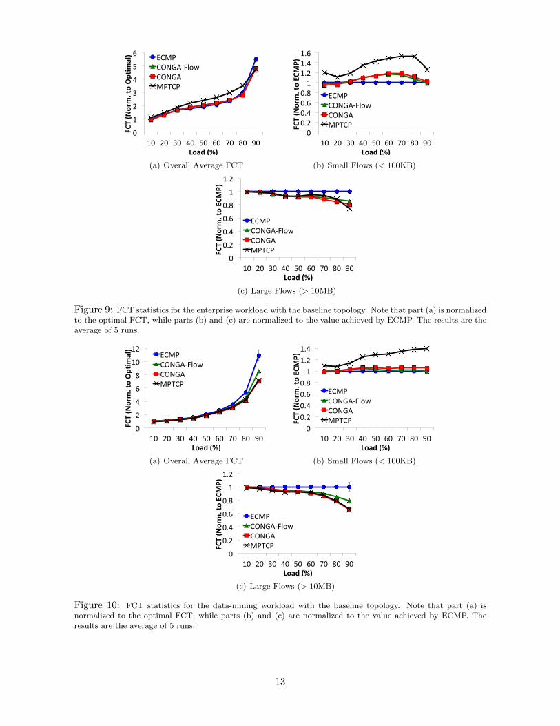
5.2.1 Baseline

Figures 9 and 10 show the results for the two workloads with the baseline topology (Figure 7(a)). Part(a) of each figure shows the overall average FCT for each scheme at traffic loads between 10–90%. Thevalues here are normalized to the optimal FCT that is achievable in an idle network. In parts (b) and(c), we break down the FCT for each scheme for small (< 100KB) and large (> 10MB) flows, normalizedto the value achieved by ECMP. Each data point is the average of 5 runs with the error bars showingthe range. (Note that the error bars are not visible at all data points.)

Enterprise workload: We find that the overall average FCT is similar for all schemes in the enterpriseworkload, except for MPTCP which is up to ∼25% worse than the others. MPTCP’s higher overallaverage FCT is because of the small flows, for which it is up to ∼50% worse than ECMP. CONGA andsimilarly CONGA-Flow are slightly worse for small flows (∼12–19% at 50–80% load), but improve FCTfor large flows by as much as ∼20%.

Data-mining workload: For the data-mining workload, ECMP is noticeably worse than the otherschemes at the higher load levels. Both CONGA and MPTCP achieve up to ∼35% better overallaverage FCT than ECMP. Similar to the enterprise workload, we find a degradation in FCT for smallflows with MPTCP compared to the other schemes.

Analysis: The above results suggest a tradeoff with MPTCP between achieving good load balancingin the core of the fabric and managing congestion at the edge. Essentially, while using 8 sub-flows perconnection helps MPTCP achieve better load balancing, it also increases congestion at the edge linksbecause the multiple sub-flows cause more burstiness. Further, as observed by Raiciu et al. [40], thesmall sub-flow window sizes for short flows increases the chance of timeouts. This hurts the performanceof short flows which are more sensitive to additional latency and packet drops. CONGA on the other

12

0  

1  

2  

3  

4  

5  

6  

10   20   30   40   50   60   70   80   90  

FCT  (Norm.  to  Op.

mal)  

Load  (%)  

ECMP  CONGA-­‐Flow  CONGA  MPTCP  

(a) Overall Average FCT

0  0.2  0.4  0.6  0.8  1  

1.2  1.4  1.6  

10   20   30   40   50   60   70   80   90  

FCT  (Norm.  to  EC

MP)  

Load  (%)  

ECMP  CONGA-­‐Flow  CONGA  MPTCP  

(b) Small Flows (< 100KB)

0  

0.2  

0.4  

0.6  

0.8  

1  

1.2  

10   20   30   40   50   60   70   80   90  

FCT  (Norm.  to  EC

MP)  

Load  (%)  

ECMP  CONGA-­‐Flow  CONGA  MPTCP  

(c) Large Flows (> 10MB)

Figure 9: FCT statistics for the enterprise workload with the baseline topology. Note that part (a) is normalizedto the optimal FCT, while parts (b) and (c) are normalized to the value achieved by ECMP. The results are theaverage of 5 runs.

0  

2  

4  

6  

8  

10  

12  

10   20   30   40   50   60   70   80   90  

FCT  (Norm.  to  Op.

mal)  

Load  (%)  

ECMP  CONGA-­‐Flow  CONGA  MPTCP  

(a) Overall Average FCT

0  0.2  0.4  0.6  0.8  1  

1.2  1.4  

10   20   30   40   50   60   70   80   90  

FCT  (Norm.  to  EC

MP)  

Load  (%)  

ECMP  CONGA-­‐Flow  CONGA  MPTCP  

(b) Small Flows (< 100KB)

0  

0.2  

0.4  

0.6  

0.8  

1  

1.2  

10   20   30   40   50   60   70   80   90  

FCT  (Norm.  to  EC

MP)  

Load  (%)  

ECMP  CONGA-­‐Flow  CONGA  MPTCP  

(c) Large Flows (> 10MB)

Figure 10: FCT statistics for the data-mining workload with the baseline topology. Note that part (a) isnormalized to the optimal FCT, while parts (b) and (c) are normalized to the value achieved by ECMP. Theresults are the average of 5 runs.

13

0  

2  

4  

6  

8  

10  

10   20   30   40   50   60   70  

FCT  (Norm.  to  Op.

mal)  

Load  (%)  

ECMP  CONGA-­‐Flow  CONGA  MPTCP  

(a) Enterprise workload: Avg FCT

0  

5  

10  

15  

20  

10   20   30   40   50   60   70  

FCT  (Norm.  to  Op.

mal)  

Load  (%)  

ECMP  CONGA-­‐Flow  CONGA  MPTCP  

(b) Data-mining workload: Avg FCT

0  

0.2  

0.4  

0.6  

0.8  

1  

0   2   4   6   8  

CDF  

Queue  Length  (MBytes)  

ECMP  CONGA-­‐Flow  CONGA  MPTCP  

(c) Queue length at hotspot

Figure 11: Impact of link failure. Parts (a) and (b) show that overall average FCT for both workloads. Part(c) shows the CDF of queue length at the hotspot port [Spine1→Leaf1] for the data-mining workload at 60%load.

hand does not have this problem since it does not change the congestion control behavior of TCP.Another interesting observation is the distinction between the enterprise and data-mining workloads.

In the enterprise workload, ECMP actually does quite well leaving little room for improvement by themore sophisticated schemes. But for the data-mining workload, ECMP is noticeably worse. This isbecause the enterprise workload is less “heavy”; i.e., a significant fraction of the traffic in the enterpriseworkload is due to small flows. In particular, ∼50% of all data bytes in the enterprise workload arefrom flows that are smaller than 35MB (Figure 8(a)). But in the data mining workload, flows smallerthan 35MB contribute only ∼5% of all bytes (Figure 8(b)). Hence, the data-mining workload is morechallenging to handle from a load balancing perspective. We quantify the impact of the workloadanalytically in §6.2.

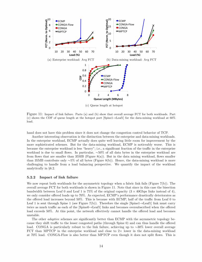
5.2.2 Impact of link failure

We now repeat both workloads for the asymmetric topology when a fabric link fails (Figure 7(b)). Theoverall average FCT for both workloads is shown in Figure 11. Note that since in this case the bisectionbandwidth between Leaf 0 and Leaf 1 is 75% of the original capacity (3 × 40Gbps links instead of 4),we only consider offered loads up to 70%. As expected, ECMP’s performance drastically deteriorates asthe offered load increases beyond 50%. This is because with ECMP, half of the traffic from Leaf 0 toLeaf 1 is sent through Spine 1 (see Figure 7(b)). Therefore the single [Spine1→Leaf1] link must carrytwice as much traffic as each of the [Spine0→Leaf1] links and becomes oversubscribed when the offeredload exceeds 50%. At this point, the network effectively cannot handle the offered load and becomesunstable.

The other adaptive schemes are significantly better than ECMP with the asymmetric topology be-cause they shift traffic to the lesser congested paths (through Spine 0) and can thus handle the offeredload. CONGA is particularly robust to the link failure, achieving up to ∼30% lower overall averageFCT than MPTCP in the enterprise workload and close to 2× lower in the data-mining workloadat 70% load. CONGA-Flow is also better than MPTCP even though it does not split flows. This is

14

0  0.2  0.4  0.6  0.8  1  

0   50   100   150   200  

CDF  

Throughput  Imbalance  (MAX  –  MIN)/AVG  (%)  

ECMP  CONGA-­‐Flow  CONGA  MPTCP  

(a) Enterprise workload

0  0.2  0.4  0.6  0.8  1  

0   50   100   150   200  

CDF  

Throughput  Imbalance  (MAX  –  MIN)/AVG  (%)  

ECMP  CONGA-­‐Flow  CONGA  MPTCP  

(b) Data-mining workload

Figure 12: Extent of imbalance between throughput of leaf uplinks for both workloads at 60% load. Thethroughput samples are over 10ms intervals.

because CONGA proactively detects high utilization paths before congestion occurs and adjusts trafficaccordingly, whereas MPTCP is reactive and only makes adjustments when sub-flows on congested pathsexperience packet drops. This is evident from Figure 11(c), which compares the queue occupancy at thehotspot port [Spine1→Leaf1] for the different schemes for the data-mining workload at 60% load. Wesee that CONGA controls the queue occupancy at the hotspot much more effectively than MPTCP, forinstance, achieving a 4× smaller 90th percentile queue occupancy.

5.2.3 Load balancing efficiency

The FCT results of the previous section show end-to-end performance which is impacted by a varietyof factors, including load balancing. We now focus specifically on CONGA’s load balancing efficiency.Figure 12 shows the CDF of the throughput imbalance across the 4 uplinks at Leaf 0 in the baselinetopology (without link failure) for both workloads at the 60% load level. The throughput imbalance isdefined as the maximum throughput (among the 4 uplinks) minus the minimum divided by the average:(MAX −MIN)/AV G. This is calculated from synchronous samples of the throughput of the 4 uplinksover 10ms intervals, measured using a special debugging module in the ASIC.

The results confirm that CONGA is at least as efficient as MPTCP for load balancing (without anyTCP modifications) and is significantly better than ECMP. CONGA’s throughput imbalance is evenlower than MPTCP for the enterprise workload. With CONGA-Flow, the throughput imbalance isslightly better than MPTCP in the enterprise workload, but worse in the data-mining workload.

5.3 Incast

Our results in the previous section suggest that MPTCP increases congestion at the edge links becauseit opens 8 sub-flows per connection. We now dig deeper into this issue for Incast traffic patterns thatare common in datacenters [3].

We use a simple application that generates the standard Incast traffic pattern considered in priorwork [46, 11, 3]. A client process residing on one of the servers repeatedly makes requests for a 10MBfile striped across N other servers. The servers each respond with 10MB/N of data in a synchronizedfashion causing Incast. We measure the effective throughput at the client for different “fan-in” values,N , ranging from 1 to 63. Note that this experiment does not stress the fabric load balancing since thetotal traffic crossing the fabric is limited by the client’s 10Gbps access link. The performance here ispredominantly determined by the Incast behavior for the TCP or MPTCP transports.

The results are shown in Figure 13. We consider two minimum retransmission timeout (minRTO)values: 200ms (the default value in Linux) and 1ms (recommended by Vasudevan et al. [46] to cope withIncast); and two packet sizes (MTU): 1500B (the standard Ethernet frame size) and 9000B (jumboframes). The plots confirm that MPTCP significantly degrades performance in Incast scenarios. Forinstance, with minRTO = 200ms, MPTCP’s throughput degrades to less than 30% for large fan-in with1500B packets and just 5% with 9000B packets. Reducing minRTO to 1ms mitigates the problem tosome extent with standard packets, but even reducing minRTO does not prevent significant throughputloss with jumbo frames. CONGA +TCP achieves 2–8× better throughput than MPTCP in similarsettings.

15

MTU  1500  

0  20  40  60  80  100  

0   10   20   30   40   50   60  

Throughp

ut  (%

)  

Fanout  (#  of  senders)  

CONGA+TCP  (200ms)  CONGA+TCP  (1ms)  MPTCP  (200ms)  MPTCP  (1ms)  

(a) MTU = 1500B

MTU  9000  

0  20  40  60  80  100  

0   10   20   30   40   50   60  

Throughp

ut  (%

)  

Fanout  (#  of  senders)  

CONGA+TCP  (200ms)  CONGA+TCP  (1ms)  MPTCP  (200ms)  MPTCP  (1ms)  

(b) MTU = 9000B

Figure 13: MPTCP significantly degrades performance in Incast scenarios, especially with large packet sizes(MTU).

Symmetric  Topology  

0  200  400  600  800  1000  

0   5   10   15   20   25   30   35   40  

Comp.  Tim

e  (sec)  

Trial  Number  

ECMP   CONGA   MPTCP  

(a) Baseline Topology (w/o link failure)

Asymmetric  Topology  

0  200  400  600  800  1000  

0   5   10   15   20   25   30   35   40  

Comp.  Tim

e  (sec)  

Trial  Number  

ECMP   CONGA   MPTCP  

(b) Asymmetric Topology (with link failure)

Figure 14: HDFS IO benchmark.

5.4 HDFS Benchmark

Our final testbed experiment evaluates the end-to-end impact of CONGA on a real application. Weset up a 64 node Hadoop cluster (Cloudera distribution hadoop-0.20.2-cdh3u5) with 1 NameNode and63 DataNodes and run the standard TestDFSIO benchmark included in the Apache Hadoop distribu-tion [18]. The benchmark tests the overall IO performance of the cluster by spawning a MapReducejob which writes a 1TB file into HDFS (with 3-way replication) and measuring the total job completiontime. We run the benchmark 40 times for both of the topologies in Figure 7 (with and without link fail-ure). We found in our experiments that the TestDFSIO benchmark is disk-bound in our setup and doesnot produce enough traffic on its own to stress the network. Therefore, in the absence of servers withmore or faster disks, we also generate some background traffic using the empirical enterprise workloaddescribed in §5.2.

Figure 14 shows the job completion times for all trials. We find that for the baseline topology(without failures), ECMP and CONGA have nearly identical performance. MPTCP has some outliertrials with much higher job completion times. For the asymmetric topology with link failure, the jobcompletion times for ECMP are nearly twice as large as without the link failure. But CONGA is robust;comparing Figures 14 (a) and (b) shows that the link failure has almost no impact on the job completiontimes with CONGA. The performance with MPTCP is very volatile with the link failure. Though wecannot ascertain the exact root cause of this, we believe it is because of MPTCP’s difficulties with Incastsince the TestDFSIO benchmark creates a large number of concurrent transfers between the servers.

5.5 Large-Scale Simulations

Our experimental results were for a comparatively small topology (64 servers, 4 switches), 10Gbpsaccess links, one link failure, and 2:1 oversubscription. But in developing CONGA, we also did extensivepacket-level simulations, including exploring CONGA’s parameter space (§3.6), different workloads,larger topologies, varying oversubscription ratios and link speeds, and varying degrees of asymmetry.We briefly summarize our main findings.

Note: We used OMNET++ [45] and the Network Simulation Cradle [23] to port the actual Linux

16

0  

0.2  

0.4  

0.6  

0.8  

1  

30   40   50   60   70   80  FCT  (Normalized

 to  ECM

P)  

Load  (%)  

ECMP  CONGA  

(a) 10Gbps access links

0  

0.2  

0.4  

0.6  

0.8  

1  

30   40   50   60   70   80  FCT  (Normalized

 to  ECM

P)  

Load  (%)  

ECMP  CONGA  

(b) 40Gbps access links

Figure 15: Overall average FCT for a simulated workload based on web search [3] for two topologies with40Gbps fabric links, 3:1 oversubscription, and: (a) 384 10Gbps servers, (b) 96 40Gbps servers.

TCP source code (from kernel 2.6.26) to our simulator. Despite its challenges, we felt that capturingexact TCP behavior was crucial to evaluate CONGA, especially to accurately model flowlets. Since anOMNET++ model of MPTCP is unavailable and we did experimental comparisons, we did not simulateMPTCP.

Varying fabric size and oversubscription: We have simulated realistic datacenter workloads (in-cluding those presented in §5.2) for fabrics with as many as 384 servers, 8 leaf switches, and 12 spineswitches, and for oversubscription ratios ranging from 1:1 to 5:1. We find qualitatively similar results toour testbed experiments at all scales. CONGA achieves ∼5–40% better FCT than ECMP in symmetrictopologies, with the benefit larger for heavy flow size distributions, high load, and high oversubscriptionratios.

Varying link speeds: CONGA’s improvement over ECMP is more pronounced and occurs at lowerload levels the closer the access link speed (at the servers) is to the fabric link speed. For example, intopologies with 40Gbps links everywhere, CONGA achieves 30% better FCT than ECMP even at 30%traffic load, while for topologies with 10Gbps edge and 40Gbps fabric links, the improvement at 30%load is typically 5–10% (Figure 15). This is because in the latter case, each fabric link can supportmultiple (at least 4) flows without congestion. Therefore, the impact of hash collisions in ECMP is lesspronounced in this case (see also [40]).

Varying asymmetry: Across tens of asymmetrical scenarios we simulated (e.g., with different numberof random failures, fabrics with both 10Gbps and 40Gbps links, etc) CONGA achieves near optimaltraffic balance. For example, in the representative scenario shown in Figure 16, the queues at links 10and 12 in the spine (which are adjacent to the failed link 11) are ∼10× larger with ECMP than CONGA.

6 Analysis

In this section we complement our experimental results with analysis of CONGA along two axes. First,we consider a game-theoretic model known as the bottleneck routing game [5] in the context of CONGAto quantify its Price of Anarchy [39]. Next, we consider a stochastic model that gives insights into theimpact of the traffic distribution and flowlets on load balancing performance.

6.1 The Price of Anarchy for CONGA

In CONGA, the leaf switches make independent load balancing decisions to minimize the congestionfor their own traffic. This uncoordinated or “selfish” behavior can potentially cause inefficiency incomparison to having centralized coordination. This inefficiency is known as the Price of Anarchy(PoA) [39] and has been the subject of numerous studies in the theoretical literature (see [42] for asurvey). In this section we analyze the PoA for CONGA using the bottleneck routing game modelintroduced by Banner et al. [5].

Model: We consider a two-tier Leaf-Spine network modeled as a bipartite graph G = (V,E). The leafand spine nodes are connected with links of arbitrary capacities {ce}. The network is shared by a set of

17

0  50  

100  150  200  250  300  

1   11   21   31   41   51   61   71  

Length  (p

kts)  

Link  #  

ECMP  CONGA  

Spine Downlink Queues

0  50  

100  150  200  250  300  

1   11   21   31   41   51   61   71  

Length  (p

kts)  

Link  #  

ECMP  CONGA  

Leaf Uplink Queues

some failed links

some failed links

Figure 16: Multiple link failure scenario in a 288-port fabric with 6 leaves and 4 spines. Each leaf and spineconnect with 3× 40Gbps links and 9 randomly chosen links fail. The plots show the average queue length at allfabric ports for a web search workload at 60% load. CONGA balances traffic significantly better than ECMP.Note that the improvement over ECMP is much larger at the (remote) spine downlinks because ECMP spreadsload equally on the leaf uplinks.

users U . Each user u ∈ U has a traffic demand γu, to be sent from source leaf, su, to destination leaf,tu. A user must decide how to split its traffic along the paths P (su,tu) through the different spine nodes.Denote by fup the flow of user u on path p. The set of all user flows, f = {fup }, is termed the networkflow. A network flow is feasible if

∑p∈P (su,tu) fup = γu for all u ∈ U . Let fp =

∑u∈U f

up be the total flow

on a path and fe =∑p|e∈p fp be the total flow on a link. Also, let ρe(fe) = fe/ce be the utilization of

link e. We define the network bottleneck for a network flow to be the utilization of the most congestedlink; i.e., B(f) , maxe∈E ρe(fe). Similarly, we define the bottleneck for user u to be the utilization ofthe most congested link it uses; i.e., bu(f) , maxe∈E|fue >0 ρe(fe).

We model CONGA as a non-cooperative game where each user selfishly routes its traffic to minimizeits own bottleneck; i.e., it only sends traffic along the paths with the smallest bottleneck available toit. The network flow, f , is said to be at Nash equilibrium if no user can improve its bottleneck giventhe choices of the other users. Specifically, f is a Nash flow if for each user u∗ ∈ U and network flowg = {gup} such that gup = fup for each u ∈ U\u∗, we have: bu∗(f) ≤ bu∗(g). The game above alwaysadmits at least one Nash flow (Theorem 1 in [5]). Note that CONGA converges to a Nash flow becausethe algorithm rebalances traffic (between a particular source/destination leaf) if there is a path with asmaller bottleneck available.4 The PoA is defined as the worst-case ratio of the network bottleneck for aNash flow and the minimum network bottleneck achievable by any flow. We have the following theorem.

Theorem 1. The PoA for the CONGA game is 2.

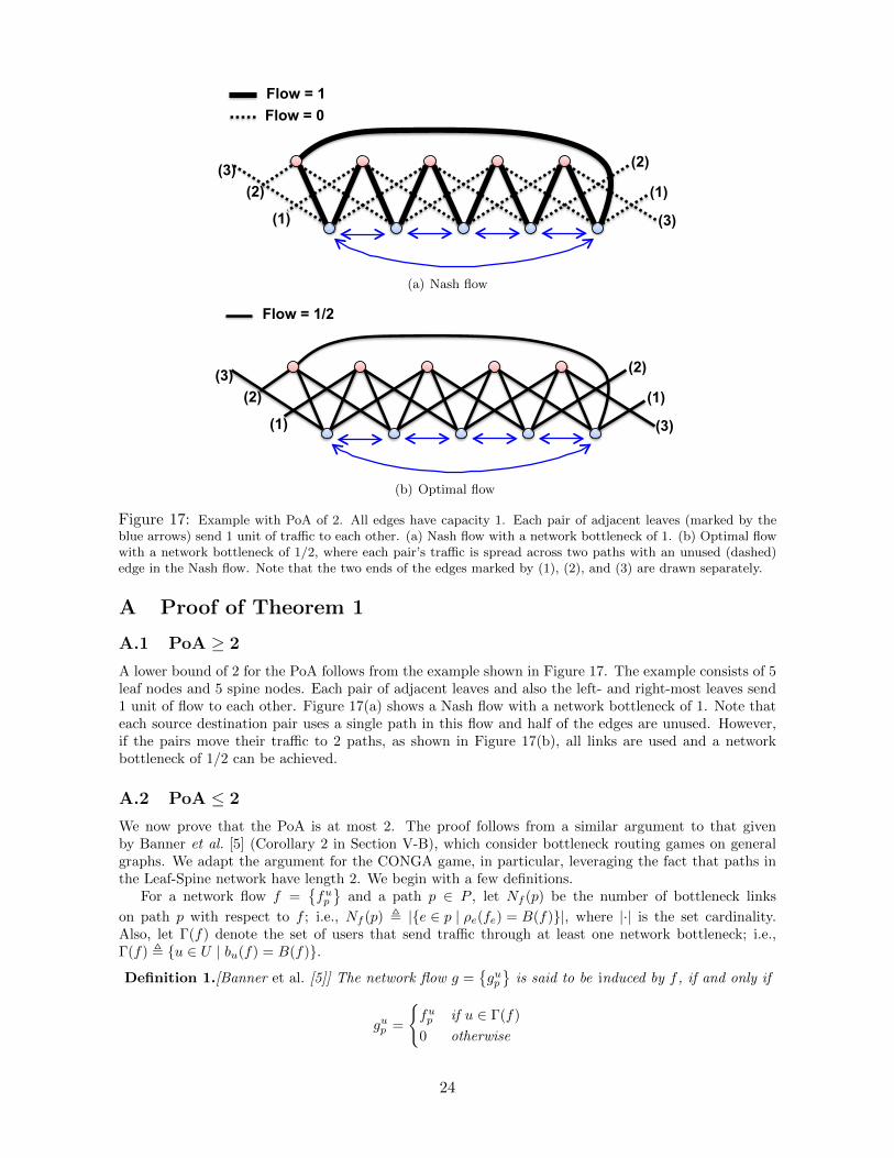
The proof is given in Appendix A. Theorem 1 proves that the network bottleneck with CONGA isat most twice the optimal. It is important to note that this is the worst-case and can only occur invery specific (and artificial) scenarios such as the example in Figure 17. As our experimental evaluationshows (§5), in practice the performance of CONGA is much closer to optimal.

Remark 2. If in addition to using paths with the smallest congestion metric, if the leaf switches alsouse only paths with the fewest number of bottlenecks, then the PoA would be 1 [5], i.e., optimal. Forexample, the flow in Figure 17(a) does not satisfy this condition since traffic is routed along paths withtwo bottlenecks even though alternate paths with a single bottleneck exist. Incorporating this criteriainto CONGA would require additional bits to track the number of bottlenecks along the packet’s path.Since our evaluation (§5) has not shown much potential gains, we have not added this refinement to ourimplementation.

4Of course, this is an idealization and ignores artifacts such as flowlets, quantized congestion metrics, etc.

18

6.2 Impact of Workload on Load Balancing

Our evaluation showed that for some workloads ECMP actually performs quite well and the benefits ofmore sophisticated schemes (such as MPTCP and CONGA) are limited in symmetric topologies. Thisraises the question: How does the workload affect load balancing performance? Importantly, when areflowlets helpful?

We now study these questions using a simple stochastic model. Flows with an arbitrary size distri-bution, S, arrive according to a Poisson process of rate λ and are spread across n links. For each flow,a random link is chosen. Let Nk(t) and Ak(t) respectively denote the number of flows and the total

amount of traffic sent on link k in time interval (0, t); i.e., Ak(t) =∑Nk(t)i=1 ski , where ski is the size of

the ith flow assigned to link k. Let Y (t) = min1≤k≤nAk(t) and Z(t) = max1≤k≤nA

k(t) and define thetraffic imbalance:

χ(t) ,Z(t)−W (t)

λE(S)n t

.

This is basically the deviation between the traffic on the maximum and minimum loaded links normalizedby the expected traffic on each link. The following theorem bounds the expected traffic imbalance attime t.

Theorem 2. Assume E(eθS) <∞ in a neighborhood of zero: θ ∈ (−θ0, θ0). Then for t sufficiently large:

E(χ(t)) ≤ 1√λet

+O(1

t), (1)

where:

λe =λ

8n log n(

1 + ( σSE(S) )2

) . (2)

Here σS is the standard deviation of S.

Note: Kandula et al. [26] prove a similar result for the deviation of traffic on a single link from itsexpectation while Theorem 2 bounds the traffic imbalance across all links.

The proof follows standard probabilistic arguments and is given in Appendix B. Theorem 2 showsthat the traffic imbalance with randomized load balancing vanishes like 1/

√t for large t. Moreover,

the leading term is determined by the effective arrival rate, λe, that depends on two factors: (i) theper-link flow arrival rate, λ/n; and (ii) the coefficient of variation of the flow size distribution, σS/E(S).Theorem 2 quantifies the intuition that workloads that consists mostly of small flows are easier tohandle than workloads with a few large flows. Indeed, it is for the latter “heavy” workloads that we cananticipate flowlets to make a difference. This is consistent with our experiments which show that ECMPdoes well for the enterprise workload (Figure 9), but for the heavier data mining workload CONGA ismuch better than ECMP and is even notably better than CONGA-Flow (Figure 10).

7 Discussion

We make a few remarks on aspects not covered thus far.

Incremental deployment: An interesting consequence of CONGA’s resilience to asymmetry is that itdoes not need to be applied to all traffic. Traffic that is not controlled by CONGA simply creates band-width asymmetry to which (like topology asymmetry) CONGA can adapt. This facilitates incrementaldeployment since some leaf switches can use ECMP or any other scheme. Regardless, CONGA reducesfabric congestion to the benefit of all traffic.

Larger topologies: While 2-tier Leaf-Spine topologies suffice for most enterprise deployments, thelargest mega datacenters require networks with 3 or more tiers. CONGA may not achieve the optimaltraffic balance in such cases since it only controls the load balancing decision at the leaf switches (recallthat the spine switches use ECMP). However, large datacenter networks are typically organized asmultiple pods, each of which is a 2-tier Clos [1, 17]. Therefore, CONGA is beneficial even in these casessince it balances the traffic within each pod optimally, which also reduces congestion for inter-pod traffic.Moreover, even for inter-pod traffic, CONGA makes better decisions than ECMP at the first-hop.

19

A possible approach to generalizing CONGA to larger topologies is to pick a sufficient number of“good” paths between each pair of leaf switches and use leaf-to-leaf feedback to balance traffic acrossthem. While we cannot cover all paths in general (as we do in the 2-tier case), the theoretical literaturesuggests that simple path selection policies such as periodically sampling a random path and retainingthe best paths may perform very well [29]. We leave to future work a full exploration of CONGA inlarger topologies.

Other path metrics: We used the max of the link congestion metrics as the path metric, but of courseother choices such as the sum of link metrics are also possible and can easily be incorporated in CONGA.Indeed, in theory, the sum metric gives a Price of Anarchy (PoA) of 4/3 in arbitrary topologies [42].Of course, the PoA is for the worst-case (adversarial) scenario. Hence, while the PoA is better for thesum metric than the max, like prior work (e.g., TeXCP [25]), we used max because it emphasizes thebottleneck link and is also easier to implement; the sum metric requires extra bits in the packet headerto prevent overflow when doing additions.

8 Related Work

We briefly discuss related work that has informed and inspired our design, especially work not previouslydiscussed.

Traditional traffic engineering mechanisms for wide-area networks [14, 13, 41, 48] use centralizedalgorithms operating at coarse timescales (hours) based on long-term estimates of traffic matrices. Morerecently, B4 [22] and SWAN [20] have shown near optimal traffic engineering for inter-datacenter WANs.These systems leverage the relative predictability of WAN traffic (operating over minutes) and are notdesigned for highly volatile datacenter networks. CONGA is conceptually similar to TeXCP [25] whichdynamically load balances traffic between ingress-egress routers (in a wide-area network) based on path-wise congestion metrics. CONGA however is significantly simpler (while also being near optimal) sothat it can be implemented directly in switch hardware and operate at microsecond time-scales, unlikeTeXCP which is designed to be implemented in router software.

Besides Hedera [2], work such as MicroTE [8] proposes centralized load balancing for datacenters andhas the same issues with handling traffic volatility. F10 [33] also uses a centralized scheduler, but usesa novel network topology to optimize failure recovery, not load balancing. The Incast issues we pointout for MPTCP [40] can potentially be mitigated by additional mechanisms such as explicit congestionsignals (e.g., XMP [10]), but complex transports are challenging to validate and deploy in practice.

A number of papers target the coarse granularity of flow-based balancing in ECMP. Besides Flare [26],LocalFlow [43] proposes spatial flow splitting based on TCP sequence numbers and DRB [9] proposesefficient per-packet round-robin load balancing. As explained in §2.4, such local schemes may interactpoorly with TCP in the presence of asymmetry and perform worse than ECMP. DeTail [51] proposesa per-packet adaptive routing scheme that handles asymmetry using layer-2 back-pressure, but requiresend-host modifications to deal with packet reordering.

9 Conclusion

The main thesis of this paper is that datacenter load balancing is best done in the network instead ofthe transport layer, and requires global congestion-awareness to handle asymmetry. Through exten-sive evaluation with a real testbed, we demonstrate that CONGA provides better performance thanMPTCP [40], the state-of-the-art multipath transport for datacenter load balancing, without importantdrawbacks such as complexity and rigidity at the transport layer and poor Incast performance. Further,unlike local schemes such as ECMP and Flare [26], CONGA seamlessly handles asymmetries in thetopology or network traffic. CONGA’s resilience to asymmetry also paid unexpected dividends whenit came to incremental deployment. Even if some switches within the fabric use ECMP (or any othermechanism), CONGA’s traffic can work around bandwidth asymmetries and benefit all traffic.

CONGA leverages an existing datacenter overlay to implement a leaf-to-leaf feedback loop and canbe deployed without any modifications to the TCP stack. While leaf-to-leaf feedback is not always thebest strategy, it is near-optimal for 2-tier Leaf-Spine fabrics that suffice for the vast majority of deployed

20

datacenters. It is also simple enough to implement in hardware as proven by our implementation incustom silicon.

In summary, CONGA senses the distant drumbeats of remote congestion and orchestrates flowlets todisperse evenly through the fabric. We leave to future work the task of designing more intricate rhythmsfor more general topologies.

Acknowledgments: We are grateful to Georges Akis, Luca Cafiero, Krishna Doddapaneni, Mike Her-bert, Prem Jain, Soni Jiandani, Mario Mazzola, Sameer Merchant, Satyam Sinha, Michael Smith, andPauline Shuen of Insieme Networks for their valuable feedback during the development of CONGA. Wewould also like to thank Vimalkumar Jeyakumar, Peter Newman, Michael Smith, our shepherd TeemuKoponen, and the anonymous SIGCOMM reviewers whose comments helped us improve the paper.

References

[1] M. Al-Fares, A. Loukissas, and A. Vahdat. A scalable, commodity data center network architecture.In SIGCOMM, 2008.

[2] M. Al-Fares, S. Radhakrishnan, B. Raghavan, N. Huang, and A. Vahdat. Hedera: Dynamic FlowScheduling for Data Center Networks. In NSDI, 2010.

[3] M. Alizadeh et al. Data center TCP (DCTCP). In SIGCOMM, 2010.

[4] M. Alizadeh et al. pFabric: Minimal Near-optimal Datacenter Transport. In SIGCOMM, 2013.

[5] R. Banner and A. Orda. Bottleneck Routing Games in Communication Networks. Selected Areasin Communications, IEEE Journal on, 25(6):1173–1179, 2007.

[6] M. Beck and M. Kagan. Performance Evaluation of the RDMA over Ethernet (RoCE) Standard inEnterprise Data Centers Infrastructure. In DC-CaVES, 2011.

[7] T. Benson, A. Akella, and D. A. Maltz. Network Traffic Characteristics of Data Centers in theWild. In SIGCOMM, 2010.

[8] T. Benson, A. Anand, A. Akella, and M. Zhang. MicroTE: Fine Grained Traffic Engineering forData Centers. In CoNEXT, 2011.

[9] J. Cao et al. Per-packet Load-balanced, Low-latency Routing for Clos-based Data Center Networks.In CoNEXT, 2013.

[10] Y. Cao, M. Xu, X. Fu, and E. Dong. Explicit Multipath Congestion Control for Data CenterNetworks. In CoNEXT, 2013.

[11] Y. Chen, R. Griffith, J. Liu, R. H. Katz, and A. D. Joseph. Understanding TCP Incast ThroughputCollapse in Datacenter Networks. In WREN, 2009.

[12] N. Dukkipati and N. McKeown. Why Flow-completion Time is the Right Metric for CongestionControl. SIGCOMM Comput. Commun. Rev., 2006.

[13] A. Elwalid, C. Jin, S. Low, and I. Widjaja. MATE: MPLS adaptive traffic engineering. In INFO-COM, 2001.

[14] B. Fortz and M. Thorup. Internet traffic engineering by optimizing OSPF weights. In INFOCOM,2000.

[15] R. Gallager. A Minimum Delay Routing Algorithm Using Distributed Computation. Communica-tions, IEEE Transactions on, 1977.

[16] P. Gill, N. Jain, and N. Nagappan. Understanding Network Failures in Data Centers: Measurement,Analysis, and Implications. In SIGCOMM, 2011.

[17] A. Greenberg et al. VL2: a scalable and flexible data center network. In SIGCOMM, 2009.

[18] Apache Hadoop. http://hadoop.apache.org/.

[19] C.-Y. Hong, M. Caesar, and P. B. Godfrey. Finishing Flows Quickly with Preemptive Scheduling.In SIGCOMM, 2012.

[20] C.-Y. Hong et al. Achieving High Utilization with Software-driven WAN. In SIGCOMM, 2013.

21

[21] R. Jain and S. Paul. Network virtualization and software defined networking for cloud computing:a survey. Communications Magazine, IEEE, 51(11):24–31, 2013.

[22] S. Jain et al. B4: Experience with a Globally-deployed Software Defined Wan. In SIGCOMM,2013.

[23] S. Jansen and A. McGregor. Performance, Validation and Testing with the Network SimulationCradle. In MASCOTS, 2006.

[24] V. Jeyakumar et al. EyeQ: Practical Network Performance Isolation at the Edge. In NSDI, 2013.

[25] S. Kandula, D. Katabi, B. Davie, and A. Charny. Walking the Tightrope: Responsive Yet StableTraffic Engineering. In SIGCOMM, 2005.

[26] S. Kandula, D. Katabi, S. Sinha, and A. Berger. Dynamic Load Balancing Without Packet Re-ordering. SIGCOMM Comput. Commun. Rev., 37(2):51–62, Mar. 2007.

[27] S. Kandula, S. Sengupta, A. Greenberg, P. Patel, and R. Chaiken. The nature of data center traffic:measurements & analysis. In IMC, 2009.

[28] R. Kapoor et al. Bullet Trains: A Study of NIC Burst Behavior at Microsecond Timescales. InCoNEXT, 2013.

[29] P. Key, L. Massoulie, and D. Towsley. Path Selection and Multipath Congestion Control. Commun.ACM, 54(1):109–116, Jan. 2011.

[30] A. Khanna and J. Zinky. The Revised ARPANET Routing Metric. In SIGCOMM, 1989.

[31] M. Kodialam, T. V. Lakshman, J. B. Orlin, and S. Sengupta. Oblivious Routing of Highly VariableTraffic in Service Overlays and IP Backbones. IEEE/ACM Trans. Netw., 17(2):459–472, Apr. 2009.

[32] T. Koponen et al. Network Virtualization in Multi-tenant Datacenters. In NSDI, 2014.

[33] V. Liu, D. Halperin, A. Krishnamurthy, and T. Anderson. F10: A Fault-tolerant EngineeredNetwork. In NSDI, 2013.

[34] M. Mahalingam et al. VXLAN: A Framework for Overlaying Virtualized Layer 2 Networks overLayer 3 Networks. http://tools.ietf.org/html/draft-mahalingam-dutt-dcops-vxlan-06,2013.

[35] N. Michael, A. Tang, and D. Xu. Optimal link-state hop-by-hop routing. In ICNP, 2013.

[36] MultiPath TCP - Linux Kernel implementation. http://www.multipath-tcp.org/.

[37] T. Narten et al. Problem Statement: Overlays for Network Virtualization. http://tools.ietf.

org/html/draft-ietf-nvo3-overlay-problem-statement-04, 2013.

[38] J. Ousterhout et al. The case for RAMCloud. Commun. ACM, 54, July 2011.

[39] C. Papadimitriou. Algorithms, Games, and the Internet. In Proc. of STOC, 2001.

[40] C. Raiciu et al. Improving datacenter performance and robustness with multipath tcp. In SIG-COMM, 2011.

[41] M. Roughan, M. Thorup, and Y. Zhang. Traffic engineering with estimated traffic matrices. InIMC, 2003.

[42] T. Roughgarden. Selfish Routing and the Price of Anarchy. The MIT Press, 2005.

[43] S. Sen, D. Shue, S. Ihm, and M. J. Freedman. Scalable, Optimal Flow Routing in Datacenters viaLocal Link Balancing. In CoNEXT, 2013.

[44] M. Sridharan et al. NVGRE: Network Virtualization using Generic Routing Encapsulation. http://tools.ietf.org/html/draft-sridharan-virtualization-nvgre-03, 2013.

[45] A. Varga et al. The OMNeT++ discrete event simulation system. In ESM, 2001.

[46] V. Vasudevan et al. Safe and effective fine-grained TCP retransmissions for datacenter communi-cation. In SIGCOMM, 2009.

[47] S. Vutukury and J. J. Garcia-Luna-Aceves. A Simple Approximation to Minimum-delay Routing.In SIGCOMM, 1999.

[48] H. Wang et al. COPE: Traffic Engineering in Dynamic Networks. In SIGCOMM, 2006.

22

[49] D. Wischik, C. Raiciu, A. Greenhalgh, and M. Handley. Design, Implementation and Evaluationof Congestion Control for Multipath TCP. In NSDI, 2011.

[50] D. Xu, M. Chiang, and J. Rexford. Link-state Routing with Hop-by-hop Forwarding Can AchieveOptimal Traffic Engineering. IEEE/ACM Trans. Netw., 19(6):1717–1730, Dec. 2011.

[51] D. Zats, T. Das, P. Mohan, D. Borthakur, and R. H. Katz. DeTail: Reducing the Flow CompletionTime Tail in Datacenter Networks. In SIGCOMM, 2012.

23

(1)

(1)

(2)

(2) (3)

(3)

Flow = 1 Flow = 0

(a) Nash flow

(1)

(1)

(2)

(2) (3)

(3)

Flow = 1/2

(b) Optimal flow

Figure 17: Example with PoA of 2. All edges have capacity 1. Each pair of adjacent leaves (marked by theblue arrows) send 1 unit of traffic to each other. (a) Nash flow with a network bottleneck of 1. (b) Optimal flowwith a network bottleneck of 1/2, where each pair’s traffic is spread across two paths with an unused (dashed)edge in the Nash flow. Note that the two ends of the edges marked by (1), (2), and (3) are drawn separately.

A Proof of Theorem 1

A.1 PoA ≥ 2

A lower bound of 2 for the PoA follows from the example shown in Figure 17. The example consists of 5leaf nodes and 5 spine nodes. Each pair of adjacent leaves and also the left- and right-most leaves send1 unit of flow to each other. Figure 17(a) shows a Nash flow with a network bottleneck of 1. Note thateach source destination pair uses a single path in this flow and half of the edges are unused. However,if the pairs move their traffic to 2 paths, as shown in Figure 17(b), all links are used and a networkbottleneck of 1/2 can be achieved.

A.2 PoA ≤ 2

We now prove that the PoA is at most 2. The proof follows from a similar argument to that givenby Banner et al. [5] (Corollary 2 in Section V-B), which consider bottleneck routing games on generalgraphs. We adapt the argument for the CONGA game, in particular, leveraging the fact that paths inthe Leaf-Spine network have length 2. We begin with a few definitions.

For a network flow f ={fup}

and a path p ∈ P , let Nf (p) be the number of bottleneck links

on path p with respect to f ; i.e., Nf (p) , |{e ∈ p | ρe(fe) = B(f)}|, where |·| is the set cardinality.Also, let Γ(f) denote the set of users that send traffic through at least one network bottleneck; i.e.,Γ(f) , {u ∈ U | bu(f) = B(f)}.

Definition 1.[Banner et al. [5]] The network flow g ={gup}

is said to be induced by f , if and only if

gup =

{fup if u ∈ Γ(f)

0 otherwise

24

Hence, g consists of exactly the traffic for those users in f that use at least one bottleneck.

The following are straightforward consequences of this definition.

Lemma 1. If g is induced by f , then:

1. The network bottleneck of g equals that of f : B(g) = B(f).

2. The set of bottleneck links with respect to f and g are the same.

3. g is feasible for users u ∈ Γ(f);. i.e., it satisfies their demands:∑p∈P (su,tu) gup = γu for all u ∈ Γ(f).

4. If f is a Nash flow for users u ∈ U , then g is a Nash flow for users u ∈ Γ(f).

Proof. See Lemma A.1 and Lemma 4 in [5].

Consider an arbitrary Nash flow f of the CONGA game. We wish to show that the network bottleneckof f is within a factor of 2 of the optimal network bottleneck. The following lemma states that it issufficient to prove this for the flow g induced by f .

Lemma 2. Let g be induced by a Nash flow f . If B(g) ≤ 2B(g∗), then B(f) ≤ 2B(f∗), where g∗ and f∗

are the optimal flows (that minimize the network bottleneck) among all feasible flows for users in Γ(f)and U respectively.

Proof. Using Lemma 1, B(g) = B(f). Also, B(g∗) ≤ B(f∗) because f∗ must satisfy the demands of allusers that g∗ satisfies (and possibly more). Hence,

B(f) = B(g) ≤ 2B(g∗) ≤ 2B(f∗),

which completes the proof.

Henceforth, we restrict our attention to g. Assume there exists a network flow h which satisfies thedemands of users u ∈ Γ(f) (and only those users), and for which B(g) > 2B(h). We will show that thisis not possible by contradiction, thereby proving the upper bound of 2 on the PoA for f using Lemma 2.

Let E be the set of links that are bottlenecks with respect to g; i.e., E = {e ∈ E | ρe(ge) = B(g)}.Also, let P (e) denote the set of all paths that traverse a link e. Since B(g) > 2B(h), it follows thatρe(ge) > 2ρe(he) for each e ∈ E, and consequently that ge > 2he for each e ∈ E (recall that ρe(x) =x/ce). Thus, for each e ∈ E, ∑

p∈P (e)

gp > 2∑

p∈P (e)

hp.

Summing these inequalities for all e ∈ E, we have∑e∈E

∑p∈P (e)

gp > 2∑e∈E

∑p∈P (e)

hp. (3)

Now let P ,⋃e∈E

P (e) be the set of all paths that traverse a bottleneck link in E. Equation (3) can be

rewritten as ∑p∈P

gpNg(p) > 2∑p∈P

hpNg(p).

Recall that Ng(p) is the number of bottleneck links on path p with respect to g. Using the fact thatNg(p) ≤ 2 for any all p (because the paths in a Leaf-Spine network have length 2), and that Ng(p) ≥ 1for p ∈ P , we have

2∑p∈P

gp ≥∑p∈P

gpNg(p) > 2∑p∈P

hpNg(p) ≥ 2∑p∈P

hp,

and therefore ∑p∈P

gp >∑p∈P

hp. (4)

In the rest of the proof, we proceed to show that Equation (4) contradicts the feasibility of both gand h for users in Γ(f). Define Q ,

⋃u∈Γ(f) P

(su,tu) as the set of all paths for users u ∈ Γ(f). Note

25

that Q ⊆ P . This is because each path p ∈ P (su,tu) for a user u ∈ Γ(f) must traverse at least onebottleneck link in E; otherwise, u could reduce its bottleneck by shifting some of its traffic to the pathp, contradicting the fact that g is a Nash flow (Lemma 1). Further, since the network flows g and h onlycontain traffic from users u ∈ Γ(f), we have∑

p∈P\Q

gp =∑

p∈P\Q

hp = 0.

This combined with Equation (4) gives ∑p∈Q

gp >∑p∈Q

hp,

which is equivalent to ∑u∈Γ(f)

∑p∈P (su,tu)

gp >∑

u∈Γ(f)

∑p∈P (su,tu)

hp. (5)

But since g and h are feasible for users u ∈ Γ(f), we have∑p∈P (su,tu)

gp =∑

p∈P (su,tu)

hp = γu,

for each u ∈ Γ(f). This contradicts Equation (5).

B Proof of Theorem 2

Let Z(t) = max1≤k≤nAk(t). For any θ ∈ (0, θ0), we have

eθE(Z(t))(a)

≤ E(eθZ(t)

)= E

(max

1≤k≤neθA

k(t)

)≤

n∑k=1

E(eθA

k(t))

(b)= nE

(eθA

1(t)). (6)

Here, (a) results from Jensen’s inequality and (b) is true because the random variables Ak(t) are iden-tically distributed. Let MS(θ) = E

(eθS)

be the moment generating function of S. Note that MS(θ)exists for θ ∈ (−θ0, θ0). We have:

E(eθA

1(t))

= E

exp

θN1(t)∑i=1

S1i

(a)=

∞∑k=0

e−λtn

(λtn

)kk!

E

(exp

{θ

k∑i=1

S1i

}∣∣∣∣∣ N1(t) = k

)(b)=

∞∑k=0

e−λtn

(λtn

)kk!

E

(exp

{θ

k∑i=1

S1i

})(c)=

∞∑k=0

e−λtn

(λtn

)kk!

E(eθS)k

= eλtn (MS(θ)−1). (7)

In the above, (a) follows because N1(t) is Poisson with mean λtn ; (b) follows because N1(t) and {S1

i }are independent; and (c) follows because {S1

i } are i.i.d. random variables. Equations (6) and (7) give

eθE(Z(t)) ≤ neλtn (MS(θ)−1)

for θ ∈ (0, θ0). Therefore,

E (Z(t)) ≤ log n

θ+λt

n

(MS(θ)− 1

θ

),

26

and plugging in the Taylor series expansion,

MS(θ) = 1 + E(S)θ +1

2E(S2)θ2 +O(θ3),

we obtain

E (Z(t)) ≤ λtE(S)

n+

log n

θ+λtE(S2)

2nθ +

λt

nO(θ2), (8)

for θ ∈ (0, θ0). Let θ∗ =√

2n lognλE(S2)t . Note that θ∗ ∈ (0, θ0) for t > 2n logn

λE(S2)θ20. Setting θ = θ∗ in Equation (8)

yields

E (Z(t)) ≤ λE(S)

nt+

√2λE (S2) log n

nt+O(1). (9)

A nearly identical argument for W (t) = min1≤k≤nAk(t) gives

E (W (t)) ≥ λE(S)

nt−√

2λE (S2) log n

nt+O(1), (10)

for t > 2n lognλE(S2)θ20

. Equations (9) and (10), along with the fact that E (W (t)) ≤ E (Z(t)), give

E (χ(t)) =E (Z(t))− E (W (t))

λE(S)n t

≤

√8n log nE (S2)

λE (S)2t

+O(1

t), (11)

which is the same as Equation (1).

27