conditions for robustness to nonnormality of … for robustness to nonnormality of test statistics...
TRANSCRIPT
Conditions for Robustness to Nonnormality
of Test Statistics in a GMANOVA Model
Hirokazu Yanagihara
Department of Social Systems and Management
Graduate School of Systems and Information Engineering
University of Tsukuba
1-1-1 Tennodai, Tsukuba, Ibaraki 305-8573, Japan
E-mail : [email protected]
(Last Modified: February 27, 2006)
Abstract
This paper discusses the conditions for robustness to the nonnormality of
three test statistics for a general multivariate linear hypothesis, which were
proposed under the normal assumption in a generalized multivariate analysis
of variance (GMANOVA) model. Although generally the second terms in the
asymptotic expansions of the mean and variance of the test statistics consist
of skewness and kurtosis of an unknown population’s distribution, we find
conditions where the skewness and kurtosis disappear from the second term
in the asymptotic expansions under any distributions. When such conditions
are satisfied, the Bartlett correction and the modified Bartlett correction in
the normal case improve the chi-square approximation even under nonnor-
mality. By using these conditions, it is possible to see whether the used test
statistic is robust to nonnormality or not.
AMS 2000 subject classifications. Primary 62F05; Secondary 62F35.
Key words: Actual test size; Asymptotic expansion; Bartlett correction;
Chi-square approximation; General multivariate linear hypothesis; Modified
Bartlett correction; Nominal test size; Null distribution; Robust design.
1
1. Introduction
Over the past few decades, many authors have investigated the influ-
ences of nonnormality in several statistical test procedures proposed under
the normal assumption, and we have been able to obtain many results from
these studies. For the test size (or the significant level), it is well known that
Hotelling’s two-sample test is robust to nonnormality and Hotelling’s one-
sample test is not. Chase and Bulge (1971), and Everett (1979) obtained
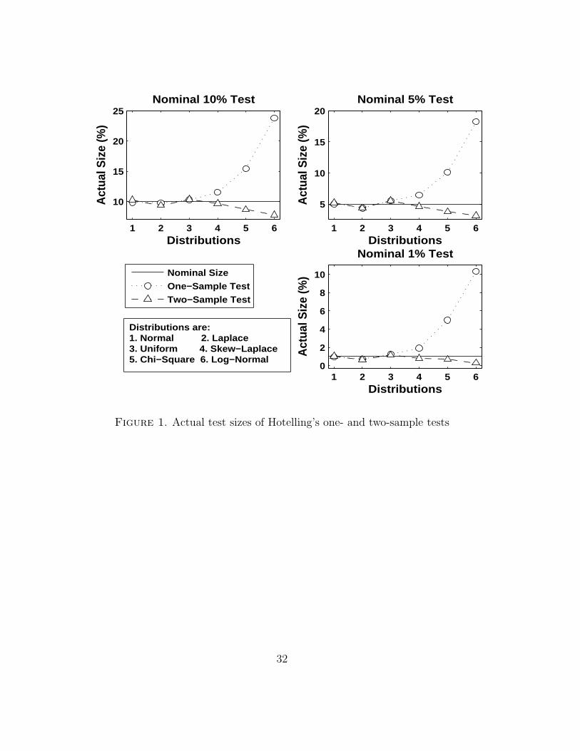
this fact through numerical experiments. Figure 1 shows the numerical re-
sults of actual test sizes of the two test statistics in the case of sample size
n = 20 and the dimension of observation p = 2 when we use six distribu-
tions as the population distributions (i.e., the true distributions). The six
distributions used are normal, Laplace, uniform, skew-Laplace, chi-square
and log-normal distributions (for details of the setting of true distributions
in numerical studies, see Appendix A.1). This figure shows actual test sizes
under those true distributions when we believe that the data came from the
normal distribution, i.e., we use the F -distribution as the null distribution.
From this figure, we can say that the difference of the actual test sizes of the
two-sample test by the difference in distributions is small, but the one-sample
test is not. In the case of the one-sample test, as the skewness of the true
distributions becomes large, the differences between the actual and nominal
test sizes grow. If the 10% test size becomes the 15 % or 25 % test size,
which we believe happens, we cannot say that this will be used.
Insert Figure 1 around here
There is a large difference in the influence of nonnormality of two test
statistics; however, the statistical model in both tests is essentially a mul-
tivariate linear model. What is the difference between these two? In this
paper, we give the theoretical answer for this question, but not the numer-
ical answer, which has not yet been obtained. There is a serious difference
2
between the two tests in the second term of an asymptotic expansion of the
mean of the test statistic. Although there are skewnesses of the true distribu-
tion in the second term of such an expansion of the one-sample test statistic,
there is no skewness to that of the one-sample test statistic. In this paper, we
set the test statistic as robust to nonnormality when there are not cumulants
denoting nonnormality in the second term of an asymptotic expansion of its
moments.
We extend the considered test statistic to the test statistic for a general
multivariate linear hypothesis in the generalized multivariate analysis of vari-
ance (GMANOVA) model (Potthoff & Roy, 1964) from Hotelling’s one- and
two-sample test statistics, and search for conditions where the cumulants de-
noting nonnormality of the true distribution disappear from the second term
of an asymptotic expansion of the mean of the test statistic. In addition,
there is a condition where the cumulants disappear from the second term in
an asymptotic expansion of the variance of the test statistic. These condi-
tions are made clearer through the coefficients of an asymptotic expansion
of the null distribution of the test statistic. By using these conditions, it is
possible to see whether or not the used test statistic is robust to nonnormal-
ity. Moreover, when these conditions are satisfied, the Bartlett correction
(Bartlett, 1937) or the modified Bartlett correction (Fujikoshi, 2000) in the
normal case can give an improvement of the chi-square approximation under
any distributions. It is very important to improve the chi-square approxi-
mation without estimating skewnesses and kurtosis, because it is difficult to
obtain good estimators of skewness and kurtosis without an adequate sample
size. Especially, the bias of the ordinary estimator of kurtosis proposed by
Mardia (1970) becomes large unless the sample size is huge (see Yanagihara,
2006).
The present paper is organized as follows. In Section 2, we state asymp-
totic expansions, obtained by Yanagihara (2001), to the null distributions of
the three test statistics in a GMANOVA model. By using the coefficients of
3
these expansions, the conditions under which the test statistics are robust to
nonnormality become clear in Section 3. Then, we confirm that when these
conditions are satisfied, the Bartlett correction and the modified Bartlett
correction in the normal case can give an improvement of the chi-square ap-
proximation under any distributions. We conclude our discussion in Section
4. Technical details are provided in the Appendix.
2. Asymptotic Expansions of Null Distributions
of Test Statistics in the GMANOVA Model
The GMANOVA model proposed by Potthoff and Roy (1964) is defined
by
Y = AΞX ′ + EΣ1/2, (2.1)
where Y = (y1, . . . ,yn)′ is an n×p observation matrix of response variables,
A = (a1, . . . ,an)′ is an n × k between-individuals design matrix of explana-
tory variables with the full rank k (< n), X is a p × q within-individuals
design matrix of explanatory variables with the full rank q (≤ p), Ξ is a k×q
unknown parameter matrix, and E = (ε1, . . . , εn)′ is an n × p unobserved
error matrix. It is assumed that ε1, . . . , εn are independent random vectors
from ε = (ε1, . . . , εp)′, and the true distribution of ε is distributed follow-
ing an unknown distribution with a mean E[ε] = 0p and covariance matrix
Cov[ε] = Ip, where 0p is a p × 1 vector, all of whose elements are 0. This
model can frequently be applied to the analysis of growth curve data, and
therefore it is also called the growth curve model.
We consider testing for a general linear hypothesis as
H0 : CΞD = Oc×d, (2.2)
where C is a known c× k matrix with the rank c (≤ k), D is a known q × d
matrix with the rank d (≤ q), and Oc×d is a c×d matrix, all of whose elements
are 0. Let Sh and Se be the variation matrices due to the hypothesis and
4
the error respectively, i.e.,
Sh = (CΞD)′(CRC ′)−1(CΞD), Se = D′(X ′S−1X)−1D,
where
Ξ = (A′A)−1A′Y S−1X(X ′S−1X)−1,
R = (A′A)−1A′ (In + Y S−1Y ′)A(A′A)−1 − Ξ(X ′S−1X)Ξ′,
and S = Y ′(In − P�)Y . Here, P� is the projection matrix to the linear
space R(A) generated by the column vectors of A, i.e., P� = A(A′A)−1A′.
Then, the three criteria proposed for testing (2.2) under normality, in par-
ticular, are as follows.
(i) the likelihood ratio statistic (LR):TLR = −{n − k − (p − q)} log(|Se|/|Se + Sh|),
(ii) the Lawley-Hotelling trace criterion (HL):THL = {n − k − (p − q)}tr(ShS
−1e ),
(iii) the Bartlett-Nanda-Pillai trace criterion (BNP):TBNP = {n − k − (p − q)}tr {Sh(Sh + Se)
−1} ,
(2.3)
(for these results, see e.g., von Rosen, 1991; Fujikoshi, 1993; Srivastava & von
Rosen, 1999). By changing the known coefficient matrices for hypotheses C
and D, it is possible to express several linear hypotheses. For these examples,
see Kshirsagar and Smith (1995, p. 40) and Yanagihara (2001).
In order to simplify the results of the asymptotic expansions in Yanagi-
hara (2001), we state some notations of the moments and cumulants of the
true distribution, and some projection matrices. Let μi1 ···im be an mth mul-
tivariate moment of ε defined by
μi1 ···im = E[εi1 · · · εim ].
Similarly, the corresponding mth multivariate cumulant of ε is denoted by
κi1···im , e.g.,
κabc = μabc, κabcd = μabcd − δabδcd − δacδbd − δadδbc,
5
where δab is the Kronecker delta, i.e., δaa = 1 and δab = 0 for a �= b. Let e1
and e2 be independent random vectors from ε. We define the multivariate
skewness and kurtosis of the transformed ε by the symmetric p× p matrices
H , L and M , whose (a, b)th elements are hab, lab and mab, respectively, as
κ(H,M) = E�1 [(e′1He1)(e
′1Me1)] − {tr(H)tr(M ) + 2tr(HM )}
=
p∑a,b,c,d
κabcdhabmcd,
γ21(H ,L,M) = E�1E�2
[(e′1He2)(e
′1Le2)(e
′1Me2)]
=
p∑a,b,c,d,e,f
κabcκdefhadlbemcf ,
γ22(H ,L,M) = E�1E�2 [(e′
1He1)(e′1Le2)(e
′2Me2)]
=
p∑a,b,c,d,e,f
κabcκdefhablcdmef ,
where the notation∑p
a1,...,ajmeans
∑pa1=1 · · ·
∑paj=1. Then, the ordinary
multivariate skewnesses and kurtosis (see e.g., Mardia, 1970, and Isogai,
1983) can be expressed as
κ(1)4 = κ(Ip, Ip), κ
(1)3,3 = γ2
1(Ip, Ip, Ip), κ(2)3,3 = γ2
2(Ip, Ip, Ip).
Let an n × n idempotent matrix B whose (i, j)th element is bij be given by
B = A(A′A)−1C ′{C(A′A)−1C ′}−1C(A′A)−1A′.
Then, the matrices B(d) and B(3) are defined by bij as B(d) = diag(b11, . . . , bnn)
and B(3) = [b3ij], which means the (i, j)th element of B(3) is b3
ij. The projec-
tion matrices Ψ and Φ are given by
Ψ = Σ−1/2X(X ′Σ−1X)−1D{D′(X ′Σ−1X)−1D}D′(X ′Σ−1X)−1X ′Σ−1/2,
Φ = Ip −Σ−1/2X(X ′Σ−1X)−1X ′Σ−1/2.
By using these notations, asymptotic expansions of the null distributions of
the test statistics in (2.3), obtained by Yanagihara (2001), are expressed as
in the following lemma.
6
Lemma 2.1. Suppose that the between-individuals design matrix A and the
true distribution of the error matrix E satisfy the following five assumptions:
1. lim supn→∞
1
n
n∑j=1
‖aj‖4 < ∞, where ‖ · ‖ denotes the Euclidean norm.
2. lim infn→∞
λn
n> 0, where λn is the smallest eigenvalue of A′A,
3. For some constant δ ∈ (0, 1/2], Mn = O(n1/2−δ), where Mn = maxj=1,...,n ‖aj‖,
4. E[‖ε‖8] < ∞,
5. The Cramer’s condition for the joint distribution of ε and εε′ holds.
Then, the null distributions of the three test statistics in (2.3) are expanded
as
P(T ≤ x) = Gcd(x) +1
n
3∑j=0
βjGcd+2j(x) + o(n−1), (2.4)
where Gf(x) is the distribution function of the chi-square distribution with f
degrees of freedom, and the coefficients βj are given by
β0 =1
8m
(1)4 κ(Ψ,Ψ) − 1
24
{2m
(1)3,3 + 3(c − 2)(c + 1)m
(1)3,1
}γ2
1 (Ψ,Ψ,Ψ)
−1
8
{m
(2)3,3 − 2m
(1)3,1 − (c − 2)m
(1)1,1
}γ2
2(Ψ,Ψ,Ψ)
−1
2
{2m
(1)3,1 − (2c + 1)m
(1)1,1
}γ2
1(Ψ,Ψ,Φ)
−1
2
{m
(1)3,1 − cm
(1)1,1
}γ2
2(Ψ,Ψ,Φ)
−1
2
{m
(1)3,1 − (c + 1)m
(1)1,1
}γ2
2 (Ψ,Φ,Ψ)
−1
2m
(1)1,1
{3γ2
1(Ψ,Φ,Φ) + 2γ22(Ψ,Φ,Φ) + γ2
2(Φ,Ψ,Φ)}
+1
4cd(c − d − 1),
β1 = −1
4m
(1)4 κ(Ψ,Ψ) +
1
8
{2m
(1)3,3 − 4m
(1)3,1 + (3c2 + c − 6)m
(1)1,1
}γ2
1(Ψ,Ψ,Ψ)
+1
8
{3m
(2)3,3 − 2(3c + 2)m
(1)3,1 + (c + 6)m
(1)1,1
}γ2
2 (Ψ,Ψ,Ψ)
7
+1
2
{4m
(1)3,1 − (4c + 5)m
(1)1,1
}γ2
1(Ψ,Ψ,Φ)
+{
m(1)3,1 − (c + 1)m
(1)1,1
}γ2
2 (Ψ,Ψ,Φ) (2.5)
+1
2{2m(1)
3,1 − (2c + 3)m(1)1,1}γ2
2(Ψ,Φ,Ψ)
+1
2m
(1)1,1{3γ2
1(Ψ,Φ,Φ) + 2γ22(Ψ,Φ,Φ) + γ2
2(Φ,Ψ,Φ)}
−1
2cd{c + r(c + d + 1)},
β2 =1
8m
(1)4 κ(Ψ,Ψ) − 1
8
{2m
(1)3,3 − 8m
(1)3,1 + (c + 2)(3c − 1)m
(1)1,1
}γ2
1 (Ψ,Ψ,Ψ)
−1
8
{3m
(2)3,3 − 6(3c + 4)m
(1)3,1 + 5(c + 2)m
(1)1,1
}γ2
2 (Ψ,Ψ,Ψ)
−{
m(1)3,1 − (c + 2)m
(1)1,1
}γ2
1 (Ψ,Ψ,Φ)
−1
2
{m
(1)3,1 − (c + 2)m
(1)1,1
}{γ2
2 (Ψ,Ψ,Φ) + γ22(Ψ,Φ,Ψ)
}+
1
4cd(c + d + 1)(1 + 2r),
β3 =1
24
{2m
(1)3,3 − 12m
(1)3,1 + 3(c + 1)(c + 2)m
(1)1,1
}γ2
1(Ψ,Ψ,Ψ)
+1
8
{m
(2)3,3 − 2(c + 2)m
(1)3,1 + 3(c + 2)m
(1)1,1
}γ2
2(Ψ,Ψ,Ψ).
Here, the constant r is determined by the test statistics as
r =
⎧⎨⎩
−1/2 (when T is TLR)0 (when T is THL)
−1 (when T is TBNP)
and the coefficients m’s are defined by the between-individuals design matrix
A and the coefficient matrix for hypothesis C as
m(1)1,1 =
1
n1′
nB1n, m(1)4 = ntr
(B2
(d)
)− c(c + 2),
m(1)3,1 = 1′
nB(d)B1n, m(1)3,3 = n1′
nB(3)1n, m(2)3,3 = n1′
nB(d)BB(d)1n,
(2.6)
where 1n is an n × 1 vector, all of whose elements are 1.
8
Notice that
m(1)1,1 =
1
n2
n∑i,j
u′iuj, m
(1)4 =
1
n
n∑i=1
‖ui‖4 − c(c + 2),
m(1)3,1 =
1
n2
n∑i,j
‖ui‖2(u′iuj), m
(1)3,3 =
1
n2
n∑i,j
(u′iuj)
3,
m(2)3,3 =
1
n2
n∑i,j
‖ui‖2‖uj‖2(u′iuj),
(2.7)
where
ui =√
n{C(A′A)−1C ′}−1/2C(A′A)−1ai, (i = 1, . . . , n). (2.8)
Therefore, the coefficients βj (j = 0, 1, 2, 3) are determined by the skewnesses
and kurtosis of ε and sample cumulants of ui (i = 1, . . . , n). From Lemma
2.1, we see that the second term in the asymptotic expansion of the null dis-
tribution of the test statistic in (2.3) depends on the skewnesses and kurtosis
of the true distribution. Therefore, we can generally say that the second
terms in expansions of the mean and variance of the test statistic in (2.3)
consist of the skewnesses and kurtosis of the true distribution. However, in
the next section, we show that there are conditions where the skewnesses and
kurtosis disappear from the second terms of the expansions.
3. Conditions for Robustness to Nonnormality
3.1. Conditions for the mean
In this sub-section, we consider conditions where the cumulants denoting
nonnormality of the true distribution disappear from the second term of an
asymptotic expansion of the mean of the test statistic in (2.3). Notice that∫ ∞
0
xsdGf(x) = f(f + 2) × · · · × (f + 2(s − 1)).
From the formula (2.4) in Lemma 2.1, we obtain an asymptotic expansion of
9
the mean of the test statistic in (2.3) as
E[T ] = cd +1
n
3∑j=0
βj(cd + 2j) + o(n−1).
By using the relation∑3
j=0 βj = 0, we can write a concrete form of the
expansion of the mean as
E[T ] = cd +1
nm
(1)1,1
[γ2
1(Ψ,Ψ,Ψ) + γ22 (Ψ,Ψ,Ψ)
+3{γ2
1(Ψ,Ψ,Φ) + γ21(Ψ,Φ,Φ)
}+2{γ2
2(Ψ,Φ,Ψ) + γ22(Ψ,Φ,Φ)
}+γ2
2(Ψ,Ψ,Φ) + γ22(Φ,Ψ,Φ)
]+
1
ncd {r(c + d + 1) + d + 1} + o(n−1)
= cd(1 +
η1
n
)+ o(n−1). (3.1)
From this equation, we can see that η1 in (3.1) is independent of the cumu-
lants denoting nonnormality if the coefficient m(1)1,1 is 0 or all the γ2
j (∗, ∗, ∗)(j = 1, 2) are 0. It means that a location of the null distribution of the test
statistic is not easily moved due to the nonnormality of the true distribu-
tion. Then, the test statistic becomes robust to nonnormality. Notice that
m(1)1,1 = 0 is equivalent to
1
n1′
nA(A′A)−1C ′{C(A′A)−1C ′}−1C(A′A)−1A′1n = 0.
Since C(A′A)−1C ′ is a positive definite matrix, the above equation can be
rewritten as C(A′A)−1A′1n = 0c. Therefore, we obtain the conditions for
robustness to nonnormality in the following theorem.
Theorem 3.1. If a considered test satisfies either of the following, Condition
1 or 2:
• Condition 1: C(A′A)−1A′1n = 0c,
• Condition 2: All the γ2j (∗, ∗, ∗) (j = 1, 2) are 0,
10
the second term of the asymptotic expansion of the mean of the test statistic
T becomes independent of the cumulants denoting nonnormality of the true
distribution, i.e.,
E[T ] = cd
[1 +
1
n{r(c + d + 1) + d + 1}
]+ o(n−1). (3.2)
Then, the location of the null distribution of T is not easily moved due to
nonnormality of the true distribution.
From Appendix A.2, we can see that all the γ2j (∗, ∗, ∗) are 0 if the true
distribution is an orthant symmetric (Efron, 1969), which is not a skewed
distribution. Therefore, we obtain the following corollary (the proof is given
in Appendix A.2).
Corollary 3.1.If the true distribution is an orthant symmetric, then Con-
dition 2 holds.
It is well known that the elliptical distribution is an orthant symmetric. Many
authors have reported that a test statistic is robust when the distribution of
observation is the elliptical distribution, e.g., Efron (1969), Eaton and Efron
(1970), Dawid (1977), Kariya (1981a, 1981b) and Khartri (1988). Robustness
to nonnormality, which is caused by Condition 2, corresponds to their results.
Although Condition 2 depends on the unknown true distribution, Condi-
tion 1 only depends on the setting of the hypothesis testing. By using Condi-
tion 1, we can judge whether a used test statistic is robust to nonnormality or
not. Moreover, we can consider two types of the between-individuals design
matrix A. When the matrix A has a segment, i.e., A is given by 1n and any
n× (k −1) matrix A+ with the rank k−1 is given as A = (1n A+), then we
call such a design matrix the type I between-individuals design matrix. On
the other hand, when the matrix A is given by
A =
⎛⎜⎝ 1n1
· · · 0n1
.... . .
...0nk
· · · 1nk
⎞⎟⎠ , (3.3)
11
where∑k
i=1 ni = n, then we call such a design matrix the type II between-
individuals design matrix. Through these matrices, we can obtain settings
which satisfy Condition 1 in the following corollary (the proof is given in
Appendix A.3).
Corollary 3.2. We consider the two cases of the between-individuals de-
sign matrix A, i.e., A is type I or type II. Then, Condition 1 holds if the
following conditions of the coefficient matrix for hypothesis C are satisfied.
1. In the case that A is type I, if C = (0c C+), where C+ is any c×(k−1)
matrix with the rank c, Condition 1 holds.
2. In the case that A is type II, if the equation C1k = 0c is satisfied,
Condition 1 holds.
From Corollary 3.2, we can see that Hotelling’s two-sample test satisfies
Condition 1 and Hotelling’s one-sample test does not. Even if the between-
individuals design matrix A is not type I or II, the test can be made to satisfy
Condition 1 through the transformations A → (1n A) and C → (0c C).
Furthermore, we can see that testing for equality, e.g., equality for the means
between k-groups, i.e., H0 : μ1 = · · · = μk, satisfies Condition 1, because
matrix A is type II and C1k = 0c in this case. Practical tests are tests of
the equality for parameters, e.g., the testing equality for several means in a
multi-way MANOVA model; therefore, it seems that our result is useful for
actual use.
If the mean of the test statistic T is expanded as (3.1), then the Bartlett
correction can be obtained as
T =
(1 − η1
n
)T,
where η1 is a consistent estimator of η1. Therefore, in general, it is necessary
to estimate skewnesses in order to use the Bartlett correction. However,
12
from Theorem 3.1, we can see that the Bartlett correction in the normal
case, which is the transformation by the constant coefficient, can improve
a chi-square approximation, even if the true distribution is not the normal
distribution; this is because η1 is independent of the cumulants denoting
nonnormality. Therefore, we obtain the following corollary.
Corollary 3.3. Let T denote the test statistics adjusted by the Bartlett
correction in the normal case as
T =
⎧⎪⎪⎪⎪⎪⎨⎪⎪⎪⎪⎪⎩
(1 +
c − d − 1
2n
)TLR(
1 − d + 1
n
)THL(
1 +c
n
)TBNP
.
Suppose that either Condition 1 or 2 holds. Then, the asymptotic expan-
sion of the mean of T becomes E[T ] = cd + o(n−1). This naturally implies
that the Bartlett correction in the normal case can improve the chi-square
approximation even under nonnormality.
Before concluding this sub-section, we verify the validity of our theorem
through a numerical experiment. The true distributions considered are de-
scribed in Appendix A.1. We dealt with the test for a given matrix in the
case of p = 2 and n = 30. The p × (p − 1) within-individuals design matrix
X was generated from the uniform (-1,1) distribution, and the coefficient
matrix for the hypothesis was D = Iq. We prepared two test statistics, T0
and T1, specified by the between-individuals matrix A and the coefficient
matrix for hypothesis C, and adjusted versions of T0 and T1 by the Bartlett
correction in the normal case as follows:
T0: A = A+ and C = I3,
T0: the adjusted version of T0 by the Bartlett correction in the normal
case,
13
T1: A = (1n A+) and C = (03 I3),
T1: the adjusted version of T1 by the Bartlett correction in the normal
case,
where an n×3 matrix A+ was generated from the uniform (0,1) distribution.
It is easy to see that T1 satisfies Condition 1, and T0 and T1 satisfy Condition
2, when the true distributions are 1, 2 and 3. Table 1 shows the actual test
sizes of these test statistics when we used the chi-square distribution as the
null distribution. The average and standard deviation (S.D.) of actual sizes
for every true distribution are also shown in the table. From this table, we
can see that the difference of the actual test size by the difference of the true
distribution is small when either Condition 1 or 2 holds, because the S.D.
becomes small. In these cases, the Bartlett correction in the normal improves
a chi-square approximation. From the numerical results, we suggest that
the test statistic satisfying Condition 1 should be adjusted by the Bartlett
correction in the normal case.
Insert Table 1 around here
3.2. Condition for the variance
In this sub-section, we consider a condition where the cumulants denot-
ing nonnormality of the true distribution disappear simultaneously from the
second terms of asymptotic expansions of both the mean and variance of the
test statistic in (2.3). From the formula (2.4) in Lemma 2.1, we obtain the
asymptotic expansion of the second moment of the test statistic in (2.3) as
E[T 2] = cd(cd + 2) +1
n
3∑j=0
βj(cd + 2j)(cd + 2 + 2j) + o(n−1).
By using the relation∑3
j=0 βj = 0, we can write a concrete form of the
expansion of the second moment as
E[T 2] = cd(cd + 2) +1
n
[m
(1)4 κ(Ψ,Ψ)
14
−2{
m(1)3,1 − (cd + 2c + 6)m
(1)1,1
}γ2
1(Ψ,Ψ,Ψ)
−2{
2m(1)3,1 − (cd + 2c + 6)m
(1)1,1
}γ2
2(Ψ,Ψ,Ψ)
−2{
4m(1)3,1 − (cd + 4c + 10)m
(1)1,1
}γ2
1(Ψ,Ψ,Φ)
−2{
2m(1)3,1 − (cd + 2c + 6)m
(1)1,1
}{γ2
2(Ψ,Ψ,Φ) + γ22(Ψ,Φ,Ψ)
}+2(cd + 2)m
(1)1,1
{3γ2
1 (Ψ,Φ,Φ) + 2γ22 (Ψ,Φ,Φ) + γ2
2 (Φ,Ψ,Φ)}]
+2
ncd [(cd + 2) {r(c + d + 1) + d + 1} + (c + d + 1)(1 + 2r)] + o(n−1)
= cd(cd + 2)(1 +
η2
n
)+ o(n−1). (3.4)
It is easy to see that the coefficient m(1)3,1 becomes 0 if m
(1)1,1 = 0. Therefore,
from these equations, if either the coefficient m(1)1,1 = 0 or all γ2
j (∗, ∗, ∗) =
0 (j = 1, 2) holds and also the equation m(1)4 = 0 holds simultaneously,
η1 in (3.1) and η2 in (3.4) become independent of the cumulants denoting
nonnormality of the true distribution. This means that the location and
dispersion of the null distribution of the test statistic are not easily changed
due to nonnormality of the true distribution. Notice that the coefficient m(1)4
expresses the sample kurtosis of ui (i = 1, . . . , n) in (2.8). Therefore, we
obtain the condition for robustness to nonnormality in the following theorem.
Theorem 3.2. If a considered test satisfies either Condition 1 or 2 in
Theorem 3.1, and furthermore, if the following condition also holds:
• Condition 3: The sample kurtosis of ui (i = 1, . . . , n) is 0.
Then, the second terms of asymptotic expansions of the mean and variance
of the test statistic T become independent of the cumulants denoting nonnor-
mality of the true distribution, i.e.,
E[T ] = cd
[1 +
1
n{r(c + d + 1) + d + 1}
]+ o(n−1),
Var[T ] = 2cd
[1 +
1
n{4r(c + d + 1) + c + 3(d + 1)}
]+ o(n−1).
(3.5)
15
Consequently, the location and dispersion of the null distribution of the test
statistic are not easily changed due to nonnormality of the true distribution.
From Wakaki et al. (2003), if the between-individuals design matrix A
is type II and the equation C1k = 0c holds, then the coefficient m(1)4 is
rewritten as m(1)4 =
∑kj=1 n/nj − k2 − 2k + 2. Therefore, we obtain the
following corollary.
Corollary 3.4. Suppose that the between-individuals design matrix A is
type II and equation C1k = 0c holds. If the ratio of sample sizes of k-groups
n1, . . . , nk is satisfied by the following equation,∑k
j=1 n/nj = k2 + 2k − 2,
then Conditions 1 and 3 hold simultaneously.
This result means that the testing equality for the means of k-groups becomes
robust to nonnormality by adjusting each sample size. In the ANOVA model,
this fact was reported by Box and Watson (1962), and Box and Draper
(1975). They called such a design matrix a robust design matrix. Table 2
shows the robust design of our test statistic in the cases of k = 4, 5 and 6.
If the ratio of sample sizes is satisfied as in Table 2, then the test statistic
becomes more robust to nonnormality.
Insert Table 2 around here
If the mean and variance of the test statistic T are expanded as (3.1) and
(3.4), then the modified Bartlett correction proposed by Fujikoshi (2000),
which not only brings the mean close to an asymptotic one but also brings
the variance close to an asymptotic one, is given as
(1) T ′ = (nν1 + ν1) log
(1 +
T
nν1
), ν1 > 0, nν1 + ν2 > 0,
(2) T ′ = T +T
n
(ν2
ν1
− T
2ν1
), ν1 < 0, nν1 + ν2 < 0,
(3) T ′ = (nν1 + ν2)
{1 − exp
(− T
nν1
)}, for any ν1, n and ν2,
16
where
ν1 =2
η2 − 2η1
, ν2 =(cd + 2)η2 − 2(cd + 4)η1
2(η2 − 2η1),
and η1 and η2 are consistent estimators of η1 and η2, respectively. In general,
it is necessary to estimate skewnesses and kurtosis in order to use the modified
Bartlett correction. However, from Theorem 3.2, we can see that the modified
Bartlett correction in the normal case, which is the transformation by a
known monotone function, can improve the chi-square approximation, even
if the true distribution is not the normal distribution. This is because η1
and η2 are independent of the cumulants denoting nonnormality of the true
distribution. Therefore, we obtain the following corollary.
Corollary 3.5. Let T ′ denote the test statistics adjusted by the modified
Bartlett corrections in the normal case as
T ′ =
⎧⎪⎪⎨⎪⎪⎩
cd + 2
c + d + 1
{n +
1
2(c − d − 1)
}log
{1 +
c + d + 1
n(cd + 2)THL
}TBNP +
1
2n
(c − d − 1 +
c + d + 1
cd + 2TBNP
)TBNP
.
Suppose that either Condition 1 or 2 holds, and also Condition 3 holds si-
multaneously, then the mean and variance of T ′ are expanded as E[T ′] =
cd + o(n−1) and Var[T ′] = 2cd + o(n−1). This naturally implies that the
modified Bartlett correction in the normal case can improve the chi-square
approximation even under nonnormality.
From equations (3.1) and (3.4), when either Condition 1 or 2 holds, and
also Condition 3 holds, the mean and the second moment of TLR in the normal
case are expanded as
E[TLR] = cd
{1 − 1
2n(c − d − 1)
}+ o(n−1),
E[T 2LR] = cd(cd + 2)
{1 − 1
n(c − d − 1)
}+ o(n−1).
These expansions make η2 = 2η1 in the LR test statistic. Therefore, we can
see that the modified Bartlett correction in the LR test statistic cannot be
17
defined in the normal case. This is because the Bartlett correction of the
LR test statistic not only brings a mean close to an asymptotic one, but also
it brings the null distribution close to the chi-square distribution, when the
true distribution is also the normal distribution (see e.g., Barndorff-Nielsen &
Cox, 1984; Barndorff-Nielsen & Hall, 1988). However, although the modified
Bartlett correction cannot be defined, TLR adjusted by the Bartlett correction
in the normal case also can improve the chi-square approximation, as in the
modified Bartlett correction in the following corollary (the proof is given in
Appendix A.4).
Corollary 3.6. Let TLR be the version of TLR adjusted by the Bartlett
correction in the normal case. Suppose that either Condition 1 or 2 holds,
and also Condition 3 holds simultaneously. Then, TLR can improve the chi-
square approximation even under nonnormality, as in the modified Bartlett
correction, i.e., E[TLR] = cd + o(n−1) and Var[TLR] = 2cd + o(n−1).
Before concluding this sub-section, we verify the validity of our theorem
through a numerical experiment. The error distributions considered are de-
scribed in Appendix A.1. We dealt with the test for equality of Ξ in the case
of p = 2, k = 4 and n = 32. The p× (p−1) within-individuals design matrix
X was generated from the uniform (-1,1) distribution, and the coefficient
matrices for hypothesis were C = (Ik−1 − 1k−1) and D = Iq. We prepared
the three test statistics specified by the between-individuals design matrix
A, which is type II in (3.3), as follows:
Case 1 : n1 = n2 = n3 = n4 = 8 (m(1)4 = −6.0).
Case 2 : n1 = n2 = 4, n3 = 8 and n4 = 16 (m(1)4 = 0.0).
Case 3 : n1 = 3, n2 = n3 = 4 and n4 = 21 (m(1)4 = 6.2).
Moreover, we adjusted each test statistic by the Bartlett correction and the
modified Bartlett correction. It is easy to see that the three test statistics
18
satisfy Condition 1 and also Condition 3 when A is Case 2. Tables 3, 4
and 5 show actual test sizes of the LR test statistic, HL test statistic and
BNP test statistic, respectively. The average and S.D. of actual test sizes
for every true distribution are also shown in these tables. From the tables,
we can see that the difference of the actual test size by the difference of the
error distribution is small when Condition 3 holds, because S.D. becomes
small. In this case, the modified Bartlett correction in the normal improves
the chi-square approximation.
Insert Tables 3, 4 and 5 around here
4. Conclusion
In this paper, we find the conditions for robustness to nonnormality. If
either Condition 1 or 2 holds, the cumulants denoting nonnormality of the
true distribution disappear from the second term in the asymptotic expansion
of the mean of the test statistic T . Then, the location of the null distribution
of T is not easily moved due to nonnormality of the true distribution, and we
use the Bartlett correction without estimating several cumulants. Especially,
since Condition 1 does not depend on the unknown true distribution, checking
whether or not Condition 1 holds can determine whether the test statistic
used is robust to nonnormality. Moreover, from the simple transformation,
we can make the test statistic the robust one. Therefore, it is a very useful
Condition 1.
If either Condition 1 or 2 holds, and also Condition 3 holds simultane-
ously, the cumulants denoting nonnormality of the true distribution disap-
pear simultaneously from the second terms of the asymptotic expansions of
the mean and variance of the test statistic T . Then, the location and disper-
sion of the null distribution of T are not easily changed due to nonnormality
of the true distribution, and we use the modified Bartlett correction without
19
estimating several cumulants. Especially, by adjusting the ratio of sample
sizes in the k-groups, we make the test statistic for the equality of several
means more robust to nonnormality. However, we do not, of course, suggest
that one would deliberately seek unequal sample sizes to lessen the effect
of nonnormality in the test to compare means. The reduction in precision,
with which comparison among the means could be made and an increase
in sensitivity to variance inequalities would result, would certainly not be
worth the small increase in robustness to nonnormality (see Box & Watson,
1962). Moreover, such unequal sample sizes do not make an optimal design
for estimating variance (see Guiard et al., 2000).
Nevertheless, if Condition 1 holds, the test statistic becomes robust to
nonnormality. Therefore, we encourage using the between-individuals design
matrix having the segment, and adjusting its test statistic by the Bartlett
correction in the normal case.
Actually, our conditions are depend on only the between-individuals de-
sign matrix A and the coefficient matrix for hypothesis C. Therefore, the
robustness to nonnormality of the test in a GMANOVA model is indepen-
dent of the within-individuals design matrix X and the coefficient matrix for
hypothesis D. Consequently, our conditions essentially coincide with condi-
tions of testing H0 : CΞ = Oc×p in a multivariate linear model, which were
similer to obtained by Wakaki et al. (2002).
Appendix
A.1. Used Distributions as True Distributions
In this sub-section, we describe the used distributions as the true dis-
tributions for the numerical studies in our paper. The elements of ε are
independently and identically distributed, and generated from the following
six distributions:
20
1. Normal Distribution: εj ∼ N(0, 1), (κ(1)3,3 = κ
(2)3,3 = 0 and κ
(1)4 = 0).
2. Laplace Distribution: εj is generated from a Laplace distribution with
mean 0 and standard deviation 1 (κ(1)3,3 = κ
(2)3,3 = 0 and κ
(1)4 = 3p).
3. Uniform Distribution: εj is generated from the uniform (-5,5) distri-
bution divided by the standard deviation 5/√
3 (κ(1)3,3 = κ
(2)3,3 = 0 and
κ(1)4 = −1.2p).
4. Skew-Laplace Distribution: εj is generated from a skew-Laplace dis-
tribution with location parameter 0, dispersion parameter 1 and skew
parameter 1 standardized by mean 3/4 and standard deviation√
23/4
(κ(1)3,3 = κ
(2)3,3 ≈ 1.12p and κ
(1)4 ≈ 3.26p).
5. Chi-Square Distribution: εj is generated from a chi-square distribu-
tion with 2 degrees of freedom standardized by mean 2 and standard
deviation 2 (κ(1)3,3 = κ
(2)3,3 = 2p and κ
(1)4 = 6p).
6. Log-Normal Distribution: εj is generated from a lognormal distribution
such that log εj ∼ N(0, 1), standardized by mean e1/2 and standard
deviation√
e(e − 1) (κ(1)3,3 = κ
(2)3,3 ≈ 6.18p and κ
(1)4 ≈ 110.94p).
The skew-Laplace distribution was proposed by Balakrishnan and Amba-
gaspitiya (1994) (for the probability density function, see e.g., Yanagihara &
Yuan, 2005). It is easy to see that distributions 1, 2 and 3 are symmetric
distributions, and distributions 4, 5 and 6 are skewed distributions.
A.2. Proof of Corollary 3.1
In this sub-section, we show the proof of Corollary 3.1. If the true distri-
bution of ε is an orthant symmetric, the third multivariate moment of ε is
given by
μabc = E[εaεbεc] =
∫ ∞
−∞· · ·∫ ∞
−∞εaεbεcf(ε1, . . . , εp)dε,
21
where f(·) is a density function of ε. Since the distribution of ε is an orthant
symmetric, the equation f(ε1, . . . , εl, . . . , εp) = f(ε1, . . . ,−εl, . . . , εp) holds
for any εls. Let g(εa, ε, εb) be the marginal distribution of εa, εb and εc.
Therefore,
μabc = 3
∫ ∞
0
∫ ∞
0
∫ ∞
0
(εaεbεc − εaεbεc) g(εa, εb, εc)dεadεbdεc = 0.
Notice that μabc = κabc. We obtain κabc = 0 under an orthant symmetric
distribution. Since all γ2j (∗, ∗, ∗) (j = 1, 2) consist of κabc, it implies that all
γ2j (∗, ∗, ∗) = 0 (j = 1, 2) under an orthant symmetric distribution.
A.3. Proof of Corollary 3.2
In this sub-section, we show the proof of Corollary 3.2. For the proof
of Corollary 3.2, it is sufficient to confirm C(A′A)−1A′1n = 0c. When the
between-individuals design matrix A is type I, from the general formula of
an inverse matrix (see e.g., Siotani et al., 1985, p. 592), (A′A)−1 is given by
(A′A)−1 =1
w1
(1 −1′
nA1(A′1A1)
−1
−(A′1A1)
−1A′11n W 1
),
where w1 = n − 1′nP�1
1n and
W 1 = w1(A′1A1)
−1 + (A′1A1)
−1A′11n1
′nA1(A
′1A1)
−1.
If C = (0c C1), where C1 is any c × (k − 1) matrix with the rank c, then,
C(A′A)−1A′1n = − 1
w1
C1
{(A′
1A1)−1A′
11n1′n − W 1A
′1
}1n
= − 1
w1
(n − w1 − 1′nP�1
1n) C1(A′1A1)
−1A′11n = 0c.
On the other hand, when the between-individuals design matrix A is type
II, (A′A)−1 = diag(n−11 , . . . , n−1
k ) and A′1n = (n1, . . . , nk)′. Notice that
C1k = 0c. Therefore,
C(A′A)−1A′1n = C1k = 0c.
22
From these equations, we obtain the proof of Corollary 3.2.
A.4. Proof of Corollary 3.6
In this sub-section, we show the proof of Corollary 3.6. From the equa-
tions (3.5), if either Condition 1 or 2 holds, and also Condition 3 holds, the
variance of TLR is expanded as
Var[TLR] = 2cd
{1 − 1
n(c − d − 1)
}+ o(n−1).
It is known that
Var[TLR] =
(1 +
c − d − 1
2n
)2
Var[TLR] = 2cd + o(n−1).
Therefore, we obtain the proof of Corollary 3.6.
Acknowledgments
The author would like to thank Professor Y. Fujikoshi, Chuo University;
Professor H. Wakaki, Hiroshima University; and Dr. H. Fujisawa, The Insti-
tute of Statistical Mathematics, for their valuable advice and encouragement.
This research was supported by the Ministry of Education, Science, Sports
and Culture Grant-in-Aid for Young Scientists (B), #17700274, 2005–2007.
References
[1] Balakrishnan, N. & Ambagaspitiya, R. S. (1994). On skew Laplace dis-
tribution. Technical Report, Department of Mathematics & Statistics,
McMaster University, Hamilton, Ontario, Canada.
[2] Barndorff-Nielsen, O. E. & Cox, D. R. (1984). Bartlett adjustments
to the likelihood ratio statistic and the distribution of the maximum
likelihood estimator. J. Roy. Statist. Soc. Ser. B 46, 483–495.
23
[3] Barndorff-Nielsen, O. E. & Hall, P. (1988). On the level-error after
Bartlett adjustment of the likelihood ratio statistic. Biometrika, 75,
374–378.
[4] Bartlett, M. S. (1937). Properties of sufficiency and statistical tests.
Proc. Roy. Soc. London Ser. A, 160, 268–282.
[5] Box, G. E. P. & Draper, N. R. (1975). Robust designs. Biometrika, 62,
347–352.
[6] Box, G. E. P. & Watson, G. S. (1962). Robustness to non-normality of
regression tests. Biometrika, 49, 93–106.
[7] Chase, G. R. & Bulgren, W. G. (1971). A Monte Carlo investigations of
the robustness of T 2. J. Amer. Statist. Assoc., 66, 499–502.
[8] Dawid, A. P. (1977). Spherical matrix distributions and a multivariate
model. J. Roy. Statist. Soc. Ser. B, 39, 254–261.
[9] Eaton, M. L. & Efron, B. (1970). Hotelling’s T 2 test under symmetry
conditions. J. Amer. Statist. Assoc., 65, 702–711.
[10] Efron, B. (1969). Student’s t-test under symmetry conditions. J. Amer.
Statist. Assoc., 64, 1278–1302.
[11] Everitt, B. S. (1979). A Monte Carlo investigation of the robustness of
Hotelling’s one- and two-sample T 2 tests. J. Amer. Statist. Assoc. 74,
48–51.
[12] Fujikoshi, Y. (1993). The growth curve model theory and its application.
Math. Sci., 358, 60–66 (in Japanese).
[13] Fujikoshi, Y. (2000). Transformations with improved chi-squared ap-
proximations. J. Multivariate Anal., 72, 249–263.
24
[14] Guiard, V., Herrendorfer, G., Sumpf, D. & Nurnberg, G. (2000). About
optimal designs for estimating variance components with ANOVA in
one-way-classification under non-normality. J. Statist. Plann. Inference,
89, 269–285.
[15] Isogai, T. (1983). On measures of multivariate skewness and kurtosis.
Math. Japon., 28, 251–261.
[16] Kariya, T. (1981a). A robustness property of Hotelling’s T 2-test. Ann.
Statist., 9, 211–214.
[17] Kariya, T. (1981b). Robustness of multivariate tests. Ann. Statist., 9,
1267–1275.
[18] Khatri, C. G. (1988). Robustness study for a linear growth model. J.
Multivariate Anal., 24, 66–87.
[19] Kshirsagar, A. M. & Smith, W. B. (1995). Growth Curves. Marcel
Dekker, Inc., New York, Basel, Hong Kong.
[20] Mardia, K. V. (1970). Measures of multivariate skewness and kurtosis
with applications. Biometrika, 57, 519–530.
[21] Potthoff, R. F. & Roy, S. N. (1964). A generalized multivariate anal-
ysis of variance model useful especially for growth curve problems.
Biometrika, 51, 313–325.
[22] von Rosen, D. (1991). The growth curve model: A review. Comm.
Statist. Theory Methods, 20, 2791–2822.
[23] Siotani, M., Hayakawa, T. & Fujikoshi, Y. (1985). Modern Multivari-
ate Statistical Analysis: A Graduate Course and Handbook. American
Sciences Press, Columbus, Ohio.
25
[24] Srivastava, M. S. & von Rosen, D. (1999). Growth curve models. Mul-
tivariate Analysis, Design of Experiments, and Survey Sampling (S.
Ghosh ed.), 547–578, Marcel Dekker, New York.
[25] Wakaki, H., Yanagihara, H. & Fujikoshi, Y. (2002). Asymptotic expan-
sion of the null distributions of test statistics for multivariate linear
hypothesis under nonnormality. Hiroshima Math. J., 32, 17–50.
[26] Yanagihara, H. (2001). Asymptotic expansions of the null distributions
of three test statistics in a nonnormal GMANOVA model. Hiroshima
Math. J., 31, 213–262.
[27] Yanagihara, H. (2006). A family of estimators for multivariate kurtosis
in a nonnormal linear regression model. J. Multivariate Anal. (in press).
[28] Yanagihara, H. & Yuan, K.-H. (2005). Four improved statistics for con-
trasting means by correcting skewness and kurtosis. British J. Math.
Statist. Psych., 58, 209–237.
26
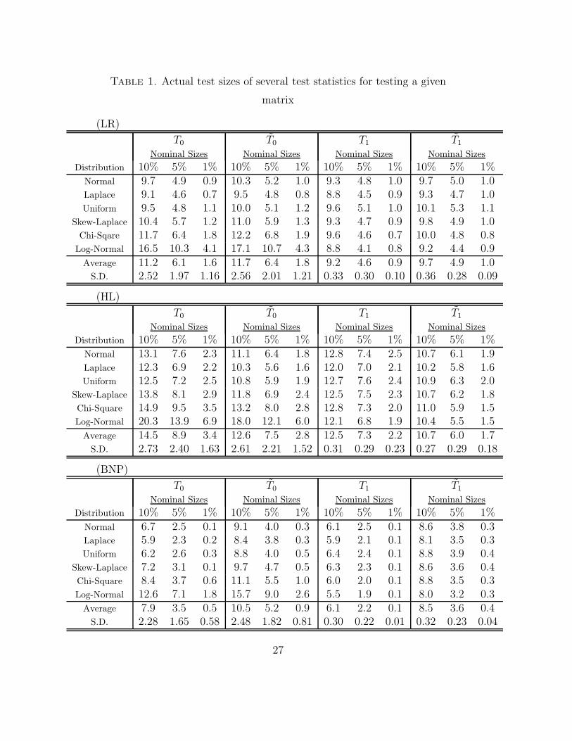
Table 1. Actual test sizes of several test statistics for testing a given
matrix
(LR)
T0 T0 T1 T1
Nominal Sizes Nominal Sizes Nominal Sizes Nominal SizesDistribution 10% 5% 1% 10% 5% 1% 10% 5% 1% 10% 5% 1%
Normal 9.7 4.9 0.9 10.3 5.2 1.0 9.3 4.8 1.0 9.7 5.0 1.0Laplace 9.1 4.6 0.7 9.5 4.8 0.8 8.8 4.5 0.9 9.3 4.7 1.0Uniform 9.5 4.8 1.1 10.0 5.1 1.2 9.6 5.1 1.0 10.1 5.3 1.1
Skew-Laplace 10.4 5.7 1.2 11.0 5.9 1.3 9.3 4.7 0.9 9.8 4.9 1.0Chi-Sqare 11.7 6.4 1.8 12.2 6.8 1.9 9.6 4.6 0.7 10.0 4.8 0.8
Log-Normal 16.5 10.3 4.1 17.1 10.7 4.3 8.8 4.1 0.8 9.2 4.4 0.9
Average 11.2 6.1 1.6 11.7 6.4 1.8 9.2 4.6 0.9 9.7 4.9 1.0S.D. 2.52 1.97 1.16 2.56 2.01 1.21 0.33 0.30 0.10 0.36 0.28 0.09
(HL)
T0 T0 T1 T1
Nominal Sizes Nominal Sizes Nominal Sizes Nominal SizesDistribution 10% 5% 1% 10% 5% 1% 10% 5% 1% 10% 5% 1%
Normal 13.1 7.6 2.3 11.1 6.4 1.8 12.8 7.4 2.5 10.7 6.1 1.9Laplace 12.3 6.9 2.2 10.3 5.6 1.6 12.0 7.0 2.1 10.2 5.8 1.6Uniform 12.5 7.2 2.5 10.8 5.9 1.9 12.7 7.6 2.4 10.9 6.3 2.0
Skew-Laplace 13.8 8.1 2.9 11.8 6.9 2.4 12.5 7.5 2.3 10.7 6.2 1.8Chi-Square 14.9 9.5 3.5 13.2 8.0 2.8 12.8 7.3 2.0 11.0 5.9 1.5Log-Normal 20.3 13.9 6.9 18.0 12.1 6.0 12.1 6.8 1.9 10.4 5.5 1.5
Average 14.5 8.9 3.4 12.6 7.5 2.8 12.5 7.3 2.2 10.7 6.0 1.7S.D. 2.73 2.40 1.63 2.61 2.21 1.52 0.31 0.29 0.23 0.27 0.29 0.18
(BNP)
T0 T0 T1 T1
Nominal Sizes Nominal Sizes Nominal Sizes Nominal SizesDistribution 10% 5% 1% 10% 5% 1% 10% 5% 1% 10% 5% 1%
Normal 6.7 2.5 0.1 9.1 4.0 0.3 6.1 2.5 0.1 8.6 3.8 0.3Laplace 5.9 2.3 0.2 8.4 3.8 0.3 5.9 2.1 0.1 8.1 3.5 0.3Uniform 6.2 2.6 0.3 8.8 4.0 0.5 6.4 2.4 0.1 8.8 3.9 0.4
Skew-Laplace 7.2 3.1 0.1 9.7 4.7 0.5 6.3 2.3 0.1 8.6 3.6 0.4Chi-Square 8.4 3.7 0.6 11.1 5.5 1.0 6.0 2.0 0.1 8.8 3.5 0.3Log-Normal 12.6 7.1 1.8 15.7 9.0 2.6 5.5 1.9 0.1 8.0 3.2 0.3
Average 7.9 3.5 0.5 10.5 5.2 0.9 6.1 2.2 0.1 8.5 3.6 0.4S.D. 2.28 1.65 0.58 2.48 1.82 0.81 0.30 0.22 0.01 0.32 0.23 0.04
27

Table 2. Robust design to nonnormality in testing the equality
(k = 4)
n1 : n2 : n3 : n41 : 1 : 2 : 4 1 : 2 : 2 : 5 1 : 2 : 4 : 41 : 3 : 4 : 4 2 : 5 : 5 : 10
(k = 5)
n1 : n2 : n3 : n4 : n5
1 : 1 : 1 : 3 : 3 1 : 1 : 3 : 3 : 31 : 3 : 3 : 3 : 5 3 : 5 : 5 : 7 : 153 : 5 : 8 : 12 : 12 3 : 7 : 7 : 10 : 15
(k = 6)
n1 : n2 : n3 : n4 : n5 : n6
2 : 3 : 4 : 5 : 8 : 8 2 : 3 : 5 : 5 : 5 : 103 : 3 : 3 : 4 : 5 : 12 3 : 4 : 4 : 4 : 9 : 123 : 4 : 6 : 6 : 6 : 15 3 : 6 : 6 : 8 : 10 : 153 : 9 : 9 : 9 : 12 : 14 4 : 5 : 5 : 5 : 12 : 154 : 5 : 12 : 12 : 12 : 15 4 : 8 : 10 : 15 : 16 : 164 : 10 : 10 : 10 : 15 : 20 5 : 8 : 12 : 15 : 20 : 20
28
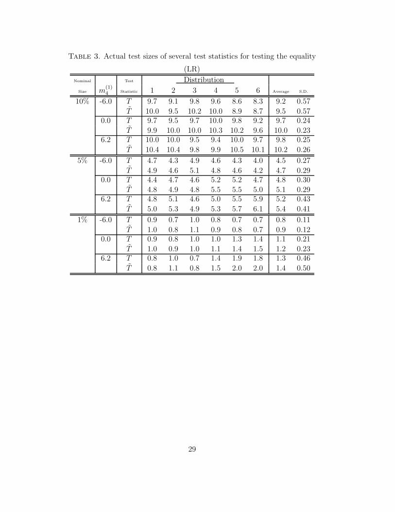
Table 3. Actual test sizes of several test statistics for testing the equality
(LR)
Nominal Test Distribution
Size m(1)4 Statistic 1 2 3 4 5 6 Average S.D.
10% -6.0 T 9.7 9.1 9.8 9.6 8.6 8.3 9.2 0.57
T 10.0 9.5 10.2 10.0 8.9 8.7 9.5 0.570.0 T 9.7 9.5 9.7 10.0 9.8 9.2 9.7 0.24
T 9.9 10.0 10.0 10.3 10.2 9.6 10.0 0.236.2 T 10.0 10.0 9.5 9.4 10.0 9.7 9.8 0.25
T 10.4 10.4 9.8 9.9 10.5 10.1 10.2 0.26
5% -6.0 T 4.7 4.3 4.9 4.6 4.3 4.0 4.5 0.27
T 4.9 4.6 5.1 4.8 4.6 4.2 4.7 0.290.0 T 4.4 4.7 4.6 5.2 5.2 4.7 4.8 0.30
T 4.8 4.9 4.8 5.5 5.5 5.0 5.1 0.296.2 T 4.8 5.1 4.6 5.0 5.5 5.9 5.2 0.43
T 5.0 5.3 4.9 5.3 5.7 6.1 5.4 0.41
1% -6.0 T 0.9 0.7 1.0 0.8 0.7 0.7 0.8 0.11
T 1.0 0.8 1.1 0.9 0.8 0.7 0.9 0.120.0 T 0.9 0.8 1.0 1.0 1.3 1.4 1.1 0.21
T 1.0 0.9 1.0 1.1 1.4 1.5 1.2 0.236.2 T 0.8 1.0 0.7 1.4 1.9 1.8 1.3 0.46
T 0.8 1.1 0.8 1.5 2.0 2.0 1.4 0.50
29
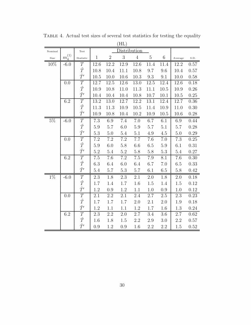
Table 4. Actual test sizes of several test statistics for testing the equality
(HL)
Nominal Test Distribution
Size m(1)4 Statistic 1 2 3 4 5 6 Average S.D.
10% -6.0 T 12.6 12.2 12.9 12.6 11.4 11.4 12.2 0.57
T 10.8 10.4 11.1 10.8 9.7 9.6 10.4 0.57
T ′ 10.5 10.0 10.6 10.3 9.3 9.1 10.0 0.580.0 T 12.7 12.5 12.6 13.0 12.5 12.4 12.6 0.18
T 10.9 10.8 11.0 11.3 11.1 10.5 10.9 0.26
T ′ 10.4 10.4 10.4 10.8 10.7 10.1 10.5 0.256.2 T 13.2 13.0 12.7 12.2 13.1 12.4 12.7 0.36
T 11.3 11.3 10.9 10.5 11.4 10.9 11.0 0.30
T ′ 10.9 10.8 10.4 10.2 10.9 10.5 10.6 0.28
5% -6.0 T 7.3 6.9 7.4 7.0 6.7 6.1 6.9 0.44
T 5.9 5.7 6.0 5.9 5.7 5.1 5.7 0.28
T ′ 5.3 5.0 5.4 5.1 4.9 4.5 5.0 0.290.0 T 7.2 7.2 7.2 7.7 7.6 7.0 7.3 0.25
T 5.9 6.0 5.8 6.6 6.5 5.9 6.1 0.31
T ′ 5.2 5.4 5.2 5.8 5.8 5.3 5.4 0.276.2 T 7.5 7.6 7.2 7.5 7.9 8.1 7.6 0.30
T 6.3 6.4 6.0 6.4 6.7 7.0 6.5 0.33
T ′ 5.4 5.7 5.3 5.7 6.1 6.5 5.8 0.42
1% -6.0 T 2.3 1.8 2.3 2.1 2.0 1.8 2.0 0.18
T 1.7 1.4 1.7 1.6 1.5 1.4 1.5 0.12
T ′ 1.2 0.9 1.2 1.1 1.0 0.9 1.0 0.120.0 T 2.1 2.2 2.1 2.4 2.7 2.5 2.3 0.23
T 1.7 1.7 1.7 2.0 2.1 2.0 1.9 0.18
T ′ 1.2 1.1 1.1 1.2 1.7 1.6 1.3 0.246.2 T 2.3 2.2 2.0 2.7 3.4 3.6 2.7 0.62
T 1.6 1.8 1.5 2.2 2.9 3.0 2.2 0.57
T ′ 0.9 1.2 0.9 1.6 2.2 2.2 1.5 0.52
30
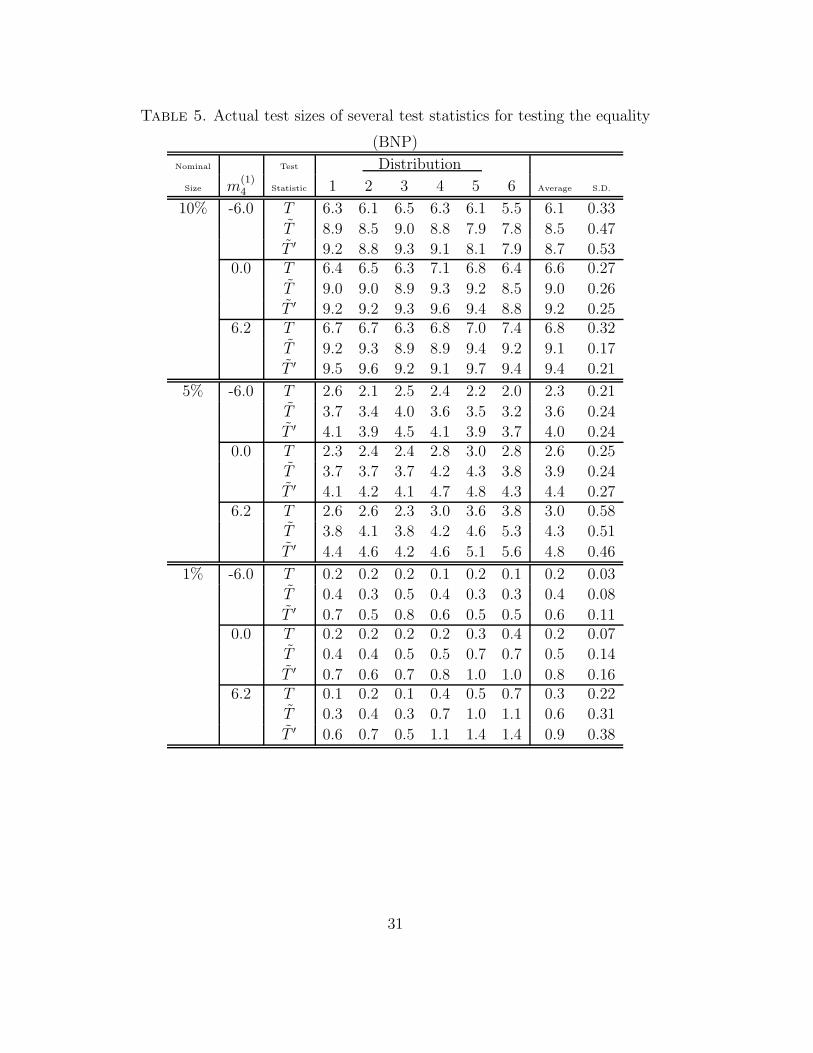
Table 5. Actual test sizes of several test statistics for testing the equality
(BNP)
Nominal Test Distribution
Size m(1)4 Statistic 1 2 3 4 5 6 Average S.D.
10% -6.0 T 6.3 6.1 6.5 6.3 6.1 5.5 6.1 0.33
T 8.9 8.5 9.0 8.8 7.9 7.8 8.5 0.47
T ′ 9.2 8.8 9.3 9.1 8.1 7.9 8.7 0.530.0 T 6.4 6.5 6.3 7.1 6.8 6.4 6.6 0.27
T 9.0 9.0 8.9 9.3 9.2 8.5 9.0 0.26
T ′ 9.2 9.2 9.3 9.6 9.4 8.8 9.2 0.256.2 T 6.7 6.7 6.3 6.8 7.0 7.4 6.8 0.32
T 9.2 9.3 8.9 8.9 9.4 9.2 9.1 0.17
T ′ 9.5 9.6 9.2 9.1 9.7 9.4 9.4 0.21
5% -6.0 T 2.6 2.1 2.5 2.4 2.2 2.0 2.3 0.21
T 3.7 3.4 4.0 3.6 3.5 3.2 3.6 0.24
T ′ 4.1 3.9 4.5 4.1 3.9 3.7 4.0 0.240.0 T 2.3 2.4 2.4 2.8 3.0 2.8 2.6 0.25
T 3.7 3.7 3.7 4.2 4.3 3.8 3.9 0.24
T ′ 4.1 4.2 4.1 4.7 4.8 4.3 4.4 0.276.2 T 2.6 2.6 2.3 3.0 3.6 3.8 3.0 0.58
T 3.8 4.1 3.8 4.2 4.6 5.3 4.3 0.51
T ′ 4.4 4.6 4.2 4.6 5.1 5.6 4.8 0.46
1% -6.0 T 0.2 0.2 0.2 0.1 0.2 0.1 0.2 0.03
T 0.4 0.3 0.5 0.4 0.3 0.3 0.4 0.08
T ′ 0.7 0.5 0.8 0.6 0.5 0.5 0.6 0.110.0 T 0.2 0.2 0.2 0.2 0.3 0.4 0.2 0.07
T 0.4 0.4 0.5 0.5 0.7 0.7 0.5 0.14
T ′ 0.7 0.6 0.7 0.8 1.0 1.0 0.8 0.166.2 T 0.1 0.2 0.1 0.4 0.5 0.7 0.3 0.22
T 0.3 0.4 0.3 0.7 1.0 1.1 0.6 0.31
T ′ 0.6 0.7 0.5 1.1 1.4 1.4 0.9 0.38
31
1 2 3 4 5 6
10
15
20
25Nominal 10% Test
Distributions
Act
ual S
ize
(%)
1 2 3 4 5 6
5
10
15
20Nominal 5% Test
Distributions
Act
ual S
ize
(%)
1 2 3 4 5 60
2
4
6
8
10
Nominal 1% Test
Distributions
Act
ual S
ize
(%)Nominal Size
One−Sample TestTwo−Sample Test
Distributions are:1. Normal 2. Laplace3. Uniform 4. Skew−Laplace5. Chi−Square 6. Log−Normal
Figure 1. Actual test sizes of Hotelling’s one- and two-sample tests
32