spectral decompositions and nonnormality of boundary ...people.bath.ac.uk/eas25/bephsp11.pdf ·...

IMA Journal of Numerical Analysis (2012) of 34doi:10.1093/imanum/drn000

Spectral decompositions and nonnormality of boundary integraloperators in acoustic scattering

T. BETCKE†, J. PHILLIPS‡, E. A. SPENCE§

[Received on 8 January 2012]

Understanding the spectral properties of boundary integral operators in acoustic scattering has importantpractical implications, such as for the analysis of the stability of boundary element discretisations or theconvergence of iterative solvers as the wavenumber k grows. Yet little is known about spectral decompo-sitions of the standard boundary integral operators in acoustic scattering. Theoretical results are mainlyavailable on the unit disk, where these operators diagonalise in a simple Fourier basis. In this paper weinvestigate spectral decompositions for more general smooth domains. Based on the decomposition ofthe acoustic Green’s function in elliptic coordinates we give spectral decompositions on ellipses. Forgeneral smooth domains we show that approximate spectral decompositions can be given in terms ofcircle Fourier modes transplanted onto the boundary of the domain. An important underlying question iswhether or not the operators are normal. Based on previous numerical investigations it appears that thestandard boundary integral operators are normal only when the domain is a ball and here we prove thatthis is indeed the case for the acoustic single layer potential. We show that the acoustic single, doubleand conjugate double layer potential are normal in a scaled inner product on the ellipse. On more generalsmooth domains the operators can be split into a normal component plus a smooth perturbation. Numeri-cal computations of pseudospectra are presented to demonstrate the nonnonnormal behaviour on generaldomains.

Keywords: acoustic scattering; boundary integral operators; spectra; pseudospectra

1. Introduction

The study of spectral properties of partial differential operators has seen tremendous advances in recentdecades. An important question is whether an operator is nonnormal and how this nonnormality influencesanalytical and numerical properties of the operator. The development of pseudospectra as a tool for under-standing nonnormality has given great insight into diverse areas, such as existence of solutions to linearPDE problems, the behaviour of numerical solvers, or transient behaviour in dynamical systems. For awonderful overview about this field we refer to the recent book by Trefethen & Embree (2005). How-ever, whilst nonnormality has been studied extensively for partial differential operators, little is known forboundary integral operators. The aim of this paper is to study nonnormality in the context of boundaryintegral operators in acoustic scattering.

Let Ω ⊂ R2 be a bounded domain and denote the boundary of Ω by Γ . For the majority of thispaper we assume that Γ is an analytic curve. Denote by Ω+ := R2\Ω the exterior of Ω . Furthermore,let g : R2×R2→ C be the acoustic Green’s function defined by g(x,y) = i

4 H(1)0 (k|x− y|), where k is the

wavenumber. We define the following operators, which are bounded operators on L2(Γ ) (for mappingproperties of these operators in Sobolev spaces see, for example, McLean (2000)).

• The acoustic single layer potential

[Sφ ](x) =∫

Γ

g(x,y)φ(y)ds(y), x ∈ Γ

†Department of Mathematics, University College London, UK. Corresponding author. Email: [email protected]. Timo Betcke issupported by Engineering and Physical Sciences Research Council (EPSRC) Grant EP/H004009/1.

‡Department of Mathematics, University College London, UK. Email: [email protected]. Joel Phillips is supported byEPSRC Grant EP/H004009/1.

§Department of Mathematics, University of Bath, UK. Email: [email protected]. Euan Spence is supported by EPSRC GrantEP/1025995/1.

c© The author 2012. Published by Oxford University Press on behalf of the Institute of Mathematics and its Applications. All rights reserved.

2 of 34 T. BETCKE, J. PHILLIPS, E. A. SPENCE

• The acoustic double layer potential

[Kφ ](x) =φ(x)

2+∫

Γ

∂

∂n(y)g(x,y)φ(y)ds(y), x ∈ Γ

• The acoustic conjugate double layer potential

[T φ ](x) =−φ(x)2

+∫

Γ

∂

∂n(x)g(x,y)φ(y)ds(y), x ∈ Γ

Here, n denotes the exterior normal to Ω . The double layer and conjugate double layer potentials usuallyappear without the factors of ±1/2. Our reason for defining them like this is that if we denote the exteriortrace operator by γ

+0 and the exterior normal derivative by γ

+1 , then the above boundary operators are

obtained from the single and double layer potentials,

[S φ ](x) =∫

Γ

g(x,y)φ(y)ds(y), [K φ ](x) =∫

Γ

∂

∂n(y)g(x,y)φ(y)ds(y), x ∈Ω

+

by S = γ+0 S , K = γ

+0 K , T = γ

+1 S . The fact that S,K, and T arise directly as the traces of S and K

makes the algebra of the spectral decompositions considered below more convenient. We will also beinterested in the combined potential operator

Aη := 2(I +T − iηS)

defined for η 6= 0. In Chandler-Wilde & Langdon (2007) it was shown that Aη is a bounded operator withbounded inverse for any k > 0, η 6= 0, mapping L2(Γ ) into L2(Γ ) for any Lipschitz boundary Γ .

The main motivation for studying the behaviour of these integral operators is that they can be usedto solve scattering problems modelled by the Helmholtz equation, with the combined potential operatorAη giving rise to a uniquely-solvable integral equation for the solution of the Helmholtz equation withDirichlet boundary conditions (see Section 6 for details). Another important boundary integral operatoris the hypersingular operator. This is γ

+1 K and arises when formulating boundary value problems for

the Helmholtz equation with Neumann boundary conditions. In this paper we are mainly focused on thebehaviour of the combined potential operator Aη and so we do not consider the hypersingular operator.

The spectral behaviour of the operators S, K, T and Aη is especially simple on the unit circle. We havethe following well known result (see e.g. Kress & Spassov (1983); Kress (1985); Domınguez et al. (2007)).

THEOREM 1.1 On the unit circle it holds that

Sun = λ(S)n un, Kun = λ

(K)n un, Tun = λ

(T )n un, Aη un = λ

(A)n un,

where in polar coordinates un(θ) = einθ and

λ(S)n =

πi2

H(1)n (k)Jn(k),

λ(K)n =

kπi4

H(1)n (k)(Jn−1(k)− Jn+1(k)) ,

λ(T )n =

kπi4

(H(1)

n−1(k)−H(1)n+1(k)

)Jn(k)

λ(A)n = 2(1+λ

(T )n − iηλ

(S)n ). (1.1)

Proof. The result is a consequence of the Graf addition formula (NIST Digital Library, eq. 10.23.7),stating that

H(1)0 (k|reiθ −ρeiφ |) =

∞

∑n=−∞

ein(θ−φ)H(1)n (kr>)Jn(kr<), (1.2)

where r> = max(r,ρ) and r< = min(r,ρ).

SPECTRAL DECOMPOSITIONS OF BOUNDARY INTEGRAL OPERATORS 3 of 34

(It is well known that on the unit circle K− 12 I = T + 1

2 I and this can be seen from the eigenvalues using

the facts that Jn−1(k)− Jn+1(k) = 2J′n(k), H(1)n−1(k)−H(1)

n+1(k) = 2H(1)′n (k), and W [Jn,H

(1)n ,k] = 2i/(πk),

where W denotes the Wronskian.)An important feature of the circle case is that the operators S, K, T and Aη are normal. since they

diagonalize in a unitary basis and therefore commute with their adjoints. Recall that a bounded operator Aacting on a Hilbert space H is normal if and only

AA∗ = A∗A,

where A∗ is the adjoint of A. Normal operators are simple in the sense that they can be shown to be unitarilyequivalent to multiplication operators (see for example (Conway, 1985, Theorem 4.6)). In particular, if Ais compact and normal then there exists an orthonormal system φ j, such that

A = ∑j

λ jφ j〈φ j, ·〉,

where the λ j are the eigenvalues of A and the φ j are the associated eigenfunctions. Hence, the behavior ofa normal operator can be completely determined by spectral information.

For more general domains than the circle, little is known about spectral decompositions, however un-derstanding the spectral properties and normality of these boundary integral operators has both theoreticaland practical implications. On the theoretical side, in Ramm (1973, 1980) Ramm asked when the eigen-system of the single layer potential operator in 3-d forms a complete basis in L2(Γ ) and gave normality asa sufficient condition. On the practical side, whether an operator is normal or not affects the convergenceof iterative solvers such as GMRES.

An important question, therefore, is whether the operators S, K, T and Aη are normal on any domainsother than the circle (in 2-d, or sphere in 3-d). Numerical experiments in Betcke & Spence (2011) demon-strate that the combined potential operator Aη appears to be nonnormal on a wide range of 2-d domains,which leads to the question of whether the circle is the only 2-d domain on which these operators are nor-mal. In this paper we prove for the single layer potential operator S that, amongst all sufficiently smooth 2-dand 3-d domains, balls are the only domains for which the operator is normal in the standard L2(Γ ) innerproduct (see Theorem 3.1 below). The rest of this paper is, in some sense, an investigation into whetherthe desirable property of normality can be recovered, either in special cases or approximately.

If the Helmholtz equation is separable in a particular orthogonal coordinate system, then the Green’sfunction can be expanded in terms of special functions ((1.2) is this expansion for polar coordinates), andthis allows the derivation of eigenvalue decompositions of the operators S,K, and T for certain domains.We show that these decompositions lead to the operators being normal in a modified L2 inner product, anddemonstrate this in the case on an ellipse.

The explicit eigenvalue decompositions above are only possible for a very restrictive class of domains.Nevertheless, for arbitrary smooth domains we derive an approximate eigenvalue decomposition that relateseigenvalues on smooth domains to eigenvalues on the unit circle. In particular, it allows us to separatethe spectrum into O(k) eigenvalues that are not well approximated by circle eigenvalues, and a tail ofeigenvalues that are well-approximated by circle eigenvalues with associated approximate eigenfunctionsthat are orthogonal in a modified L2 inner product. This result shows that nonnormality appears mainly toaffect a finite number of O(k) eigenvalues.

The paper is organized as follows. In Section 2 we briefly introduce two related tools for the studyof nonnormality, namely pseudospectra and numerical ranges. We then demonstrate the effect of nonnor-mality on norm bounds and on coercivity constants for boundary integral operators in acoustic scattering.In Section 3 we present a proof that, amongst all sufficiently smooth domains, circles (respectively ballsin 3-d) are the only ones for which the acoustic single layer potential is normal. The proof is based ontransforming the question of normality into a uniqueness problem of equilibrium potentials, which hasbeen solved by Reichel (1997). In Section 4 we use the decomposition of the acoustic Green’s function inelliptic coordinates to derive an eigenvalue decomposition of the operators S, K and T on the boundary ofan ellipse. This allows one to prove that these operators are normal in a scaled L2 inner product. In Section5 approximate eigendecompositions are derived for general analytic domains. Applications of the resultsto the combined potential operator Aη are treated in Section 6. Numerical examples will be given for twodomains. The paper finishes with conclusions in Section 7.


Notation in this paper is mostly standard. Unless otherwise stated we use ‖ · ‖ for the norm induced bythe standard complex L2(Γ ) inner product

(u,v) :=∫

Γ

u(s)v(s)ds,

where Γ is the boundary of a given domain. For disambiguation we will also use from time to time thesymbols ‖ · ‖L2(Γ ) and (·, ·)L2(Γ ) to emphasise the standard L2(Γ ) norm and inner product. Frequently wewill make use of a scaled L2 inner product defined by

(u,v)L2(F−1,Γ ) :=∫

Γ

(F−1u)(y)v(y)ds(y)

and the induced norm

‖v‖L2(F−1,Γ ) :=(∫

Γ

(F−1v)(y)v(y)ds(y))1/2

,

where F is a given multiplication operator.

2. Nonnormality and its consequences for the solution of boundary integral equations

In this section we first give a brief introduction to two widely used tools for the analysis of nonnormality,namely pseudospectra and numerical ranges. Then by looking at norms and coercivity constants we giveexamples of how nonnormality influences the behavior of boundary integral operators.

2.1 Pseudospectra and numerical ranges of operators

A widely used tool for investigating nonnormality is via the pseudospectrum of an operator. It can becharacterised by the following three equivalent definitions (Trefethen & Embree, 2005).

DEFINITION 2.1 (Pseudospectrum of a bounded operator) Let A be a bounded operator on a Hilbert spaceH and ε > 0 be arbitrary: The ε-pseudospectrum σε(A) of A is the set of z ∈ C defined equivalently byany of the conditions

1. ‖(z−A)−1‖> ε−1.

2. z ∈ σ(A+E) for some bounded operator E with ‖E‖< ε .

3. z ∈ σ(A) or ‖(z−A)u‖< ε for some u ∈H with ‖u‖= 1.

If ‖(z−A)u‖< ε with ‖u‖= 1 then z is an ε-pseudoeigenvalue of A and u is a corresponding ε-pseudoeigenvector(or pseudoeigenfunction or pseudomode).

The definition in (Trefethen & Embree, 2005, Chapter 4) is stated in terms of closed operators actingon Banach spaces. However, in this paper we are only interested in bounded Hilbert space operators. Fornormal matrices the ε-pseudospectrum is just the union of open disks of radius ε around the spectral values.In general, if A is nonnormal the form of the pseudospectra can be very different.

A rougher but also very useful tool to investigate nonnormality is the numerical range of a boundedlinear operator A acting on a Hilbert space H . It is defined as

W (A) := 〈Au,u〉, u ∈H , ‖u‖= 1.

The numerical range is always a convex set such that the spectrum σ(A)⊂W (A). Furthermore, the closureof the numerical range of a normal operator is the convex hull of its eigenvalues. There exists a simplerelationship between the numerical range and the ε-pseudospectrum, namely

σε(A)⊂W (A)+∆ε ,


−1.5 −1 −0.5 0 0.5 1 1.5

−1

−0.5

0

0.5

1

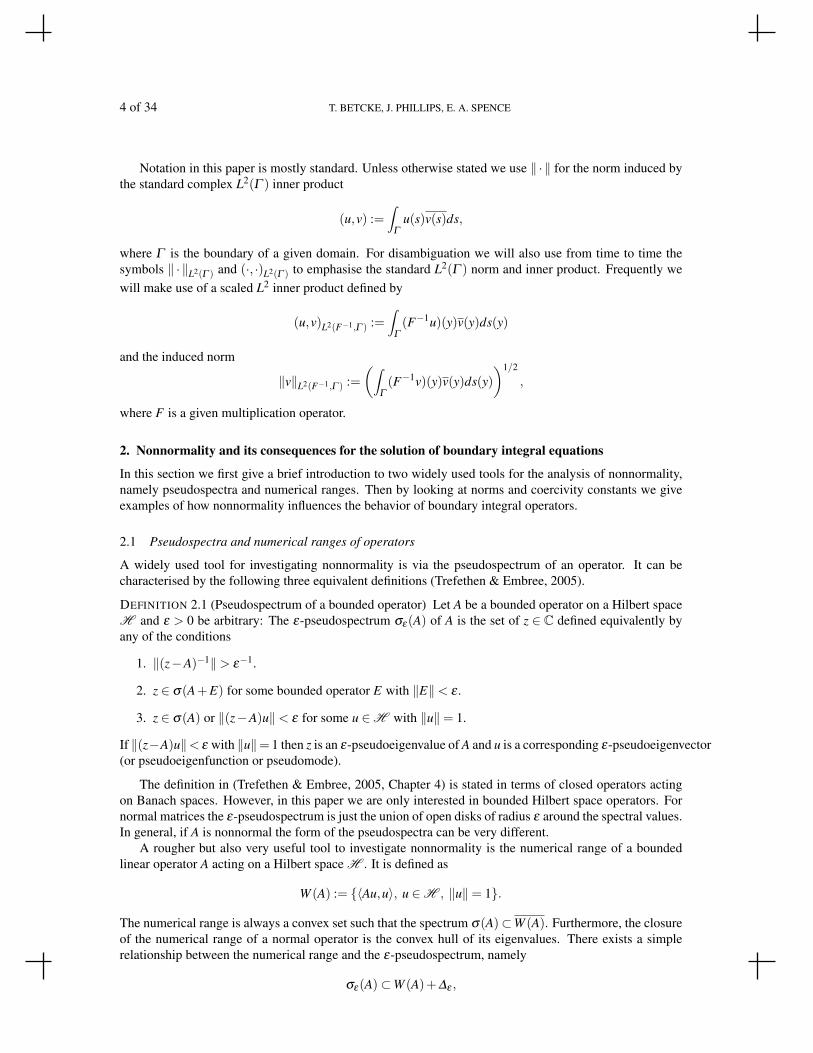
FIG. 1: A crescent domain parameterised by z(t) = eit − 0.1eit+0.9 , t ∈ [0,2π].

−0.5 0 0.5 1 1.5 2 2.5 3 3.5 4 4.5 5

−3

−2.5

−2

−1.5

−1

−0.5

0

0.5

1

1.5

2

−2.5

−2.25

−2

−1.75

−1.5

−1.25

−1

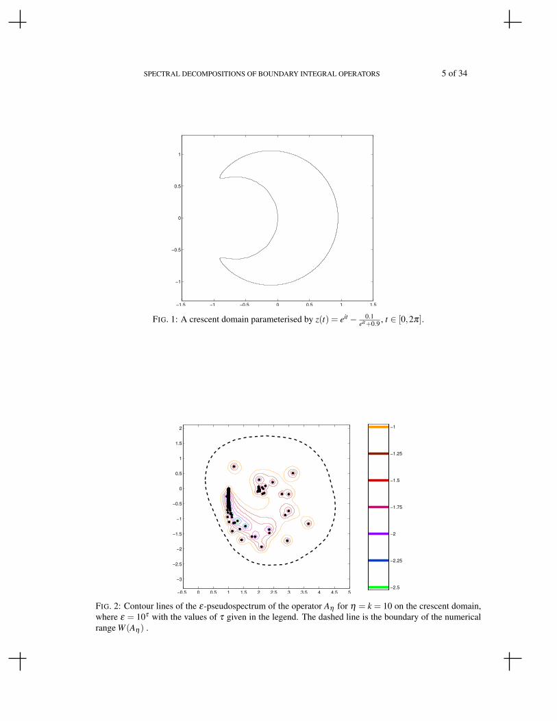
FIG. 2: Contour lines of the ε-pseudospectrum of the operator Aη for η = k = 10 on the crescent domain,where ε = 10τ with the values of τ given in the legend. The dashed line is the boundary of the numericalrange W (Aη) .


10−1

100

101

102

10−2

10−1

100

101

k

||S||

||K||

||T||

FIG. 3: The norm of the operators ‖S‖, ‖K‖ and ‖T‖ on the unit circle.

where ∆ε is the open disk around the origin of radius ε (Trefethen & Embree, 2005, Chapter 17). In Figure2 we plot the ε-pseudospectrum and the numerical range for the combined potential operator Aη in L2(Γ )with η = k = 10 for the crescent domain shown in Figure 1 (see Section 6 for more examples and details ofthe computation). The differently coloured contour lines are the boundaries of the ε-pseudospectrum forε = 10τ , where τ are the values given in the legend. The dashed line is the boundary of the numerical rangeand the dots are the eigenvalues. It is clear from this plot that the operator is not normal. The numericalrange is much larger than the convex hull of the eigenvalues. The ε-pseudospectrum was computed usingEigTool, a Matlab software package developed by Wright (2002).

2.2 Norm estimates

If the compact operator A is normal then by diagonalisation in its eigenbasis it follows that

‖A‖= supn|λn(A)|.

This was used in Domınguez et al. (2007) to give estimates for the k-dependence of the norm of combinedboundary integral operators on the circle in 2-d and the sphere in 3-d (following similar investigations byKress & Spassov (1983), Kress (1985)). From the analysis in (Domınguez et al., 2007, Section 4) it followsthat

‖S‖6Ck−2/3, ‖K‖6Ck1/3

for the circle. Numerical experiments in Betcke et al. (2011) indicated that a sharper bound on ‖K‖ is

‖K‖6C.

Indeed, this bound was proved for the unit sphere in 3-d in Banjai & Sauter (2007), and since the eigen-values for the unit sphere are very similar to the eigenvalues for the unit circle this bound also holds forthe unit circle. In Figure 3 we show the k-dependence of the norm of the operators S, K and T on the unitcircle. For the BEM discretisation we used roughly 30 elements per wavelength and quadratic polynomialsas basis functions on each element. The results were computed by taking the maximum over the absolutevalues of the first 100 eigenvalues computed from the formulas in Theorem 1.1. These computation con-


100

101

102

10−2

10−1

100

101

k

|λ

max|

\|S\|

FIG. 4: Absolute value of the largest eigenvalue λmax(S) and ‖S‖L2(Γ ) of the single layer potential S on theboundary of the crescent domain from Figure 1 for growing values k.

firm both the O(k−2/3) decay for the single layer potential and the fact that the norms of K and T behavelike O(1) independently of k.

If A is nonnormal we cannot use eigenvalues to bound the norm since in general we only have

supn|λn(A)|6 ‖A‖.

In Figure 4 we demonstrate the difference of |λmax| := supn |λn| and ‖S‖L2(Γ ) for the single layer potentialon the boundary Γ for the crescent domain from Figure 1. Numerically, for the eigenvalues we obtain adecay of approximately O(k−0.77), while the norm decays much slower with a rate of about O(k−1/2). Thiseffect is a consequence of nonnormality. In Betcke et al. (2011) various norm estimates are summarised;for general Lipschitz domains the estimate ‖S‖L2(Γ ) = O(k−1/2) holds.

There is an interesting relationship between the norm of an operator and its numerical range. Letr(A) := sup|z| : z∈W (A) be the numerical radius of A. Then it holds that r(A)6 ‖A‖6 2r(A) (Gustafson& Rao, 1997). Hence, k-dependent norm bounds immediately are also bounds for the extent of the numer-ical range of the operators S, K and T .

2.3 Coercivity Constants

An operator A acting on a Hilbert space H is coercive if there exists γ > 0, such that

γ‖u‖2 6 |〈Au,u〉|

for all u ∈H . Consider the abstract variational problem

Find u ∈H , such that 〈Au,v〉= f (v), ∀v ∈H , (2.1)

where f ∈H ′. Let V (h) be a finite dimensional subspace of H and dente by u(h) the solution of thevariational problem (2.1) restricted to V (h). Then if A is coercive, by Cea’s Lemma, (Cea, 1964), we have

‖u−u(h)‖6C minv∈V (h)

‖u(h)− v‖, (2.2)


where C = ‖A‖/γ .The analysis of coercivity constants for the combined potential operator Aη is the subject of current re-

search (see Spence et al. (2011)), and the main motivation for this is the following. Recall that establishingcoercivity means that the quasi-optimality estimate (2.2) holds for any finite dimensional subspace V (h).Recently much research effort has gone into designing k-dependent subspaces that accurately approximatethe solution to scattering problems where k is large, even for relatively small subspace dimension. (Recallthat the standard piecewise polynomial subspaces require their dimension to grow like kd−1 to maintainaccuracy as k increases.) An overview of these “hybrid numerical-asymptotic” methods can be found inthe review by Chandler-Wilde & Graham (2009). Since these subspaces depend on k in a complicated way,the only known way of proving convergence of Galerkin methods using these subspaces is via coercivity.

A first coercivity proof for Ak in L2(Γ ) was given in Domınguez et al. (2007) for the case that Γ isthe unit circle or the unit sphere. By a careful analysis of the eigenvalues of Ak it was shown that γ > 1for sufficiently large k. For general domains an eigenvalue analysis is not sufficient any more. This canbe seen as follows. From the definition of the numerical range it follows that Aη is coercive if and onlyif 0 6∈W (Aη). Furthermore, if Ak is coercive then γ is just the distance of 0 to W (Ak). In the case ofthe circle the combined potential operator is normal and the numerical range is just the convex hull of theeigenvalues. But this need not be the case for more general domains. However, we can still numericallystudy the distance of the origin to the boundary of the numerical range in order to estimate coercivityconstants. This was recently done in Betcke & Spence (2011). As an example consider the numericalrange plot in Figure 2 for Ak defined on the boundary of the crescent domain. From the plot it follows thatAk is coercive with a coercivity constant smaller than 0.5. It is instructive to compare the boundary of thenumerical range with the eigenvalues. The boundary of W (Ak) is much closer to 0 than the eigenvalues, aneffect due to the nonnormaliity of the operator.

3. A nonnormality proof for the single layer potential operator

It was observed in (Betcke & Spence, 2011, Lemma 3.5) that Aη is normal in L2(Γ ) if Γ is the boundaryof a circle in 2-d or a sphere in 3-d. Using the same argument S, K and T are also normal on the circleand sphere. In this section we provide a partial answer to the question of whether there are any domains,other than the circle and sphere, for which the operators S, K, T and Aη are normal in the standard L2(Γ )inner product. By reformulating the problem of normality into one of equilibrium potentials we prove thatamong all bounded C2,α domains balls are the only ones for which the operator S is normal. The mainresult is the following theorem.

THEOREM 3.1 Let Ω ⊂ Rd , d = 2,3 be a bounded C2,α domain with boundary Γ . Then the single layerpotential S is normal if and only if Ω is a ball.

The proof that S is normal on a ball follows by diagonalisation in the Fourier-basis (2-d) and by diago-nalisation in spherical harmonics (3-d), see (Betcke & Spence, 2011, Lemma 3.5) for details. To prove theconverse we first show that S normal implies that the logarithmic single layer potential operator defined by

[S0φ ](x) :=

− 1

2π

∫Γ

log |x− y|φ(y)ds(y), 2-d1

4π

∫Γ

1|x−y|φ(y)ds(y), 3-d

applied to the constant function 1 is constant inside Ω . We can then use the following result to show thatΩ must be a ball.

THEOREM 3.2 (Theorem 2 and §3 of Reichel (1997)) If Ω is a C2,α domain and S01 is constant in Ω thenΩ is a ball.

This problem can be understood in terms of equilibrium potentials (see, e.g., (Ransford, 1995, §3.3)).Given a domain, the nontrivial measure that gives rise to a constant potential throughout the domain iscalled the equilibrium measure. The corresponding potential is the equilibrium potential. Theorem 3.2states that the potential S01 is the equilibrium potential only for the case when Ω is a ball. The proof inReichel (1997) considers the equivalent problem of showing that the following overdetermined boundary


value problem has a solution if and only if Ω is a ball:

∆w = 0 in Ω , γ+1 w =−1, γ

+0 w = a,

where a is a constant and an appropriate condition at infinity is prescribed. This condition at infinity isu→ 0 for d > 3, and one involving layer potentials for d = 2 (since the single layer potential does notdecay at infinity in this case).

These overdetermined problems in potential theory have a long history, beginning with the celebratedwork of Serrin (1971), and are motivated by physical questions including stress in hydrodynamics.

A natural question is where the restriction that C2,α comes from. In order to apply the appropriatetheorem on the overdetermined problem, (Reichel, 1997, Theorem 1), Reichel requires that S01 be inC2(Ω+). Reichel uses a special case of a general regularity theorem (Gilbarg & Trudinger, 1998, Theorem6.14) to show that if D is a C2,α domain, ∆u = 0 in D, and the boundary data is C2,α , then u ∈C2,α(D).

In order to proof Theorem 3.1 from Theorem 3.2 we need to show that if the acoustic single layerpotential S is normal then S01 is constant in Ω . The next lemma is technical and gives a reformulation ofthe condition that S is normal.

LEMMA 3.1 Let the acoustic Green’s function g(x,y) = u(|x− y|)+ iv(|x− y|) where u and v are real. S isnormal if and only if

C(x,z) :=∫

Γ

u(|z− y|)v(|x− y|)−u(|x− y|)v(|z− y|)ds(y) = 0 (3.1)

for all x,z ∈ Γ .

Proof. Given f ∈ L2(Γ )

[(SS∗−S∗S) f ](x) =∫

Γ

∫Γ

(g(x,y)g(z,y)−g(y,x)g(y,z)) f (z)ds(z)ds(y)

=∫

Γ

∫Γ

2i(u(|z− y|)v(|x− y|)−u(|x− y|)v(|z− y|)) f (z)ds(z)ds(y)

= 2i∫

Γ

f (z)C(x,z)ds(z) (3.2)

where x,z ∈ Γ . Interchanging the order of integration is justified by Fubini’s theorem since g is weaklysingular.

Assume that S is normal, that is SS∗−S∗S = 0. Given any arbitrary z′ ∈ Γ , the right hand side of (3.2)can be made arbitrarily close to 2iC(x,z′) by choosing an appropriate f (z) with support in a neighbourhoodof z′. Thus if (SS∗−S∗S)( f )(x) is equal to zero for all x ∈ Γ and for all f then C(x,z′) = 0 for all x,z′ ∈ Γ .The converse is immediate.

We know that S is normal for Γ the circle or sphere, and we can check that C(x,z) = 0 in this case.Indeed, the change of variables y = (x+z)−y′ transforms the unit circle/sphere centered at 0 to one centredat x+ z, and ds(y) = ds(y′). Making this change of variables in the second term in (3.1) we see that, since|z− y|= |x− y′| and |x− y|= |z− y′|, the second term cancels with the first and thus C(x,z) = 0.

For the next lemma we note that for d = 2, u(r) =− 14Y0(kr) and v(r) = 1

4 J0(kr), where Jν and Yν areBessel functions of the first and second kind respectively. For d = 3, g(x,y) = eik|x−y|/(4π|x−y|) and thusu(r) = (coskr)/(4πr) and v(r) = (sinkr)/(4πr).

We can now prove the following.

LEMMA 3.2 If C(x,z) = 0 for all x,z ∈ Γ then S01 is constant in Ω .

Proof. Since C(x,z) = 0 for all x,z ∈ Γ , then of course for every fixed z C(x,z) = 0 for all x ∈ Γ . Thus,∇Γ ,xC(x,z) = 0 for all x ∈ Γ , where ∇Γ ,x is the surface gradient. An explicit expression for this in termsof a parametrisation of the boundary can be found in (Monk, 2003, §3.4) (Colton & Kress, 1983, §2.1) forsmooth domains. Furthermore, if w is C1 in a neighbourhood of Γ then

∇Γ ,xw(x) = ∇w(x)−n(x)∂w∂n

(x), x ∈ Γ . (3.3)


Ideally we would like to take ∇Γ ,x under the integral sign in the definition of C(x,z) (3.1) and obtain

∇Γ ,xC(x,z) = P.V.∫

Γ

(x− y|x− y|

− (x− y) ·n(x)|x− y|

n(x))(

u(|z− y|)v′(|x− y|)−u′(|x− y|)v(|z− y|))

ds(y)

(3.4)

where we are using (3.3) to find the surface gradient of |x− y| under the integral sign. However, since theintegrand is weakly singular, this interchange of integration and differentiation requires some justification.

The key result is that, for φ ∈ L2(Γ ) and k > 0,

∇Γ ,x[Sφ ](x) = [∇Γ Sφ ](x) (3.5)

where the right hand side is the integral operator defined by

[∇Γ Sφ ](x) = P.V.∫

Γ

∇Γ ,xg(x,y)φ(y)ds(y), (3.6)

= P.V.∫

Γ

(x− y|x− y|

− (x− y) ·n(x)|x− y|

n(x))(u′(|x− y|)+ iv′(|x− y|))φ(y)ds(y). (3.7)

On C2 domains this follows from the results for Holder continuous φ in (Colton & Kress, 1983, Theorem2.17) (using the density of Holder continuous functions in L2(Γ ) when Γ is C2), and this result is true evenon Lipschitz domains by the harmonic analysis results surveyed in (Meyer & Coifman, 2000, Chapter 15).

The result (3.5) justifies (3.4) as follows. C, defined by (3.1), consists of two terms: the first, viewedas a function of x, is the imaginary part of the single layer potential with density u(|z− y|), the second,again viewed as a function of x, is the real part of the single layer potential with density v(|z− y|). Bothu(|z− y|) and v(|z− y|) are in L2(Γ ) and thus interchanging the differentiation and integration is justifiedby the imaginary and real parts respectively of (3.5).

Since ∇Γ ,xC(x,z) = 0 for all x ∈ Γ in particular this holds for x = z. Let χ(z) := ∇Γ ,xC(x,z)|(x=z).Then, for d = 2 the Wronskian u(r)v′(r)−u′(r)v(r) =−1/(2πkr) and

χ(z) = P.V.∫

Γ

(z− y|z− y|

− (z− y) ·n(z)|z− y|

n(z))

−12πk |z− y|

ds(y) =− 12πk

∇Γ ,z

∫Γ

log(|z− y|)ds(y), d = 2,

(where taking the surface gradient out from under the integral sign is justified by (3.5) above with k = 0).For d = 3, the Wronskian u(r)v′(r)−u′(r)v(r) = k/(4πr2) and

χ(z) = P.V.∫

Γ

(z− y|z− y|

− (z− y) ·n(z)|z− y|

n(z))

k4π|z− y|2

ds(y) =k

4π∇Γ ,z

∫Γ

1|z− y|

ds(y), d = 3.

Thus C(x,z) = 0 for all x,z ∈ Γ implies that χ(z) = 0 for all z ∈ Γ and thus [S01](z) is constant for allz ∈ Γ . Since S01 is harmonic, by the maximum principle it is constant in Ω .

By combining Lemma 3.1 and Lemma 3.2 we can apply Theorem 3.2 to show that if S is normal thenΩ must be a ball. This concludes the missing direction of the proof of Theorem 3.1.

4. The spectrum on the boundary of an ellipse

4.1 Eigendecomposition in elliptic coordinates

The main ingredient for computing an eigenvalue expansion on the disk is the Graf addition formula thatgives an expansion of the acoustic Green’s function in a polar coordinate system. In this section we gen-eralise these results to an ellipse by using an elliptic coordinate system and an expansion of the acousticGreen’s function in elliptic coordinates. A significant difference to the disk case is that the natural param-eterisation of the boundary of an ellipse in elliptic coordinates has a non-constant Jacobian. The effect isthat instead of a simple eigenvalue expansion for the single layer potential S we will arrive at a generalisedeigenvalue expansion of the form SF−1un = λnun, where F is a simple scaling operator. For the case ofboundary integral operators in harmonic potential theory eigenvalue expansions on the ellipse were derived


by Rodin & Steinbach (2003). For the Helmholtz case we need Mathieu functions, which we will brieflyintroduce here.

Let Ω be an ellipse with boundary Γ parameterised by γ(ν) :=[

acosh µ cosν

asinh µ sinν

]. Define q = 1

4 (ka)2.

Separation of variables of the Helmholtz equation in elliptic variables leads to the standard Mathieu equa-tion

N′′(ν)+(λ −2qcos2ν)N(ν) = 0 (4.1)

and the modified Mathieu equation

M′′(µ)− (λ −2qcosh2µ)M(µ) = 0, (4.2)

where λ is a separation constant. Together with suitable boundary conditions (4.1) is a Sturm-Liouvilleproblem, where λ = λ (q) is the eigenvalue parameter. Depending on the boundary conditions two sets ofeigenvalues an(q) and bn(q) are defined (NIST Digital Library, §28.2(v)). By cen(ν ,q) we denote the eveneigenfunctions associated with the eigenvalues an(q) and by sen(ν ,q) the odd eigenfunctions associatedwith bn(q). (NIST Digital Library, §28.2(vi)). These form an orthogonal basis of L2[0,2π]. For thenormalisation of the functions we use the standard choice∫ 2π

0ce2

n(ν ,q)dν =∫ 2π

0se2

n(ν ,q)dν = π.

For the modified Mathieu equation (4.2) we introduce the two sets of solutions Mc(1)n (µ,q) and Mc(2)n (µ,q)associated with the eigenvalues an(q). From these the modified Mathieu functions Mc(3/4)

n are defined by

Mc(3/4)n (µ,q) = Mc(1)n (µ,q)± iMc(2)n (µ,q).

Mc(1)n is the elliptic analogue of the Bessel function Jn and Mc(2)n is the elliptic analogue of the Besselfunction of the second kind Yn. Indeed, it holds that (NIST Digital Library, eq. 28.20.10,28.20.15-16)

Mc(3/4)n (µ,q)∼ H(1/2)

n (2q1/2 cosh µ) as µ → ∞. (4.3)

One defines the functions Ms(1/2)n and Ms(3/4)

n associated with the eigenvalues bn(q) similarly.Similar to the circle case, there exists an expansion of the acoustic Green’s function in elliptic coordi-

nates.

THEOREM 4.1 (Expansion of fundamental solution in Mathieu functions)

i4

H(1)0 (k|x− y|) = i

2

(∞

∑m=0

cem(ν ,q)cem(ν′,q)Mc(1)m (µ<,q)Mc(3)m (µ>,q)

+∞

∑m=1

sem(ν ,q)sem(ν′,q)Ms(1)m (µ<,q)Ms(3)m (µ>,q)

)(4.4)

where x = (acosh µ cosν ,asinh µ sinν), y = (acosh µ ′ cosν ′,asinh µ ′ sinν ′) and µ> = max(µ,µ ′), µ< =min(µ,µ ′)

Proof. This formula can be found in (Morse & Feshbach, 1953a, §11.2). However, it is not deriveddirectly, but is quoted as a special case of a general technique described in (Morse & Feshbach, 1953b,§7.2). Furthermore, the notation for Mathieu functions used in these references is not the (now fairlystandard) notation used in the Digital Library of Mathematical Functions that we use here. Because ofthese complications we give a full derivation of this expansion in Appendix B.

We cannot quite proceed as in the case of the unit circle. On the ellipse the boundary measure ds isnot identical to the angular measure dν since |γ ′(ν)| 6= const. We have to introduce an additional scalingoperator F to take this into account.

THEOREM 4.2 Let Γ be the boundary of an ellipse and x = γ(s) be its parameterisation in elliptic coordi-nates as defined above. Denote by µ the radius of the ellipse in elliptic coordinates associated with the pa-rameter q = 1

4 (ka)2. Define the multiplication operator F : L2(Γ )→ L2(Γ ) by [Fφ ](x) = |γ ′(γ−1(x))|φ(x).The following eigenvalue decompositions hold.


• For the single layer potential S:

SF−1φ(c)j = λ

(S,c)j φ

(c)j

SF−1φ(s)j = λ

(S,s)j φ

(s)j ,

whereλ(S,c)j =

iπ2

Mc(1)j (µ,q)Mc(3)j (µ,q), λ(S,s)j =

iπ2

Ms(1)j (µ,q)Ms(3)j (µ,q)

• For the double layer potential K:

Kφ(c)j = λ

(K,c)j φ

(c)j

Kφ(s)j = λ

(K,s)j φ

(s)j ,

where

λ(K,c)j =

iπ2

[∂

∂ µMc(1)j (µ,q)

]Mc(3)j (µ,q), λ

(K,s)j =

iπ2

[∂

∂ µMs(1)j (µ,q)

]Ms(3)j (µ,q).

• For the conjugate double layer potential T:

FT F−1φ(c)j = λ

(T,c)j φ

(c)j

FT F−1φ(s)j = λ

(T,s)j φ

(s)j ,

where

λ(T,c)j =

iπ2

Mc(1)j (µ,q)[

∂

∂ µMc(3)j (µ,q)

], λ

(T,s)j =

iπ2

Ms(1)j (µ,q)[

∂

∂ µMs(3)j (µ,q)

].

In all three cases the eigenfunctions φ(c)j and φ

(s)j are defined as

φ(c)j (x) = ce j(γ

−1(x),q), φ(s)j (x) = se j(γ

−1(x),q).

Proof. From the decomposition of the acoustic Green’s function in Theorem 4.1 and the orthogonality ofMathieu functions with respect to the inner product (·, ·)L2([0,2π]) it follows for x=(acosh µ cosν ,asinh µ sinν)that

[SF−1φ(c)j ](x) =

∫Γ

i4

H(1)0 (k|x− y|)

φ(c)j (y)

|γ ′(γ−1(y))|ds(y)

=∫ 2π

0|γ ′(t)| i

4H(1)

0 (k|x− γ(t)|)ce j(t,q)|γ ′(t)|

dt

=iπ2

Mc(1)j (µ,q)Mc(3)j (µ,q)ce j(ν ,q)

= λ(S,c)j φ

(c)j (x).

For the double layer and conjugate double layer potential we first note that ∂

∂n(x) =1

|γ ′(γ−1(x))|∂

∂ µfor

x ∈ Γ since elliptic coordinates are an orthogonal coordinate system. Let x ∈ Ω+ have the representation(µ,ν) in elliptic coordinates. It follows that

[K φ(c)j ](x) =

∫Γ

∂

∂n(y)i4

H(1)0 (k|x− y|)ce j(γ

−1(y),q)ds(y)

=iπ2

[∂

∂ µMc(1)j (µ,q)

]Mc(3)j (µ,q)ce j(ν ,q). (4.5)


Since Ku = γ+0 K for u ∈ L2(Γ ) the result follows for µ → µ . For the conjugate double layer potential we

note that[S F−1

φ(c)j ](x) =

iπ2

Mc(1)j (µ,q)Mc(3)j (µ,q)ce j(ν ,q),

giving

[FT F−1φ(c)j ](x) = [Fγ

+1 S F−1

φ(c)j ](x) =

iπ2

Mc(1)j (µ,q)[

∂

∂ µMc(3)j (µ,q)

]ce j(ν ,q)

for x ∈ Γ . The calculations for φ(s)j are similar.

The operator F is positive definite with bounded inverse on L2(Γ ). We can therefore define the innerproduct

(u,v)L2(F−1,Γ ) :=∫

Γ

(F−1u)(y)v(y)ds(y)

and associated norm

‖v‖L2(F−1,Γ ) :=(∫

Γ

(F−1v)(y)v(y)ds(y))1/2

for all v in L2(Γ ). Since asinh µ 6 |γ ′(t)|6 acosh µ for all t ∈ R it follows that

1√acosh µ

‖ · ‖L2(Γ ) 6 ‖ · ‖L2(F−1,Γ ) 61√

asinh µ‖ · ‖L2(Γ ).

We can now proof a simple normality result with respect to this scaled inner product.

THEOREM 4.3 The operators SF−1, K and FT F−1 are normal with respect to the inner product (u,v)L2(F−1,Γ ).

Proof. For any two functions u,v ∈ L2(Γ ) we have

(u,v)L2(F−1,Γ ) =∫

Γ

(F−1u)vds =∫ 2π

0u(γ(t))v(γ(t))dt.

Hence, from the orthogonality of the Mathieu functions ce j and se j with respect to the standard L2([0,2π])

inner product it follows that the functions φ(c)j and φ

(s)j are orthogonal with respect to the inner product

(·, ·)L2(F−1,Γ ). Together with Theorem 4.2 it therefore follows that the operators SF−1, K and FT F−1

diagonalize in a unitary basis in L2(F−1,Γ ) proving normality.For the single layer potential a particularly nice relationship follows immediately.

COROLLARY 4.1 It holds that SF−1S∗ = S∗F−1S.

Proof. The adjoint S∗F of S := SF−1 in L2(F−1,Γ ) is given by S∗F := S∗F−1 since(S f ,g

)L2(F−1,Γ )

=(F−1SF−1 f ,g

)=(F−1 f ,S∗F−1g

)=(

f , S∗F g)

L2(F−1,Γ )

for all f ,g∈ L2(F−1,Γ ). From the normality of S in L2(F−1,Γ ) it follows that S commutes with its adjointS∗F . Hence, SS∗F = S∗F S and therefore

SF−1S∗F−1 = S∗F−1SF−1,

from which the result follows by multiplying from the right with F .With φ

(τ)j := F−1φ

(τ)j , τ = c,s we can equivalently formulate the result of Theorem 4.2 as

Sφ(τ)j = λ

(S,τ)j F φ

(τ)j , Kφ

(τ)j = λ

(K,τ)j φ

(τ)j , T φ

(τ)j = λ

(T,τ)j φ

(τ)j .

Hence, the single layer potential S admits a generalized eigenvalue decompositions with eigenfunctionsφ(τ)j that are orthogonal in the L2(F,Γ ) inner product. The operator K admits a standard eigenvalue de-

composition with eigenfunctions that are orthogonal in L2(F−1,Γ ) and T admits a standard eigenvaluedecomposition with eigenfunctions that are orthogonal in L2(F,Γ ). It follows immediately that K and Tare normal operators in L2(F−1,Γ ) and L2(F,Γ ), respectively while the generalized pencil (S,F) has thesame spectrum as the normal operator SF−1 in L2(F−1,Γ ).


4.2 A numerical example

To illustrate the results of this section we compare the spectra and numerical ranges of the operators S,K and T in the standard L2(Γ ) inner product on the ellipse with the spectra and numerical ranges of theoperators SF−1, K and FT F−1 in the L2(F−1,Γ ) inner product. The example domain is an ellipse withboundary defined by the parameters a = 1 and µ = 0.3 in elliptic coordinates. The wavenumber is k = 10.The results are presented in Figure 5. It is clearly visible that the standard operators S, K and T are notnormal in L2(Γ ) since the numerical ranges are not the closed convex hulls of the spectra of the operators(left plots in Figure 5). However, after scaling and changing the inner product up to the accuracy of theplotting scale the numerical ranges are the closed convex hulls of the spectra of SF−1, K and FT F−1 (rightplots in Figure 5). Note that the eigenvalues of SF−1 are certainly not identical to those of S, while for Kand S the rescaling from Theorem 4.2 does not change the eigenvalues.

5. General smooth domains

Since the technique used for the eigenvalue decomposition of the previous section (relying on the decom-position of the Green’s function in an orthogonal coordinate system) is only applicable to a very restrictiveclass of domains, we derive in this section approximate decompositions for general smooth domains. Theidea is to use the well-known result that the boundary integral operators S, K and T on the boundary of asufficiently smooth domain can be represented as compact perturbations of the corresponding operators onthe unit circle (Sloan, 1992). For the purpose of this section we will identify R2 with the complex plane C.We also note that all the analysis of this section is for a fixed wavenumber k.

Let Ω be a bounded domain with analytic boundary Γ . Denote by γc(z) a conformal map from aneighborhood of the unit circle C ⊂ C into a neighborhood of Γ , such that γc(eiθ ) ∈ Γ for θ ∈ [0,2π]. Wefirst consider the case of the acoustic single layer potential. For φ ∈ L2(Γ ) we have

[Sφ ](x) =∫

Γ

g(x,y)φ(y)ds(y).

with the Green’s function g(x,y) := i4 H(1)

0 (k|x− y|).By a change of variables onto the unit circle C we obtain

[Sφ ](x) =∫

Cg(γc(w),γc(v))φ(γc(v))|γ ′c(v)|ds(v),

where x = γc(w) and y = γc(v). Similar to Section 4 we remove the scaling |γ ′c(v)| by defining the multi-plication operator F by [Fφ ](x) := |γ ′c(w)|φ(x). If we denote the single layer potential operator on the unitcircle as SC and let φ (c)(v) := φ(γc(v)) ∈ L2(C) we obtain

[(SF−1−SC)φ(c)](w) =

∫C(g(γc(w),γc(v))−g(w,v))φ

(c)(v)ds(v).

Using (NIST Digital Library, eq. 10.4.3,10.8.2) g(x,y) has the representation

g(x,y) =i4

J0(k|x− y|)− 14

Y0(k|x− y|)

= − 12π

log(k|x− y|)J0(k|x− y|)+h(x,y),

where

h(x,y) :=i4

J0(k|x− y|)− 12π

(γ− log2)J0(k|x− y|)

− 12π

(k|x−y|)2

4(1!)2 − (1+

12)

((k|x−y|)2

4

)2

(2!)2 +(1+12+

13)

((k|x−y|)2

4

)3

(3!)2 − . . .

.


−0.10 −0.05 0.00 0.05 0.10 0.15−0.02

0.00

0.02

0.04

0.06

0.08

0.10

0.12

0.14

0.16

−0.15 −0.10 −0.05 0.00 0.05 0.10 0.15 0.20−0.05

0.00

0.05

0.10

0.15

0.20

0.25

0.30

(a) Single Layer Potential

−0.2 0.0 0.2 0.4 0.6 0.8 1.0 1.2−0.8

−0.6

−0.4

−0.2

0.0

0.2

0.4

0.6

0.0 0.2 0.4 0.6 0.8 1.0−0.6

−0.4

−0.2

0.0

0.2

0.4

0.6

(b) Double Layer Potential

−1.2 −1.0 −0.8 −0.6 −0.4 −0.2 0.0 0.2−0.8

−0.6

−0.4

−0.2

0.0

0.2

0.4

0.6

−1.0 −0.8 −0.6 −0.4 −0.2 0.0−0.6

−0.4

−0.2

0.0

0.2

0.4

0.6

(c) Conjugate Double Layer Potential

FIG. 5: Eigenvalues and numerical ranges of the operators S, K and T in L2(Γ ) (left plots) and the cor-responding eigenvalues and numerical ranges of the operators SF−1, K and FT F−1 in L2(F−1,Γ ) (rightplots). The domain is an ellipse with a = 1 and µ = 0.3 The wavenumber is k = 10.


Here, γ is Euler’s constant (NIST Digital Library, eq. 5.2.3). The function Jn(z) has the expansion (NISTDigital Library, eq. 10.2.2)

Jn(z) =( z

2

)n ∞

∑j=0

(−1) j

(z2

4

) j

j!(n+ j)!. (5.1)

It follows that h(x,y) is real analytic in x and y. We can now calculate

s(w,v) := g(γc(w),γc(v))−g(w,v) (5.2)

= − 12π

(log(k|γc(w)− γc(v)|)J0(k|γc(w)− γc(v)|)− log(k|w− v|)J0(k|w− v|))

+ h(γc(w),γc(v))−h(w,v).

Together with (5.1) we obtain

s(w,v) = − 12π

∞

∑j=0

(− (k2)

4

) j

( j!)2

[|γc(w)− γc(v)|2 j log(k|γc(w)− γc(v)|)−|w− v|2 j log(k|w− v|)

]+ h(γc(w),γc(v))−h(w,v)

=: − 12π

∞

∑j=0

(− (k2)

4

) j

( j!)2 ` j(w,v)+h(γc(w),γc(v))−h(w,v)

Define the difference quotient q(w,v) :=|γc(w)− γc(v)||w− v|

. Since γc is holomorphic, q is real analytic with

respect to w and v with a removable singularity at w = v. We can reformulate

log(k|γc(w)− γc(v)|) = log(k|w− v|)+ logq(w,v),

where logq(w,v) is real analytic with respect to w and v with limit value log |γ ′(w)| for w = v (note thatγ ′(w) 6= 0 for w ∈C). We obtain

` j(w,v) = |w− v|2 j log(|w− v|)[q(w,v)2 j−1

]+ |γc(w)− γc(v)|2 j logq(w,v)

+ |w− v|2 j[q(w,v)2 j−1] logk (5.3)

For j = 0 the singular term in `0 disappears. For j > 0 the ` j are continuous in w and v. We summarize theresults in the following lemma.

LEMMA 5.1 Similar to Section 4 define the multiplication operator F by [Fφ ](x) = |γ ′c(w)|φ(x), wherex = γc(w). Let S be the single layer potential operator defined in Section 1 on the boundary Γ , and let SCbe the corresponding operator defined on the unit circle ΓC. Define φ (c)(x) = φ(γc(x)) for φ ∈ L2(Γ ). Thenit holds that

[SF−1φ ](x) = [SCφ

(c)](w)+ [Sφ(c)](w),

where [Sφ

(c)](w) =

∫ΓC

s(w,v)φ (c)(v)ds(v)

S is a compact operator on L2(Γ ) with continuous kernel s(w,v).

For x = γc(w) with w = eiθ for some θ ∈ [0,2π) consider the function un(x) := u(c)n (w) ∈ L2(Γ ) withu(c)n (w) = wn, which is the nth Fourier mode transplanted to Γ and let F be the multiplication operatordefined in Lemma 5.1. Then together with Theorem 1.1 we have

[SF−1un](x) = [SCu(c)n ](w)+ [Su(c)n ](w) = λ(S)n un(x)+ [Su(c)n ](w).


We now estimate the remainder term Su(c)n . It has the form

[Su(c)n ](w) =∫ 2π

0s(w,v(θ))einθ dθ ,

where v(θ) =[cosθ ,sinθ

]T is a parameterisation of the unit circle. Hence, Su(c)n is the−nth Fourier modeof s(w,v(θ)) with respect to θ . The decay of the Fourier coefficents is determined by the smoothness of s.

LEMMA 5.2 The Fourier coefficients sn(w) of s(w,v(θ)) with respect to θ satisfy sn(w) =O(|n|−3) wherethe omitted constant is independent of w ∈C, where C is the unit circle.

Proof. From (5.3) it follows that

s(w,v(θ)) =1

2π

(k2

4

)|w− v(θ)|2 log(|w− v(θ)|)[q(w,v(θ))2−1]+ · · · , (5.4)

where we have written down only the most singular term. Since w and v(θ) both are variables on the unitcircle we have that

|w− v(θ)|2 = 2−2cos(θ −θw) (5.5)

where w = eiθw in complex coordinates. Thus

s(w,v(θ)) =1

2π

(k2

4

)(1− cos(θ −θw)) log(2−2cos(θ −θw))[q(w,v(θ))2−1]+ . . . . (5.6)

Differentiating with respect to θ gives

∂ s(w,v(θ))∂θ

=1

2π

(k2

4

)[sin(θ −θw) log(2−2cos(θ −θw))+ sin(θ −θw)]

[q(w,v(θ))2−1

]+ . . .

∂ 2s(w,v(θ))∂θ 2 =

12π

(k2

4

)[cos(θ −θw) log(2−2cos(θ −θw))+1+2cos(θ −θw)]

[q(w,v(θ))2−1

]+ . . .

Using the Taylor expansion of γc we have

|γc(w)− γc(v)|2 = |γ ′c(w)(v−w)+O(|v−w|2)|2 = |γ ′(w)|2|v−w|2 +O(|v−w|3)

and therefore q2(w,v) = |γ ′c(w)|2 +O(|v−w|) as v→ w. Using this and (5.5) it follows that

∂ 2s(w,v(θ))∂θ 2 =

1π

(k2

4

)log |w− v(θ)|

[|γ ′c(w)|2−1

]+ . . . , (5.7)

where we have omitted terms of order O(|w− v(θ)| j log |w− v(θ)|) for j > 0 and analytic terms. For theFourier-coefficients sn we now have, using integration by parts,

s−n(w) =(

in

)2 ∫ 2π

0

∂ 2s(w,v(θ))∂θ 2 einθ dθ .

By (5.7) it follows that up to higher order terms with faster decaying Fourier coefficients the integrand is amultiple of the−nth Fourier coefficient of the kernel of the Laplace single layer potential on the unit circle,which decays like O(|n|−1) independently of w ∈C (see Appendix A). It follows that sn(w) = O(|n|−3).

We can now prove the following Theorem.

THEOREM 5.1 Using the notation of Lemma 5.1, the scaled Single Layer Potential SF−1 approximatelydiagonalizes in a scaled Fourier basis un(x) = wn, where x = γc(w), such that

SF−1un = λ(S)n un +O(|n|−3), (5.8)

where the eigenvalues λ(S)n are the circle eigenvalues defined in Theorem 1.1.


Proof. The proof is a direct consequence of Lemma 5.1 and Lemma 5.2 since

[Su(c)n ](w) = s−n(w).

We note that this result does not necessarily imply that the eigenvalues on general domains convergeto the eigenvalues on the unit circle for n→ ∞. The reason is that for nonnormal operators a residual ofsize ε for an approximate eigenpair only implies that the corresponding approximate eigenvalue is in theε-pseudospectrum (see the third characterisation of pseudospectra in Definition 2.1). But this can be alarge set depending on the nonnormality of the operator. It is nevertheless useful to compare the resultin Theorem 5.1 to the decay of the eigenvalues λ

(S)n on the unit circle. In Appendix A it is shown that

λn ∼ 12|n| . Hence, the cubic decay of the residual in Theorem 5.1 is nontrivial.

For the double layer potential a change of variables gives

[Kφ ](x) =φ(x)

2+∫

Γ

∂

∂n(y)i4

H(1)0 (k|x− y|)φ(y)ds(y)

=φ (c)(w)

2+∫

C

∂

∂n(v)i4

H(1)0 (k|γc(w)− γc(v)|)φ (c)(v)ds(v)

since γc is a conformal map and therefore ∂

∂n(y) =1

|γ ′(v)|∂

∂n(v) . Here, x = γc(w), y = γc(v) and φ (c)(w) =φ(γc(w)). Let KC be the double layer potential operator on the unit circle as defined in Section 1. We have

[Kφ ](x)− [KCφ(c)](w) =

∫C

∂

∂n(v)s(w,v)φ (c)(v)ds(v),

where s is defined in (5.2).From (5.4) we have

∂

∂n(v)s(w,v(θ)) =

12π

(k2

4

)2(v(θ)−w) ·n(θ) log(|w− v(θ)|)[q(w,v(θ))2−1]

+1

2π

(k2

4

)|w− v(θ)|2 log(|w− v(θ)|) ∂

∂n(v)

[q(w,v(θ))2]+ . . .

=1

2π

(k2

4

)[1− cos(θ −θw)] log(2−2cos(θ −θw))]

[q(w,v(θ))2−1

]+

12π

(k2

4


∂

∂n(v)

[q(w,v(θ))2]+ . . .

=1

2π

(k2

4


×[

q(w,v(θ))2−1+∂

∂n(v)

[q(w,v(θ))2]]+ . . . , (5.9)

where n(θ) = v(θ) =[cosθ , sinθ

]T . Again, we have only written down the most singular term.The singular factor in the leading term is identical to that of (5.6). Hence, we can proceed as in the

proof of the single layer potential case and obtain

Kun = λ(K)n un +O(|n|−3), (5.10)

In Appendix A we show that the eigenvalues of the double layer potential on the unit disk, λ(K)n ∼

12 +(

k2

4

)|n|−3 . Hence, the approximate decomposition for the double layer potential in (5.10) does not

seem to be as strong as the corresponding statement for the single layer potential since the eigenvalues forthe double layer potential on the circle also converge cubically.


For the conjugate double layer potential a change of variables gives

[FT F−1φ ](x) =

φ (c)(w)2

+∫

C

∂

∂n(w)i4

H(1)0 (k|γc(w)− γc(v)|)φ (c)(v)ds(v)

since ∂

∂n(x) =1

|γ ′c(w)|∂

∂n(w) for x = γc(w). Note that on the circle the normal direction nw along w is justnw := w. Proceeding as for the double layer potential we need to consider derivatives with respect to θ of

∂

∂n(w)s(w,v(θ)) =

12π

(k2

4

)2(w− v(θ)) ·nw log(|w− v(θ)|)[q(w,v(θ))2−1]

+1

2π

(k2

4

)|w− v(θ)|2 log(|w− v(θ)|) ∂

∂n(w)

[q(w,v(θ))2]+ . . .

=1

2π

(k2

4


×[

q(w,v(θ))2−1+∂

∂n(w)

[q(w,v(θ))2]]+ . . .

The singular factor in the leading order term is identical to the previous two cases. Hence, we can proceedas before and obtain

FT F−1un = λ(T )n un +O(|n|−3). (5.11)

Similar to the case of the double layer potential, the decay of the eigenvalues for the conjugate doublelayer potential on the unit circle is λ

(T )n ∼ − 1

2 +(

k2

4

)|n|−3. Hence, the decay of the residual is no faster

than the decay of the eigenvalues on the unit circle.We conclude this section with a simple numerical example. The domain is an ellipse defined by µ = 0.3

and a = 1. We discretise the operators SF−1, K, and FT F−1 using a Galerkin discretisation in L2(F−1,Γ );this is the appropriate space for the scaled Fourier modes to be orthogonal. After discretisation we ob-tain the finite dimensional eigenvalue problem Bx = λM(F−1)x, where M(F−1) is the mass matrix in theL2(F−1,Γ ) inner product and B is the discretisation of either of SF−1, K, or FT F−1 in this inner product.Let U be a matrix of discretised Fourier modes in the given finite dimensional basis. Here, we chooseFourier modes from n =−200 to n = 200. According to the results of this section U approximately diago-nalises the pencil (B,M(F−1)), in the sense that for the columns Rn of

R := UHBU−UHM(F−1)UΛ ,

we haveRn = O(|n|−3),

where Λ is the diagonal matrix of circle eigenvalues of either the single, double, or conjugate double layerpotential associated with the Fourier modes in U. The decay of the columns of Rn for the wavenumberk = 10 is shown in Figure 6. It is interesting to note that the convergence initially stagnates for |n|< 10. Itseems that the approximation results of this section only become sharp for the asymptotic regime as |n|> k.

Finally we remark that repeating the above analysis for the Laplace single, double, and conjugatedouble layer potentials shows exponential decay of the residual when approximating eigenpairs on generaldomains with eigenpairs on the circle (as opposed to the algebraic decay above for the Helmholtz case).The reason for this is that the difference between the Laplace Green’s functions

−12π

log |γc(x)− γc(y)|−(− 1

2π

)log |x− y|=− 1

2πlog|γc(x)− γc(y)||x− y|

has a removable singularity for x = y and is therefore analytic in x and y, giving exponential decay of thecorresponding Fourier coefficients. (Recall that in the Helmholtz case the difference s(w,v) is not analytic- see (5.4) - hence the algebraic decay.)


100

101

102

103

10−7

10−6

10−5

10−4

10−3

10−2

10−1

100

n

Residual

n−3

(a) Single Layer

100

101

102

103

10−7

10−6

10−5

10−4

10−3

10−2

10−1

100

101

n

Residual

n−3

(b) Double Layer

100

101

102

103

10−7

10−6

10−5

10−4

10−3

10−2

10−1

100

101

n

Residual

n−3

(c) Conjugate double layer

FIG. 6: Cubic decay of the residual for the single layer, double layer, and conjugate double layer potential.


6. Spectral decompositions and nonnormality of the combined potential operator

In Section 1 we introduced the combined potential operator Aη : L2(Γ )→ L2(Γ ). In this section we willdemonstrate how this operator can be modified to also fit into the framework of the decompositions derivedin Section 4 and 5 and present numerical examples that demonstrate the effect of these modifications on thenormality of the operator. In order to derive the modified combined potential operator we briefly recap thederivation of the combined potential operator. Consider the problem of time-harmonic acoustic scatteringfrom a sound-soft bounded obstacle Ω ⊂Rd , (d = 2,3) with Lipschitz boundary Γ := ∂Ω . That is, we arelooking for the solution u of the problem

∆u+ k2u = 0 in Rd\Ω , (6.1)u = 0 on Γ , (6.2)

∂us

∂ r− ikus = o(r−(d−1)/2), (6.3)

where u = uinc + us is the total field, uinc is an entire solution of (6.1), such as an incident plane wave, usis the scattered field, r is the radial coordinate, and k > 0 is the wavenumber. With the standard free-spaceGreen’s function

g(x,y) =i4

H(1)0 (k|x− y|)

for x,y ∈ R2,x 6= y, the solution u is given by

u(x) = uinc(x)−∫

Γ

g(x,y)∂nu(y)ds(y), x ∈ Rd\Ω , (6.4)

where ∂nu is the outward pointing normal derivative of u. Taking the normal trace γ+1 of (6.4) and recalling

the definition of the boundary integral operator T from Section 1 gives

(I +T )∂nu =∂

∂nuinc.. (6.5)

Furthermore, taking the trace γ+0 of (6.4) and using the boundary condition (6.2) it follows that

S∂nu = uinc. (6.6)

Multiplying (6.6) with iη for η 6= 0 and subtracting from (6.5) gives the operator equation

(I +T − iηS)∂nu =∂

∂nuinc− iηuinc.

The standard combined operator is defined as Aη := 2(I +T − iηS), where the factor 2 is frequently in-cluded so that Aη is a perturbation of the identity (as opposed to 1

2 I). To apply the results from Section 4 and5 we use the multiplication operator F defined in Lemma 5.1. Multiplying (6.6) by iηF−1and subtractingfrom (6.5) gives

12

A(F)η un := (I +T − iηF−1S)un =

∂

∂nuinc− iηF−1uinc.

In Chandler-Wilde & Langdon (2007) it was shown that Aη is a bounded operator with bounded inverse onL2(Γ ) for every η 6= 0 and k > 0. Since F is bounded with bounded inverse the same arguments show thatA(F)

η is bounded with a bounded inverse on L2(Γ ). However, by rescaling S with F−1 we can now give asimple approximate eigenvalue decomposition for a bounded domain Ω with analytic boundary Γ .

THEOREM 6.1 Define F as in Lemma 5.1 and let the boundary Γ be analytic. Denote by un the nth scaledFourier mode as defined in Theorem 5.1. The operator FA(F)

η F−1 admits an approximate eigendecomposi-tion of the form

FA(F)η F−1un = λ

(A)n un +O(|n|−3),

for any n 6= 0, where λ(A)n is defined in Theorem 1.1.


Proof. We haveFA(F)

η F−1 = 2(I +FT F−1 +SF−1).

Applying (5.8) and (5.11) now gives the desired result.The asymptotics in Appendix A show that the eigenvalues λ

(A)n behave asymptotically like 1+O(|n|−1).

Thus, the statement of (6.1) is nontrivial as it states that the eigenpairs on the circle approximate the eigen-pairs of the combined potential operator on general smooth domains up to a cubically small error.

Instead of the general approximate eigenvalue decomposition given in Theorem 6.1 we can also use theexact eigenvalue decompositions of the operators SF−1 and FT F−1 on the ellipse given in Theorem 4.2to obtain an exact eigenvalue decomposition of the combined potential operator on ellipses; we omit thedetails.

We now visualise the approximate decomposition of the combined potential using two examples, anellipse and the crescent domain from Section 2. We compare the exact and approximate eigenvalue de-composition of the combined potential operator A(F)

η for growing k. We always choose η = k, which is astandard choice for sufficiently large wavenumbers (Betcke et al., 2011).

After a change of variables the eigenvalue problem considered in Theorem 6.1 becomes

A(F)η u = λ u, (6.7)

where u = F−1u. Theorem 5.1 showed that we have an approximate eigendecomposition if then un arescaled Fourier modes. These functions are orthogonal in L2(F−1,Γ ). After the change of variables un =F−1un the functions u are orthogonal in L2(F,Γ ). The variational formulation of (6.7) associated with thisinner product is to find nontrivial pairs (λ ,u) ∈ C×L2(F,Γ ), such that

(FA(F)η u,v)L2(Γ ) = λ (Fu,v)L2(Γ ) ∀v ∈ L2(F,Γ ).

Let A(F)η x = λM(F)x be the finite dimensional Galerkin discretisation in L2(F,Γ ) associated with this prob-

lem. Let U be the matrix whose columns are the coefficients of the Galerkin projections of the functions un

in L2(F,Γ ). Then from Theorem 6.1 we expect that UHA(F)η U is approximately diagonalised. Also, by the

L2(F,Γ ) orthogonality of the basis functions, the matrix UHM(F)U is diagonal up to discretisation errors.Figure 7 shows logarithmic plots of |UHA(F)

η U| for an ellipse with a = 1 and µ = .3 (left plots) and thecrescent domain from Section 2 (right plots). The top plots show the case k = 10 and the bottom plots thecase k = 50. The color scale uses white for large values. For the ellipse the operator is almost perfectlydiagonalised in a Fourier basis with a small error concentrated at the low-frequency Fourier modes. In thecrescent case we still have a strong diagonal, but now the off-diagonal errors are larger than in the ellipsecase. This is expected since the conformal map from the unit circle to the crescent has singularities closeto the boundary of the domain.

In Figure 8 we plot the relative distance between the diagonal values |diag(A(F)η )|/|diag(M(F))| and

the associated circle eigenvalues λ(A)n for k = 10 on the crescent domain. After an initial stagnation phase

up to approximately |n| = 10 the diagonal values |diag(A(F)η )|/|diag(M(F))| are well approximated by

circle eigenvalues. Figure 9 shows the diagonal values of |diag(A(F)η )|/|diag(M(F))| for the crescent and

the absolute values of the circle eigenvalues λ(A)n in the case k = 10. The eigenvalues are oscillatory for

|n| < 10. After a short transition zone they enter the asymptotic regime for |n| > 10 in which the circleeigenvalues behave like 1+O(|n|−1). The numerical results indicate that the approximations via circleeigenvalues are valid in this asymptotic regime.

We already showed the pseudospectrum for the combined potential operator Aη in the standard L2(Γ )inner product for the crescent domain and wavenumber k = 10 in Figure 2. In Figure 10 we compare the


(a) k=10

(b) k=50

FIG. 7: Logarithmic plots of |UHA(F)η U| for an ellipse with parameters a = 1, µ = 3 (left) and the crescent

domain from Section 2 (right). The upper plots are for k = 10 and the bottom plots for k = 50. In bothcases we display results for scaled Fourier modes from n =−200 to n = 200.


−200 −150 −100 −50 0 50 100 150 20010

−4

10−3

10−2

10−1

100

n

Rel

ativ

e ei

genv

alue

err

or

FIG. 8: Relative distance of the diagonal values |diag(A(F)η )|/|diag(M(F))| to the associated circle eigen-

values λ(A)n on the crescent domain with wavenumber k = 10.

−50 −40 −30 −20 −10 0 10 20 30 40 501

1.5

2

2.5

3

3.5

n

Diagonal valuesCircle eigenvalues

FIG. 9: Plot of |diag(A(F)η )|/|diag(M(F))| and the absolute values of the circle eigenvalues λ

(A)n for k = 10.


pseudospectrum and numerical range of Aη in L2(Γ ) (top figure) with that of A(F)η in L2(F,Γ ) (bottom

figure) for the crescent domain and wavenumber k = 50. In both cases the dashed line denotes the bound-ary of the numerical range. The pseudospectra and numerical range of the operator A(F)

η in L2(F,Γ ) are

approximated by those of the matrix C−HA(F)η C−1, where CHC = M(F) is the Cholesky decomposition

of M(F). This corresponds to changing to a unitary basis of the finite dimensional Galerkin subspace ofL2(F,Γ ).1

Most of the eigenvalues in the pre-asymptotic regime cluster around the value 2 in the complex plane.For the scaled operator A(F)

η nonnormality seems manifest iteself mostly around these eigenvalues; thiscan be seen, for example, in the large boundary of the 10−1-pseudospectrum, and also in the fact that the10−2-pseudospectrum is visible close to 2 on this plotting scale. The large eigenvalues in the transitionalregime have only small circular 10−1-pseudospectra. They behave almost like eigenvalues of a normaloperator. The picture looks different for the unscaled operator Aη , where the pseudospectral sets are muchlarger in the pre-asymptotic and transitional regime. However, in both cases the overall nonnormality seemsstill quite mild. Even for the pre-asymptotic eigenvalues in the cluster around 2 the eigenvalue conditionnumber computed by EigTool is only of the order 10.2

Interestingly, the numerical range includes the origin for the case of A(F)η , but not for Aη . Thus, although

rescaling Aη has meant that its spectrum has become closer to that of the circle (in the sense of Theorem6.1), coercivity has been lost.

Finally we note that changing the coupling parameter η in the combined potential operator Aη froma constant to an operator has been proposed in several other contexts (and goes back at least to Panich(1965)). For example, Colton & Kress (1998) considered η as an operator in order to obtain an invertiblecombined potential operator for the Neumann problem on smooth domains, and Mitrea (1996) for theDirichlet problem on Lipschitz domains. (Since both these authors considered indirect boundary integralequations, i.e. those not arising from Green’s integral representation (6.4), their operator η appears onthe right of S, whereas for direct boundary integral equations, if η is an operator it appears on the left, asabove.) More recently Buffa & Hiptmair (2005), Engleder & Steinbach (2007), and Engleder & Steinbach(2008) considered η as various operators in order to prove quasi-optimality on Lipschitz domains of theresulting combined potential operator (with the operator acting in the trace spaces). Operator-valued ηshave also been considered from a more practical point of view, with Anand et al. (2011) and Antoine &Darbas (2011) interested in obtaining combined potential operators that require a small number of iterationswhen solved with Krylov subspace methods.

7. Conclusions

The main results of this paper can be summarized as follows. In the first part of this paper we proved thatamong all sufficiently smooth domains (at least C2,α ) the operator S is normal if and only if the domain is aball. This shows that at least for the single layer potential the operator is in general nonnormal. We believethat similar results will hold for K, T and the combined operator Aη , but proofs for these cases are not yetavailable.

The next result was that on an ellipse an exact eigendecompoition can be derived for the operators S,K and T , which also implies that these operators are normal on the ellipse under a suitable scaling in amodified L2 inner product. The main tool for this result was the decomposition of the Green’s functionusing separation of variables in elliptical coordinates. There are eleven orthogonal coordinate systems in3-d in which the Helmholtz equation is separable (Moon & Spencer, 1971, §1), (Morse & Feshbach, 1953b,Chapter 5), and analogous decompositions of the Green’s function in each of these can be obtained usingthe general procedure in (Morse & Feshbach, 1953b, §7.2) (or following the essentially equivalent method

1In the same way, to approximate the pseudospectrum and numerical range of Aη in L2(Γ ) we use the matrix C−H Aη C−1, whereAη is the discretisation of Aη in L2(Γ ) and C is the Cholesky factor of M, the mass matrix in the standard L2(Γ ) inner product.

2Eigenvalue condition numbers measure the sensitivy of an eigenvalue to perturbations in a matrix A. A condition number of 10means that a perturbation in A of size ε maximally perturbs the eigenvalue by around 10ε . A precise definiton is for example given in(Demmel, 1997).


−2 0 2 4 6

−5

−4

−3

−2

−1

0

1

2

3

−2

−1.8

−1.6

−1.4

−1.2

−1

−2 0 2 4 6 8

−6

−5

−4

−3

−2

−1

0

1

2

3

−2

−1.8

−1.6

−1.4

−1.2

−1

FIG. 10: Pseudospectral plots of Aη in L2(Γ ) (top figure) and A(F)η in L2(F,Γ ) (bottom figure)


of Appendix B). Thus, for domains that are defined by one coordinate being constant in one of these elevencoordinate systems (such as the circle/sphere in polar coordinates and the ellipse in elliptical coordinates)it should be possible to obtain normality of S, K, and T under modified inner products.

The final result was an approximate decomposition using circle eigenvalues and scaled Fourier modeson general analytic domains. The numerical experiments in Section 6 indicate that this approximationbecomes valid for scaled Fourier modes with number n, such that |n|> k. Furthermore, the bottom plot ofFigure 10 indicates that under the correct scaling the nonnormality is mostly concentrated in the part of thespectrum associated with the first O(k) eigenvalues in the pre-asymptotic regime.

An interesting byproduct of the approximate decompositions in Section 6 concerns the order of thedouble layer potential considered as a pseudo-differential operator. It is well-known that the operatorK− 1

2 I in 3-d is order−1 (Hsiao & Wendland, 2008, p. 518). However, the eigenvalue asymptotics derivedin Appendix A on the circle seem to imply that the order is −3 for the 2-d circle case. Equation (5.10)indicates that the order may even be −3 for general smooth domains in 2-d.3

The next step will be to investigate the behavior of these operators for iterative solvers such as GMRES(see Antoine & Darbas (2011) for a recent survey). For normal operators GMRES convergence is purelydetermined by the distribution of the eigenvalues. For nonnormal operators this is not sufficient and tech-niques such as the numerical range or pseudospectra become important for the analysis. Research into thisquestion is currently ongoing.

Another open question is the high-frequency behavior. The approximate decompositions given in thispaper for general domains are valid for sufficiently high Fourier-modes with |n| > k. However, for high-frequency scattering problems it is important to know what happens for k very large. The analysis presentedin this paper does not provide much insight into this case and one would need to develop high-frequencyapproximations. Some previous work in this direction is that of Warnick & Chew (2001) who consideredsolving the boundary value problem of scattering by a crack using the single layer potential S. Theydecomposed S into a normal part and a non-normal part. The normal part is related to the geometric opticsapproximation (valid for large k), which can be understood as replacing the crack with an infinite line. Thisdecomposition was obtained using the exact spectral decomposition of S for this particular domain, whichin turn relied on the analogue of (1.2) in cartesian coordinates.

A. Eigenvalue decay of layer potentials on the unit circle

In this appendix we derive asymptotic expressions for the eigenvalues

λ(S)n =

πi2

H(1)n (k)Jn(k)

λ(K)n =

kπi4

H(1)n (k)(Jn−1(k)− Jn+1(k))

λ(T )n =

kπi4

(H(1)

n−1(k)−H(1)n+1(k)

)Jn(k)

of the operators S, K and T associated with the eigenfunctions un = einθ . We first note that we can focuson the case n > 0 since (−1)nJn(x) = J−n(x), (−1)nYn(x) = Y−n(x) and (−1)nH(1)

n (x) = H(1)−n (x) (NIST

Digital Library, eq. 10.4.1-2). We need the power series expressions for Jn(z) and Yn(z) for fixed z > 0 as

3A proof of this statement was recently given to the authors by W. Wendland in a private communication: The fact that the doublelayer potential on the circle is of order −3 follows from the expansion (Hsiao & Wendland, 2008, (2.1.20)) (essentially the lowfrequency asymptotics); the result for C∞ boundary Γ follows by mapping the circle to Γ using a C∞ differomorphism.


n→ ∞ (NIST Digital Library, eq. 10.2.2,10.8.1).

Jn(z) =( z

2

)n ∞

∑j=0

(−1) j

j!(n+ j)!

(z2

4

) j

(A.1)

Yn(z) = − 1π

( z2

)−n n−1

∑j=0

(n− j−1)!j!

( z2

)2 j+

2π

log( z

2

)Jn(z)

− 1π

( z2

)n ∞

∑j=0

(ψ( j+1)+ψ(n+ j+1))

(− z2

4

) j

j!(n+ j)!, (A.2)

where ψ(x) = Γ ′(x)Γ (x) . Taking the leading order term in (A.1) and using Stirling’s approximation that n! ∼

√2πn

( ne

)n we arrive at

Jn(z)∼1√2πn

( ez2n

)n(A.3)

for large n (NIST Digital Library, 10.19.1). The function ψ(z) has the asymptotic expansion ψ(x) ∼logz− 1

2z −∑∞j=1

B2 j2 jz2 j as z→ ∞ (NIST Digital Library, 5.11.2). By considering the leading order term in

(A.2) It follows that for n→ ∞

Yn(z)∼−√

2πn

( ez2n

)−n(A.4)

(see also (NIST Digital Library, 10.19.2)). Since H(1)n (z) = Jn(z)+ iYn(z) it follows that

Hn(z)∼ iYn(z)∼−i

√2

πn

( ez2n

)−n(A.5)

as n→ ∞. Combining the asymptotic expansions for Hn and Jn we arrive at

λ(S)n ∼ 1

2|n|

as |n| → ∞. To derive a sharp expression for λ(K)n we also need to include the next higher leading terms in

the expansions, that is

Jn(k) ∼(

k2

)n[

1n!−(

k2

4

)1

(n+1)!+

(k2

4

)2 12(n+2)!

−(

k2

4

)3 16(n+3)!

],

H(1)n (k) ∼ − i

π

(k2

)−n[(n−1)!+(n−2)!

(k2

4

)+

(n−3)!2

(k2

4

)2

+(n−4)!

6

(k2

4

)3].

We obtain

λ(K)n =

kπi4

H(1)n (k)(Jn−1(k)− Jn+1(k))

∼ 12

[[(n−1)!+(n−2)!

(k2

4

)+

(n−3)!2

(k2

4

)2

+(n−4)!

6

(k2

4

)3]

×

[1

(n−1)!−(

k2

4

)1

(n)!+

(k2

4

)2 12(n+1)!

−(

k2

4

)3 16(n+2)!

−(

k2

4

)[1

(n+1)!−(

k2

4

)1

(n+2)!+

(k2

4

)2 12(n+3)!

−(

k2

4

)3 16(n+4)!

]]


Multiplying and collecting terms up to order n−3 gives

λ(K)n ∼ 1

2+

(k2

4

)|n|−3 +O(|n|−4).

For the eigenvalues λ(T )n of the conjugate double layer potential we immediately have

λ(T )n ∼−1

2+

(k2

4

)|n|−3 +O(|n|−4)

since it holds that λ(K)n −λ

(T )n = 1 on the unit circle (since K− 1

2 I = T + 12 I, as noted in Section 1).

Combining the results for the single and conjugate double layer potential we obtain for the combinedpotential operator

λ(A)n ∼ 1+O(|n|−1)

It is instructive to compare these results to those for the Laplace single and double layer potential. Inpolar coordinates the single layer potential taken over a circle with radius ρ and evaluated at a point (r,φ)with r > ρ is given by

[S(r,ρ)0 u](r,φ) =− 12π

∫ 2π

0log |reiφ −ρeiθ |φ(θ)dθ . (A.6)

Noting that log |z|= Relogz and using the Taylor series representation of log(1− z) we have

log |riφ −ρeiθ |= logr− ∑m6=0

ρ |m|r−|m|

2|m|eim(φ−θ). (A.7)

Substituting into (A.6) together with φ(θ) = un(θ) := einθ gives

[S(r,ρ)0 u0](r,φ) =− logr, [S(r,ρ)0 un](r,θ) =ρ |n|r−|n|

2|n|einφ , n 6= 0.

In the limit r = ρ = 1 we obtain the eigenvalues of the standard single layer potential operator S0 := S(1,1)0on the unit circle as

λ0 = 0, λn =1

2|n|, n 6= 0.

The eigenvalues of the double layer potential operator

[K0u](θ) =12

φ(θ)− 12π

∫ 2π

0

∂

∂ρlog |reiφ −ρeiθ |φ(θ)dθ

are obtained by taking the derivative with respect to ρ in (A.7), substituting this in the above equation, andthen evaluating the series for r = ρ = 1. This results in

λ0 = 0, λn =12, n 6= 0.

(Note that this implies that the eigenvalues of the operator K0− 12 I, the more-common definition of the

double layer potential, are − 12 for the 0th order Fourier mode and 0 for all other modes.) These results are

consistent with the results for Helmholtz: letting k→ 0 in the limiting form of λ(K)n as n→ ∞ above we

recover λ(K)n ∼ 1

2 .


B. Expansion of the Green’s function in elliptic coordinates

In this section we derive the expansion of the Green’s function in Mathieu functions (4.4) because of thedisadvantages of the formula (Morse & Feshbach, 1953a, eq. 11.2.93) discussed in the proof of Theorem4.1.

In order to guide the reader through the technicalities involving the Mathieu functions, we first derivethe analogous expansion in polar coordinates, i.e. the Graf addition formula (1.2).

In 2-d polar co-ordinates, the equation defining the Green’s function is

1r

∂

∂ r

(r

∂g∂ r

)+

1r2

∂ 2g∂θ 2 + k2g =−δ (r− r′)δ (θ −θ ′)

r(A.1)

with periodicity in the θ variable and the radiation condition in the r variable. We choose to solve thisPDE via an expansion in the angular eigenfunctions. Spectral analysis of the ODE in the θ -variable (seee.g. (Stakgold, 1967, Chapter 7)) shows that the appropriate transform in this variable is the usual Fourierseries expansion. Thus, taking the finite Fourier transform of the PDE (A.1) we obtain the ODE

1r

∂

∂ r

(r

∂ g∂ r

)+

(k2− n2

r2

)g =−δ (r− r′)e−inθ

r(A.2)

where

g(r,n) =∫ 2π

0e−inθ g(r,θ)dθ

When solving a PDE via separation of variables, some authors (such as Morse & Feshbach (1953b, p.825)), instead of taking the appropriate transform, expand the solution in terms of the eigenfunctions andthen substitute this expansion into the PDE. This is not justified apriori, since in general the eigenfunctionsare complete only in a L2 sense and the expansion of the solution may not be differentiable; thus in somecases (for example where inhomogeneous boundary conditions are prescribed) this naive substitution failsto yield a correct expression for the solution. In the present case, however, both methods yield the same,correct, solution.

The change of variables t = kr yields the ODE

∂

∂ t

(t∂ g∂ t

)+

(t− n2

t

)g =−δ (t− τ)e−inθ , (A.3)

where τ = kr′. We now solve this ODE: there are two linearly independent solutions, and considering theODE over the two ranges 0 < t < τ and τ < t < ∞ gives rise to four arbitrary constants. These constants arefixed by the four conditions: (i) boundness of g at t = 0, (ii) g satisfying the radiation condition as t→ ∞,(iii) continuity of g at τ , (iv) the jump condition

τ

[∂ g∂ r

]τ+

τ−=−e−inθ .

Since (i) the solution of the homogeneous version of (A.3) that is bounded at t = 0 is Jn(t), (ii) the solutionof the homogeneous version of (A.3) that satisfies the radiation condition as t→∞ is H(1)

n (t), and, regarding(iv), the Wronskian of Jn(t) and H(1)

n (t) equals 2i/(πt), the solution of (A.3) is given by

g(t,n) =iπ2

einθ Jn(t<)H(1)n (t>).

Changing variables from t to r and using the inverse finite Fourier transform we find the familiar formula(1.2) (with both sides multiplied by i/4). Note that, splitting the sum into sums over positive and negativeintegers and using n 7→ −n in the latter, the formula (1.2) can be rewritten as

g(r,θ ;r′,θ ′) =i2

[12

J0(kr<)H(1)0 (kr>)+

∞

∑n=1

(cosnθ cosnθ

′+ sinnθ sinnθ′)Jn(kr<)H

(1)n (kr>)

](A.4)


In this form we will be better able to see the analogy with the ellipse. Note that we could have arrived atthe formula (A.4) directly if, instead of taking the finite Fourier transform, we had taken the finite sine andcosine transforms, and then used the Fourier inversion formula expressed in terms of these at the end. Thisis exactly analogous to what we will do in elliptic coordinates below, since in this case there is no analogueof the formula eiθ = cosθ + isinθ .

In 2-d elliptic co-ordinates (with notation as in §4) the PDE defining g is

∂ 2g∂ µ2 +

∂ 2g∂ν2 +2q(cosh2µ− cos2ν)g =−δ (µ−µ

′)δ (ν−ν′) (A.5)

(NIST Digital Library, eq. 28.32.3) (this follows from the fact that the scale factors are hµ = hν = a√

(cosh2µ− cos2ν)/2(Morse & Feshbach, 1953b, p. 503), (Morse & Feshbach, 1953a, p. 1195)). As in the polar coordinate case,we choose to expand in the ‘angular’ eigenfunctions associated with the ν variable (i.e. the eigenfunctionsof (4.1)). Spectral analysis of the ν-ODE shows that the appropriate transform in this variable is

f (ν) =1π

(∞

∑n=0

fc(n,q)cen(ν ,q)+∞

∑n=1

fs(n,q)sen(ν ,q)

)(A.6)

where

fc(n,q) =∫ 2π

0f (ν)cen(ν ,q)dν , fs(n,q) =

∫ 2π

0f (ν)sen(ν ,q)dν . (A.7)

Completeness of this transform is guaranteed either by the direct method of integration in the complexplane, see e.g. (Naimark, 1967, §4), or by using results about compact operators on Hilbert spaces, see e.g.(Naimark, 1967, §5) (note that the associated Sturm-Liouville problem is regular, i.e. the simplest possiblecase).

The expansion (A.6) is the analogue of the usual Fourier series in the polar coordinate case (except asnoted above there is now no analogue of eiθ = cosθ + isinθ ). Taking the two transforms (A.7) of the PDE(A.5) we find

∂ 2gc

∂ µ2 − (λ −2qcosh2µ)gc =−δ (µ−µ′)cen(ν

′,q) (A.8)

and a similar equation for gs except with cen replaced by sen. In what follows we shall only give the detailsof how to solve the ODE involving gc; the details for gs are very similar. Again, the solution of (A.8) isgiven in terms of four constants, and these are fixed by same conditions (i)-(iii) as in the polar case, and thejump condition [

∂ g∂ µ

]µ+

µ−=−cen(ν

′,q).

The solutions of the homogeneous form of (A.8) are defined so that they are equal to Bessel functionsin the limit µ → ∞ (NIST Digital Library, §28.20), thus Mc(3)n is, by definition, the appropriate solutionthat satisfies the radiation condition. From the Bessel function analogy we expect Mc(1)n to be the solutionthat is bounded at µ = 0, but this is not immediate from the definition (which concerns the µ → ∞ limit).However, the expansion of the Mc( j)

n in terms of Bessel functions (NIST Digital Library, §28.23) show thatthis is indeed the case. The relevant Wronskian is (NIST Digital Library, 28.20.21)

W [Mc(1)n ,Mc(3)n ] =2iπ.

Solving the ODE (A.8) using these facts yields

gc(µ,q,n) =iπ2

cen(ν′,q)Mc(1)n (µ<,q)Mc(3)n (µ>,q),

and thus, using the inverse transform (A.6), we find (4.4).


As a check that (4.4) is correct we recover (A.4) from (4.4) by taking the limit µ → ∞ with acosh µ =O(1) (thus a and q→ 0). In this limit, curves of constant µ (i.e. ellipses) become curves of constant r inpolar coordinates (i.e. circles) where r = acosh µ . Using the asymptotics (4.3) and the analogous asymp-totics for Mc(1)n (NIST Digital Library, eq. 28.20.11, 28.20.12), the Mathieu functions in (4.4) become theHankel functions in (A.4). Using the fact that cen(ν ,0) = cosnν , sen(ν ,0) = sinnν , and ce0(ν ,0) = 1/

√2,

the expression (4.4) becomes (A.4).Finally we explain how (4.4) is equivalent to (Morse & Feshbach, 1953a, equation 11.2.93, p. 1421).

The expression in Morse and Feshbach is

i4

H(1)0 (k|x− y|) = i

(∞

∑m=0

Sem(h,cosθ0)Sem(h,cosθ)

Mem(h)

Jem(h,cosh µ<)Hem(h,cosh µ>)

+∞

∑m=1

Som(h,cosθ0)Som(h,cosθ)

Mom(h)

Jom(h,cosh µ<)Hom(h,cosh µ>)

)(A.9)

where cosθ and cosθ0 are equivalent to our ν and ν ′ respectively, their cosh µ is equivalent to our µ ,and h2 = 2q. The Sem and Som are analogous to our cem and sem, but are normalised in a different way(involving the functions Me

m(h) and Mom(h)). However, following the discussion in Morse & Feshbach

(1953a, p. 1409) we find that

πSem(h,cosθ0)Sem(h,cosθ)

Mem(h)

≡ cem(ν ,q)cem(ν′,q) (A.10)

and similarly for Som. The Jem,Jom,Hem, and Hom are analogous to our Mc(1),Ms(1),Mc(3), and Ms(3),but, again, are normalised differently. The asymptotics on (Morse & Feshbach, 1953a, p. 1410, p. 1589)show that

Jem(h,cosh µ)≡√

π

2Mc(1)(µ,q),

and similarly for Jom,Hem, and Hom, thus

2π

Jem(h,coshmu<)Hem(h,coshmu>)≡Mc(1)m (µ<,q)Mc(3)m (µ>,q). (A.11)

Using (A.10) and (A.11) in (A.9) we recover (4.4).

REFERENCES

ANAND, A., OVALL, J. & TURC, C. (2011) Well conditioned boundary integral equations for two-dimensionalsound-hard scattering problems in domains with corners. Journal Integral Equations and Applications.

ANTOINE, X. & DARBAS, M. (2011) Integral equations and iterative schemes for acoustic scattering problems.Technical Report. Technical Report.

BANJAI, L. & SAUTER, S. (2007) A refined Galerkin error and stability analysis for highly indefinite variationalproblems. SIAM J. Numer. Anal., 45, 37–53 (electronic).

BETCKE, T., CHANDLER-WILDE, S. N., GRAHAM, I. G., LANGDON, S. & LINDNER, M. (2011) Condition numberestimates for combined potential operators in acoustics and their boundary element discretisation. NumericalMethods for PDEs, to appear, 27, 31–69.

BETCKE, T. & SPENCE, E. A. (2011) Numerical estimation of coercivity constants for boundary integral operators inacoustic scattering. SIAM J. Numer. Anal., 49, 1572–1601.

BUFFA, A. & HIPTMAIR, R. (2005) Regularized combined field integral equations. Numerische Mathematik, 100,1–19.

CEA, J. (1964) Approximation variationnelle des problemes aux limites. Annales de L’Institut Fourier, 14, 345–444.CHANDLER-WILDE, S. N. & GRAHAM, I. G. (2009) Boundary integral methods in high frequency scattering. Highly

Oscillatory Problems: Computation, Theory and Applications (B. Engquist, T. Fokas, E. Hairer & A. Iserles eds).Cambridge University Press.

CHANDLER-WILDE, S. N. & LANGDON, S. (2007) A Galerkin Boundary Element Method for High FrequencyScattering by Convex Polygons. SIAM J. Numer. Anal., 45, 610–640.

COLTON, D. L. & KRESS, R. (1983) Integral equation methods in scattering theory. Pure and Applied Mathematics(New York). New York: John Wiley & Sons Inc., pp. xii+271. A Wiley-Interscience Publication.


COLTON, D. & KRESS, R. (1998) Inverse acoustic and electromagnetic scattering theory. Springer.CONWAY, J. B. (1985) A course in functional analysis. Graduate Texts in Mathematics, vol. 96. New York: Springer-

Verlag.DEMMEL, J. W. (1997) Applied numerical linear algebra. Philadelphia, PA: Society for Industrial and Applied

Mathematics (SIAM), pp. xii+419.DOMINGUEZ, V., GRAHAM, I. G. & SMYSHLYAEV, V. P. (2007) A hybrid numerical-asymptotic boundary integral

method for high-frequency acoustic scattering. Numer. Math., 106, 471–510.ENGLEDER, S. & STEINBACH, O. (2007) Modified boundary integral formulations for the Helmholtz equation.

Journal of Mathematical Analysis and Applications, 331, 396–407.ENGLEDER, S. & STEINBACH, O. (2008) Stabilized boundary element methods for exterior Helmholtz problems.

Numerische Mathematik, 110, 145–160.GILBARG, D. & TRUDINGER, N. (1998) Elliptic partial differential equations of second order, 2nd edn. Springer

Verlag.GUSTAFSON, K. E. & RAO, D. K. M. (1997) Numerical range. New York: Springer-Verlag. The field of values of

linear operators and matrices.HENRICI, P. (1986) Applied and computational complex analysis. Vol. 3. Pure and Applied Mathematics (New York).

New York: John Wiley & Sons Inc., pp. xvi+637. Discrete Fourier analysis—Cauchy integrals—construction ofconformal maps—univalent functions, A Wiley-Interscience Publication.

HSIAO, G. C. & WENDLAND, W. L. (2008) Boundary integral equations. Springer Verlag.KRESS, R. (1985) Minimizing the condition number of boundary integral operators in acoustic and electromagnetic

scattering. The Quarterly Journal of Mechanics and Applied Mathematics, 38, 323.KRESS, R. & SPASSOV, W. T. (1983) On the condition number of boundary integral operators for the exterior Dirichlet

problem for the Helmholtz equation. Numer. Math., 42, 77–95.MCLEAN, W. (2000) Strongly Elliptic Systems and Boundary Integral Equations. Cambridge University Press.MEYER, Y. & COIFMAN, R. (2000) Wavelets: Calderon-Zygmund and multilinear operators. Cambridge Studies in

Advanced Mathematics. Cambridge University Press.MITREA, M. (1996) Boundary value problems and hardy spaces associated to the helmholtz equation in lipschitz

domains. Journal of Mathematical Analysis and Applications, 202, 819–842.MONK, P. (2003) Finite element methods for Maxwell’s equations. Oxford University Press, USA.MOON, P. & SPENCER, D. E. (1971) Field theory handbook: including coordinate systems, differential equations

and their solutions, 2nd edn. Springer-Verlag.MORSE, P. M. C. & FESHBACH, H. (1953a) Methods of Theoretical Physics, vol. 2. McGraw-Hill Science/Engineering/Math.MORSE, P. M. C. & FESHBACH, H. (1953b) Methods of Theoretical Physics, vol. 1. McGraw-Hill Science/Engineering/Math.NAIMARK, M. A. (1967) Linear differential operators. Part I: Elementary theory of linear differential operators.

Frederick Ungar Publishing Co, New York.NIST (2011). Digital Library of Mathematical Functions, http://dlmf.nist.gov/.PANICH, O. I. (1965) On the question of the solvability of exterior boundary-value problems for the wave equation

and for a system of Maxwell’s equations [in russian]. Uspekhi Mat. Nauk, 20:1(121), 221–226.RAMM, A. G. (1973) Eigenfunction Expansion Associated with Discrete Spectrum in Problems of Diffraction. Ra-

diotekh Elektron+, 18, 496–501.RAMM, A. G. (1980) Nonselfadjoint operators in diffraction and scattering. Math. Methods Appl. Sci., 2, 327–346.RANSFORD, T. (1995) Potential theory in the complex plane. Cambridge University Press.REICHEL, W. (1997) Radial symmetry for elliptic boundary-value problems on exterior domains. Archive for Rational

Mechanics and Analysis, 137, 381–394.RODIN, G. J. & STEINBACH, O. (2003) Boundary element preconditioners for problems defined on slender domains.

SIAM Journal on Scientific Computing, 24, 1450–1464 (electronic).SERRIN, J. (1971) A symmetry problem in potential theory. Archive for Rational Mechanics and Analysis, 43,

304–318.SLOAN, I. H. (1992) Error analysis of boundary integral methods. Acta Numer. Cambridge: Cambridge Univ. Press,

pp. 287–339.SPENCE, E. A., CHANDLER-WILDE, S. N., GRAHAM, I. G. & SMYSHLYAEV, V. P. (2011) A new frequency-

uniform coercive boundary integral equation for acoustic scattering. Communications on Pure and AppliedMathematics, 64, 1384–1415.

STAKGOLD, I. (1967) Boundary value problems of mathematical physics, Volume I. New York: The MacmillanCompany; London: Collier-Macmillan Ltd.

TREFETHEN, L. N. & EMBREE, M. (2005) Spectra and pseudospectra. Princeton, NJ: Princeton University Press.


WARNICK, K. F. & CHEW, W. C. (2001) On the spectrum of the electric field integral equation and the convergenceof the moment method. Internat. J. Numer. Methods Engrg., 51, 31–56.

WRIGHT, T. G. (2002). EigTool, http://www.comlab.ox.ac.uk/pseudospectra/eigtool.

spectral decompositions and nonnormality of boundary ...people.bath.ac.uk/eas25/bephsp11.pdf ·...

Documents