conceptual design of rotating wire system with bucking … · system with bucking using...
TRANSCRIPT

CONCEPTUAL DESIGN OF ROTATING WIRE
SYSTEM WITH BUCKING USING
MULTICHANNEL LOCK-IN AMPLIFIER
Yung-Chuan Chen
Submitted to the faculty of the University Graduate School
in partial fulfillment of the requirements
for the degree
Master of Science
in the Department of Physics,
Indiana University
December 2018
Accepted by the Graduate Faculty, Indiana University, in partial fulfillment of the
requirements for the degree of Master of Science.
Master’s Thesis Committee
Dr. W. Michael Snow
Dr. Rex Tayloe
Ronald Agustsson
December 10, 2018
ii

Copyright c© 2018
Yung-Chuan Chen
iii
ACKNOWLEDGMENTS
First, I would like to thank my supervisor Ronald Agustsson, Salime Boucher, and Alex
Murokh and my generous employer Radiabeam Technologies to support me through USPAS
sessions and the Master’s degree. All these supports from material, spiritual, and knowledge
perspective make me being here to defend my Master’s thesis. I’m really grateful for Indiana
University to offer and continue offering the Master degree program, so I can be in advanced
academic system again from an employment in industry. I would like to thank Dr. W.
Michael Snow for being the chair and Dr. Rex Tayloe for being the member of my master’s
committee. I also want to thank Susan Winchester and Nelson Batalon to keep track on my
enrollment and degree progress. I hope USPAS and IU master program continue training
new scholars and engineers and hope the best to people in this program to pursue their
degree.
iv
Yung-Chuan Chen
CONCEPTUAL DESIGN OF ROTATING WIRE
SYSTEM WITH BUCKING USING
MULTICHANNEL LOCK-IN AMPLIFIER
Quality assurance in accelerator magnet is important to ensure functionality of accelerator
and quality of experiment data. The quality of magnet is determined by the harmonic
content, which can be measured accurately and efficiently by rotating coil method. In this
thesis, the theory of rotating coil method is thoroughly discussed. The derivation starts
with multipole expansion of magnetic field in cylindrical coordinate. A harmonic
decomposition method is introduced to calculate harmonic content from field map. By
induction, change of flux in time is sensed by coil during rotation. After analysis,
harmonic content is acquired from sinusoidal voltage signal. The accuracy of harmonic
content degrades due to error in signal strength, timer, angular position, coil geometry,
inconsistent speed and vibration. These errors can be suppressed by calibration, time
integration, and bucking. The rotating wire approach in Argonne National Laboratory is
adopted because of its simplicity and flexibility. Challenges in low signal strength and
shaft-free rotation mechanism are solved by lock-in amplifier and synchronized rotary
stages. The proposed system is further improved with bucking capability for two
harmonics simultaneously. Based on hardware specification, manufacture error, operating
parameters, and calibration source, the accuracy and precision of proposed system are
0.1% and 25ppm, respectively, after proper calibration and alignment. Estimated time for
single scan is 15 seconds.
v
CONTENTS
1 INTRODUCTION 1
1.1 ROTATING COIL METHOD . . . . . . . . . . . . . . . . . . . . . . . . . . 3
1.2 EXAMPLE QUADRUPOLE MAGNET: EMQD-280-709 . . . . . . . . . . 5
2 TECHNOLOGY SURVEY OF ROTATING COIL METHOD 8
2.1 TANGENTIAL COIL AT BNL, DIGITAL BUCKING . . . . . . . . . . . . 9
2.2 ROTATING COIL FIELD MAPPER AT CERN . . . . . . . . . . . . . . . 10
2.3 PCB COILS BY FERMILAB, CERN, AND PSI COLLABORATION . . . 12
2.4 ROTATING WIRE AT ANL . . . . . . . . . . . . . . . . . . . . . . . . . . 13
3 THEORY 15
3.1 MAGNETIC MULTIPOLE IN CYLINDRICAL COORDINATE . . . . . . 15
3.2 FIELD DERIVATIVES . . . . . . . . . . . . . . . . . . . . . . . . . . . . . 21
3.3 HARMONIC DECOMPOSITION . . . . . . . . . . . . . . . . . . . . . . . 22
3.4 FIELD QUALITY . . . . . . . . . . . . . . . . . . . . . . . . . . . . . . . . 23
3.5 ROTATING COIL . . . . . . . . . . . . . . . . . . . . . . . . . . . . . . . . 24
3.5.1 RADIAL COIL . . . . . . . . . . . . . . . . . . . . . . . . . . . . . . 25
3.5.2 TANGENTIAL COIL . . . . . . . . . . . . . . . . . . . . . . . . . . 26
3.5.3 SINGLE WIRE AND GENERAL COIL FORM . . . . . . . . . . . 27
3.5.4 MORGAN COIL . . . . . . . . . . . . . . . . . . . . . . . . . . . . . 29
vi
3.6 SIGNAL PROCESSING . . . . . . . . . . . . . . . . . . . . . . . . . . . . . 30
3.7 ERROR PROPAGATION . . . . . . . . . . . . . . . . . . . . . . . . . . . . 32
3.7.1 ERROR AND NOISE IN DAQ AND DATA TRANSMISSION . . . 33
3.7.2 ERROR AND NOISE IN INTEGRATION TIME . . . . . . . . . . 35
3.7.3 ERROR IN ANGULAR POSITION . . . . . . . . . . . . . . . . . . 36
3.7.4 ERROR IN COIL GEOMETRY . . . . . . . . . . . . . . . . . . . . 37
3.7.5 COIL VIBRATION . . . . . . . . . . . . . . . . . . . . . . . . . . . 42
3.7.6 COMPENSATION (BUCKING COIL) . . . . . . . . . . . . . . . . 47
3.7.7 COIL FINITE SIZE ERROR . . . . . . . . . . . . . . . . . . . . . . 51
4 CONCEPTUAL DESIGN 53
4.1 COIL . . . . . . . . . . . . . . . . . . . . . . . . . . . . . . . . . . . . . . . 55
4.1.1 COIL DESIGN AND SENSITIVITY . . . . . . . . . . . . . . . . . . 55
4.1.2 CALIBRATION . . . . . . . . . . . . . . . . . . . . . . . . . . . . . 60
4.1.3 ALIGNMENT . . . . . . . . . . . . . . . . . . . . . . . . . . . . . . 62
4.1.4 MATERIAL AND POSITIONAL TOLERANCE . . . . . . . . . . . 62
4.2 MECHANICAL MODEL AND DRAWING . . . . . . . . . . . . . . . . . . 64
4.3 HARDWARE SECTION LIST . . . . . . . . . . . . . . . . . . . . . . . . . 66
4.3.1 ROTARY STAGE: NEWPORT RGV-100 BL WITH ENCODER . . 66
4.3.2 ZURICH HF2LI LOCK-IN AMPLIFIER . . . . . . . . . . . . . . . 68
4.3.3 DAQ: NI PXIE-4309 . . . . . . . . . . . . . . . . . . . . . . . . . . . 69
4.3.4 SLIP RING: MERDIAN LABORATORY MXT4/HD . . . . . . . . 70
4.4 PROPOSED SYSTEM SPECIFICATION . . . . . . . . . . . . . . . . . . . 71
4.4.1 ACCURACY . . . . . . . . . . . . . . . . . . . . . . . . . . . . . . . 71
4.4.2 PRECISION . . . . . . . . . . . . . . . . . . . . . . . . . . . . . . . 73
4.5 MEASUREMENT PROCEDURE . . . . . . . . . . . . . . . . . . . . . . . 74
vii

5 SUMMARY 76
viii
CHAPTER 1
INTRODUCTION
In beam dynamic, particle’s transverse motion is controlled by magnetic field. Magnetic
field controls more than just ideal beam trajectory, but also particles’ motion with respect to
ideal trajectory. The properties to describe these beam behaviors are called beta function,
chromaticity, and tune shift,. . . , etc. Different types of magnet are designed to generate
fields that provide accurate bending, focusing, and correction for dynamic errors. These
magnets are categorized by the number of poles, such as dipole, quadrupole, sextupole,. . .
, 2n-pole magnets.
Theoretically, 2n-pole magnet only generates 2n-pole field, or so called nth harmonic
field. The ideal harmonic field required infinite geometry and only exist in 2D domain. In
reality, a magnet designed for nth harmonic field must contain other harmonic fields. With
proper design, the field impurity can be suppressed to certain acceptable level. If the product
magnet doesn’t fulfill the specification, the system cannot deliver the promised accuracy or
the entire experiment might not even run. Measurement is necessary on magnets.
The main property to characterize the quality of magnet is the harmonic content. This
information is most commonly expressed as the strength of fundamental harmonic(s) and
the ratio between other harmonics and the fundamental harmonic(s). The former describe
the strength of purposed treatment on beam and the latter describe the relative level of
1
mistreatment on beam. For simplicity, the magnet in this thesis is assumed to have only
one fundamental harmonic.
For magnets with adjustable strength, the quality requirement can be extended to har-
monic content at different operating conditions. These conditions can have different beam
energy (hysteresis measurement), different time (dynamic measurement for AC and pulsed
magnet), different temperature (center shift due to thermal expansion), or being at off-
condition (remnant measurement). The total number of measurements can easily scale up.
Therefore, the efficiency in measurement needs great consideration.
In some cases, fundamental harmonic(s) can be the only value to control for certain
magnets that are more forgiving. For example, the dipole field strength capability may be
the only considered requirement for steering magnet. For this case measurement can be as
simple as several field vs distance scans parallel to beam trajectory, measured at different
operating condition.
Based on physical principles, the measurement method for magnetic field can be cat-
egorized into induction, Lorentz force, hall effect, and magnetic resonance. Each method
has its strong and weakness. A good summary of these methods are worked out in other
article [1] [2].
Except magnetic resonance method, all these measurement method are workable for
harmonic content. The analysis for harmonic content is discussed in later section. Because
the analysis is based on result of integrated field in axial direction at different azimuthal
angle, rotating coil would be the most efficient way, as the raw data is already integrated
in axial direction. However, the pre-integrated raw data also means the loss of local field
information. If local field (for example, at magnet entrance or shim location) is interested,
it needs to be measured by hall probe or a shorter version of rotating coil.
2

Table 1.1: Measurement method and associated physical principle
Physical principle Methods
Induction Fixed coil, Rotating coil, stretch wire
Lorentz force Pulse wire, vibrating wire
Hall effect Hall probe
Magnetic resonance NMR probe
1.1 ROTATING COIL METHOD
Rotating coil method takes advantage of Faraday’s Law to measure field information and
angular position dynamically. A conductor coil is exposed to certain amount of magnetic
flux at an angular position. As the coil rotates at constant known speed, the changing
magnetic flux induces voltage signal in time domain that gets digitized by analog-to-digital
converter. Normally, the voltage signal needs to be integrated in time so it becomes magnetic
flux which contains magnetic field information. Meanwhile, the angular position in time
domain is recorded by rotary encoder. The resulting flux versus time data is then translated
into flux versus angle data to perform harmonic analysis.
Figure 1.1: Schematic of rotating coil method
3

The major limiting factors of a rotating coil system are signal resolvability, calibration,
and rotation purity. These factors are related to limitation of hardware and coil manufac-
ture. We can classify and quantify different systems by their coil design, bucking capability,
accuracy, precision, and repeatability.
• Coil design: The coil can be single loop or multiple loops that are perpendicular or
parallel with respect to rotating direction. Coil geometry and configuration effects the
strength of induced voltage signal. Different coil fixture changes manufacture process
and has different manufacture tolerance.
• Bucking capability: The coil of multiple loops can be arrange in a special way to
nullify (buck) its ability to measure one or more harmonic so the other harmonic can
be measured correctly. Detail is discussed in later section.
• Accuracy: The correctness of measurement result relies on the overall systematic error.
The accuracy gives the range of actual harmonic content with respect to measurement.
Accuracy can be improved by calibration if necessary, but it can only be as good as
the accuracy of calibration source.
• Precision: The data acquisition device has minimum resolvable signal strength based
on noise and random error. It gives a minimum resolvable harmonic content of mea-
surement result. The digits below precision are meaningless and should be abandoned.
If one harmonic is measured lower than precision, that harmonic is not resolvable.
• Repeatability: The consistency of multiple measurements is also based on random
error and noise. Repeatability gives the confidence of measurement result and the
system itself. It should reflect the precision of system and consequently determine if
the commission succeeds or not.
4
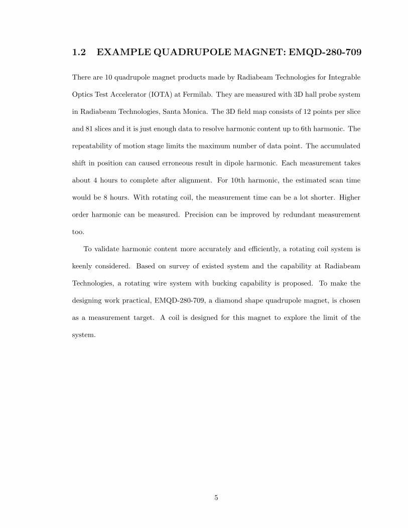
1.2 EXAMPLE QUADRUPOLEMAGNET: EMQD-280-709
There are 10 quadrupole magnet products made by Radiabeam Technologies for Integrable
Optics Test Accelerator (IOTA) at Fermilab. They are measured with 3D hall probe system
in Radiabeam Technologies, Santa Monica. The 3D field map consists of 12 points per slice
and 81 slices and it is just enough data to resolve harmonic content up to 6th harmonic. The
repeatability of motion stage limits the maximum number of data point. The accumulated
shift in position can caused erroneous result in dipole harmonic. Each measurement takes
about 4 hours to complete after alignment. For 10th harmonic, the estimated scan time
would be 8 hours. With rotating coil, the measurement time can be a lot shorter. Higher
order harmonic can be measured. Precision can be improved by redundant measurement
too.
To validate harmonic content more accurately and efficiently, a rotating coil system is
keenly considered. Based on survey of existed system and the capability at Radiabeam
Technologies, a rotating wire system with bucking capability is proposed. To make the
designing work practical, EMQD-280-709, a diamond shape quadrupole magnet, is chosen
as a measurement target. A coil is designed for this magnet to explore the limit of the
system.
5
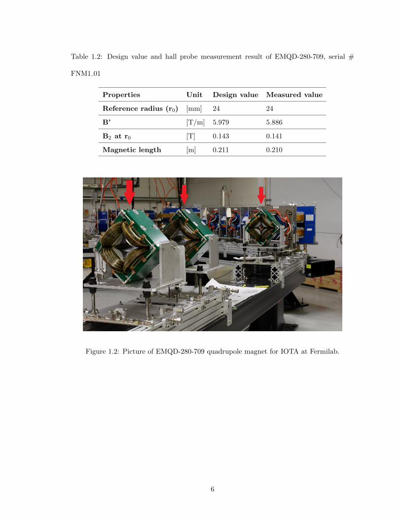
Table 1.2: Design value and hall probe measurement result of EMQD-280-709, serial #
FNM1 01
Properties Unit Design value Measured value
Reference radius (r0) [mm] 24 24
B’ [T/m] 5.979 5.886
B2 at r0 [T] 0.143 0.141
Magnetic length [m] 0.211 0.210
Figure 1.2: Picture of EMQD-280-709 quadrupole magnet for IOTA at Fermilab.
6
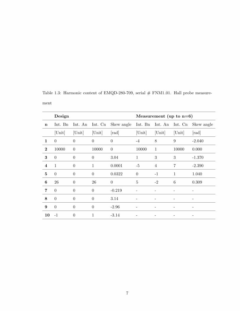
Table 1.3: Harmonic content of EMQD-280-709, serial # FNM1 01. Hall probe measure-
ment
Design Measurement (up to n=6)
n Int. Bn Int. An Int. Cn Skew angle Int. Bn Int. An Int. Cn Skew angle
[Unit] [Unit] [Unit] [rad] [Unit] [Unit] [Unit] [rad]
1 0 0 0 0 -4 8 9 -2.040
2 10000 0 10000 0 10000 1 10000 0.000
3 0 0 0 3.04 1 3 3 -1.370
4 1 0 1 0.0001 -5 4 7 -2.390
5 0 0 0 0.0322 0 -1 1 1.040
6 26 0 26 0 5 -2 6 0.309
7 0 0 0 -0.219 - - - -
8 0 0 0 3.14 - - - -
9 0 0 0 -2.96 - - - -
10 -1 0 1 -3.14 - - - -
7

CHAPTER 2
TECHNOLOGY SURVEY OF
ROTATING COIL METHOD
There are many variations of rotating coil method due to improvement of data acquisition
method and coil production precision. Table 2.1 shows some rotating coil system design
and their measurement specification. Four systems are discussed based on author’s inter-
est. The coil design, bucking capability, accuracy, and repeatability are based on available
publications. [3] [4] [5] [6] [7]
Table 2.1: List of rotating coil system, coil design, bucking, accuracy, and repeatability
based available publications.
Facility Coil design Bucking Accuracy Repeatability(1 sigma)
[unit] [ppm]
BNL 5-Tangential 1st, 2nd <5(before calibration) <26 (up to n=3)
CERN Tangential 1st 0.41(dipole only) 100 (dipole only)
Fermilab* Radial (PCB) 1st, 2nd - 20 (up to n=7)
ANL Radial (Wire) None 0.5 -
*Collaboration work among Fermilab, CERN, and PSI [8]
8

2.1 TANGENTIAL COIL AT BNL, DIGITAL BUCKING
Brookhaven national laboratory (BNL) has tangential coil with traditional winding. How-
ever, each coil is digitized by separated channels. The signal can be manipulated by a
bucking ratio before bucking applies. This extra freedom allows the sensitivity for each coil
to be any number as long as the signal to noise ratio is decent enough. The beauty is that
coil geometry and number of turns can be chosen at any workable combination.
In this merit, BNL comes up with a 5-tangential coil for RHIC quadrupoles and an
upgraded 9-Tangential coil. All coils are wound on the groove of G-10 cylinder with a
maximum of only 36 turns. The 5-tangential coil can measure harmonics from dipole to
12-pole except Octupole [9], with active dipole and quadrupole bucking. The 9-tangential
coil can measure all harmonic, with active bucking up to any three harmonic [10].
Figure 2.1: BNL 5-Tangential coil winding diagram [9] (Left). BNL 9-Tangential coil wind-
ing diagram [10] (Right)
9

Figure 2.2: BNL 5-Tangential coil during calibration. [3]
2.2 ROTATING COIL FIELD MAPPER AT CERN
Traditional rotating coil requires straight through access. For access restricted magnets,
say 90 degree bending dipole, the only applicable measurement technique is hall probe.
However, hall probe in general has relatively worse accuracy. Therefore, a proof-of-principle
field mapper rotating coil is developed at CERN for local field measurement. The rotating
coil probe itself is calibrated to a reference dipole. The accuracy before calibration is 0.41
unit. The fringe field measurement has accuracy of 2%(worst case) between the mapper
and hall probe measurement [4].
10
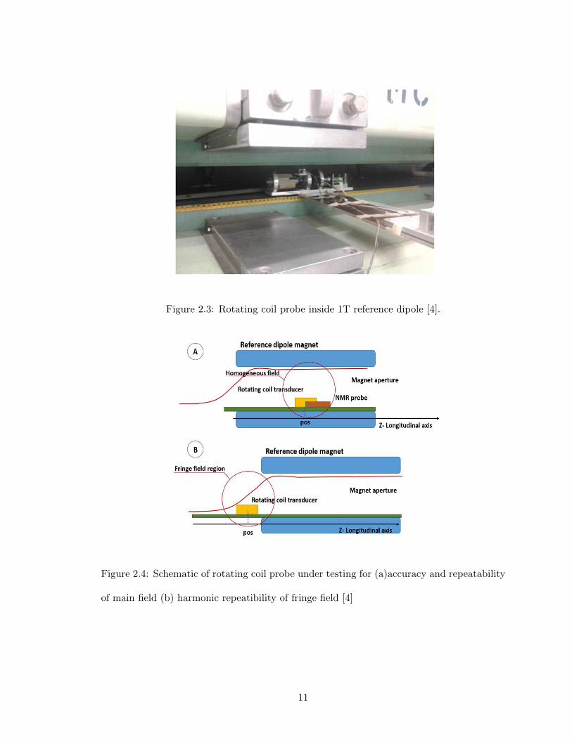
Figure 2.3: Rotating coil probe inside 1T reference dipole [4].
Figure 2.4: Schematic of rotating coil probe under testing for (a)accuracy and repeatability
of main field (b) harmonic repeatibility of fringe field [4]
11
2.3 PCB COILS BY FERMILAB, CERN, AND PSI COL-
LABORATION
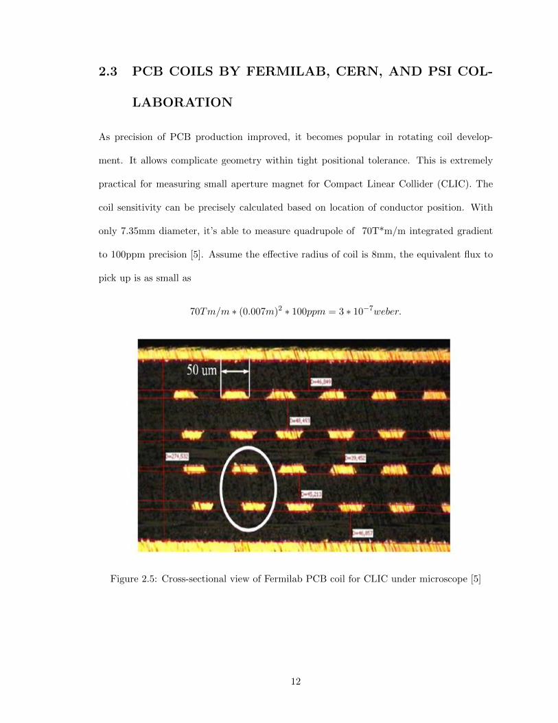
As precision of PCB production improved, it becomes popular in rotating coil develop-
ment. It allows complicate geometry within tight positional tolerance. This is extremely
practical for measuring small aperture magnet for Compact Linear Collider (CLIC). The
coil sensitivity can be precisely calculated based on location of conductor position. With
only 7.35mm diameter, it’s able to measure quadrupole of 70T*m/m integrated gradient
to 100ppm precision [5]. Assume the effective radius of coil is 8mm, the equivalent flux to
pick up is as small as
70Tm/m ∗ (0.007m)2 ∗ 100ppm = 3 ∗ 10−7weber.
Figure 2.5: Cross-sectional view of Fermilab PCB coil for CLIC under microscope [5]
12
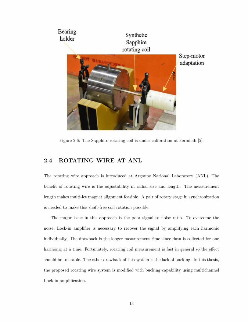
Figure 2.6: The Sapphire rotating coil is under calibration at Fermilab [5].
2.4 ROTATING WIRE AT ANL
The rotating wire approach is introduced at Argonne National Laboratory (ANL). The
benefit of rotating wire is the adjustability in radial size and length. The measurement
length makes multi-let magnet alignment feasible. A pair of rotary stage in synchronization
is needed to make this shaft-free coil rotation possible.
The major issue in this approach is the poor signal to noise ratio. To overcome the
noise, Lock-in amplifier is necessary to recover the signal by amplifying each harmonic
individually. The drawback is the longer measurement time since data is collected for one
harmonic at a time. Fortunately, rotating coil measurement is fast in general so the effect
should be tolerable. The other drawback of this system is the lack of bucking. In this thesis,
the proposed rotating wire system is modified with bucking capability using multichannel
Lock-in amplification.
13
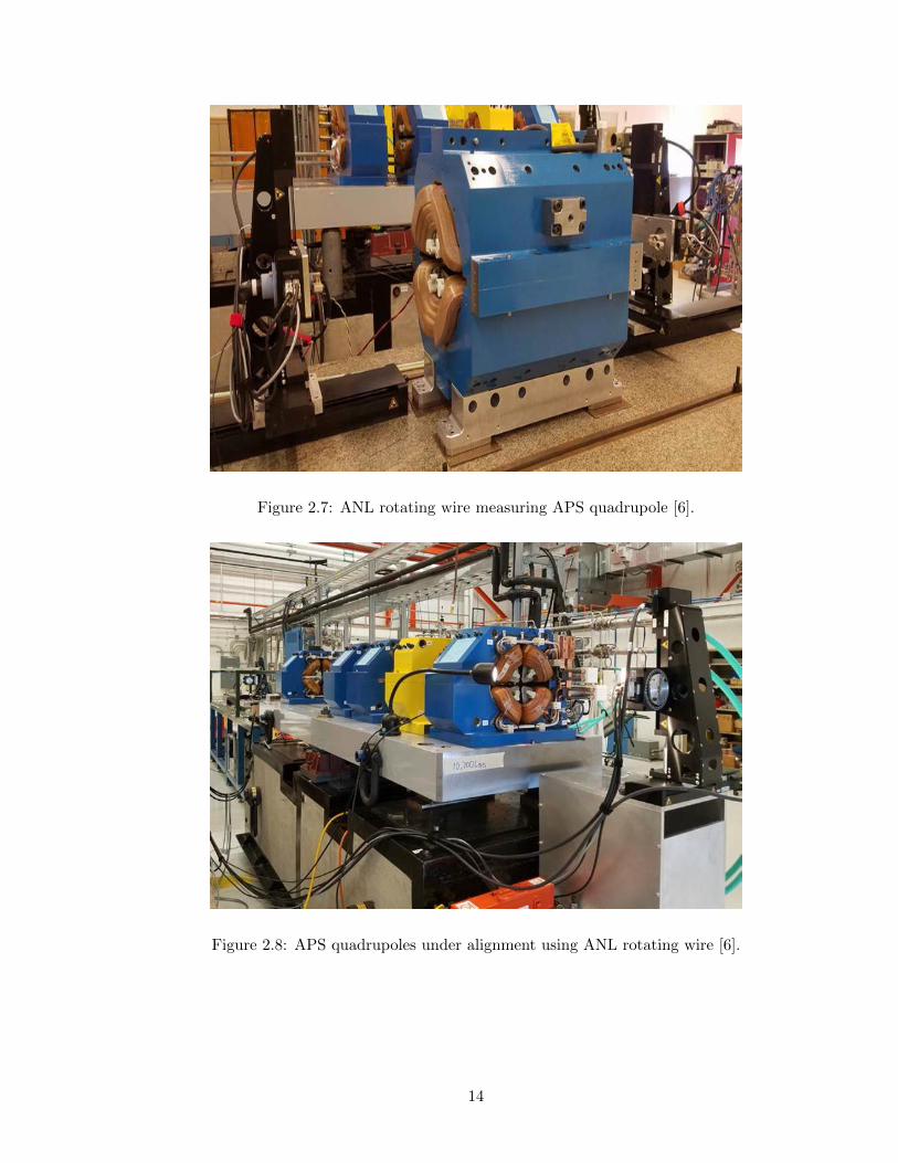
Figure 2.7: ANL rotating wire measuring APS quadrupole [6].
Figure 2.8: APS quadrupoles under alignment using ANL rotating wire [6].
14

CHAPTER 3
THEORY
3.1 MAGNETIC MULTIPOLE IN CYLINDRICAL COOR-
DINATE
In a region free of current or magnetic material, the second and forth Maxwell equation can
be written as:
∇ · ~B = 0 (3.1)
∇× ~B = 0 (3.2)
Magnetic field satisfied equation 3.2 can be written as gradient of scalar potential:
~B = −∇F (3.3)
Combined Equation 3.1 and Equation 3.3, we have the Laplace equation for magnetic
potential:
∇2F = 0 (3.4)
The solution is expressed in either Cartesian or cylindrical coordinate, where the z axis is
parallel to beam trajectory. In two dimension (transverse direction), Equation 3.4 becomes:
∂2F
∂r2+
1
r
∂F
∂r+
1
r2
∂2F
∂θ2= 0 (3.5)
15
Using separation of variable, the general solution of scalar potential is:
F (r, θ) =∑n=1
rn [bnsin (nθ) + ancos(nθ)] (3.6)
where bnand an are arbitral coefficient to be found out. From Equation 3.3, the magnetic
field cylindrical components in 2D are derived:
Br (r, θ) = −∂F∂r
= −∑n=1
nrn−1 [bnsin (nθ) + ancos (nθ) ] (3.7)
Bθ (r, θ) = −1
r
∂F
∂θ= −
∑n=1
nrn−1[bncos (nθ) − ansin(nθ)] (3.8)
Using rotation matrix, the Cartesian components is derived as:
Bx (r, θ) = −∑n=1
nrn−1[bnsin ((n− 1) θ) + ancos ((n− 1) θ) ] (3.9)
By (r, θ) = −∑n=1
nrn−1[bncos ((n− 1) θ) − ansin ((n− 1) θ) ] (3.10)
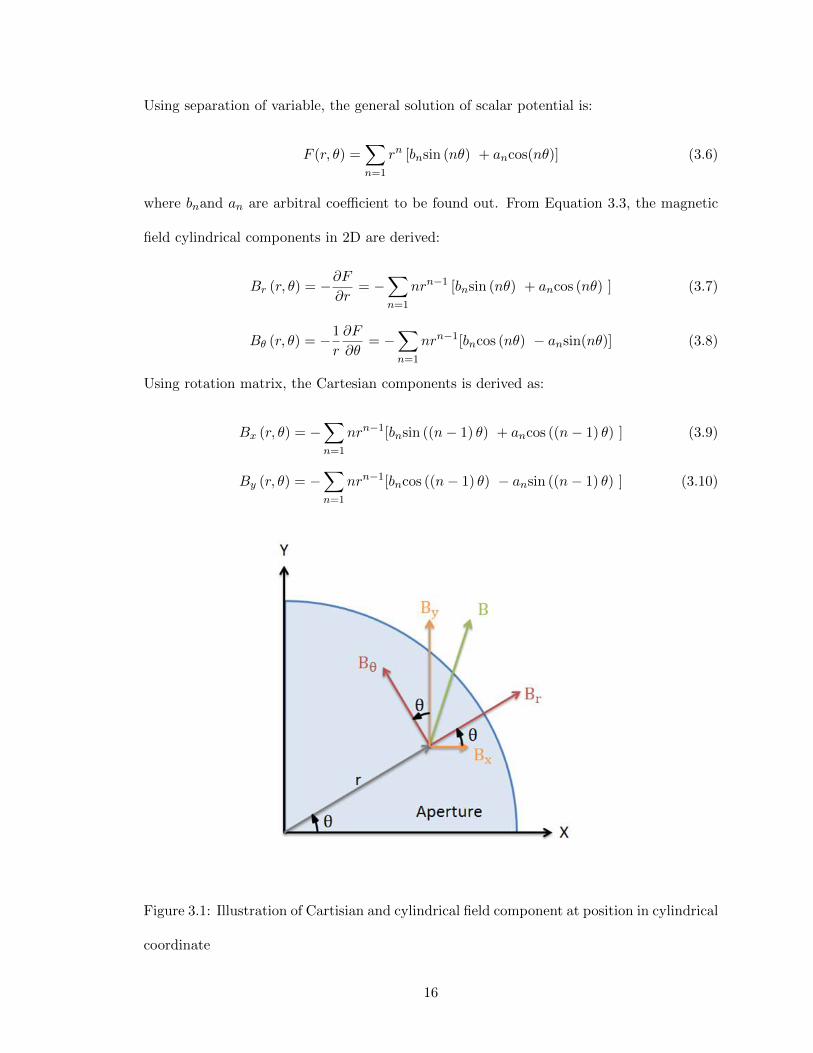
Figure 3.1: Illustration of Cartisian and cylindrical field component at position in cylindrical
coordinate
16

The LHS of Equation 7 and Equation 8 has unit of field while coefficient bnand anhas unit
of fielddistance n−1 . To make coefficients of different order comparable to each other, a new term
is introduced to absorb the dependency of rn−1. Bn(r)
An(r)
= −nrn−1
bn
an
(3.11)
where Bn(r) and An(r) are magnitude of field at radial position r. Bn and An are in the unit
of field (Tesla or Gauss). For clarification, reader should not get confused with coefficient
Bn versus field component Bx, By, Br, and Bθ. The magnitude of field at different radial
position can be written in terms of magnitude of field at a reference radius r0.
Bn (r) =
(r
r0
)n−1
Bn
(r0) (3.12)
Br(r, θ) =∑n=1
(r
r0
)n−1
[Bn(r0) sin (nθ) +An(r0) cos(nθ)] (3.13)
Bθ(r, θ) =∑n=1
(r
r0
)n−1
[Bn(r0) cos (nθ) −An(r0) sin(nθ)] (3.14)
For simplicity, Bn and An are used to stand for Bn(r0) and An(r0), as we keep in mind that
they are the harmonic coefficient acquired at reference radius r0. We acquire the multipole
expansion form in cylindrical coordinate:
Br(r, θ) =∑n=1
(r
r0
)n−1
[Bnsin (nθ) +Ancos(nθ)] (3.15)
Bθ(r, θ) =∑n=1
(r
r0
)n−1
[Bncos (nθ) −Ansin(nθ)] (3.16)
Using rotation matrix and simplify the sinusoidal functions, the Cartesian field component
as function of r and θ can be acquired:
Bx(r, θ) =∑n=1
(r
r0
)n−1
[Bnsin ((n− 1) θ) +Ancos((n− 1)θ)] (3.17)
By(r, θ) =∑n=1
(r
r0
)n−1
[Bncos ((n− 1) θ) −Ansin((n− 1)θ)] (3.18)
17
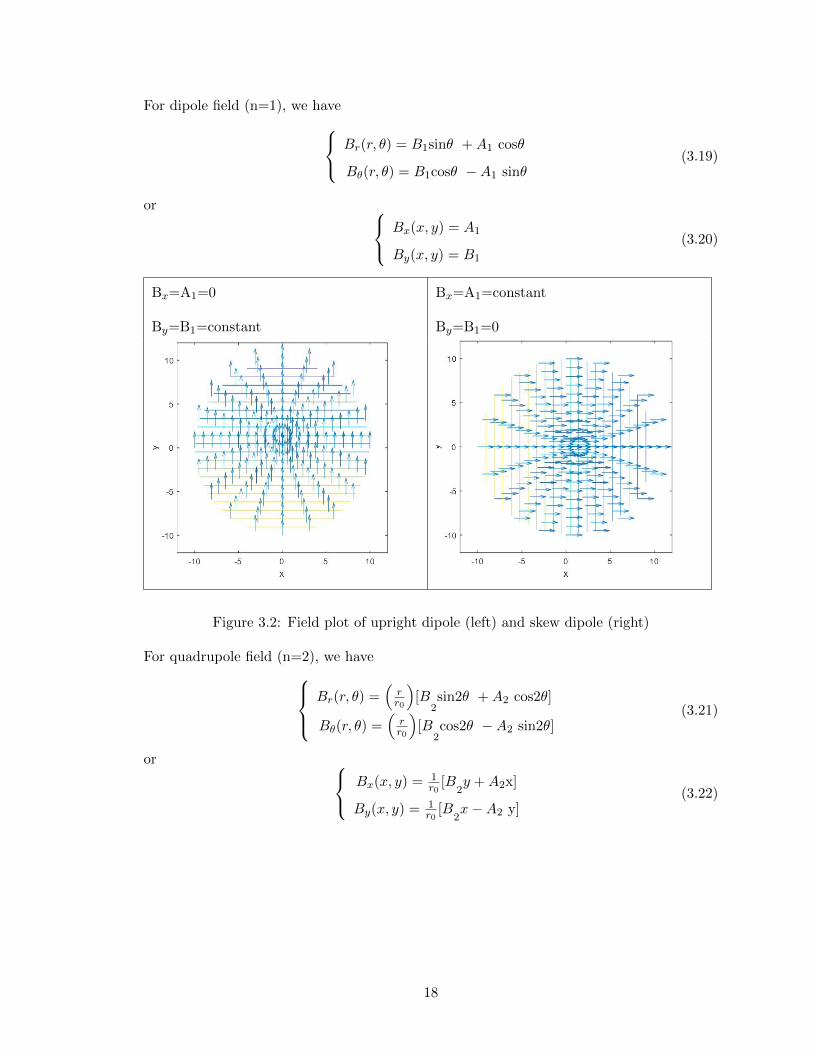
For dipole field (n=1), we have Br(r, θ) = B1sinθ +A1 cosθ
Bθ(r, θ) = B1cosθ −A1 sinθ(3.19)
or Bx(x, y) = A1
By(x, y) = B1
(3.20)
Bx=A1=0
By=B1=constant
Bx=A1=constant
By=B1=0
Figure 3.2: Field plot of upright dipole (left) and skew dipole (right)
For quadrupole field (n=2), we haveBr(r, θ) =
(rr0
)[B
2sin2θ +A2 cos2θ]
Bθ(r, θ) =(rr0
)[B
2cos2θ −A2 sin2θ]
(3.21)
or Bx(x, y) = 1r0
[B2y +A2x]
By(x, y) = 1r0
[B2x−A2 y]
(3.22)
18
Bx = B2r0y
By = B2r0x
Bx = A2r0x
By = −A2r0y
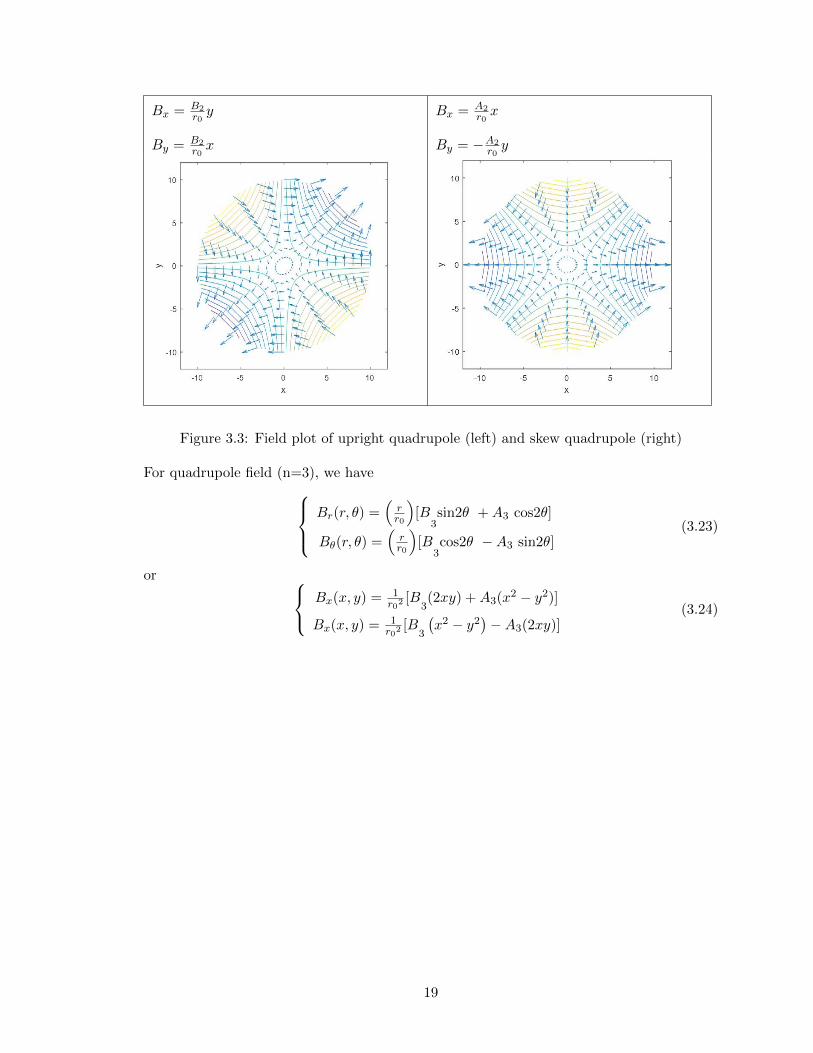
Figure 3.3: Field plot of upright quadrupole (left) and skew quadrupole (right)
For quadrupole field (n=3), we haveBr(r, θ) =
(rr0
)[B
3sin2θ +A3 cos2θ]
Bθ(r, θ) =(rr0
)[B
3cos2θ −A3 sin2θ]
(3.23)
or Bx(x, y) = 1r02
[B3(2xy) +A3(x2 − y2)]
Bx(x, y) = 1r02
[B3
(x2 − y2
)−A3(2xy)]
(3.24)
19

Bx = B3r02
(2xy)
By = B3r02
(x2 − y2
) Bx = A3r02
(x2 − y2
)By = − A3
r02(2xy)
Figure 3.4: Field plot of upright sextupole (left) and skew sextupole (right)
One may notice that the Bn-only multipole field becomes An-only multipole field when it’s
rotated in CW by π2n . The Bn-only field is called “normal” or “upright” field; the An-only
field is called “skew” field. Define Cn =√Bn
2 +An2 to be the magnitude of multipole
coefficient and ϕn = atan(AnBn
)to be the phase angle (also known as skew angle).
Br(r, θ) =∑n=1
(r
r0
)n−1
Cn[cos(ϕn)sin (nθ) + sin(ϕn)cos(nθ)] (3.25)
Bθ(r, θ) =∑n=1
(r
r0
)n−1
Cn[cos(ϕn)cos (nθ) − sin(ϕn)sin(nθ)] (3.26)
Simplifying it, we have the other form of multipole coefficient in terms of Cn and ϕn:
Br(r, θ) =∑n=1
(r
r0
)n−1
Cn[sin (nθ + ϕn) ] (3.27)
Bθ(r, θ) =∑n=1
(r
r0
)n−1
Cn[cos (nθ + ϕn) ] (3.28)
With these multipole coefficients, one can reconstruct the field as function of position and
predict the interaction between magnetic field and charged particle beam.
20
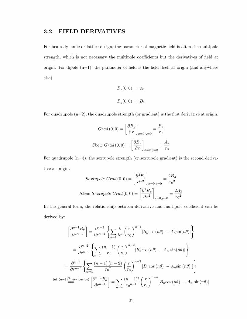
3.2 FIELD DERIVATIVES
For beam dynamic or lattice design, the parameter of magnetic field is often the multipole
strength, which is not necessary the multipole coefficients but the derivatives of field at
origin. For dipole (n=1), the parameter of field is the field itself at origin (and anywhere
else).
Bx(0, 0) = A1
By(0, 0) = B1
For quadrupole (n=2), the quadrupole strength (or gradient) is the first derivative at origin.
Grad (0, 0) =
[∂By∂x
]x=0;y=0
=B2
r0
Skew Grad (0, 0) =
[∂Bx∂x
]x=0;y=0
=A2
r0
For quadrupole (n=3), the sextupole strength (or sextupole gradient) is the second deriva-
tive at origin.
Sextupole Grad (0, 0) =
[∂2By∂x2
]x=0;y=0
=2B3
r02
Skew Sextupole Grad (0, 0) =
[∂2Bx∂x2
]x=0;y=0
=2A3
r02
In the general form, the relationship between derivative and multipole coefficient can be
derived by:
[∂n−1Bθ∂rn−1
]=
∂n−2
∂rn−2
{∑n=1
∂
∂r
(r
r0
)n−1
[Bncos (nθ) −Ansin(nθ)]
}
=∂n−2
∂rn−2
{∑n=2
(n− 1)
r0
(r
r0
)n−2
[Bncos (nθ) −An sin(nθ)]
}
=∂n−3
∂rn−3
{∑n=3
(n− 1) (n− 2)
r02
(r
r0
)n−3
[Bncos (nθ) −Ansin (nθ) ]
}(at (n−1)th derivative)
=⇒[∂n−1Bθ∂rn−1
]=∑n=n
(n− 1)!
r0n−1
(r
r0
)n−n[Bncos (nθ) −An sin(nθ)]
21
=(n− 1)!
r0n−1
[Bncos (nθ) −Ansin (nθ) ]
At origin the (n-1)th field derivative is:
[∂n−1By∂xn−1
]x=0;y=0
=
[∂n−1Bθ∂rn−1
]r=0;θ=0
=(n− 1)!
r0n−1
Bn
Similarly, we can have
[∂n−1Bx∂xn−1
]x=0;y=0
=
[∂n−1Br∂rn−1
]r=0;θ=0
=(n− 1)!
r0n−1
An
Reversing these equations, we get
Bn =r0n−1
(n− 1)!
[∂n−1By∂xn−1
]x=0;y=0
An =r0n−1
(n− 1)!
[∂n−1Bx∂xn−1
]x=0;y=0
(3.29)
Bn and An can be acquired by performing polynomial fit on B vs x data from measure-
ment. However, this approach assumes perfect azimuthal field symmetry, which is highly
unrealistic due to all possible manufacture or assembling errors.
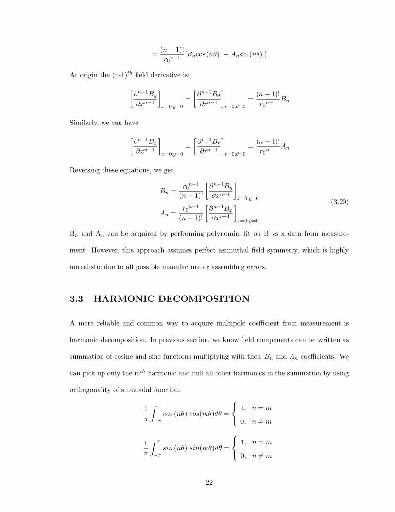
3.3 HARMONIC DECOMPOSITION
A more reliable and common way to acquire multipole coefficient from measurement is
harmonic decomposition. In previous section, we know field components can be written as
summation of cosine and sine functions multiplying with their Bn and An coefficients. We
can pick up only the mth harmonic and null all other harmonics in the summation by using
orthogonality of sinusoidal function.
1
π
∫ π
−πcos (nθ) cos(mθ)dθ =
1, n = m
0, n 6= m
1
π
∫ π
−πsin (nθ) sin(mθ)dθ =
1, n = m
0, n 6= m
22

1
π
∫ π
−πsin (nθ) cos(mθ)dθ = 0
Applying orthogonality between field component Bθ from Equation 3.16 and cos(mθ), the
term bm is picked up and all other terms are left zero.
LHS =1
π
∫ π
−πBθ (r, θ)cos (mθ) dθ
RHS =1
π
∫ π
−π
∑n=1
(r
r0
)n−1
[Bncos (nθ) −Ansin(nθ)]cos(mθ)dθ
=1
π
∫ π
−π
(r
r0
)n−1
Bmcos (mθ) cos (mθ) +∑n=1
1
π
∫ π
−π(other terms)cos(mθ) dθ
=
(r
r0
)n−1
Bm
∫ π
−πcos (mθ) cos (mθ) +
∑n=1
0 =
(r
r0
)n−1
Bm
If we acquire field data only at r=r0 , we have:
Bm =
[1
π
∫ π
−πBθ (r0, θ)cos(mθ)dθ
]
Similarly, we can acquire Am
Am = −[
1
π
∫ π
−πBθ (r0, θ)sin(mθ)dθ
]
The relationship between individual multipole coefficient and field component becomes:
Bm =1
π
∫ π
−πBθ (r0, θ)cos (mθ) dθ =
1
π
∫ π
−πBr (r0, θ)sin(mθ)dθ (3.30)
Am = − 1
π
∫ π
−πBθ (r0, θ)sin (mθ) dθ =
1
π
∫ π
−πBr (r0, θ)cos(mθ)dθ (3.31)
In measurement, a complete and unbiased harmonic analysis requires the field vs position
data of at least one circle, sampling with azimuthal symmetry.
3.4 FIELD QUALITY
The benefit of expressing the multipole coefficient of all order in the same unit is that they
can be normalized to the primary multipole [11] [12]. The normalized multipole coefficients
23
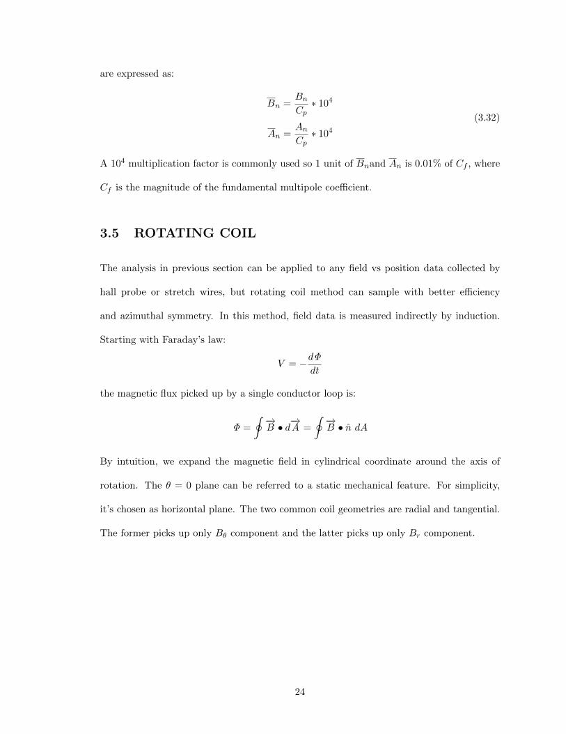
are expressed as:
Bn =BnCp∗ 104
An =AnCp∗ 104
(3.32)
A 104 multiplication factor is commonly used so 1 unit of Bnand An is 0.01% of Cf , where
Cf is the magnitude of the fundamental multipole coefficient.
3.5 ROTATING COIL
The analysis in previous section can be applied to any field vs position data collected by
hall probe or stretch wires, but rotating coil method can sample with better efficiency
and azimuthal symmetry. In this method, field data is measured indirectly by induction.
Starting with Faraday’s law:
V = −dΦ
dt
the magnetic flux picked up by a single conductor loop is:
Φ =
∮ −→B • d
−→A =
∮ −→B • n̂ dA
By intuition, we expand the magnetic field in cylindrical coordinate around the axis of
rotation. The θ = 0 plane can be referred to a static mechanical feature. For simplicity,
it’s chosen as horizontal plane. The two common coil geometries are radial and tangential.
The former picks up only Bθ component and the latter picks up only Br component.
24

3.5.1 RADIAL COIL
Figure 3.5: Axial view of radial coil
Since radial coil is always perpendicular to Bθ, flux of radial coil at angle θ is:
Φ(θ) =
∮Bθ(θ) dA
=
∫ r2
r1
∫Bθ(θ)dzdr
Define L as magnetic length such that∫Bθdz = BθL, the function becomes
Φ(θ) =
∫ r2
r1L∑n=1
(r
r0
)n−1
[Bncos (nθ) −Ansin(nθ)]dr
=∑n=1
Lr0
n
[(r2
r0
)n−(r1
r0
)n][Bncos (nθ) −An sin(nθ)]
=∑n=1
Kn [Bncos (nθ) −Ansin (nθ) ]
Kn = Lr0n
[(r2r0
)n−(r1r0
)n]is known as the sensitivity factor, which only depends on coil
geometry. When r1=0 in radial coil, the returning conductor is on the axis of rotation and
Kn becomes Lr0n
(rr0
)n.
25
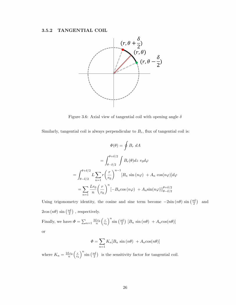
3.5.2 TANGENTIAL COIL
Figure 3.6: Axial view of tangential coil with opening angle δ
Similarly, tangential coil is always perpendicular to Br, flux of tangential coil is:
Φ(θ) =
∮Br dA
=
∫ θ+δ/2
θ−δ/2
∫Br(θ)dz r0dϕ
=
∫ θ+δ/2
θ−δ/2L∑n=1
r
(r
r0
)n−1
[Bn sin (nϕ) +An cos(nϕ)]dϕ
=∑n=1
Lr0
n
(r
r0
)n[−Bncos (nϕ) +Ansin(nϕ)]|θ+δ/2θ−δ/2
Using trigonometry identity, the cosine and sine term become −2sin (nθ) sin(nδ2
)and
2cos (nθ) sin(nδ2
), respectively.
Finally, we have:Φ =∑
n=12Lr0n
(rr0
)nsin(nδ2
)[Bn sin (nθ) +Ancos(nθ)]
or
Φ =∑n=1
Kn[Bn sin (nθ) +Ancos(nθ)]
where Kn = 2Lr0n
(rr0
)nsin(nδ2
)is the sensitivity factor for tangential coil.
26

3.5.3 SINGLE WIRE AND GENERAL COIL FORM
When δ = πn in tangential coil, Kn reaches maximum and is twice of Kn for single wire.
Here we take quadrupole (n=2) as example. In figure 3.7 (left), tangent coil of π2 open angle
is exposed to magnetic flux of top right quadrant when it’s at θ = π4 . The figure 3.7 (right)
shows four tangent coils with different path. They all have same flux exposure as long as
the axial conductor segments are at the same location.
Figure 3.7: The π2 tangential coil of “quarter-circle” geometry (left). The π
2 tangential coil
when the vertex are connected by four different paths (right). All these coils have the same
flux exposure.
The L-shape path’s connection at origin can break into two segments. When a pair vertex
(red) and vertex (green) node are added at origin, two radial coils are formed.
27
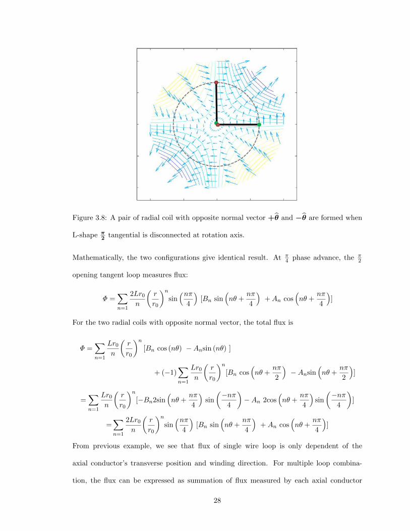
Figure 3.8: A pair of radial coil with opposite normal vector +θ̂ and −θ̂ are formed when
L-shape π2 tangential is disconnected at rotation axis.
Mathematically, the two configurations give identical result. At π4 phase advance, the π
2
opening tangent loop measures flux:
Φ =∑n=1
2Lr0
n
(r
r0
)nsin(nπ
4
)[Bn sin
(nθ +
nπ
4
)+An cos
(nθ +
nπ
4
)]
For the two radial coils with opposite normal vector, the total flux is
Φ =∑n=1
Lr0
n
(r
r0
)n[Bn cos (nθ) −Ansin (nθ) ]
+ (−1)∑n=1
Lr0
n
(r
r0
)n[Bn cos
(nθ +
nπ
2
)−Ansin
(nθ +
nπ
2
)]
=∑n=1
Lr0
n
(r
r0
)n[−Bn2sin
(nθ +
nπ
4
)sin
(−nπ
4
)−An 2cos
(nθ +
nπ
4
)sin
(−nπ
4
)]
=∑n=1
2Lr0
n
(r
r0
)nsin(nπ
4
)[Bn sin
(nθ +
nπ
4
)+An cos
(nθ +
nπ
4
)]
From previous example, we see that flux of single wire loop is only dependent of the
axial conductor’s transverse position and winding direction. For multiple loop combina-
tion, the flux can be expressed as summation of flux measured by each axial conductor
28
with proper sign. To make the derivation simpler, complex variable is introduced. First
Bncos (nθ) − Ansin (nθ) is rewritten as Re {[Bn + iAn] [cos (nθ) + isin (nθ) ]} and it be-
comes Re{
[Bn + iAn] einθ}
. The flux picked up by single rotating wire at position angle
θ + α is:
Re
{Lr0
n
(r
r0
)n(Bn + iAn) ein(θ+α)
}= Re
{Lr0
n
(reiα
r0
)n(Bn + iAn) einθ
}= Re
{Kn (Bn + iAn) einθ
}where the new sensitivity factor is Kn = Lr0
n
(reiα
r0
)n. For coil constructed by multiple axial
segments at different location with alternating winding direction, we get:
Kn =
N∑j
Lr0
n
(r
r0
)neinαj (−1)j (3.33)
This general form for flux of an arbitrary coil is [13]:
Φ (θ) = Re
{∑n=1
Kn (Bn + iAn) einθ
}(3.34)
3.5.4 MORGAN COIL
Morgen coil [14] [15] use special winding for particular harmonic order. For mth order
harmonic, ”2m” axial-direction conductors are located equally spaced by πm , with alternating
winding direction. When nth order harmonic is measured by mth order Morgan coil, αj =(jπm
). Therefore, ein(
jπm )(−1)j = eiπj(1+ n
m). This value is 1 when n = m, 3m, 5m, . . . ,etc.
Morgan coil is n times sensitive to its fundamental harmonic and the allowed harmonic with
the peak Kn = Lr0
(rr0
)n. In these cases, flux measured by each wire is in phase. For other
harmonic, the sensitivity is zero.
Kn =Lr0
n
(r
r0
)n 2m∑j
eiπj(1+ nm
) =
Lr0n
(rr0
)n∗ 2m, n = m, 3m, 5m. . .
0, n = else
29

Since each Morgan coil only measures its own fundamental harmonic, many of them are
required to measure a magnet up to sufficient harmonic order. For dipole magnet, it may
be reasonable to 5th order. For quadrupole, it may be necessary to measure harmonic up to
10th order. Space limit on winding fixture is the challenging especially for small aperture
measurement. The angular position of each coil needs careful measurement with respect to
the reference feature for θ = 0 plane.
Figure 3.9: Morgan coil for first, second and third order harmonic. Black and red vertex
represents conductor wound in opposite direction.
3.6 SIGNAL PROCESSING
The coil measures signal in voltage waveform:
V (t) = −dΦ(ωt)
dt
Since inconsistent rotation speed ω can affect signal strength, it’s more common to analyze
the signal after time integration.
30

Figure 3.10: Asymmetric data per revolution caused by inconsistent rotation speed cause if
sampling is time-based (left). Symmetric data collected when angle-based sampling is used
(right).
During rotation, rotary encoder generates discrete signal when one unit of rotation δθ is
executed. Then the integrator runs its build-in timer and stamp the time based on encoder
signal. After integration, the discrete signal becomes
V s [θk] =k∑i=0
V [θi] δt [θi] = −Φ[θk] (3.35)
θk = kδθ is the angular position of coil. V [θi] is the voltage signal sampled at angular
position θi. δt [θi]is the lapse time between adjacent angular position. N = 2πδθ is the
number of sampling point for one cycle. Applying Fast Fourier Transformation on both
side of equation, we get:
FFT (V s)n = −∑n=1
Kn (Bn + iAn)
N∑k=1
einθke−i2πnkNs
= −∑n=1
Kn (Bn + iAn)
N∑k=1
1
= −N∑n=1
Kn (Bn + iAn)
31

The harmonic coefficients in terms of integrated voltage signal are:
Bn = −Re{FFT (V s)n
NKn
}An = −Im
{FFT (V s)n
NKn
}Cn =
∣∣∣∣FFT (V s)nNKn
∣∣∣∣ϕn = atan
(AnBn
)(3.36)
Where FFT (V s)[n] stands for the nth data of FFT signal. Notice that Kn is complex
number written as:
Kn =∑j
Lr0
n
(r
r0
)neinαj (−1)j
The sensitivity for the four coil types mention in previous section are presented here:
Radial coil:
Kn =Lr0
n
[(r2
r0
)n−(r1
r0
)n](3.37)
Tangential coil:
Kn = −i2Lr0
n
(r
r0
)nsin
(nδ
2
)(3.38)
Single wire:
Kn =Lr0
n
(r
r0
)n(3.39)
Morgan coil of mth harmonic:
Kn =
2mLr0n
(rr0
)n, n = m, 3m, 5m. . .
0, n = else(3.40)
3.7 ERROR PROPAGATION
The limiting factors of accuracy and precision in rotating coil method are dynamic posi-
tion, signal resolution, and false signal. They are linked directly to data acquisition, data
transmission noises, rotation speed consistency, and coil geometry.
Cn =
∣∣∣∣FFT (V s)nNKn
∣∣∣∣32
∆CnCn
=
√(∆V oltage
Cn
)2
+
(∆time
Cn
)2
+
(∆θ
Cn
)2
+
(∆Kn
Cn
)2
(3.41)
The first term depends on the ADC accuracy and the noise during data transmission.
The second term depends on the time stamping process inside integrator. The third term
depends on the rotation of coil in lab frame. The last term depends on the coil geometry
and vibration in coil frame. If Voltage data is analyzed instead, the nth harmonic and error
becomes:
Cn =
∣∣∣∣FFT (V )nωNKn
∣∣∣∣∆CnCn
=
√(∆V oltage
Cn
)2
+
(∆ω
ω
)2
+
(∆θ
Cn
)2
+
(∆Kn
Cn
)2
(3.42)
The only difference is that the error in integration time is replaced by error in rotation
speed error.
3.7.1 ERROR AND NOISE IN DAQ AND DATA TRANSMISSION
There are three portion of error in voltage signal digitization: Gain error, offset error, and
noise. The first two errors limit the accuracy and the last error limits the resolution and
precision. The gain error and offset error are temperature dependent and can increase in
time after each calibration. Therefore, it’s important to operate the device in a temperature
controlled environment and calibrate it in regular basis. The noise is often expressed in
root mean square form. For high confidence, the peak to peak noise error use 3-sigma. The
value of error and noise are also dependent to sampling rate and input scale. Noise in data
transmission is different from digitizing noise. The source of this noise can be electrical
noise from nearby hardware [15] (for example, power supply, computer, motors,. . . , etc.)
and the signal carrier (slip ring, solder joint, and cable). This type of noise has specific
frequency that can be dependent to the measurement. For example, slip ring noise is
coupled with rotation. The noise from function generator in pulse magnet is directly related
33
to measurement too. The expression for systematic voltage signal error is:
∆Vgain + ∆Voffset + ∆Vsystem noise
= V in[θi] ∗ gain error + ∆Voffset + ∆Vsystem noise[θi]
The offset error has no contribution after FFT. However, if signal strength is close to
measurement range of DAQ, this offset error may cause signal loss when overloaded signal
gets truncated. The third part of error is noise from environment and signal carrier. The
noise from DAQ is excluded in this calculation for systematic error because it’s random
noise. The error contribution due to voltage signal error is derived as:
∆V oltage
Cn=
1
FFT (V s)nFFT
{k∑i=0
(Vin[θi] ∗ gain error + ∆Vsystem noise[θi]) δt[θi]
}
= gain error +FFT (∆Vsystem noise)n ∗Rotation period
FFT (V s)n(3.43)
The gain error can be found in DAQ specification. The spectrum of system noise needs to
be evaluated by background measurement.
The resolution of voltage signal depends on signal to noise ratio. For a resolvable signal,
the SNR need to be at least greater than two. Therefore the minimum voltage signal of nth
harmonic is:
FFT (V )n ≥ N ∗ 2 ∗ (3σV )
,where σV is the noise of DAQ. Notice that FFT magnifies the result by N times. This
N factor needs to be compensated before comparing it with time-domain magnitude. The
minimum resolvable harmonic strength becomes:
min(|Cn|) =
∣∣∣∣2 ∗ (3σV )
ωKn
∣∣∣∣,where ω is the average rotation speed.
For example, if σV = 1uV , ω = 1Hz, and K6 = 0.2, the minimum resolvable 6th harmonic
|C6| would be ∼5 uT. If the fundamental harmonic, say quadrupole, is 0.05T, the ratio
34

between 6th and 2nd harmonic is 1 unit or 100 ppm. This is measurement precision for 6th
harmonic by DAQ, assuming all other noises are zero. When evaluating the final precision
of system, all source of noise will contribution to the numerator.
The error in voltage signal caused by inconsistent rotation speed is discussed in next section
because it’s an error due to dynamic error.
3.7.2 ERROR AND NOISE IN INTEGRATION TIME
There are two errors in signal involves with time. The first error is due to inconsistent
rotation speed. The effect to voltage signal strength can be removed by time integration.
If integration happens after digitization, there will be numerical integration error. For
periodic function, trapezoidal method has really high accuracy for small numbers of point
per harmonic cycle [16]. The second error comes from the minimum step and accuracy in
DAQ timer. Because digital trigger is used, the time accuracy of voltage signal can only be
as good as the trigger pulse width. The error contribution of error in time is:
∆time
Cn=
1
FFT (V s)nFFT
{k∑i
V [θi] ∆ttrigger
}
=1
FFT (V s)nFFT
{k∑i
V [θi] ∗ δt[θi]
}∆ttriggerδt[θi]
≈ ∆ttriggerT/N
(3.44)
Notice that time error ∆ttrigger is additional to correct time interval δt[θi]. Since rotation
speed is not constant,∑Ns
k V [θi] need to multiply with proper δt[θi] to be zero. The residual
signal due to ∆ttrigger will be observed as vertical drift on voltage-time signal. T/N is the
rotation period divided by number of encoder pulses. The other possible error happens
when the encoder signal is miss-counted. The consequence is a discontinuity on voltage-
time signal. As we know, discontinuity in signal generates combination of infinite Fourier
series. It will generate a broad band error spectrum to the result signal. Test on encoder
counts needs to be performed on regular basis. If miscounting occurs consistently, the
35
encoder should be replaced. There’s also time error due current sweep time in AC or pulse
magnet but it is not discussed in this thesis.
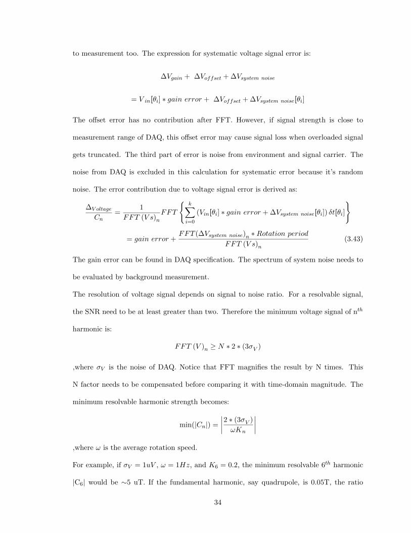
3.7.3 ERROR IN ANGULAR POSITION
The error caused by systematic error ∆θ is simply an angular shift in integrated signal:
∆θ
Cn=
1
FFT (V s)nFFT
k∑j
V [θj ]δt[θj ]ein∆θ
= ein∆θ (3.45)
This ∆θ error exists due to minimum step of δt in time integral. The angular misplacement
of coil is not discussed here but in coil geometry section. When V [θi] δt [θi] is calculated, it
actually represents the average flux portion δΦ at θk + δθ2 position, regardless of integration
method. Therefore the analysis result will be skewed by δθ2 in the direction of rotation.
This error can be reduced by having a higher step resolution encoder. Alternatively, it can
be easily removed by performing a measurement in reversed direction and take the average.
Figure 3.11: Integration fragment V [θi] δt [θi] doesn’t give δΦ [θi] but δΦ[θi+
δθ2
]
36
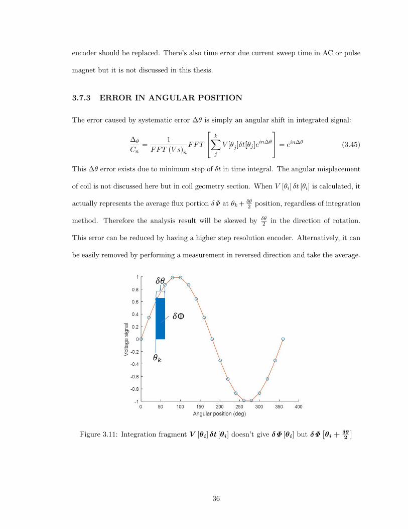
3.7.4 ERROR IN COIL GEOMETRY
The general form for sensitivity of single wire is:
Kn =Lr0
n
(r
r0
)neinα
Both r and α has systematic error ∆r, ∆α and random error σr , σα along z direction.
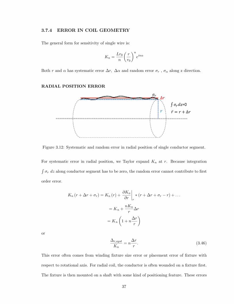
RADIAL POSITION ERROR
Figure 3.12: Systematic and random error in radial position of single conductor segment.
For systematic error in radial position, we Taylor expand Kn at r. Because integration∫σr dz along conductor segment has to be zero, the random error cannot contribute to first
order error.
Kn (r + ∆r + σr) = Kn (r) +∂Kn
∂r
∣∣∣∣r
∗ (r + ∆r + σr − r) + . . .
= Kn +nKn
r∆r
= Kn
(1 + n
∆r
r
)or
∆r,syst
Kn= n
∆r
r. (3.46)
This error often comes from winding fixture size error or placement error of fixture with
respect to rotational axis. For radial coil, the conductor is often wounded on a fixture first.
The fixture is then mounted on a shaft with some kind of positioning feature. These errors
37
in size and position accumulate. Also, the shaft is connected to motor with possible (but
often small) concentricity error. The printed circuit board (PCB) coil would have more
concentricity error if cylindrical shaft is not used. For simplicity, error in angular position
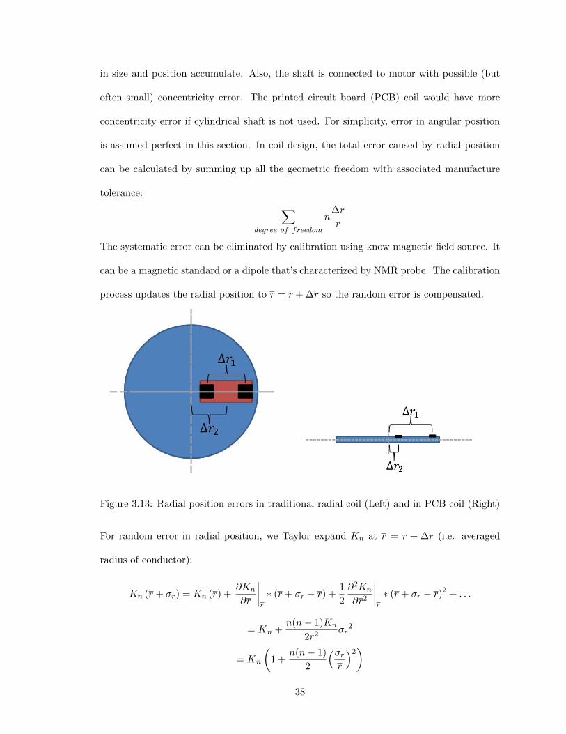
is assumed perfect in this section. In coil design, the total error caused by radial position
can be calculated by summing up all the geometric freedom with associated manufacture
tolerance: ∑degree of freedom
n∆r
r
The systematic error can be eliminated by calibration using know magnetic field source. It
can be a magnetic standard or a dipole that’s characterized by NMR probe. The calibration
process updates the radial position to r = r + ∆r so the random error is compensated.
Figure 3.13: Radial position errors in traditional radial coil (Left) and in PCB coil (Right)
For random error in radial position, we Taylor expand Kn at r = r + ∆r (i.e. averaged
radius of conductor):
Kn (r + σr) = Kn (r) +∂Kn
∂r
∣∣∣∣r
∗ (r + σr − r) +1
2
∂2Kn
∂r2
∣∣∣∣r
∗ (r + σr − r)2 + . . .
= Kn +n(n− 1)Kn
2r2 σr2
= Kn
(1 +
n(n− 1)
2
(σrr
)2)
38

or
∆r,rand
Kn=n(n− 1)
2
(σrr
)2(3.47)
A random error in coil cannot be calibrated but it will attenuated by adding more conductor
segments. Since the segments are electrically connected, the random error spread over the
prolonged conductor length. A coil of ”N” axial segments of conductor should have its
random error drop by factor of 1N .
ANGULAR POSITION ERROR
Figure 3.14: Systematic and random error in angular position of single conductor segment.
Similarly, for systematic error in angular position, we Taylor expand Kn at α:
Kn (α+ ∆α+ σα) = Kn +∂Kn
∂α
∣∣∣∣α
∗ (α+ ∆α+ σα − α) + . . .
= Kn + inKn∆α
= Kn (1 + in∆α)
or
∆α,syst
Kn= in∆α (3.48)
Notice that this error is imaginary so in addition to error in magnitude, it also gives error
in skew angle. The systematic angular error is equivalent to an angular offset with respect
to zero reference. It can be calibrated by a known magnetic field source with known skew
39
angle with respect to the angular reference. Alternatively, we can performed a measurement
reversely and take the average of two measurement data.
Particularly, angular position error is the major manufacture error in tangential coil. The
conductor often wound directly on the rotating shaft. It eliminates one source of error in
assembling. The shaft is machined with notches to accommodate conductors. In this way,
the error in radial position should be well-controlled by natural unless shaft and motor has
concentricity issue. Recall that sensitivity for tangential coil is:
Kn = −i2Lr0
n
(r
r0
)nsin
(nδ
2
)
When two conductor segments have systematic error ∆α1and ∆α2, the systematic error in
opening angle becomes ∆δ = |∆α1 −∆α2|. Taylor expand Kn at δ gives
Kn (δ + ∆δ + σδ) = Kn +∂Kn
∂δ
∣∣∣∣δ
∗ (δ + ∆δ + σδ − δ) + . . .
= Kn +Kn
(n2
)cos
(nδ
2
)∆δ
= Kn
[1 +
(n2
)cos
(nδ
2
)∆δ
]or
∆δ,syst
Kn=(n
2
)cos
(nδ
2
)∆δ (3.49)
The systematic error in angular position for tangential coil is the same as single wire case,
with substitution of ∆α=∆α1+∆α22 .
40

Figure 3.15: Angualr position errors in tangential coil
For random error in angular position, we Taylor expand Kn at α = α + ∆α (i.e. averaged
angle of conductor):
Kn (α+ σα) = Kn +∂Kn
∂α
∣∣∣∣α
∗ (α+ σα − α) +1
2
∂2Kn
∂α2
∣∣∣∣α
∗ (α+ σα − α)2 + . . .
= Kn −n2Knσα
2
2
= Kn
(1− n2
2σα
2
)or
∆α,rand
Kn= −n
2
2σα
2 (3.50)
In the case of tangential coil, the random error is derived by simply substituting σα by σα2
because the length of axial conductor segment is doubled. Therefore we get
∆δ,rand
Kn= −n
2
8σα
2 (3.51)
For coil of N axial conductor segments, the general form of sensitivity error due to positional
error can be calculated by:
|∆Kn| =
√√√√√ N∑
j
∆rj ,syst
2
+
N∑j
∆αj ,syst
2
+
(∆rj ,rand
N
)2
+
(∆αj ,rand
N
)2
41
The error in harmonic content due to sensitivity error is acquired:
∆Kn
Cn=
√√√√√ N∑
j
∆rj ,syst
Kn
2
+
N∑j
∆αj ,syst
Kn
2
+
(∆rj ,rand
NKn
)2
+
(∆αj ,rand
NKn
)2
(3.52)
This formula assumes that errors in radial and angular position are independent. There are
cases when the two error couples. For example, the radial or tangential coil can tilt with
respect to its center of mass. The other example would be the occasion when the shaft
is not concentric to motor axis. Discussion of these special cases can be found in other
paper [17].
3.7.5 COIL VIBRATION
While rotation speed error is removed from the formula of signal strength after time in-
tegration, the vibration triggered by time varying angular velocity can cause fake signal,
especially when the speed varies periodically. With proper choice of rotation speed, hun-
dreds of measurement can be collected within a minutes. The random vibrational error soon
vanishes. The only observable vibrations are systematic and have to be periodic. Although
the vibration can be detected by sensor and measured for frequency, it cannot be eliminated
by calibration.
42
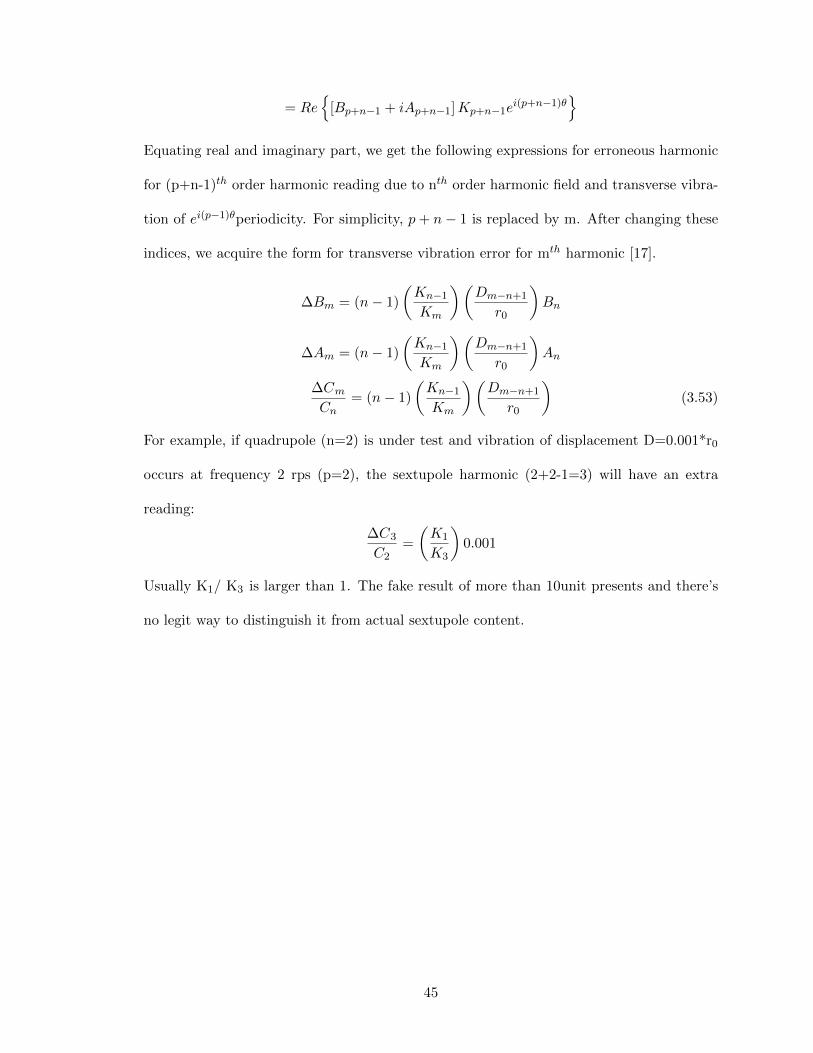
TRANSVERSE VIBRATION
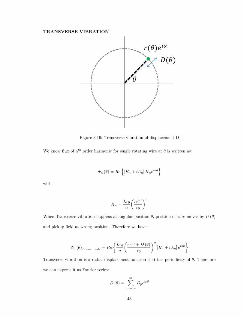
Figure 3.16: Transverse vibration of displacement D
We know flux of nth order harmonic for single rotating wire at θ is written as:
Φn (θ) = Re{
[Bn + iAn]Kneinθ}
with
Kn =Lr0
n
(reiα
r0
)nWhen Transverse vibration happens at angular position θ, position of wire moves by D (θ)
and pickup field at wrong position. Therefore we have:
Φn (θ)Trans. vib. = Re
{Lr0
n
(reiα +D (θ)
r0
)n[Bn + iAn] einθ
}Transverse vibration is a radial displacement function that has periodicity of θ. Therefore
we can express it as Fourier series:
D (θ) =∞∑
p=−∞Dpe
ipθ
43
Before deriving for general form, we need to verify if the expression is valid for trivial
cases. When wire is sensing dipole field, transverse vibration should have no effect on flux
measurement due to dipole field’s uniformity. Mathematically, it means
Φ1 (θ)D = Re
{Lr0
1
(reiα +D (θ)
r0
)1
[B1 + iA1] eiθ
}= Re
{Lr0
1
(reiα
r0
)1
[B1 + iA1] eiθ
}
To satisfy this condition, D(θ)r0eiθ has to be zero all the time, we redefine the vibration as [17]:
D (θ) =
∞∑p=−∞
Dpei(p−1)θ
The derivation becomes:
Φn (θ)D = Re
{Lr0
n
(reiα +D (θ)
r0
)n[Bn + iAn] einθ
}
= Re
{Lr0
n
[(reiα
r0
)n+ n
(reiα
r0
)n−1(D (θ)
r0
)+ . . .
][Bn + iAn] einθ
}
≈ Re
{Lr0
n
[(reiα
r0
)n+ n
n− 1
n− 1
(reiα
r0
)n−1(D (θ)
r0
)][Bn + iAn] einθ
}
= Re
{Kn[Bn + iAn] einθ + (n− 1)Kn−1
(D (θ)
r0
)[Bn + iAn] einθ
}In the end, we get
Φn (θ)D ≈ Φn (θ) +Re
{(n− 1)Kn−1
(D (θ)
r0
)[Bn + iAn] einθ
}The first them is the non-perturbed nth flux. The second term is the erroneous flux ∆Φ
due to transverse vibration. Substituting D (θ) =∑∞−∞Dpe
i(p−1)θ into it, we have
∆Φ = Re
{(n− 1)Kn−1
(∑∞−∞Dpe
i(p−1)θ
r0
)[Bn + iAn] einθ
}
= Re
{(n− 1)Kn−1 [Bn + iAn]
∞∑−∞
Dp
r0ei(p+n−1)θ
}After FFT, the term with ei(p+n−1)θ multiplier will be “deciphered” as the (p+n-
1)th harmonic Φp+n−1. Therefore we have:
Re
{(n− 1)Kn−1 [Bn + iAn]
Dp
r0ei(p+n−1)θ
}= Φp+n−1
44
= Re{
[Bp+n−1 + iAp+n−1]Kp+n−1ei(p+n−1)θ
}Equating real and imaginary part, we get the following expressions for erroneous harmonic
for (p+n-1)th order harmonic reading due to nth order harmonic field and transverse vibra-
tion of ei(p−1)θperiodicity. For simplicity, p+ n− 1 is replaced by m. After changing these
indices, we acquire the form for transverse vibration error for mth harmonic [17].
∆Bm = (n− 1)
(Kn−1
Km
)(Dm−n+1
r0
)Bn
∆Am = (n− 1)
(Kn−1
Km
)(Dm−n+1
r0
)An
∆CmCn
= (n− 1)
(Kn−1
Km
)(Dm−n+1
r0
)(3.53)
For example, if quadrupole (n=2) is under test and vibration of displacement D=0.001*r0
occurs at frequency 2 rps (p=2), the sextupole harmonic (2+2-1=3) will have an extra
reading:
∆C3
C2=
(K1
K3
)0.001
Usually K1/ K3 is larger than 1. The fake result of more than 10unit presents and there’s
no legit way to distinguish it from actual sextupole content.
45
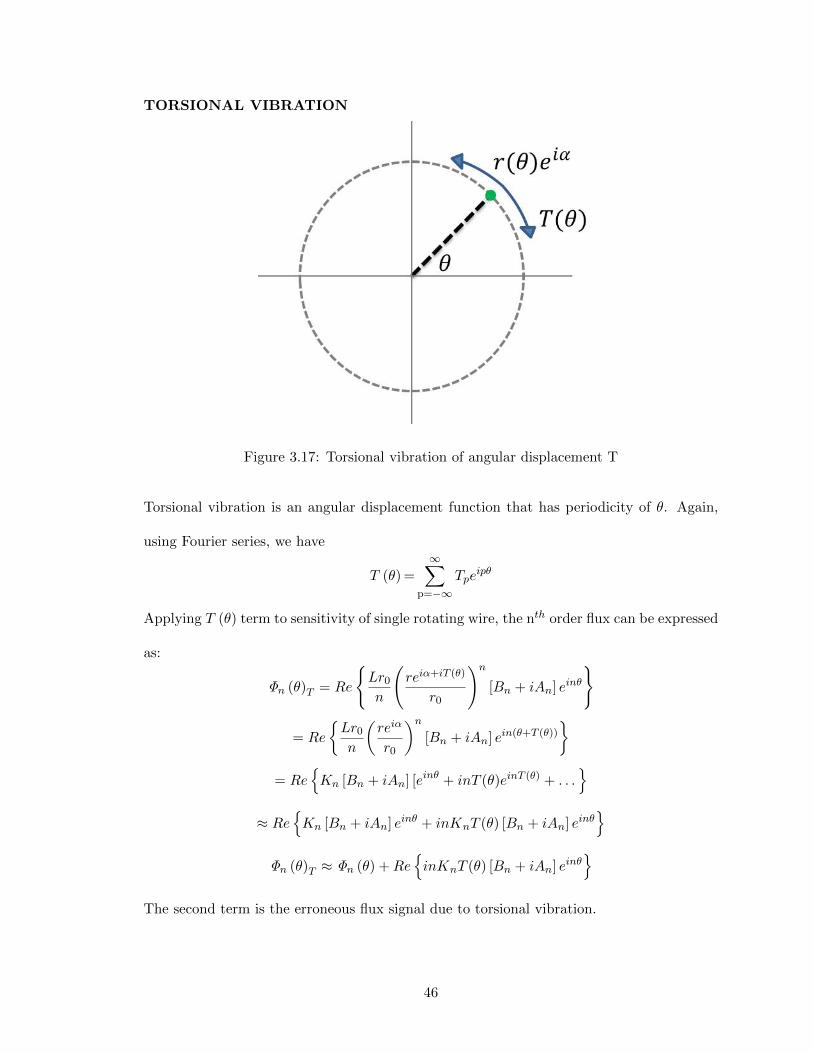
TORSIONAL VIBRATION
Figure 3.17: Torsional vibration of angular displacement T
Torsional vibration is an angular displacement function that has periodicity of θ. Again,
using Fourier series, we have
T (θ) =
∞∑p=−∞
Tpeipθ
Applying T (θ) term to sensitivity of single rotating wire, the nth order flux can be expressed
as:
Φn (θ)T = Re
{Lr0
n
(reiα+iT (θ)
r0
)n[Bn + iAn] einθ
}
= Re
{Lr0
n
(reiα
r0
)n[Bn + iAn] ein(θ+T (θ))
}= Re
{Kn [Bn + iAn] [einθ + inT (θ)einT (θ) + . . .
}≈ Re
{Kn [Bn + iAn] einθ + inKnT (θ) [Bn + iAn] einθ
}Φn (θ)T ≈ Φn (θ) +Re
{inKnT (θ) [Bn + iAn] einθ
}The second term is the erroneous flux signal due to torsional vibration.
46
Substituting T (θ) =∑∞−∞ Tpe
ipθ into it, we have
∆Φ = Re
{inKn
∞∑p=−∞
Tpeipθ [Bn + iAn] einθ
}= Re
{inKn [Bn + iAn]
∞∑p=−∞
Tpei(p+n)θ
}
After FFT, this erroneous signal due to nth order field harmonic and torsional vibration of
eipθ will be “deciphered” as the (p+n)th order harmonic:
Re{inKn [Bn + iAn]Tpe
i(p+n)θ}
= Φp+n (θ) = Re{Kp+n [Bp+n + iAp+n] ei(p+n)θ
}Again, replace p+ n− 1 by m, we have [17]:
∆Bm = −n(Kn
Km
)Tm−nAn
∆Am = n
(Kn
Km
)Tm−nBn
∆CmCn
= n
(Kn
Km
)Tm−n (3.54)
In quadrupole example (n=2), if 1 mrad angular shift occurs at frequency of 2 rps (p=2),
The octupole harmonic will have an additional reading:
∆C4
C2= 2
(K2
K4
)0.001
Usually, K2/k4 is larger than 1. The octupole content has extra 20unit of fake result
concluded in measurement report.
3.7.6 COMPENSATION (BUCKING COIL)
Even with this coupling relationship between source harmonic and target harmonic known,
it’s not practical to measure these Dp and Tp values for error compensation. A practical
way to reject these errors is by nulling the sensitivity Kn−1 and Kn of the source harmonic
using bucking coil(s). When vibrational error is picked up by main coil, the same amount
of error is picked up by the bucking coil(s) so such error is canceled out in the summation
signal. The summation can happen before or after digitizing. For analog bucking, main
47
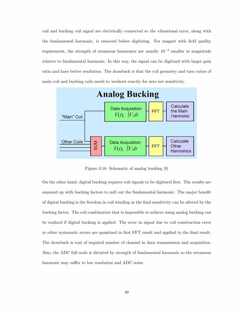
coil and bucking coil signal are electrically connected so the vibrational error, along with
the fundamental harmonic, is removed before digitizing. For magnet with field quality
requirement, the strength of erroneous harmonics are usually 10−4 smaller in magnitude
relative to fundamental harmonic. In this way, the signal can be digitized with larger gain
ratio and have better resolution. The drawback is that the coil geometry and turn ratios of
main coil and bucking coils needs to workout exactly for zero net sensitivity.
Figure 3.18: Schematic of analog bucking [9]
On the other hand, digital bucking requires coil signals to be digitized first. The results are
summed up with bucking factors to null out the fundamental harmonic. The major benefit
of digital bucking is the freedom in coil winding as the final sensitivity can be altered by the
bucking factor. The coil combination that is impossible to achieve using analog bucking can
be realized if digital bucking is applied. The error in signal due to coil construction error
or other systematic errors are quantized in first FFT result and applied to the final result.
The drawback is cost of required number of channel in data transmission and acquisition.
Also, the ADC full scale is dictated by strength of fundamental harmonic so the erroneous
harmonic may suffer to low resolution and ADC noise.
48
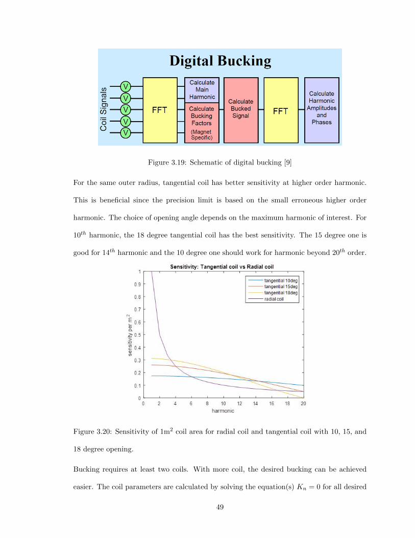
Figure 3.19: Schematic of digital bucking [9]
For the same outer radius, tangential coil has better sensitivity at higher order harmonic.
This is beneficial since the precision limit is based on the small erroneous higher order
harmonic. The choice of opening angle depends on the maximum harmonic of interest. For
10th harmonic, the 18 degree tangential coil has the best sensitivity. The 15 degree one is
good for 14th harmonic and the 10 degree one should work for harmonic beyond 20th order.
Figure 3.20: Sensitivity of 1m2 coil area for radial coil and tangential coil with 10, 15, and
18 degree opening.
Bucking requires at least two coils. With more coil, the desired bucking can be achieved
easier. The coil parameters are calculated by solving the equation(s) Kn = 0 for all desired
49

bucking harmonic n. For example, to buck quadrupole and dipole harmonic for quadrupole
measurement, the following equation has to be solved for all conductors j:
∑j
Njrjeiθj (−1)j = 0
∑j
Njrj2ei2θj (−1)j = 0
RADIAL COIL WITH N=1, N=2 BUCKING
For radial coil, all the conductors lie on x axis. The equations are simplified to:
∑j
Njrj(−1)j = 0
∑j
Njrj2(−1)j = 0
For example, from a radial coil design at DESY, the coil geometry satisfies the equation [17]:
NA (r2 + r1)−NB (r3 + r4)−NC (r5 + r6) = 0
NA
(r2
2 − r12)−NB
(r4
2 − r32)−NC
(r6
2 − r52)
= 0
Figure 3.21: Design of radial coil for quadrupole measurement for HERA collider with
dipole and quadrupole bucking [13].
50
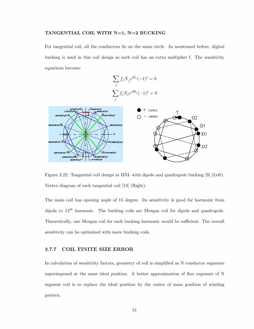
TANGENTIAL COIL WITH N=1, N=2 BUCKING
For tangential coil, all the conductors lie on the same circle. As mentioned before, digital
bucking is used in this coil design so each coil has an extra multiplier f. The sensitivity
equations become: ∑j
fjN jeiθj (−1)j = 0
∑j
fjNjei2θj (−1)j = 0
Figure 3.22: Tangential coil design at BNL with dipole and quadrupole bucking [9] (Left).
Vertex diagram of each tangential coil [13] (Right).
The main coil has opening angle of 15 degree. Its sensitivity is good for harmonic from
dipole to 14th harmonic. The bucking coils are Morgan coil for dipole and quadrupole.
Theoretically, one Morgan coil for each bucking harmonic would be sufficient. The overall
sensitivity can be optimized with more bucking coils.
3.7.7 COIL FINITE SIZE ERROR
In calculation of sensitivity factors, geometry of coil is simplified as N conductor segments
superimposed at the same ideal position. A better approximation of flux exposure of N
segment coil is to replace the ideal position by the center of mass position of winding
pattern.
51
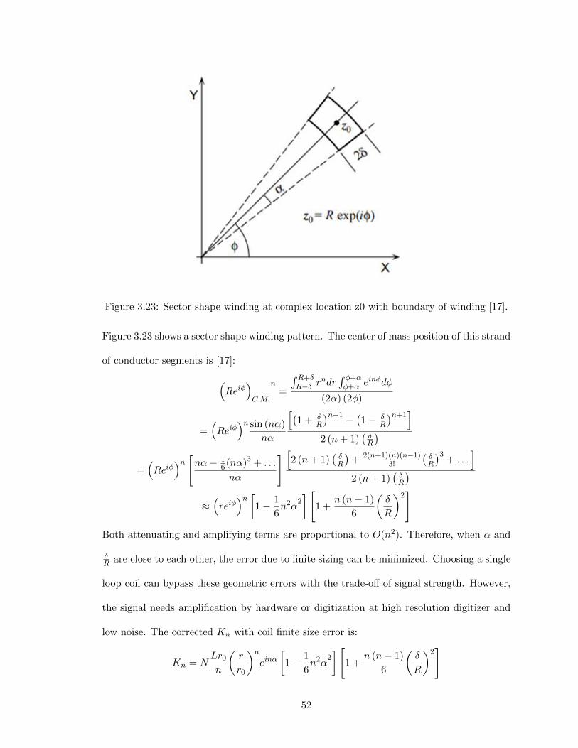
Figure 3.23: Sector shape winding at complex location z0 with boundary of winding [17].
Figure 3.23 shows a sector shape winding pattern. The center of mass position of this strand
of conductor segments is [17]:
(Reiφ
)C.M.
n=
∫ R+δR−δ r
ndr∫ φ+αφ+α e
inφdφ
(2α) (2φ)
=(Reiφ
)n sin (nα)
nα
[(1 + δ
R
)n+1 −(1− δ
R
)n+1]
2 (n+ 1)(δR
)=(Reiφ
)n [nα− 16(nα)3 + . . .
nα
] [2 (n+ 1)
(δR
)+ 2(n+1)(n)(n−1)
3!
(δR
)3+ . . .
]2 (n+ 1)
(δR
)≈(reiφ
)n [1− 1
6n2α
2][
1 +n (n− 1)
6
(δ
R
)2]
Both attenuating and amplifying terms are proportional to O(n2). Therefore, when α and
δR are close to each other, the error due to finite sizing can be minimized. Choosing a single
loop coil can bypass these geometric errors with the trade-off of signal strength. However,
the signal needs amplification by hardware or digitization at high resolution digitizer and
low noise. The corrected Kn with coil finite size error is:
Kn = NLr0
n
(r
r0
)neinα
[1− 1
6n2α
2][
1 +n (n− 1)
6
(δ
R
)2]
52
CHAPTER 4
CONCEPTUAL DESIGN
Argonne National Lab’s rotating wire approach is adapted because of the simplicity. As
mention before, single rotating wire has the simplest and expandable coil geometry. It also
has less vibration during rotation due to negligible sag. As a single conductor coil, it’s
immune to finite size error and winding uncertainty. The low resistance also reduces the
Johnson noise [13].
The drawback is the measurement time since each harmonic has to be measured individually.
The rotation speed needs to be wisely chosen. Calibration work has to take place every time
when wire is disassembled. The hardware requirement is also high. For this approach to
work, the rotation stage pair has to be well aligned and synchronized. A Lock-in amplifier
is necessary to recover the wire signal.
At Radiabeam Technologies, the Newport XPS series motion controller from 3D Hall probe
system has room for two more axes. Also, a Zurich HF2LI Lock-in amplifier is already in
service for the vibrating wire system. Because the Zurich Lock in amplifier provides two
input channels, it makes bucking possible for only one harmonic. To buck two harmonic
simultaneous, the bucking coil needs to be designed properly. Two bucking coils with proper
sensitivity and number of turns will be connected in series. In this thesis, a coil is designed
for the EMQD-280-709 quadrupole magnet characterization but the measurement concept
53

can be generalized to any type of magnet measurement.
Figure 4.1: Flow diagram of rotating wire system with bucking.
Here is the introduction of components in the proposed system:
• Coil: One main coil measures harmonic content and one bucking coil provides bucking
signal for calibration, alignment, and harmonic content measurement.
• Lab computer: Control current in magnet. Control motion of rotary stage via motion
controller. Display and store measurement data from DAQ and Lock-in amplifier.
Conduct a measurement script.
• Power supply: Generate current to excite magnetic field in electromagnet.
• Current sensor: Record current in magnet all the time.
• Motion controller: Control motion of two rotary stages for synchronized motion. Send
out encoder signal to Lock-in Amplifier and DAQ.
• Rotary stage: Drives the rotor part and rotating coil (wire).
• Slip ring: Transmit electrical signal from rotor terminal to static terminal.
• Lock-in amplifier: Read encoder signal and use it as reference signal. Amplify volt-
age signal of individual harmonic from slip ring and perform FFT analysis. Output
amplified voltage signal to DAQ.
54
• DAQ: Measure amplified voltage signal from Lock-in amplifier. Measure time interval
between each rotary encoder count. Perform time integration and FFT analysis.
4.1 COIL
4.1.1 COIL DESIGN AND SENSITIVITY
For good sensitivity in higher order harmonics, tangential design is chosen for both main
and bucking coils. The design is optimized for quadrupole measurement, which means
the harmonic sensitivities other than quadrupole after bucking are maximized. Due to the
channel limit in Lock-in amplifier, the quadrupole bucking coil and dipole bucking coil has to
be connected in series to buck both harmonic simultaneously. An alternative quick solution
would be purchasing one more amplifier channel. The main coil (M) has 15 degree opening
is center at 0 degree position. The quadrupole bucking coil (QB) has 75 degree opening is
center at 180 degree position. The dipole bucking coil (DB) has 180 degree opening angle
at 180 degree position. M coil and QB coil are single turn and have radial size of 24mm.
DB has two turns and the radial size is 13.2mm . Figure 4.2 shows the position and polarity
of vertex for all coils. The length of coil is chosen as 0.5m, which is more than twice of
magnetic length for EMQD-280-709. This should be sufficient to cover the entire fringe
field.
55
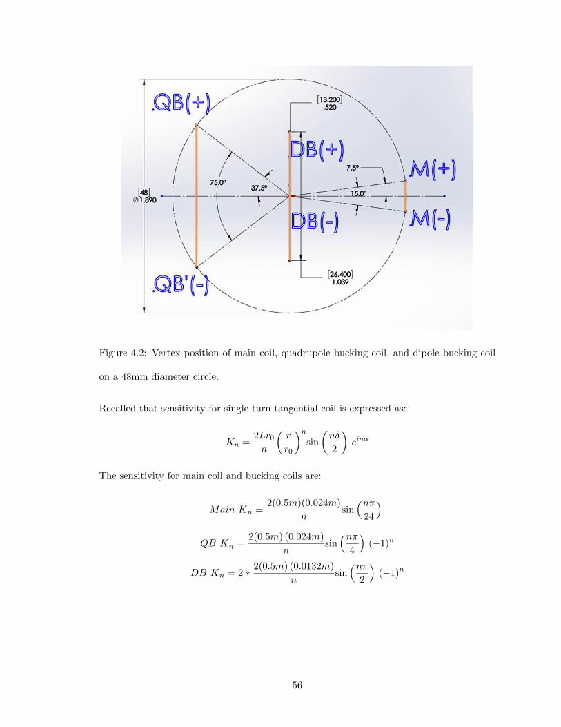
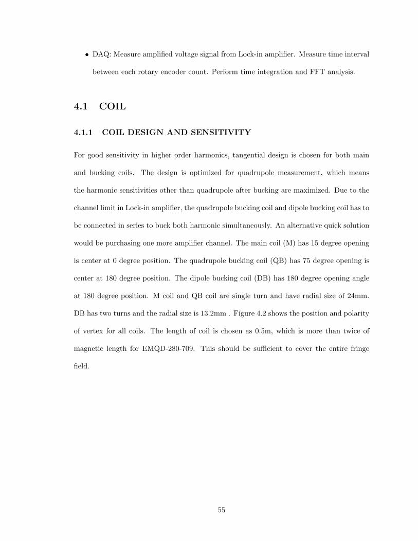
Figure 4.2: Vertex position of main coil, quadrupole bucking coil, and dipole bucking coil
on a 48mm diameter circle.
Recalled that sensitivity for single turn tangential coil is expressed as:
Kn =2Lr0
n
(r
r0
)nsin
(nδ
2
)einα
The sensitivity for main coil and bucking coils are:
Main Kn =2(0.5m)(0.024m)
nsin(nπ
24
)QB Kn =
2(0.5m) (0.024m)
nsin(nπ
4
)(−1)n
DB Kn = 2 ∗ 2(0.5m) (0.0132m)
nsin(nπ
2
)(−1)n
56

Figure 4.3: Sensitivity of main coil.
Figure 4.4: Sensitivity of quadrupole bucking coil for quadrupole magnet measurement.
57
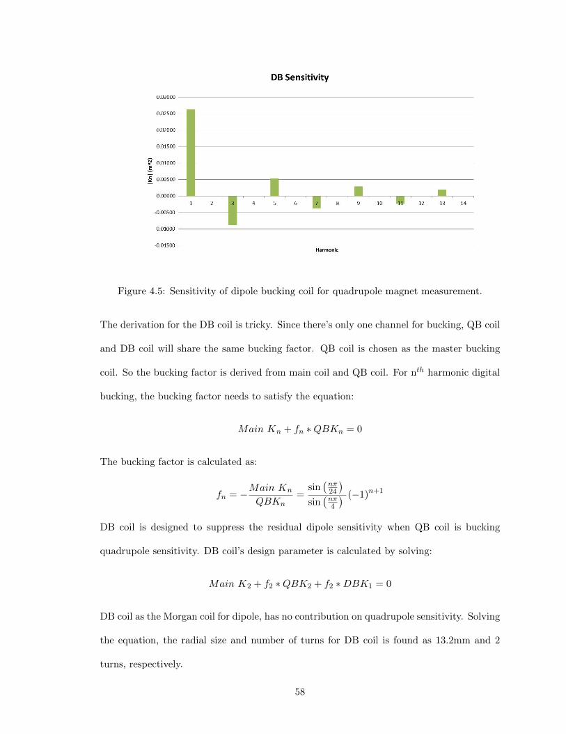
Figure 4.5: Sensitivity of dipole bucking coil for quadrupole magnet measurement.
The derivation for the DB coil is tricky. Since there’s only one channel for bucking, QB coil
and DB coil will share the same bucking factor. QB coil is chosen as the master bucking
coil. So the bucking factor is derived from main coil and QB coil. For nth harmonic digital
bucking, the bucking factor needs to satisfy the equation:
Main Kn + fn ∗QBKn = 0
The bucking factor is calculated as:
fn = −Main Kn
QBKn=
sin(nπ24
)sin(nπ4
) (−1)n+1
DB coil is designed to suppress the residual dipole sensitivity when QB coil is bucking
quadrupole sensitivity. DB coil’s design parameter is calculated by solving:
Main K2 + f2 ∗QBK2 + f2 ∗DBK1 = 0
DB coil as the Morgan coil for dipole, has no contribution on quadrupole sensitivity. Solving
the equation, the radial size and number of turns for DB coil is found as 13.2mm and 2
turns, respectively.
58
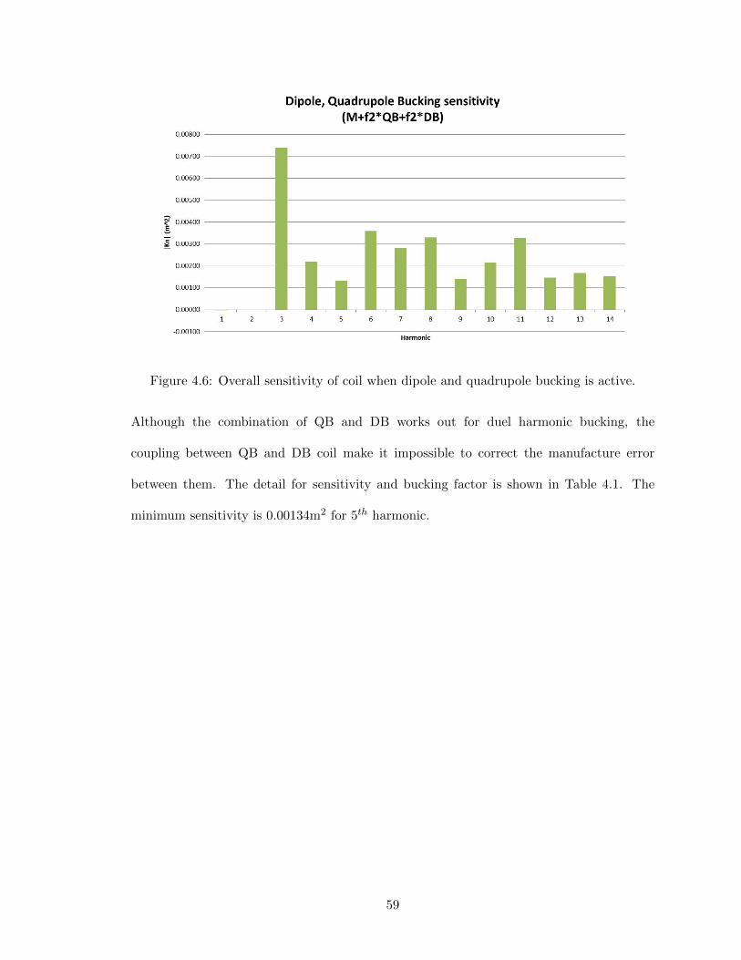
Figure 4.6: Overall sensitivity of coil when dipole and quadrupole bucking is active.
Although the combination of QB and DB works out for duel harmonic bucking, the
coupling between QB and DB coil make it impossible to correct the manufacture error
between them. The detail for sensitivity and bucking factor is shown in Table 4.1. The
minimum sensitivity is 0.00134m2 for 5th harmonic.
59
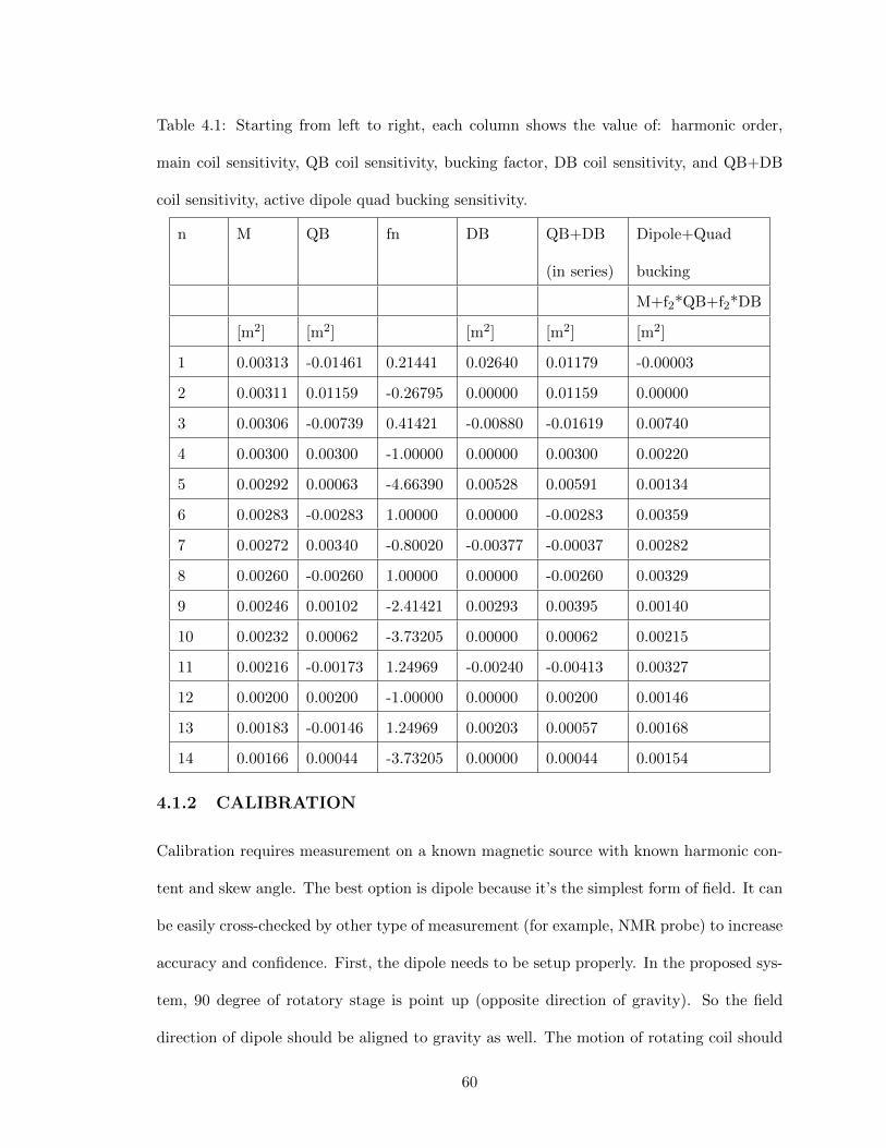
Table 4.1: Starting from left to right, each column shows the value of: harmonic order,
main coil sensitivity, QB coil sensitivity, bucking factor, DB coil sensitivity, and QB+DB
coil sensitivity, active dipole quad bucking sensitivity.
n M QB fn DB QB+DB
(in series)
Dipole+Quad
bucking
M+f2*QB+f2*DB
[m2] [m2] [m2] [m2] [m2]
1 0.00313 -0.01461 0.21441 0.02640 0.01179 -0.00003
2 0.00311 0.01159 -0.26795 0.00000 0.01159 0.00000
3 0.00306 -0.00739 0.41421 -0.00880 -0.01619 0.00740
4 0.00300 0.00300 -1.00000 0.00000 0.00300 0.00220
5 0.00292 0.00063 -4.66390 0.00528 0.00591 0.00134
6 0.00283 -0.00283 1.00000 0.00000 -0.00283 0.00359
7 0.00272 0.00340 -0.80020 -0.00377 -0.00037 0.00282
8 0.00260 -0.00260 1.00000 0.00000 -0.00260 0.00329
9 0.00246 0.00102 -2.41421 0.00293 0.00395 0.00140
10 0.00232 0.00062 -3.73205 0.00000 0.00062 0.00215
11 0.00216 -0.00173 1.24969 -0.00240 -0.00413 0.00327
12 0.00200 0.00200 -1.00000 0.00000 0.00200 0.00146
13 0.00183 -0.00146 1.24969 0.00203 0.00057 0.00168
14 0.00166 0.00044 -3.73205 0.00000 0.00044 0.00154
4.1.2 CALIBRATION
Calibration requires measurement on a known magnetic source with known harmonic con-
tent and skew angle. The best option is dipole because it’s the simplest form of field. It can
be easily cross-checked by other type of measurement (for example, NMR probe) to increase
accuracy and confidence. First, the dipole needs to be setup properly. In the proposed sys-
tem, 90 degree of rotatory stage is point up (opposite direction of gravity). So the field
direction of dipole should be aligned to gravity as well. The motion of rotating coil should
60

be inside of dipole’s good field region all the time. The calibration process measures dipole
field in dipole bucking mode. The result for dipole if often not zero due to error in wire
position. It could indicate a construction error in coil or the non-concentricity between coil
and rotation axis. A new bucking factor F2 can be calculated. Applying the –F2 to bucking
factor can doubles dipole harmonic and gives better calibration accuracy. The calibration
factor is measured as:
Scale factor =|C1|reference|C1|measured
Zero angle = ϕ measured −π
2
The correction needs to be applied on the final harmonic content result.
Figure 4.7: Sensitivity of coil when -f2 is used as bucking factor. Dipole and quadrupole
are amplified to twice.
61
4.1.3 ALIGNMENT
Spill down field error is used to align the magnet. If the axis of rotation is off by distance
∆r, we have
∆Cn−1
(n− 2)!
(∆r
r0
)n−2
=∆Cn
(n− 1)!
(∆r
r0
)n−1
∆Cn−1 =∆Cnn− 1
(∆r
r0
)(4.1)
As the spill-down harmonic of quadrupole, the dipole field is expressed as:
∆C1 = ∆C2
(∆r
r0
)
or
∆B1 = ∆C2
(∆x
r0
)∆A1 = ∆C2
(∆y
r0
)When magnet is aligned to rotation axis, ∆B1 and ∆A1 becomes zero. To conduct this
alignment procedure, the same bucking factor –F2 is used. The dipole harmonic of testing
quadrupole magnet can be measured with twice of sensitivity, which increases the accuracy.
4.1.4 MATERIAL AND POSITIONAL TOLERANCE
The chosen wire is 32 AWG, heavy build wire made by MWS Wire Industry [18]. The OD
of wire is ∼0.01”. Resistance for each coil is less than 1Ohm for 0.5m length. The Johnson
noise for each coils are about 0.01uV at 10 kHz sampling rate. The coil fixture is a simple
rectangular plate made of any easy machines material. If metal is used, insulation will be
required under terminal. The tension-applying feature isn’t added yet. The edge that wire
stays on is rounded to prevent wire breaking.
62
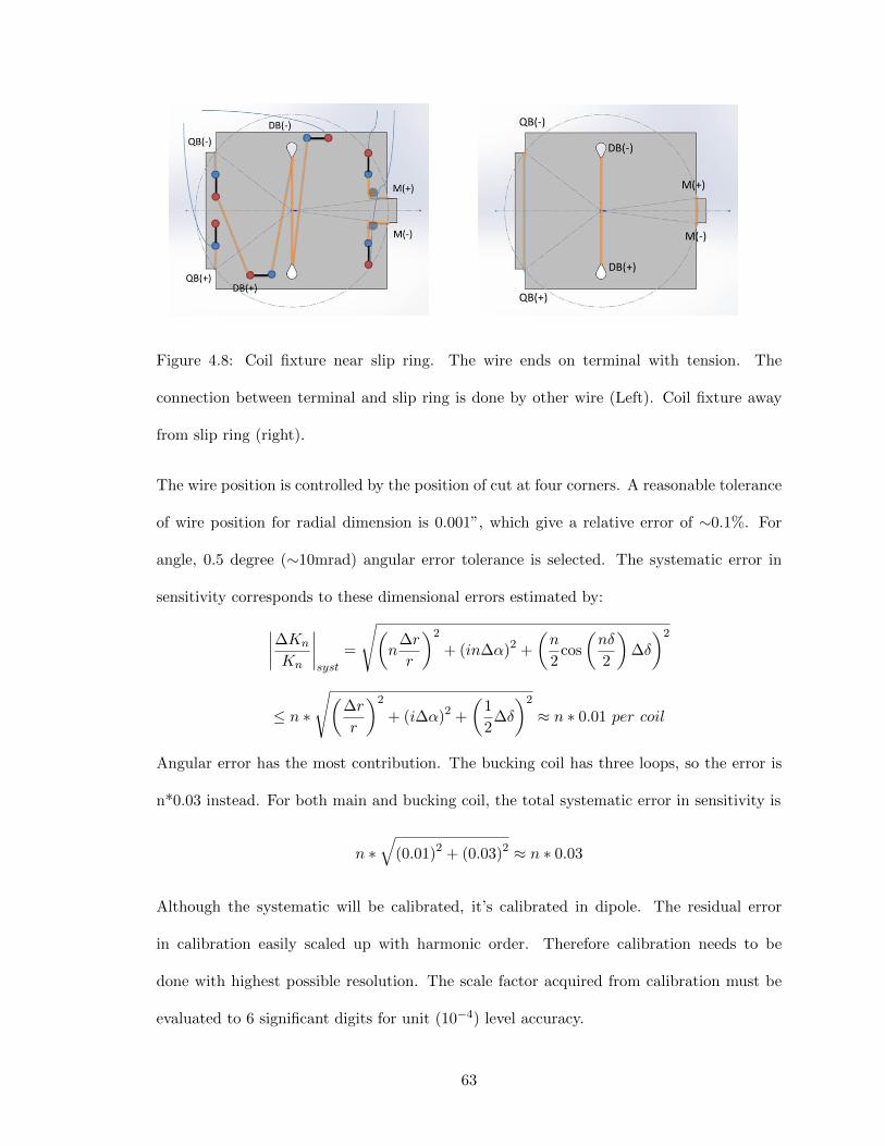
Figure 4.8: Coil fixture near slip ring. The wire ends on terminal with tension. The
connection between terminal and slip ring is done by other wire (Left). Coil fixture away
from slip ring (right).
The wire position is controlled by the position of cut at four corners. A reasonable tolerance
of wire position for radial dimension is 0.001”, which give a relative error of ∼0.1%. For
angle, 0.5 degree (∼10mrad) angular error tolerance is selected. The systematic error in
sensitivity corresponds to these dimensional errors estimated by:
∣∣∣∣∆Kn
Kn
∣∣∣∣syst
=
√(n
∆r
r
)2
+ (in∆α)2 +
(n
2cos
(nδ
2
)∆δ
)2
≤ n ∗
√(∆r
r
)2
+ (i∆α)2 +
(1
2∆δ
)2
≈ n ∗ 0.01 per coil
Angular error has the most contribution. The bucking coil has three loops, so the error is
n*0.03 instead. For both main and bucking coil, the total systematic error in sensitivity is
n ∗√
(0.01)2 + (0.03)2 ≈ n ∗ 0.03
Although the systematic will be calibrated, it’s calibrated in dipole. The residual error
in calibration easily scaled up with harmonic order. Therefore calibration needs to be
done with highest possible resolution. The scale factor acquired from calibration must be
evaluated to 6 significant digits for unit (10−4) level accuracy.
63
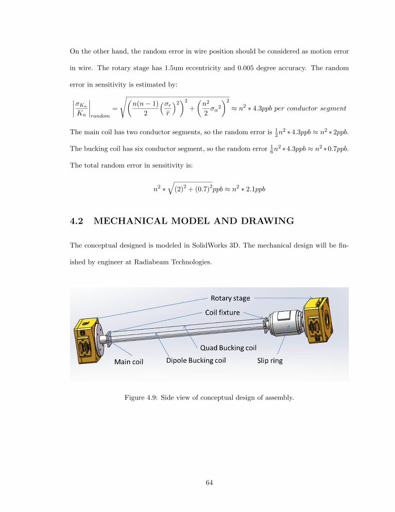
On the other hand, the random error in wire position should be considered as motion error
in wire. The rotary stage has 1.5um eccentricity and 0.005 degree accuracy. The random
error in sensitivity is estimated by:
∣∣∣∣σKnKn
∣∣∣∣random
=
√(n(n− 1)
2
(σrr
)2)2
+
(n2
2σα2
)2
≈ n2 ∗ 4.3ppb per conductor segment
The main coil has two conductor segments, so the random error is 12n
2 ∗ 4.3ppb ≈ n2 ∗ 2ppb.
The bucking coil has six conductor segment, so the random error 16n
2 ∗4.3ppb ≈ n2 ∗0.7ppb.
The total random error in sensitivity is:
n2 ∗√
(2)2 + (0.7)2ppb ≈ n2 ∗ 2.1ppb
4.2 MECHANICAL MODEL AND DRAWING
The conceptual designed is modeled in SolidWorks 3D. The mechanical design will be fin-
ished by engineer at Radiabeam Technologies.
Figure 4.9: Side view of conceptual design of assembly.
64
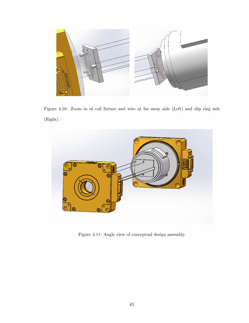
Figure 4.10: Zoom in of coil fixture and wire at far away side (Left) and slip ring side
(Right).
Figure 4.11: Angle view of conceptual design assembly.
65
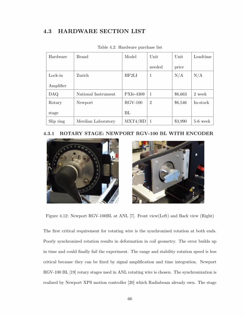
4.3 HARDWARE SECTION LIST
Table 4.2: Hardware purchase list
Hardware Brand Model Unit
needed
Unit
price
Leadtime
Lock-in
Amplifier
Zurich HF2LI 1 N/A N/A
DAQ National Instrument PXIe-4309 1 $6,663 2 week
Rotary
stage
Newport RGV-100
BL
2 $6,546 In-stock
Slip ring Merdian Laboratory MXT4/HD 1 $3,990 5-6 week
4.3.1 ROTARY STAGE: NEWPORT RGV-100 BL WITH ENCODER
Figure 4.12: Newport RGV-100BL at ANL [7]. Front view(Left) and Back view (Right)
The first critical requirement for rotating wire is the synchronized rotation at both ends.
Poorly synchronized rotation results in deformation in coil geometry. The error builds up
in time and could finally fail the experiment. The range and stability rotation speed is less
critical because they can be fixed by signal amplification and time integration. Newport
RGV-100 BL [19] rotary stages used in ANL rotating wire is chosen. The synchronization is
realized by Newport XPS motion controller [20] which Radiabeam already own. The stage
66
has 2 rps maximum rotating speed. Eccentricity is ±1.5um. Rotation speed stability is not
specified but should be decent enough. Maximum encoder resolution is 15000 counts per
revolution. The zero-angle is used as the reference angle for harmonic measurement. The
repeatability of returning to this origin is 0.0001 degree. From the eccentricity 1.5um, the
transverse vibration error can be estimated by:
∆CmC2
=
(K1
Km
)1.5um
24mm=
(K1
Km
)63ppm =
0.00003
0.0013463ppm = 1.4ppm
In worst case scenario, if K1is larger by 0.03 and K5 is smaller by 0.16 due to manufacture
error and calibration didn’t happened, the worst transverse vibration error is 1.7ppm.
In the proposed system, the default rotation speed is picked at 1rps. Only 1000 counts per
revolution will be used in triggering to reduce DAQ time resolution. The sampling rate
for coil signal is set at 10kHz for guarantee triggering. Speed stability needs to be tested
during commission. Assuming the torsion vibration is 0.1 degree. The equivalent error in
harmonic content can be estimated by:
∆CmC2
= 2 ∗(K2
Km
)270ppm
However, the bucking factor is calculated by K2. Therefore the bucking is nearly perfect,
regardless of manufacture error. The torsional vibration error is negligible.
67

4.3.2 ZURICH HF2LI LOCK-IN AMPLIFIER
Figure 4.13: Zurich HF2LI Lock-in amplifier at Radiabeam Technologies.
Lock-in amplifier plays the most important role in rotating wire approach. The signal
collected by single wire is very small (10nV level). When the signal is smaller than con-
ventional amplifier’s internal noise level, the signal is not resolvable regardless of any gain
setting. Lock-in amplifier use phase-sensitive detector that detects signal with typically
x106 narrower bandwidth [21]. The signal is can be recovered to x1000 larger. HF2LI lock-
in amplifier [22] has 120dB dynamic reserve can recover signal that is x10−6 smaller than
its input noise. At 10 kHz sampling rate, the minimum resolvable signal strength would be
2 ∗ 5nV√Hz∗√
10000Hz ∗ 10−6 = 1pV
The input resolution is 14 bit and the minimum scale is 1nV so the resolution is fine
enough to support the 1pV precision. Despite the powerful precision, the resolved signal
is vulnerable to background noise such as electrical noise from stepper motor and slip ring
resistance. These noises will cause systematic error in the FFT result. In measurement,
HF2LI receive encoder signal from motion controller as reference to measure each harmonic,
68
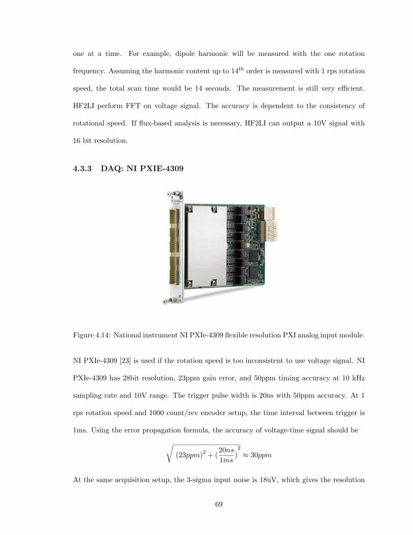
one at a time. For example, dipole harmonic will be measured with the one rotation
frequency. Assuming the harmonic content up to 14th order is measured with 1 rps rotation
speed, the total scan time would be 14 seconds. The measurement is still very efficient.
HF2LI perform FFT on voltage signal. The accuracy is dependent to the consistency of
rotational speed. If flux-based analysis is necessary, HF2LI can output a 10V signal with
16 bit resolution.
4.3.3 DAQ: NI PXIE-4309
Figure 4.14: National instrument NI PXIe-4309 flexible resolution PXI analog input module.
NI PXIe-4309 [23] is used if the rotation speed is too inconsistent to use voltage signal. NI
PXIe-4309 has 28bit resolution, 23ppm gain error, and 50ppm timing accuracy at 10 kHz
sampling rate and 10V range. The trigger pulse width is 20ns with 50ppm accuracy. At 1
rps rotation speed and 1000 count/rev encoder setup, the time interval between trigger is
1ms. Using the error propagation formula, the accuracy of voltage-time signal should be√(23ppm)2 + (
20ns
1ms)2
≈ 30ppm
At the same acquisition setup, the 3-sigma input noise is 18uV, which gives the resolution
69
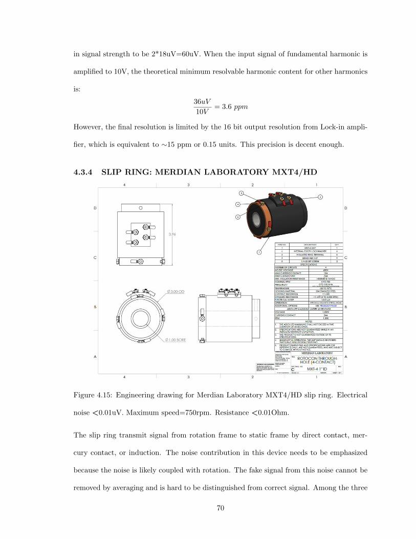
in signal strength to be 2*18uV=60uV. When the input signal of fundamental harmonic is
amplified to 10V, the theoretical minimum resolvable harmonic content for other harmonics
is:
36uV
10V= 3.6 ppm
However, the final resolution is limited by the 16 bit output resolution from Lock-in ampli-
fier, which is equivalent to ∼15 ppm or 0.15 units. This precision is decent enough.
4.3.4 SLIP RING: MERDIAN LABORATORY MXT4/HD
Figure 4.15: Engineering drawing for Merdian Laboratory MXT4/HD slip ring. Electrical
noise <0.01uV. Maximum speed=750rpm. Resistance <0.01Ohm.
The slip ring transmit signal from rotation frame to static frame by direct contact, mer-
cury contact, or induction. The noise contribution in this device needs to be emphasized
because the noise is likely coupled with rotation. The fake signal from this noise cannot be
removed by averaging and is hard to be distinguished from correct signal. Among the three
70

options, the mercury contact way is chosen because of the low noise and low resistance ben-
efits. Merdian Laboratory MXT4/HD has 0.01uV electrical noise and <0.1mOhm contact
resistance. The max speed 750rpm serves our application.
4.4 PROPOSED SYSTEM SPECIFICATION
Parameter of EMQD-280-709 magnet is used to design the coil. The radial size of main coil
and quadrupole bucking coil are the same as the reference radius 24mm. The coil length
is 500mm so all fringe field is covered. The default parameters for operation are the 1
rps rotation speed, 10 kHz sampling rate and, 1000 triggers per revolution. The highest
harmonic to measure is the 14th harmonic. The accuracy and precision are estimated by
systematic error and random error or noise [24]. Repeatability can only be examined based
on real measurement.
4.4.1 ACCURACY
From error propagation section, we know the system accuracy is controlled by the data
acquisition accuracy and systematic error in coil manufacture. The harmonic content and
its relative error due to error from six sources are expressed as:
|Cn| =∣∣∣∣FFT (V s)n
NKn
∣∣∣∣∣∣∣∣∆CnCn
∣∣∣∣ =
√(∆V oltage
Cn
)2
+
(∆time
Cn
)2
+
(∆θ
Cn
)2
+
(∆Kn
Cn
)2
where
∆V oltage
Cn= gain error +
FFT (∆Vsystem noise)n ∗Rotation periodFFT (V s)n
∆time
Cn=
∆ttriggerT/Ns
∆θ
Cn= ein∆θ
71
∣∣∣∣∆Kn
Cn
∣∣∣∣syst
=
√(n
∆r
r
)2
+ (in∆α)2 +
(n
2cos
(nδ
2
)∆δ
)2
In addition, the vibrational error also contributes to systematic error. Although they cannot
be removed calibration, an active bucking measurement can minimize these errors. The
transverse and torsional vibration errors are expressed as:
∆CmCn transverse
= (n− 1)
(Kn−1
Km
)(Dm−n+1
r0
)∆CmCn torsional
= n
(Kn
Km
)Tm−n
The first two terms are calculated in Section 4.3.3. The accuracy of signal acquisition is:√(23ppm)2 + (
20ns
1ms)2
≈ 30ppm
Notice that the system noise error in voltage signal error is not included for now because
it can only be acquired by background measurement during commission. The third term
can be removed by performing measurement in both rotation directions. The forth term is
calculated in Section 4.1.4. The accuracy limit due to manufacture error in coil is:
n ∗ 0.03
where n is the order of harmonic. The fifth and sixth terms are discussed in section 4.3.1.
The effect of transverse vibration due rotary stage’s eccentricity is estimated as 1.4ppm in
worst case scenario (n=5). The effect of torsional vibration is zero due to digital bucking
treatment.
The known overall system accuracy is:
√(30ppm)2 + (n ∗ 0.03)2 + (1.4ppm)2 ≈ n ∗ 0.03
It’s clear that the coil manufacture error controls the overall error in harmonic content
accuracy. When calibration is properly done, the accuracy of system should be reduced to
72

∼30ppm plus the accuracy of calibration source. At Radiabeam, the most accurate magnetic
field sensor is SENIS F3A Hall probe [25], which has 0.1% accuracy. The calibrated accuracy
of system would be: √(30ppm)2 + 0.1%2 ≈ 0.1%
The accuracy can be improved with better reference measurement device. Typical NMR
probe with ppm level accuracy can greatly improve the accuracy to 30ppm. There are
unknown sources of systematic error that need to be evaluated during commission.
4.4.2 PRECISION
We know the harmonic content is calculated by the voltage or flux signal being measured
and the coil sensitivity. The precision of |Cn| cannot be better than precision of FFT (V s)n
and precision of Kn.
|Cn| =∣∣∣∣FFT (V s)n
NKn
∣∣∣∣∣∣∣∣σCnCn∣∣∣∣ =
√(σV oltageCn
)2
+
(σtimeCn
)2
+
(σKnCn
)2
At 10 kHz, the minimum resolvable signal by Lock-in amplifier is 1pV. This precision is
high that it will not be the limiting factor of this system. From section 4.3.3, we know the
minimum resolvable harmonic content in voltage signal is 15ppm. Assuming the random
error in integration time the same as its accuracy, the second term is:
20ns
1ms= 20ppm
The last term is calculated in section 4.1.4. The random error in Kn is calculated as: n2 ∗
2.1ppb. For 14th harmonic (worst case), the random error is 0.4ppm. The known overall
precision of this system is:
√(15ppm)2 + (20ppm)2 + (0.4ppm)2 ≈ 25ppm
73

It means that when the fundamental harmonic is measured and presented as 10000 units, the
other harmonics are precise to 0.25units. The first and second term cannot be reduced by
number of measurement because they are the minimum resolution of this system. Therefore
the minimum resolution of this system is 25ppm.
4.5 MEASUREMENT PROCEDURE
The example measurement procedure for quadrupole is:
1. Preparation
1.1. Setup target magnet on a kinematic stand at middle of test bench
1.2. Initialize rotary stage, verified synchronization, return to origin
1.3. Install coil fixture on rotation stage
1.4. Rough align and center the magnet with respect to rotations axis using laser
1.5. Put wire on coil fixture to create main coil, dipole bucking coil, and quadrupole bucking
coil
1.6. Apply tension on each coil
2. Calibration
2.1. Setup calibration dipole around coil
2.2. Level dipole to gravity
2.3. Turn on calibration field
2.4. Connect coil terminal and slip ring terminal.
2.5. Start rotation
2.6. Measures dipole strength by M coil and QB coil
2.7. Calculate bucking factor F2
2.8. Apply -F2 bucking factor and measure dipole strength C1
2.9. Calculate scaling factor and zero-angle
74

2.10. Turn off calibration field and put away dipole magnet
3. Alignment
3.1. Turn on target magnet to nominal value
3.2. Apply -F2 bucking factor and measure dipole strength C1
3.3. Adjust magnet position to minimized dipole reading
3.4. Record the residual dipole field
4. Fundamental harmonic measurement
4.1. Apply -F2 bucking factor and measure quadrupole strength C2
5. Harmonic content measurement
5.1. Apply F2 bucking factor and measure nth harmonic strength Cn
5.2. Measure nth harmonic strength Cn with main coil (for comparison)
6. Repeat step 4 and 5 for different condition (Transfer function, remnant field measure-
ment, center shift measurement)
7. Reverse rotation direction to remove minimum angle step error
8. Save measurement data
9. Correct raw data with scaling factor and zero-angle
9. Turn off motion
10. Turn off target magnet
11. Disconnect coil
12. Remove target magnet The motion control, power supply control and measurement
control are done in LabView interface. The measurement in step 4 and 5 are actually done
at the same time.
75
CHAPTER 5
SUMMARY
Quality assurance in accelerator magnet is important to ensure functionality of accelerator
system and quality of experiment data. The quality of magnet is determined by the har-
monic content. The harmonic content can be measured by induction, Lorentz force, and
Hall effect. Among all the approaches, the rotating coil method based on induction is the
most practical and efficient one. A real measurement on EMQD-280-709, a diamond shape
quadrupole magnet, is performed based on 3D hall probe method. This single scan mea-
surement takes roughly 4 hours to collect raw data that’s resolvable up to only 6th order
harmonic. The alignment is not included. Using rotating coil method, the measurement
would finish within 30 minute with higher resolvable harmonics and more than ten times of
redundant scans.
The theory of rotating coil method is thoroughly discussed in Chapter 3. The derivation
starts with multipole expansion of magnetic field in cylindrical coordinate. Using the prop-
erty of the periodicity in each harmonic, a harmonic decomposition method is introduced
to calculate harmonic content from given field map. The field quality is then determined.
The second part of chapter 3 introduces four different types of rotating coil design and the
sensitivity of each design. Due to induction, the flux variance sensed by coil is measured
as voltage signal. The sinusoidal signal is then by analyzed by Fourier transformation to
76
come up with harmonic content. Time integration process is added to correct the effect of
inconsistent rotation speed.
In the last section of chapter 3, error propagation is derived for error in signal strength,
timer, angular position, and coil geometry. The effect of transverse and torsional vibration
is also discussed. Because systematic error cause by vibration cannot be removed by cali-
bration, the treatment by bucking is introduced. The bucking method requires additional
coils to generate counter signal to cancel the error due to vibration. The bucking coils can
be directly connected to main coil (analog bucking) or digitized by individual digitizer (dig-
ital bucking). The digital bucking approach allows re-scaling for signal strength. Therefore,
coils can be designed with more freedom.
Based on technology survey in chapter 2 and current apparatus, the rotating wire approach
in Argonne National Laboratory is adopted. The best feature of this approach is the
simplicity in coil winding and flexibility in coil length and radial size. The challenges in
this approach are the extremely low signal strength and shaft-free rotation mechanism.
The first difficulty can be solved by lock-in amplifier, which typical resolves input signal
at nV level by noise reduction. The second difficulty can be solved by twin rotary stage
in synchronization. On top of the existed design, bucking coil is added to enable bucking
capability for two harmonics simultaneously.
In chapter 4, the conceptual system of rotating wire is built. A set of coils is designed
for the example quadrupole magnet. Since our lock-in amplifier model (HF2LI by Zurich
Instruments) has only two input channels, the bucking coil needs to provide bucking for
dipole and quadrupole harmonic simultaneously. A winding design is worked out and pro-
vides full bucking in quadrupole and 30ppm bucking for dipole harmonic. In operation,
the two rotary stages (RGV 100BL by Newport Corporation) rotates at 1 rps speed. The
motion controller is set to outputs encoder signal of 1000 counts per revolution to trigger
77
measurement in lock-in amplifier and DAQ (NI-PXIe-4309). The induced voltage signal
from coil is amplified by HF2LI and output to DAQ (NI-PXIe-4309) for time integration.
Both lock-in amplifier and DAQ are sampling at 10 kHz. After fast Fourier transforma-
tion, the harmonic content up to 14th order is recorded and presented in real time. The
hardware specification, coil manufacture error, and operating parameter are used in error
propagation. After calibration, the accuracy and precision of this proposed system are 0.1%
and 25ppm, respectively. The accuracy is limited by the available reference measurement
at Radiabeam in calibration process. If a NMR probe (typical accuracy is at ppm level) is
used instead, the accuracy of proposed system can be improved to 30ppm at most. Lastly, a
procedure of quadrupole measurement is introduced. Each measurement requires prepara-
tion, calibration, alignment, and field content scan. Estimated time for single field content
scan takes 15 seconds.
78

BIBLIOGRAPHY
[1] Marco Buzio. ”Overview of Magnetic Measurements for Particle Accelerators”. Inter-
national Magnetic Measurement Workshop 20, 2017.
[2] L. Walckiers. ”Magnetic measurements with coils and wires”. 2011.
[3] A. Jain and R. Thomas. ”Fiducialization and Calibration of Rotating Coil for Mag-
netic Measurement of the ERL Quadrupoles”. Technical report, Brookhaven National
Laboratory Magnet Division Note 646-11 (AM-MD-346), 2006.
[4] E. De Matteis, P. Arpaia, and S. Russenschuck. ”Magnetic field mapper based on
rotating coil”. PhD thesis, University degli Studi del Sannio and CERN, 2016.
[5] P. Arpaia, M. Buzio, R. De Oliveria, J. DiMarco, and G. Severino. ”A high-precision
miniaturized rotating coil transducer for magnetic measurements”. Sensor and Actu-
ators A: Physical, 2018.
[6] C. Doose. ”Performance of rotating wire magnetic alignment system for the Advanced
Photon Source Upgrade”. International Magnetic Measurement Workshop 20, 2018.
[7] C. Doose and M.Kasa. ”Multipole magnetic measurement using a lock-in Amplifier
Technique”. North American Particle Accelerator Conference 2013, 2013.
[8] Stephane Sanfilippo. ”Challenges for the magnetic projects at the Paul Scherrer Insti-
tut”. International Magnetic Measurement Workshop 20, 2018.
79
[9] Animesh Jain. ”Harmonic Coils. US particle accelerator school, Santa Babara, CA,
2003.
[10] Animesh Jain. ”Rotating Coil Measurement Errors*”. 2nd Workshop on Beam Dy-
namics Meets Magnets (BeMa2014), 2014.
[11] Jack T. Tanabe. ”Iron Dominated Electromagnets”. ”World Scientific”, 2005.
[12] Animesh Jain. ”Magneti Design for Low Emittance Storage Rings”. MEDSI 2014,
2014.
[13] J. Dimarco. ”Fundamentals of Magnetic Measurement with Rotating Coils: A Tuto-
rial”. International Magnetic Measurement Workshop 19, 2015.
[14] B.C Brown, P.O. Mazur, J.F Ostiguy, S.M. Pruss, and F. Turkot. ”Harmonic Analysis
of Fermilab Main Ring Quadrupoles”. Fermilab-Conf-91/128, 1991.
[15] F. Nicosia and J. Dimarco. ”Magnetic field measurement system based on rotating
PCB coils”. 2014.
[16] Lloyd N. Trefethen and J.A.C Weideman. ”The Exponentially Convergent Trapezoidal
Rule”. SIAM Review, 2014.
[17] Animesh Jain. ”Harmonic Coils”. CERN Report 98-05, pp. 143-173, 1997.
[18] MWS Wire Industries. ”MWS Wire Industries Copper Magnet Wire Data”. https:
//mwswire.com/magnet-wire/round-copper-magnet-wire/ Accessed: 2018-11-27.
[19] Newport Corporation. ”RGV100BL-S Data Sheet”. https://www.newport.com/mam/
celum/celum_assets/resources/RGV100BL-S_Data_Sheet.pdf?1 Accessed: 2018-
11-27.
80
[20] Newport Corporation. ”Trigger Synchronization using a New-
port XPS Series Motion Controller”. https://www.newport.
com/medias/sys_master/images/images/hc9/h76/8797213327390/
Motion-Tech-Note-Trigger-Synchronization-with-XPS-Controller.pdf Ac-
cessed: 2018-11-27.
[21] Stanford Research System. ”About Lock-In Amplifier”.
[22] Zurich Instruments. ”HF2LI 50MHz Lock-in Amplifier”. https://www.zhinst.com/
sites/default/files/zi_hf2li_leaflet_web_0.pdf Accessed: 2018-11-27.
[23] National Instruments. ”NI PXIe 4309”. http://www.ni.com/pdf/manuals/377030a.
pdf Accessed: 2018-11-27.
[24] L. Walckiers, L. Bottura, M. Buzio, P. Schnizer, and N. Smirnov. ”Sensitivity and
Accuracy of the System for the Magnetic Measurement of the LHC Magnets at CERN”.
Proceedings of EPAC 2000, Vienna, Austria, 2000.
[25] SENIS Magnetic & current measurement. ”F3A Magnetic Field Trans-
ducers”. http://c1940652.r52.cf0.rackcdn.com/5791e6b4ff2a7c38fb000a95/
f3a-magnetic-transducer-datasheet_rev03.pdf Accessed: 2018-11-27.
81
Yung-Chuan ChenEducation
University of California, Los Angeles
B.S,, Physics, 2011.
Minor in Mathematics
Indiana University, Bloomington
M.S,, Beam Physics and Technology, 2019.
Experience
2011-present Radiabeam Technologies Santa Monica, CA
Magnet Engineer
Magnet design, simulation, and engineering
Magnet measurement and fiducializtion
Metrology system maintenance and upgrade
Fabrication inspection
82