concepts of database management eighth...

Concepts of Database Management

Eighth Edition

Chapter 2

The Relational Model 1: Introduction, QBE, and Relational Algebra

Relational Databases

• A relational database is a collection of tables

• Each entity is stored in its own table

• Attributes of an entity become the fields or columns

in the table

• Relationships are implemented through common

columns in two or more tables

• Should not permit multiple entries (repeating

groups) in a table

2

Relational Databases (continued)

• Relation: two-dimensional table in which:

– Entries are single-valued

– Each column has a distinct name (called the

attribute name)

– All values in a column are values of the same

attribute

– Order of columns is immaterial

– Each row is distinct

– Order of rows is immaterial

3


• Relational database: collection of relations

• Unnormalized relation

– A structure that satisfies all properties of a relation

except for the first item

– Entries contain repeating groups; they are not

single-valued

4


• Database structure representation

– Write name of the table followed by a list of all

columns within parentheses

– Each table should appear on its own line

– Notation to be used with duplicate column names

within a database: Tablename.Columnname

• You qualify the column names

• Primary key: column or collection of columns of a

table (relation) that uniquely identifies a given row

in that table

5

Query-by-Example (QBE)

• Query: question represented in a way the DBMS

can recognize and process

• Query-By-Example (QBE)

– Visual approach to writing queries

– Users ask their questions using an on-screen grid

– Data appears on the screen in tabular form

6

Query-by-Example (QBE) (continued)

• Query window in Access has two panes

– Upper portion contains a field list for each table you

want to query

– Lower pane contains the design grid, where you

specify:

• Format of output

• Fields to be included in the query results

• Sort order for query results

• Any criteria the records must satisfy

7

Simple Queries

• To include a field in an Access query, double-click

the field in the field list to place it in the design grid

• Clicking Run button in Results group on the

QUERY TOOLS DESIGN tab runs query and

displays query results

• Add all fields from a table to the design grid by

double-clicking the asterisk in the table’s field list

8

Simple Queries (continued)

9

FIGURE 2-3: Fields added to the design grid

Simple Queries (continued)

FIGURE 2-4: Query results

10

Simple Criteria

• Criteria: conditions that data must satisfy

• Criterion: single condition that data must satisfy

• To enter a criterion for a field:

– Include field in the design grid

– Enter criterion in Criteria row for that field

11

Simple Criteria (continued)

• Comparison operator

– Also called a relational operator

– Used to find something other than an exact match

= (equal to)

> (greater than)

< (less than)

>= (greater than or equal to)

<= (less than or equal to)

NOT (not equal to)

12

Compound Criteria

• Compound criteria, or compound conditions

– AND criterion: both criteria must be true for the

compound criterion to be true

– OR criterion: either criteria must be true for the

compound criterion to be true

• To create an AND criterion in QBE:

– Place the criteria for multiple fields on the same

Criteria row in the design grid

• To create an OR criterion in QBE:

– Place the criteria for multiple fields on different

Criteria rows in the design grid

13

Compound Criteria (continued)

FIGURE 2-9: Query that uses an AND criterion

14

Compound Criteria (continued)

FIGURE 2-11: Query that uses an OR criterion

15

Computed Fields

• Computed field or calculated field

– Result of a calculation on one or more existing fields

• To include a computed field in a query:

– Enter a name for the computed field, followed by a

colon, followed by an expression in one of the

columns in the Field row

• Alternative method

– Right-click the column in the Field row, and then

click Zoom to open the Zoom dialog box

– Type the expression in the Zoom dialog box

16

Computed Fields (continued)

FIGURE 2-15: Query that uses a computed field

17

Functions

• Count

• Sum

• Avg (average)

• Max (largest value)

• Min (smallest value)

• StDev (standard

deviation)

• Var (variance)

• First

• Last

• Built-in functions

– Called aggregate functions in Access

18

Functions (continued)

FIGURE 2-17: Query to count records

19

Functions (continued)

FIGURE 2-18: Query results

20

Grouping

• Grouping: creating groups of records that share

some common characteristic

• To group records in Access:

– Select Group By operator in the Total row for the

field on which to group

21

Grouping (continued)

FIGURE 2-21: Query to group records

22

Sorting

• Sorting: listing records in query results in an

ordered way

• Sort key: field on which records are sorted

• Major sort key

– Also called the primary sort key

– First sort field, when sorting records by more than

one field

• Minor sort key

– Also called the secondary sort key

– Second sort field, when sorting records by more than

one field

23

Sorting (continued)

FIGURE 2-23: Query to sort records

24

Sorting on Multiple Keys

• Specifying more than one sort key in a query

• Major (primary) sort key

– Sort key on the left in the design grid

• Minor (secondary) sort key

– Sort key on the right in the design grid

25

Sorting on Multiple Keys (continued)

FIGURE 2-27: Correct query design to sort by RepNum and then by

CustomerName

26

Joining Tables

• Queries to select data from more than one table

• Join the tables based on matching fields in

corresponding columns

• Join line

– Line drawn by Access between matching fields in

the two tables

– Indicates that the tables are related

27

Joining Tables (continued)

FIGURE 2-29: Query design to join two tables

28

Joining Multiple Tables

• Joining three or more tables is similar to joining two

tables

• To join three or more tables:

– Add the field lists for all tables in the join to upper

pane

– Add the fields to appear in query results to design

grid in the desired order

29

Using an Update Query

• Update query: a query that changes data

– Makes a specified change to all records satisfying

the criteria in the query

• To change a query to an update query:

– Click Update button in the Query Type group on the

QUERY TOOLS DESIGN tab

• Update To row is added when an update query is

created

– Used to indicate how to update data selected by the

query

30

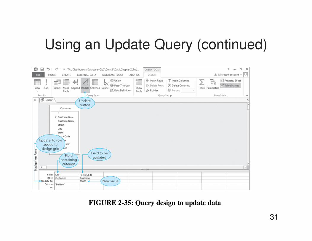
Using an Update Query (continued)

FIGURE 2-35: Query design to update data

31

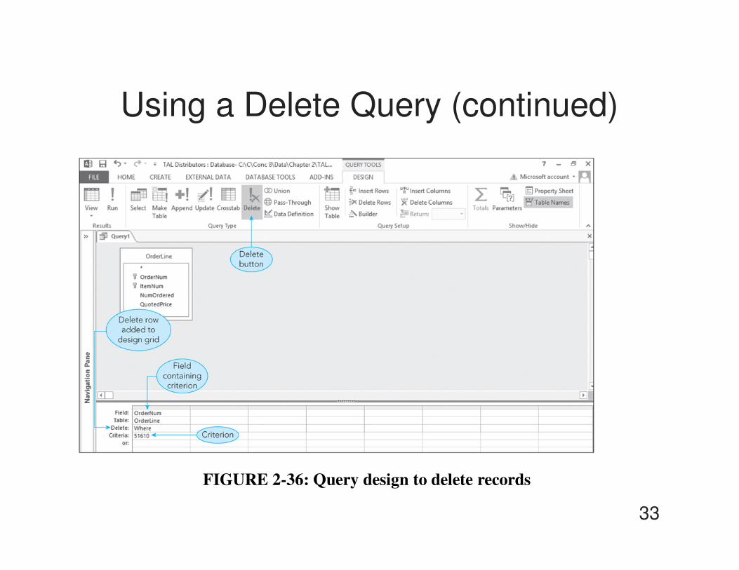
Using a Delete Query

• Delete query: permanently deletes all records

satisfying the criteria entered in the query

• To change query type to a delete query:

– Click Delete button in the Query Type group on the

QUERY TOOLS DESIGN tab

• Delete row is added

– Indicates this is a delete query

32

Using a Delete Query (continued)

FIGURE 2-36: Query design to delete records

33

Using a Make-Table Query

• Make-table query: creates a new table using

results of a query

• Records added to new table are separate from the

original table

• To change the query type to a make-table query:

– Click Make Table button in the Query Type group on

the QUERY TOOLS DESIGN tab

– In Make Table dialog box, enter the new table’s

name and choose where to create it

34

Using a Make-Table Query (continued)

FIGURE 2-38: Make Table dialog box

35

Relational Algebra

• Theoretical way of manipulating a relational

database

• Includes operations that act on existing tables to

produce new tables

• Each command ends with a GIVING clause,

followed by a table name

– Clause requests the result of the command to be

placed in a temporary table with the specified name

36

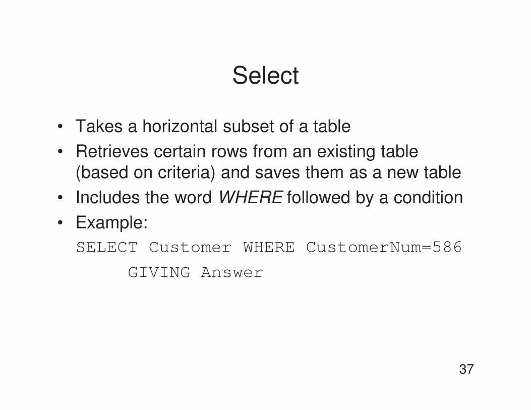
Select

• Takes a horizontal subset of a table

• Retrieves certain rows from an existing table

(based on criteria) and saves them as a new table

• Includes the word WHERE followed by a condition

• Example:

SELECT Customer WHERE CustomerNum=586

GIVING Answer

37

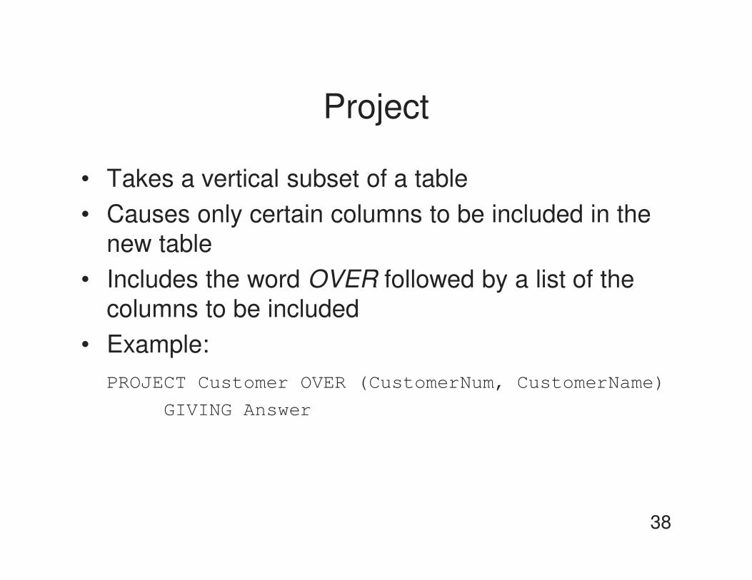
Project

• Takes a vertical subset of a table

• Causes only certain columns to be included in the

new table

• Includes the word OVER followed by a list of the

columns to be included

• Example:

PROJECT Customer OVER (CustomerNum, CustomerName)

GIVING Answer

38

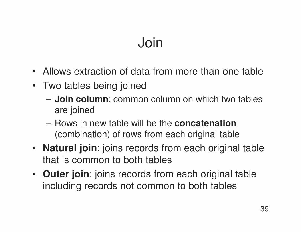
Join

• Allows extraction of data from more than one table

• Two tables being joined

– Join column: common column on which two tables

are joined

– Rows in new table will be the concatenation(combination) of rows from each original table

• Natural join: joins records from each original table

that is common to both tables

• Outer join: joins records from each original table

including records not common to both tables

39

Normal Set Operations

• Union of tables A and B

– Table containing all rows that are in either table A or

table B or in both table A and table B

• Intersection of tables A and B

– Table containing all rows that are common in both

table A and table B

• Difference of tables A and B

– Referred to as A minus B

– Set of all rows that are in table A but that are not in

table B

40

Union

• Two tables are union compatible when:

– They have the same number of columns

– Corresponding columns represent the same type of

dataJOIN Orders, Customer

WHERE Orders.CustomerNum=Customer.CustomerNum

GIVING Temp1

PROJECT Temp1 OVER CustomerNum, CustomerName

GIVING Temp2

SELECT Customer WHERE RepNum=‘30'

GIVING Temp3


GIVING Temp4

UNION Temp2 WITH Temp4 GIVING Answer

41

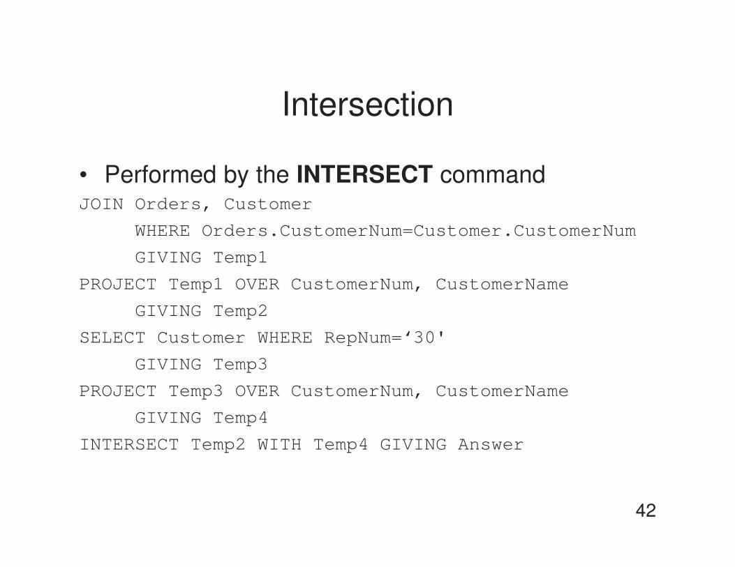
Intersection

• Performed by the INTERSECT commandJOIN Orders, Customer


GIVING Temp1


GIVING Temp2


GIVING Temp3


GIVING Temp4

INTERSECT Temp2 WITH Temp4 GIVING Answer

42

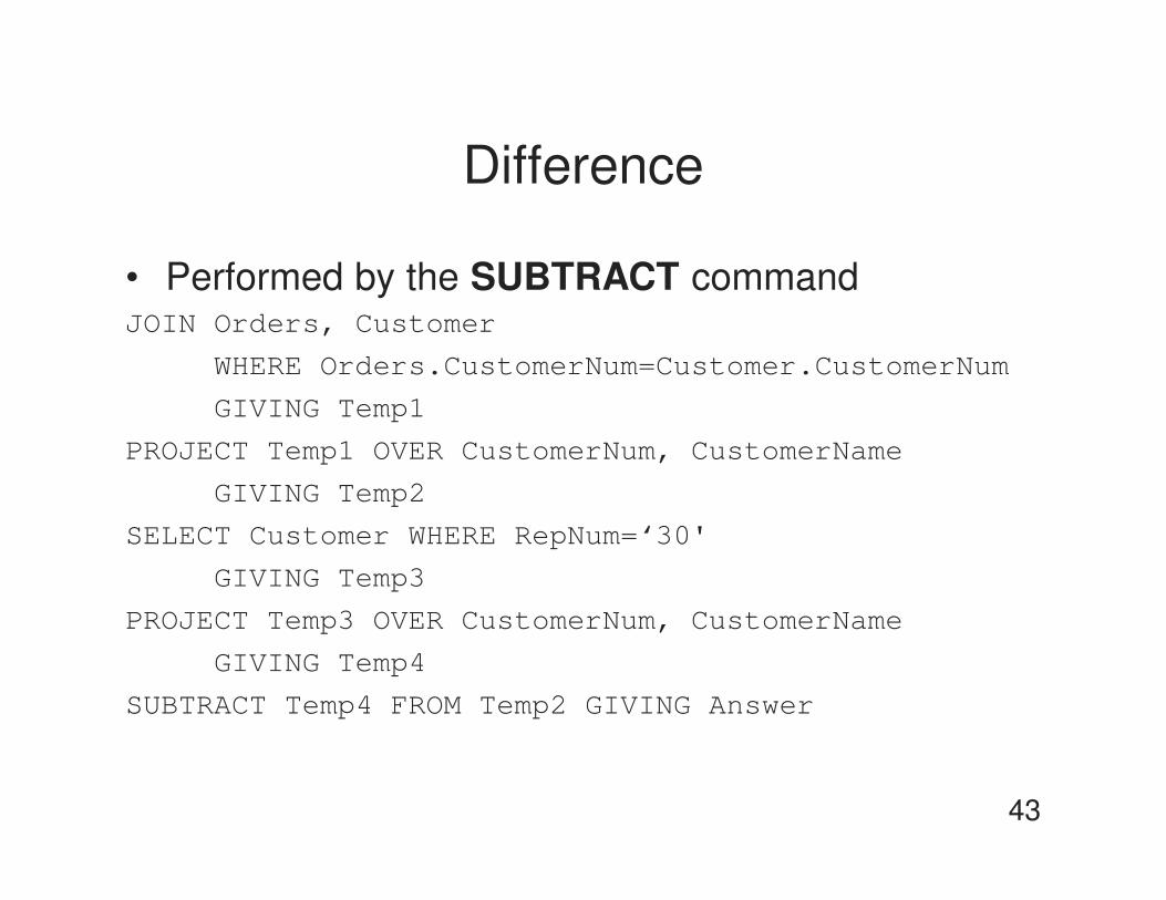
Difference

• Performed by the SUBTRACT commandJOIN Orders, Customer


GIVING Temp1


GIVING Temp2


GIVING Temp3


GIVING Temp4

SUBTRACT Temp4 FROM Temp2 GIVING Answer

43

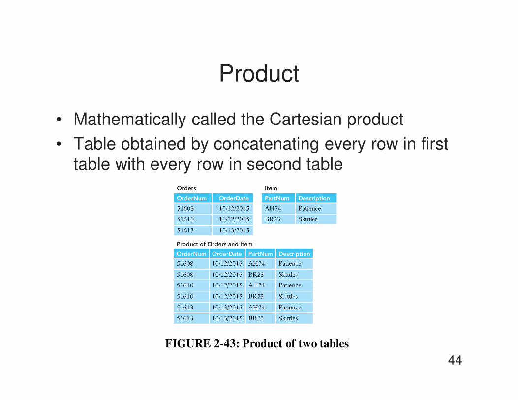
Product

• Mathematically called the Cartesian product

• Table obtained by concatenating every row in first

table with every row in second table

FIGURE 2-43: Product of two tables

44

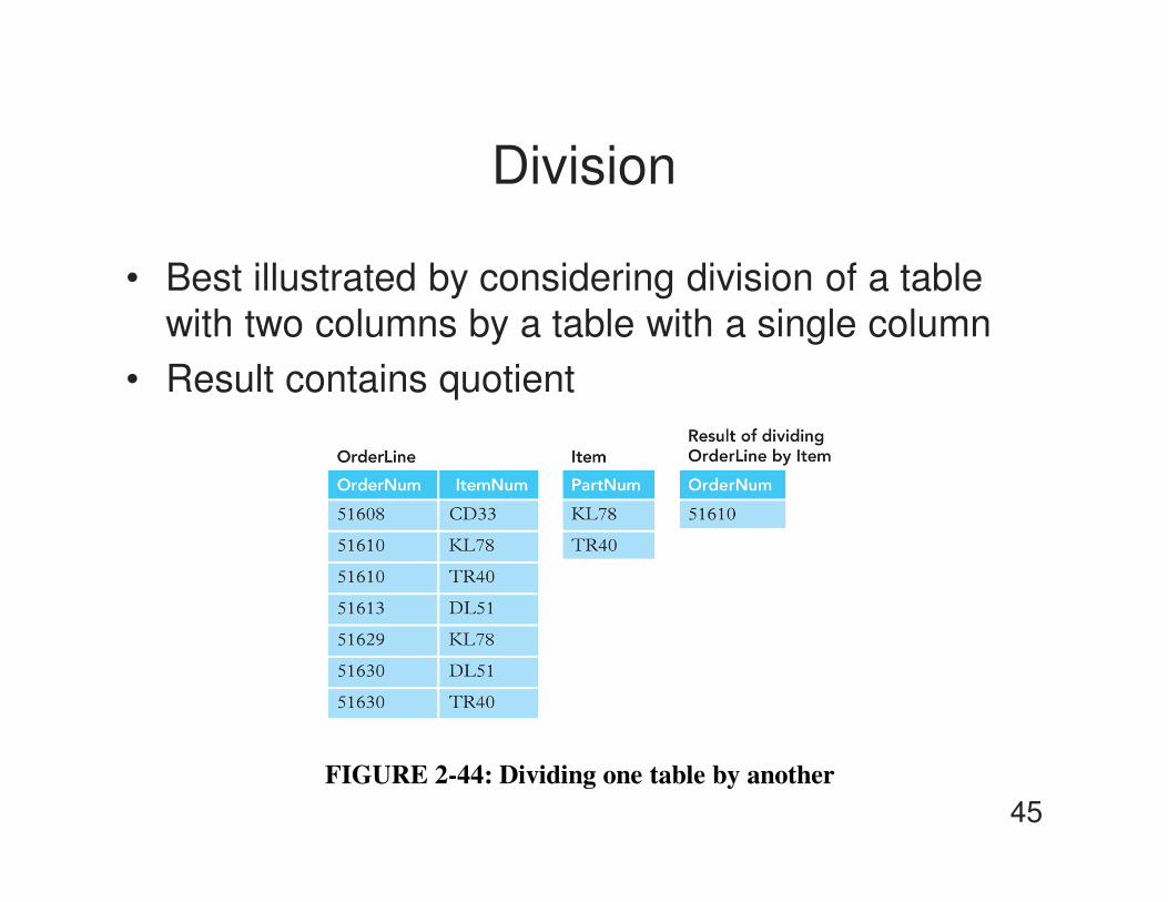
Division

• Best illustrated by considering division of a table

with two columns by a table with a single column

• Result contains quotient

FIGURE 2-44: Dividing one table by another

45

concepts of database management eighth...

Documents