Psychological Methods2001, Vol. 6, No. 4,430-^50

Copyright 2001 by the American Psychological Association, Inc.1082-989X/01/S5.00 DOI: 10.1037//1082-989X.6.4.430

Computing and Evaluating Factor Scores

James W. GriceOklahoma State University

A variety of methods for computing factor scores can be found in the psychologicalliterature. These methods grew out of a historic debate regarding the indeterminatenature of the common factor model. Unfortunately, most researchers are unawareof the indeterminacy issue and the problems associated with a number of the factorscoring procedures. This article reviews the history and nature of factor scoreindeterminacy. Novel computer programs for assessing the degree of indeterminacyin a given analysis, as well as for computing and evaluating different types of factorscores, are then presented and demonstrated using data from the Wechsler Intelli-gence Scale for Children—Third Edition. It is argued that factor score indetermi-nacy should be routinely assessed and reported as part of any exploratory factoranalysis and that factor scores should be thoroughly evaluated before they arereported or used in subsequent statistical analyses.

Exploratory factor analysis is a widely used multi-variate statistical procedure in psychological research.Undoubtedly one of its appeals is the ability to com-pute scores for the individuals in the analysis on theextracted factors. These novel factor scores can beused in a wide variety of subsequent statistical analy-ses. For instance, they can be correlated with mea-sures of different constructs to help clarify the natureof the factors or they can be entered as predictor vari-ables in multiple regression analyses or as dependentvariables in analyses of variance. Factor scores arealso routinely computed as simple sum scores in thescale development process and are often referred to asscale, composite, or total scores. Given these varieduses, it is not surprising that factor scores are commonin the psychological literature.

Computing factor scores is not a straightforwardprocess, however, as researchers must choose from anumber of competing computational methods. For ex-

Development of this article was supported by a summerresearch fellowship awarded to James W. Grice from South-ern Illinois University at Edwardsville. I thank Richard J.Harris at the University of New Mexico for his commentson an earlier draft of this article. Naturally, any errors thatremain are my own.

Correspondence concerning this article should be ad-dressed to James W. Grice, Psychology Department, 215North Murray, Oklahoma State University, Stillwater, Okla-homa 74078. Electronic mail may be sent to jgrice®okstate.edu.

ample, consider three researchers who conduct an ex-ploratory common factor analysis on a questionnaire.Each decides on the same number of factors; uses thesame extraction, rotation, and interpretation proce-dures; and then decides to compute scores for theidentified factors. The first researcher selects the de-fault option from his or her favorite computer pro-gram, resulting in continuous factor scores withmeans equal to 0 and standard deviations close to 1.The second researcher examines the structure coeffi-cients (the correlations between the items and the fac-tors) for salient items using a conventional criterionsuch as .30 or .40. The factor scores are then com-puted by summing the raw or standardized scores forthe items that are deemed salient, much like the pro-cedures employed in scale construction. The final re-searcher also uses a simple summing procedure butselects the salient items from the factor score coeffi-cient matrix (regression weights for predicting thefactors from the items) rather than from the structurecoefficient matrix. All three researchers will likelyarrive at a different set of factor scores, possiblyyielding widely discrepant rankings of the individualsalong the extracted factors. Which set of factor scoresis most appropriate, and should yet another methodfor computing the factor scores have been chosen?The purpose of the present article is to help research-ers and practitioners address these important ques-tions.

It is widely known that decisions made regardingthe various extraction and rotation methods used in an

430

EVALUATING FACTOR SCORES 431

exploratory factor analysis can greatly influence thequality of the results (Comrey, 1978; Fabrigar, We-gener, MacCallum, & Strahan, 1999). Similarly, thechoice made regarding how factor scores are com-puted can significantly affect their quality (Grice,2001; Grice & Harris, 1998) as well as the outcomesof subsequent analyses in which the scores are used(e.g., see Morris, 1980). The present article hencereviews the different methods of computing factorscores as well as the history of the factor score inde-terminacy debate that ultimately led to the creation ofthe various methods. A number of computer programsare then presented that provide the necessary tools forthoroughly evaluating the adequacy of a set of factorscores. These programs are demonstrated using agenuine data set from the Wechsler Intelligence Scalefor Children—Third Edition (WISC-III; Wechsler,1991), and practical implications are finally dis-cussed.

Historical Review

The common factor model was conceived and de-veloped as a vehicle of discovery in the early part ofthe 20th century. Charles Spearman, Cyril Burt, LouisThurstone, and other notable psychologists believedthat this model could be used to isolate and describethe fundamental categories of human ability. An earlyand particularly cogent description of the assumptiveframework underlying the common factor model wasoffered by Thurstone (1935):

If abilities are to be postulated as primary causes ofindividual differences in overt accomplishment, then thewidely different achievements of individuals must bedemonstrable functions of a limited number of referenceabilities. This implies that individuals will be describedin terms of a limited number of faculties, (p. 46)

The mathematical framework that provided the meansfor identifying these yet undiscovered primary cogni-tive abilities was initially developed by Spearman(1904) and then expanded by Garnett (1919a, 1919b)and Thurstone (1931, 1934). A number of importanttexts also introduced new methodologies or summa-rized the emerging mathematical structure and con-ceptual nature of the common factor model (e.g., Burt,1940; Holzinger & Harman, 1941; Spearman, 1927;Thomson, 1939; Thurstone, 1935, 1947). Rotationalprocedures, the importance of simple structure, iden-tification of the correct number of factors to extract,and the process of labeling factors by examining theloadings were all introduced in this early period and

are topics familiar to the modern student of factoranalysis. The latter part of the 20th century of courseyielded a prodigious number of analytical and empiri-cal developments that greatly refined and extendedthese early procedures. A number of extraction orparameter estimation procedures are now readilyavailable, such as image, principal axis, alpha, ormaximum likelihood factor solutions; the number offactors to extract can be evaluated according to a screeplot, parallel analysis, minimum average partial rule,or one of many other competing methods; rotation canbe accomplished using varimax, quartimax, equamax,promax, or oblimin transformations, among others;and the factors can be interpreted on the basis of thestructure, pattern, reference vector, or factor score co-efficient matrices.

What may be unfamiliar to many modern consum-ers of factor analytic technology, however, is the con-troversy surrounding the common factor model. Asearly as the 1920s researchers recognized that, even ifthe correlations among a set of ability tests could bereduced to a subset of factors, the scores on thesefactors would be indeterminate (Wilson, 1928). Inother words, an infinite number of ways for scoringthe individuals on the factors could be derived thatwould be consistent with the same factor loadings.Under certain conditions, for instance, an individualwith a high ranking on g (general intelligence), ac-cording to one set of factor scores, could receive a lowranking on the same common factor according to an-other set of factor scores, and the researcher wouldhave no way of deciding which ranking is "true"based on the results of the factor analysis. As startlingas this possibility seems, it is a fact of the mathemat-ics of the common factor model. Not surprisingly, thediscovery of factor score indeterminacy threatened theintegrity of Spearman's g and competing multifactortheories of cognitive ability, and the ensuing debategrew fairly heated at times but was ultimately leftunresolved. From the 1930s to the 1970s the issue wasseemingly ignored by the popular purveyors of factoranalytic technology. For example, Thurstone (1935)discussed procedures for computing factor scores—almost as a footnote—in the shortest and final chapterof The Vectors of Mind and made no direct mention ofthe indeterminacy debate. Spearman (1932) similarlymade no reference to the debate in the second printingof The Abilities of Man (Steiger, 1996a). The motivesbehind this apparently nonchalant attitude are notclear. On the one hand, Steiger and Schonemann(1978) and Steiger (1996a) present evidence that sug-

432 GRICE

gests the issue was consciously ignored and perhapssuppressed. On the other hand, Lovie and Lovie(1995) argue that Spearman thought the indetermi-nacy problem had been settled, and Thurstone (1935)himself admitted that the principal problem of factoranalysis was that of "isolating and identifying primaryfactors in a battery of traits" (p. 226)—calculatingfactor scores was a secondary concern. Regardless ofthe motives, however, the effects on modern practicehave been indisputably negative because modern re-searchers routinely compute factor scores. Thesesame researchers appear to be completely unaware offactor score indeterminacy. Consequently, factorscores are derived and left unevaluated, and their po-tentially adverse effects on the results of subsequentanalyses are ignored.

Factor Score Indeterminacy

Several discussions of factor score indeterminacyare readily available. Steiger and Schonemann (1978)offer a thorough and readable summary of the prob-lem, including a straightforward outline of the impor-tant contributions of Guttman's (1955) classic articleon the subject. Maraun (1996) offers a concise pre-sentation of factor score indeterminacy in matrix formand profiles two contemporary views of the issue, andMulaik (1972, 1976) discusses the issue from a geo-metrical perspective. Given these excellent resources,indeterminacy will be discussed in a relatively non-technical fashion here.

A simple look at the common factor model revealsthe essential nature of the problem:

— F,n(f+k) +*)*> (1)

where n, k, and / indicate the dimensions of the ma-trices and are equal to the number of observations,items, and common factors, respectively. ZnA. is thematrix of standardized observed scores, Fn(/+^) is anaugmented matrix of common and unique factorscores, and P'v+w is a transposed augmented matrixof common and unique factor pattern weights. IfP*(/+*) is an invertible matrix, a unique solution for thefactor scores, Vn(f+k), can be found as follows:

n(f+k) (2)

The total number of common and unique factors, / +k, however, will exceed the number of items, k, andhence Pk<f+k~> 1S not a square, invertible matrix in thecommon factor model. The consequence is that aunique solution for the factor scores does not exist

because the model is attempting to define f+k vari-ables uniquely by k equations. In essence, one is facedwith a situation in which the number of unknownsexceeds the number of equations, making an infinitenumber of solutions possible. It should be understoodthat factor scores can be computed for Equation 2 thatsatisfy the stipulations of the common factor model.For instance, factor scores can be computed that meetthe following criterion for an orthogonal factor solu-tion (Kestelman, 1952):

n(f+k) *• (f+k)n" *««• \-^/

In other words, the factor scores will be standardizedand perfectly orthogonal. The indeterminacy problemis not that the factor scores cannot be directly andappropriately computed; it is that an infinite numberof sets of such scores can be created for the sameanalysis that will all be equally consistent with thefactor loadings.

What Equations 1, 2, and 3 fail to make explicit,however, is that factor scores that satisfy Equation 3can be divided into indeterminate and determinateportions (Green, 1976; Guttman, 1955; Maraun, 1996;McDonald, 1974; Mulaik, 1976). The degree of inde-terminacy will not be equivalent across studies and isrelated to the ratio between the number of items andfactors in a particular design (Meyer, 1973; Schone-mann, 1971). It may also be related to the magnitudeof the communalities (Gorsuch, 1983). Small amountsof indeterminacy are obviously desirable, and the con-sequences associated with a high degree of indeter-minacy are extremely unsettling. Least palatable is thefact that if the maximum possible proportion of inde-terminacy in the scores for a particular factor meets orexceeds 50%, it becomes entirely possible to con-struct two orthogonal or negatively correlated sets offactor scores that will be equally consistent with thesame factor loadings (Guttman, 1955). As mentionedpreviously, how individuals are ranked along the fac-tor can therefore be completely different dependingon which set of factor scores is chosen. This effectalso carries over to other variables not included in thefactor analysis, as Steiger (1979) showed that the re-lationships between indeterminate factor scores andexternal criteria are similarly indeterminate (see alsoSchonemann & Steiger, 1978). When the degree ofindeterminacy is small, however, the competing setsof factor scores will all be highly correlated. As theproportion of indeterminacy approaches 0, wildly dif-ferent rankings of particular individuals will also be-come impossible, and the relationships between the

EVALUATING FACTOR SCORES 433

factor scores and external criteria will grow more de-terminate.

Factor Score Approximations

The indeterminate nature of factor scores is inex-tricably tied to the numerous methods that have beendeveloped for their computation. These methods canbe divided into two general classes (Horn, 1965), andin practice they yield scores that are only approxima-tions of the factor scores that would satisfy Equation3. The first class uses all of the (typically) standard-ized variables, z,s. For instance, the estimated factorscore on Factor j for Person i can be represented asfollows:

IfTi , I - f A \

The regression weights, w^s, are multidecimal valuesreferred to as factor score coefficients. There are anumber of different approaches for obtaining theseweights. Each places a different set of constraints onthe estimated factor scores and seeks to minimize aparticular estimate of error. The most popular solutionis probably Thurstone's (1935) least squares regres-sion approach in which the factor score coefficientsare computed from the original item correlations, Rkk

(subscripts represent the dimensions of the matrix),and structure coefficients, S^ (the correlations be-tween the factors and the items):

Wtf = RkkSkf. (5)

The standardized observed scores can then be multi-plied by the matrix of factor score coefficients, W^y, toobtain the estimated factor scores:

Fnf = ZnkV?kf. (6)

The values found in Fn/ represent only the determinateportion of the factor scores, which is maximized inthis instance (conversely, the indeterminate portion isminimized), and hence will not satisfy the stipulationsof the common factor model fully. For example, theestimated factor scores will often be intercorrelatedwhen the factors are orthogonal and they will not haveunit variance.

Additional linear prediction methods were devel-oped as alternatives to the method shown in Equation5. Anderson and Rubin (1956; see Gorsuch, 1983)developed a procedure for estimating factor scoresthat are constrained to orthogonality:

a diagonal matrix of the reciprocals of the squaredunique factor weights. This method was generalizedby McDonald (1981) to oblique (i.e., correlated) fac-tor solutions and developed further by ten Berge,Krijnen, Wansbeek, and Shapiro (1999):

f= R-kk/2Ckf^

2, where Ckf

= R~kk/2 Lkf(L'kfRkk Lk/T

l/2 and Lkf

(8)

where ^>ff is the factor correlation matrix. This equa-tion is appropriate even when the covariance matrixfor the unique factors is nonsingular, although in prac-tice this matrix is assumed to be diagonal. The corre-lations among estimated factor scores computed fromthe weight matrix in Equation 8 are constrained tomatch the correlations among the factors themselves.Bartlett (1937) developed a method that minimizesthe sum of squares for the unique factors across therange of variables:

W,, = T-2- -2p r\Vkf> • (9)

Harman (1976) reports the "idealized variable" strat-egy based on the reproduced correlation matrix ratherthan on the original item correlations:

\Vkf = rkf (10)

Correlations between the factors and noncorrespond-ing factor score estimates computed from the weightmatrices in Equations 9 and 10 are constrained to 0when the factors are orthogonal. The correlationsamong the estimated factor scores, however, will notnecessarily match the correlations among the factors,and the proportion of indeterminacy will not be mini-mized for either set of factor score estimates.

Several other methods have also been developed(Heermann, 1963; Ledermann, 1939) that provide lin-ear approximations of the factor scores using a com-plex, "refined" W^ weight matrix. Previous authors(e.g., Gorsuch, 1983; Grice & Harris, 1998; Horn,1965) have referred to this general class of scores asexact factor scores. In the present article, however,these estimated factor scores will be referred to as"refined factor scores."

The second class of methods involves a simplified("coarse") weighting process. Specifically, the esti-mated factor score on Factory for Person i is still ofthe form:

where Pkf represents the pattern coefficients and Ukk is(11)

434 GRICE

The values for wkj, however, are restricted to simpleunit weights. In other words, the multidecimal regres-sion weights are replaced by values of +1, -1, and 0;hence factor scores are estimated by simply adding,subtracting, or ignoring the (typically) standardizedscores on the original items. The simplified weightsare determined by identifying salient items in thestructure, pattern, or factor score coefficient matrices.It is common practice, for instance, to conduct anexploratory factor analysis and examine the structurematrix for salient values using some conventional cri-terion (e.g., .30 or .40). Factor scores are then esti-mated by summing either the observed or standard-ized scores of those items deemed salient (items withnegative structure coefficients are subtracted ratherthan added, and items with nonsalient structure coef-ficients are ignored). This simple cumulative scoringscheme is quite popular and can be seen in the indexscores of the WISC-III (Wechsler, 1991), the facetand domain scores of the Revised NEO PersonalityInventory (Costa & McCrae, 1992), and a host ofother scale and subscale scores for instruments from awide variety of domains. Variations on this scoringstrategy include (a) allowing a particular item to con-tribute only to the score of a single factor, even if it issalient on several factors, (b) omitting an item that issalient on more than one factor, and (c) examining thepattern or factor score coefficient matrices in lieu ofthe structure matrix for salient items. These variationswill often lead to different factor score estimates forthe same set of extracted factors. Because each pro-cedure incorporates a simple cumulative scheme,however, these types of estimated factor scores willbe referred to as "coarse factor scores" herein.

The refined and coarse factor scoring strategiesgrew directly out of the factor score indeterminacydebate. The former methods were developed to mini-mize the "damage" incurred from indeterminacy us-ing several approaches; for example, by maximizingthe correlation between the refined factor scores andtheir respective factors (i.e., maximizing the determi-nate proportion in each set of scores; Thurstone,1935) or by eliminating the intercorrelations amongthe scores for orthogonal factors (Anderson & Rubin,1956; Heermann, 1963). As alluded to previously,however, each of these methods suffers from one ormore particular defects (McDonald & Burr, 1967) andshould therefore not be considered to offer a solutionto the indeterminacy problem. The inadequacy of aparticular set of refined factor scores as representa-tions of the common factors will in fact go completely

unnoticed unless the researcher takes the time toevaluate their properties.

Coarse factor scoring methods were introduced assimple and efficient alternatives to the more complexweighting schemes used to compute refined factorscores (Cattell, 1952; Thurstone, 1947). Because thestructure coefficients are commonly used to determinewhich items are summed, the unit-weighted coarsefactor scores are also believed to be more consistentwith the process of factor interpretation, which is typi-cally based on the same coefficients. Another attrac-tive feature of coarse factor scores is their stabilityacross independent samples of observations relative torefined factor scores (Grice & Harris, 1998; Wack-witz & Horn, 1971). Despite these advantages, how-ever, coarse factor scores suffer from a number ofdefects. For instance, they may be highly correlatedeven when the factors are orthogonal and they will beless valid representations of the factors in comparisonwith the refined factor scores. Another concern in-volves basing the coarse factor scores on the structurecoefficients. Two recent Monte Carlo studies (Grice,2001; Grice & Harris, 1998) suggest that this practiceyields scores that are poor representations of the com-mon factors. These studies showed that the correla-tions between the coarse and known factor scoreswere generally low when the former were computedon the basis of the structure coefficients. The coarsefactor scores were greatly improved, however, whenthe factor score coefficient matrix was instead used todetermine which items (as well as their signs) to in-clude in the computations. Use of the structure coef-ficients appeared to be justified only when the factorswere orthogonal and demonstrated unrealistic simplestructure (Grice & Harris, 1998; Wackwitz & Horn,1971).

Regardless of how one finally chooses to computecoarse factor scores, the scores should routinely beevaluated to detect consequential inadequacies. More-over, such scores should be evaluated even when theyare derived from the results of a principal-componentsanalysis or image analysis where the component orimage scores are completely determinate in nature.Simplified scores computed from either of theseanalyses may be highly correlated even when thecomponents or factors are orthogonal and they may berelatively inaccurate representations of the very di-mensions they are meant to quantify. As mentionedpreviously, such inadequacies are most likely toemerge if the structure coefficients are used to deter-mine which items are salient and how they are to be

EVALUATING FACTOR SCORES 435

weighted and summed. Simplified scores computedfrom principal-components and image analysis aswell as those computed from a traditional commonfactor analysis should therefore be routinely evalu-ated.

Evaluating Factor Score Approximations

Procedures for evaluating factor scores alsoemerged from the indeterminacy debate and arereadily available in equation form (Gorsuch, 1983, pp.272-273; Guttman, 1955; Mulaik, 1976). Unfortu-nately, these procedures have scarcely made their wayinto modern statistical software and have conse-quently been ignored in practice. Fortunately, leadinganalysis packages are extremely flexible, and the nec-essary procedures can be programmed into their re-spective languages. Such programs for SAS are pre-sented and demonstrated below using genuine datafrom a recently published study.

Scale scores from the WISC-III (Wechsler, 1991)for 215 children diagnosed with learning disabilitiesserved as the example data set (for details, see Grice,Krohn, & Logerquist, 1999). Consistent with the ini-tial, exploratory common factor analyses reported inthe WISC-III manual (see pp. 188-194), four factorswere extracted and transformed using an orthogonalvarimax rotation. The resulting structure coefficientsfor the 12 subtests (Picture Completion, Information,Coding, Similarities, Picture Arrangement, Arithme-tic, Block Design, Vocabulary, Object Assembly,Comprehension, Symbol Search, and Digit Span) arereported in Table 1. These values were compared withthe loadings on pages 192 and 193 of the WISC-IIImanual yielding congruence coefficients of .95, .95,.86, and .79 for the verbal, performance, processingspeed, and freedom from distractibility factors, re-spectively (note that the last two factors switched or-der in the present sample such that freedom fromdistractibility is the fourth factor rather than process-ing speed). Refined and coarse factor scores can becomputed for each of these factors, although theWISC-III manual only incorporates the latter and re-fers to them as index scores.

Refined Factor Scores

A SAS interactive matrix language (IML) pro-gram was written to conduct the necessary analysesfor evaluating the refined factor scores computed

Table 1Structure Coefficients for Varimax-Rotated Factors Fromthe WISC-III

Structure coefficients

Subtest

Picture CompletionInformationCodingSimilaritiesPicture ArrangementArithmeticBlock DesignVocabularyObject AssemblyComprehensionSymbol SearchDigit Span

1

.248

.701a

-.021.695a

.256

.274

.189

.793a

.127

.579a

.143

.132

2

.606°

.148

.137

.211

.427a

.031

.730a

.217

.735a

.140

.198

.058

3

.164

.091

.679a

.013

.414

.291

.237

.092

.097

.136

.728"-.019

4

.068

.214

.074

.070

.071

.510"

.265

.139-.057

.306

.048

.492"

Note. Salient structure coefficients (£.30) are in bold.a Corresponding structure coefficients that were salient in the origi-nal Wechsler Intelligence Scale for Children—Third Edition(WISC-III) standardization sample.

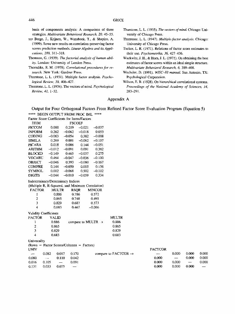
from Equations 5 and 6.1 The unique output for theWISC-III data is presented in Appendix A. As shown,the factor score coefficients (Wt/) are listed first andare followed by indeterminacy indices: (a) the mul-tiple correlation between each factor and the originalvariables, p, as well as its square, p2 (Green, 1976;Mulaik, 1976), and (b) the minimum possible corre-lation between two sets of competing factor scores,2p2 - 1 (Guttman, 1955; Mulaik, 1976; Schonemann,1971). The former index ranges from 0 to 1, with highvalues being desirable, and indicates the maximumpossible degree of determinacy for factor scores thatsatisfy Equation 3. Its square, p2, represents the maxi-mum proportion of determinacy. The second indeter-minacy index ranges from -1 to +1, and high positivevalues are desirable. As discussed previously, when p< .707 (at least 50% indeterminacy), 2p2 - 1 will beless than or equal to 0, meaning that two sets of com-peting factor scores can be constructed for the samecommon factor that are orthogonal or even negativelycorrelated. Values for p that do not appreciably ex-ceed .71 are therefore particularly problematic. Theresults for the first three extracted factors of theWISC-III (see Appendix A) are all above .80 and

1 This program as well as other programs described inthis article can be downloaded from James W. Grice's Website at http://psychology.okstate.edu/faculty/jgrice/factorscores/.

436 GRICE

seem sufficient, but the 2p2 - 1 values are fairly lowand suggest that the best possible factor score esti-mates may still be too indeterminate. The results forthe fourth factor, freedom from distractibility, how-ever, are clear because p is only .683 and 2p2 - 1 is-.066. Such low values indicate that two orthogonalsets of factor scores could be created that are bothequally consistent with the factor loadings. Therefore,refined or coarse factor scores should not be estimatedfor this factor. High degrees of indeterminacy mayalso be an impetus to reexamine the scree plot orfactor-selection criterion and consider extractingfewer factors (see Schb'nemann & Wang, 1972).

The p values represent upper bounds on the deter-minacy of factor score estimates that can be computedfor each of the factors. The refined factor scores thatare actually computed, however, may have lower pro-portions of determinacy. The validity coefficients re-ported next in the output (see Appendix A) providethe means for assessing this possibility. These valuesrepresent the correlations between the factor score es-timates and their respective factors, and may rangefrom -1 to +1. They should be interpreted in the samemanner as p described previously. Gorsuch (1983, p.260) recommends values of at least .80, but muchlarger values (>.90) may be necessary if the factorscore estimates are to serve as adequate substitutes forthe factors themselves. In the present example, thevalidity coefficients are equal to the ps because therefined approach in Equation 5 minimizes the propor-tion of indeterminacy (i.e., it maximizes validity) inthe estimated factor scores. The refined methods inEquations 8, 9, and 10, however, minimize differentfunctions and may therefore produce lower validitiesthat must be scrutinized in relation to p.

Another useful criterion for evaluating factor scoresis univocality, which represents the extent to whichthe estimated factor scores are excessively or insuffi-ciently correlated with other factors in the same analy-sis. As shown in Appendix A, two matrices, labeledUNIV and FACTCOR, are to be compared to assessunivocality. The values in the latter matrix are theinterfactor correlations, which are all 0 for the presentset of orthogonal factors. The values in the formermatrix are the correlations between the refined factorscores (the rows) and the other, noncorrespondingfactors in the analysis (the columns). For example,.082 in the UNIV matrix represents the correlationbetween the second factor and the refined factorscores for the first factor, whereas .080 represents thecorrelation between the first factor and the refined

factor scores for the second factor. The values in theUNIV matrix should match those in the FACTCORmatrix if the estimated factor scores are univocal. Theresults for the WISC-III factors are fairly good be-cause most values are similar across the two matricesand the maximum absolute difference is only .170.These results therefore indicate that the estimated fac-tor scores are not heavily contaminated by variancefrom other orthogonal factors in the same analysis.

The final criterion for evaluating the factor scores iscorrelational accuracy, which indicates the extent towhich the correlations among the estimated factorscores match the correlations among the factors them-selves.2 This criterion can be assessed from the finaltwo matrices shown in Appendix A. The SCORECORmatrix represents the correlations among the refinedfactor scores, and the FACTCOR matrix again repre-sents the correlations among the factors. The esti-mated factor scores reveal superior levels of correla-tional accuracy when the values in the two matricesmatch. In the present example, the correlations amongthe refined factor scores compare favorably with thecorrelations among the four orthogonal factors ex-tracted from the current WISC-III data (see AppendixA). The coefficients for the refined factor scores in theSCORECOR matrix are generally small, and the larg-est difference between the two matrices is for the jointfirst and fourth factors (r = .191).

In summary, the refined factor scores for theWISC-III four-factor orthogonal solution were foundto possess several desirable and undesirable charac-teristics. The multiple correlations, p, appeared ad-equate for three of the factors, but the 2p2 - 1 valuesseemed low. These two indeterminacy indices for the

2 The validity coefficients are taken from the diagonal of^, a matrix of correlations between the / factors and s

factor scores, which is computed as follows:

R — G' \Hl T -1fs — fk kf ss » (12)

where LM is a diagonal matrix of factor score standarddeviations. These values are the square roots of the diagonalelements of Css, which is computed as follows:

ca = (13)

The off-diagonal elements of R/s constitute the values forunivocality (see Gorsuch, 1983, p. 273). The correlationalaccuracy values are computed by calculating the Pearsonproduct-moment correlations among the estimated factorscores.

EVALUATING FACTOR SCORES 437

freedom from distractibility factor, however, wereclearly too low. The validity coefficients matched thep values, and the refined factor scores demonstratedadmirable levels of univocality and correlational ac-curacy for all four factors; that is, the factor scoreswere not overly contaminated with variance fromother orthogonal factors in the same analysis, norwere they highly correlated with one another.

The factor analysis options of the program de-scribed previously can be adjusted to derive obliquefactors. Also, the program itself can be slightly modi-fied to compute refined factor scores on the basis ofEquation 10 rather than on Equation 5. These modi-fications were made to provide another example of theprocess of evaluating indeterminacy, validity, univo-cality, and correlational accuracy (see Footnote 1).Four factors were again extracted, but an oblique,promax transformation was applied to the factors. Thepattern coefficients and factor correlations are pre-sented in Table 2. The loadings could not be com-pared to the WISC-III manual because results foroblique rotations were not reported. It is interesting tonote, however, that the four orthogonal factors from

Table 2Pattern Coefficients and Factor Correlations forPromax-Rotated Factors From the WISC-III

Pattern coefficients

Subtest

Picture CompletionInformationCodingSimilaritiesPicture ArrangementArithmeticBlock DesignVocabularyObject AssemblyComprehensionSymbol SearchDigit Span

1

.108

.739"-.146

.777a

.143

.115-.078

.864a

-.024.553a

.047-.035

2

.616"-.038-.019

.059

.328a

-.112.764a

.018

.822a

-.025-.005

.046

3

.013-.012

.750a

-.084.353.195.020

-.013-.062

.023

.791a

-.168

4

-.014.062

-.010-.101-.049

.510a

.231-.055-.127

.200-.093

.572a

Factor correlations1. Verbal2. Performance3. Processing speed4. FD

—.504.373.556

—.508 —.321 .443 —

Note. Salient structure coefficients (£.30) are in bold. FD =freedom-from-distractibility factor.a Corresponding structure coefficients that were salient in the origi-nal Wechsler Intelligence Scale for Children—Third Edition(WISC-III) standardization sample.

the exploratory analyses were allowed to become cor-related in the confirmatory factor analyses (seeWechsler, 1991, pp. 191-195 and p. 281).

The unique output generated by the evaluation pro-gram for the oblique factors and the refined factorscores is presented in Appendix B. As shown, themultiple correlations for the first three factors aregreater than .87 and deemed adequate. The multiplecorrelation for the fourth factor, although better thanthe corresponding result for the orthogonal factorsreported previously, is marginal (p = .792). The 2p2

- 1 indeterminacy indices are also relatively highcompared with the same values for the orthogonalfactors, but the fourth factor still appears suspect. Thevalidity coefficients for the refined factor scores com-pare favorably with the multiple correlations, with thegreatest loss in validity (.734 compared with .792)occurring for the troubled fourth factor. As stated pre-viously, only refined factor scores computed usingEquation 5 ensure maximum validity. With respect tounivocality, the scores for the oblique factors areagain sufficient. As can be seen in Appendix B, thevalues in the UNIV and FACTCOR matrices arehighly similar. The largest absolute difference isfound for the fourth factor's correlation with the re-fined factor scores for the first factor (.408 comparedwith .556; absolute difference = .148). It is alsoworth mentioning that the correlations between thefactors and the refined factor scores are generallylower than the correlations among the factors, as re-vealed by the lower values in the UNIV matrix com-pared with the FACTCOR matrix. A similar effectcan be seen in terms of correlational accuracy, be-cause the values in the SCORECOR matrix are lessextreme than the values in the FACTCOR matrix. Thecorrelational accuracy of the refined factor scores,however, is sufficient as the SCORECOR and FACT-COR matrices are highly similar. The largest differ-ence is found for the correlation between the first andfourth factors (.374 compared with .556; absolute dif-ference = .182). On the whole, the refined factorscores computed using Equation 10 for the obliquesolution are superior to the scores from the orthogonalsolution reported previously, but the scores for thefourth factor (freedom from distractibility) are stillmarginal at best.

Coarse Factor Scores

The method for computing the four index scores(coarse factor scores) for the WISC-III is based on thestructure coefficients derived from exploratory factor

438 GRICE

analyses of the original standardization sample. Forexample, the Information, Similarities, Vocabulary,and Comprehension subtests were found to possesssalient, positive structure coefficients (>.30) on thefirst factor, labeled as verbal comprehension, for anorthogonally rotated four-factor solution. Scores onthese subtests are therefore summed to create thecoarse factor score for any given child who completesthe WISC-III. Because the subtests are all on thesame scale, it is not necessary to standardize the databefore performing this computation. As stated previ-ously, the structure coefficients from orthogonal fac-tors for the present group of children diagnosed withlearning disabilities (see Table 1) match the WISC-IIIstandardization sample quite well. Consequently, thespecific procedures for summing the subtest scoresinto coarse factor scores found in the WISC-IIImanual were initially followed here, and the resultingscores were assessed using a SAS IML evaluationprogram (see Footnote 1).

The novel output generated from this program isreported in Appendix C. As shown, the matrix ofwhole weights used to create the coarse factor scoresis listed first. This matrix is essentially a simplifiedfactor score coefficient matrix, and examination of itscolumns reveals how the items are summed to com-pute the scores for each factor. For example, scores onthe third factor are computed by summing the Codingand Symbol Search subtests. Because all of the non-zero weights are positive, no subtests are subtracted inthe present scoring scheme. The indeterminacy indi-ces—p, p2, and 2p2 - 1—are reported next to providea basis of comparison. Validity coefficients for thecoarse factor scores are then listed and compared withthe multiple correlations for the factors. Because thecoarse factor scores entail a loss of information, theirvalidity coefficients will most assuredly be less thanthe ps, and the goal is to achieve as little discrepancybetween the values as possible. The results in Appen-dix C reveal that the coarse factor scores for the fourthfactor are clearly inadequate (which is necessarily thecase given the low multiple correlation), and thescores for the second factor compare least favorablywith their respective multiple correlation (difference= .064). Univocality follows the validity informationand reveals that the coarse factor scores are only mod-estly contaminated by other orthogonal factors in theanalysis (maximum = .293). The correlational accu-racy matrix, however, reveals moderate overlapamong several coarse factor scores. The scores on thesecond factor, for instance, correlate .457 and .414

with scores on the first and third factors, respectively.Hence, even though the factors themselves are uncor-related, several of the coarse factor scores are mod-erately oblique. In summary, the validity indices re-veal that the coarse factor scores for the fourth factor(freedom from distractibility) are clearly inadequate.Validity coefficients for the first three factors appearadequate, but attempts to improve the coarse factorscores for the second factor (i.e., trying different setsof weights) might be fruitful. This latter suggestion issupported by several poor correlational accuracy val-ues for the second factor.

The method for deriving the unit-weighted, coarsescoring scheme used in the WISC-III (i.e., determin-ing how to weight the items on the basis of the struc-ture coefficients) is common in practice and widelyendorsed in the literature (Alwin, 1973; Gorsuch,1997; ten Berge & Knol, 1985). Two recent MonteCarlo studies conducted by Grice and Harris (1998)and Grice (2001), however, suggest that the simplifiedscoring scheme should be based on the factor scorecoefficients instead. These coefficients are designedexplicitly for determining the relative spacings of theindividuals on the factors and are computed usingleast squares methods that can maximize the determi-nate nature of the estimated factor scores (viz., Equa-tion 5), whereas the structure coefficients simply rep-resent the correlations between the items and thefactors. The relative values in these two matrices willtypically correspond when ideal simple structure isobtained, which is certainly the exception rather thanthe rule in practice. It is therefore entirely possiblethat using the structure coefficients to determine itemsaliency for scoring one's factors may result in coarsefactor scores that have poor validity, univocality, andcorrelational accuracy. This potentiality may explainthe poor performance of the coarse scores for the sec-ond factor described previously relative to the firstand third factors.

A SAS IML program was written that provides themeans for selecting salient items from the factor scorecoefficients (see Footnote 1). The output generatedfrom this program for the current WISC-III data isreported in Appendix D. As shown, the factor scorecoefficients for the first factor are initially ranked indescending order. These ranked values are then plot-ted in a two-dimensional graph with the abscissa com-prising the ranks and the ordinate comprising the fac-tor score coefficients. As can be seen in the top panelof Figure 1, the resulting graph is similar to a screeplot. A clear break in the graph is present that sepa-

EVALUATING FACTOR SCORES 439

Ranked Factor Score Coefficients: Factor 1

M

.1o

JEo0o<ooo

V)

2u.

0.5

0.4

0.3

0.2

0.1

0.0

-0.1

-0.2

VOCABU

SIMILAjupoRM

-

COMPRE

-

- PIC^™EO№ICC°^ITHM

DIGIT£DBJECT

-

BLOCKD1 1 1 1 1 1 1 1 1 1 1 1

1 2 3 4 5 6 7 8 9 10 11 12

Ranked Factor Score Coefficients: Factor 2

&C.2'o£Q>Oo

oo(0L.,0

LL.

0.5

0.4

0.3

0.2

0.1

0.0

-0.1

-0.2

—BLOCKD

OBJECT

-

PICCOM

PICARA

SIMILA, s

VOCABICOMPRB:

ARITHM

I I I I I I 1 I I I I I

1 2 3 4 5 6 7 8 9 10 11 12

Rank

Figure 1. Plots of ranked factor score coefficients (Equation 5) for first and second or-thogonal factors. Abbreviations for subtests are as follows: VOCABU = Vocabulary;SIMILA = Similarities; INFORM = Information; COMPRE = Comprehension; PICARA= Picture Arrangement; SYMBOL = Symbol Search; PICCOM = Picture Completion;ARITHM = Arithmetic; DIGITS = Digit Span; OBJECT = Object Assembly; CODING =Coding; BLOCKD = Block Design.

440 GRICE

rates Vocabulary, Similarities, Information, and Com-prehension from the remaining subtests on the firstfactor. Moreover, a second break in the graph revealsa particularly extreme negative factor score coeffi-cient for Block Design. The coarse factor scores arehence computed by summing Vocabulary, Similari-ties, Information, and Comprehension, and subtract-ing Block Design. This method differs from the origi-nal scoring procedure reported in the WISC-IIImanual by including the Block Design subtest. Thegraph of ranked factor score coefficients for the sec-ond factor is presented in the bottom panel of Figure1 and reveals that the coarse factor scores should becomputed by summing Block Design, Object Assem-bly, and Picture Completion. Unlike the original scor-ing procedure, the Picture Arrangement subtest is notincluded for the second factor. It should also be notedthat although Picture Arrangement shows slight sepa-ration from Similarities in the graph, its absolutevalue is similar to Arithmetic, which shows virtuallyno separation from Symbol Search and a number ofother subtests. Including Picture Arrangement wouldtherefore justify including these other negativelyweighted subtests as well. As with interpreting a tra-ditional scree plot, a degree of subjectivity is obvi-ously involved. Unlike a scree test, however, the re-searcher can use the evaluation program describedpreviously to assess the adequacy of the coarse factorscores and make adjustments if necessary. Accordingto the scree-type plot for the third factor (not shown),coarse factor scores are computed from the Codingand Symbol Search subtests, which matches the origi-nal scoring scheme. Coarse factor scores for thefourth factor are computed by summing the Arithme-tic, Block Design, Comprehension, and Digit Spansubtests, and subtracting the Object Assembly subtest.In the original scoring scheme, only the Arithmeticand Digit Span subtests are summed. It is interestingto note that the troubled fourth factor produced a plot(not shown) that did not reveal clear separation amongthe factor score coefficients, which more than doubledthe number of subtests used to estimate the factorscores.

Standard errors and t values for the factor scorecoefficients are also listed in the output (see AppendixD).3 A common criticism against least squares regres-sion weights (e.g., see Gorsuch, 1997) is the potentialfor wildly different standard errors that would obscurethe interpretation of their relative magnitudes. Basingthe coarse factor scoring scheme on such coefficientswould therefore be risky business. The results for this

particular data set, however, reveal that the standarderrors within each factor are fairly homogeneous, andthe most extreme t values correspond to the mostextreme factor score coefficients. For example, thePicture Completion (5.57), Block Design (10.53), andObject Assembly (9.84) subtests clearly have the mostextreme t values (listed in parentheses) for the secondfactor. The t value for Picture Arrangement (2.23) onthe second factor was not unusual, justifying its ex-clusion from the coarse factor scores. Hence, the stan-dard errors and t values support the weightingschemes for computing the factor scores derived fromthe graphs in Figure 1. The output concludes with thetotal contribution of each item (WISC-III subtest) tothe squared multiple correlation, p2, for each factor.4

The factor score coefficients represent the direct con-tribution of each item to p2, whereas the numbers inthis final matrix include both direct and indirect ef-fects. These values can consequently be examined todetermine whether additional items need to be in-cluded in the computation of the coarse factor scores.In this data set, the largest values correspond to thelargest factor score coefficients for each factor, andhence no additional items are deemed necessary.

These new coarse factor scores based on the factorscore coefficients for the orthogonal four-factor solu-tion were evaluated using the program described pre-viously. The results are reported in Appendix E andcan be compared with the original output based on thestructure coefficients in Appendix C. This comparisonreveals that the validity coefficients for the first andsecond factors were improved by the adjustments.The first factor increased from .852 to .864 (p =.886), and the second factor improved from .801 to.831 (p = .865). The new coarse factor scores for thebeleaguered fourth factor, however, showed little im-provement (.627 to .629), although the changes were

3 The standard error for the factor score coefficient ofItem / and Factor j was computed as follows:

- Rj)/N - * - I)1 (14)

where ri; is the fth main diagonal entry of the inverse of theitem correlation matrix, RJ is the squared validity coeffi-cient for Factor j (not p2), N is the total number of obser-vations, and k is the number of items (see Harris, 1985b,p. 65).

4 The total direct and indirect contributions to the squaredmultiple correlations for the factors were computed usingelement-wise multiplication of the structure and factor scorecoefficient matrices.

EVALUATING FACTOR SCORES 441

in vain given the already inadequate multiple corre-lation (p = .683). The validity coefficient for the thirdfactor did not change because the scoring schemesbased on the structure and factor score coefficientswere equivalent in this case. Comparison of the univ-ocality matrices in Appendices E and C also revealimprovement, as values in the former Appendix aregenerally closer to the comparison matrix of zeros. Inother words, the new coarse factor scores are lesscontaminated by other factors in the same analysis.The exception to this general improvement involvesthe fourth factor. The new coarse factor scores showmore contamination from the fourth factor than fromthe original scores. This result is not completely sur-prising, however, given that two of the three itemsadded to this factor are shared by other factors in theanalysis. Finally, a comparison of the correlationalaccuracy matrices across Appendices E and C againshows improvement for the correlations involvingonly the first three factors and a decrement in perfor-mance for the fourth factor. The correlations amongthe new coarse factor scores for the first three factorsresembles the comparison matrix (in this case, anidentity matrix) more closely than the original coarsefactor scores.

In summary, the coarse factor scores based on thefactor score coefficients revealed superior levels ofvalidity, univocality, and correlational accuracy forthe first three factors compared with the originalscores based on the structure coefficients. The coarsefactor scores for the fourth factor showed a slightimprovement in validity but decrements in univocalityand orthogonality. It should be kept in mind, however,that the fourth factor was retained in all of the analy-ses to provide a thread of consistency throughout theexamples. It was therefore retained solely for peda-gogical reasons. Given all of the results stated previ-ously for both the refined and coarse factor scoringmethods, a more appropriate strategy may have beento reconduct the factor analyses and extract only threefactors, or retain four factors and apply an obliquetransformation. Even with oblique factors, the fourthfactor was marginal, as revealed by its indeterminacyindices, and the best alternative may consequently beits exclusion.

Discussion

Factor scores computed from the common factormodel are indeterminate in nature. For any singlecommon factor, an infinite number of sets of scorescan be derived that are equally consistent with the

factor loadings. Under particular circumstances, com-peting sets of scores for the same factor can actuallybe orthogonal or negatively correlated, thus yieldingcompletely different rankings of the individuals. Thisinherent indeterminacy creates both conceptual(Steiger & Schonemann, 1978) and empirical(Schonemann & Steiger, 1978; Steiger, 1979) diffi-culties for the factor analyst that should not be ig-nored. Indeterminacy has also led to a large number ofmethods for estimating factor scores, some of whichappear to be defective. In other words, not all meansof calculating factor scores are adequate; hence, evenif highly determinate factor scores can be created fora given set of results, the researcher may still choosea method that is severely flawed (e.g., summing stan-dardized scores on the basis of salient structure coef-ficients). The foregoing procedures and computer pro-grams were specifically designed to provideresearchers with the knowledge and tools necessaryfor effectively addressing, rather than neglecting, theissues surrounding the computation of factor scoreestimates. The structure and style by which this in-formation was presented was intentionally pedagogi-cal, introducing and demonstrating procedures andcriteria for evaluating factor scores that are unknownto a vast majority of researchers and consumers offactor analytic technology. A number of differentquestionnaires, inventories, or ability tests other thanthe WISC-III (Wechsler, 1991) could certainly havebeen chosen for this purpose, as the evaluative com-puter programs were designed for maximum flexibil-ity. Large numbers of items and factors, different fac-tor extraction algorithms, and orthogonal or obliquefactor transformations can all be managed by the com-puter programs reported in this article.

Choosing the WISC-III for the previously de-scribed demonstrations, however, proved fortuitousfor a number of reasons. First, it is a widely usedassessment tool in psychology and education and istherefore familiar to a large and diverse audience ofreaders. Second, it possesses a number of manageableitems (subtests) that could be displayed and discussedefficiently. Finally, and most importantly, a good dealof controversy surrounds the validity of the four-factor solution reported in the test manual. Some re-searchers have argued that a two- or three-factor so-lution provides superior fit to the extant data,directing most of their criticism toward the freedomfrom distractibility factor (Kamphaus, Benson, Hutch-inson, & Platt, 1994; Kush & Watkins, 1994; Saltier,1992). The results reported previously may therefore

442 GRICE

be interpreted in light of a genuine measurement con-troversy, further exhibiting the importance of factorscore indeterminacy. Viewed in this light, the freedomfrom distractibility factor was clearly inadequate. Itsmultiple correlation, p, was less than .707, and theminimum correlation among competing sets of factorscores, 2p2 - 1, was -.066. Because the multiple cor-relation was low, the validity coefficient for thecoarse factor scores (index scores) was necessarilylow as well. Applying an oblique transformation tothe extracted factors improved the multiple correla-tion (p = .792), but it was still inadequate.

In a recent article, Fabrigar et al. (1999) offered anumber of recommendations to aid researchers withthe various decisions that must be made when con-ducting an exploratory factor analysis (EFA). Sadly,they did not recommend evaluating factor score inde-terminacy or the adequacy of one's computed factorscore estimates. The example reported previously forthe WISC-III, however, demonstrates clearly the ne-cessity for incorporating such evaluations into anyEFA. Even if the researcher will not finally computefactor scores for his or her data, the maximum pro-portion of determinacy for each factor, p2, should atleast be reported along with the eigenvalues, rotationmethod, and structure or pattern coefficients that areroutinely published. SAS reports p if the factor scorecoefficients are requested, and SPSS reports p for or-thogonal factors if factor scores from Equation 5 (la-beled as regression factor scores in the program) arerequested. None of the commercial programs, how-ever, provide the means for computing factor scoresfrom Equations 5, 8, 9, and 10. For instance, SASallows one to compute refined factor scores usingEquation 5, and SPSS provides options for computingrefined factor scores from Equations 5, 7, and 9. Thenecessary tools for evaluating refined as well ascoarse factor scores in terms of validity, univocality,and correlational accuracy are not available. More-over, although most major programs provide thestructure, pattern, and factor score coefficients fromEquation 5, they do not provide the graphical dis-plays, t values, and standard errors for the factor scorecoefficients, W^ nor do they provide the combineddirect and indirect contributions of each item to p2.The programs reported in this article should thereforeprove vital to EFA researchers for constructing andevaluating factor score estimates as well as the degreeof indeterminacy in their analyses.

If factor scores are computed for a particular set ofresults, or a method of computing factor scores is

provided for future researchers using the same instru-ment (e.g., as in scale construction), then informationregarding the validity, univocality, and correlationalaccuracy of the factor score estimates should be re-ported. Validity represents the extent to which thefactor score estimates correlate with their respectivefactors in the sample, and values approaching 1.00 aredesirable. Low validity will likely reduce the statisti-cal power of subsequent decisions based on the factorscores because a large proportion of their variancemay be random in nature. Validity must also bejudged, however, within the context of univocalityand correlational accuracy because a small decrementin the former index may correspond with substantiallosses in the latter indices. As a consequence, thefactor score estimates may become overly saturatedwith variation from other factors and factor score es-timates in the same analysis. Such an outcome couldconfound the process of interpreting the relationshipsbetween factor score estimates for a particular factorand external criteria. For example, consider a re-searcher who extracts two orthogonal factors, labelsthem as depression and hostility, uses a scoringmethod that produces highly correlated factor scoreestimates, and then fails to evaluate the scores forvalidity, univocality, and correlational accuracy. Sub-sequent analyses will all be interpreted in light oforthogonal factors, even though the factor score esti-mates themselves are not independent. All threeevaluative criteria should therefore be carefully ex-amined and reported as standard output of any EFA.

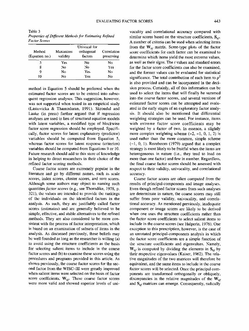
When factor scores are computed and evaluated, achoice between refined or coarse factor score esti-mates must be made. Refined factor scores will typi-cally have superior levels of validity compared withtheir coarse counterparts for a given sample, and par-ticular constraints, such as orthogonality for uncorre-lated factors, can be placed on these scores. Conse-quently, if one wishes to employ a complex weightingscheme that uses all of the items, the refined factorscores would be suitable. The researcher will have todecide, however, what constraints are to be employed.Table 3 serves as a quick summary of the differentproperties of the factor score estimates generated fromEquations 5, 8, 9, and 10. As shown, each methodfails to meet all three criteria, and the methods inEquations 9 and 10 only ensure univocality when thefactors are orthogonal. Some authors have addition-ally argued that the purposes for which factor scoresare to be used should be included in one's choice. Forexample, Tucker (1971) showed analytically that the

EVALUATING FACTOR SCORES 443

Table 3Properties of Different Methods for Estimating RefinedFactor Scores

Method(Equation no.)

589

10

Maximizesvalidity

YesNoNoNo

Univocal fororthogonal

factors

NoNoYesYes

Correlationpreserving

NoYesNoNo

method in Equation 5 should be preferred when theestimated factor scores are to be entered into subse-quent regression analyses. This suggestion, however,was not supported when tested in an empirical study(Lastovicka & Thamodaran, 1991). Skrondal andLaake (in press) further argued that if regressionanalyses are used in lieu of structural equation modelswith latent variables, a modified type of blockwisefactor score regression should be employed. Specifi-cally, factor scores for latent explanatory (predictor)variables should be computed from Equation 5,whereas factor scores for latent response (criterion)variables should be computed from Equations 9 or 10.Future research should add to this store of knowledgein helping to direct researchers in their choice of therefined factor scoring methods.

Coarse factor scores are extremely popular in theliterature and go by different names, such as scalescores, index scores, cluster scores, and sum scores.Although some authors may object to naming suchquantities factor scores (e.g., see Thorndike, 1978, p.321), the values are intended to provide the rankingsof the individuals on the identified factors in theanalysis. As such, they are justifiably called factorscores (estimates) and are generally believed to besimple, effective, and stable alternatives to the refinedmethods. They are also considered to be more con-sistent with the process of factor interpretation, whichis based on an examination of subsets of items in theanalysis. As discussed previously, these beliefs maybe well founded as long as the researcher is willing (a)to avoid using the structure coefficients as the basisfor selecting salient items to include in the coarsefactor scores and (b) to examine these scores using theprocedures and programs provided in this article. Asshown previously, the coarse factor scores for the sec-ond factor from the WISC-III were greatly improvedwhen salient items were selected on the basis of factorscore coefficients, W^. These coarse factor scoreswere more valid and showed superior levels of uni-

vocality and correlational accuracy compared withsimilar scores based on the structure coefficients, S .̂A number of criteria can be used when selecting itemsfrom the W^- matrix. Scree-type plots of the factorscore coefficients for each factor can be examined todetermine which items yield the most extreme values,as well as their signs. The t values and standard errorsfor the factor score coefficients can also be examined,and the former values can be evaluated for statisticalsignificance. The total contribution of each item to p2

is also provided and can be incorporated in the deci-sion process. Certainly, all of this information can beused to select the items that will finally be summedinto the coarse factor scores, and several versions ofestimated factor scores can be attempted and evalu-ated in the early stages of an exploratory factor analy-sis. It should also be mentioned that differentialweighting strategies can be used. For instance, itemswith extreme factor score coefficients may beweighted by a factor of two. In essence, a slightlymore complex weighting scheme (—2, — 1, 0, 1, 2) isused rather than the more common, simple scheme(-1, 0, 1). Rozeboom (1979) argued that a complexstrategy is most likely to be fruitful when the items areheterogeneous in nature (i.e., they tend to load onmore than one factor) and few in number. Regardless,the final coarse factor scores should be assessed withrespect to their validity, univocality, and correlationalaccuracy.

Coarse factor scores are often computed from theresults of principal-components and image analyses.Even though refined factor scores from such analysesare determinate in nature, the coarse scores may stillsuffer from poor validity, univocality, and correla-tional accuracy. As mentioned previously, inadequatecomponent or image scores are likely to be derivedwhen one uses the structure coefficients rather thanthe factor score coefficients to select salient items toinclude in the coarse scores (see Halperin, 1976). Oneexception to this prescription, however, is the case ofan unrotated principal-components analysis in whichthe factor score coefficients are a simple function ofthe structure coefficients and eigenvalues. Namely,Wty is computed by dividing the elements in S^ bytheir respective eigenvalues (Kaiser, 1962). The rela-tive magnitudes of the two matrices will therefore beequivalent, and the same items to include in the coarsefactor scores will be selected. Once the principal com-ponents are transformed orthogonally or obliquely,discrepancies in the relative magnitudes of the W^and Skf matrices can emerge. Consequently, radically

444 GRICE

different coarse factor scores can be derived (Harris,1985a, 1985b). Because the factor score coefficientsare designed specifically for scoring the components,and the structure coefficients represent the correla-tions between the components and the items, theformer values will yield coarse factor scores that havesuperior levels of validity, univocality, and correla-tional accuracy compared with the latter.

In conclusion, many early psychologists believedthat the common factor model and exploratory factoranalytic techniques would help shape our understand-ing of human abilities and individual differences.Support for these beliefs can indeed be seen in mod-ern theories of intelligence, personality, and self-esteem, to name only a few domains or constructs thathave been modeled with factor analysis. Critics haveargued, however, that factor score indeterminacy se-riously hinders the effectiveness of the common factormodel and may in fact render it misleading (e.g., seeSchonemann, 1997; Schonemann & Wang, 1972;Steiger, 1996b) or even meaningless (see Schone-mann & Steiger, 1978). The question posed by mostcritics is: Of what scientific value is a common factorif the researcher cannot score the individuals in anunambiguous fashion along the identified dimension?For instance, imagine a measure of temperature thathas a high degree of factor score indeterminacy. Tworesearchers could use such a measure to derive com-pletely different rankings, both equally valid, of thetemperatures in the rooms of their buildings. It is dif-ficult to imagine that such a measure would bedeemed as adequate or would propel the science oftemperature forward. Yet, this is exactly the issue fac-ing psychologists who use exploratory factor analysistechniques and fail to evaluate factor score indetermi-nacy or their estimated factor scores. Thurstone's(1935) attempt to separate the factor identification andscoring processes may be at the root of this dilemma,but as Steiger (1996a) recently wrote, "If we wish tocontinue using models with more latent than observedvariables, we need to discuss and develop methods forthe measurement and evaluation of factor indetermi-nacy, so that the problem is properly controlled" (p.619). The present article provides researchers andpractitioners with these much needed methods.

References

Alwin, D. F. (1973). The use of factor analysis in the con-struction of linear composites in social research. Socio-logical Methods & Research, 2, 191-213.

Anderson, R. D., & Rubin, H. (1956). Statistical inferencein factor analysis. Proceedings of the Third BerkeleySymposium of Mathematical Statistics and Probability, 5,111-150.

Bartlett, M. S. (1937). The statistical conception of mentalfactors. British Journal of Psychology, 28, 97-104.

Burt, C. (1940). The factors of mind. London: London Uni-versity Press.

Cattell, R. B. (1952). Factor analysis: An introduction andmanual for the psychologist and social scientist. NewYork: Harper.

Comrey, A. L. (1978). Common methodological problemsin factor analytic studies. Journal of Consulting andClinical Psychology, 46, 648-659.

Costa, P. T., Jr., & McCrae, R. R. (1992). Revised NEOPersonality Inventory (NEO-PI-R) and NEO Five-Factor Inventory (NEO-FFI) professional manual.Odessa, FL: Psychological Assessment Resources.

Fabrigar, L., Wegener, D., MacCallum, R., & Strahan, E.(1999). Evaluating the use of exploratory factor analysisin psychological research. Psychological Methods, 4,272-299.

Garnett, J. C. M. (1919a). General ability, cleverness andpurpose. British Journal of Psychology, 9, 345-366.

Garnett, J. C. M. (1919b). On certain independent factors inmental measurements. Proceedings of the Royal Society,Series A, 96, 91-111.

Gorsuch, R. L. (1983). Factor analysis (2nd ed.). Hillsdale,NJ: Erlbaum.

Gorsuch, R. L. (1997). Exploratory factor analysis: Its rolein item analysis. Journal of Personality Assessment, 68,532-560.

Green, B. F. (1976). On the factor score controversy. Psy-chometrika, 41, 263-266.

Grice, J. W. (2001). A comparison of factor scores underconditions of factor obliquity. Psychological Methods, 6,67-83.

Grice, J. W., & Harris, R. J. (1998). A comparison of re-gression and loading weights for the computation of fac-tor scores. Multivariate Behavioral Research, 33, 221-247.

Grice, J. W., Krohn, E. J., & Logerquist, S. (1999). Cross-validation of the WISC-III factor structure in twosamples of children with learning disabilities. Journal ofPsychoeducational Assessment, 17, 236-248.

Guttman, L. (1955). The determinacy of factor score matri-ces with applications for five other problems of commonfactor theory. British Journal of Statistical Psychology, 8,65-82.

EVALUATING FACTOR SCORES 445

Halperin, S. (1976). The incorrect measurement of compo-nents. Educational and Psychological Measurement, 36,347-353.

Harman, H. H. (1976). Modern factor analysis (3rd ed.).Chicago: University of Chicago Press.

Harris, R. J. (1985a, November). Further features of a fac-tor fable. Paper presented at the annual meeting of theSociety for Multivariate Psychology, Berkeley, CA.

Harris, R. J. (1985b). A primer of multivariate statistics(2nd ed.). Orlando, FL: Academic Press.

Heermann, E. F. (1963). Univocal or orthogonal estimatorsof orthogonal factors. Psychometrika, 28, 161-172.

Holzinger, K. J., & Harman, H. H. (1941). Factor analysis.Chicago: University of Chicago Press.

Horn, J. L. (1965). An empirical comparison of methods forestimating factor scores. Educational and PsychologicalMeasurement, 25, 313-322.

Kaiser, H. F. (1962). Formulas for component scores. Psy-chometrika, 27, 83-87.

Kamphaus, R. W., Benson, J., Hutchinson, S., & Platt, L. O.(1994). Identification of factor models for the WISC-III.Educational and Psychological Measurement, 54, 174—186.

Kestelman, H. (1952). The fundamental equations of factoranalysis. British Journal of Psychology, 5, 1-6.

Kush, J. C., & Watkins, M. W. (1994). Factor structure ofthe WISC-III for Mexican-American, learning disabledstudents (Clearing House No. TM 022 083). East Lan-sing, MI: National Center for Research on Teacher Learn-ing. (ERIC Document Reproduction Service No. ED 374154)

Lastovicka, J., & Thamodaran, K. (1991). Common factorscore estimates in multiple regression problems. Journalof Marketing Research, 28, 105-112.

Ledermann, W. (1939). On a shortened method of estima-tion of mental factors by regression. Psychometrika, 4,109-116.

Lovie, P., & Lovie, A. D. (1995). The cold equations:Spearman and Wilson on factor indeterminacy. BritishJournal of Mathematical and Statistical Psychology, 48,237-253.

Maraun, M. D. (1996). Metaphor taken as math: Indetermi-nacy in the factor analysis model. Multivariate Behavior-al Research, 31, 517-538.

McDonald, R. P. (1974). The measurement of factor inde-terminacy. Psychometrika, 39, 203-222.

McDonald, R. P. (1981). Constrained least squares estima-tors of oblique common factors. Psychometrika, 46, 337-341.

McDonald, R. P., & Burr, E. J. (1967). A comparison of

four methods of constructing factor scores. Psycho-metrika, 32, 381^01.

Meyer, E. P. (1973). On the relationship between ratio ofnumber of variables to number of factors and factorialdeterminacy. Psychometrika, 38, 375-378.

Morris, J. D. (1980). The predictive accuracy of full-rankvariables vs. various types of factor scores: Implicationsfor test validation. Educational and Psychological Mea-surement, 40, 389-396.

Mulaik, S. A. (1972). The foundations of factor analysis.New York: McGraw-Hill.

Mulaik, S. A. (1976). Comments on "The measurement offactorial indeterminacy." Psychometrika, 41, 249-262.

Rozeboom, W. W. (1979). Sensitivity of a linear compositeof predictor items to differential item weighting. Psy-chometrika, 44, 289-296.

Saltier, J. (1992). Assessment of children: WISC-III andWPPSI-R supplement. San Diego, CA: Author.

Schonemann, P. H. (1971). The minimum average correla-tion between equivalent sets of uncorrelated factors. Psy-chometrika, 36, 21-30.

Schonemann, P. H. (1997). On models and muddles of heri-tability. Genetica, 99, 97-108.

Schonemann, P. H., & Steiger, I. H. (1978). On the validityof indeterminate factor scores. Bulletin of the Psycho-nomic Society, 12, 287-290.

Schonemann, P. H., & Wang, M. M. (1972). Some new re-sults on factor indeterminacy. Psychometrika, 37, 61-91.

Skrondal, A., & Laake, P. (in press). Regression amongfactor scores. Psychometrika.

Spearman, C. (1904). 'General intelligence' objectively de-termined and measured. American Journal of Psychol-ogy, 5, 201-293.

Spearman, C. (1927). The abilities of man, their nature andmeasurement. New York: Macmillan.

Spearman, C. (1932). The abilities of man (2nd Impression).London: Macmillan.

Steiger, J. H. (1979). The relationship between externalvariables and common factors. Psychometrika, 44, 93-97.

Steiger, J. H. (1996a). Coming full circle in the history offactor indeterminacy. Multivariate Behavioral Research,31, 617-630.

Steiger, J. H. (1996b). Dispelling some myths about factorindeterminacy. Multivariate Behavioral Research, 31,539-550.

Steiger, J. H., & Schonemann, P. H. (1978). A history offactor indeterminacy. In S. Shye (Ed.), Theory construc-tion and data analysis (pp. 136-178). Chicago: Univer-sity of Chicago Press.

ten Berge, J., & Knol, D. (1985). Scale construction on the

446 GRICE

basis of components analysis: A comparison of threestrategies. Multivariate Behavioral Research, 20, 45-55.

ten Berge, J., Krijnen, W., Wansbeek, T., & Shapiro, A.(1999). Some new results on correlation-preserving factorscores prediction methods. Linear Algebra and its Appli-cations, 289, 311-318.

Thomson, G. (1939). The factorial analysis of human abil-ity. London: University of London Press.

Thorndike, R. M. (1978). Correlational procedures for re-search. New York: Gardner Press.

Thurstone, L. L. (1931). Multiple factor analysis. Psycho-logical Review, 38, 406-427.

Thurstone, L. L. (1934). The vectors of mind. PsychologicalReview, 41, 1-32.

Thurstone, L. L. (1935). The vectors of mind. Chicago: Uni-versity of Chicago Press.

Thurstone, L. L. (1947). Multiple-factor analysis. Chicago:University of Chicago Press.

Tucker, L. R. (1971). Relations of factor score estimates totheir use. Psychometrika, 36, 427-436.

Wackwitz, J. H., & Horn, J. L. (1971). On obtaining the bestestimates of factor scores within an ideal simple structure.Multivariate Behavioral Research, 6, 389-408.

Wechsler, D. (1991). WISC-III manual. San Antonio, TX:Psychological Corporation.

Wilson, E. B. (1928). On hierarchical correlational systems.Proceedings of the National Academy of Sciences, 14,283-291.

Appendix A

Output for Four Orthogonal Factors From Refined Factor Score Evaluation Program (Equation 5)**** BEGIN OUTPUT FROM PROC IML ****Factor Score Coefficients for Items/Factors

ITEM FSCOEFPICCOMINFORMCODINGSIMILAPICARAARITHMBLOCKDVOCABUOBJECTCOMPRESYMBOLDIGITS

0.0000.262

-0.0630.2690.018

-0.012-0.149

0.464-0.046

0.1440.002

-0.044

0.219-0.062-0.054

0.0010.086

-0.0910.465

-0.0470.393

-0.050-0.068-0.010

-0.021-0.018

0.382-0.062

0.1440.091

-0.037-0.036-0.080

0.0050.502

-0.059

-0.0370.053

-0.008-0.107-0.051

0.3820.275

-0.100-0.167

0.156-0.102

0.334

Indeterminacy/Determinacy Indices(Multiple R, R-Squared, and Minimum Correlation)FACTOR MULTR RSQR MINCOR

0.786 0.5720.748 0.4950.687 0.3730.467 -0.066

1234

0.8860.8650.8290.683

Validity CoefficientsFACTOR VALID

1234

0.8860.8650.8290.683

MULTRcompare to MULTR -> 0.886

0.8650.8290.683

Univocality(Rows = Factor Scores/Columns = Factors)UNIV

— 0.082 0.017 0.170 compare to FACTCOR0.110 0.0420.080

0.0160.131

0.1050.033

— 0.0910.075 —

FACTCOR

0.0000.0000.000

0.000 0.000 0.000— 0.000 0.000

0.000 — 0.0000.000 0.000 —

EVALUATING FACTOR SCORES 447

Correlational AccuracySCORECOR

1.000 —0.093 1.0000.019 0.1270.191 0.048

compare to FACTCOR

1.0000.109 1.000

FACTCOR1.0000.0000.0000.000

1.000 —0.000 1.0000.000 0.000 1.000

Appendix B

Output for Four Oblique Factors From Refined Factor Score Evaluation Program (Equation 10)**** BEGIN OUTPUT FROM PROC IML ****Factor Score Coefficients for Items/Factors

ITEM FSCOEFPICCOMINFORMCODINGSIMILAPICARAARITHMBLOCKDVOCABUOBJECTCOMPRESYMBOLDIGITS

0.0420.324

-0.0490.3420.0670.043

-0.0480.381

-0.0180.2390.039

-0.033

0.348-0.029-0.021

0.0270.179

-0.0690.4330.0010.467

-0.021-0.015

0.027

0.0010.0100.539

-0.0530.2500.1800.0170.003

-0.0660.0420.567

-0.084

-0.0230.0680.041

-0.165-0.048

0.7180.322

-0.098-0.182

0.266-0.076

0.783

Indeterminacy/Determinacy Indices(Multiple R, R-Squared, and Minimum Correlation)FACTOR MULTR RSQR MINCOR

1 0.929 0.862 0.7242 0.911 0.830 0.6603 0.876 0.768 0.5364 0.792 0.627 0.253

Validity CoefficientsFACTOR VALID

0.9200.8980.862

compare to MULTR —»

0.734

MULTR0.9290.9110.8760.792

Univocality(Rows :

UNIV

—0.4640.3430.511

= Factor

0.453—

0.4560.288

Scores/Columns = Factors)

0.3220.438

—0.382

0.4080.2360.325

—

compare to FACTCOR ->FACTCOR

0.5050.3730.556

0.505 0.373 0.556— 0.508 0.321

0.508 — 0.4430.321 0.443 —

Correlational AccuracySCORECOR

1.000 —0.418 1.0000.304 0.3900.374 0.196

compare to FACTCOR ->

1.0000.299 1.000

FACTCOR1.000 — —0.505 1.000 —0.373 0.508 1.0000.556 0.321 0.443 1.000

448 GRICE

Appendix C

Output for Four Orthogonal Factors From Coarse Factor Score Evaluation Program**** BEGIN OUTPUT FROM PROC IML ****Simplified Weights for Items/Factors

ITEM FSCOEFPICCOM 0 1 0 0INFORM 1 0 0 0CODING 0 0 1 0SIMILA 1 0 0 0PICARA 0 1 0 0ARITHM 0 0 0 1BLOCKD 0 1 0 0VOCABU 1 0 0 0OBJECT 0 1 0 0COMPRE 1 0 0 0SYMBOL 0 0 1 0DIGITS 0 0 0 1

Indeterminacy/Determinacy Indices(Multiple R, R-Squared, and Minimum Correlation)

FACTOR MULTR RSQR MINCOR1 0.886 0.786 0.5722 0.865 0.748 0.4953 0.829 0.687 0.3734 0.683 0.467 -0.066

compare to MULTR ->

Validity CoefficientsFACTOR VALID

1 0.8522 0.8013 0.8054 0.627

Univocality(Rows = Factor Scores/Columns = Factors)UNIV

MULTR0.8860.8650.8290.683

—0.2200.1020.224

0.263—

0.2930.111

0.0700.192

—0.070

0.2540.0560.170

—

compare to FACTCOR ->

Correlational AccuracySCORECOR

1.000 —0.457 1.0000.200 0.4140.388 0.227

compare to FACTCOR

1.0000.211 1.000

FACTCOR

0.0000.0000.000

FACTCOR1.0000.0000.0000.000

0.000 0.000 0.000— 0.000 0.000

0.000 — 0.0000.000 0.000 —

1.000 —0.000 1.0000.000 0.000 1.000

Appendix D

Output for Four Orthogonal Factors From Program for Creating Coarse Factor Scores (Equation 5)**** BEGIN OUTPUT FROM PROC IML ****

Ranked Factor Score Coefficients: Factors 1

EVALUATING FACTOR SCORES 449

ITEM RANKCOEFVOCABU 0.464SIMILAINFORM 0.262COMPRE 0.144PICARA 0.018SYMBOL 0.002PICCOM 0.000ARITHM -0.012DIGITS -0.044OBJECT -0.046CODING -0.063BLOCKD -0.149

Standard Errors and t-values for Factor Score CoefficientsITEM

PICCOMINFORMCODINGSIMILAPICARAARITHMBLOCKDVOCABUOBJECTCOMPRESYMBOLDIGITS

Total ItemITEM

PICCOMINFORMCODINGSIMILAPICARAARITHMBLOCKDVOCABUOBJECTCOMPRESYMBOLDIGITS

TOTALS

0.0360.0390.0340.0380.0360.0330.0410.0420.0370.0360.0360.030

Contribution

0.0000.1840.0010.1870.005

-0.003-0.028

0.368-0.006

0.0830.000-

-0.006

0.786

ERRORS0.039 0.044 0.057 0.0040.043 0.048 0.062 6.6620.037 0.042 0.054 -1.8280.041 0.046 0.060 7.1170.039 0.043 0.056 0.5080.036 0.040 0.053 -0.3510.044 0.049 0.064 -3.6580.046 0.051 0.067 10.9520.040 0.044 0.058 -1.2430.040 0.044 0.058 3.9510.039 0.044 0.057 0.0630.033 0.037 0.048 -1.452

to Squared Multiple CorrelationCONTRIB

0.133 -0.003 -0.003-0.009 -0.002 0.011-0.007 0.259 -0.001

0.000 -0.001 -0.0080.037 0.060 -0.004

-0.003 0.027 0.1950.340 -0.009 0.073

-0.010 -0.003 -0.0140.289 -0.008 0.010

-0.007 0.001 0.0480.013 0.365 -0.005

-0.001 0.001 -0.164

0.748 0.687 0.467

Appendix

TJVALUES5.574

-1.447-1.452

0.0322.225

-2.51410.535-1.021

9.843-1.269-1.743-0.292

E

-0.484-0.383

9.178-1.365

3.3232.270

-0.743-0.697-1.810

0.11511.528-1.605

-0.6500.850

-0.154-1.792-0.911

7.2714.287

-1.502-2.888

2.715-1.794

6.962

Output for Four Modified Orthogonal Factors From Coarse Factor Score Evaluation Program**** BEGIN OUTPUT FROM PROC IML ****Simplified Weights for Items/Factors

ITEM FSCOEFPICCOM 0 1 0 0INFORM 1 0 0 0CODING 0 0 1 0SIMILA 1 0 0 0

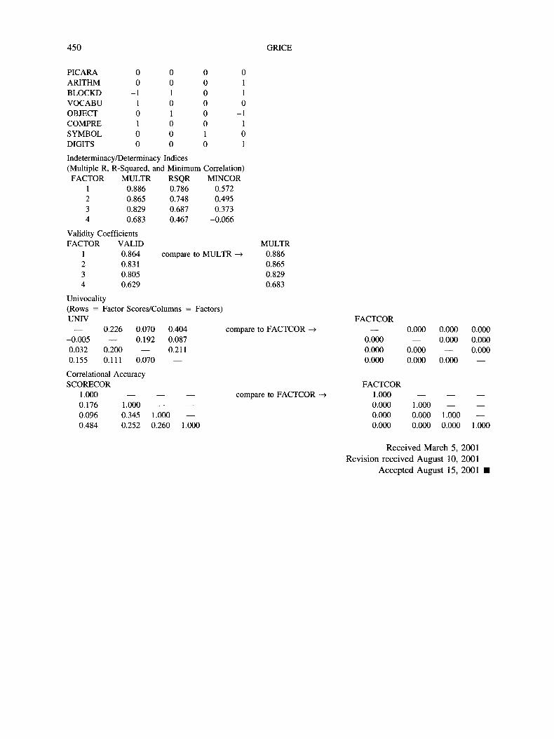
450 GRICE

PICARAARITHMBLOCKDVOCABUOBJECTCOMPRESYMBOLDIGITS

00

-110100

00101000

00000010

0110

-1101

Indeterminacy/Determinacy Indices(Multiple R, R-Squared, and Minimum Correlation)

FACTOR MULTR RSQR MINCOR1 0.886 0.786 0.5722 0.865 0.748 0.4953 0.829 0.687 0.3734 0.683 0.467 -0.066

Validity CoefficientsFACTOR VALID

0.8640.8310.805

compare to MULTR

0.629

Univocality(Rows = Factor Scores/Columns = Factors)UNIV

MULTR0.8860.8650.8290.683

—-0.0050.0320.155

0.226—

0.2000.111

0.0700.192

—0.070

0.4040.0870.211

—

compare to FACTCOR

Correlational AccuracySCORECOR

1.000 — — —0.176 1.000 — —0.096 0.345 1.000 —0.484 0.252 0.260 1.000

compare to FACTCOR ->

FACTCOR

0.0000.0000.000

FACTCOR1.0000.0000.0000.000

0.000 0.000 0.000— 0.000 0.000

0.000 — 0.0000.000 0.000 —

i.ooo — —0.000 1.000 —0.000 0.000 1.000

Received March 5, 2001Revision received August 10, 2001

Accepted August 15, 2001