computer generation of statistical distributions - ftp.arl.mil
TRANSCRIPT
ARMY RESEARCH LABORATORY
Computer Generationof Statistical Distributions
by Richard Saucier
ARL-TR-2168 March 2000
Approved for public release; distribution is unlimited.

ABSTRACT
This report presents a collection of computer–generated statistical distributions which are useful for performingMonte Carlo simulations. The distributions are encapsulated into a C++ class, called ‘‘Random,’’ so that they can beused with any C++ program. The class currently contains 27 continuous distributions, 9 discrete distributions,data–driven distributions, bivariate distributions, and number–theoretic distributions. The class is designed to beflexible and extensible, and this is supported in two ways: (1) a function pointer is provided so that theuser–programmer can specify an arbitrary probability density function, and (2) new distributions can be easily addedby coding them directly into the class. The format of the report is designed to provide the practitioner of MonteCarlo simulations with a handy reference for generating statistical distributions. However, to be self–contained,various techniques for generating distributions are also discussed, as well as procedures for estimating distributionparameters from data. Since most of these distributions rely upon a good underlying uniform distribution of randomnumbers, several candidate generators are presented along with selection criteria and test results. Indeed, it is notedthat one of the more popular generators is probably overused and under what conditions it should be avoided.
ii

ACKNOWLEDGMENTS
The author would like to thank Linda L. C. Moss and Robert Shnidman for correcting a number of errors andsuggesting improvements on an earlier version of this report. The author is especially indebted to Richard S.Sandmeyer for generously sharing his knowledge of this subject area, suggesting generalizations for a number of thedistributions, testing the random number distributions against their analytical values, as well as carefully reviewingthe entire manuscript. Needless to say, any errors that remain are not the fault of the reviewers—nor the author—butrather are to be blamed on the computer.
iii

INTENTIONALLY LEFT BLANK.
iv
TABLE OF CONTENTS
PageACKNOWLEDGMENTS . . . . . . . . . . . . . . . . . . . . . . . . . iiiLIST OF FIGURES . . . . . . . . . . . . . . . . . . . . . . . . . . . viiLIST OF TABLES . . . . . . . . . . . . . . . . . . . . . . . . . . . ix
1. SUMMARY . . . . . . . . . . . . . . . . . . . . . . . . . . . . . 12. INTRODUCTION . . . . . . . . . . . . . . . . . . . . . . . . . . . . 13. METHODS FOR GENERATING RANDOM NUMBER DISTRIBUTIONS . . . . . . . . . 23.1 Inverse Transformation . . . . . . . . . . . . . . . . . . . . . . . . 23.2 Composition . . . . . . . . . . . . . . . . . . . . . . . . . . . 33.3 Convolution . . . . . . . . . . . . . . . . . . . . . . . . . . . . 43.4 Acceptance–Rejection . . . . . . . . . . . . . . . . . . . . . . . . 63.5 Sampling and Data–Driven Techniques . . . . . . . . . . . . . . . . . . . 73.6 Techniques Based on Number Theory. . . . . . . . . . . . . . . . . . . 73.7 MonteCarlo Simulation. . . . . . . . . . . . . . . . . . . . . . . . 73.8 Correlated Bivariate Distributions . . . . . . . . . . . . . . . . . . . . . 93.9 Truncated Distributions . . . . . . . . . . . . . . . . . . . . . . . . 94. PARAMETER ESTIMATION . . . . . . . . . . . . . . . . . . . . . . . . 104.1 Linear Regression (Least–Squares Estimate). . . . . . . . . . . . . . . . . 104.2 Maximum Likelihood Estimation. . . . . . . . . . . . . . . . . . . . . 105. PROBABILITY DISTRIB UTION FUNCTIONS . . . . . . . . . . . . . . . . . . 115.1 Continuous Distributions . . . . . . . . . . . . . . . . . . . . . . . 125.1.1 Arcsine . . . . . . . . . . . . . . . . . . . . . . . . . . . 135.1.2 Beta . . . . . . . . . . . . . . . . . . . . . . . . . . . . 145.1.3 Cauchy (Lorentz) . . . . . . . . . . . . . . . . . . . . . . . . 155.1.4 Chi–Square . . . . . . . . . . . . . . . . . . . . . . . . . . 165.1.5 Cosine . . . . . . . . . . . . . . . . . . . . . . . . . . . 175.1.6 Double Log . . . . . . . . . . . . . . . . . . . . . . . . . . 185.1.7 Erlang . . . . . . . . . . . . . . . . . . . . . . . . . . . 195.1.8 Exponential . . . . . . . . . . . . . . . . . . . . . . . . . . 205.1.9 Extreme Value . . . . . . . . . . . . . . . . . . . . . . . . . 215.1.10 F Ratio . . . . . . . . . . . . . . . . . . . . . . . . . . . 225.1.11 Gamma . . . . . . . . . . . . . . . . . . . . . . . . . . . 235.1.12 Laplace (Double Exponential) . . . . . . . . . . . . . . . . . . . . 255.1.13 Logarithmic . . . . . . . . . . . . . . . . . . . . . . . . . . 265.1.14 Logistic . . . . . . . . . . . . . . . . . . . . . . . . . . . 275.1.15 Lognormal . . . . . . . . . . . . . . . . . . . . . . . . . . 285.1.16 Normal (Gaussian) . . . . . . . . . . . . . . . . . . . . . . . 295.1.17 Parabolic . . . . . . . . . . . . . . . . . . . . . . . . . . . 305.1.18 Pareto . . . . . . . . . . . . . . . . . . . . . . . . . . . . 315.1.19 Pearson’s Type 5 (Inverted Gamma) . . . . . . . . . . . . . . . . . . 325.1.20 Pearson’s Type 6 . . . . . . . . . . . . . . . . . . . . . . . . 335.1.21 Power . . . . . . . . . . . . . . . . . . . . . . . . . . . . 345.1.22 Rayleigh . . . . . . . . . . . . . . . . . . . . . . . . . . . 355.1.23 Student’s t . . . . . . . . . . . . . . . . . . . . . . . . . . 365.1.24 Triangular . . . . . . . . . . . . . . . . . . . . . . . . . . 375.1.25 Uniform . . . . . . . . . . . . . . . . . . . . . . . . . . . 385.1.26 User–Specified . . . . . . . . . . . . . . . . . . . . . . . . . 395.1.27 Weibull . . . . . . . . . . . . . . . . . . . . . . . . . . . 40
v
5.2 DiscreteDistributions . . . . . . . . . . . . . . . . . . . . . . . . . 415.2.1 Bernoulli . . . . . . . . . . . . . . . . . . . . . . . . . . . 425.2.2 Binomial . . . . . . . . . . . . . . . . . . . . . . . . . . . 435.2.3 Geometric . . . . . . . . . . . . . . . . . . . . . . . . . . 445.2.4 Hypergeometric . . . . . . . . . . . . . . . . . . . . . . . . 455.2.5 Multinomial . . . . . . . . . . . . . . . . . . . . . . . . . . 465.2.6 Negative Binomial . . . . . . . . . . . . . . . . . . . . . . . . 475.2.7 Pascal . . . . . . . . . . . . . . . . . . . . . . . . . . . . 485.2.8 Poisson . . . . . . . . . . . . . . . . . . . . . . . . . . . 495.2.9 Uniform Discrete . . . . . . . . . . . . . . . . . . . . . . . . 505.3 Empirical and Data–Driven Distributions . . . . . . . . . . . . . . . . . . 515.3.1 Empirical . . . . . . . . . . . . . . . . . . . . . . . . . . 525.3.2 Empirical Discrete . . . . . . . . . . . . . . . . . . . . . . . . 535.3.3 Sampling With and Without Replacement . . . . . . . . . . . . . . . . 555.3.4 Stochastic Interpolation . . . . . . . . . . . . . . . . . . . . . . 565.4. Bivariate Distributions . . . . . . . . . . . . . . . . . . . . . . . . 585.4.1 Bivariate Normal (Bivariate Gaussian) . . . . . . . . . . . . . . . . . 595.4.2 Bivariate Uniform . . . . . . . . . . . . . . . . . . . . . . . . 605.4.3 Correlated Normal . . . . . . . . . . . . . . . . . . . . . . . . 615.4.4 Correlated Uniform . . . . . . . . . . . . . . . . . . . . . . . 625.4.5 Spherical Uniform . . . . . . . . . . . . . . . . . . . . . . . . 635.4.6 Spherical Uniform in N–Dimensions . . . . . . . . . . . . . . . . . . 645.5 Distributions Generated From Number Theory. . . . . . . . . . . . . . . . . 655.5.1 Tausworthe Random Bit Generator . . . . . . . . . . . . . . . . . . 655.5.2 Maximal Av oidance (Quasi–Random) . . . . . . . . . . . . . . . . . 666. DISCUSSION AND EXAMPLES . . . . . . . . . . . . . . . . . . . . . . 686.1 Making Sense of the Discrete Distributions . . . . . . . . . . . . . . . . . . 686.2 Adding New Distributions . . . . . . . . . . . . . . . . . . . . . . . 696.3 Bootstrap Method as an Application of Sampling. . . . . . . . . . . . . . . . 706.4 MonteCarlo Sampling to Evaluate an Integral . . . . . . . . . . . . . . . . . 726.5 Application of Stochastic Interpolation. . . . . . . . . . . . . . . . . . . 746.6 Combining Maximal Avoidance With Distributions . . . . . . . . . . . . . . . 756.7 Application of Tausworthe Random Bit Vector . . . . . . . . . . . . . . . . . 767. REFERENCES . . . . . . . . . . . . . . . . . . . . . . . . . . . . . 79
APPENDIX A: UNIFORM RANDOM NUMBER GENERATOR . . . . . . . . . . . . 81APPENDIX B: RANDOM CLASS SOURCE CODE . . . . . . . . . . . . . . . . 91GLOSSARY . . . . . . . . . . . . . . . . . . . . . . . . . . . . . 105
vi
LIST OF FIGURES
Figure Page
1. Inverse Transform Method . . . . . . . . . . . . . . . . . . . . . . . . . 22. Probability Density Generated From Uniform Areal Density. . . . . . . . . . . . . . 63. ShapeFactor Probability Density of a Randomly Oriented Cube via Monte Carlo Simulation. . . . 84. CoordinateRotation to Induce Correlations. . . . . . . . . . . . . . . . . . . . 95. ArcsineDensity Function . . . . . . . . . . . . . . . . . . . . . . . . . 136. ArcsineDistribution Function . . . . . . . . . . . . . . . . . . . . . . . . 137. BetaDensity Functions . . . . . . . . . . . . . . . . . . . . . . . . . . 148. BetaDistribution Functions. . . . . . . . . . . . . . . . . . . . . . . . . 149. Cauchy Density Functions . . . . . . . . . . . . . . . . . . . . . . . . . 1510. Cauchy Distribution Functions. . . . . . . . . . . . . . . . . . . . . . . . 1511. Chi–SquareDensity Functions. . . . . . . . . . . . . . . . . . . . . . . . 1612. Chi–SquareDistribution Functions . . . . . . . . . . . . . . . . . . . . . . 1613. CosineDensity Function. . . . . . . . . . . . . . . . . . . . . . . . . . 1714. CosineDistribution Function . . . . . . . . . . . . . . . . . . . . . . . . 1715. DoubleLog Density Function . . . . . . . . . . . . . . . . . . . . . . . . 1816. DoubleLog Distribution Function. . . . . . . . . . . . . . . . . . . . . . . 1817. Erlang Density Functions . . . . . . . . . . . . . . . . . . . . . . . . . 1918. Erlang Distribution Functions . . . . . . . . . . . . . . . . . . . . . . . . 1919. Exponential Density Functions. . . . . . . . . . . . . . . . . . . . . . . . 2020. Exponential Distribution Functions . . . . . . . . . . . . . . . . . . . . . . 2021. ExtremeValue Density Functions. . . . . . . . . . . . . . . . . . . . . . . 2122. ExtremeValue Distribution Functions . . . . . . . . . . . . . . . . . . . . . 2123. F–Ratio Density Function . . . . . . . . . . . . . . . . . . . . . . . . . 2224. F–Ratio Distribution Function . . . . . . . . . . . . . . . . . . . . . . . . 2225. GammaDensity Functions . . . . . . . . . . . . . . . . . . . . . . . . . 2426. GammaDistribution Functions. . . . . . . . . . . . . . . . . . . . . . . . 2427. LaplaceDensity Functions . . . . . . . . . . . . . . . . . . . . . . . . . 2528. LaplaceDistribution Functions. . . . . . . . . . . . . . . . . . . . . . . . 2529. Logarithmic Density Function. . . . . . . . . . . . . . . . . . . . . . . . 2630. Logarithmic Distribution Function . . . . . . . . . . . . . . . . . . . . . . 2631. Logistic Density Functions. . . . . . . . . . . . . . . . . . . . . . . . . 2732. Logistic Distribution Functions. . . . . . . . . . . . . . . . . . . . . . . . 2733. Lognormal Density Functions . . . . . . . . . . . . . . . . . . . . . . . . 2834. Lognormal Distribution Functions. . . . . . . . . . . . . . . . . . . . . . . 2835. Normal Density Function . . . . . . . . . . . . . . . . . . . . . . . . . 2936. Normal Distribution Function . . . . . . . . . . . . . . . . . . . . . . . . 2937. Parabolic Density Function. . . . . . . . . . . . . . . . . . . . . . . . . 3038. Parabolic Distribution Function . . . . . . . . . . . . . . . . . . . . . . . 3039. Pareto Density Functions . . . . . . . . . . . . . . . . . . . . . . . . . 3140. Pareto Distribution Functions . . . . . . . . . . . . . . . . . . . . . . . . 3141. Pearson Type 5 Density Functions. . . . . . . . . . . . . . . . . . . . . . . 3242. Pearson Type 5 Distribution Functions . . . . . . . . . . . . . . . . . . . . . 3243. Pearson Type 6 Density Functions. . . . . . . . . . . . . . . . . . . . . . . 3344. Pearson Type 6 Distribution Functions . . . . . . . . . . . . . . . . . . . . . 3345. Power Density Functions . . . . . . . . . . . . . . . . . . . . . . . . . 3446. Power Distribution Functions . . . . . . . . . . . . . . . . . . . . . . . . 34
vii
47. Rayleigh Density Function . . . . . . . . . . . . . . . . . . . . . . . . . 3548. Rayleigh Distribution Function. . . . . . . . . . . . . . . . . . . . . . . . 3549. Student’s t Density Functions . . . . . . . . . . . . . . . . . . . . . . . . 3650. Student’s t Distribution Functions. . . . . . . . . . . . . . . . . . . . . . . 3651. Triangular Density Functions. . . . . . . . . . . . . . . . . . . . . . . . 3752. Triangular Distribution Functions. . . . . . . . . . . . . . . . . . . . . . . 3753. Uniform Density Function . . . . . . . . . . . . . . . . . . . . . . . . . 3854. Uniform Distribution Function. . . . . . . . . . . . . . . . . . . . . . . . 3855. User–Specified Density Function . . . . . . . . . . . . . . . . . . . . . . . 3956. User–Specified Distribution Function. . . . . . . . . . . . . . . . . . . . . . 3957. Weibull Density Functions . . . . . . . . . . . . . . . . . . . . . . . . . 4058. Weibull Distribution Functions. . . . . . . . . . . . . . . . . . . . . . . . 4059. Binomial Density Function . . . . . . . . . . . . . . . . . . . . . . . . . 4360. Binomial Distribution Function . . . . . . . . . . . . . . . . . . . . . . . 4361. Geometric Density Function . . . . . . . . . . . . . . . . . . . . . . . . 4462. Geometric Distribution Function . . . . . . . . . . . . . . . . . . . . . . . 4463. Hypergeometric Density Function. . . . . . . . . . . . . . . . . . . . . . . 4564. Hypergeometric Distribution Function . . . . . . . . . . . . . . . . . . . . . 4565. Negative Binomial Density Function. . . . . . . . . . . . . . . . . . . . . . 4766. Negative Binomial Distribution Function . . . . . . . . . . . . . . . . . . . . 4767. Pascal Density Function. . . . . . . . . . . . . . . . . . . . . . . . . . 4868. Pascal Distribution Function . . . . . . . . . . . . . . . . . . . . . . . . 4869. Poisson Density Function . . . . . . . . . . . . . . . . . . . . . . . . . 4970. Poisson Distribution Function . . . . . . . . . . . . . . . . . . . . . . . . 4971. Uniform Discrete Density Function . . . . . . . . . . . . . . . . . . . . . . 5072. Uniform Discrete Distribution Function . . . . . . . . . . . . . . . . . . . . . 5073. DiscreteEmpirical Density Function. . . . . . . . . . . . . . . . . . . . . . 5474. DiscreteEmpirical Distribution Function . . . . . . . . . . . . . . . . . . . . 5475. bivariateNormal( 0., 1., 0., 1. ). . . . . . . . . . . . . . . . . . . . . . . . 5976. bivariateNormal( 0., 1., -1., 0.5 ) . . . . . . . . . . . . . . . . . . . . . . . 5977. bivariateUniform( 0., 1., 0., 1. ) . . . . . . . . . . . . . . . . . . . . . . . 6078. bivariateUniform( 0., 1., -1., 0.5 ). . . . . . . . . . . . . . . . . . . . . . . 6079. corrNormal( 0.5, 0., 0., 0., 1. ). . . . . . . . . . . . . . . . . . . . . . . . 6180. corrNormal( -0.75, 0., 1., 0., 0.5 ). . . . . . . . . . . . . . . . . . . . . . . 6181. corrUniform( 0.5, 0., 1., 0., 1. ). . . . . . . . . . . . . . . . . . . . . . . . 6282. corrUniform( -0.75, 0., 1., -1., 0.5 ) . . . . . . . . . . . . . . . . . . . . . . 6283. Uniform Spherical Distribution via spherical(). . . . . . . . . . . . . . . . . . . 6384. Maximal Av oidance Compared to Uniformly Distributed . . . . . . . . . . . . . . . 6685. Semi–Elliptical Density Function . . . . . . . . . . . . . . . . . . . . . . . 6986. Integration as an Area Evaluation via Acceptance–Rejection Algorithm. . . . . . . . . . . 7287. Stochastic Data for Stochastic Interpolation. . . . . . . . . . . . . . . . . . . . 7488. Synthetic Data via Stochastic Interpolation. . . . . . . . . . . . . . . . . . . . 7489. Combining Maximal Avoidance With Bivariate Normal . . . . . . . . . . . . . . . . 7590. Fault Tree for Main Armament of M1A1 Tank . . . . . . . . . . . . . . . . . . . 76
viii
LIST OF TABLES
Table Page
1. Properties for Selecting the Appropriate Continuous Distribution . . . . . . . . . . . . . 12
2. Parameters and Description for Selecting the Appropriate Discrete Distribution . . . . . . . . 41
3. Parameters and Description for Selecting the Appropriate Empirical Distribution . . . . . . . . 51
4. Description and Output for Selecting the Appropriate Bivariate Distribution . . . . . . . . . 58
5. Comparison of Uniform Random and Maximal Avoidance in Monte Carlo Sampling. . . . . . . 73
6. Correlation Coefficient Between Component and Fault Tree Deactivation . . . . . . . . . . 77
7. Ranking of Component Significance to Fault Tree Deactivation . . . . . . . . . . . . . 78
A-1. Capability to Generate Distinct Random Numbers. . . . . . . . . . . . . . . . . . 85
A-2. Uniform Random Number Generator Timings . . . . . . . . . . . . . . . . . . . 86
A-3. Chi–SquareTest Results (at a 0.05 Level of Significance) . . . . . . . . . . . . . . . 87
A-4. Two–Dimensional Chi–Square Test Results (at a 0.05 Level of Significance) . . . . . . . . . 87
A-5. Three–Dimensional Chi–Square Test Results (at a 0.05 Level of Significance) . . . . . . . . . 88
A-6. Runs–Up Test Results (at a 0.05 Level of Significance) . . . . . . . . . . . . . . . . 88
A-7. K–S Test Results (at a 0.05 Level of Significance) . . . . . . . . . . . . . . . . . . 89
ix

INTENTIONALLY LEFT BLANK.
x
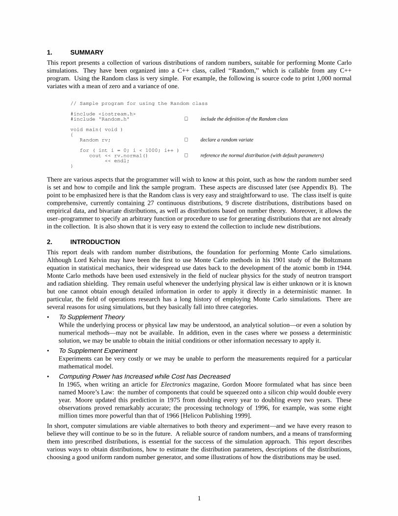
1. SUMMARY
This report presents a collection of various distributions of random numbers, suitable for performing Monte Carlosimulations. They hav e been organized into a C++ class, called ‘‘Random,’’ which is callable from any C++program. Using the Random class is very simple. For example, the following is source code to print 1,000 normalvariates with a mean of zero and a variance of one.
// Sample program for using the Random class
#include <iostream.h>#include "Random.h" ⇐ include the definition of the Random class
void main( void ){
Random rv; ⇐ declarea random variate
for ( int i = 0; i < 1000; i++ )cout << rv.normal() ⇐ reference the normal distribution (with default parameters)
<< endl;}
There are various aspects that the programmer will wish to know at this point, such as how the random number seedis set and how to compile and link the sample program. These aspects are discussed later (see Appendix B). Thepoint to be emphasized here is that the Random class is very easy and straightforward to use. The class itself is quitecomprehensive, currently containing 27 continuous distributions, 9 discrete distributions, distributions based onempirical data, and bivariate distributions, as well as distributions based on number theory. Moreover, it allows theuser–programmer to specify an arbitrary function or procedure to use for generating distributions that are not alreadyin the collection.It is also shown that it is very easy to extend the collection to include new distributions.
2. INTRODUCTION
This report deals with random number distributions, the foundation for performing Monte Carlo simulations.Although Lord Kelvin may have been the first to use Monte Carlo methods in his 1901 study of the Boltzmannequation in statistical mechanics, their widespread use dates back to the development of the atomic bomb in 1944.Monte Carlo methods have been used extensively in the field of nuclear physics for the study of neutron transportand radiation shielding. They remain useful whenever the underlying physical law is either unknown or it is knownbut one cannot obtain enough detailed information in order to apply it directly in a deterministic manner. Inparticular, the field of operations research has a long history of employing Monte Carlo simulations. There areseveral reasons for using simulations, but they basically fall into three categories.
• To Supplement TheoryWhile the underlying process or physical law may be understood, an analytical solution—or even a solution bynumerical methods—may not be available. In addition, even in the cases where we possess a deterministicsolution, we may be unable to obtain the initial conditions or other information necessary to apply it.
• To Supplement ExperimentExperiments can be very costly or we may be unable to perform the measurements required for a particularmathematical model.
• Computing Pow er has Increased while Cost has DecreasedIn 1965, when writing an article for Electronics magazine, Gordon Moore formulated what has since beennamed Moore’s Law: the number of components that could be squeezed onto a silicon chip would double everyyear. Moore updated this prediction in 1975 from doubling every year to doubling every two years. Theseobservations proved remarkably accurate; the processing technology of 1996, for example, was some eightmillion times more powerful than that of 1966 [Helicon Publishing 1999].
In short, computer simulations are viable alternatives to both theory and experiment—and we have every reason tobelieve they will continue to be so in the future. A reliable source of random numbers, and a means of transformingthem into prescribed distributions, is essential for the success of the simulation approach. This report describesvarious ways to obtain distributions, how to estimate the distribution parameters, descriptions of the distributions,choosing a good uniform random number generator, and some illustrations of how the distributions may be used.
1

3. METHODS FOR GENERATING RANDOM NUMBER DISTRIB UTIONS
We wish to generate random numbers,* x, that belong to some domain, x ∈ [xmin, xmax], in such a way that the fre-quency of occurrence, or probability density, will depend upon the value of x in a prescribed functional form f (x).Here, we review sev eral techniques for doing this. We should point out that all of these methods presume that wehave a supply of uniformly distributed random numbers in the half-closed unit inteval [0, 1). These methods areonly concerned with transforming the uniform random variate on the unit interval into another functional form. Thesubject of how to generate the underlying uniform random variates is discussed in Appendix A.
We begin with the inverse transformation technique, as it is probably the easiest to understand and is also the methodmost commonly used. A word on notation: f (x) is used to denote the probability density and F(x) is used to denotethe cumulative distribution function (see the Glossary for a more complete discussion).
3.1 Inverse Transf ormation
If we can invert the cumulative distribution function F(x), then it is a simple matter to generate the probability den-sity function f (x). Thealgorithm for this technique is as follows.
(1) GenerateU ~ U(0, 1).(2) Return X = F−1(U).
It is not difficult to see how this method works, with the aid of Figure 1.
F(x)
x
f (x)
x
Figure1. Inv erse Transform Method.
We take uniformly distributed samples along the y axis between 0 and 1. We see that, where the distribution func-tion F(x) is relatively steep, there will result a high density of points along the x axis (giving a larger value of f (x)),and, on the other hand, where F(x) has a relatively shallow slope, there will result in a corresponding lower densityof points along thex axis (giving a smaller value of f (x)). More formally, if
* Of course, all such numbers generated according to precise and specific algorithms on a computer are not truly random at all but onlyexhibit the appearance of randomness and are therefore best described as ‘‘pseudo-random.’’ Howev er, throughout this report, we use theterm ‘‘random number’’ as merely a shorthand to signify the more correct term of ‘‘pseudo-random number.’’
2
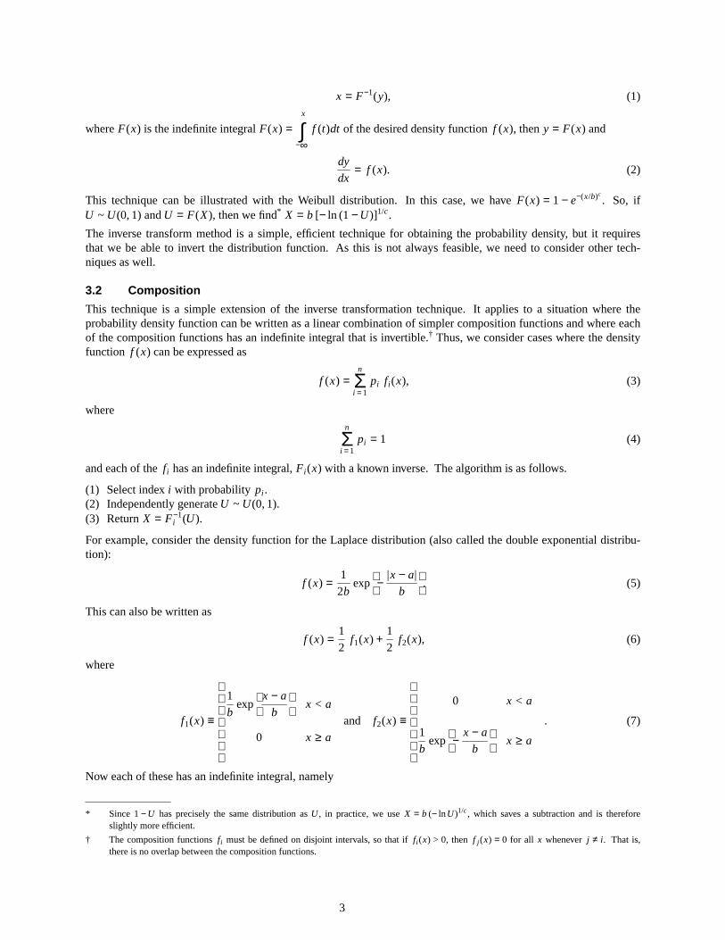
x = F−1(y), (1)
whereF(x) is the indefinite integral F(x) =x
−∞∫ f (t)dt of the desired density functionf (x), theny = F(x) and
dy
dx= f (x). (2)
This technique can be illustrated with the Weibull distribution. In this case, we have F(x) = 1 − e−(x/b)c. So, if
U ~ U(0, 1) andU = F(X), then we find* X = b [− ln (1 −U)]1/c.
The inverse transform method is a simple, efficient technique for obtaining the probability density, but it requiresthat we be able to invert the distribution function. As this is not always feasible, we need to consider other tech-niques as well.
3.2 Composition
This technique is a simple extension of the inverse transformation technique. It applies to a situation where theprobability density function can be written as a linear combination of simpler composition functions and where eachof the composition functions has an indefinite integral that is invertible.† Thus, we consider cases where the densityfunction f (x) can be expressed as
f (x) =n
i =1Σ pi fi (x), (3)
wheren
i =1Σ pi = 1 (4)
and each of thefi has an indefinite integral, Fi (x) with a known inverse. Thealgorithm is as follows.
(1) Select index i with probability pi .(2) Independently generateU ~ U(0, 1).(3) Return X = F−1
i (U).
For example, consider the density function for the Laplace distribution (also called the double exponential distribu-tion):
f (x) =1
2bexp
−
|x − a|
b. (5)
This can also be written as
f (x) =1
2f1(x) +
1
2f2(x), (6)
where
f1(x) ≡
1
bexp
x − a
b
0
x < a
x ≥ a
and f2(x) ≡
0
1
bexp
−
x − a
b
x < a
x ≥ a
. (7)
Now each of these has an indefinite integral, namely
* Since 1 −U has precisely the same distribution as U , in practice, we use X = b (− lnU)1/c, which saves a subtraction and is thereforeslightly more efficient.
† The composition functions fi must be defined on disjoint intervals, so that if fi (x) > 0, then f j (x) = 0 for all x whenever j ≠ i . That is,there is no overlap between the composition functions.
3

F1(x) =
exp
x − a
b
0
x < a
x ≥ a
and F2(x) =
0
1 − exp −
x − a
b
x < a
x ≥ a
, (8)
that is invertible. Since p1 = p2 = 1/2, we can selectU1 ~ U(0, 1) and set
i =
1
2
if U1 ≥ 1/2
if U1 < 1/2. (9)
Independently, weselectU2 ~ U(0, 1) and then, using the inversion technique of section 3.1,
X =
a + b lnU2
a − b lnU2
if i = 1
if i = 2. (10)
3.3 Convolution
If X andY are independent random variables from known density functions fX(x) and fY(y), then we can generatenew distributions by forming various algebraic combinations of X andY. Here, we show how this can be done viasummation, multiplication, and division. We only treat the case when the distributions are independent—in whichcase, the joint probability density function is simply f (x, y) = fX(x) fY(y). First consider summation. The cumula-tive distribution is given by
FX+Y(u) =x+y ≤ u∫ ∫ f (x, y) dx dy (11)
=∞
−∞∫
u−x
y =−∞∫ f (x, y) dy
dx . (12)
The density is obtained by differentiating with respect tou, and this gives us the convolution formula for the sum
fX+Y(u) =∞
−∞∫ f (x, u − x)dx , (13)
where we used Leibniz’s rule (see Glossary) to carry out the differentiation (first on x and then on y). Notice that, ifthe random variables are nonnegative, then the lower limit of integration can be replaced with zero, since fX(x) = 0for all x < 0, and the upper limit can be replaced withu, since fY(u − x) = 0 for x > u.
Let us apply this formula to the sum of two uniform random variables on [0,1]. Wehav e
fX+Y(u) =∞
−∞∫ f (x) f (u − x) dx . (14)
Since f (x) = 1 when 0≤ x ≤ 1, and is zero otherwise, we have
fX+Y(u) =1
0∫ f (u − x) dx =
u
u−1∫ f (t) dt =
u
2 − u
u ≤ 1
1 < u ≤ 2, (15)
and we recognize this as a triangular distribution (see section 5.1.24). As another example, consider the sum of twoindependent exponential random variables with locationa = 0 and scaleb. The density function for the sum is
fX+Y(z) =z
0∫ fX(x) fY(z − x) dx =
z
0∫ 1
be−x/b 1
be−(z−x)/b dx =
1
b2ze−z/b . (16)
Using mathematical induction, it is straightforward to generalize to the case of n independent exponential randomvariates:
4
fX1+...+Xn(x) =
xn−1e−x/b
(n − 1)!bn= gamma (0, b, n), (17)
where we recognized this density as the gamma density for location parameter a = 0, scale parameter b, and shapeparameterc = n (see section 5.1.11).
Thus, the convolution technique for summation applies to a situation where the probability distribution may be writ-ten as a sum of other random variates, each of which can be generated directly. The algorithm is as follows.
(1) Generate Xi ~ F−1i (U) for i = 1, 2, . . . , n.
(2) Set X = X1 + X2 + . . . + Xn.
To pursue this a bit further, we can derive a result that will be useful later. Consider, then, the Erlang distribution; itis a special case of the gamma distribution when the shape parameter c is an integer. From the aforementioned dis-cussion, we see that this is the sum ofc independent exponential random variables (see section 5.1.8), so that
X = − b ln X1 − . . . − b ln Xc = − b ln (X1. . . Xc). (18)
This shows that if we have c IID exponential variates, then the Erlang distribution can be generated via
X = − b lnc
i =1Π Xi . (19)
Random variates may be combined in ways other than summation. Consider the product of X andY. The cumula-tive distribution is
FXY(u) =xy≤ u∫ ∫ f (x, y) dx dy (20)
=∞
−∞∫
u/x
y =−∞∫ f (x, y)dy
dx . (21)
Once again, the density is obtained by differentiating with respect tou:
fXY(u) =∞
−∞∫ f (x, u/x)
1
xdx . (22)
Let us apply this to the product of two uniform densities.We hav e
fXY(u) =∞
−∞∫ f (x) f (u/x)
1
xdx . (23)
On the unit interval, f (x) is zero whenx > 1 and f (u/x) is zero whenx < u. Therefore,
fXY(u) =1
u∫ 1
xdx = − ln u. (24)
This shows that the log distribution can be generated as the product of two IID uniform variates (see section 5.1.13).
Finally, let’s consider the ratio of two variates:
FY/X(u) =y/x ≤ u∫ ∫ f (x, y) dx dy (25)
=∞
−∞∫
ux
y =−∞∫ f (x, y)dy
dx . (26)
Differentiating this to get the density,
5
fY/X(u) =∞
−∞∫ f (x, ux) |x| dx . (27)
As an example, let us apply this to the ratio of two normal variates with mean 0 and variance 1.We hav e
fY/X(u) =∞
−∞∫ f (x) f (ux) |x| dx =
1
2π
∞
−∞∫ e−x2/2e−u2x2/2 |x| dx , (28)
and we find that
fY/X(u) =1
π
∞
0∫ e−(1+u2)x2/2 x dx =
1
π(1 + u2). (29)
This is recognized as a Cauchy distribution (see section 5.1.3).
3.4 Acceptance–Rejection
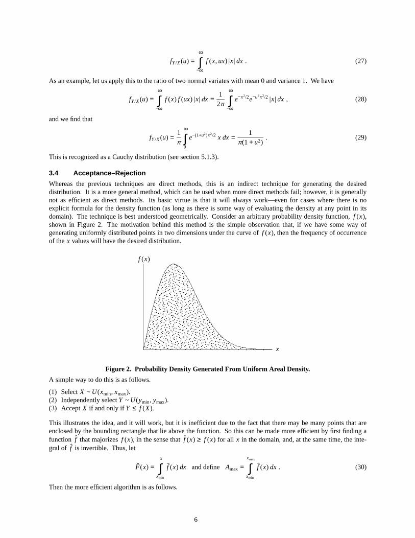
Whereas the previous techniques are direct methods, this is an indirect technique for generating the desireddistribution. It is a more general method, which can be used when more direct methods fail; however, it is generallynot as efficient as direct methods. Its basic virtue is that it will always work—even for cases where there is noexplicit formula for the density function (as long as there is some way of evaluating the density at any point in itsdomain). The technique is best understood geometrically. Consider an arbitrary probability density function, f (x),shown in Figure 2. The motivation behind this method is the simple observation that, if we have some way ofgenerating uniformly distributed points in two dimensions under the curve of f (x), then the frequency of occurrenceof thex values will have the desired distribution.
•
•
•
•
•
•
•
•
•
•
•
•
•
•
•
•
•
•
•
•
•
•
•
• •
•
•
•
•
•
•
•
•
•
•
•
•
•
•
•
•
•
•
•
•
•
•
•
•
•
•
•
•
•
•
•
•
•
•
•
•
•
•
•
•
•
•
•
•
•
•
•
•
•
•
•
•
•
•
•
•
•
•
•
•
•
•
•
•
•
•
•
•
•
•
•
•
•
•
•
•
•
•
•
•
•
•
•
•
•
•
•
•
•
•
•
•
•
•
•
•
•
•
•
•
•
•
••
•
•
•
•
•
•
•
•
•
•
•
•
•
•
•
•
•
•
•
•
•
•
•
•
•
•
•
•
•
•
•
•
•
•
•
•
••
•
•
•
•
•
•
•
•
•
•
•
•
•
•
•
•
•
•
•
•
•
•
•
•
•
•
•
•
•
•
•
•
•
•
•
•
•
•
•
•
•
•
•
•
•
••
•
•
•
•
•
•
•
•
•
•
•
•
•
•
•
•
•
•
•
•
•
•
•
•
•
•
•
•
•
•
•
•
•
•
•
•
•
•
•
•
•
•
•
••
•
•
•
•
•
•
•
•
•
•
•
•
•
•
•
•
•
•
•
•
•
•
•
•
•
•
•
•
•
•
•
•
•
•
•
•
•
•
•
•
•
•
•
•
•
•
•
•
•
•
•
•
•
•
•
•
•
•
•
•
•
•
•
•
•
••
•
•
•
•
•
•
•
•
•
•
•
•
•
•
•
•
•
•
•
•
•
•
•
••
•
•
•
•
•
•
•
•
•
•
•
•
•
•
•
•
•
•
•
•
•
•
•
•
•
•
•
•
•
•
•
•
•
•
•
•
•
•
•
•
•
•
•
•
•
•
•
•
•
•
•
•
•
•
•
•
•
•
•
••
•
•
•
•
•
•
•
•
•
•
•
•
•
•
•
•
•
•
•
•
•
•
•
•
•
•
•
•
•
•
•
•
•
•
•
•
•
•
•
•
•
•
•
•
•
•
•
•
•
•
•
•
•
•
•
•
•
•
•
•
•
•
•
•
•
•
•
•
•
•
•
•
••
•
•
•
•
•
•
•
•
•
••
•
•
•
•
•
•
•
•
•
•
•
•
•
•
•
•
•
•
•
•
•
•
•
•
•
•
•
•
•
•
•
•
•
•
•
•
•
•
•
•
•
•
•
•
•
•
•
•
•
•
•
•
•
•
•
•
•
•
•
•
•
•
•
•
•
•
•
•
•
•
•
•
•
•
•
•
•
•
•
•
•
•
•
•
•
•
•
•
•
•
•
•
•
•
•
•
•
•
•
•
•
•
•
•
•
•
•
•
•
•
•
•
•
•
•
•
•
•
•
•
•
•
•
•
•
•
•
•
•
•
•
•
•
•
•
•
•
•
•
••
•
•
•
•
•
•
•
•
•
•
•
•
•
•
•
•
•
•
•
•
•
•
•
•
•
•
•
•
•
•
•
•
•
•
•
•
•
•
•
•
•
•
•
•
•
•
• •
•
•
•
•
•
•
•
•
•
•
•
•
•
•
•
•
•
•
•
•
•
•
•
•
•
•
•
•
•
•
•
•
•
•
•
•
•
•
•
•
•
•
•
•
•
•
•
•
•
•
•
•
•
•
•
•
f (x)
x
Figure2. Probability Density Generated From Uniform Ar eal Density.
A simple way to do this is as follows.
(1) Select X ~ U(xmin, xmax).(2) Independently selectY ~ U(ymin, ymax).(3) Accept X if and only ifY ≤ f (X).
This illustrates the idea, and it will work, but it is inefficient due to the fact that there may be many points that areenclosed by the bounding rectangle that lie above the function. So this can be made more efficient by first finding afunction f̂ that majorizes f (x), in the sense that f̂ (x) ≥ f (x) for all x in the domain, and, at the same time, the inte-gral of f̂ is invertible. Thus, let
F̂(x) =x
xmin
∫ f̂ (x) dx and define Amax =xmax
xmin
∫ f̂ (x) dx . (30)
Then the more efficient algorithm is as follows.
6
(1) Select A ~ U(0, Amax).
(2) Compute X = F̂−1
(A).(3) Independently selectY ~ U(0, f̂ (X)).(4) Accept X if and only ifY ≤ f (X).
The acceptance-rejection technique can be illustrated with the following example. Let f (x) = 10, 296 x5(1 − x)7. Itwould be very difficult to use the inverse transform method upon this function, since it would involve finding theroots of a 13th degree polynomial. From calculus, we find that f (x) has a maximum value of 2.97187 at x = 5/12.Therefore, the function f̂ (x) = 2. 97187 majorizes f (x). So, with Amax = 2. 97187, F(x) = 2. 97187 x, andymax = 2. 97187, the algorithm is as follows.
(1) Select A ~ U(0, 2. 97187).(2) Compute X = A / 2. 97187.(3) Independently selectY ~ U(0, 2. 97187).(4) Accept X if and only ifY ≤ f (X).
3.5 Sampling and Data–Driven T echniques
One very simple technique for generating distributions is to sample from a given set of data. The simplest techniqueis to sample with replacement, which effectively treats the data points as independent. The generated distribution isa synthetic data set in which some fraction of the original data is duplicated. The bootstrap method (Diaconis andEfron 1983) uses this technique to generate bounds on statistical measures for which analytical formulas are notknown. As such, it can be considered as a Monte Carlo simulation (see section 3.7) We can also sample withoutreplacement, which effectively treats the data as dependent. A simple way of doing this is to first perform a randomshuffle of the data and then to return the data in sequential order. Both of these sampling techniques are discussed insection 5.3.3.
Sampling empirical data works well as far as it goes. It is simple and fast, but it is unable to go beyond the datapoints to generate new points. A classic example that illustrates its limitation is the distribution of darts thrown at adart board. If a bull’s eye is not contained in the data, it will never be generated with sampling. The standard way tohandle this is to first fit a known density function to the data and then draw samples from it. The question arises asto whether it is possible to make use of the data directly without having to fit a distribution beforehand, and yetreturn new values. Fortunately, there is a technique for doing this. It goes by the name of ‘‘data-based simulation’’or, the name preferred here,‘‘stochastic interpolation.’’ This is a more sophisticated technique that will generate newdata points, which have the same statistical properties as the original data at a local level, but without having to paythe price of fitting a distribution beforehand. The underlying theory is discussed in (Taylor and Thompson 1986;Thompson 1989; Bodt and Taylor 1982) and is presented in section 5.3.4.
3.6 Techniques Based on Number Theor y
Number theory has been used to generate random bits of 0 and 1 in a very efficient manner and also to producequasi-random sequences. The latter are sequences of points that take on the appearance of randomness while, at thesame time, possessing other desirable properties.Tw o techniques are included in this report.
1. Primitive Polynomials Modulo TwoThese are useful for generating random bits of 1’s and 0’s that cycle through all possible combinations (exclud-ing all zeros) before repeating.This is discussed in section 5.5.1.
2. Prime Number TheoryThis has been exploited to produce sequences of quasi-random numbers that are self-avoiding. This is dis-cussed in section 5.5.2.
3.7 Monte Carlo Sim ulation
Monte Carlo simulation is a very powerful technique that can be used when the underlying probability density isunknown, or does not come from a known function, but we have a model or method that can be used to simulate thedesired distribution. Unlike the other techniques discussed so far, there is not a direct implementation of this methodin section 5, due to its generality. Instead, we use this opportunity to illustrate this technique. For this purpose, weuse an example that occurs in fragment penetration of plate targets.
7
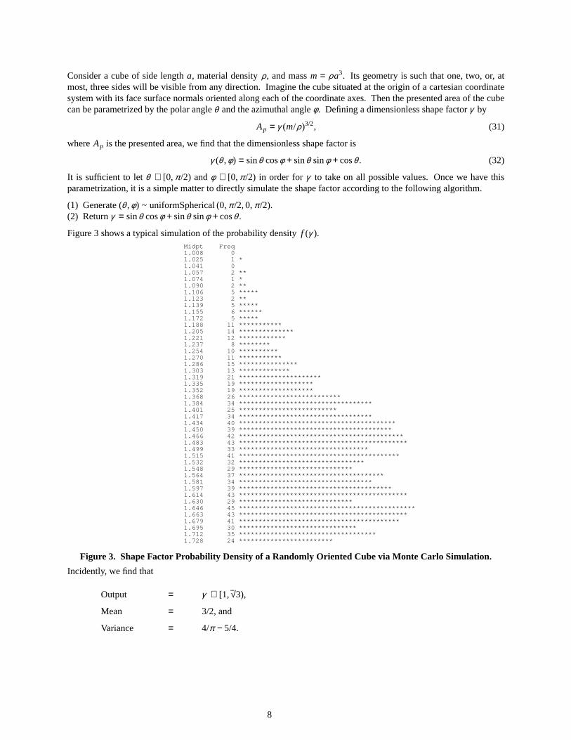
Consider a cube of side length a, material density ρ, and mass m = ρa3. Its geometry is such that one, two, or, atmost, three sides will be visible from any direction. Imagine the cube situated at the origin of a cartesian coordinatesystem with its face surface normals oriented along each of the coordinate axes. Then the presented area of the cubecan be parametrized by the polar angleθ and the azimuthal angleφ. Defining a dimensionless shape factorγ by
Ap = γ (m/ρ)3/2, (31)
whereAp is the presented area, we find that the dimensionless shape factor is
γ (θ ,φ) = sinθ cosφ + sinθ sinφ + cosθ . (32)
It is sufficient to let θ ∈ [0, π/2) and φ ∈ [0, π/2) in order for γ to take on all possible values. Once we have thisparametrization, it is a simple matter to directly simulate the shape factor according to the following algorithm.
(1) Generate (θ ,φ) ~ uniformSpherical (0, π/2, 0, π/2).(2) Return γ = sinθ cosφ + sinθ sinφ + cosθ .
Figure 3 shows a typical simulation of the probability densityf (γ ).Mi dpt Fr eq1. 008 01. 025 1 *1. 041 01. 057 2 **1. 074 1 *1. 090 2 **1. 106 5 *****1. 123 2 **1. 139 5 *****1. 155 6 ******1. 172 5 *****1. 188 11 ***********1. 205 14 **************1. 221 12 ************1. 237 8 ********1. 254 10 **********1. 270 11 ***********1. 286 15 ***************1. 303 13 *************1. 319 21 *********************1. 335 19 *******************1. 352 19 *******************1. 368 26 **************************1. 384 34 **********************************1. 401 25 *************************1. 417 34 **********************************1. 434 40 ****************************************1. 450 39 ***************************************1. 466 42 ******************************************1. 483 43 *******************************************1. 499 33 *********************************1. 515 41 *****************************************1. 532 32 ********************************1. 548 29 *****************************1. 564 37 *************************************1. 581 34 **********************************1. 597 39 ***************************************1. 614 43 *******************************************1. 630 29 *****************************1. 646 45 *********************************************1. 663 43 *******************************************1. 679 41 *****************************************1. 695 30 ******************************1. 712 35 ***********************************1. 728 24 ************************
Figure3. Shape Factor Probability Density of a Randomly Oriented Cube via Monte Carlo Simulation.
Incidently, wefind that
Output = γ ∈ [1, √ 3),
Mean = 3/2, and
Variance = 4/π − 5/4.
8
3.8 Correlated Biv ariate Distrib utions
If we need to generate bivariate distributions and the variates are independent, then we simply generate the distribu-tion for each dimension separately. Howev er, there may be known correlations between the variates. Here, we showhow to generate correlated bivariate distributions.
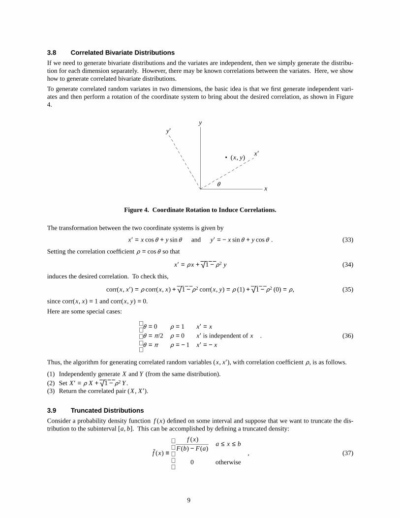
To generate correlated random variates in two dimensions, the basic idea is that we first generate independent vari-ates and then perform a rotation of the coordinate system to bring about the desired correlation, as shown in Figure4.
• (x, y)
x
y
x′
y′
θ
Figure4. Coordinate Rotation to Induce Correlations.
The transformation between the two coordinate systems is given by
x′ = x cosθ + y sinθ and y′ = − x sinθ + y cosθ . (33)
Setting the correlation coefficient ρ = cosθ so that
x′ = ρ x + √ 1 − ρ2 y (34)
induces the desired correlation.To check this,
corr(x, x′) = ρ corr(x, x) + √ 1 − ρ2 corr(x, y) = ρ (1) + √ 1 − ρ2 (0) = ρ, (35)
since corr(x, x) = 1 and corr(x, y) = 0.
Here are some special cases:
θ = 0
θ = π/2
θ = π
ρ = 1
ρ = 0
ρ = − 1
x′ = x
x′ is independent ofx
x′ = − x
. (36)
Thus, the algorithm for generating correlated random variables (x, x′), with correlation coefficient ρ, is as follows.
(1) Independently generateX andY (from the same distribution).
(2) Set X′ = ρ X + √ 1 − ρ2 Y.(3) Return the correlated pair (X, X′).
3.9 Truncated Distrib utions
Consider a probability density function f (x) defined on some interval and suppose that we want to truncate the dis-tribution to the subinterval [a, b]. This can be accomplished by defining a truncated density:
f̃ (x) ≡
f (x)
F(b) − F(a)
0
a ≤ x ≤ b
otherwise
, (37)
9
which has corresponding truncated distribution
F̃(x) ≡
0F(x) − F(a)
F(b) − F(a)1
x < a
a ≤ x ≤ b
x > b
. (38)
An algorithm for generating random variates having distribution functionF̃ is as follows.
(1) GenerateU ~ U(0, 1).(2) Set Y = F(a) + [F(b) − F(a)] U .(3) Return X = F−1(Y).
This method works well with the inverse-transform method. However, if an explicit formula for the function F isnot available for forming the truncated distribution given in equation (38), or if we do not have an explicit formulafor F−1, then a less efficient but nevertheless correct method of producing the truncated distribution is the followingalgorithm.
(1) GenerateacandidateX from the distribution F .(2) If a ≤ X ≤ b, then acceptX; otherwise, go back to step 1.
This algorithm essentially throws away variates that lie outside the domain of interest.
4. PARAMETER ESTIMATION
The distributions presented in section 5 have parameters that are either known or have to be estimated from data. Inthe case of continuous distributions, these may include the location parameter, a; the scale parameter, b; and/or theshape parameter, c. In some cases, we need to specify the range of the random variate,xmin andxmax. In the case ofthe discrete distributions, we may need to specify the probability of occurrence, p, and the number of trials, n. Here,we show how these parameters may be estimated from data and present two techniques for doing this.
4.1 Linear Regression (Least–Squares Estimate)
Sometimes, it is possible to linearize the cumulative distribution function by transformation and then to perform amultiple regression to determine the values of the parameters. It can best be explained with an example. Considerthe Weibull distribution with locationa = 0:
F(x) = 1 − exp[−(x/b)c] . (39)
We first sort the dataxi in accending order:
x1 ≤ x2 ≤ x3 ≤ . . . ≤ xN . (40)
The corresponding cumulative probability is F(xi ) = Fi = i /N. Rearranging eq. (39) so that the parameters appearlinearly, wehav e
ln[− ln(1 − Fi )] = c ln xi − c ln b . (41)
This shows that if we regress the left-hand side of this equation against the logarithms of the data, then we shouldget a straight line.* The least-squares fit will give the parameter c as the slope of the line and the quantity −c ln b asthe intercept, from which we easily determineb andc.
4.2 Maximum Likelihood Estimation
In this method, we assume that the given data came from some underlying distribution that contains a parameter βwhose value is unknown. The probability of getting the observed data with the given distribution is the product ofthe individual densities:
L(β ) = fβ (X1) fβ (X2) . . . fβ (XN) . (42)
* We should note that linearizing the cumulative distribution will also transform the error term. Normally distributed errors will be trans-formed into something other than a normal distribution. However, the error distribution is rarely known, and assuming it is Gaussian tobegin with is usually no more than an act of faith. See the chapter ‘‘Modeling of Data’’ in Press et al. (1992) for a discussion of this point.
10
The value of β that maximizes L(β ) is the best estimate in the sense of maximizing the probability. In practice, it iseasier to deal with the logarithm of the likelihood function (which has the same location as the likelihood functionitself).
As an example, consider the lognormal distribution. Thedensity function is
fµ,σ 2(x) =
1
√ 2π σ xexp
−
(ln x − µ)2
2σ 2
0
x > 0
otherwise
. (43)
The log-likelihood function is
ln L(µ,σ 2) = lnN
i =1Π fµ,σ 2(xi ) =
N
i =1Σ ln fµ,σ 2(xi ) (44)
and, in this case,
ln L(µ,σ 2) =N
i =1Σ
ln(√ 2πσ 2xi ) +
(ln xi − µ)2
2σ 2
. (45)
This is a maximuum when both
∂ ln L(µ,σ 2)
∂µ= 0 and
∂ ln L(µ,σ 2)
∂σ 2= 0 (46)
and we find
µ =1
N
N
i =1Σ ln xi and σ 2 =
1
N
N
i =1Σ (ln xi − µ)2 . (47)
Thus, maximum likelihood parameter estimation leads to a very simple procedure in this case. First, take the loga-rithms of all the data points.Then,µ is the sample mean, andσ 2 is the sample variance.
5. PROBABILITY DISTRIB UTION FUNCTIONS
In this section, we present the random number distributions in a form intended to be most useful to the actual prac-tioner of Monte Carlo simulations.The distributions are divided into fivesubsections as follows.
Continuous DistributionsThere are 27 continuous distributions. For the most part, they make use of three parameters: a location parame-ter, a; a scale parameter, b; and a shape parameter, c. There are a few exceptions to this notation. In the case ofthe normal distribution, for instance, it is customary to use µ for the location parameter and σ for the scaleparameter. In the case of the beta distribution, there are two shape parameters and these are denoted by v andw.Also, in some cases, it is more convenient for the user to select the interval via xmin and xmax than the locationand scale. The location parameter merely shifts the position of the distribution on the x-axis without affectingthe shape, and the scale parameter merely compresses or expands the distribution, also without affecting theshape. The shape parameter may have a small effect on the overall appearance, such as in the Weibull distribu-tion, or it may have a profound effect, as in the beta distribution.
Discrete DistributionsThere are nine discrete distributions. For the most part, they make use of the probability of an event, p, and thenumber of trials,n.
Empir ical and Data-Driven DistributionsThere are four empirical distributions.
Bivar iate Distr ibutionsThere are fivebivariate distributions.
Distr ibutions Generated from Number TheoryThere are two number-theoretic distributions.
11

5.1 Continuous Distrib utions
To aid in selecting an appropriate distribution, we have summarized some characteristics of the continuous distribu-tions in Table 1. The subsections that follow describe each distribution in more detail.
Table 1. Properties for Selecting the Appropriate Continuous Distribution
Distribution Name Parameters Symmetric About the Mode
Arcsin xmin andxmax yes
Beta xmin, xmax, and shapev andw only whenv andw are equal
Cauchy (Lorentz) location a and scaleb yes
Chi–Square shape v (degrees of freedom) no
Cosine xmin andxmax yes
Double Log xmin andxmax yes
Erlang scale b and shapec no
Exponential location a and scaleb no
Extreme Value location a and scaleb no
F Ratio shape v andw (degrees of freedom) no
Gamma location a, scaleb, and shapec no
Laplace (Double Exponential) locationa and scaleb yes
Logarithmic xmin andxmax no
Logistic location a and scaleb yes
Lognormal location a, scaleµ, and shapeσ no
Normal (Gaussian) locationµ and scaleσ yes
Parabolic xmin andxmax yes
Pareto shape c no
Pearson’s Type 5 (Inverted Gamma) scaleb and shapec no
Pearson’s Type 6 scaleb and shapev andw no
Power shape c no
Rayleigh location a and scaleb no
Student’s t shapeν (degrees of freedom) yes
Triangular xmin, xmax, and shapec only whenc = (xmin + xmax)/2
Uniform xmin andxmax yes
User–Specified xmin, xmax andymin, ymax depends upon the function
Weibull location a, scaleb, and shapec no
12
5.1.1 Arcsine
Density Function: f (x) =
1
π√ x(1 − x)
0
0 ≤ x ≤ 1
otherwise
Distribution Function: F(x) =
02
πsin−1(√ x)
1
x < 0
0 ≤ x ≤ 1
x > 1
Input: xmin, minimum value of random variable;xmax, maximum value of random variable
Output: x ∈ [xmin, xmax)
Mode: xmin andxmax
Median: (xmin + xmax)/2
Mean: (xmin + xmax)/2
Variance: (xmax − xmin)2/8
Regression Equation: sin2(Fiπ/2) = xi /(xmax − xmin) − xmin/(xmax − xmin),where thexi are arranged in ascending order, Fi = i /N, and i = 1, 2, . . . , N
Algorithm: (1) GenerateU ~ U(0, 1)(2) Return X = xmin + (xmax − xmin) sin2(Uπ/2)
Source Code: double arcsine( double xMin, double xMax ){
assert( xMin < xMax );
double q = sin( M_PI_2 * uniform( 0., 1. ) );return xMin + ( xMax - xMin ) * q * q;
}
Notes: This is a special case of thebetadistribution (whenv = w = 1/2).
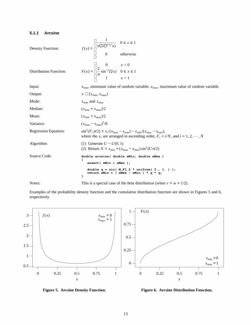
Examples of the probability density function and the cumulative distribution function are shown in Figures 5 and 6,respectively.
0.5
1
1.5
2
2.5
3 xmin = 0xmax = 1
0 0.25 0.5 0.75 1x
f (x)
Figure5. Arcsine Density Function.
xmin =0xmax=1
0 0.25 0.5 0.75 1
0
0.25
0.5
0.75
1
x
F(x)
Figure6. Arcsine Distribution Function.
13
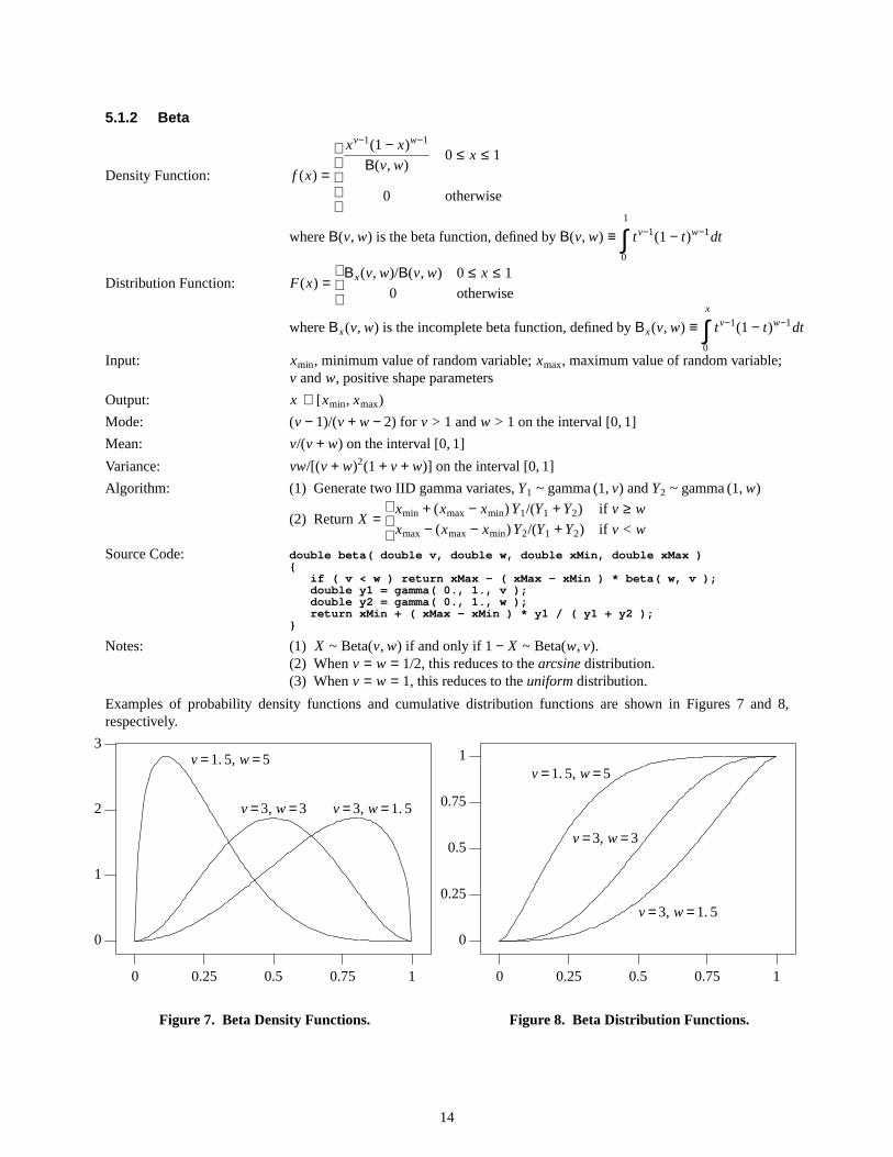
5.1.2 Beta
Density Function: f (x) =
xv−1(1 − x)w−1
Β(v, w)
0
0 ≤ x ≤ 1
otherwise
whereΒ(v, w) is the beta function, defined byΒ(v, w) ≡1
0∫ tv−1(1 − t)w−1dt
Distribution Function: F(x) =
Βx(v, w)/Β(v, w)
0
0 ≤ x ≤ 1
otherwise
whereΒx(v, w) is the incomplete beta function, defined byΒx(v, w) ≡x
0∫ tv−1(1 − t)w−1dt
Input: xmin, minimum value of random variable;xmax, maximum value of random variable;v andw, positive shape parameters
Output: x ∈ [xmin, xmax)
Mode: (v − 1)/(v + w − 2) for v > 1 andw > 1 on the interval [0,1]
Mean: v/(v + w) on the interval [0,1]
Variance: vw/[(v + w)2(1 + v + w)] on the interval [0,1]
Algorithm: (1) Generate two IID gamma variates,Y1 ~ gamma (1, v) andY2 ~ gamma (1, w)
(2) Return X =
xmin + (xmax − xmin) Y1/(Y1 + Y2)
xmax − (xmax − xmin) Y2/(Y1 + Y2)
if v ≥ w
if v < w
Source Code: double beta( double v, double w, double xMin, double xMax ){
if ( v < w ) return xMax - ( xMax - xMin ) * beta( w, v );double y1 = gamma( 0., 1., v );double y2 = gamma( 0., 1., w );return xMin + ( xMax - xMin ) * y1 / ( y1 + y2 );
}
Notes: (1) X ~ Beta(v, w) if and only if 1− X ~ Beta(w, v).(2) When v = w = 1/2, this reduces to thearcsinedistribution.(3) When v = w = 1, this reduces to theuniformdistribution.
Examples of probability density functions and cumulative distribution functions are shown in Figures 7 and 8,respectively.
0
1
2
3v =1. 5, w =5
v =3, w =3 v =3, w =1. 5
0 0.25 0.5 0.75 1
Figure7. Beta Density Functions.
v =1. 5, w =5
v =3, w =3
v =3, w =1. 5
0 0.25 0.5 0.75 1
0
0.25
0.5
0.75
1
Figure8. Beta Distribution Functions.
14
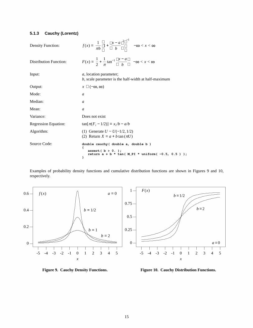
5.1.3 Cauchy (Lorentz)
Density Function: f (x) =1
πb
1 +
x − a
b
2
−1
−∞ < x < ∞
Distribution Function: F(x) =1
2+
1
πtan−1
x − a
b
−∞ < x < ∞
Input: a, location parameter;b, scale parameter is the half-width at half-maximum
Output: x ∈ (−∞,∞)
Mode: a
Median: a
Mean: a
Variance: Does not exist
Regression Equation: tan[π(Fi − 1/2)] = xi /b − a/b
Algorithm: (1) GenerateU ~ U(−1/2, 1/2)(2) Return X = a + b tan (πU)
Source Code: double cauchy( double a, double b ){
assert( b > 0. );return a + b * tan( M_PI * uniform( -0.5, 0.5 ) );
}
Examples of probability density functions and cumulative distribution functions are shown in Figures 9 and 10,respectively.
0
0.2
0.4
0.6
b = 1/2
b = 1
b = 2
-5 -4 -3 -2 -1 0 1 2 3 4 5x
f (x) a = 0
Figure9. Cauchy Density Functions.
-5 -4 -3 -2 -1 0 1 2 3 4 5
0
0.25
0.5
0.75
1
a =0
b=1/2
b=2
F(x)
x
Figure10. Cauchy Distrib ution Functions.
15

5.1.4 Chi-Square
Density Function: f (x) =
xν /2−1e−x/2
2ν /2Γ(ν /2)
0
if x > 0
otherwise
whereΓ(z) is the gamma function, defined byΓ(z) ≡∞
0∫ t z−1e−t dt
Distribution Function:
F(x) =1
2ν /2Γ(ν /2)
x
0∫ tν /2−1e−t/2 dt
0
if x > 0
otherwise
Input: Shapeparameterν ≥ 1 is the number of degrees of freedom
Output: x ∈ (0,∞)
Mode: ν − 2 forν ≥ 2
Mean: ν
Variance: 2ν
Algorithm: ReturnX ~ gamma (0, 2,ν /2)
Source Code: double chiSquare( int df ){
assert( df >= 1 );return gamma( 0., 2., 0.5 * double( df ) );
}
Notes: (1) Thechi-square distribution withν degrees of freedom is equal to the gammadistribution with a scale parameter of 2 and a shape parameter ofν /2.
(2) Let Xi ~ N(0, 1) be IID normal variates fori = 1,. . . ,ν . ThenX2 =ν
i =1Σ X2
i
is a χ 2 distribution withν degrees of freedom.
Examples of probability density functions and cumulative distribution functions are shown in Figures 11 and 12,respectively.
ν =1
ν =2
ν =3
f (x)
0 2 4 6 8 10
0
0.25
0.5
0.75
Figure11. Chi-SquareDensity Functions.
F(x)
ν =1
ν =2
ν =3
0 2 4 6 8 10
0
0.25
0.5
0.75
1
Figure12. Chi-SquareDistrib ution Functions.
16
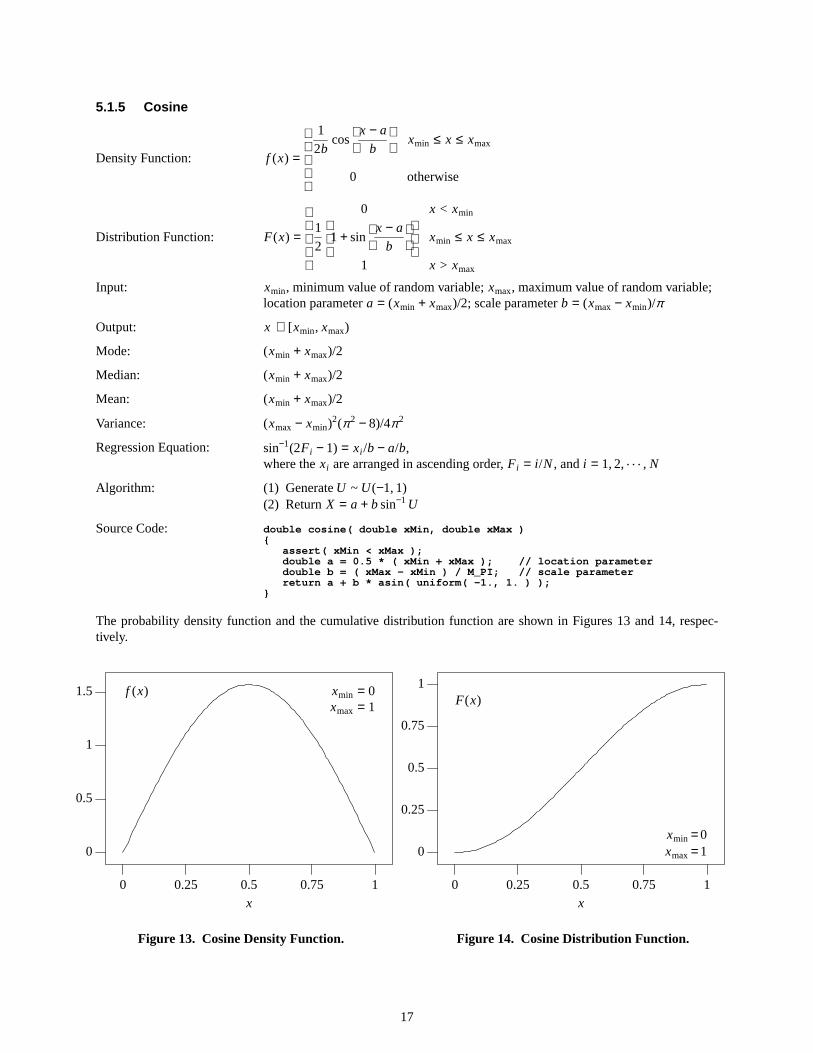
5.1.5 Cosine
Density Function: f (x) =
1
2bcos
x − a
b
0
xmin ≤ x ≤ xmax
otherwise
Distribution Function: F(x) =
0
1
2
1 + sin
x − a
b
1
x < xmin
xmin ≤ x ≤ xmax
x > xmax
Input: xmin, minimum value of random variable;xmax, maximum value of random variable;location parametera = (xmin + xmax)/2; scale parameterb = (xmax − xmin)/π
Output: x ∈ [xmin, xmax)
Mode: (xmin + xmax)/2
Median: (xmin + xmax)/2
Mean: (xmin + xmax)/2
Variance: (xmax − xmin)2(π2 − 8)/4π2
Regression Equation: sin−1(2Fi − 1) = xi /b − a/b,where thexi are arranged in ascending order, Fi = i /N, and i = 1, 2, . . . , N
Algorithm: (1) GenerateU ~ U(−1, 1)(2) Return X = a + bsin−1 U
Source Code: double cosine( double xMin, double xMax ){
assert( xMin < xMax );double a = 0.5 * ( xMin + xMax ); // location parameterdouble b = ( xMax - xMin ) / M_PI; // scale parameterreturn a + b * asin( uniform( -1., 1. ) );
}
The probability density function and the cumulative distribution function are shown in Figures 13 and 14, respec-tively.
0
0.5
1
1.5 xmin = 0xmax = 1
0 0.25 0.5 0.75 1x
f (x)
Figure13. CosineDensity Function.
xmin =0xmax=1
0 0.25 0.5 0.75 1
0
0.25
0.5
0.75
1
x
F(x)
Figure14. CosineDistrib ution Function.
17
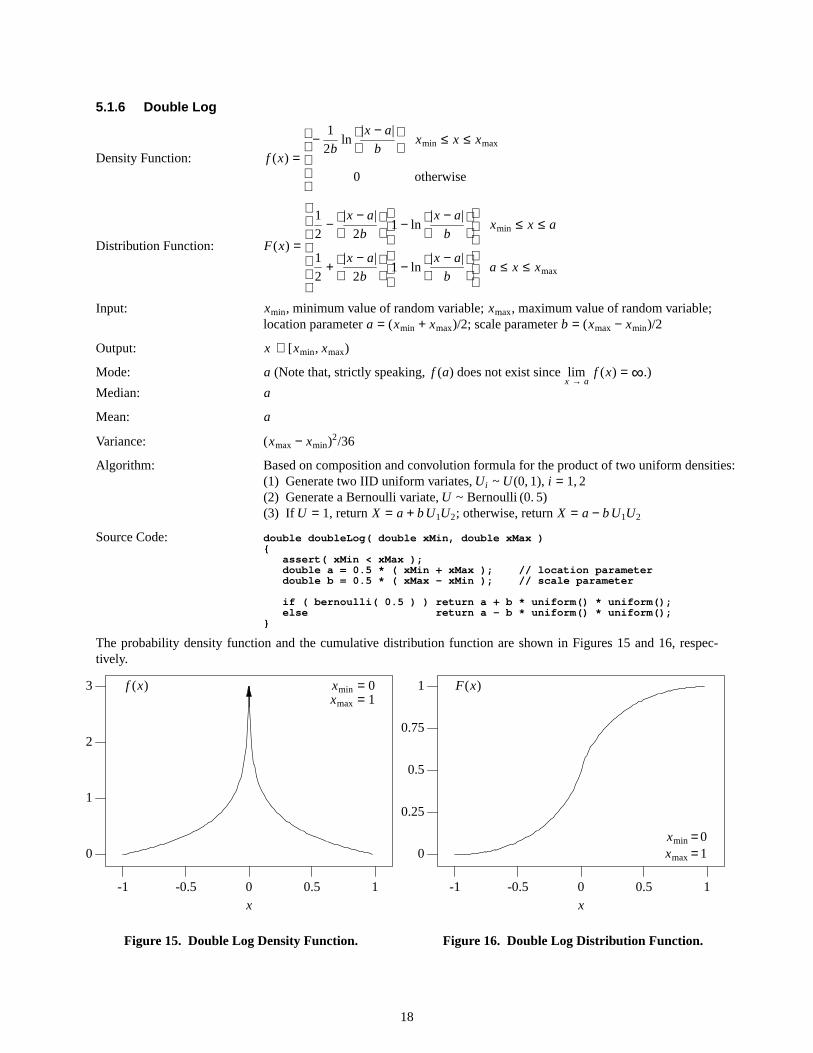
5.1.6 Double Log
Density Function: f (x) =
−1
2bln
|x − a|
b
0
xmin ≤ x ≤ xmax
otherwise
Distribution Function: F(x) =
1
2−
|x − a|
2b
1 − ln
|x − a|
b
1
2+
|x − a|
2b
1 − ln
|x − a|
b
xmin ≤ x ≤ a
a ≤ x ≤ xmax
Input: xmin, minimum value of random variable;xmax, maximum value of random variable;location parametera = (xmin + xmax)/2; scale parameterb = (xmax − xmin)/2
Output: x ∈ [xmin, xmax)
Mode: a (Note that, strictly speaking,f (a) does not exist sincex → alim f (x) = ∞.)
Median: a
Mean: a
Variance: (xmax − xmin)2/36
Algorithm: Based on composition and convolution formula for the product of two uniform densities:(1) Generate two IID uniform variates,Ui ~ U(0, 1), i = 1, 2(2) GenerateaBernoulli variate,U ~ Bernoulli (0. 5)(3) If U = 1, returnX = a + bU1U2; otherwise, returnX = a − bU1U2
Source Code: double doubleLog( double xMin, double xMax ){
assert( xMin < xMax );double a = 0.5 * ( xMin + xMax ); // location parameterdouble b = 0.5 * ( xMax - xMin ); // scale parameter
if ( bernoulli( 0.5 ) ) return a + b * uniform() * uniform();el se r et ur n a - b * uniform() * uniform();
}
The probability density function and the cumulative distribution function are shown in Figures 15 and 16, respec-tively.
0
1
2
3 xmin = 0xmax = 1
-1 -0.5 0 0.5 1x
f (x)
Figure15. DoubleLog Density Function.
xmin =0xmax=1
-1 -0.5 0 0.5 1
0
0.25
0.5
0.75
1
x
F(x)
Figure16. DoubleLog Distribution Function.
18

5.1.7 Erlang
Density Function: f (x) =
(x/b)c−1e−x/b
b(c − 1)!
0
x ≥ 0
otherwise
Distribution Function: F(x) =
1 − e−x/bc−1
i =0Σ (x/b)i
i !
0
x ≥ 0
otherwise
Input: Scaleparameterb > 0; shape parameterc, apositive integer
Output: x ∈ [0,∞)
Mode: b(c − 1)
Mean: bc
Variance: b2c
Algorithm: This algorithm is based on the convolution formula.(1) Generate c IID uniform variates,Ui ~ U(0, 1)
(2) Return X = − bc
i =1Σ lnUi = − b ln
c
i =1Π Ui
Source Code: double erlang( double b, int c ){
assert( b > 0. && c >= 1 );
double prod = 1.0;for ( int i = 0; i < c; i++ ) prod *= uniform( 0., 1. );return -b * log( prod );
}
Notes: The Erlang random variate is the sum of c exponentially-distributed random variates,each with meanb. It reduces to the exponential distribution whenc = 1.
Examples of probability density functions and cumulative distribution functions are shown in Figures 17 and 18,respectively.
0 1 2 3 4 5 6
0
0.25
0.5
0.75
1
c =1
c =2
c =3
b=1
x
f (x)
Figure17. Er lang Density Functions.
x
F(x)
0
0.25
0.5
0.75
1
0 1 2 3 4 5 6
c =1c =2
c =3
b=1
Figure18. Er lang Distrib ution Functions.
19
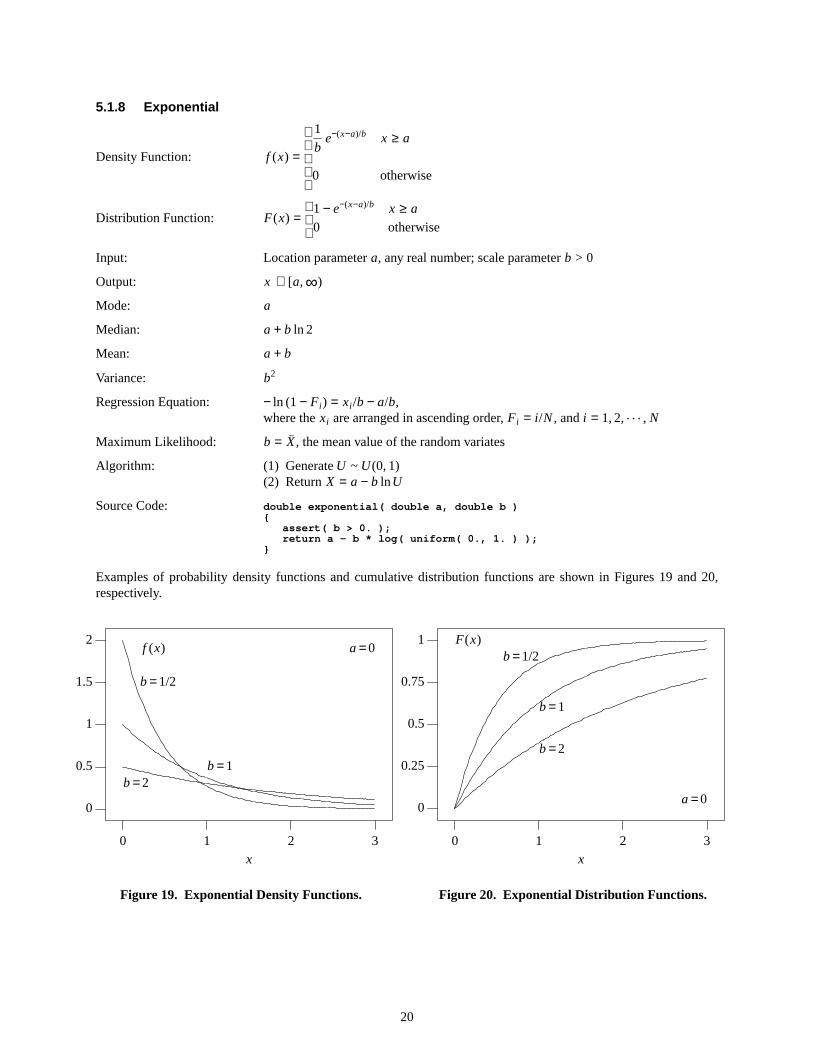
5.1.8 Exponential
Density Function: f (x) =
1
be−(x−a)/b
0
x ≥ a
otherwise
Distribution Function: F(x) =
1 − e−(x−a)/b
0
x ≥ a
otherwise
Input: Location parametera, any real number; scale parameterb > 0
Output: x ∈ [a,∞)
Mode: a
Median: a + b ln 2
Mean: a + b
Variance: b2
Regression Equation: − ln (1 − Fi ) = xi /b − a/b,where thexi are arranged in ascending order, Fi = i /N, and i = 1, 2, . . . , N
Maximum Likelihood: b = X, the mean value of the random variates
Algorithm: (1) GenerateU ~ U(0, 1)(2) Return X = a − b lnU
Source Code: double exponential( double a, double b ){
assert( b > 0. );return a - b * log( uniform( 0., 1. ) );
}
Examples of probability density functions and cumulative distribution functions are shown in Figures 19 and 20,respectively.
0 1 2 3
0
0.5
1
1.5
2
b=1/2
b=1b=2
a =0
x
f (x)
Figure19. Exponential Density Functions.
0 1 2 3x
F(x)
0
0.25
0.5
0.75
1b=1/2
b=1
b=2
a =0
Figure20. Exponential Distrib ution Functions.
20
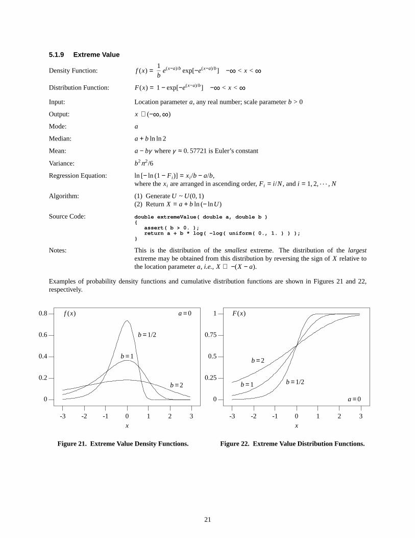
5.1.9 Extreme Value
Density Function: f (x) =1
be(x−a)/b exp[−e(x−a)/b] −∞ < x < ∞
Distribution Function: F(x) = 1 − exp[−e(x−a)/b] −∞ < x < ∞Input: Location parametera, any real number; scale parameterb > 0
Output: x ∈ (−∞,∞)
Mode: a
Median: a + b ln ln 2
Mean: a − bγ whereγ ≈ 0. 57721 is Euler’s constant
Variance: b2π2/6
Regression Equation: ln [− ln (1 − Fi )] = xi /b − a/b,where thexi are arranged in ascending order, Fi = i /N, and i = 1, 2, . . . , N
Algorithm: (1) GenerateU ~ U(0, 1)(2) Return X = a + b ln (− lnU)
Source Code: double extremeValue( double a, double b ){
assert( b > 0. );return a + b * log( -log( uniform( 0., 1. ) ) );
}
Notes: This is the distribution of the smallestextreme. The distribution of the largestextreme may be obtained from this distribution by reversing the sign of X relative tothe location parametera, i.e., X ⇒ −(X − a).
Examples of probability density functions and cumulative distribution functions are shown in Figures 21 and 22,respectively.
-3 -2 -1 0 1 2 3
0
0.2
0.4
0.6
0.8
x
f (x) a =0
b=1/2
b=1
b=2
Figure21. Extreme Value Density Functions.
b=2
b=1 b=1/2
x
F(x)
a =00
0.25
0.5
0.75
1
-3 -2 -1 0 1 2 3
Figure22. Extreme Value Distribution Functions.
21
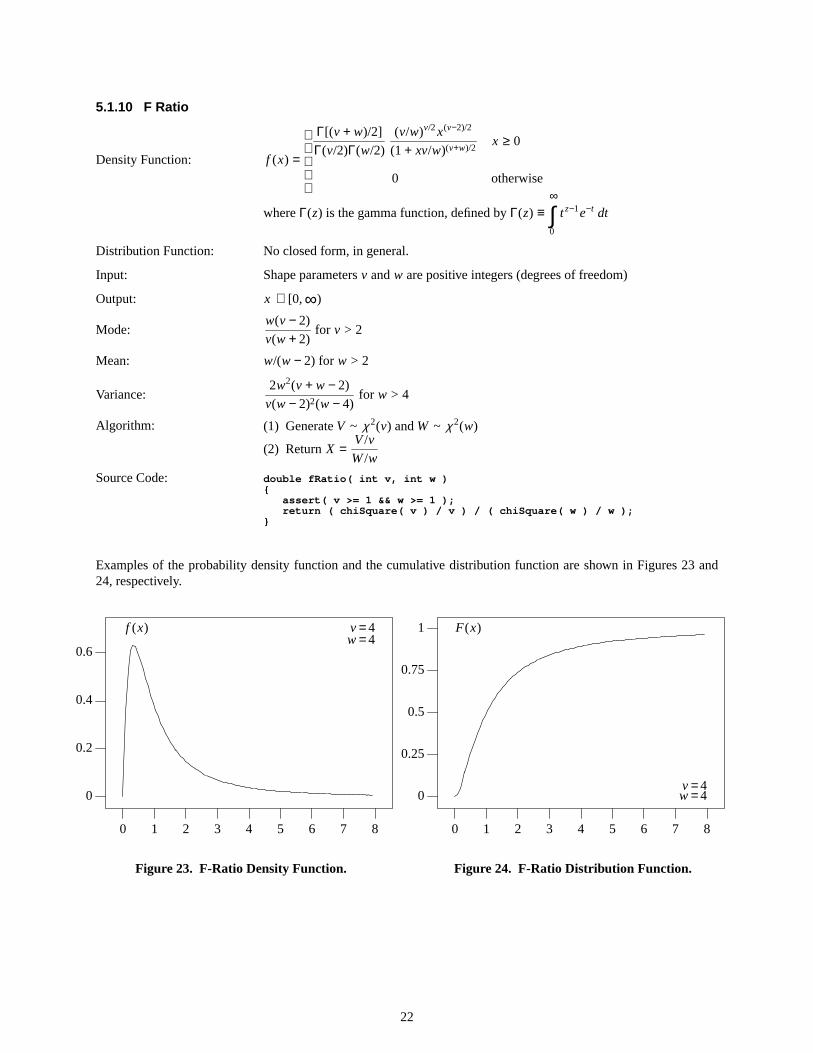
5.1.10 F Ratio
Density Function: f (x) =
Γ[(v + w)/2]
Γ(v/2)Γ(w/2)
(v/w)v/2x(v−2)/2
(1 + xv/w)(v+w)/2
0
x ≥ 0
otherwise
whereΓ(z) is the gamma function, defined byΓ(z) ≡∞
0∫ t z−1e−t dt
Distribution Function: No closed form, in general.
Input: Shapeparametersv andw are positive integers (degrees of freedom)
Output: x ∈ [0,∞)
Mode:w(v − 2)
v(w + 2)for v > 2
Mean: w/(w − 2) for w > 2
Variance:2w2(v + w − 2)
v(w − 2)2(w − 4)for w > 4
Algorithm: (1) GenerateV ~ χ 2(v) andW ~ χ 2(w)
(2) Return X =V/v
W/w
Source Code: double fRatio( int v, int w ){
assert( v >= 1 && w >= 1 );return ( chiSquare( v ) / v ) / ( chiSquare( w ) / w );
}
Examples of the probability density function and the cumulative distribution function are shown in Figures 23 and24, respectively.
f (x) v =4w =4
0 1 2 3 4 5 6 7 8
0
0.2
0.4
0.6
Figure23. F-Ratio Density Function.
F(x)
v =4w =4
0 1 2 3 4 5 6 7 8
0
0.25
0.5
0.75
1
Figure24. F-Ratio Distrib ution Function.
22
5.1.11 Gamma
Density Function: f (x) =
1
Γ(c)b−c(x − a)c−1e−(x−a)/b
0
x > a
otherwise
whereΓ(z) is the gamma function, defined byΓ(z) ≡∞
0∫ t z−1e−t dt
If n is an integer, Γ(n) = (n − 1)!
Distribution Function: No closed form, in general.However, if c is a positive integer, then
F(x) =
1 − e−(x−a)/bc−1
k =0Σ 1
k!
x − a
b
k
0
x > a
otherwise
Input: Location parametera; scale parameterb > 0; shape parameterc > 0
Output: x ∈ [a,∞)
Mode:
a + b(c − 1)
a
if c ≥ 1
if c < 1
Mean: a + bc
Variance: b2c
Algorithm: There are three algorithms (Law and Kelton 1991), depending upon the value of theshape parameterc.
Case 1: c < 1Let β = 1 + c/e.(1) GenerateU1 ~ U(0, 1) and setP = βU1.
If P > 1, go to step 3; otherwise, go to step 2.(2) Set Y = P1/c and generateU2 ~ U(0, 1).
If U2 ≤ e−Y, returnX = Y; otherwise, go back to step 1.(3) Set Y = − ln [(β − P)/c] and generateU2 ~ U(0, 1).
If U2 ≤ Yc−1, returnX = Y; otherwise, go back to step 1.
Case 2: c = 1ReturnX ~ exponential (a, b).
Case 3: c > 1Let α = 1/√ 2c − 1, β = c − ln 4, q = c + 1/α , θ = 4. 5, andd = 1 + lnθ .(1) Generate two IID uniform variates,U1 ~ U(0, 1) andU2 ~ U(0, 1).(2) Set V = α ln [U1/(1 −U1)], Y = ceV , Z = U2
1U2, andW = β + qV − Y.(3) If W + d − θ Z ≥ 0, returnX = Y; otherwise, proceed to step 4.(4) If W ≥ ln Z, returnX = Y; otherwise, go back to step 1.
23
Source Code: double gamma( double a, double b, double c ){
assert( b > 0. && c > 0. );
const double A = 1. / sqrt( 2. * c - 1. );const double B = c - log( 4. );const double Q = c + 1. / A;const double T = 4.5;const double D = 1. + log( T );const double C = 1. + c / M_E;
if ( c < 1. ) {while ( true ) {
double p = C * uniform( 0., 1. );if ( p > 1. ) {
double y = -log( ( C - p ) / c );if ( uniform( 0., 1. ) <= pow( y, c - 1. ) ) return a + b * y;
}else {
double y = pow( p, 1. / c );if ( uniform( 0., 1. ) <= exp( -y ) ) return a + b * y;
}}
}else if ( c == 1.0 ) return exponential( a, b );else {
while ( true ) {double p1 = uniform( 0., 1. );double p2 = uniform( 0., 1. );double v = A * log( p1 / ( 1. - p1 ) );double y = c * exp( v );double z = p1 * p1 * p2;double w = B + Q * v - y;if ( w + D - T * z >= 0. || w >= log( z ) ) return a + b * y;
}}
}
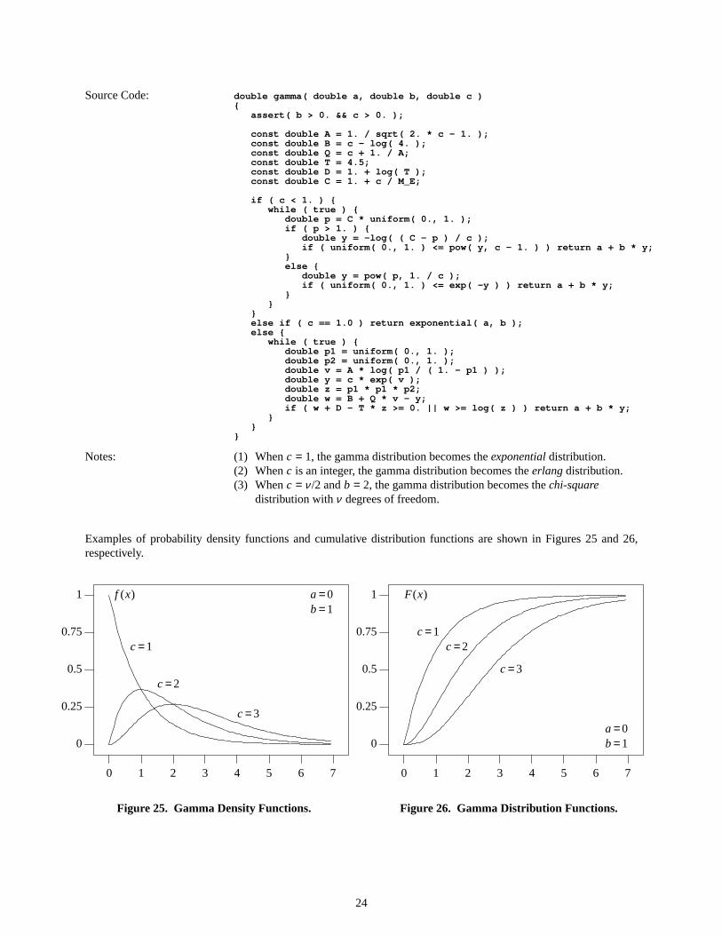
Notes: (1) When c = 1, the gamma distribution becomes theexponentialdistribution.(2) When c is an integer, the gamma distribution becomes theerlangdistribution.(3) When c = ν /2 andb = 2, the gamma distribution becomes thechi-square
distribution withν degrees of freedom.
Examples of probability density functions and cumulative distribution functions are shown in Figures 25 and 26,respectively.
0 1 2 3 4 5 6 7
0
0.25
0.5
0.75
1 f (x) a =0b=1
c =1
c =2
c =3
Figure25. Gamma Density Functions.
0 1 2 3 4 5 6 7
0
0.25
0.5
0.75
1 F(x)
a =0b=1
c =1c =2
c =3
Figure26. Gamma Distrib ution Functions.
24
5.1.12 Laplace (Doub le Exponential)
Density Function: f (x) =1
2bexp
−
|x − a|
b
−∞ < x < ∞
Distribution Function: F(x) =
1
2e(x−a)/b
1 −1
2e−(x−a)/b
x ≤ a
x ≥ a
Input: Location parametera, any real number; scale parameterb > 0
Output: x ∈ (−∞,∞)
Mode: a
Median: a
Mean: a
Variance: 2b2
Regression Equation:
ln (2Fi ) = xi /b − a/b
− ln [2(1 − Fi )] = xi /b − a/b
0 ≤ Fi ≤ 1/2
1/2 ≤ Fi ≤ 1where thexi are arranged in ascending order, Fi = i /N, and i = 1, 2, . . . , N
Algorithm: (1) Generate two IID random variates,U1 ~ U(0, 1) andU2 ~ U(0, 1)
(2) Return X =
a + b lnU2
a − b lnU2
if U1 ≥ 1/2
if U1 < 1/2
Source Code: double laplace( double a, double b ){
assert( b > 0. );
// composition method
if ( bernoulli( 0.5 ) ) return a + b * log( uniform( 0., 1. ) );el se r et ur n a - b * l og( uniform( 0., 1. ) );
}
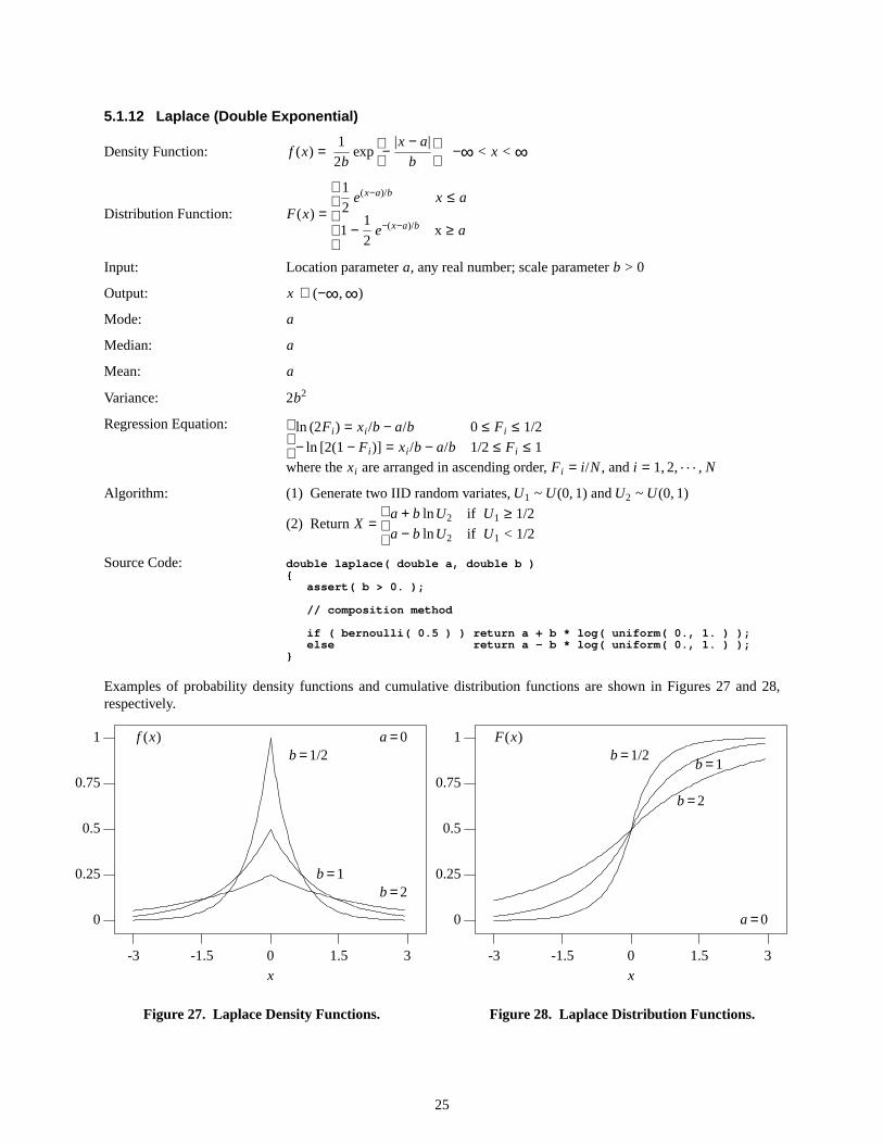
Examples of probability density functions and cumulative distribution functions are shown in Figures 27 and 28,respectively.
b=1/2
b=1b=2
x
f (x) a =0
0
0.25
0.5
0.75
1
-3 -1.5 0 1.5 3
Figure27. LaplaceDensity Functions.
x
F(x)
0
0.25
0.5
0.75
1b=1/2
b=1
b=2
a =0
-3 -1.5 0 1.5 3
Figure28. LaplaceDistrib ution Functions.
25
5.1.13 Logarithmic
Density Function: f (x) =
−1
bln
x − a
b
0
xmin ≤ x ≤ xmax
otherwise
Distribution Function: F(x) =
0
x − a
b
1 − ln
x − a
b
1
x < xmin
xmin ≤ x ≤ xmax
x > xmax
Input: xmin, minimum value of random variable;xmax, maximum value of random variable;location parametera = xmin; scale parameterb = xmax − xmin
Output: x ∈ [xmin, xmax)
Mode: xmin
Mean: xmin +1
4(xmax − xmin)
Variance:7
144(xmax − xmin)2
Algorithm: Based on the convolution formula for the product of two uniform densities,(1) Generate two IID uniform variates,U1 ~ U(0, 1) andU2 ~ U(0, 1)(2) Return X = a + bU1U2
Source Code: double logarithmic( double xMin, double xMax ){
assert( xMin < xMax );
double a = xMin; // location parameterdouble b = xMax - xMin; // scale parameterreturn a + b * uniform( 0., 1. ) * uniform( 0., 1. );
}
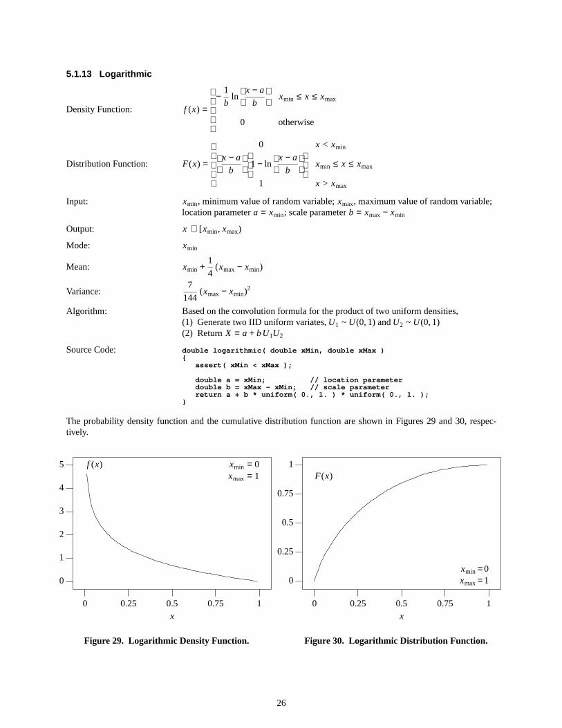
The probability density function and the cumulative distribution function are shown in Figures 29 and 30, respec-tively.
0
1
2
3
4
5 xmin = 0xmax = 1
0 0.25 0.5 0.75 1x
f (x)
Figure29. Logar ithmic Density Function.
xmin =0xmax=1
0 0.25 0.5 0.75 1
0
0.25
0.5
0.75
1
x
F(x)
Figure30. Logar ithmic Distrib ution Function.
26
5.1.14 Logistic
Density Function: f (x) =1
b
e(x−a)/b
[1 + e(x−a)/b]2−∞ < x < ∞
Distribution Function: F(x) =1
1 + e−(x−a)/b−∞ < x < ∞
Input: Location parametera, any real number; scale parameterb > 0
Output: x ∈ (−∞,∞)
Mode: a
Median: a
Mean: a
Variance:π2
3b2
Regression Equation: − ln(F−1i − 1) = xi /b − a/b,
where thexi are arranged in ascending order, Fi = i /N, and i = 1, 2, . . . , N
Algorithm: (1) GenerateU ~ U(0, 1)(2) Return X = a − b ln (U−1 − 1)
Source Code: double logistic( double a, double b ){
assert( b > 0. );return a - b * log( 1. / uniform( 0., 1. ) - 1. );
}
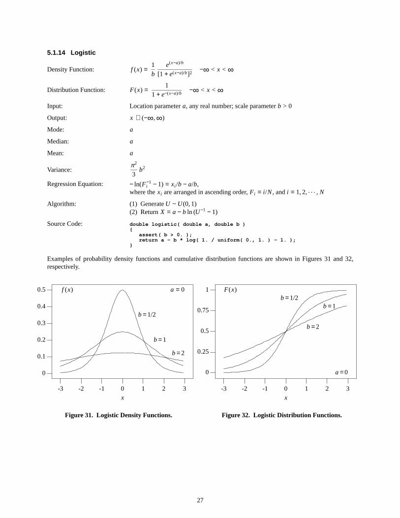
Examples of probability density functions and cumulative distribution functions are shown in Figures 31 and 32,respectively.
0
0.1
0.2
0.3
0.4
0.5 a = 0
b=1/2
b=1
b=2
-3 -2 -1 0 1 2 3x
f (x)
Figure31. Logistic Density Functions.
a =0
b=1/2b=1
b=2
0
0.25
0.5
0.75
1
-3 -2 -1 0 1 2 3x
F(x)
Figure32. Logistic Distrib ution Functions.
27
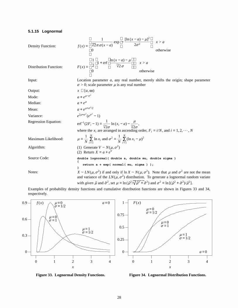
5.1.15 Lognormal
Density Function: f (x) =
1
√ 2π σ (x − a)exp
−
[ln (x − a) − µ]2
2σ 2
0
x > a
otherwise
Distribution Function: F(x) =
1
2
1 + erf
ln (x − a) − µ
√ 2σ
0
x > a
otherwise
Input: Location parameter a, any real number, merely shifts the origin; shape parameterσ > 0; scale parameterµ is any real number
Output: x ∈ [a,∞)
Mode: a + eµ−σ 2
Median: a + eµ
Mean: a + eµ+σ 2/2
Variance: e2µ+σ 2(eσ 2
− 1)
Regression Equation: erf−1(2Fi − 1) =1
√ 2σln (xi − a) −
µ
√ 2σ,
where thexi are arranged in ascending order, Fi = i /N, and i = 1, 2, . . . , N
Maximum Likelihood: µ =1
N
N
i =1Σ ln xi andσ 2 =
1
N
N
i =1Σ (ln xi − µ)2
Algorithm: (1) GenerateV ~ N(µ,σ 2)(2) Return X = a + eV
Source Code: double lognormal( double a, double mu, double sigma ){
return a + exp( normal( mu, sigma ) );}
Notes: X ~ LN(µ,σ 2) if and only if ln X ~ N(µ,σ 2). Note that µ andσ 2 are not the meanand variance of the LN(µ,σ 2) distribution. To generate a lognormal random variate
with given µ̂ and σ̂ 2, set µ = ln (µ̂2/√ µ̂2 + σ̂ 2) andσ 2 = ln [(µ̂2 + σ̂ 2)/ µ̂2].
Examples of probability density functions and cumulative distribution functions are shown in Figures 33 and 34,respectively.
f (x) a =0
µ =0σ =1
µ =0σ =1/2
µ =1σ =1/2
0 1 2 3 4
0
0.3
0.6
0.9
x
Figure33. Lognormal Density Functions.
F(x)
a =0
µ =0σ =1
µ =0σ =1/2
µ =1σ =1/2
0
0.25
0.5
0.75
1
0 1 2 3 4x
Figure34. Lognormal Distrib ution Functions.
28
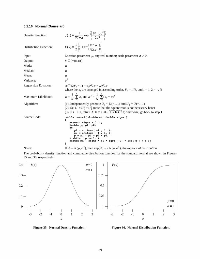
5.1.16 Normal (Gaussian)
Density Function: f (x) =1
√ 2π σexp
−(x − µ)2
2σ 2
Distribution Function: F(x) =1
2
1 + erf
x − µ
√ 2σ
Input: Location parameterµ, any real number; scale parameterσ > 0
Output: x ∈ (−∞,∞)
Mode: µMedian: µMean: µ
Variance: σ 2
Regression Equation: erf−1(2Fi − 1) = xi /√ 2σ − µ/√ 2σ ,where thexi are arranged in ascending order, Fi = i /N, and i = 1, 2, . . . , N
Maximum Likelihood: µ =1
N
N
i =1Σ xi andσ 2 =
1
N
N
i =1Σ (xi − µ)2
Algorithm: (1) Independently generateU1 ~ U(−1, 1) andU2 ~ U(−1, 1)(2) Set U = U2
1 +U22 (note that the square root is not necessary here)
(3) If U < 1, returnX = µ + σU1 √ −2lnU /U ; otherwise, go back to step 1
Source Code: double normal( double mu, double sigma ){
assert( sigma > 0. );double p, p1, p2;do {
p1 = uniform( -1., 1. );p2 = uniform( -1., 1. );p = p1 * p1 + p2 * p2;
} while ( p >= 1. );return mu + sigma * p1 * sqrt( -2. * log( p ) / p );
}
Notes: If X ~ N(µ,σ 2), then exp(X) ~ LN(µ,σ 2), thelognormal distribution.
The probability density function and cumulative distribution function for the standard normal are shown in Figures35 and 36, respectively.
0
0.1
0.2
0.3
0.4 f (x) µ =0
σ =1
-3 -2 -1 0 1 2 3x
Figure35. Normal Density Function.
F(x)
µ =0
σ =10
0.25
0.5
0.75
1
-3 -2 -1 0 1 2 3x
Figure36. Normal Distrib ution Function.
29

5.1.17 Parabolic
Density Function: f (x) =3
4b1 − (
x − a
b)2
xmin ≤ x ≤ xmax
Distribution Function: F(x) =(a + 2b − x)(x − a + b)2
4b3xmin ≤ x ≤ xmax
Input: xmin, minimum value of random variable;xmax, maximum value of random variable;location parametera = (xmin + xmax)/2; scale parameterb = (xmax − xmin)/2
Output: x ∈ [xmin, xmax)
Mode: (xmin + xmax)/2
Median: (xmin + xmax)/2
Mean: (xmin + xmax)/2
Variance: (xmax − xmin)2/20
Algorithm: Uses theacceptance-rejectionmethod on the above density functionf (x)
Source Code: // function to call for the Monte Carlo samplingdouble parabola( double x, double xMin, double xMax ){
if ( x < xMin || x > xMax ) return 0.0;
double a = 0.5 * ( xMin + xMax ); // location parameterdouble b = 0.5 * ( xMax - xMin ); // scale parameterdouble yMax = 3. / ( 4. * b );
return yMax * ( 1. - ( x - a ) * ( x - a ) / ( b * b ) );}
// function which generates parabolic distributiondouble parabolic( double xMin, double xMax ){
assert( xMin < xMax );
double a = 0.5 * ( xMin + xMax ); // location parameterdouble yMax = parabola( a, xMin, xMax ); // max function range
return userSpecified( parabola, xMin, xMax, 0., yMax );}
Notes: The parabolic distribution is a special case of the betadistribution (when v = w = 2).
The probability density function and the cumulative distribution function are shown in Figures 37 and 38, respec-tively.
0
0.5
1
1.5
0 0.25 0.5 0.75 1x
f (x) xmin =0xmax=1
Figure37. Parabolic Density Function.
xmin =0xmax=1
x
F(x)
0
0.25
0.5
0.75
1
0 0.25 0.5 0.75 1
Figure38. Parabolic Distribution Function.
30
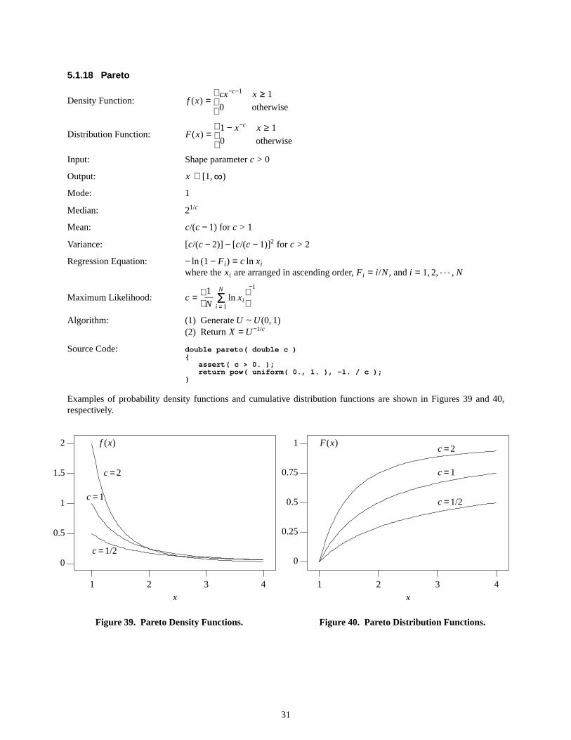
5.1.18 Pareto
Density Function: f (x) =
cx−c−1
0
x ≥ 1
otherwise
Distribution Function: F(x) =
1 − x−c
0
x ≥ 1
otherwise
Input: Shapeparameterc > 0
Output: x ∈ [1,∞)
Mode: 1
Median: 21/c
Mean: c/(c − 1) for c > 1
Variance: [c/(c − 2)] − [c/(c − 1)]2 for c > 2
Regression Equation: − ln (1 − Fi ) = c ln xi
where thexi are arranged in ascending order, Fi = i /N, and i = 1, 2, . . . , N
Maximum Likelihood: c =
1
N
N
i =1Σ ln xi
−1
Algorithm: (1) GenerateU ~ U(0, 1)(2) Return X = U−1/c
Source Code: double pareto( double c ){
assert( c > 0. );return pow( uniform( 0., 1. ), -1. / c );
}
Examples of probability density functions and cumulative distribution functions are shown in Figures 39 and 40,respectively.
1 2 3 4
0
0.5
1
1.5
2
c =2
c =1
c =1/2
x
f (x)
Figure39. Pareto Density Functions.
1 2 3 4x
F(x)
0
0.25
0.5
0.75
1c =2
c =1
c =1/2
Figure40. Pareto Distribution Functions.
31

5.1.19 Pearson’ s Type 5 (Inver ted Gamma)
Density Function: f (x) =
x−(c+1)e−b/x
b−cΓ(c)
0
if x > 0
otherwise
whereΓ(z) is the gamma function, defined byΓ(z) ≡∞
0∫ t z−1e−t dt
Distribution Function: F(x) =
Γ(c, b/x)
Γ(c)
0
if x > 0
otherwise
whereΓ(a, z) is the incomplete gamma function, defined byΓ(a, z) ≡∞
z∫ ta−1e−t dt
Input: Scaleparameterb > 0; shape parameterc > 0
Output: x ∈ [0,∞)
Mode: b/(c + 1)
Mean: b/(c − 1) for c > 1
Variance: b2/[(c − 1)2(c − 2)] for c > 2
Algorithm: (1) GenerateY ~ gamma (0, 1/b, c)(2) Return X = 1/Y
Source Code: double pearson5( double b, double c ){
assert( b > 0. && c > 0. );return 1. / gamma( 0., 1. / b , c);
}
Notes: X ~ PearsonType5(b, c) if and only if 1/X ~ gamma (0, 1/b, c). Thus, the PearsonType 5 distribution is sometimes called theinverted gamma distribution.
Examples of probability density functions and cumulative distribution functions are shown in Figures 41 and 42,respectively.
c =2
c =1
f (x)
0 1 2 3 4 5
0
0.5
1
1.5
Figure41. Pearson Type 5 Density Functions.
F(x)
c =2
c =1
0 1 2 3 4 5
0
0.25
0.5
0.75
1
Figure42. Pearson Type 5 Distribution Functions.
32
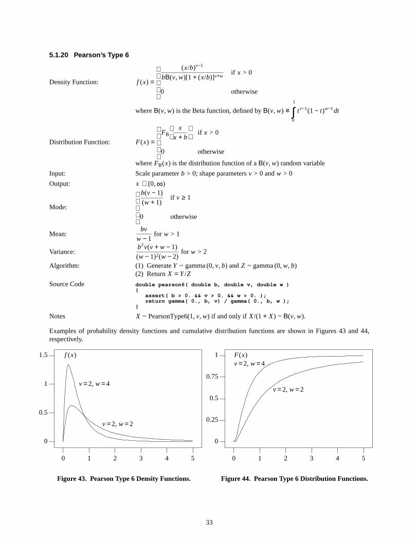
5.1.20 Pearson’ s Type 6
Density Function: f (x) =
(x/b)v−1
bΒ(v, w)[1 + (x/b)]v+w
0
if x > 0
otherwise
whereΒ(v, w) is the Beta function, defined byΒ(v, w) ≡1
0∫ tv−1(1 − t)w−1dt
Distribution Function: F(x) =
FΒ
x
x + b
0
if x > 0
otherwise
whereFΒ(x) is the distribution function of aΒ(v, w) random variable
Input: Scaleparameterb > 0; shape parametersv > 0 andw > 0
Output: x ∈ [0,∞)
Mode:
b(v − 1)
(w + 1)
0
if v ≥ 1
otherwise
Mean:bv
w − 1for w > 1
Variance:b2v(v + w − 1)
(w − 1)2(w − 2)for w > 2
Algorithm: (1) GenerateY ~ gamma (0, v, b) and Z ~ gamma (0, w, b)(2) Return X = Y/Z
Source Code double pearson6( double b, double v, double w ){
assert( b > 0. && v > 0. && w > 0. );return gamma( 0., b, v) / gamma( 0., b, w );
}
Notes X ~ PearsonType6(1,v, w) if and only if X/(1 + X) ~ Β(v, w).
Examples of probability density functions and cumulative distribution functions are shown in Figures 43 and 44,respectively.
v =2, w =4
v =2, w =2
f (x)
0 1 2 3 4 5
0
0.5
1
1.5
Figure43. Pearson Type 6 Density Functions.
F(x)v =2, w =4
v =2, w =2
0 1 2 3 4 5
0
0.25
0.5
0.75
1
Figure44. Pearson Type 6 Distribution Functions.
33
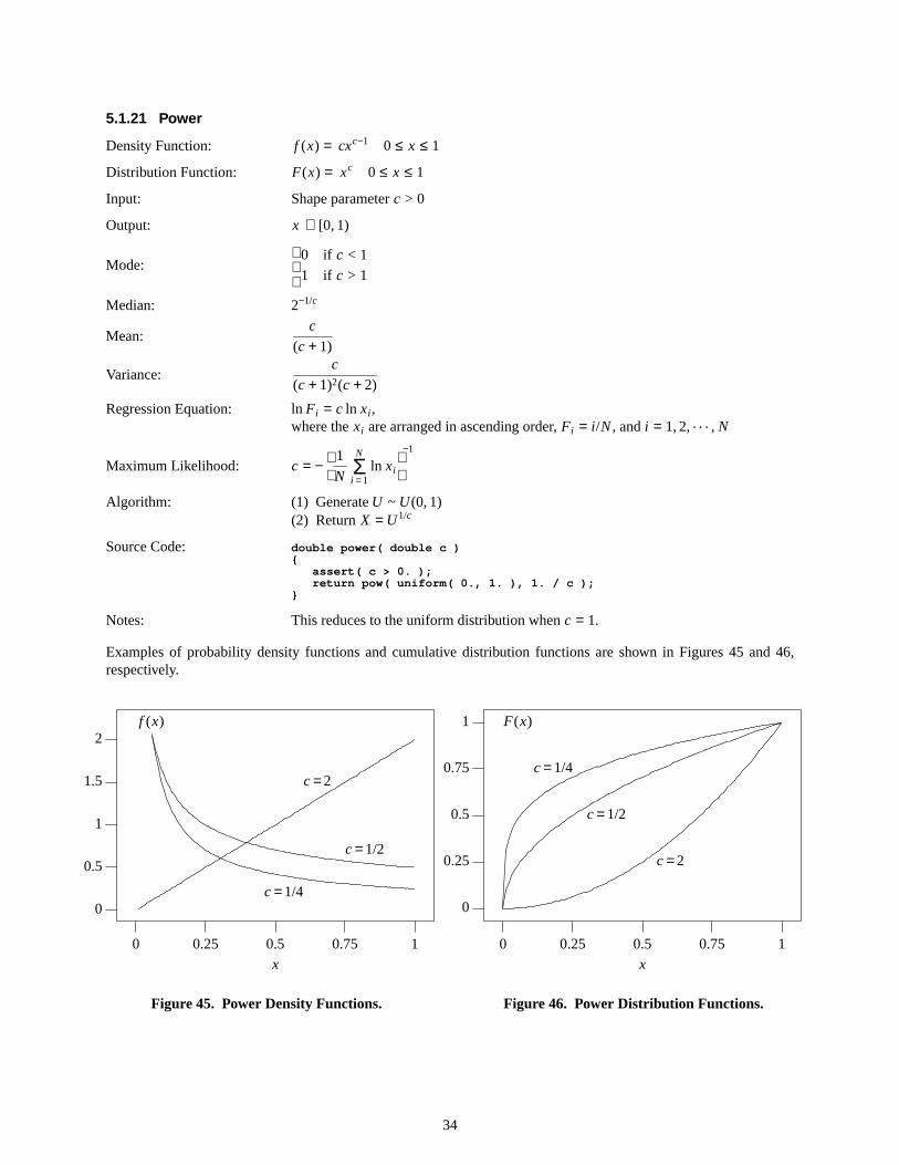
5.1.21 Power
Density Function: f (x) = cxc−1 0 ≤ x ≤ 1
Distribution Function: F(x) = xc 0 ≤ x ≤ 1
Input: Shapeparameterc > 0
Output: x ∈ [0, 1)
Mode:
0
1
if c < 1
if c > 1
Median: 2−1/c
Mean:c
(c + 1)
Variance:c
(c + 1)2(c + 2)
Regression Equation: ln Fi = c ln xi ,where thexi are arranged in ascending order, Fi = i /N, and i = 1, 2, . . . , N
Maximum Likelihood: c = −
1
N
N
i =1Σ ln xi
−1
Algorithm: (1) GenerateU ~ U(0, 1)(2) Return X = U1/c
Source Code: double power( double c ){
assert( c > 0. );return pow( uniform( 0., 1. ), 1. / c );
}
Notes: This reduces to the uniform distribution whenc = 1.
Examples of probability density functions and cumulative distribution functions are shown in Figures 45 and 46,respectively.
0
0.5
1
1.5
2
c =1/2
c =1/4
c =2
0 0.25 0.5 0.75 1x
f (x)
Figure45. Power Density Functions.
x
F(x)
0
0.25
0.5
0.75
1
0 0.25 0.5 0.75 1
c =1/4
c =1/2
c =2
Figure46. Power Distribution Functions.
34
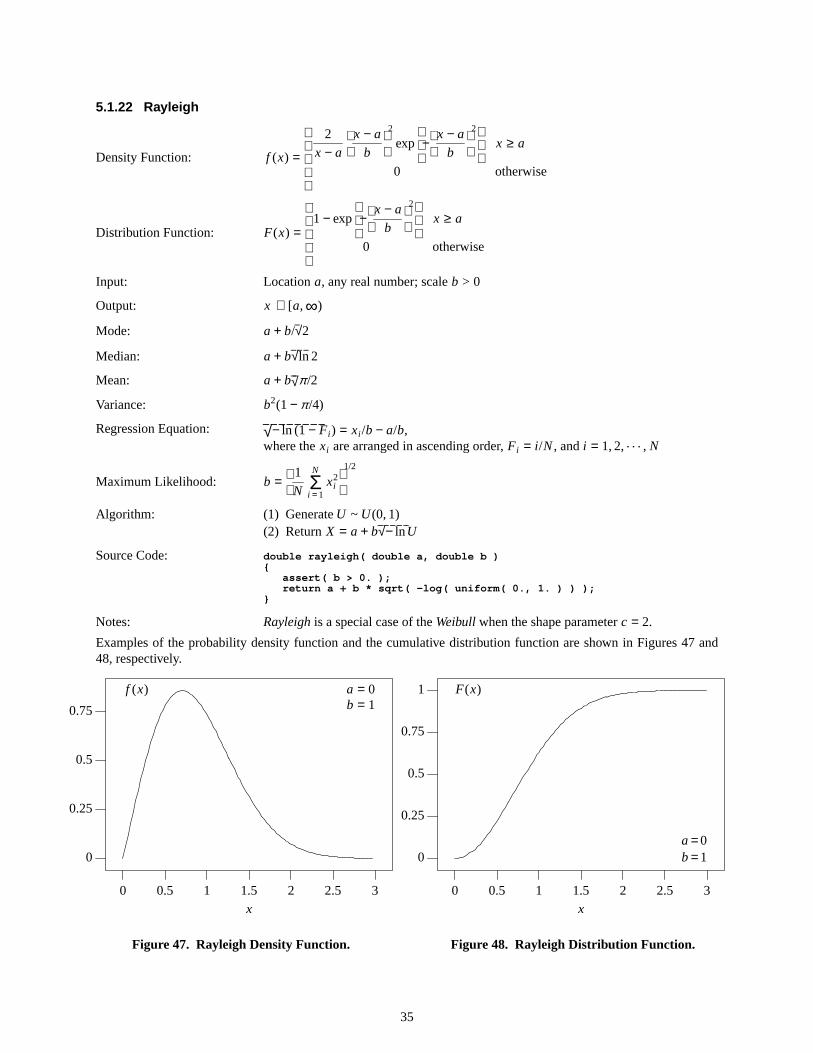
5.1.22 Rayleigh
Density Function: f (x) =
2
x − a
x − a
b
2
exp−
x − a
b
2
0
x ≥ a
otherwise
Distribution Function: F(x) =
1 − exp−
x − a
b
2
0
x ≥ a
otherwise
Input: Location a, any real number; scaleb > 0
Output: x ∈ [a,∞)
Mode: a + b/√ 2
Median: a + b√ ln 2
Mean: a + b√ π/2
Variance: b2(1 − π/4)
Regression Equation: √ − ln (1 − Fi ) = xi /b − a/b,where thexi are arranged in ascending order, Fi = i /N, and i = 1, 2, . . . , N
Maximum Likelihood: b =
1
N
N
i =1Σ x2
i
1/2
Algorithm: (1) GenerateU ~ U(0, 1)(2) Return X = a + b√ − lnU
Source Code: double rayleigh( double a, double b ){
assert( b > 0. );return a + b * sqrt( -log( uniform( 0., 1. ) ) );
}
Notes: Rayleighis a special case of theWeibull when the shape parameterc = 2.
Examples of the probability density function and the cumulative distribution function are shown in Figures 47 and48, respectively.
a = 0b = 1
f (x)
0
0.25
0.5
0.75
0 0.5 1 1.5 2 2.5 3x
Figure47. Rayleigh Density Function.
a =0b=1
F(x)
0
0.25
0.5
0.75
1
0 0.5 1 1.5 2 2.5 3x
Figure48. Rayleigh Distrib ution Function.
35
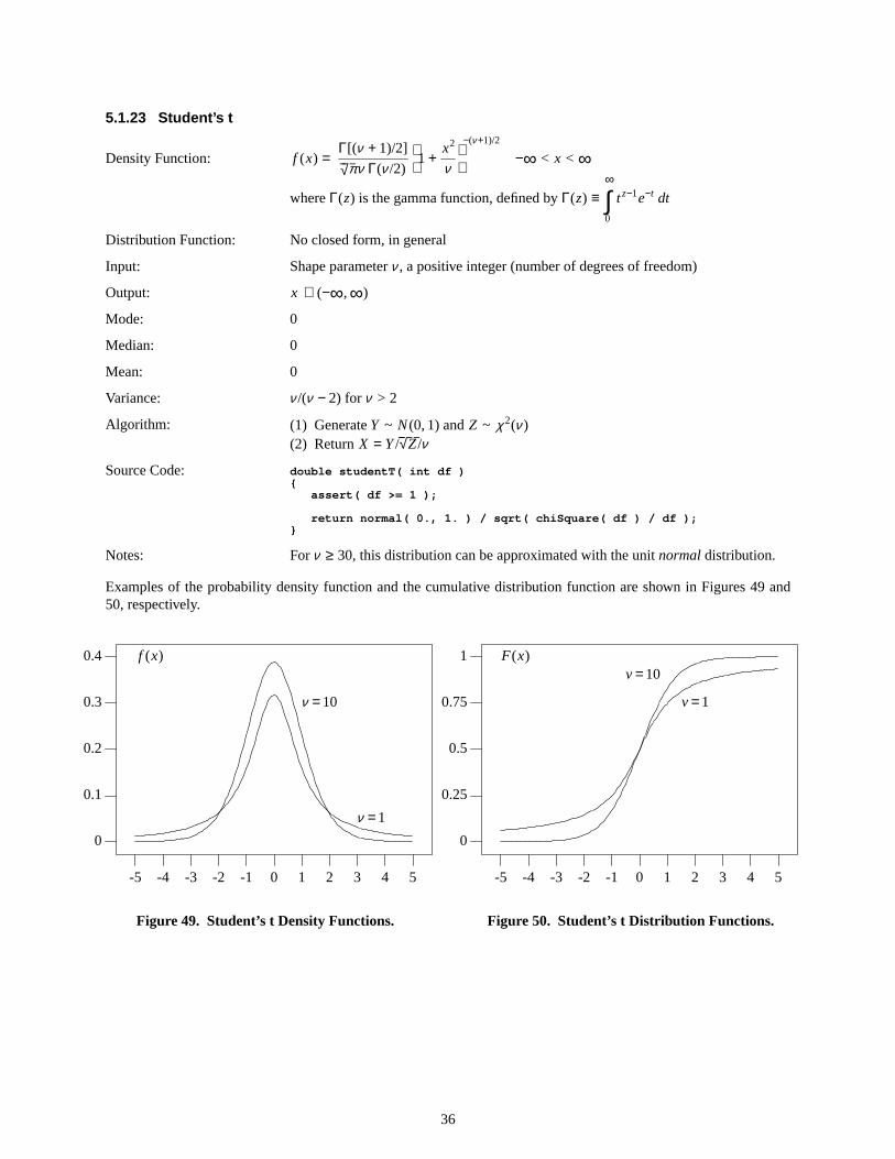
5.1.23 Student’s t
Density Function: f (x) =Γ[(ν + 1)/2]
√ πν Γ(ν /2)1 +
x2
ν
−(ν +1)/2
−∞ < x < ∞
whereΓ(z) is the gamma function, defined byΓ(z) ≡∞
0∫ t z−1e−t dt
Distribution Function: No closed form, in general
Input: Shapeparameterν , apositive integer (number of degrees of freedom)
Output: x ∈ (−∞,∞)
Mode: 0
Median: 0
Mean: 0
Variance: ν /(ν − 2) forν > 2
Algorithm: (1) GenerateY ~ N(0, 1) andZ ~ χ 2(ν )(2) Return X = Y/√ Z/ν
Source Code: double studentT( int df ){
assert( df >= 1 );
return normal( 0., 1. ) / sqrt( chiSquare( df ) / df );}
Notes: For ν ≥ 30, this distribution can be approximated with the unitnormaldistribution.
Examples of the probability density function and the cumulative distribution function are shown in Figures 49 and50, respectively.
f (x)
ν =10
ν =1
-5 -4 -3 -2 -1 0 1 2 3 4 5
0
0.1
0.2
0.3
0.4
Figure49. Student’s t Density Functions.
F(x)
v =1
v =10
-5 -4 -3 -2 -1 0 1 2 3 4 5
0
0.25
0.5
0.75
1
Figure50. Student’s t Distrib ution Functions.
36
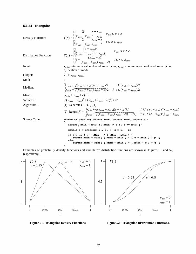
5.1.24 Triangular
Density Function: f (x) =
2
xmax − xmin
x − xmin
c − xmin2
xmax − xmin
xmax − x
xmax − c
xmin ≤ x ≤ c
c ≤ x ≤ xmax
Distribution Function: F(x) =
(x − xmin)2
(xmax − xmin)(c − xmin)
1 −(xmax − x)2
(xmax − xmin)(xmax − c)
xmin ≤ x ≤ c
c ≤ x ≤ xmax
Input: xmin, minimum value of random variable;xmax, maximum value of random variable;c, location of mode
Output: x ∈ [xmin, xmax)
Mode: c
Median:
xmin + √ (xmax − xmin)(c − xmin)/2
xmax − √ (xmax − xmin)(xmax − c)/2
if c ≥ (xmin + xmax)/2
if c ≤ (xmin + xmax)/2
Mean: (xmin + xmax + c) / 3
Variance: [3(xmax − xmin)2 + (xmin + xmax − 2c)2] / 72
Algorithm: (1) GenerateU ~ U(0, 1)
(2) Return X =
xmin + √ (xmax − xmin)(c − xmin)U
xmax − √ (xmax − xmin)(xmax − c)(1 −U)
if U ≤ (c − xmin)/(xmax − xmin)
if U > (c − xmin)/(xmax − xmin)
Source Code: double triangular( double xMin, double xMax, double c ){
assert( xMin < xMax && xMin <= c && c <= xMax );
double p = uniform( 0., 1. ), q = 1. - p;
if ( p <= ( c - xMin ) / ( xMax - xMin ) )return xMin + sqrt( ( xMax - xMin ) * ( c - xMin ) * p );
elsereturn xMax - sqrt( ( xMax - xMin ) * ( xMax - c ) * q );
}
Examples of probability density functions and cumulative distribution funtions are shown in Figures 51 and 52,respectively.
c = 0. 5c = 0. 25
xmin = 0xmax = 1
0 0.25 0.5 0.75 1
0
1
2
x
f (x)
Figure51. Triangular Density Functions.
c = 0. 5c = 0. 25
0 0.25 0.5 0.75 1
0
0.5
1
xmin = 0xmax = 1
x
F(x)
Figure52. Triangular Distrib ution Functions.
37

5.1.25 Uniform
Density Function: f (x) =
1
xmax − xmin
0
xmin < x < xmax
otherwise
Distribution Function: F(x) =
0x − xmin
xmax − xmin1
x < xmin
xmin < x < xmax
xmax < x
Input: xmin, minimum value of random variable;xmax, maximum value of random variable
Output: x ∈ [xmin, xmax)
Mode: Does not uniquely exist
Median: (xmin + xmax)/2
Mean: (xmin + xmax)/2
Variance: (xmax − xmin)2/12
Algorithm: (1) GenerateU ~ U(0, 1)(2) Return X = xmin + (xmax − xmin)U
Source Code: double uniform( double xMin, double xMax ){
assert( xMin < xMax );return xMin + ( xMax - xMin ) * _u();
}
Notes: (1) Thesource code for_u() referenced above is giv en in section 6.(2) The uniform distribution is the basis for most distributions in the Random class.(3) Theuniform distribution is a special case of thebetadistribution
(whenv = w = 1).
The probability density function and the cumulative distribution function are shown in Figures 53 and 54, respec-tively.
0
1
2
0 0.25 0.5 0.75 1
f (x) xmin = 0xmax = 1
x
Figure53. Uniform Density Function.
0
0.25
0.5
0.75
1
0 0.25 0.5 0.75 1
F(x)
xmin = 0xmax = 1
x
Figure54. Uniform Distrib ution Function.
38
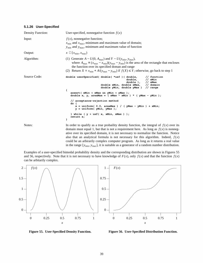
5.1.26 User-Specified
Density Function: User-specified, nonnegative function f (x)
Input: f (x), nonnegative function;xmin andxmax, minimum and maximum value of domain;ymin andymax, minimum and maximum value of function
Output: x ∈ [xmin, xmax)
Algorithm: (1) Generate A ~ U(0, Amax) andY ~ U(ymin, ymax),whereAmax ≡ (xmax − xmin)(ymax − ymin) is the area of the rectangle that enclosesthe function over its specified doman and range
(2) Return X = xmin + A/(ymax − ymin) if f (X) ≤ Y; otherwise, go back to step 1
Source Code: double userSpecified( double( *usf )( double, // functiondoubl e, / / xMindouble ), // xMax
double xMin, double xMax, // domaindouble yMin, double yMax ) // range
{assert( xMin < xMax && yMin < yMax );double x, y, areaMax = ( xMax - xMin ) * ( yMax - yMin );
// acceptance-rejection methoddo {
x = uniform( 0.0, areaMax ) / ( yMax - yMin ) + xMin;y = uniform( yMin, yMax );
} while ( y > usf( x, xMin, xMax ) );return x;
}
Notes: In order to qualify as a true probaility density function, the integral of f (x) over itsdomain must equal 1, but that is not a requirement here. As long as f (x) is nonneg-ative over its specified domain, it is not necessary to normalize the function. Noticealso that an analytical formula is not necessary for this algorithm. Indeed, f (x)could be an arbirarily complex computer program. As long as it returns a real valuein the range [ymin, ymax], it is suitable as a generator of a random number distribution.
Examples of a user-specified bimodal probability density and the corresponding distribution are shown in Figures 55and 56, respectively. Note that it is not necessary to have knowledge of F(x), only f (x) and that the function f (x)can be arbitarily complex.
0 0.25 0.5 0.75 1
0
0.5
1
1.5
2
x
f (x)
Figure55. User-Specified Density Function.
0
0.25
0.5
0.75
1
0 0.25 0.5 0.75 1x
F(x)
Figure56. User-Specified Distribution Function.
39
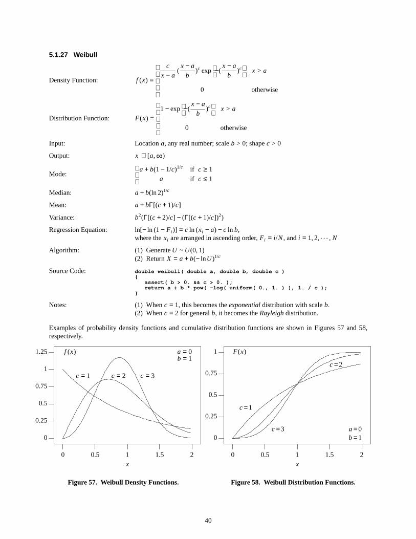
5.1.27 Weibull
Density Function: f (x) =
c
x − a(x − a
b)c exp
−(
x − a
b)c
0
x > a
otherwise
Distribution Function: F(x) =
1 − exp −(
x − a
b)c
0
x > a
otherwise
Input: Location a, any real number; scaleb > 0; shapec > 0
Output: x ∈ [a,∞)
Mode:
a + b(1 − 1/c)1/c
a
if c ≥ 1
if c ≤ 1
Median: a + b(ln 2)1/c
Mean: a + bΓ[(c + 1)/c]
Variance: b2(Γ[(c + 2)/c] − (Γ[(c + 1)/c])2)
Regression Equation: ln[− ln (1 − Fi )] = c ln (xi − a) − c ln b,where thexi are arranged in ascending order, Fi = i /N, and i = 1, 2, . . . , N
Algorithm: (1) GenerateU ~ U(0, 1)(2) Return X = a + b(− lnU)1/c
Source Code: double weibull( double a, double b, double c ){
assert( b > 0. && c > 0. );return a + b * pow( -log( uniform( 0., 1. ) ), 1. / c );
}
Notes: (1) When c = 1, this becomes theexponentialdistribution with scaleb.(2) When c = 2 for generalb, it becomes theRayleighdistribution.
Examples of probability density functions and cumulative distribution functions are shown in Figures 57 and 58,respectively.
c = 1 c = 2 c = 3
a = 0b = 1
0
0.25
0.5
0.75
1
1.25
0 0.5 1 1.5 2
f (x)
x
Figure57. Weibull Density Functions.
c =1
c =2
c =3 a =0b=1
F(x)
0 0.5 1 1.5 2
0
0.25
0.5
0.75
1
x
Figure58. Weibull Distrib ution Functions.
40
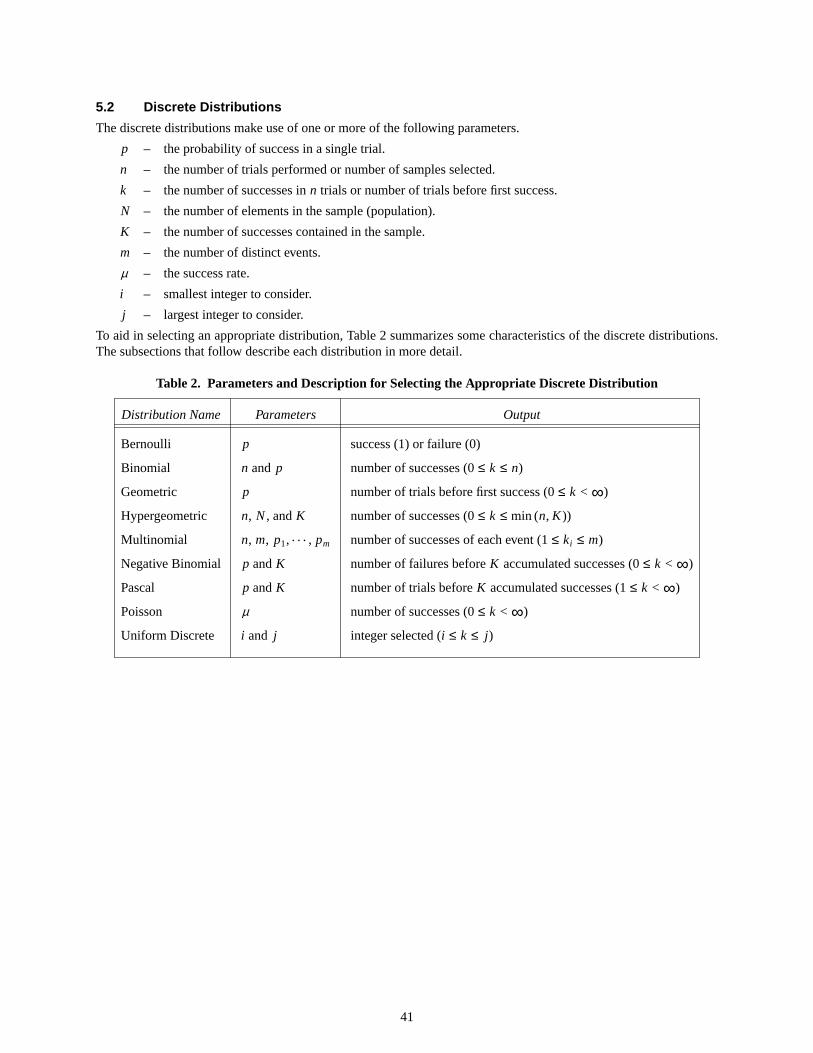
5.2 Discrete Distrib utions
The discrete distributions makeuse of one or more of the following parameters.
p – the probability of success in a single trial.
n – the number of trials performed or number of samples selected.
k – the number of successes inn trials or number of trials before first success.
N – the number of elements in the sample (population).
K – the number of successes contained in the sample.
m – the number of distinct events.
µ – the success rate.
i – smallest integer to consider.
j – largest integer to consider.
To aid in selecting an appropriate distribution, Table 2 summarizes some characteristics of the discrete distributions.The subsections that follow describe each distribution in more detail.
Table 2. Parameters and Description for Selecting the Appropriate Discrete Distribution
Distribution Name Parameters Output
Bernoulli p success (1) or failure (0)
Binomial n and p number of successes (0≤ k ≤ n)
Geometric p number of trials before first success (0≤ k < ∞)
Hypergeometric n, N, and K number of successes (0≤ k ≤ min (n, K ))
Multinomial n, m, p1, . . . , pm number of successes of each event (1 ≤ ki ≤ m)
Negative Binomial p andK number of failures beforeK accumulated successes (0≤ k < ∞)
Pascal p andK number of trials beforeK accumulated successes (1≤ k < ∞)
Poisson µ number of successes (0≤ k < ∞)
Uniform Discrete i and j integer selected (i ≤ k ≤ j )
41
5.2.1 Bernoulli
A Bernoulli trial is the simulation of a probabilistic event with two possible outcomes: success (X = 1) or failure(X = 0), where the probability of success on a single trial is p. It forms the basis for a number of other discrete dis-tributions.
Density Function: f (k) =
1 − p
p
if
if
0
1
Distribution Function: F(k) =
1 − p
1
if
if
0 ≤ k < 1
k ≥ 1
Input: Probability of event, p, where 0≤ p ≤ 1
Output: k ∈ { 0, 1}
Mode:
0
0, 1
1
if
if
if
p < 1/2
1/2
p > 1/2
Mean p
Variance: p(1 − p)
Maximum Likelihood: p = X, the mean value of the IID Bernoulli variates
Algorithm: (1) GenerateU ~ U(0, 1)
(2) Return X =
1
0
if U < p
if U ≥ p
Source Code: bool bernoulli( double p ){
assert( 0. <= p && p <= 1. );
return uniform( 0., 1. ) < p;}
Notes: (1) Notice that if p is strictly zero, then the algorithm above always returnsX = 0,and if p is strictly one, it always returnsX = 1, as it should.
(2) Thesum ofn IID Bernoulli variates generates abinomialdistribution.Thus, the Bernoulli distribution is a special case of the binomial distributionwhen the number of trials is one.
(3) Thenumber of failures before the first success in a sequence of Bernoulli trialsgenerates ageometricdistribution.
(4) Thenumber of failures before the firstn successes in a sequence of Bernoullitrials generates anegative binomialdistribution.
(5) Thenumber of Bernoulli trials required to produce the firstn successesgenerates aPascaldistribution.
42

5.2.2 Binomial
The binomial distribution represents the probability of k successes in n independent Bernoulli trials, where the prob-ability of success in a single trial isp.
Density Function: f (k) =
n
k
pk(1 − p)n−k
0
k ∈ { 0, 1, . . . , n}
otherwise
Distribution Function: F(k) =
k
i = 0Σ
n
i
pi (1 − p)n−i
1
0 ≤ k ≤ n
k > n
where thebinomial coefficient
n
i
=n!
i !(n − i)!
Input: Probability of event, p, where 0≤ p ≤ 0, and number of trials,n ≥ 1
Output: Thenumber of successesk ∈ { 0, 1, . . . , n}
Mode: The integerk that satisfiesp(n + 1) − 1 ≤ k ≤ p(n + 1)
Mean: np
Variance: np(1 − p)
Maximum Likelihood: p = X/n, whereX is the mean of the random variates
Algorithm: (1) Generate n IID Bernoulli trials Xi ~ Bernoulli(p), wherei = 1,. . . , n(2) Return X = X1 + . . . + Xn
Source Code: int binomial( int n, double p ){
assert( 0. <= p && p <= 1. && n >= 1 );int sum = 0;for ( int i = 0; i < n; i++ ) sum += bernoulli( p );return sum;
}
Notes: (1) Thebinomial reduces to theBernoulliwhenn = 1.(2) Poisson(np) approximates binomial(n, p) when p << 1 andn >> 1.(3) For large n, the binomial can be approximated by N(np, np), provided np > 5
and 0.1 ≤ p ≤ 0. 9 — and for all values ofp whennp > 25.
Examples of the probability density function and the cumulative distribution function are shown in Figures 59 and60, respectively.
0
0.1
0.2
0.3p = 0. 1n = 20
f (k)
Number of Successes,k
0 1 2 3 4 5 6 7 8 9 10
Figure59. Binomial Density Function.
p = 0. 1n = 20
F(k)
Number of Successes,k
0
0.25
0.5
0.75
1
0 1 2 3 4 5 6 7 8 9 10
Figure60. Binomial Distrib ution Function.
43

5.2.3 Geometric
The geometric distribution represents the probability of obtaining k failures before the first success in independentBernoulli trials, where the probability of success in a single trial is p. Or, to state it in a slightly different way, it isthe probability of having to performk trialsbeforeachieving a success (i.e., the success itself is not counted).
Density Function: f (k) =
p(1 − p)k
0
k ∈ { 0, 1, . . . }
otherwise
Distribution Function: F(k) =
1 − (1 − p)k+1
0
k ≥ 0
otherwise
Input: Probability of event, p, where 0< p < 1
Output Number of trials before a successk ∈ { 0, 1, . . . }
Mode: 0
Mean: (1 − p)/p
Variance (1 − p)/p2
Maximum Likelihood: p = 1/(1+ X), whereX is the mean value of the IID geometric variates
Algorithm: (1) GenerateU ~ U(0, 1)(2) Return X = int ( lnU / ln (1 − p) )
Source Code: int geometric( double p ){
assert( 0. < p && p < 1. );return int( log( uniform( 0., 1. ) ) / log( 1. - p ) );
}
Notes: (1) A word of caution: There are two different definitions that are in common usefor the geometric distribution. Theother definition is the number of failuresupto and includingthe first success.
(2) Thegeometric distribution is the discrete analog of the exponential distribution.(3) If X1, X2, . . . is a sequence of independent Bernoulli(p) random variates and
X = min { i ∋ Xi = 1} − 1, thenX ~ geometric (p).
Examples of the probability density function and the cumulative distribution function are shown in Figures 61 and62, respectively.
0
0.1
0.2
0.3
0.4
0.5
0 1 2 3 4 5 6 7 8 9 10
f (k) p = 1/2
k
Figure61. Geometr ic Density Function.
0
0.25
0.5
0.75
1
0 1 2 3 4 5 6 7 8 9 10
F(x)
p = 1/2
x
Figure62. Geometr ic Distrib ution Function.
44
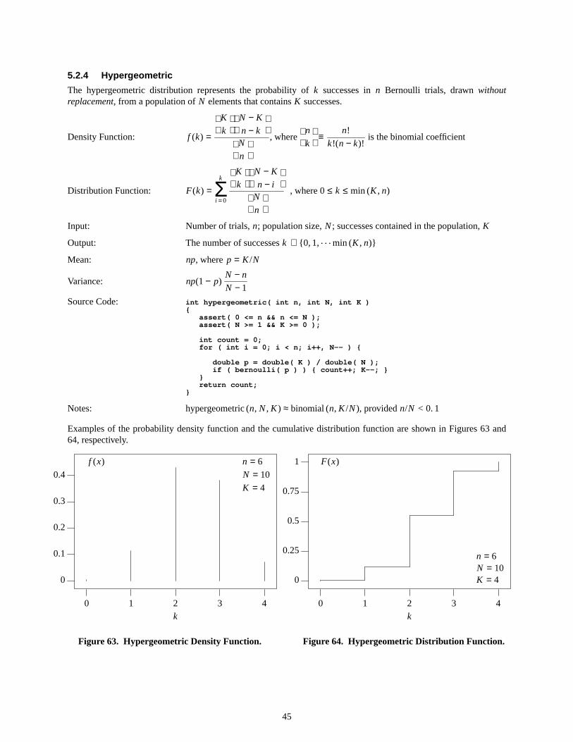
5.2.4 Hypergeometric
The hypergeometric distribution represents the probability of k successes in n Bernoulli trials, drawn withoutreplacement, from a population ofN elements that containsK successes.
Density Function: f (k) =
K
k
N − K
n − k
N
n
, where
n
k
≡n!
k!(n − k)!is the binomial coefficient
Distribution Function: F(k) =k
i =0Σ
K
k
N − K
n − i
N
n
, where 0≤ k ≤ min (K , n)
Input: Number of trials,n; population size,N; successes contained in the population,K
Output: Thenumber of successesk ∈ { 0, 1, . . . min (K , n)}
Mean: np, wherep = K /N
Variance: np(1 − p)N − n
N − 1
Source Code: int hypergeometric( int n, int N, int K ){
assert( 0 <= n && n <= N );assert( N >= 1 && K >= 0 );
int count = 0;for ( int i = 0; i < n; i++, N-- ) {
double p = double( K ) / double( N );if ( bernoulli( p ) ) { count++; K--; }
}return count;
}
Notes: hypergeometric (n, N, K ) ≈ binomial (n, K /N), providedn/N < 0. 1
Examples of the probability density function and the cumulative distribution function are shown in Figures 63 and64, respectively.
0
0.1
0.2
0.3
0.4
0 1 2 3 4
f (x) n = 6
N = 10
K = 4
k
Figure63. Hypergeometric Density Function.
0
0.25
0.5
0.75
1
0 1 2 3 4
n = 6N = 10K = 4
F(x)
k
Figure64. Hypergeometric Distribution Function.
45
5.2.5 Multinomial
The multinomial distribution is a generalization of the binomial so that instead of two possible outcomes, success orfailure, there are now m disjoint events that can occur, with corresponding probability pi , wherei ∈ 1, 2, . . . , m, andwhere p1 + p2 + . . . + pm = 1. The density function represents the probability that event 1 occurs k1 times,. . ., andev ent m occurskm times ink1 + . . . + km = n trials.
Density Function: f (k1, k2, . . . , km) =n!
k1!k2! . . . km!pk1
1 pk22
. . . pkmm = n!
m
i =1Π pki
i
ki !
Input: Number of trials,n ≥ 1;number of disjoint events,m ≥ 2;probability of each event, pi , with p1 + . . . + pm = 1
Output: Number of times each of them ev ents occurs,ki ∈ {0, . . . , n},wherei = 1,. . . , m, and k1 + . . . + km = n
Algorithm: The multinomial distribution is obtained through simulation.(1) GenerateUi ~ U(0, 1) for i = 1,. . . , n(2) For eachUi , locate probability subinterval that contains it and increment counts
Source Code: void multinomial( int n, / / trials ndouble p[], // probability vector p,i nt count [ ] , // success vector count,i nt m ) / / number of disjoint events m
{assert( m >= 2 );double sum = 0.;for ( int bin = 0; bin < m; bin++ ) sum += p[ bin ];assert( sum == 1. );
for ( int bin = 0; bin < m; bin++ ) count[ bin ] = 0;
// generate n uniform variates in the interval [0,1)
for ( int i = 0; i < n; i++ ) {
double lower = 0., upper = 0., u = _u();
for ( int bin = 0; bin < m; bin++ ) {
// locate subinterval, of length p[ bin ],// that contains the variate and// increment corresponding counter
lower = upper;upper += p[ bin ];if ( lower <= u && u < upper ) { count[ bin ]++; break; }
}}
}
Notes: The multinomial distribution reduces to the binomial distribution whenm = 2.
46
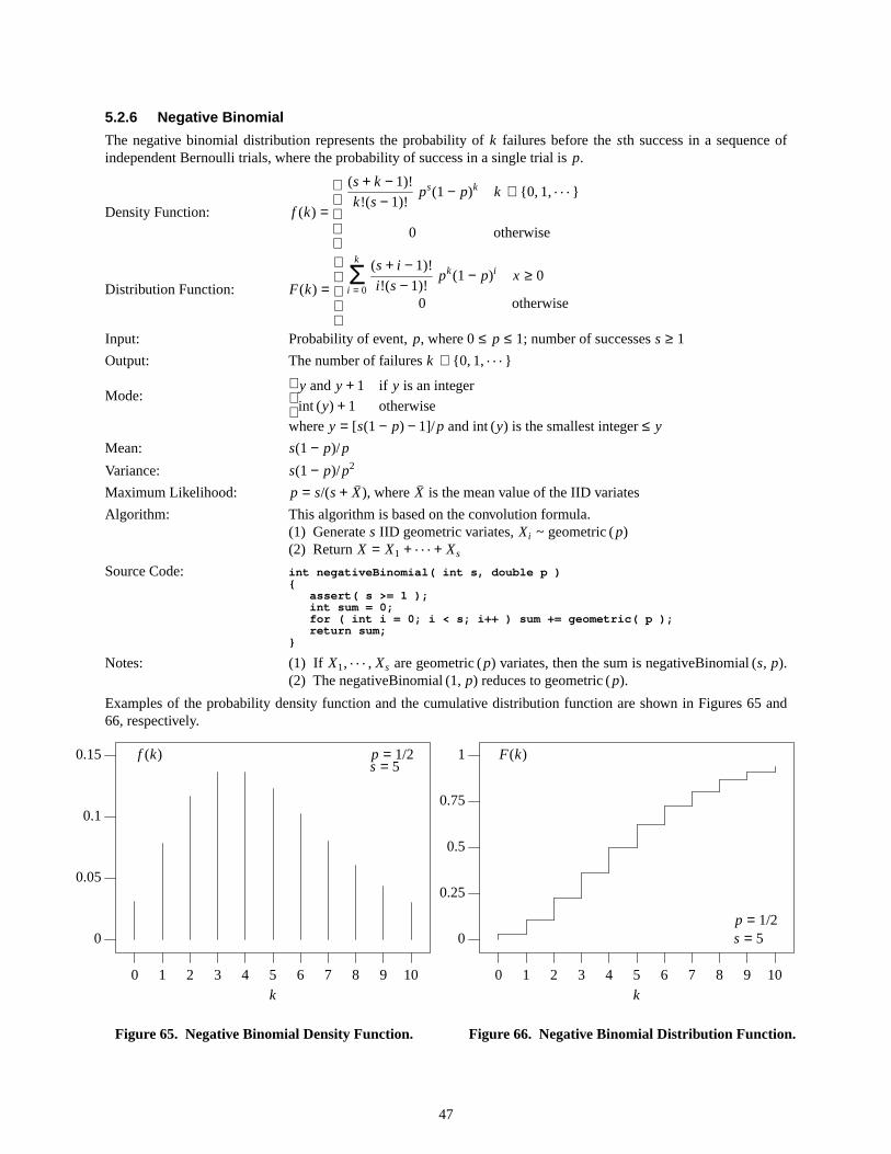
5.2.6 Negative Binomial
The negative binomial distribution represents the probability of k failures before the sth success in a sequence ofindependent Bernoulli trials, where the probability of success in a single trial isp.
Density Function: f (k) =
(s+ k − 1)!
k!(s− 1)!ps(1 − p)k
0
k ∈ { 0, 1, . . . }
otherwise
Distribution Function: F(k) =
k
i = 0Σ (s+ i − 1)!
i !(s− 1)!pk(1 − p)i
0
x ≥ 0
otherwise
Input: Probability of event, p, where 0≤ p ≤ 1; number of successess ≥ 1
Output: Thenumber of failuresk ∈ { 0, 1, . . . }
Mode:
y andy + 1
int (y) + 1
if y is an integer
otherwisewherey = [s(1 − p) − 1]/p and int(y) is the smallest integer≤ y
Mean: s(1 − p)/p
Variance: s(1 − p)/p2
Maximum Likelihood: p = s/(s+ X), whereX is the mean value of the IID variates
Algorithm: This algorithm is based on the convolution formula.(1) Generate s IID geometric variates,Xi ~ geometric (p)(2) Return X = X1 + . . . + Xs
Source Code: int negativeBinomial( int s, double p ){
assert( s >= 1 );int sum = 0;for ( int i = 0; i < s; i++ ) sum += geometric( p );return sum;
}
Notes: (1) If X1, . . . , Xs are geometric (p) variates, then the sum is negativeBinomial (s, p).(2) ThenegativeBinomial (1, p) reduces to geometric(p).
Examples of the probability density function and the cumulative distribution function are shown in Figures 65 and66, respectively.
0
0.05
0.1
0.15
0 1 2 3 4 5 6 7 8 9 10
f (k) p = 1/2s = 5
k
Figure65. Negative Binomial Density Function.
0
0.25
0.5
0.75
1
0 1 2 3 4 5 6 7 8 9 10
F(k)
p = 1/2s = 5
k
Figure66. Negative Binomial Distrib ution Function.
47

5.2.7 Pascal
The Pascal distribution represents the probability of having to perform k trials in order to achieve s successes in asequence ofn independent Bernoulli trials, where the probability of success in a single trial isp.
Density Function: f (k) =
(k − 1)!
(k − s)!(s− 1)!ps(1 − p)k−s
0
k ∈ { s, s+ 1,. . . }
otherwise
Distribution Function: F(k) =
k
i = 1Σ (k − 1)!
(i − s)!(s− 1)!ps(1 − p)i−s
0
k ≥ s
otherwise
Input: Probability of event, p, where 0≤ p ≤ 1; number of successes,s ≥ 1
Output Thenumber of trialsk ∈ { s, s+ 1,. . . }
Mode: The integern that satisfies 1+ np ≥ s ≥ 1 + (n − 1)p
Mean s/p
Variance s(1 − p)/p2
Maximum Likelihood: p = s/n, wheren is the number of trials [unbiassed estimate is (s− 1)/(n − 1)]
Algorithm: This algorithm takes advantage of the logical relationship to the negative binomial.ReturnX = negativeBinomial (s, p) + s
Source Code: int pascal( int s, double p ){
return negativeBinomial( s, p, ) + s;}
Notes: (1) ThePascal and binomial are inverses of each other in that the binomial returnsthe number of successes in a given number of trials, whereas the Pascal returnsthe number of trials required for a given number of successes.
(2) Pascal (s, p) = negativeBinomial (s, p) + s.(3) Pascal (p, 1) = geometric (p) + 1.
Examples of the probability density function and the cumulative distribution function are shown in Figures 67 and68, respectively.
0
0.1
0.2
3 4 5 6 7 8 9 10 11 12 13 14 15
f (x) p = 1/2s = 3
k
Figure67. Pascal Density Function.
0
0.25
0.5
0.75
1
3 4 5 6 7 8 9 10 11 12 13 14 15
F(x)
p = 1/2s = 3
k
Figure68. Pascal Distribution Function.
48
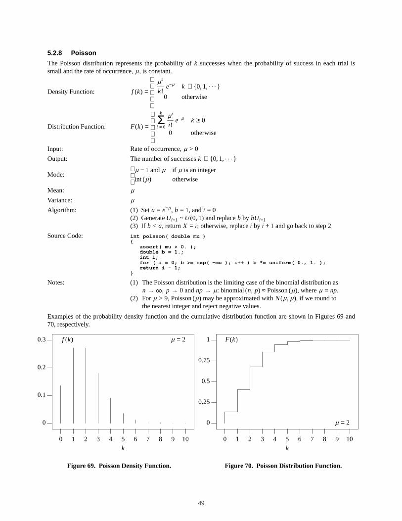
5.2.8 Poisson
The Poisson distribution represents the probability of k successes when the probability of success in each trial issmall and the rate of occurrence,µ, is constant.
Density Function: f (k) =
µk
k!e−µ
0
k ∈ { 0, 1, . . . }
otherwise
Distribution Function: F(k) =
k
i = 0Σ µ i
i !e−µ
0
k ≥ 0
otherwise
Input: Rateof occurrence,µ > 0
Output: Thenumber of successesk ∈ { 0, 1, . . . }
Mode:
µ − 1 and µint (µ)
if µ is an integer
otherwise
Mean: µVariance: µAlgorithm: (1) Set a = e−µ , b = 1, andi = 0
(2) GenerateUi+1 ~ U(0, 1) and replaceb by bUi+1
(3) If b < a, returnX = i ; otherwise, replacei by i + 1 and go back to step 2
Source Code: int poisson( double mu ){
assert( mu > 0. );double b = 1.;int i;for ( i = 0; b >= exp( -mu ); i++ ) b *= uniform( 0., 1. );return i - 1;
}
Notes: (1) ThePoisson distribution is the limiting case of the binomial distribution asn → ∞, p → 0 and np → µ: binomial (n, p) ≈ Poisson (µ), whereµ = np.
(2) For µ > 9, Poisson (µ) may be approximated withN(µ, µ), if we round tothe nearest integer and reject negative values.
Examples of the probability density function and the cumulative distribution function are shown in Figures 69 and70, respectively.
0
0.1
0.2
0.3
0 1 2 3 4 5 6 7 8 9 10
f (k) µ = 2
k
Figure69. Poisson Density Function.
0
0.25
0.5
0.75
1
0 1 2 3 4 5 6 7 8 9 10
F(k)
µ = 2
k
Figure70. Poisson Distribution Function.
49
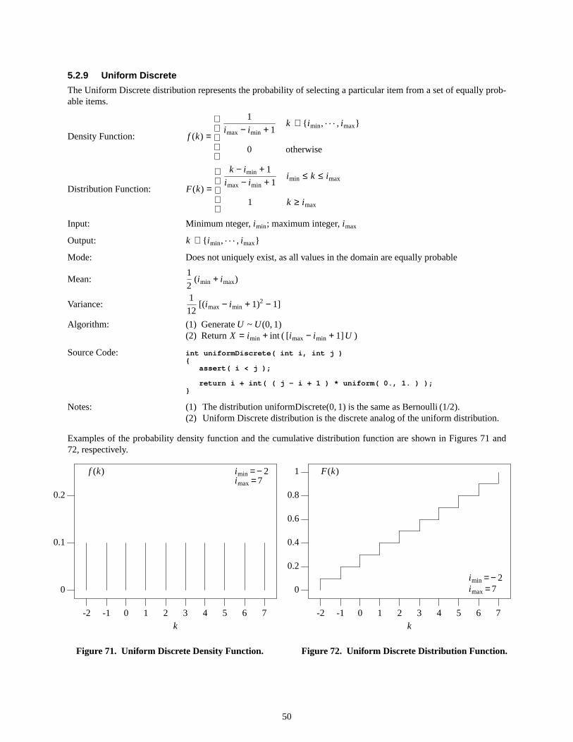
5.2.9 Uniform Discrete
The Uniform Discrete distribution represents the probability of selecting a particular item from a set of equally prob-able items.
Density Function: f (k) =
1
imax − imin + 1
0
k ∈ { imin, . . . , imax}
otherwise
Distribution Function: F(k) =
k − imin + 1
imax − imin + 1
1
imin ≤ k ≤ imax
k ≥ imax
Input: Minimum nteger, imin; maximum integer, imax
Output: k ∈ { imin, . . . , imax}
Mode: Does not uniquely exist, as all values in the domain are equally probable
Mean:1
2(imin + imax)
Variance:1
12[(imax − imin + 1)2 − 1]
Algorithm: (1) GenerateU ~ U(0, 1)(2) Return X = imin + int ( [imax − imin + 1]U )
Source Code: int uniformDiscrete( int i, int j ){
assert( i < j );
return i + int( ( j - i + 1 ) * uniform( 0., 1. ) );}
Notes: (1) Thedistribution uniformDiscrete(0,1) is the same as Bernoulli(1/2).(2) Uniform Discrete distribution is the discrete analog of the uniform distribution.
Examples of the probability density function and the cumulative distribution function are shown in Figures 71 and72, respectively.
k
-2 -1 0 1 2 3 4 5 6 7
0
0.1
0.2
imin =− 2imax=7
f (k)
Figure71. Uniform Discrete Density Function.
k
-2 -1 0 1 2 3 4 5 6 7
0
0.2
0.4
0.6
0.8
1
imin =− 2imax=7
F(k)
Figure72. Uniform Discrete Distribution Function.
50
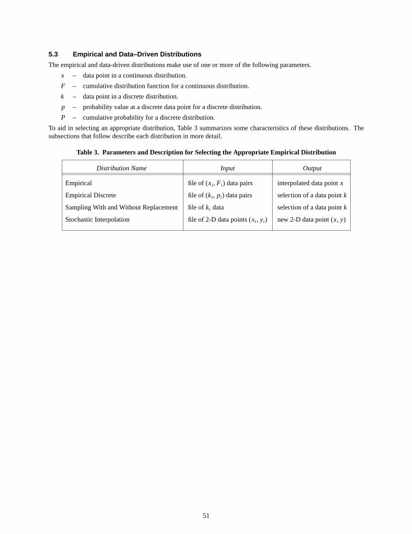
5.3 Empirical and Data–Driven Distrib utions
The empirical and data-driven distributions makeuse of one or more of the following parameters.
x – data point in a continuous distribution.
F – cumulative distribution function for a continuous distribution.
k – data point in a discrete distribution.
p – probability value at a discrete data point for a discrete distribution.
P – cumulative probability for a discrete distribution.
To aid in selecting an appropriate distribution, Table 3 summarizes some characteristics of these distributions. Thesubsections that follow describe each distribution in more detail.
Table 3. Parameters and Description for Selecting the Appropriate Empirical Distrib ution
Distribution Name Input Output
Empirical fileof (xi , Fi ) data pairs interpolated data pointx
Empirical Discrete file of (ki , pi ) data pairs selection of a data pointk
Sampling With and Without Replacement file of ki data selection of a data pointk
Stochastic Interpolation file of 2-D data points (xi , yi ) new 2-D data point (x, y)
51
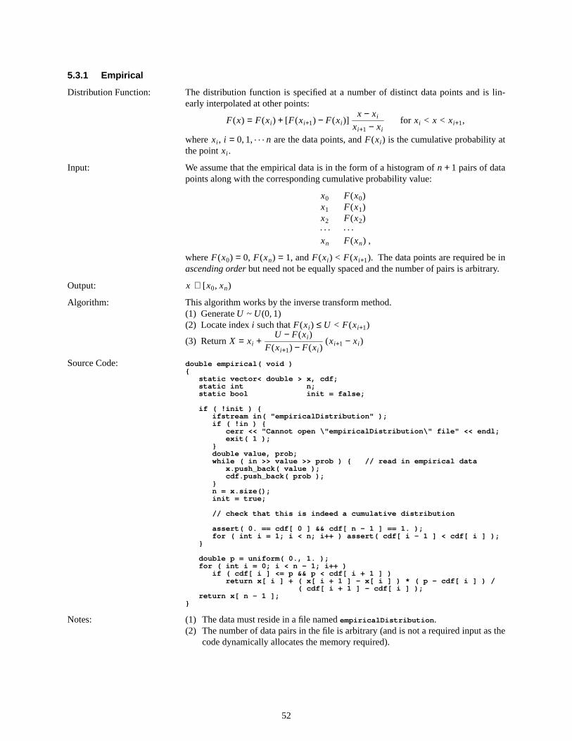
5.3.1 Empirical
Distribution Function: The distribution function is specified at a number of distinct data points and is lin-early interpolated at other points:
F(x) = F(xi ) + [F(xi+1) − F(xi )]x − xi
xi+1 − xifor xi < x < xi+1,
wherexi , i = 0, 1, . . . n are the data points, and F(xi ) is the cumulative probability atthe pointxi .
Input: We assume that the empirical data is in the form of a histogram of n + 1 pairs of datapoints along with the corresponding cumulative probability value:
x0 F(x0)x1 F(x1)x2 F(x2). . . . . .
xn F(xn) ,
whereF(x0) = 0, F(xn) = 1, and F(xi ) < F(xi+1). The data points are required be inascending orderbut need not be equally spaced and the number of pairs is arbitrary.
Output: x ∈ [x0, xn)
Algorithm: This algorithm works by the inverse transform method.(1) GenerateU ~ U(0, 1)(2) Locate index i such thatF(xi ) ≤ U < F(xi+1)
(3) Return X = xi +U − F(xi )
F(xi+1) − F(xi )(xi+1 − xi )
Source Code: double empirical( void ){
static vector< double > x, cdf;static int n;static bool init = false;
if ( !init ) {ifstream in( "empiricalDistribution" );if ( !in ) {
cerr << "Cannot open \"empiricalDistribution\" file" << endl;exit( 1 );
}double value, prob;while ( in >> value >> prob ) { // read in empirical data
x.push_back( value );cdf.push_back( prob );
}n = x.size();init = true;
// check that this is indeed a cumulative distribution
assert( 0. == cdf[ 0 ] && cdf[ n - 1 ] == 1. );for ( int i = 1; i < n; i++ ) assert( cdf[ i - 1 ] < cdf[ i ] );
}
double p = uniform( 0., 1. );for ( int i = 0; i < n - 1; i++ )
if ( cdf[ i ] <= p && p < cdf[ i + 1 ] )return x[ i ] + ( x[ i + 1 ] - x[ i ] ) * ( p - cdf[ i ] ) /
( cdf[ i + 1 ] - cdf[ i ] );return x[ n - 1 ];
}
Notes: (1) Thedata must reside in a file namedempiricalDistribution .(2) The number of data pairs in the file is arbitrary (and is not a required input as the
code dynamically allocates the memory required).
52
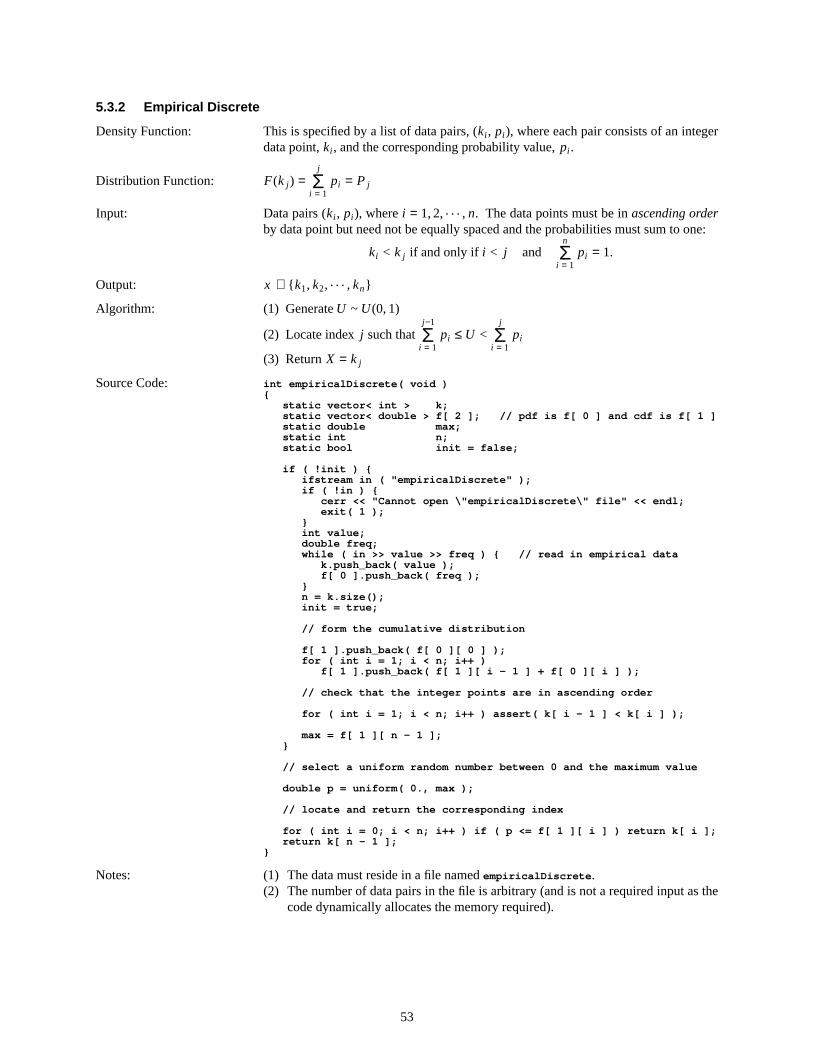
5.3.2 Empirical Discrete
Density Function: This is specified by a list of data pairs, (ki , pi ), where each pair consists of an integerdata point,ki , and the corresponding probability value,pi .
Distribution Function: F(k j ) =j
i = 1Σ pi = Pj
Input: Data pairs (ki , pi ), where i = 1, 2, . . . , n. The data points must be in ascending orderby data point but need not be equally spaced and the probabilities must sum to one:
ki < k j if and only if i < j andn
i = 1Σ pi = 1.
Output: x ∈ { k1, k2, . . . , kn}
Algorithm: (1) GenerateU ~ U(0, 1)
(2) Locate index j such thatj−1
i = 1Σ pi ≤ U <
j
i = 1Σ pi
(3) Return X = k j
Source Code: int empiricalDiscrete( void ){
static vector< int > k;static vector< double > f[ 2 ]; // pdf is f[ 0 ] and cdf is f[ 1 ]static double max;static int n;static bool init = false;
if ( !init ) {ifstream in ( "empiricalDiscrete" );if ( !in ) {
cerr << "Cannot open \"empiricalDiscrete\" file" << endl;exit( 1 );
}int value;double freq;while ( in >> value >> freq ) { // read in empirical data
k.push_back( value );f[ 0 ].push_back( freq );
}n = k.size();init = true;
// form the cumulative distribution
f[ 1 ].push_back( f[ 0 ][ 0 ] );for ( int i = 1; i < n; i++ )
f[ 1 ].push_back( f[ 1 ][ i - 1 ] + f[ 0 ][ i ] );
// check that the integer points are in ascending order
for ( int i = 1; i < n; i++ ) assert( k[ i - 1 ] < k[ i ] );
max = f[ 1 ][ n - 1 ];}
// select a uniform random number between 0 and the maximum value
double p = uniform( 0., max );
// locate and return the corresponding index
for ( int i = 0; i < n; i++ ) if ( p <= f[ 1 ][ i ] ) return k[ i ];return k[ n - 1 ];
}
Notes: (1) Thedata must reside in a file namedempiricalDiscrete .(2) The number of data pairs in the file is arbitrary (and is not a required input as the
code dynamically allocates the memory required).
53
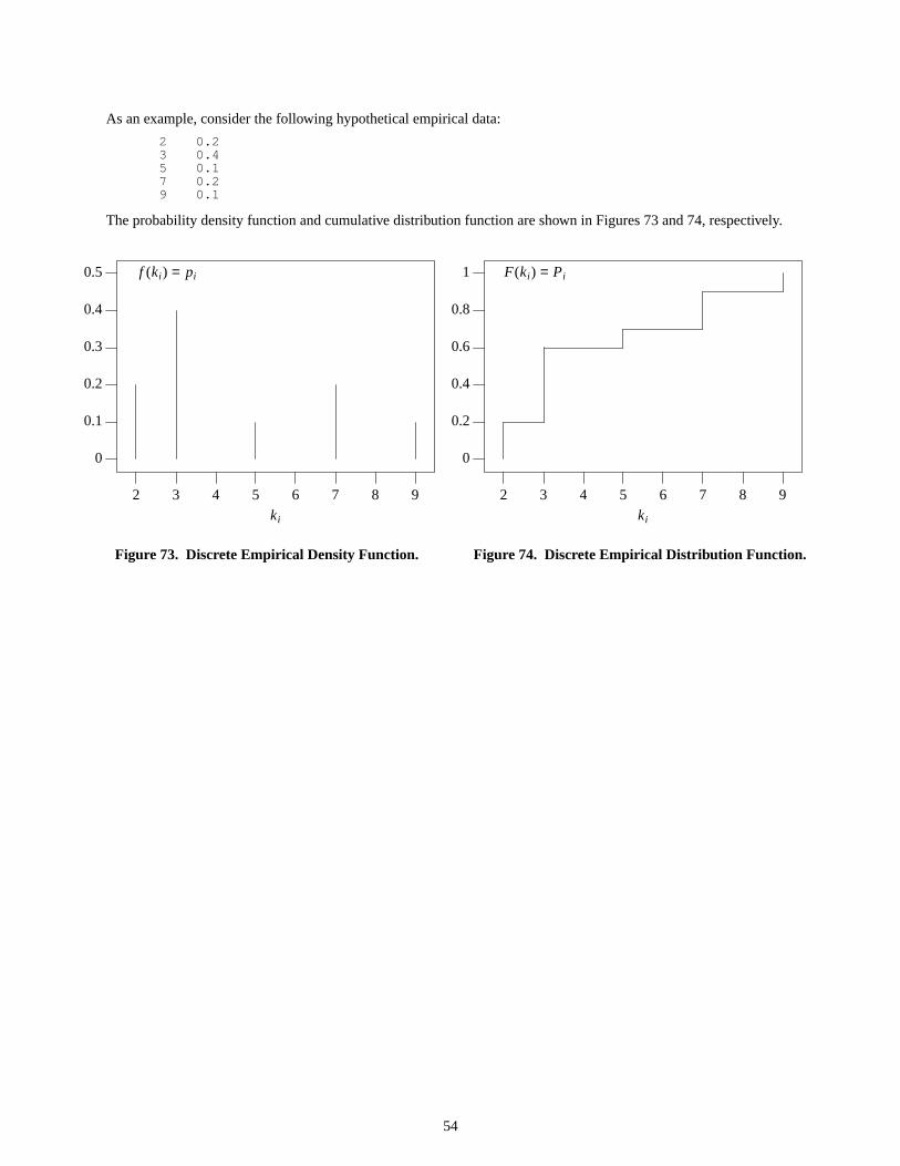
As an example, consider the following hypothetical empirical data:
2 0.23 0.45 0.17 0.29 0.1
The probability density function and cumulative distribution function are shown in Figures 73 and 74, respectively.
ki
2 3 4 5 6 7 8 9
0
0.1
0.2
0.3
0.4
0.5 f (ki ) = pi
Figure73. Discrete Empirical Density Function.
ki
2 3 4 5 6 7 8 9
0
0.2
0.4
0.6
0.8
1 F(ki ) = Pi
Figure74. Discrete Empirical Distribution Function.
54
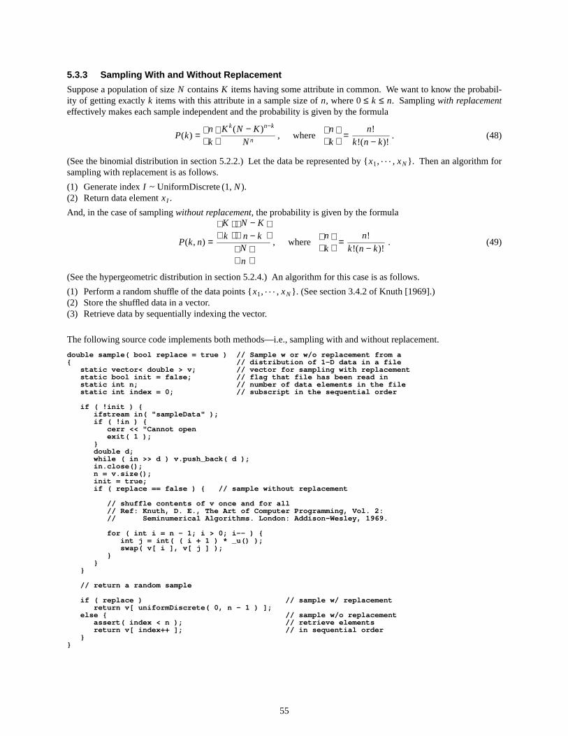
5.3.3 Sampling With and Without Replacement
Suppose a population of size N containsK items having some attribute in common. We want to know the probabil-ity of getting exactly k items with this attribute in a sample size of n, where 0 ≤ k ≤ n. Samplingwith replacementeffectively makes each sample independent and the probability is given by the formula
P(k) =
n
k
K k(N − K )n−k
Nn, where
n
k
=n!
k!(n − k)!. (48)
(See the binomial distribution in section 5.2.2.) Let the data be represented by { x1, . . . , xN} . Then an algorithm forsampling with replacement is as follows.
(1) Generate index I ~ UniformDiscrete (1, N).(2) Return data elementxI .
And, in the case of samplingwithout replacement, the probability is given by the formula
P(k, n) =
K
k
N − K
n − k
N
n
, where
n
k
=n!
k!(n − k)!. (49)
(See the hypergeometric distribution in section 5.2.4.)An algorithm for this case is as follows.
(1) Perform a random shuffle of the data points {x1, . . . , xN}. (See section 3.4.2 of Knuth [1969].)(2) Store the shuffled data in a vector.(3) Retrieve data by sequentially indexing the vector.
The following source code implements both methods—i.e., sampling with and without replacement.
double sample( bool replace = true ) // Sample w or w/o replacement from a{ / / distribution of 1-D data in a file
static vector< double > v; // vector for sampling with replacementstatic bool init = false; // flag that file has been read instatic int n; // number of data elements in the filestatic int index = 0; // subscript in the sequential order
if ( !init ) {ifstream in( "sampleData" );if ( !in ) {
cerr << "Cannot openexit( 1 );
}double d;while ( in >> d ) v.push_back( d );in.close();n = v.size();init = true;if ( replace == false ) { // sample without replacement
// shuffle contents of v once and for all// Ref: Knuth, D. E., The Art of Computer Programming, Vol. 2:/ / Semi numer i cal Algorithms. London: Addison-Wesley, 1969.
for ( int i = n - 1; i > 0; i-- ) {int j = int( ( i + 1 ) * _u() );swap( v[ i ], v[ j ] );
}}
}
// return a random sample
if ( replace ) // sample w/ replacementreturn v[ uniformDiscrete( 0, n - 1 ) ];
else { // sample w/o replacementassert( index < n ); // retrieve elementsreturn v[ index++ ]; // in sequential order
}}
55

5.3.4 Stochastic Interpolation
Sampling (with or without replacement) can only return some combination of the original data points. Stochasticinterpolation is a more sophisticated technique that will generate new data points. It is designed to give the new datathe same local statistical properties as the original data and is based on the following algorithm.
(1) Translate and scale multivariate data so that each dimension has the same range:x ⇒ (x − xmin)/|xmax − xmin|.
(2) Randomly select (with replacement) one of the n data points along with its nearest m − 1 neighborsx1, . . . , xm−1
and compute the sample mean:
x =1
m
m
i =1Σ xi .
(3) Generate m IID uniform variates
Ui ~ U
1 − √ 3(m − 1)
m,1 + √ 3(m − 1)
m
and set
X = x +m
i =1Σ (xi − x)Ui .
(4) RescaleX by (xmax − xmin) and shift toxmin.
The following source code implements stochastic interpolation.
// comparison functor for use in determining the neighborhood of a data point
struct dSquared : public binary_function< point, point, bool > {bool operator()( point p, point q ) {
return p.x * p.x + p.y * p.y < q.x * q.x + q.y * q.y;}
};
point stochasticInterpolation( void )
// Refs: Taylor, M. S. and J. R. Thompson, Computational Statistics & Data/ / Anal ysi s, Vol. 4, pp. 93-101, 1986; Thompson, J. R., Empirical Model/ / Bui l di ng, pp. 108-114, Wiley, 1989; Bodt, B. A. and M. S. Taylor,/ / A Data Based Random Number Generator for A Multivariate Distribution -/ / A User’s Manual, ARBRL-TR-02439, BRL, APG, MD, Nov. 1982.{
static vector< point > data;static point min, max;static int m;static double lower, upper;static bool init = false;
if ( !init ) {ifstream in( "stochasticData" );if ( !in ) {
cerr << "Cannot open \"stochasticData\" input file" << endl;exit( 1 );
}
// read in the data and set min and max values
min.x = min.y = FLT_MAX;max.x = max.y = FLT_MIN;point p;while ( in >> p.x >> p.y ) {
min.x = ( p.x < min.x ? p.x : min.x );min.y = ( p.y < min.y ? p.y : min.y );max.x = ( p.x > max.x ? p.x : max.x );max.y = ( p.y > max.y ? p.y : max.y );
data.push_back( p );}in.close();init = true;
56
// scale the data so that each dimension will have equal weight
for ( int i = 0; i < data.size(); i++ ) {
data[ i ].x = ( data[ i ].x - min.x ) / ( max.x - min.x );data[ i ].y = ( data[ i ].y - min.y ) / ( max.y - min.y );
}
// set m, the number of points in a neighborhood of a given point
m = data.size() / 20; // 5% of all the data pointsif ( m < 5 ) m = 5; / / but no less than 5if ( m > 20 ) m = 20; // and no more than 20
lower = ( 1. - sqrt( 3. * ( double( m ) - 1. ) ) ) / double( m );upper = ( 1. + sqrt( 3. * ( double( m ) - 1. ) ) ) / double( m );
}
// uniform random selection of a data point (with replacement)
point origin = data[ uniformInt( 0, data.size() - 1 ) ];
// make this point the origin of the coordinate system
for ( int n = 0; n < data.size(); n++ ) data[ n ] -= origin;
// sort the data with respect to its distance (squared) from this origin
sort( data.begin(), data.end(), dSquared() );
// find the mean value of the data in the neighborhood about this point
point mean;mean.x = mean.y = 0.;for ( int n = 0; n < m; n++ ) mean += data[ n ];mean /= double( m );
// select a random linear combination of the points in this neighborhood
point p;p.x = p.y = 0.;for ( int n = 0; n < m; n++ ) {
double rn;if ( m == 1 ) rn = 1.;el se r n = uniform( lower, upper );
p.x += rn * ( data[ n ].x - mean.x );p.y += rn * ( data[ n ].y - mean.y );
}
// restore the data to its original form
for ( int n = 0; n < data.size(); n++ ) data[ n ] += origin;
// use the mean and the original point to translate the randomly-chosen point
p += mean;p += origin;
// scale the randomly-chosen point to the dimensions of the original data
p.x = p.x * ( max.x - min.x ) + min.x;p.y = p.y * ( max.y - min.y ) + min.y;
return p;}
Notes: (1) Notice that with the particular range on the uniform distribution in step 3 of the algorithm ischosen to give a mean value of 1/m and a variance of (m − 1)/m2.
(2) When m = 1, this reduces to the bootstrap method of sampling with replacement.
57
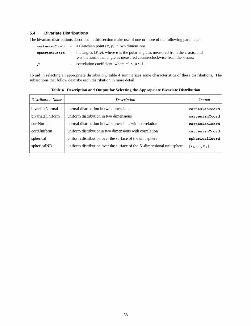
5.4 Bivariate Distrib utions
The bivariate distributions described in this section makeuse of one or more of the following parameters.
cartesianCoord – aCartesian point (x, y) in two dimensions.
sphericalCoord – the angles (θ ,φ), whereθ is the polar angle as measured from thez-axis, andφ is the azimuthal angle as measured counterclockwise from thex-axis.
ρ – correlation coefficient, where−1 ≤ ρ ≤ 1.
To aid in selecting an appropriate distribution, Table 4 summarizes some characteristics of these distributions. Thesubsections that follow describe each distribution in more detail.
Table 4. Description and Output for Selecting the Appropriate Bivariate Distrib ution
Distribution Name Description Output
bivariateNormal normal distribution in two dimensions cartesianCoord
bivariateUniform uniform distribution in two dimensions cartesianCoord
corrNormal normal distribution in two dimensions with correlation cartesianCoord
corrUniform uniform distributionin two dimensions with correlation cartesianCoord
spherical uniform distribution over the surface of the unit sphere sphericalCoord
sphericalND uniform distribution over the surface of theN-dimensional unit sphere (x1, . . . , xN)
58
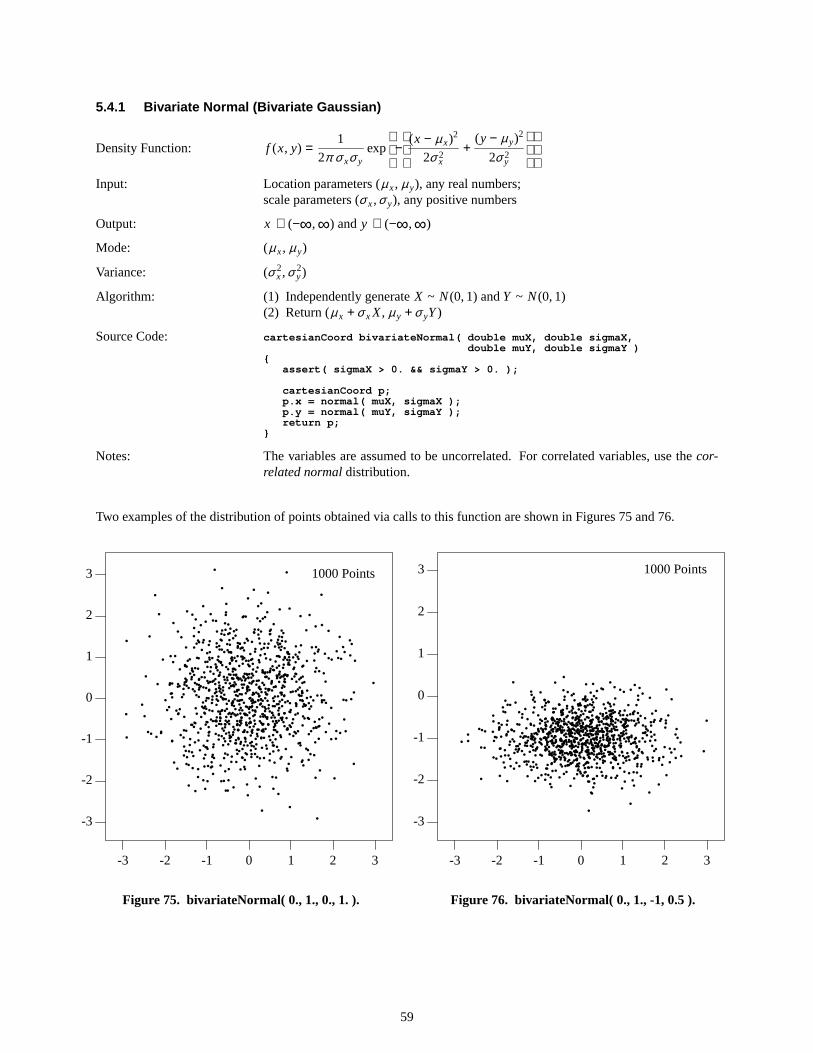
5.4.1 Bivariate Normal (Biv ariate Gaussian)
Density Function: f (x, y) =1
2π σ xσ yexp
−
(x − µ x)2
2σ 2x
+(y − µ y)
2
2σ 2y
Input: Location parameters (µ x, µ y), any real numbers;scale parameters (σ x,σ y), any positive numbers
Output: x ∈ (−∞,∞) and y ∈ (−∞,∞)
Mode: (µ x, µ y)
Variance: (σ 2x,σ 2
y)
Algorithm: (1) Independently generateX ~ N(0, 1) andY ~ N(0, 1)(2) Return (µ x + σ x X, µ y + σ yY)
Source Code: cartesianCoord bivariateNormal( double muX, double sigmaX,double muY, double sigmaY )
{assert( sigmaX > 0. && sigmaY > 0. );
cartesianCoord p;p.x = normal( muX, sigmaX );p.y = normal( muY, sigmaY );return p;
}
Notes: The variables are assumed to be uncorrelated. For correlated variables, use the cor-related normaldistribution.
Tw o examples of the distribution of points obtained via calls to this function are shown in Figures 75 and 76.
•• •
• •• ••• •• •• ••• ••• • ••••• • • • ••• • •• •• • •••• •• ••• •••• • •• •••• ••• ••• •••• ••• •• ••• ••• • •• ••• •• •• •• •• ••• •• •• •• •••• •• •• ••• •• • •• ••• • • ••• •• • •• •• ••••• ••• • • •• • •• • • • • •• •• • • •••• •••• ••• •• •• • ••• • ••• •• • •• ••• • •• • ••• • •• ••• • •• •• • •• •• ••• •••• ••• •• • ••• • • ••••• •••• • •• • •• • • •• ••• •• • ••• • •••• • •••• • •• •• ••• • ••• • •• ••• •• •••• •• • • •• ••• •• •••• •• • ••• •• •• •••• ••• ••• •• • •• •• •• • •• •• • ••• •• •• • •• •••• • • •• ••• ••• •• ••••• ••• ••• • •• •• •• • •• •• •••• •• ••• • •• • ••• ••• • • • •• •• • •• •••••• •• •• ••• • ••• ••• •••• •• •• •• •• •••• •• •• • • • • •• •• • •• •• ••• ••• • •••• ••• •• •• • •• • •• • •• •• •• • •• • ••••• ••• •••• •• •••• •• ••• • ••• •• ••• • •••• • •• •• • ••• ••• •• ••• • • ••• • •••• • •• ••• •• • •• • ••• •• ••• ••• • •• ••• • • ••••• • • •• ••• • ••• •••• • • • ••• ••• •• ••••• •• ••••• • • • •• • •• •• ••• ••• •••• •••• • •••• •• ••• • ••• ••• ••• ••• •••• • •• •• ••• ••••• • ••• • ••• ••••• • •• •• •• ••• • • ••• •• • ••• •••• ••• • ••• •• • •• ••• ••• • ••• ••• •• ••••• •• •• ••• •• • ••• ••• •••• •• ••• • •• •• • • •• •• ••• • ••• • • •••• • •• •• ••• • •• ••• • •••• • •• •• • • •• • • •••• •• •• ••• ••••••• •• ••• ••• ••• •• • •• •••• ••• •• • • ••• • ••• •• •• • ••• •• • ••• • ••• • •• • •••• • ••••• • •• • ••• •• • • •••• •• •• ••• • •••• ••• ••• •• ••• • • •• • •• •• ••• ••••
••
-3 -2 -1 0 1 2 3
-3
-2
-1
0
1
2
3 1000 Points
Figure75. bivariateNormal( 0., 1., 0., 1. ).
•
•
•
•
••
••
•
•
• •
••
•
••
•
••
•
• •
•
•
•
••
•
•
•
••
•
•
•
• •
••
•
• •
•
•
•
•
•
•
•
••
•
•
•
••
•
•
••
••
••
•
•
•
••
•
••
•
• •
•
•
•
••
•
•
•
• •
•
•
••
•
•
•
• •••
•
•• •
•
••
•
•
•
••
•••
•
•
•
••
••
•
•
•
•
•
• •
•
•
•
••
•••
••
••
•
•
••
•
•
• •
•
••
•
••
• ••
•
••
•
•
••
•
•
••
••••
••
•
•
•
•
•
•• •
•
•
•
•
•
••
••• •
•
•
••
•
•
••
• • •
•
•
•• •
••
•
•• •
•
•
••
••
• •
•
•
•
•
••••
•
• ••
•
••
•
• •
•
•
••
•
•
••
•
•
•
• •
•
••
•
•• •••
•
•
•
•
••
••
•
••
••
•
•
••
•
•
•
•••
••••
•
••
•
•
••
••
• ••
••
• •
•
•
•
••
•
•
••
•
••
•
•
•
•
•
••
•
•
•
•
•
•
•
•
•
••
••
•
• •
•
•
•••
•
• •
•
•
••
•
• •
•
•••
•
•
•
•
•
••
••
•
•
•
•
•
•
•
•
••
•
•
• ••
•
•
••
•
•
••
• •
••
• ••
•
•
•
••
•
•
••
•
••
•
•
••
••
••
••
•
•
•
•
•
••
•
•
••• ••
•
•••
•
•
•
••
•
••
•
•
•• •
•
• •
•• •••
•
•
••
•
•
• •
•
•
•
•
•
•
•••
•
••
• ••
•
•
•
•
•
•
•
••
••
•
•
••
••
••
••
•
•
•
•
•
••
••
• •
•
•
• ••
•
•
•
•
•
•
•••
•
•
••
•
•
•
•
•
•••
•
••
•
••
•
•
•
•
• ••
•
•
••
••
•
•
••
•
•
•
•
•
•
•
•
•
•
•
••
••
••
•
•
•
•• •
• ••
••
•
••
•
•
•
••
•
•
••
• ••••
•
••
•
• •••
•
•
••
•
•
•
•
•
•• •
•
• •
• •
••
•
••
•••
•
•
••
•• ••
•
•
•
•
••
•
•
•••
•
•
•
•
•
••
••
•
• •
•
•
•
•
•
••
•
••
•
••
•
•
•
••
•••
•
••
••
••
•
•
• ••
•
•
•
•
•
•
••
••
• ••
•
•
•
•
•
•
•••
•
••
•
••
•
•
••• •
•
•
•
•
••
•••
•
•• ••
•
• •
• • •• •• •• •
•
•
•
•
•
•
•
•
•
•
•
•
•
••
••
••
••
•
•
••
••
•
•
•• •
•
••
••
•
•
•
•
••
•••
••
•
•
•••
••
••••
•
•• •
•
•
•
•
•
•
•
••
••
••
••
•
•••
••
•
••
••
•••
•••
•••
••
•
•
•
•
•
•
• •••
•
•
•
• •
• ••
•
•
• •
•
• •
••
•
••
•
•
•
•
••
•
•
••
•
••
•
•
•
••
•
• •
•
••
••
••
•
•
•• •
•
•
••
•••
•
•
••••
•
•••
•
•
•
••
•
•
•
•
•••
•
•
••
• •
•
••
•
•
•
••
•
•
•
•
•
•
•
•
•
•
•• •• •
•
•• ••
••
••
•
•
•
•••
-3 -2 -1 0 1 2 3
-3
-2
-1
0
1
2
3 1000 Points
Figure76. bivariateNormal( 0., 1., -1, 0.5 ).
59
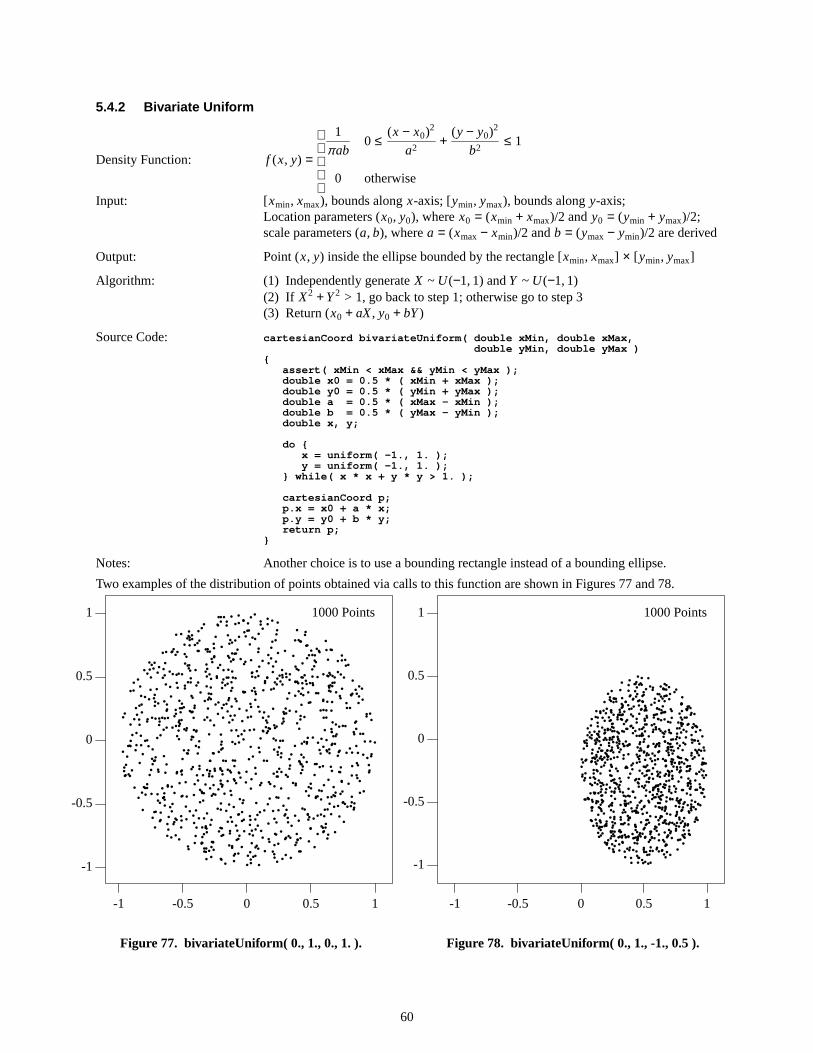
5.4.2 Bivariate Unif orm
Density Function: f (x, y) =
1
πab
0
0 ≤(x − x0)2
a2+
(y − y0)2
b2≤ 1
otherwise
Input: [xmin, xmax), bounds alongx-axis; [ymin, ymax), bounds alongy-axis;Location parameters (x0, y0), wherex0 = (xmin + xmax)/2 andy0 = (ymin + ymax)/2;scale parameters (a, b), wherea = (xmax − xmin)/2 andb = (ymax − ymin)/2 are derived
Output: Point (x, y) inside the ellipse bounded by the rectangle [xmin, xmax] × [ymin, ymax]
Algorithm: (1) Independently generateX ~ U(−1, 1) andY ~ U(−1, 1)(2) If X2 + Y2 > 1, go back to step 1; otherwise go to step 3(3) Return (x0 + aX, y0 + bY)
Source Code: cartesianCoord bivariateUniform( double xMin, double xMax,double yMin, double yMax )
{assert( xMin < xMax && yMin < yMax );double x0 = 0.5 * ( xMin + xMax );double y0 = 0.5 * ( yMin + yMax );double a = 0.5 * ( xMax - xMin );double b = 0.5 * ( yMax - yMin );double x, y;
do {x = uniform( -1., 1. );y = uniform( -1., 1. );
} while( x * x + y * y > 1. );
cartesianCoord p;p.x = x0 + a * x;p.y = y0 + b * y;return p;
}
Notes: Another choice is to use a bounding rectangle instead of a bounding ellipse.
Tw o examples of the distribution of points obtained via calls to this function are shown in Figures 77 and 78.
-1 -0.5 0 0.5 1
-1
-0.5
0
0.5
1
•
•
•
•
•
•
•
•
•
• •
•
•
•
•
••
•
••
•
•
•
• •
•
•
•
•
•
•
•
•
•
•
•
•
•
•
•
•
•
•
•
•
•
•
••
•
•
•
•
•
•
•
•
••
• •
•
•
•
•
•
•
• ••
•
•
•
•
•
•
•
•
•
•
•
•
••
•
•
•
•
•
•
•
•
•
•
•
•
•
••
•
•
•
•
••
•
•
••
• •
•
••
•
•
••
•
•
•
•
•
••
•
•
•
••
•
•
•
•
•
•
••
•
•
•
•
•
•
•
•
• •
•
•
•
•
•
•
•
•
•
•
•
•
•
•
•
•
••
• ••
••
••
•
•
•
•
•
•
•
•
•
•
•
•
•
•
•
•
•
•
•
•
•
•
•
•
•
••
•• •
•
•
•
•
•
•
• •
•
•
•
•
•
••
•
•
•
•
•
•
•
•
•
•
•
• ••
•
•
•
•
•
•
•
•
•
•
•
•
•
•
••
•
•
•
•
•
•
•
•
••
•
•
•
•
•
•
•
•
•
••
•
•
•
•
•
•
•
•
•
•
•
•
•
•
•
•
•
•
••
•
•
•
•
•
•
••
•
•
•
•
•
••
•
•
•
••
•
•
•
•
•
•
•
•
•
•
•
•
•
•
•
••
•
•
•
•
•
•
•
•
•
•
•
•
• •
•
•
•
•
•
••
••
•
•
••
•
•
•
•
•
•
•
•
•
••
••
•
••
•
•
•
•
•
•
••
•
•
•
•
•
••
•
•
•
•
•
•
•
•
•
•
•
•
•
•
•
•
•
•
•
••
•
•
•
•
•
•
•
•
••
•
•
•
•
•
••
•
•
•
•
•
•
•
•
•
•
•
•
•
•
•
•
•
•
•
•
•
•
•
•
•
•
•
• •
•
•
•
•
•
•
•
•
•
•
•
•
•
•
•
•
•
•
•
•
•
•••
•
•
•
•
•
•
•
•
•
•••
•
•
•
•
•
•
•
•
•
•
•
••
•
•
•
•
•
•
•
•
•
•
••
•
•
•
• •
••
•
• •
•
•
••
••
•
•
••
•
••
•
•
••
•
•
•
•
•
•
••
•
•
•
•
••
•
•
••
•
•
•
•
•
•
•
•
•
•
•
•
•
•
•
••
•
•
••
•
•
•
••
•
•
••
•
•
•
•
•
•
••
•
•
•
•
•
•
•
•
•
•
•
••
•
••
•
•
•
•
•
•
•
•
•
•
•
•
•
•
•
•
•
•
•
•
•
•
•
•
•
•
•
•
•
•
••
•
•
•
•
••
•
•
•
•
••
••
•
•
•
•
•
•
•
•
•
•
•
•
•
•
•
•
•
•
••
•
•
••
•
•
•
•
•
•
•
•
•
•
•
•
•
•
•
•
•
•
•
•
•
•
•
•
•
•
•
•
•
•
•
•
•
•
•
•
•
•
•
•
•
•
•
•
•
••
•
•
•
•
•
•
•
•
•
•
•
•
•
•
•
•
•
••
••
•
•
••
•
•
•
•
•
••
••
••
•
•
•
•
•
•
•
•
•
•
•
•
•
•
•
•
•
•
•
•
•
•
•
•
•
•
•
•
•
•
•
•
•
•
•
•
•
•
•
••
•
•
••
•
• •
•
•
•
•
•
•
•
••
•
•
•
•
•
•
•
•
•
•
•
•
•
•
•
•
•
•
•
•
•
•
•
•
•
•
•
•
•
•
•
•
••
•
•
••
•
•
•
•
•
•
•
•
•
•
••
•
••
•
•
••
•
•
•
•
••
•
•
•
•
•
•
•
•
•
•
•
•
•
•
•
•
•
•
•
•
•
••
•
•
•
•
•
•
•
•
•
•
•
•
••
•
•
•
•
•
•
•
•
•
••
•
•
•
•
•
•
•
•
•
•
•
•
•••
•
•
•
••
•
•
•
•
•
•
•
•
•
•
•
•
•
•
•
•
•
•
•
•
•
•
•
•
•
•
•
•
••
••
••
•
•
•
•
•
•
•
•
•
•
•
•
•
•
1000 Points
Figure77. bivariateUnif orm( 0., 1., 0., 1. ).
•
•
••
•
•
•
•
••
•
•
••
•
•
•
•
•
• •
•
•
•
•
• •
•
•
•
•
•
•
•
•
•
•
••
•
•
•
•
••
•• •
•
••
••
•
•
•
•
• •
•
•
•
•
•
•
•
•
•
•
•
•
•
•
•
•
•
•
•
•
•
•
•
•
••
••
•
•
•
••
•
•
•
••
•
•
•
•
• •
••
•
•
•
••
•
•
•
•
•
•
•
•
• •
•
•
••
•
•
•
•
•
••
• •
• •••
•
•
•
•
•
•
•
•
•
•
•
•
•
•
•
•••
•
•
•
•
•
•
•
•
•
•
• •
•
•
•
•
•
••
•
••
•
•
•
•
••
•
•
•
•
•
•
•
•
•
•
•
••
•
•
•
•
•
•
••
•
•
•
•
••
•
•
•
•
•
•
•
•
•
•
•
•
•
•
•
•
•
•
•
•
•
•
•
•
•
•
•
•
•
•
•
•
•
•
••
•••
•
•
•
•
••
•
•
•
•
•
•
•
•
•
• •
•
•
•
•
••
•
•
•
••
•
••
•
••
•
•
•
•
•
••
•
•
•
•
•
•
•
•
•
•
•
•
••
•
•
••
•
••
••
•
•
•
•
•
•
•
•
•
•
•
•
•
•
•
•
•
••
•
••
•
•
•
•
••
•
•
•
•
•
•
•
••
•
•
• •
•
•
••
••
•
•
•
•
•
•
•
•
•
••
•
•
•
•
••
•
•
•
••
•
•
•
•
•
•
•
•
•
••
••
•
•
•
•
•
•
•••
•
•
•
•
••
•
•••
•
••
•
•
•••
•
••
•
• •
•
• •
••
•
•
•
•
••
•
•
•
••
•
•
•
•
•
•
••
••
•
•
•
•
•
•
•••
•
•
•
•
•
•
•
•
•
•
•
•
•
•
•
••
•
•
•
•
•
•
• •
••
•
•
•
•
•
•
•
•
•
•
•
•
••
•
•
•
•
•
•
••
•
•
•
•
••
•
•
••
•
•
••
•
•
•
•
•
•
•
•
•
•
••
•
•
•
••
• ••
•
••
•
••
•
•
•
•
•
•
•
•
••
••
•
•
•
•
•
•
•
•
••
•
•
•
•
•
••
•
•
•
•
•••
•
•
•
••
•
•
•
•
•
•
•
•
•
•
• •
•• •
•
•
•
•
••
••• •
••
•
•
•
•
•
•
•
•
•
•
•
•
•
• •
••
•
•
•
•
•
•
•
•
•
•
•••
•
•
•
•
•
•
•
•
•
•
•
•
•
•
•
•
•
••
•
••
•
•
•
•
•
•
••
•
•
•
•
•
•
•
•
•
•
•
•
•
•
• •
•
• •
•
•
••
•
•
•
•
•
•
•
•
•
•
•
••
••
•
•
•
•
•
•
•
••
•
•
•
•
•
•
•
•
•
•
•
•
•
•
•
•
•
•
•
•
•
•
••
•
•
•
•
•
•
•
•
•
••
••
•
•
•
•
•
•
•
••
•
•
•
•
•
•
•
•
• •
•
•
••
•
•
•
•
•
•
••
•
•
•
• •
•
•
••
•
•
•
••
•
•
•
•
•
•
•
•
•
•
• •
•
•
••
•
•
•
•
•
••
•
•
•
•• •
••
•
•
••
•
•
••
•
•
•
••
•
••
•
•• •
•
•
•
••
•
•
•
••
•
•
•
•
•
• •
•
••
•
•
•
•
•
•••
•
••
••
•
•
•
•
•• •
•
•
•
•
•
•
•
••
•
•
•
•
•
•
••
•
• •
•
••
•
•
•
•
•
•
•
•
•
•
•
•
•
•
•
••
•
•
•
•
••
••
•
•
••
•
•
•
•
•
•
•
••
•
•
••
•
•
• •
•
•
•
•
••
•
••
•
••
•
•
•
••
•
•••
•
•
•
•
•
•
•
•
•
•
-1 -0.5 0 0.5 1
-1
-0.5
0
0.5
1 1000 Points
Figure78. bivariateUnif orm( 0., 1., -1., 0.5 ).
60

5.4.3 Correlated Normal
Density Function: f (x, y) =1
2π σ xσ y√ 1 − ρ2exp
−
1
1 − ρ2
(x − µ x)2
2σ 2x
−ρ(x − µ x)(y − µ y)
σ xσ y+
(y − µ y)2
2σ 2y
Input: Location parameters (µ x, µ y), any real numbers; positive scale parameters (σ x,σ y);correlation coefficient,−1 ≤ ρ ≤ 1
Output: Point (x, y), wherex ∈ (−∞,∞) and y ∈ (−∞,∞)
Mode: (µ x, µ y)
Variance: (σ 2x,σ 2
y)
Correlation Coefficient: ρ
Algorithm: (1) Independently generateX ~ N(0, 1) andZ ~ N(0, 1)
(2) Set Y = ρ X + √ 1 − ρ2 Z(3) Return (µ x + σ x X, µ y + σ yY)
Source Code: cartesianCoord corrNormal( double r, double muX, double sigmaX,double muY, double sigmaY )
{assert( -1. <= r && r <= 1. ); // bounds on corr coeffassert( sigmaX > 0. && sigmaY > 0. ); // positive std dev
double x = normal();double y = normal();
y = r * x + sqrt( 1. - r * r ) * y; // correlate the variables
cartesianCoord p;p.x = muX + sigmaX * x; // translate and scalep.y = muY + sigmaY * y;return p;
}
Tw o examples of the distribution of points obtained via calls to this function are shown in Figures 79 and 80.
•• ••• ••• • • ••••• • • • ••••• •••• •• •• •• ••• ••• • •• ••• •• •• ••• • •• ••• ••• •• •• • • •• ••• ••• •• ••••• •• •• • •• ••• •••••• ••• •• • ••• •••• •• •• • • •••• ••• •• •• •• ••• • •••• • ••• •• ••• • ••• •• • ••• ••• •• •• • •• •••• ••• •••• • • ••••• •• ••• •• • ••• ••• •• •• •• • •• • •••• •• • ••• •• ••• • ••• ••• ••• •• •• ••• ••• ••• • • •••• •• • •••• •• • •••• ••••• •• •• •• ••• ••• •• • • ••• • ••••• • • •• •• • ••• •• ••• • • •• ••• ••• • ••• • •• •• ••• ••• ••••• ••• • • ••• •• •• •••• • •• ••• •• • • •• ••• ••• •• • • •• ••• • ••• ••• ••• •• • ••• •• •• ••• •• • •• • • •• ••• •• •• • ••• ••• ••• • •• • ••• • • •• • •••• • •• • • •••• ••• ••• •• •• •••• ••••• ••• • •• •• •• • •••• • • ••• • •• • ••••• ••• • •• • ••• •• • • ••• •••••• • •• • •• ••• • •• •• •••• •• •• •• •• ••• •• ••• •• •• •• ••• •• •• • •• • •• • • • •• •••• •• • •• • •• •• • ••••••• •• •• ••• •• •• • ••• ••• • •••• • •• • •• •• ••• •• ••• •••• ••• • •• •• •• • ••• • •• •••• •• •• • ••• • •• • •• • • •••• •• • ••• •• • •• •• •••• •• ••• • •• •• •• ••• • •••• • • ••• • ••• •• • • ••••• ••• ••• ••• •• •• • •• ••• •• • • •• • • •••• • • ••• •• •• ••• • • ••• •• ••• • •• •• •• ••• ••• •• •• •• •• •• • •••• • •••• • ••• •• •• •• •• • •••• •• • •••• • • •• •• ••• •• ••• •• •• ••••• •• •• •••• • ••• • ••• •• •• • •• • •• •• • •• ••• •• •••• ••• • •••• •• •• •• • ••• •• •• •• ••• ••• ••• •• ••• •• •• •• ••• ••• • •• •• •••• ••• •• • • •• •• •• •
•
1000 Points
ρ = 0. 5
-3 -2 -1 0 1 2 3
-3
-2
-1
0
1
2
3
Figure79. corrNormal( 0.5, 0., 1., 0., 1. ).
••
•
•
•
••
••
•••
•
•
•
••
•
••
•••
•
••
•
•
•
•
••
•
•
•
•
• ••
••
•
•• •
•
••
••
••
• •
•
•
•
•
•
•
••
••
••
•
•
•
••••
• •• •
•
•
••
•
•
•
••
•
••
••
•
••
••
•
••
••
•••
•
•
•
• ••
•••
••
•
•
•
•
•
• •
•
•
••
•
••
•
•
• •
•
••
••
••
•
•
•
••• •
•
••
•
•
• •
••
• •
•
•
•
•
•
•
••
•
•
••• ••
•••
••
•
•
• •
••
•
••
••
•••
•
•
••
•
•
••
•
••
•
•
•
•
•
•
• •
•
•
••
• ••• ••
• •
••
•
•••
•
••
•
•
•• •
•
• ••
•
•
•
••
•
•
•
••
•••
•
•
•
•
•
•••
•
•
••
• •
•
•• •
•
•
••
••
•
•
••
•
•
•
••
•
•
•
••
• •
• ••
•
•
•
•
•
•
•
•
• ••
••
•
••
•
•
•
••
•
•
•
•
••
•
•
•
••
••
•
•
•
•
•
•••
••
••
•
••
•
•
• ••••
•
•
•
•
•
•
•
•
•
•
•
•
••••
•
•
•
•
•
•
•
•
•
•
••
••
•
••
••
••
•
•
•
•• •
•
•
••
•
• •
•
•
•
•
•
•
•
•••
•
••
••
•
•
•
•
•
•
••
••
•
••
••
•
••
•••
•
••
•
••
••
•
• •••
••
•
•
•
•
•
•••
•
•
•
•
•
••
•
••
•
•• •
•••
••
•
••
•••
•
• ••
•
•
•
•
•
•
•
••
•
•
•
•
••
•
•
•
•
•
••
•
•
••
••
•
••
• •• •
••
•
•
•
•• •
•
•
•
•
•
•
••
•
•
•
•
••
•• • •
•
•
••
••
•
•
•
•
••
••
•
•
•
•
••
••
•
••
•
•
••
• •
•
•
••
••
•••
•
••
• •
•
•
•
••
•
•
•
••
•
••
•
•
•
••
•
•••
•••
•
••
•
••
•••
•
•
•
•
• •
•
••
•
••
•
•
•
•
•
•
•
••
•
•
•
•
••
••
••
•
•
•
•
•
•
••
•••
••
•
•
•
•
•
•
••
•
•
•
•••
•
•
•
• •
•
• •
• •••
•
•
••
•
•••
••
•
••
•
•
• ••
•
••
•
•
•
•
•
• •
•
•
•
•
•••
•
•
•
• • •••
•
• ••
•
•• •
•
•
•
••
•
•
•
•
•
•
•••
•
•••
•••
••
•
•
•••• •
•
•
•
•
•••
••
•
•
• •
•• ••
•
••••
• • •
•
•• ••
•
•••
•
•
•
•
•••
••
•
••
•
•
••
••
••
•
•
•
• •
•
•
•
••
•• ••
•
•
••
•
••
•
• •••
•
•••
•
•• •
•
•
••
•
•
•
•
••
•
••
•
••
•••
•
•
••
•
•• •
•
•
•
•
•••
••
•
•
•
•
•
•••
•
•
•
••
•
•
•
•
•
• •
••
•• •
•
•
•
•
•
•
•
•
•
•
••
•
•
•
•
•
••
••
•
•
•
• •
•
••••
•
••
•
• ••
•
•
•
•
•
••
•
•
•
••••
•
•
•
••
•
•
•
•
•
•
•
•
••
•
•
-3 -2 -1 0 1 2 3
-3
-2
-1
0
1
2
3 1000 Points
ρ = − 0. 75
Figure80. corrNormal( -0.75, 0., 1., 0., 0.5 ).
61
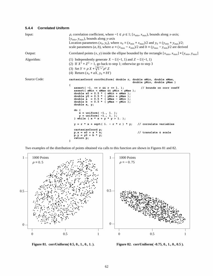
5.4.4 Correlated Unif orm
Input: ρ, correlation coefficient, where−1 ≤ ρ ≤ 1; [xmin, xmax), bounds alongx-axis;[ymin, ymax), bounds alongy-axisLocation parameters (x0, y0), wherex0 = (xmin + xmax)/2 andy0 = (ymin + ymax)/2;scale parameters (a, b), wherea = (xmax − xmin)/2 andb = (ymax − ymin)/2 are derived
Output: Correlated points (x, y) inside the ellipse bounded by the rectangle [xmin, xmax] × [ymin, ymax]
Algorithm: (1) Independently generateX ~ U(−1, 1) andZ ~ U(−1, 1)(2) If X2 + Z2 > 1, go back to step 1; otherwise go to step 3
(3) Set Y = ρ X + √ 1 − ρ2 Z(4) Return (x0 + aX, y0 + bY)
Source Code: cartesianCoord corrUniform( double r, double xMin, double xMax,double yMin, double yMax )
{assert( -1. <= r && r <= 1. ); // bounds on corr coeffassert( xMin < xMax && yMin < yMax );double x0 = 0.5 * ( xMin + xMax );double y0 = 0.5 * ( yMin + yMax );double a = 0.5 * ( xMax - xMin );double b = 0.5 * ( yMax - yMin );double x, y;
do {x = uniform( -1., 1. );y = uniform( -1., 1. );
} while ( x * x + y * y > 1. );
y = r * x + sqrt( 1. - r * r ) * y; // correlate variables
cartesianCoord p;p.x = x0 + a * x; // translate & scalep.y = y0 + b * y;return p;
}
Tw o examples of the distribution of points obtained via calls to this function are shown in Figures 81 and 82.
0 0.5 1
0
0.5
1
•
•
•
•
•
•
•
•
•
•
•
•
•
•
•
•
• ••
•
• •
•
•
•
•
•
•
•
•
•
•
•
•
•
•
•
•
••
•
•
•
•
•
•
•
•
•
•
•
•
•
•
• •
•
••
•
•
•
•
••
•
•
•
••
•
•
•
••
•
•
•
•
•
•
•
•
•
•
•
•
•
• •
•
•
•
•
•
•
•
•
•
•
•
•
•
•
•
• •
••
•
•
•
•
•
•
•
•
•
•
•
•
•
•
•
••
•
•
••
•
•
•
••
••
•
•
•
•
•
•
•
•
••
•
•
•
•
•
••
•
•
•
•
•
•
•
•
•
•
•
•
•
•
•
•
•
•
•
••
•
•
•
•
•
••
•
•
•
•
•
•
•
•
•
•
•
• •
• •
•
•
•
••
•
••
•
••
•
•
•
•
•
•
•
•
••
•
•
•
•
•
•
•
•
•
•
•
•
•
••
•
•
•
•
•
•
•
•
•
•
•
•
•
•
•
•
•
•
•
•
•
•
•
•
•
•
•
•
•
•
•
••
•
••
•
•
•
••
•
•
•
•
•
•
•
•
•
•
•
•
•
••
•
•
•
•
•
•
•
•
•
•
•
•
•
•
••
•
•
•
•
•
••
•
•
•
•
•
•
•
•
•
•
• •
•
••
•
•
•
•
•
•
•••
•
•
•• •
•
•
•
•
•
•
•
•
•
•
••
•
•
•
•
•
•
•
•
•
••
•
•• •
•
•
•
•
•
•
•
•
•
•
•
•
•
••
•
•
•
•
• •
•
•
•
••
•
•
•
•
•
•
•
•
•
•
•
•
•
•
•
•
•
•
•
••
•
•
•
•
•
• •
••
•
•
•
•
•
•
•
•
•
•
•
•
••
•
•
•
•
•
•
•
•
•
••
•
•
•
•
•
•
•
•
•
•
•
•
•
•
•
•
•
•
•
•
•
•
•
••
•
•
•
•
•
•
•
•
•
•
•
•
•
•
•
••
•
•
•
•
•
•
•
•
••
•
•
•
•
•
•
•
•
•
•
•
•
•
••
•
•
•
•
••
•
••
•
•
•
••
•
•
•
••
•
•
• •• •
•
•
••
•
•
••
••
••
•
•
•
•
•
•
•
• •
•
•
•
•
•
•
•
•
•
•
••
•
•
•
•
•
•
•
•
•
•
•
••
•
•
•
•
•
•
•
•
•
•
•
•
•
•
•
•
•
••
•
•
•
••
•
•
•
•
•
•
•
•
•
•
•
•
•
•
•
•
•
•
•
•
•
•
••
••
••
•
•••
•
•
•
•
•
•
••
• ••
•
•
•
•
•
•
•
•
•
•
•
•
••
•
••
•
•
•
•
•
•
•
•
•
•
•
•
•
•
••
•
•
•
•
•
• ••
•
•
•
•
•
•
•
•
•
•
•
•
••
•
•
•
•
•
•
•
•
•
•
•
•
•
•
•
•
•
••
•
•
•
•
•
•
•
•
••
•
••
•
•
••
•
•
••
•
•
•
•
•
•
•
•
•
•
•
•
•
•
•
•
•
•
•
•
• •
•
•
•
•
•
•
•
•
••
•
•
•
•
•
•
•
•
•
•
•
•
•
•
•
•
••
•
•
•
•
•
•
•
•
•
••
•
•
••
•
•
•
•
•
•
•
•
•
•
•
•
•
•
••
•
•
••
•
•
•
•
•
•
•
•
•
••
•
•
•
•
•
•
•
•
••
•
•
••
•
•
•
•
•
•
•
•
•
•
•
•
•
••
•
•
•
•
•
•
•
•
•
•
•
•
•
•
••
•
•
•
•
•
•
•
•
•
•
•
•
•
•
•
•
•
•
•
•
•
•
•
•
•
•
•
•
•
•
•
•
•
•
•
•
•
•
•
•
•
•
•
•
•
•
•
•
•
•
••
• •
•
•••
••
•
•
•
•
•
•
•
•
•
•
•
•
•
••
•
•
•
•
•
•
•
•
•
•
••
•
•
•
•
•
•
••
•
•
•
•
•
•
•
•
•
•
•
•
•
•
•
1000 Pointsρ = 0. 5
Figure81. corrUniform( 0.5, 0., 1., 0., 1. ).
•
•
••
•
•
•
•
•
••
•
•
••
•
•
•
•
• ••
•
••
•
•
•
• ••
•
•
••
•
•
•
• •
•
•
••
•
••
•
•
••••
•
••
•
•
••
•
••
•
•
•
•
•
•
•
•
•
••
•
• •
••
•
•
•
•
••
•
••
•
•
•
•
••
••
•
•
•
• •
••
• •
••
•
•• •
•
•
••
•
•
•
••
••
•
• ••
•
••
•
••
••
•• •
• •
•
•
•
•
• •
•
•
•
•
•
•
•
•
•
••
•
•••
••
•
•
•
•
•
•
•
•
•
••
•
•
•
•
•
••
•
••
•
• ••
•
•
•
••
•
•
•
••
•
•
•
•
••
•
•
•
•
•
•
•
•
•
•
•
•
•
•
•
•
•
•
•
•
•
•
•
•
••
•
•
•
•
•
••
•
•
•
•
• •
• •
• •
•
•
•
•
•
•
••
•
• •
•
•
•
•
•
•
••
•
•
•••
••
•
• •
•
•
••
••
••
••
•
••
•
•
•
•
•
•
• •
••
•
•
•
•
•
•
•
••
•
•
•
•
•
•
•
•
•
•
••
••
•
••
••
•
•
•
•
•
•
•
••
••
•
•
• •
•
•
•
•
•
•
•
•
••
•
•
••
•
•
•
•
••
••
•
•
•
•
•
•
•
•
•
•
••
••
•
•
•
•••
•
•
••
•
•
••
••
••
•
•
•
•
•
•
•
•
•
•
•
•
•
•••
••
•
•
•
•
•
•
••
•
•
•
••
•
•
•
•
••
•
•
•
•
•
• •
•
•
•
•
•
•
•
•
•
•
•
•
•
•
•
•
••
•
•
•
•
••
•
•
•
•
•
•
••
•
•
•
•
•
••
•
•
•
•
•
•
•
•
•
••
••
•
•
•
•
•
••
•
•
••
•
•
••
• •
••
•
•
•
••
• •
•
•
•
••
•
•
•
•
•
•
•
•
•
• •
•
•
•
•
•
•
•
•
•
•
•
••
•
•
••
••
•
••
•••
•
••
•
•
•
•
•
•
•
•
•
••
•
•
•
••
•
•
••
••
••
•
•
•
•
••
•
•
•
•
••
••
•
•
••
•
•
•
••
• •
••
•
•
•
••
•
•
•
•• •
•
•
•
•
•
•
•
•
••
•
•
• •
•
•
•
•
•
•
•
• •
••
• ••
•
••
••
•
•
•
•
•
•
••
••
••
••
•
•
•••
••
•
•
•
•
•
•
••
•
••
• ••
•
•
••
• ••
••
•
••
•
•
•
•
•
•
•
•
•
•
•
•
•
• •
•
•
••
•
•
••
••
•
••
•
••
•
•
•
•
•
•
••
•
•
••
•
•
•
•
•
•
•
•
•
•
•
••
•
• •
•
•
•
•
•
••
•
••
•
••
•
•
••
• ••
•
•
•
•
•
•
•
•
•
•
••
•
•
•
•
••
•
•
•
•
•
•
•
••
•
• •
•••
•••
• •
•
•
••
•
•
•
•
••
••
•
•
•
•
•
••
• •
•
•
•
•
•
•
• •
•
•
•••
• ••
•
•
•
•
•
••
••
•
•
• •
•
•
• •
•
•
•
•
•
•
•
•
• •
••
•
•
•
•
•
•
•
•
•
•
•
•
•••
•
•
••
•
••
••
•
•
•
••
•
•
•
•
•
•
•
•
•
•
•
•
••
•
•
• •
•
•
•
•
•
•
••
•
•
•
•
•
•
•
•
• •
•
•••
•
•
•
•
•
•••
•
•
••
•
•
•
••
•
• •
•
•
•
••
•
•
•
••
••
•
•
•
• •
•
•
•
••
•
•
•
0 0.5 1
0
0.5
1 1000 Pointsρ = − 0. 75
Figure82. corrUniform( -0.75, 0., 1., 0., 0.5 ).
62
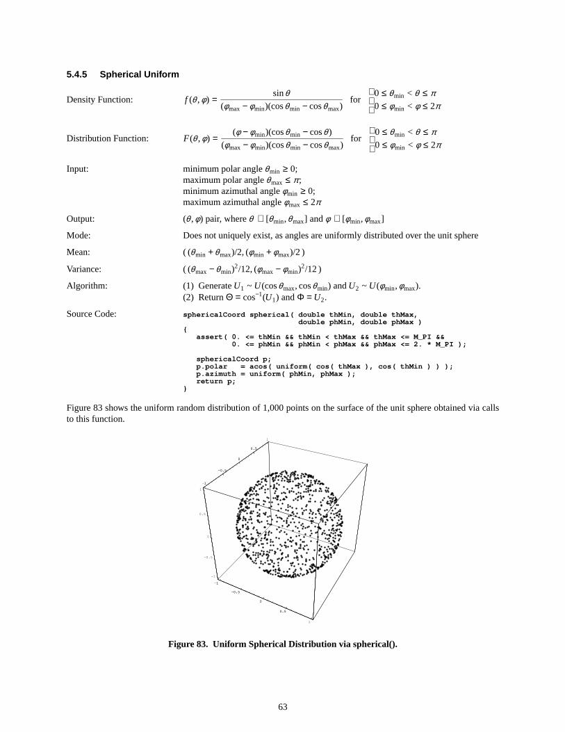
5.4.5 Spherical Unif orm
Density Function: f (θ ,φ) =sinθ
(φmax − φmin)(cosθmin − cosθmax)for
0 ≤ θmin < θ ≤ π0 ≤ φmin < φ ≤ 2π
Distribution Function: F(θ ,φ) =(φ − φmin)(cosθmin − cosθ )
(φmax − φmin)(cosθmin − cosθmax)for
0 ≤ θmin < θ ≤ π0 ≤ φmin < φ ≤ 2π
Input: minimum polar angleθmin ≥ 0;maximum polar angleθmax ≤ π;minimum azimuthal angleφmin ≥ 0;maximum azimuthal angleφmax ≤ 2π
Output: (θ ,φ) pair, whereθ ∈ [θmin,θmax] andφ ∈ [φmin,φmax]
Mode: Does not uniquely exist, as angles are uniformly distributed over the unit sphere
Mean: ( (θmin + θmax)/2, (φmin + φmax)/2 )
Variance: ( (θmax − θmin)2/12, (φmax − φmin)2/12 )
Algorithm: (1) GenerateU1 ~ U(cosθmax, cosθmin) andU2 ~ U(φmin,φmax).(2) Return Θ = cos−1(U1) andΦ = U2.
Source Code: sphericalCoord spherical( double thMin, double thMax,double phMin, double phMax )
{assert( 0. <= thMin && thMin < thMax && thMax <= M_PI &&
0. <= phMin && phMin < phMax && phMax <= 2. * M_PI );
sphericalCoord p;p. pol ar = acos( uniform( cos( thMax ), cos( thMin ) ) );p.azimuth = uniform( phMin, phMax );return p;
}
Figure 83 shows the uniform random distribution of 1,000 points on the surface of the unit sphere obtained via callsto this function.
-1
-0.5
0
0.5
1
-1
-0.5
0
0.5
1
-1
-0.5
0
0.5
1
-1
-0.5
0
0.5
1
-1
-0.5
0
0.5
1
Figure83. Uniform Spherical Distribution via spherical().
63

5.4.6 Spherical Unif orm in N-Dimensions
This will generate uniformly distributed points on the surface of the unit sphere in n dimensions. Whereas the previ-ous distribution (5.4.5) is designed to return the location angles of the points on the surface of the three–dimensionalunit sphere, this distribution returns the Cartesian coordinates of the points and will work for an arbitrary number ofdimensions.
Input: VectorX to receive values; number of dimensionsn
Output: VectorX of unit length (i.e.,X21 + . . . + X2
n = 1)
Algorithm: (1) Generate n IID normal variatesX1, . . . , Xn ~ N(0, 1)
(2) Compute the distance from the origin,d = √ X2i + . . . + X2
n
(3) Return vectorX/d, which now has unit length
Source Code: void sphericalND( double x[], // x array returns pointi nt n ) / / n i s number of dimensions
{// generate a point inside the unit n-sphere by normal polar method
double r2 = 0.;for ( int i = 0; i < n; i++ ) {
x[ i ] = normal();r2 += x[ i ] * x[ i ];
}
// project the point onto the surface of the n-sphere by scaling
const double A = 1. / sqrt( r2 );for ( int i = 0; i < n; i++ ) x[ i ] *= A;
}
Notes: (1) Whenn = 1, this returns {− 1,+1}.(2) When n = 2, it generates coordinates of points on the unit circle.(3) When n = 3, it generates coordinates of points on the unit 3-sphere.
64
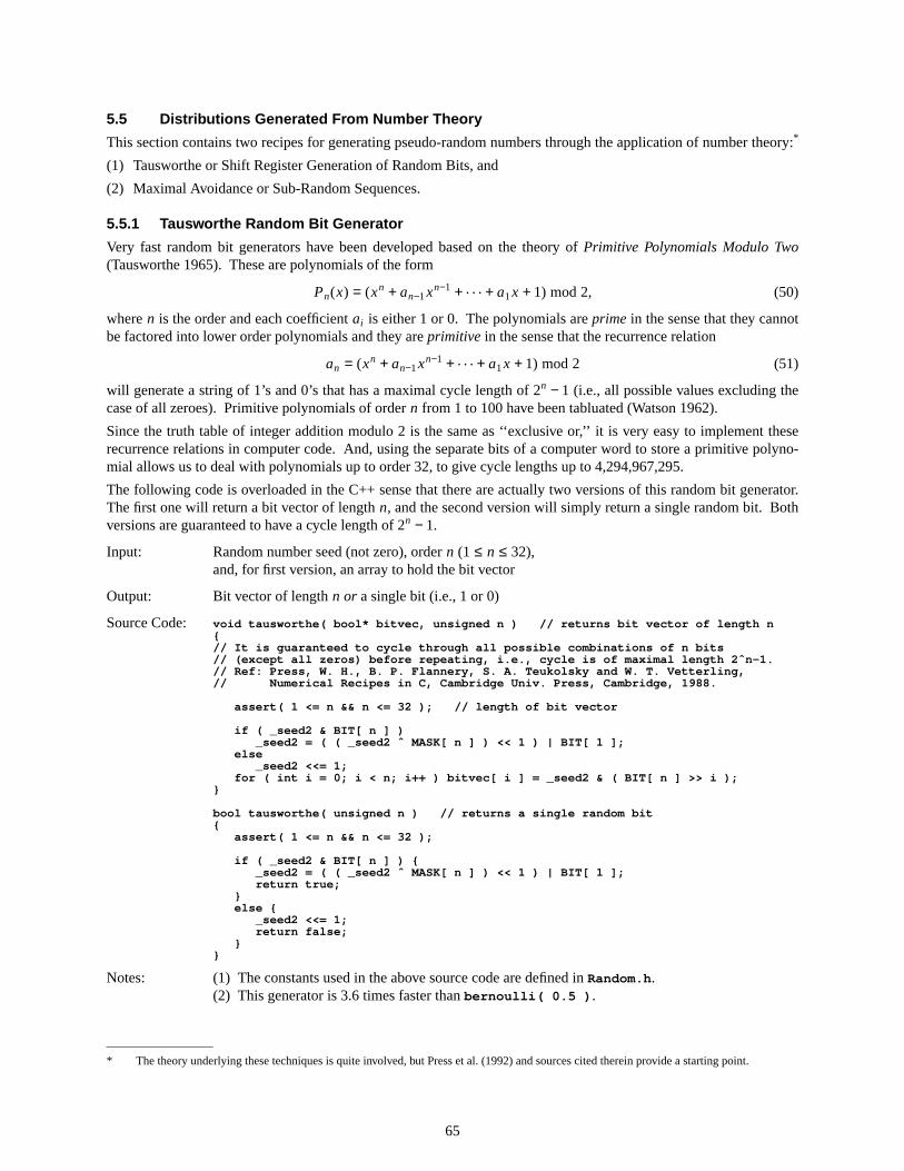
5.5 Distributions Generated Fr om Number Theor y
This section contains two recipes for generating pseudo-random numbers through the application of number theory:*
(1) Tausworthe or Shift Register Generation of Random Bits, and
(2) Maximal Av oidance or Sub-Random Sequences.
5.5.1 Tausworthe Random Bit Generator
Very fast random bit generators have been developed based on the theory of Primitive Polynomials Modulo Two(Tausworthe 1965).These are polynomials of the form
Pn(x) = (xn + an−1xn−1 + . . . + a1x + 1) mod 2, (50)
wheren is the order and each coefficient ai is either 1 or 0. The polynomials are prime in the sense that they cannotbe factored into lower order polynomials and they areprimitive in the sense that the recurrence relation
an = (xn + an−1xn−1 + . . . + a1x + 1) mod 2 (51)
will generate a string of 1’s and 0’s that has a maximal cycle length of 2n − 1 (i.e., all possible values excluding thecase of all zeroes).Primitive polynomials of ordern from 1 to 100 have been tabluated (Watson 1962).
Since the truth table of integer addition modulo 2 is the same as ‘‘exclusive or,’’ it is very easy to implement theserecurrence relations in computer code. And, using the separate bits of a computer word to store a primitive polyno-mial allows us to deal with polynomials up to order 32, to give cycle lengths up to 4,294,967,295.
The following code is overloaded in the C++ sense that there are actually two versions of this random bit generator.The first one will return a bit vector of length n, and the second version will simply return a single random bit. Bothversions are guaranteed to have a cycle length of 2n − 1.
Input: Random number seed (not zero), ordern (1 ≤ n ≤ 32),and, for first version, an array to hold the bit vector
Output: Bit vector of lengthn or asingle bit (i.e., 1 or 0)
Source Code: void tausworthe( bool* bitvec, unsigned n ) // returns bit vector of length n{// It is guaranteed to cycle through all possible combinations of n bits// (except all zeros) before repeating, i.e., cycle is of maximal length 2ˆn-1.// Ref: Press, W. H., B. P. Flannery, S. A. Teukolsky and W. T. Vetterling,/ / Numer i cal Recipes in C, Cambridge Univ. Press, Cambridge, 1988.
assert( 1 <= n && n <= 32 ); // length of bit vector
if ( _seed2 & BIT[ n ] )_seed2 = ( ( _seed2 ˆ MASK[ n ] ) << 1 ) | BIT[ 1 ];
else_seed2 <<= 1;
for ( int i = 0; i < n; i++ ) bitvec[ i ] = _seed2 & ( BIT[ n ] >> i );}
bool tausworthe( unsigned n ) // returns a single random bit{
assert( 1 <= n && n <= 32 );
if ( _seed2 & BIT[ n ] ) {_seed2 = ( ( _seed2 ˆ MASK[ n ] ) << 1 ) | BIT[ 1 ];return true;
}else {
_seed2 <<= 1;return false;
}}
Notes: (1) The constants used in the above source code are defined inRandom.h .(2) This generator is 3.6 times faster thanbernoulli( 0.5 ) .
* The theory underlying these techniques is quite involved, but Press et al. (1992) and sources cited therein provide a starting point.
65
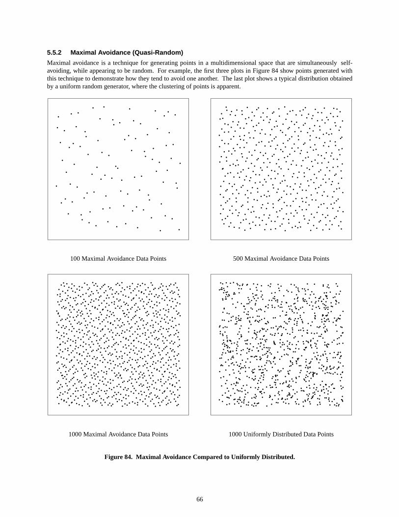
5.5.2 Maximal Av oidance (Quasi-Random)
Maximal avoidance is a technique for generating points in a multidimensional space that are simultaneously self-avoiding, while appearing to be random. For example, the first three plots in Figure 84 show points generated withthis technique to demonstrate how they tend to avoid one another. The last plot shows a typical distribution obtainedby a uniform random generator, where the clustering of points is apparent.
Figure84. Maximal Av oidance Compared to Uniformly Distrib uted.
•
•
•
•
•
•
•
•
•
•
•
•
•
•
•
•
•
•
•
•
•
•
•
•
•
•
•
•
•
•
•
•
•
•
•
•
•
•
•
•
•
•
•
•
•
•
•
•
•
•
•
•
•
•
•
•
•
•
•
•
•
•
•
•
•
•
•
•
•
•
•
•
•
•
•
•
•
•
•
•
•
•
•
•
•
•
•
•
•
•
•
•
•
•
•
•
•
•
•
•
100 Maximal Avoidance Data Points
•
•
•
•
•
•
•
•
•
•
•
•
•
•
•
•
•
•
•
•
•
•
•
•
•
•
•
•
•
•
•
•
•
•
•
•
•
•
•
•
•
•
•
•
•
•
•
•
•
•
•
•
•
•
•
•
•
•
•
•
•
•
•
•
•
•
•
•
•
•
•
•
•
•
•
•
•
•
•
•
•
•
•
•
•
•
•
•
•
•
•
•
•
•
•
•
•
•
•
•
•
•
•
•
•
•
•
•
•
•
•
•
•
•
•
•
•
•
•
•
•
•
•
•
•
•
•
•
•
•
•
•
•
•
•
•
•
•
•
•
•
•
•
•
•
•
•
•
•
•
•
•
•
•
•
•
•
•
•
•
•
•
•
•
•
•
•
•
•
•
•
•
•
•
•
•
•
•
•
•
•
•
•
•
•
•
•
•
•
•
•
•
•
•
•
•
•
•
•
•
•
•
•
•
•
•
•
•
•
•
•
•
•
•
•
•
•
•
•
•
•
•
•
•
•
•
•
•
•
•
•
•
•
•
•
•
•
•
•
•
•
•
•
•
•
•
•
•
•
•
•
•
•
•
•
•
•
•
•
•
•
•
•
•
•
•
•
•
•
•
•
•
•
•
•
•
•
•
•
•
•
•
•
•
•
•
•
•
•
•
•
•
•
•
•
•
•
•
•
•
•
•
•
•
•
•
•
•
•
•
•
•
•
•
•
•
•
•
•
•
•
•
•
•
•
•
•
•
•
•
•
•
•
•
•
•
•
•
•
•
•
•
•
•
•
•
•
•
•
•
•
•
•
•
•
•
•
•
•
•
•
•
•
•
•
•
•
•
•
•
•
•
•
•
•
•
•
•
•
•
•
•
•
•
•
•
•
•
•
•
•
•
•
•
•
•
•
•
•
•
•
•
•
•
•
•
•
•
•
•
•
•
•
•
•
•
•
•
•
•
•
•
•
•
•
•
•
•
•
•
•
•
•
•
•
•
•
•
•
•
•
•
•
•
•
•
•
•
•
•
•
•
•
•
•
•
•
•
•
•
•
•
•
•
•
•
•
•
•
•
•
•
•
•
•
•
•
•
••
•
•
•
•
•
•
•
•
•
•
•
•
•
•
•
•
•
•
•
•
•
•
•
•
•
•
•
•
•
•
•
•
•
•
•
•
•
•
•
•
•
•
•
•
•
•
•
•
•
•
•
•
•
•
•
•
•
•
•
•
•
•
•
•
•
•
•
•
•
•
•
•
•
•
•
•
•
•
•
•
•
•
•
•
•
•
•
•
•
•
•
•
•
•
•
•
•
•
•
•
•
•
•
•
•
•
•
•
•
•
•
•
•
•
•
•
•
•
•
•
•
•
•
•
•
•
•
•
•
•
•
•
•
•
•
•
•
•
•
•
•
•
•
•
•
•
•
•
•
•
•
•
•
•
•
•
•
•
•
•
•
•
•
•
•
•
•
•
•
•
•
•
•
•
•
•
•
•
•
•
•
•
•
•
•
•
•
•
•
•
•
•
•
•
•
•
•
•
•
•
•
•
•
•
•
•
•
•
•
•
•
•
•
•
•
•
•
•
•
•
•
•
•
•
•
•
•
•
•
•
•
•
•
•
•
•
•
•
•
•
•
•
•
•
•
•
•
•
•
•
•
•
•
•
•
•
•
•
•
•
•
•
•
•
•
•
•
•
•
•
•
•
•
•
•
•
•
•
•
•
•
•
•
•
•
•
•
•
•
•
•
•
•
•
•
•
•
•
•
•
•
•
•
•
•
•
•
•
•
•
•
•
•
•
•
•
•
•
•
•
•
•
•
•
•
•
•
•
•
•
•
•
•
•
•
•
•
•
•
•
•
•
•
•
•
•
•
•
•
•
•
•
•
•
•
•
•
•
•
•
•
•
•
•
•
•
•
•
•
•
•
•
•
•
•
•
•
•
•
•
•
•
•
•
•
•
•
•
•
•
•
•
•
•
•
•
•
•
•
•
•
•
•
•
•
•
•
•
•
•
•
•
•
•
•
•
•
•
•
•
•
•
•
•
•
•
•
•
•
•
•
•
•
•
•
•
•
•
•
•
•
•
•
•
•
•
•
•
•
•
•
•
•
•
•
•
•
•
•
•
•
•
•
•
•
•
•
•
•
•
•
•
•
•
•
•
•
•
•
•
•
•
•
•
•
•
•
•
•
•
•
•
•
•
•
•
•
•
•
•
•
•
•
•
•
•
•
•
•
•
•
•
•
•
•
•
•
•
•
•
1000 Maximal Avoidance Data Points
•
•
•
•
•
•
•
•
•
•
•
•
•
•
•
•
•
•
•
•
•
•
•
•
•
•
•
•
•
•
•
•
•
•
•
•
•
•
•
•
•
•
•
•
•
•
•
•
•
•
•
•
•
•
•
•
•
•
•
•
•
•
•
•
•
•
•
•
•
•
•
•
•
•
•
•
•
•
•
•
•
•
•
•
•
•
•
•
•
•
•
•
•
•
•
•
•
•
•
•
•
•
•
•
•
•
•
•
•
•
•
•
•
•
•
•
•
•
•
•
•
•
•
•
•
•
•
•
•
•
•
•
•
•
•
•
•
•
•
•
•
•
•
•
•
•
•
•
•
•
•
•
•
•
•
•
•
•
•
•
•
•
•
•
•
•
•
•
•
•
•
•
•
•
•
•
•
•
•
•
•
•
•
•
•
•
•
•
•
•
•
•
•
•
•
•
•
•
•
•
•
•
•
•
•
•
•
•
•
•
•
•
•
•
•
•
•
•
•
•
•
•
•
•
•
•
•
•
•
•
•
•
•
•
•
•
•
•
•
•
•
•
•
•
•
•
•
•
•
•
•
•
•
•
•
•
•
•
•
•
•
•
•
•
•
•
•
•
•
•
•
•
•
•
•
•
•
•
•
•
•
•
•
•
•
•
•
•
•
•
•
•
•
•
•
•
•
•
•
•
•
•
•
•
•
•
•
•
•
•
•
•
•
•
•
•
•
•
•
•
•
•
•
•
•
•
•
•
•
•
•
•
•
•
•
•
•
•
•
•
•
•
•
•
•
•
•
•
•
•
•
•
•
•
•
•
•
•
•
•
•
•
•
•
•
•
•
•
•
•
•
•
•
•
•
•
•
•
•
•
•
•
•
•
•
•
•
•
•
•
•
•
•
•
•
•
•
•
•
•
•
•
•
•
•
•
•
•
•
•
•
•
•
•
•
•
•
•
•
•
•
•
•
•
•
•
•
•
•
•
•
•
•
•
•
•
•
•
•
•
•
•
•
•
•
•
•
•
•
•
•
•
•
•
•
•
•
•
•
•
•
•
•
•
•
•
•
•
•
•
•
•
•
•
•
•
•
•
••
•
•
•
•
•
•
•
•
•
•
•
•
•
•
•
•
•
•
•
•
500 Maximal Avoidance Data Points
•
••
••
•
•
•
•
•
•
•
•
•
•
•
•
••
•
••
•
•
•
•
•
•
•
••
•
•
•
• •
•
•
•
•
••
••
•
•
•
•
• •
•
•
•
•
•
•
• ••
•
•
•
••••
•
•
•
•
•
•
•
•
•
•
•
••
••
•
•
•
•
•
•
• •
•
•
••
•
••
•
••
•
•
•
•
•
•
••
••
•
•
•
•
•
•
•
•
•
•
•
•
•
••
•
•
•
•
••
•
•
•
•
•
••
•
•
•
•
•
•
•
•
••
•
•
•
•
•
•
•
•
•
•
••
•
•
•
•
•
•
•
•
•
•
•
•
•
•
•
•
•
•
••
•
•
•
•
•
•
•
• •
•
•
•
•
• •
•
•
•
•
•
•
• •
•
•
••
•
•
•
•
•
•
•
• • •
•
•
••
••
•
•
•
•••
•
•
•
•
•
•
•
••
••
••
•
•
•
•
•
•
•
•
•
•
•
•
•
•
•
•
•
•
••
•
•
•
•
••
•• •
•
•
•
•
•
•
•
••
•
•
•
•
•
•
•
•
• •
•
•
•
•
•
•
•
•
•
•
•
•••
• •
•
•
•
•
•
•
•
••
•
•
•
•
•
•
•
•
• •
•
•
•
• •
••
•
•
•
•
•
•
•
•
•
•
•
•
•
•
• •
•
••
•
•
•
•
••
•
•
•
• •
•
•
•
•
•
•
•
•
•
•
•
••
•
•
•
•
•
•
•
•
•
•
•
•
•
•
•
•
•
•
•
••
•
•
•
•
•
•
•
•
••
•
•
•••
•
•
•
•
•
•
•
•
•
•
•
•
•
•
•
•
•
•
•
••
•
•• •
•
•
•
•
•
•
•
•
••
•
•
•
•
•
••
•
••
•
•
•
•
•
•
•
•
••
•
•
•
•
•
•
•
•
•
•
•
•
•
•
•
•
••
•
•
•
•
•
•
•
•
•
•
•
•
•
•
•
•
•
•
••
•
•
•
•
•
•
•
•
•
•
•
•
•
•
•
•
•
•
•
•
•
•
•
•
•
••
••
•
•
•
•
•
•
•
•
•
•
•
•
• •
•
•
••
•
•
•
•
•
•
•
•
•
••
•
•
•
•
•
•
•
•
•
•
•
•
•
• •
•
•
•
•
•
•
••
•
•
•
•
•
••
•
•
•
••
•
•
•
•
•
•
•
•
••
•
•
•
•
•
• •
•
•
•
• •
•
•
•
•
•
•
•
•
•
•
•
•
•
•
•
•
••
•
•
•
••
•
•
•
•
•
•
•
••
•
•
•
•
•
•
••
•
•
••
••
•
•
•
•
•
•
•
•
•
•
•
•
•
•
•
•
•
•
•
•
•
•
•
•
•
•
•
•
•
•
•
•
•
•
•
•
••
•
•
•
•
•
•
•
••
••
••
•
•
•
•
•
•
•
•
•
•
•
•
•
•
•
•
•
•
•
•
•
•
•
•
•
•
•
•
••
•
•
•
••
•
• •
•
•
•
•
•
•
•
•
•
•
•
•
•
•
•
•
•
•
•
•
••
•
•
•
•
•
•
•
• ••
•
•
•
••
•
•
•
•
•
•
•
•
•
•
•
•
•
•
•
••
•
•
•
•
•
•
•
••
•
•
•
• ••
••
•
•
•
•
•
•
•
•
•
•
•
•
•
•
•
•
••
•
••
•
•
•
•
•
•
•
•
•
•
•
••
••
•
•
••
•
•
•
•
•
•
•
• •
••
•
•• •
•
•
•
•
•
•
•
•
•
•
•
•
•
•
•
•
•
• •
•
•
•
•
•
•
•
• •
•
••
•
•
•
•
•
••
•
•
•
•
••
•
•
•
•
•
•
•
•
•
•
•
•
•
•
•
•
•
•
•
•
•
•
•
•
•
•
•
•
•
•
•
•
•
•
•
•
•
•
•
••
•
•
•
•
•
•
•
• •
••
•
•
•
•
•
•
•
•
•
•
•
••
•
•
•
•
•
•
•
•
•
•
••
1000 Uniformly Distributed Data Points
66
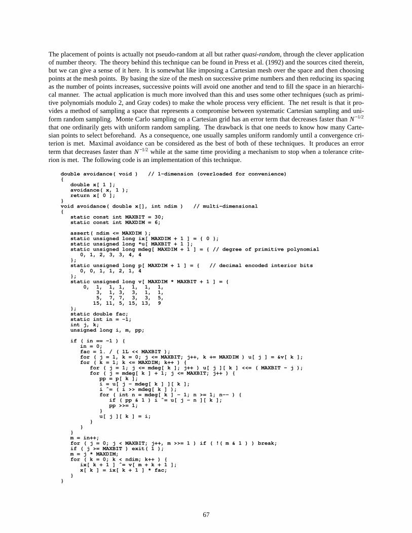
The placement of points is actually not pseudo-random at all but rather quasi-random, through the clever applicationof number theory. The theory behind this technique can be found in Press et al. (1992) and the sources cited therein,but we can give a sense of it here. It is somewhat like imposing a Cartesian mesh over the space and then choosingpoints at the mesh points. By basing the size of the mesh on successive prime numbers and then reducing its spacingas the number of points increases, successive points will avoid one another and tend to fill the space in an hierarchi-cal manner. The actual application is much more involved than this and uses some other techniques (such as primi-tive polynomials modulo 2, and Gray codes) to make the whole process very efficient. The net result is that it pro-vides a method of sampling a space that represents a compromise between systematic Cartesian sampling and uni-form random sampling. Monte Carlo sampling on a Cartesian grid has an error term that decreases faster than N−1/2
that one ordinarily gets with uniform random sampling. The drawback is that one needs to know how many Carte-sian points to select beforehand. As a consequence, one usually samples uniform randomly until a convergence cri-terion is met. Maximal avoidance can be considered as the best of both of these techniques. It produces an errorterm that decreases faster than N−1/2 while at the same time providing a mechanism to stop when a tolerance crite-rion is met.The following code is an implementation of this technique.
double avoidance( void ) // 1-dimension (overloaded for convenience){
double x[ 1 ];avoidance( x, 1 );return x[ 0 ];
}void avoidance( double x[], int ndim ) // multi-dimensional{
static const int MAXBIT = 30;static const int MAXDIM = 6;
assert( ndim <= MAXDIM );static unsigned long ix[ MAXDIM + 1 ] = { 0 };static unsigned long *u[ MAXBIT + 1 ];static unsigned long mdeg[ MAXDIM + 1 ] = { // degree of primitive polynomial
0, 1, 2, 3, 3, 4, 4};static unsigned long p[ MAXDIM + 1 ] = { // decimal encoded interior bits
0, 0, 1, 1, 2, 1, 4};static unsigned long v[ MAXDIM * MAXBIT + 1 ] = {
0, 1, 1, 1, 1, 1, 1,3, 1, 3, 3, 1, 1,5, 7, 7, 3, 3, 5,
15, 11, 5, 15, 13, 9};static double fac;static int in = -1;int j, k;unsigned long i, m, pp;
if ( in == -1 ) {in = 0;fac = 1. / ( 1L << MAXBIT );for ( j = 1, k = 0; j <= MAXBIT; j++, k += MAXDIM ) u[ j ] = &v[ k ];for ( k = 1; k <= MAXDIM; k++ ) {
for ( j = 1; j <= mdeg[ k ]; j++ ) u[ j ][ k ] <<= ( MAXBIT - j );for ( j = mdeg[ k ] + 1; j <= MAXBIT; j++ ) {
pp = p[ k ];i = u[ j - mdeg[ k ] ][ k ];i ˆ = ( i >> mdeg[ k ] );for ( int n = mdeg[ k ] - 1; n >= 1; n-- ) {
if ( pp & 1 ) i ˆ= u[ j - n ][ k ];pp >>= 1;
}u[ j ][ k ] = i;
}}
}m = i n++;for ( j = 0; j < MAXBIT; j++, m >>= 1 ) if ( !( m & 1 ) ) break;if ( j >= MAXBIT ) exit( 1 );m = j * MAXDIM;for ( k = 0; k < ndim; k++ ) {
ix[ k + 1 ] ˆ= v[ m + k + 1 ];x[ k ] = ix[ k + 1 ] * fac;
}}
67

6. DISCUSSION AND EXAMPLES
This section presents some example applications in order to illustrate and facilitate the use of the various distribu-tions. Certain distributions, such as the normal and the Poisson, are probably over used and others, due to lack offamiliarity, are probably under used. In the interests of improving this situation, the examples make use of the lessfamiliar distributions. Before we present example applications, however, we first discuss some differences betweenthe discrete distributions.
6.1 Making Sense of the Discrete Distrib utions
Due to the number of different discrete distributions, it can be a little confusing to know when each distribution isapplicable. To help mitigate this confusion, let us illustrate the difference between the binomial, geometric, negativebinomial, and Pascal distributions. Consider, then, the following sequence of trials, where ‘‘1’ ’ signifies a successand ‘‘0’ ’ a failure.
Tr ial: 1 2 3 4 5 6 7 8Outcome: 1 0 1 1 1 0 0 1
The binomial(n, p) represents the number of successes inn trials so it would evaluate as follows.
binomial( 1 , p ) = 1binomial( 2 , p ) = 1binomial( 3 , p ) = 2binomial( 4 , p ) = 3binomial( 5 , p ) = 4binomial( 6 , p ) = 4binomial( 7 , p ) = 4binomial( 8 , p ) = 5
The geometric (p) represents the number of failures before the first success. Since we have a success on the firsttrial, it evaluates as follows.
geometric( p ) = 0
The negativeBinomial (s, p) represents the number of failures before the sth success in n trials so it would evaluateas follows.
negativeBinomial( 1 , p ) = 0negativeBinomial( 2 , p ) = 1negativeBinomial( 3 , p ) = 1negativeBinomial( 4 , p ) = 1negativeBinomial( 5 , p ) = 3
The pascal(s, p) represents the number of trials in order to achieve s successes so it would evaluate as follows.
pascal( 1 , p ) = 1pascal( 2 , p ) = 3pascal( 3 , p ) = 4pascal( 4 , p ) = 5pascal( 5 , p ) = 8
68

6.2 Adding Ne w Distrib utions
We show here how it is possible to extend the list of distributions. Suppose that we want to generate random num-bers according to the probability density function shown in Figure 85.
-1 -0.5 0 0.5 1
0
0.25
0.5
f (x)
x
Figure85. Semi-Elliptical Density Function.
The figure is that of a semi-ellipse, and its equation is
f (x) =2
π√ 1 − x2, where − 1 ≤ x ≤ 1. (52)
Integrating, we find that the cumulative distribution function is
F(x) =1
2+
x√ 1 − x2 + sin−1(x)
π, where − 1 ≤ x ≤ 1. (53)
Now, this expression involves trancendental functions in a nonalgebraic way, which precludes inverting. But, we canstill use the acceptance-rejection method to turn this into a random number generator. Wehav e to do two things.
(1) Definea function that returns a value fory, giv en avalue forx.
(2) Defineacircular distribution that passes the function pointer to theUser-Specifieddistribution.
Here is the resulting source code in a form suitable for inclusion in the Random class.
double ellipse( double x, double, double ) // Ellipse Function{
return sqrt( 1. - x * x ) / M_PI_2;}
double Random::elliptical( void ) // Elliptical Distribution{
const double X_MIN = -1.;const double X_MAX = 1.;const double Y_MIN = 0.;const double Y_MAX = 1. / M_PI_2;
return userSpecified( ellipse, X_MIN, X_MAX, Y_MIN, Y_MAX );}
And here is source code to makeuse of this distribution.
#include <iostream.h>#include "Random.h"
void main( void ){
Random rv;for ( int i = 0; i < 1000; i++ ) cout << rv.elliptical() << endl;
}
69

6.3 Bootstrap Method as an Application of Sampling
If we are only interested in the mean value,x, of a set of data and wish to know the accuracy of the sample mean,then there is a handy formula available:
Standard Error of the Mean=
1
N(N − 1)
N
i =1Σ (xi − x)2
1/2
. (54)
On the other hand, if we are interested in some other metric, such as the correlation coefficient, then there is no sim-ple analytical formula that allows us to estimate the error. The bootstrap method was designed to address this situa-tion. The basic idea is that we sample the original data with replacement to obtain a synthetic data set of another Ndata points, and, from this, we compute the statistic we are interested in. We then repeat this process over and overuntil we have built up a set M of computed values of the relevant statistic. We then compute the standard deviationof these M values; it will provide the standard error of the statistic. Given the high cost and consequent scarcity ofdata in many applications, combined with the reduced cost and abundance of computing power, the bootstrapmethod becomes a very attractive technique for extracting information from empirical data (Diaconis and Efron1983; Efron and Tibshirani 1991).TheNew York Timeshad this to say:
A new technique that involves powerful computer calculations is greatly enhancing the statisticalanalysis of problems in virtually all fields of science. The method, which is now surging intopractical use after a decade of refinement, allows statisticians to determine more accurately thereliability of data analysis in subjects ranging from politics to medicine to particle physics....(Nov. 8, 1988, C1, C6).
Here, we give an example of how sampling may be applied to empirical data in order to compute a bootstrap errorestimate. The data consist of 150 spall fragments that were collected when a penetrator perforated a plate of armor.Each spall fragment was weighed and the dimensionless shape factor (see section 3.7 for the definition) was mea-sured from 16 different directions in order to compute an average shape factor. Thus, the experimental data consistof 150 mass, average shape factor pairs. The question arises as to whether there is any correlation between mass andav erage shape factor. For example, one might expect small fragments to be more compact and large fragments to bemore irregular in shape. This would be reflected in a positive correlation coefficient. The correlation coefficientcomputed from the original experimental data is −0. 132874. Since the absolute value is considerably smaller than1, there appears to be no correlation between mass of the fragment and its average shape factor.* Now, we would liketo know how much variation to expect in the correlation coefficient. The 150 data pairs were put into a file called‘‘sampleData.’’ The following source code then implements the bootstrap method.
#include <iostream.h>#include "Random.h"
void main( void ){
const int N_DATA = 150; // number of data pointsconst int N_DIMS = 2; // number of dimensionsRandom rv;
double data[ N_DIMS ];for ( int i = 0; i < N_DATA; i++ ) {
rv.sample( data, N_DIMS );cout << data[ 0 ] << " " << data[ 1 ] << endl;
}}
This will generate a synthetic set of 150 data pairs, from which we compute the corresponding correlation coeffi-cient. We then replicate the process 128, 256, 512, and 1,024 times. After 128 replications, we find the followingstatistics on thestate of correlationamong the two variables, shape factor and mass.
* More formally, the value of the t statistic is −1. 63094, and since |− 1. 63094 | < 1. 96, the critical value for a two-sided test at a 0.05 signifi-cance level, it fails the Student t test.Consequently, wecannot reject the null hypothesis that the data pairs are uncorrelated.
70
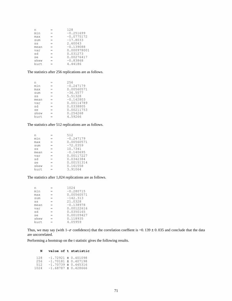
n = 128mi n = -0.251699max = -0.0775172sum = -17.8033ss = 2.60043mean = -0.139088var = 0.000978001sd = 0.031273se = 0.00276417skew = -0.83868kur t = 4.44186
The statistics after 256 replications are as follows.
n = 256mi n = -0.247179max = 0.00560571sum = -36.5577ss = 5.51328mean = -0.142803var = 0.00114789sd = 0.0338805se = 0.00211753skew = 0.254268kur t = 4.59266
The statistics after 512 replications are as follows.
n = 512mi n = -0.247179max = 0.00560571sum = -72.0359ss = 10.7341mean = -0.140695var = 0.00117227sd = 0.0342384se = 0.00151314skew = 0.161558kur t = 3.91064
The statistics after 1,024 replications are as follows.
n = 1024mi n = -0.280715max = 0.00560571sum = -142.313ss = 21.0328mean = -0.138978var = 0.00122616sd = 0.0350165se = 0.00109427skew = 0.118935kur t = 4.05959
Thus, we may say (with 1–σ confidence) that the correlation coeffient is −0. 139 ± 0. 035 and conclude that the dataare uncorrelated.
Performing a bootstrap on the t statistic gives the following results.
N value of t statistic
128 - 1. 72921 ± 0.401098256 - 1. 70181 ± 0.407198512 - 1. 70739 ± 0.445316
1024 - 1. 68787 ± 0.428666
71

6.4 Monte Carlo Sampling to Ev aluate an Integral
A simple application of random number distributions is in the evaluation of integrals. Integration of a function of asingle variable, f (x), is equivalent to evaluating the area that lies below the function. Thus, a simple way to esti-mate the integral
b
a∫ f (x) dx (55)
is to first find the bounding rectangle [a, b] × [0, ymax], as shown in Figure 86; select uniform random points (X,Y)within the rectangle; and, for every point that satisfies the condition Y < f (X), increment the area estimate by theamount (b − a)ymax/N, whereN is the total number of sample points in the bounding rectangle.
a b
ymax
f (x)
x
y
Figure86. Integration as an Area Evaluation via Acceptance-Rejection Algorithm
This can be accomplished with the following source code.
#include <iostream.h>#include "Random.h"
double f( double x ) { return . . . }
void main( void ){
Random rv;
const double A = . . .const double B = . . .const double Y_MAX = . . .const int N = . . .
double area = 0.;for ( int i = 0; i < N; i++ ) {
double x = rv.uniform( A, B );double y = rv.uniform( 0., Y_MAX );if ( y < f( x ) ) area += ( B - A ) * Y_MAX / N;
}cout << "area estimate = " << area << endl;
}
This is essentially a binomial process with a probability of success p equal to the ratio of the area under the curve tothe area of the bounding rectangle.The standard deviation of the area estimate, therefore (see section 5.2.2), is
σ = √ Np(1 − p)
N× area of bounding rectangle. (56)
Note that the factor√ p(1 − p) is close to 0.5 unless we happen to have a very close-fitting bounding rectangle. Thisso-called ‘‘hit-or-miss’’ method is also inefficient in that two calls are made to the random number generator foreach sample point. A more efficient method is obtained by first approximating the integral in eq. (55) by its Rie-mann sum:
72
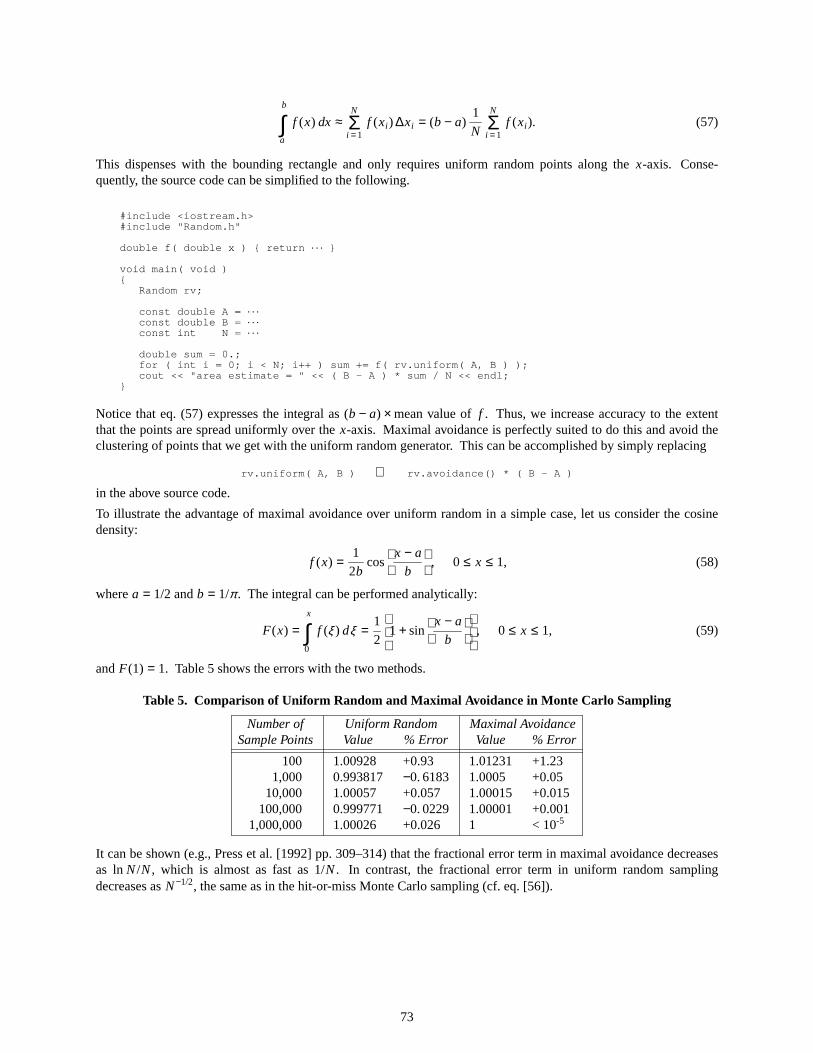
b
a∫ f (x) dx ≈
N
i =1Σ f (xi ) ∆xi = (b − a)
1
N
N
i =1Σ f (xi ). (57)
This dispenses with the bounding rectangle and only requires uniform random points along the x-axis. Conse-quently, the source code can be simplified to the following.
#include <iostream.h>#include "Random.h"
double f( double x ) { return . . . }
void main( void ){
Random rv;
const double A = . . .const double B = . . .const int N = . . .
double sum = 0.;for ( int i = 0; i < N; i++ ) sum += f( rv.uniform( A, B ) );cout << "area estimate = " << ( B - A ) * sum / N << endl;
}
Notice that eq. (57) expresses the integral as (b − a) × mean value of f . Thus, we increase accuracy to the extentthat the points are spread uniformly over the x-axis. Maximal avoidance is perfectly suited to do this and avoid theclustering of points that we get with the uniform random generator. This can be accomplished by simply replacing
rv.uniform( A, B ) ⇒ rv.avoidance() * ( B - A )
in the above source code.
To illustrate the advantage of maximal avoidance over uniform random in a simple case, let us consider the cosinedensity:
f (x) =1
2bcos
x − a
b
, 0 ≤ x ≤ 1, (58)
wherea = 1/2 andb = 1/π. The integral can be performed analytically:
F(x) =x
0∫ f (ξ ) dξ =
1
2
1 + sin
x − a
b, 0 ≤ x ≤ 1, (59)
andF(1) = 1. Table 5 shows the errors with the two methods.
Table 5. Comparison of Uniform Random and Maximal Avoidance in Monte Carlo Sampling
Number of Uniform Random Maximal AvoidanceSample Points Value % Error Value % Error
100 1.00928 +0.93 1.01231 +1.231,000 0.993817 −0. 6183 1.0005 +0.05
10,000 1.00057 +0.057 1.00015 +0.015100,000 0.999771 −0. 0229 1.00001 +0.001
1,000,000 1.00026 +0.026 1 < 10-5
It can be shown (e.g., Press et al. [1992] pp. 309–314) that the fractional error term in maximal avoidance decreasesas ln N/N, which is almost as fast as 1/N. In contrast, the fractional error term in uniform random samplingdecreases asN−1/2, the same as in the hit-or-miss Monte Carlo sampling (cf. eq. [56]).
73

6.5 Application of Stoc hastic Interpolation
The technique of stochastic interpolation is very useful in those cases where the data does not seem to fit any knowndistribution. It allows us to simulate the essential characteristics of the data without returning the same data pointsover and over again. For example, Figure 87 shows bifurcated data in the x–y plane. Without an understanding ofthe underlying mechanism, it would be very difficult to fit a distribution to this data. However, it is easy to createsynthetic realizations using stochastic interpolation. We must first place the data in a file named ‘‘stochasticData.’’Then the following code will produce another realization such as that shown in Figure 88.
#include <iostream.h>#include <stdlib.h>#include <unistd.h>#include "Random.h"
void main( int argc, char* argv[] ){
long seed = long( getpid() );if ( argc == 2 ) seed = atoi( argv[ 1 ] );
Random rv( seed );
for ( int i = 0; i < N_DATA; i++ ) {point p = rv.stochasticInterpolation();cout << p.x << " " << p.y << endl;
}}
••
•
•
•
•
•
•• ••
•
•
•
•
••
•
•
•
•
•
•
•
••
••
•
•
•
•
•
••
•
•
•
•
•
••
•
•
•
•
•
•
•
••
•
•
•
•
•
•
••
•
•
•
•
•
•
•
•
•
•
•
•
•
••
•
•
•
•
••
•
•
•
•
•
•
•
•
•
•
•
•
•
•
•
•
•
•
•
•
•
•
•
•
•
•
•
•
•
•
• •••
•
•
•
••
•
••
•
•
•
•
•
•
•
••
•
•
•
•
•
•
•
•
•
•
•
••
•
• •
•
• •
••
•
•
•
•
•
•
•
•
•
•
•
••
•
••
•
••
••
•
•
•
••
•
•
• •
•
•
••
•
••
•
••
•
••
•
•
•
•
•
••
•
••
•
•
•
• •
•
•
•
•
•
•
•
•
•
•
•
•
••
••
•
•
••
•
••
• •
••
•
•
•• •
•
••
•
••
• •
•
•
••
••
•
•
•
•
••
•
•
•
•
••
•
•
• •
••
•
• •
•
•
•
•
•
•••
•
•
•••
•
•
•
•
••
•
•
••
•
•
•
•
•
•
•
•
•
•
•
•
•
•
•
• •
•
•
••
•
••
•
•
•
•
•
• ••
•
•
•
•
•
•
••
•
•••
•
•
•
•
•
•
•
•
•
•
•
•
•
•
•
••
••
•
•
•
••
•
•
••
•
•
•
•
•
••
••
•• •
•
•
•
•
•
•
•
•
••
•
•
••
•
•
•
••
•
•
•
••
••
•
•
•
•
••
•
•
•
•
•
••••
•
•
•
•
•
•
•
•
•
•••
•
•
•
• •
•
•
•
••
•
••
•
•
•
•
•
••
•
•
••
••
•
•
••
•
••
•
•
•
•
••
•
•
•
••
•
•
•
•
•••
•
•
•
••
•
•
•
•
•
•
••
•
•
•
• •
•
•
••
•
•
•
•
•
••
•
••
••
•
•
•
•
•
•
•
••
••
••
•
••
•
•
•
••
•
•
•• ••
•
•
•
•
•
•
•
•
•
••
•
• •
•
•
•
•
••
•
•
••
••
•
••
••
•
•
•
••
•
••
••
•
•
•
•
•
•
•
•
•
•
••
•
•
•
•
•
•
••
•
•
•
•
•
•
•
•
• •
•
• •
•
••
•
••
•
•
•
••
•
•
•
••
•
•
•
•
•
•
•
•
•
• •
•
••
•
••• ••
•
•
•
•
•
•
•
•
••
•
•
•
•
•
•
•
•
•
••
•
•••
•
•
•
••
•
•
•
•
•
•
•
•
•
•
•
•
•
••••
•
••
•• ••
•
••
•
•
•
•
•
•
•
•
•
•
••
••
•
•
•
•
•
•
•
•
• •
•
•
•
•
•
•
•
•
•
•
•
•
•
••
•
•
•
•
•
•
•
•
•
•
•
•
••
••
•
•
•
•
••
••
••
•
•
•
•
••
•
•
•
•
•
•
•
•
•
••
•
•
•
•
•
•
•
•
•
•
•
•
•
•
•• •
•
•
•
•
•
•
•
•
•
•
•
•
•
•
••
•
•
•
•
•
•
•
•
•
••
•
•
••
•
•
•
•
•
•
•
•
•
•
•
•
•
•
•
•
•
•
•
•
•
•
•
•
•
•
•
•
•
•
•
•
•
•
•
••
•
•
•
•
•
•
••
•
•
•
•
•
••
•
•
•
•
•
•
•
•
•
•
•
•
•
•
••
•
•
•
•• •
•
•
•
•
•
•
•
••
•
•
•
•
•
•
•
••
•
•
•
•
•
•
•
•
•
•
••
•
•
•
••
••
••
•
••
••
•
•
••
•
•
•
•
•
•
•
•
•
•
•
•
•
•
•
•
••
•
•
•
•
• •
•
••
•
•
•
••
-6 -3 0 3 6
-6
-3
0
3
6
Figure87. Stochastic Data for Stochastic Interpolation.
••
•
•
•
•
•
•
•
•
•
•
••
•
•
•
•
•
• •
•
•
•
•
•
•
•
••
•
•••
•
•
•
•
•
•
•
•
•
•
•
•
•
•
••
• •
•
•
•
•
•
•
•
•
•
•
•
••
••
•
•
•
•
•
•
••
••
•
•
•
•
•
•
•
•
•
••
•
•
•
•
•
•
•
•
•
•
•
• •
•
• •
•
•
•
••
•
•
• •
•
•
•
•
•••
•
•
•
•
••
•
• •
•
•
•
•
•
•
• ••
•
•
•
•
•
• •
•
•
•
••
•
•
•
•
•
•
•
•
•
•
•
•
•• •
•
•
•
•••
•
•
••
•
•
•
• •
•
•
•
••
•
•
•
•
•
••
•
•
•
•
•
•
•
•
•
•
• •
•
•
•
•
•
•
•
••
•
•
•
•
•
•
•
•
•
•••
•
••
•
•
•
•
•
••
•
•
••
•
•
•
•
•
•
• •
•
•
•
•
•
•
••
•
•
•
•
• •
•
•
•
•
••
•
••
•
•
•
••
•
•
•
•
•
•
•
•
•
•
•
•
••
•
•
• •
•
•
•
•
•
•
•
•
•
••
•
•
•
•
••
•
•
••
•
•
•
•
•
•
•
•
•
•
•
•
•
•
•
•
•
•
••
•
•
•
•
•
•
•
•
•
•
•
•
•
•
••
••
•
•
••
•
•
•
••
•
•
• •
••
•
•
•
•
•
•
•
•
••
•
•
•
•
•
•
•
•
•
••
•
•
•
••
•
•
•
•
•
•
••
•
•
•
•
•
•
•
••
•
••
•
•
•
•
•
••
•
•
•
•
••
•
•
•
•
•
•
•
•••
•
•
•
•
•
•
•
•
•
•
•
•
•
•
•
•
••
•
••
•
•
•
•
•
••
•
•
•
•
••
••
•
•
•
•
•
••
•
•
•
•
••
•
•
•
•
•
•
• •
•
••
•
•
•
•
•
•
•
•
• • •
•
•
••
•
••
•••
••
•
•
•
•
•
•
•
•
••
•
•
•
•• •
•
•
•
•
•
•• •
••
• ••
•
•
•
•
•
•
•
•
•
•
•
•
•
•
•
•
•
•
•
•
•
•
•
•
•
•
•
•
•
•
•
•
•
•
•
••
••••
•
•
•
• ••
•
•
•••
•••
•
•
••
•
•
•
•
•
•
•
•
•
•
•
•
•
•
• •
•
•
•
•
••
•
•
•
••
•
•
•
•
•
•
•
•
•
••
•
•
•
••
•
• •
•
••
•
• •
•
•
•
•
•
•
••
•
•
••
•
•
• •
•
••
•
•
•• •
••
•
•••
•
•
•
•
•
•
•
•
•
•
•
•
••
•
•
•
•• •
•
•
••• ••
•
•
•
•
•
• •
•
•
••
•
•
•• •
••
•
•
•
•
•
•
••
•
••
• •
••
•
•
••
•
•
•
•
•
•
•
•
•
••
•
••
•
•
•
••
•••
••
•
••
•
•
•
••
•
•
•
•
•
•
•
•
•
•
•
•
•
•
•
•
•
•
•
•
• •
•
••
•
•
•
•
•
••
•
• ••
•
•
•
•
•
•
•
•
•
•
•• •
•
•
•
•
•
•
••
•
•
••
•
•
•
•
•
•
•••
•
•
•
•
•
•
•
•
•
•
•
•
•
• •
••
•
•
•
•
•
•
•
•
•
•
•
•
•
•
•
•••
•
•
•
•
•
• •
•
•
•
•
•
• •
•
•
•
•
•
• •
•
•
•
•
••
•
•
• ••
•
•
•
•
•
•
••
•
•••
•
•
•
••
••
••
•
•
•
•
•
••
••
•
•
•
•
•
••
•
•
•
•
•
•
•
•
••
•
•
•
•
•
•
•
•
•
•
•
• •
•
•••
•
•
•
••
•
•
•
•
•
•
•
•
•
-6 -3 0 3 6
-6
-3
0
3
6
Figure88. Synthetic Data via Stochastic Interpolation.
74

6.6 Combining Maximal A voidance With Distrib utions
It is also possible to combine techniques. For example, we could use maximal avoidance to generate points in spaceand then perform a transformation to get the density of points appropriate for a desired distribution. This amounts tousing maximal avoidance rather than uniform random to generate the points for transformation. However, sincemaximal avoidance is deterministic rather than pseudo-random, the price we pay is that the pattern generated willalways be the same.Figure 89 is an example to generate bivariate normal.
•
•
•
•
•
•
••
• •
•
•
•
••
•
•
•
•
•
••
•
•
•
•
•
•
•
•
•
•
••
•
•
•
•
•
••
•
•
•
•
•
•
••
•
•
•
•
•
•
•
•
•
•
•
••
••
•
•
•
••
•
•
•
•
•
•
•
•
•
••
•
•
•
•
•
•
•
•
•
•
•
•
•
•
•
•
•
••
•
•
•
•
•
•
•
•
•
•
•
••
•
•
•
•
•
•
•
•
•
•
•
•
•
•
•
•
•
••
•
•
•
•
•
•
•
••
•
•
•
•
•
•
•
••
••
•
•
•
•••
•
•
•
••
••
•
•
••
•
•
•
•••
•
•
•
•
•
•
•
••
•
••
•
•
••
•
•
•
•
•
•
•
•
•
•
•
•
••
••
•
•
•
• •
•
• •
•
•
•
••
•
• •
•
•
•
•
•
•
•
•
•
•
•
•
•
••
•
•
•
•
•
•
•
••
•
•
•
•
•
• •
•
••
••
•
•
•
•
•
•
•
•
•
•
••
••
••
••
•
•
•
•
•
•
•
•
••
•
•
•
•
•
•
•
•
••
•
•
•
•
•
•
••
••
••
•
•
•
•
•
•
••
••
•
••
••
•
•
•
•
•
•
••
•
•
••
•
•
•
• •
•
•
••
•
•
•
•
•
•
•
•
•
•
••
•
•
•
•
•
•
• •
•
• •
•
•
••
•
••
•
•
•
•
•
•
•
•• •
•
•
•
•
•
•
•
•
•
•
•
•
•
•
••
• •
•
•
•
•
•
•
•
•
•
•
•
•
•
•
•
•
••
•
•
•
•
•
•
•
•
••
•
•
•
•
•
•
•
•
•
•
••
•
•
•
•
•
•
•
• •
••
•
•
•
•
•
•
•
•
•
•
•
•
•
•
••
••
•
•
•
•
•
••
•
•
•
•
•
••
•
•
•
•
•
••
•
•
•
•••
•
•
•
•
•
•
•
•
•
•
•
•
••
•
•
•
•
•
•
•
•
•
•
•
•
•
•
•
•
••
•
•• •
•
•
•
•
•
•
•
•
••
•
•
•
•
•
•
•
•
•
•
•
•
•
•
•
••
•
•
•
• •
•
••
•
•
•
•
•
•
•
•
•
•
•
••
••
•
•
•
•
•
•
•
•
••
••
••
•
•
•
•
••
•
•
•
• •
••
•
•
•
•
•
•
•
••
•
•
•
•
••
•
•
•
•
•
•
•
•
•
•
•
••
•
•
•
•
•
•
•
•
•
•
•
•
•
•
•
•
•
•
•
•
•
•
••
•
•
•
•
•
•
•
•
••
•
•
• •
•
•
•
••
•
••
•
•
•
•
•
••
••
•
•
•
•
•
••
•
•
•
•
•
•
•
•
•
•
•
••
•
•
•
•
•
•
•
•
•
•
•
•
•
•
••
••
•
•
•
•
•
•
•
••
•
•
•
••
•
•
•
•
••
•
•
•
•
•
•
••
•
•
••
•
•
••
•
•
•
•
•
•
•
•
••
•
•
•
•
•
•
•
•
•
•
•
•
••
•
•
•
•
•
•
•
•
•
••
•
•
•
•
•
•
••
•
•••
•
•
•
•
•
•
••
•
•
•
•
•
••
•
•
•
•
•
••
•
•
•
•
••
•
•
•
•
•
•
•
•
••
•
•
•
•
•
•
•
••
••
•
•
•
•
•
•
•
•
•
•
•
•
•
•
•
••
•
••
•
•
•
•
•
•
•
•
••
•
•
•
••
•
•
•
•
••
•
•
•
•
•
•
••
••
•
•
•
••
•
••
•
•
•
••
•
•
•
•
•
•
•
•
•
•
•
•
•
•
•
•
•
•
•
•
•
•
•
••
••
•
•
•
•
•
•
•
•
•
•
•
•
•
•
•
•
•
•
•
•
•
••
•
•
•
•
••
•
•
•
•
••
•
•
•
•
•
••
•
•
•
•
•
•
•
•
•
•
•
•
•
•
•
•
•
•
•
•
•
•
•
•
•
•
•
•
•
•
•
•
•
•
•
••
•
•
•
•
•
•
•
•
•
•
•
••
•
•
•
•
•
•
•
•
•
•
•
•
•
•
•
•
•
•
••
•
•
•
•
•
•
•
•
•
•
•
•
•
•
•
••
•
•
•
•
•
•
•
•
•
•
•
••
•
•
•
••
••
•
•
•
•
•
••
•
•
••
••
•
••
•
•
•
•
•
•
•
•
•
•
•
•
•
••
•
•
•
•
•
•
•
•
•
•
•
••
•
•
•
•
•
•
••
•
•
•
•
•
•
•
•
•
•
•
•
•
•
•
•
•
•
•
•
•
•
•
•
•
•
•
••
•
•
•
•
•
•
•
•
••
•
•
•
•
•
•
•
•
•
•
•
•
••
•
•
•
•
•
•
•
•
•
•
••
•
• •
•
•
•
••
•
•
•
•
•
•
•
•
•
•
••
••
••
•• •
•
•
•
•
•
•
•
•
•
•
••
•
•
•
•• •
•
•
•
•
•
••
•
•
•
••
••
•
•
•
•
•
•
•
•
•
••
•
•
••
•
•
•
•
•
•
•
•
•
•
•
••
•
•
•
•
•
•
•
•
•
•
••
•
•
•
•
••
••
•
•
• •
•
•
•
•
•
•
•
••
••
•
•
•
•
•
•
•
•
•
•
•
•
•
•
••
•
•
•
•
•
••
•
•
•
•
•
•
•
•
••
•
••
•
•
•
••
•
•
•
•
•
•
••
•
•
•
•
•
•
•
•
•
•
•
•
•
•
•
•
•
•
•
•
•
•
•
•
•
•
••
•
•
•
•
•
•
•
•
•
•
•
•
•
•
••
•
•
•
•
••
•
•
•
•
•
•
•
••
•
•
•
•
•
•
•
••
•
•
•
•
•
•
••
•
•
••
•
•
•
•
•
• •
•
•
•
•
•
•
•
•
•
••
•
•
•
•
•
•
•
•
•
•
•
•
••
•
••
• •
•
•
•
•
•
•
••
•
••
• •
•
•
••
•
••
•
•
•
•
•
•
•
•
•
•
••
•
•
•
•
•
•
••
•
•
••
•
•
••
••
•
•
•
•
•
•
•
•
•
••
•
•
•
•
Figure89. Combining Maximal Avoidance With Bivariate Normal.
The source code is as follows.
#include <iostream.h>#include "Random.h"
void main( void ){
Random rv;const int N = 2000; // number of points
const double MU = 0.;const double SIGMA = 1.;const double X_MIN = -1.;const double X_MAX = 1.;const double Y_MIN = -1.;const double Y_MAX = 1.;
double data[ 2 ];
for ( int i = 0; i < N; i++ ) {
rv.avoidance( data, 2 );
double x = X_MIN + ( X_MAX - X_MIN ) * data[ 0 ];double y = Y_MIN + ( Y_MAX - Y_MIN ) * data[ 1 ];double p = x * x + y * y;if ( p < 1. ) {
cout << MU + SIGMA * x * sqrt( -2. * log( p ) / p ) << " "<< MU + SIGMA * y * sqrt( -2. * log( p ) / p ) << endl;
}}
}
75
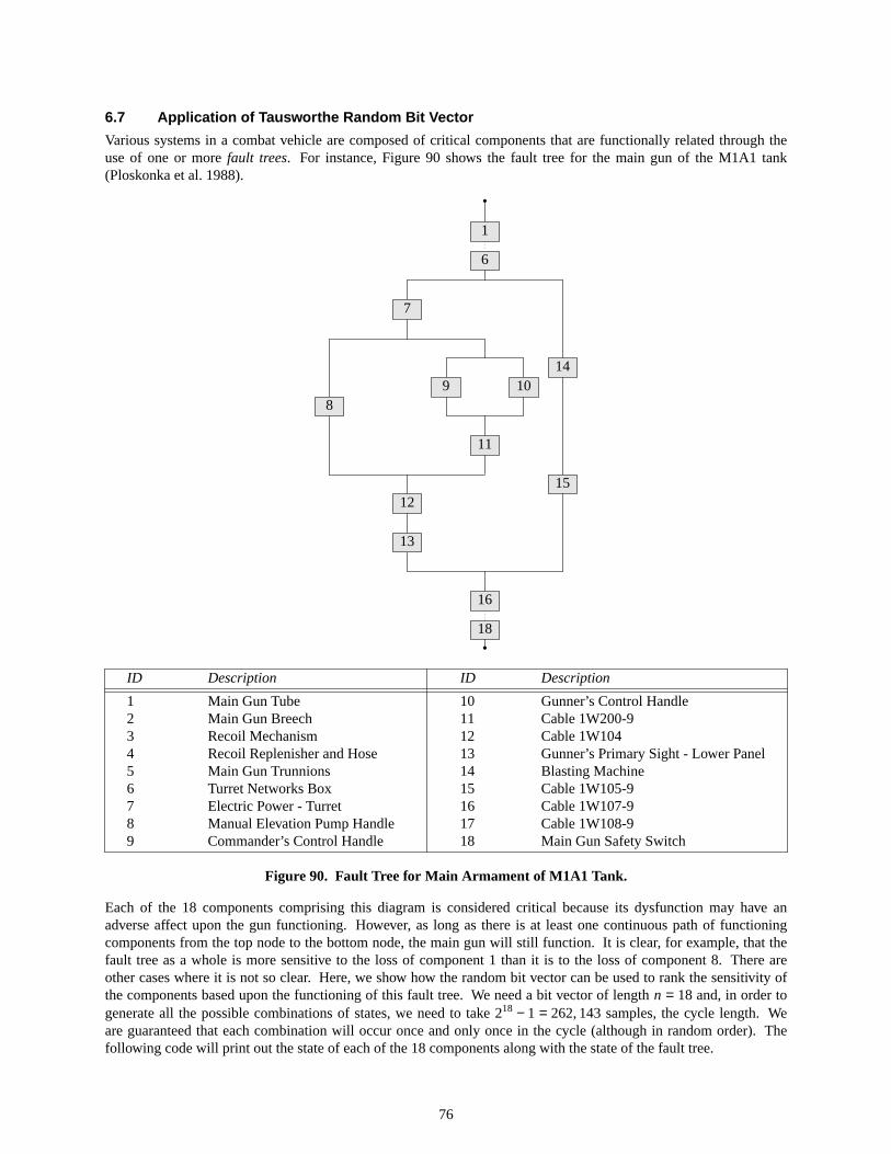
6.7 Application of Tausworthe Random Bit V ector
Various systems in a combat vehicle are composed of critical components that are functionally related through theuse of one or more fault trees. For instance, Figure 90 shows the fault tree for the main gun of the M1A1 tank(Ploskonka et al. 1988).
•
1
6
7
8
12
13
9 10
11
14
15
16
18•
ID Description ID Description
1 Main Gun Tube 10 Gunner’s Control Handle2 Main Gun Breech 11 Cable1W200-93 Recoil Mechanism 12 Cable1W1044 Recoil Replenisher and Hose 13 Gunner’s Primary Sight - Lower Panel5 Main Gun Trunnions 14 Blasting Machine6 Turret Networks Box 15 Cable1W105-97 Electric Power - Turret 16 Cable 1W107-98 Manual Elevation Pump Handle 17 Cable1W108-99 Commander’s Control Handle 18 Main Gun Safety Switch
Figure90. Fault Tree for Main Armament of M1A1 Tank.
Each of the 18 components comprising this diagram is considered critical because its dysfunction may have anadverse affect upon the gun functioning. However, as long as there is at least one continuous path of functioningcomponents from the top node to the bottom node, the main gun will still function. It is clear, for example, that thefault tree as a whole is more sensitive to the loss of component 1 than it is to the loss of component 8. There areother cases where it is not so clear. Here, we show how the random bit vector can be used to rank the sensitivity ofthe components based upon the functioning of this fault tree. We need a bit vector of length n = 18 and, in order togenerate all the possible combinations of states, we need to take 218 − 1 = 262, 143 samples, the cycle length. Weare guaranteed that each combination will occur once and only once in the cycle (although in random order). Thefollowing code will print out the state of each of the 18 components along with the state of the fault tree.
76
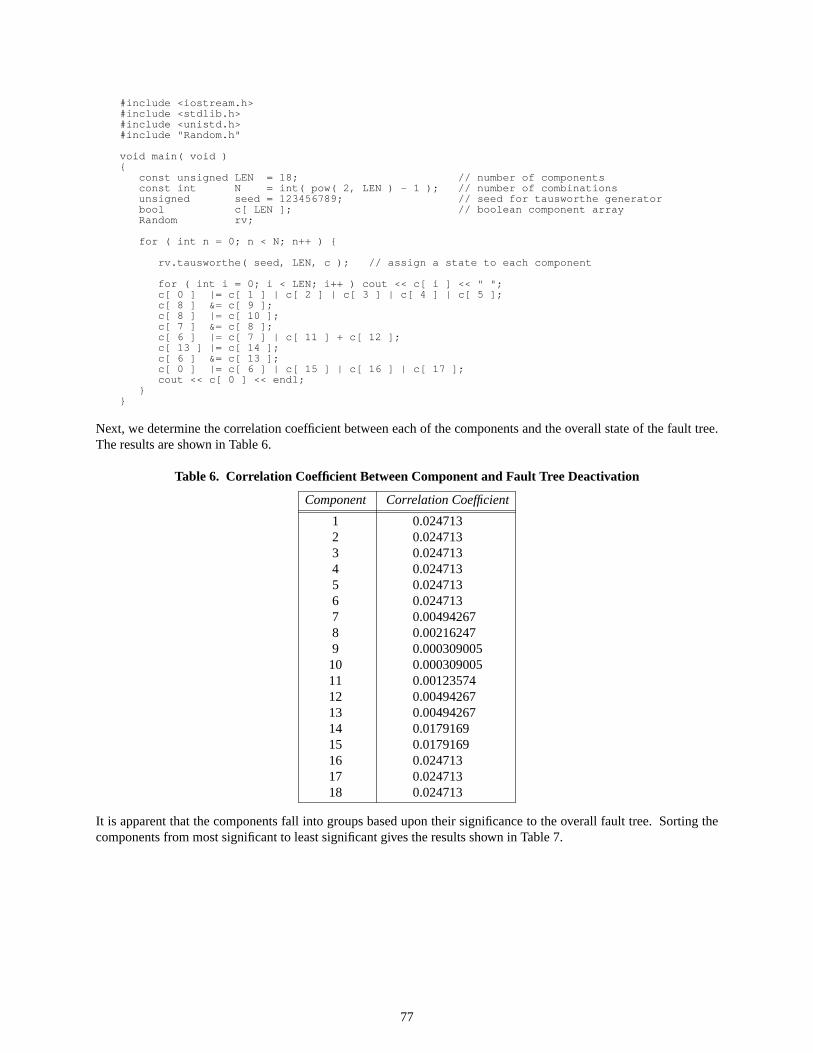
#include <iostream.h>#include <stdlib.h>#include <unistd.h>#include "Random.h"
void main( void ){
const unsigned LEN = 18; / / number of componentsconst int N = int( pow( 2, LEN ) - 1 ); // number of combinationsunsi gned seed = 123456789; / / seed for tausworthe generatorbool c[ LEN ]; // boolean component arrayRandom r v;
for ( int n = 0; n < N; n++ ) {
rv.tausworthe( seed, LEN, c ); // assign a state to each component
for ( int i = 0; i < LEN; i++ ) cout << c[ i ] << " ";c[ 0 ] |= c[ 1 ] | c[ 2 ] | c[ 3 ] | c[ 4 ] | c[ 5 ];c[ 8 ] &= c[ 9 ];c[ 8 ] |= c[ 10 ];c[ 7 ] &= c[ 8 ];c[ 6 ] |= c[ 7 ] | c[ 11 ] + c[ 12 ];c[ 13 ] |= c[ 14 ];c[ 6 ] &= c[ 13 ];c[ 0 ] |= c[ 6 ] | c[ 15 ] | c[ 16 ] | c[ 17 ];cout << c[ 0 ] << endl;
}}
Next, we determine the correlation coefficient between each of the components and the overall state of the fault tree.The results are shown in Table 6.
Table 6. Corr elation Coefficient Between Component and Fault TreeDeactivation
Component Correlation Coefficient
1 0.0247132 0.0247133 0.0247134 0.0247135 0.0247136 0.0247137 0.004942678 0.002162479 0.00030900510 0.00030900511 0.0012357412 0.0049426713 0.0049426714 0.017916915 0.017916916 0.02471317 0.02471318 0.024713
It is apparent that the components fall into groups based upon their significance to the overall fault tree. Sorting thecomponents from most significant to least significant gives the results shown in Table 7.
77

Table 7. Ranking of Component Significance to Fault TreeDeactivation
Group Components
1 1, 2, 3, 4, 5, 6, 16, 17, and 182 14 and 153 7, 12, and 134 85 116 9 and 10
This shows that components fall into six distinct classes based upon their significance to the overall fault tree. It alsogives a certain degree of verification that the coding is correct since it tell us that all the components in a given groupoccur in the fault tree with the same footing. It is clear by examing Figure 90 that components 7, 12, and 13, forinstance, all have the same significance to the vulnerability of the main gun.
Now, for the case shown here, where the number of components is 18, we could easily write a program consisting ofa series of nested loops to enumerate all 218 − 1 nonzero states. However, we do not have to add very many morecomponents before this direct enumeation approach will not be feasible. For instance, 30 components results inmore than one billion possible states. The Tausworthe random bit generator provides an alternative approach. Wecould replicate, say 100,000 times, knowing that the bit vectors will be unique as well as ‘‘random.’’ As such, it pro-vides a useful tool for the examination and verification of fault trees.
78
7. REFERENCES
Bodt, B. A., and M. S. Taylor. ‘‘A Data Based Random Number Generator for a Multivariate Distribution—AUser’s Manual.’’ ARBRL-TR-02439, U.S. Army Ballistic Research Laboratory, Aberdeen Proving Ground,MD, November 1982.
Diaconis, P., and B. Efron. ‘‘Computer-Intensive Methods in Statistics.’’ Scientific American, pp. 116–130, May,1983.
Efron, B., and R. Tibshirani. ‘‘Statistical Data Analysis in the Computer Age.’’ Science, pp. 390–395, 26 July 1991.
Hammersley, J. M., and D. C. Handscomb. Monte Carlo Methods. London: Methuen & Co. Ltd., 1967.
Hastings, N. A. J., and J. B. Peacock. Statistical Distributions: A Handbook for Students and Practitioners. NewYork: John Wiley & Sons, 1975.
Helicon Publishing.The Hutchinson Encyclopedia. http://www.helicon.co.uk, 1999.
Knuth, D. E. The Art of Computer Programming, Volume 2: Seminumerical Algorithms. London: Addison-Wesley,1969.
Law, A. M., and W. D. Kelton. Simulation Modeling and Analysis. New York: McGraw-Hill, Second Edition, 1991.
New York Times. New York, C1, C6, 8 November 1988.
Pitman, J.Probability. New York: Springer-Verlag, 1993.
Ploskonka, J. J., T. M. Muehl, and C. J. Dively. ‘‘Criticality Analysis of the M1A1 Tank.’’ BRL-MR-3671, U.S.Army Ballistic Research Laboratory, Aberdeen Proving Ground, MD, June 1988.
Press, W. H., S. A. Teukolsky, W. T. Vetterling, and B. P. Flannery. Numerical Recipes in C: The Art of ScientificComputing. New York: Cambridge University Press, Second Edition, 1992.
Ripley, B. D. Stochastic Simulation. New York: John Wiley & Sons, 1987.
Sachs, L.Applied Statistics:A Handbook of Techniques. New York: Springer-Verlag, Second Edition, 1984.
Spiegel, M. R. Probability and Statistics. New York: McGraw-Hill, 1975.
Tausworthe, R. C. ‘‘Random Numbers Generated by Linear Recurrence Modulo Two.’’ Mathematics ofComputation. Vol. 19, pp. 201–209, 1965.
Taylor, M. S., and J. R. Thompson. ‘‘A Data Based Algorithm for the Generation of Random Vectors.’’Computational Statistics & Data Analysis. Vol. 4, pp. 93–101, 1986.
Thompson, J. R.Empirical Model Building. New York: John Wiley & Sons, 1989.
Watson, E. J.‘‘Primitive Polynomials (Mod 2).’’ Mathematics of Computation. Vol. 16, pp. 368–369, 1962.
79

INTENTIONALLY LEFT BLANK.
80
APPENDIX A:UNIFORM RANDOM NUMBER GENERATOR
The underlying random number generator used is one that will generate uniformly distributed random numbers onthe half-open interval [0, 1). Any other distribution of random numbers, with few exceptions, results from mathe-matical transformation. Thus, it is clear that we need a good generator of random numbersU(0, 1). Here we discusssome criteria of what constitutes a good generator. After this, we discuss some tests that can be applied and showthe test results when applied to several candidate generators.
A.1 Selection Criteria
We will consider four attributes of what constitutes a good random number generator.
• RangeA good generator should have the capability of producing a large range of random numbers.
• SpeedA good generator should be fast.
• PortabilityThe generator should give the same sequence of random numbers, regardless of what computer it is run on.As a minimum, we need the explicit source code.
• ValidationA good generator should exhibit apparent randomness by passing certain well-accepted validation tests.
Six candidate generators were examined and tested for consideration as the underlying generator for U(0, 1). Theyare alllinear conguential generators of the form
Xi+1 = ( aXi + c ) ( modm). (A-1)
This is a recurrence relation for generating the next number in the sequence, given the multiplier a, the increment c,and the modulus m. The linear conguential method is a well-accepted technique for generating a sequence of num-bers that takeon the appearance of randomness.They possess the following properties.1,2
• They are relatively fast, requiring few arithmetic operations.
• They produce arangeof values no greater than the modulusm.
• They hav eaperiodor cycle lengthno greater thanm.
• Howev er, they are not free of sequential correlations.
We consider two generators available in standard C libraries, rand anddrand48 —and thus, commonly used—andfour versions of a generator proposed by Park and Miller.2,3 First, we give a short description of each one and list thesource code.
rand
This is the ANSI C version of a random number generator and has been implemented in C as follows:
unsigned long next = 1;
void srand( unsigned int seed ) /* set the seed */{
next = seed;}
int rand( void ) /* return a pseudo-random number */{
next = next * 1103515245 + 12345;return ( unsigned int )( next / 65536 ) % 32768;
}
1 Knuth, D. E. The Art of Computer Programming, Volume 2: Seminumerical Algorithms. London: Addison-Wesley, 1969.2 Press, W. H., S. A. Teukolsky, W. T. Vetterling, and B. P. Flannery. Numerical Recipes in C: The Art of Scientific Computing. New York:
Cambridge University Press, Second Edition, 1992.3 Park, S. K., and K. W. Miller. Communications of the ACM. Vol. 31, pp. 1192–1201, 1988.
81
Now, it may appear that the modulus here is 32,768, but, in fact, it is 232, due to the fact that ‘‘unsi gned l ong’’ is32 bits in length and so modulus 232 is implicit. However, due to the fact that the returned number is ‘‘% 32768 ’’ or‘‘modulo 32768’’ means that it is only capable of producing, at most, 32,768 distinct numbers. Thus, it has a periodof 232 and a range no greater than 32,768.
drand48
This also is in the standard C library. This generator uses three 16-bit integer words in order to perform 48-bit arith-metic. Theconstants area = 25, 214, 903, 917, c = 11, andm = 248, so that it thas a very long period.
// drand48.C: A portable implementation of drand48, this routine will/ / gener at e precisely the same stream of pseudo-random numbers/ / i n the interval [0,1) as drand48, for the same seed value./ / The drand48 algorithm is based on the linear congruential/ / x[ n + 1 ] = ( a * x[ n ] + c ) ( mod m ),/ / wher e/ / a = 25214903917 (0x5DEECE66D),/ / c = 11 ( 0xB), and/ / m = 2ˆ48 = 281474976710656 (0x1000000000000),/ / whi l e using 48-bit integer arithmetic, but ignoring/ / mul t i pl i cat i on and addition overflows of two 16-bit integers.
static const unsigned int N_BITS = 16;static const double TWO_16 = 1. / ( 1L << N_BITS );
static const unsigned int MASK = unsigned( 1 << ( N_BITS - 1 ) ) +unsigned( 1 << ( N_BITS - 1 ) ) - 1; // 65535
static const unsigned int X0 = 0x330E; / / 13070static const unsigned int X1 = 0xABCD; / / 43981static const unsigned int X2 = 0x1234; / / 4660static const unsigned int A0 = 0xE66D; / / 58989static const unsigned int A1 = 0xDEEC; / / 57068static const unsigned int A2 = 0x5; / / 5static const unsigned int C = 0xB; / / 11
static unsigned int x[ 3 ] = { X0, X1, X2 };static unsigned int a[ 3 ] = { A0, A1, A2 };static unsigned int c = C;
static void next( void );
void my_srand48( long seed ){
x[ 0 ] = X0;x[ 1 ] = unsigned( seed ) & MASK; // store low-order bitsx[ 2 ] = ( unsigned( seed ) >> N_BITS ) & MASK; // store high-order bitsa[ 0 ] = A0;a[ 1 ] = A1;a[ 2 ] = A2;c = C;
}
double drand48( void ){
next();return TWO_16 * ( TWO_16 * ( TWO_16 * x[ 0 ] + x[ 1 ] ) + x[ 2 ] );
}
static void next( void ){
unsigned p[ 2 ], q[ 2 ], r[ 2 ];bool car r y0, carry1, carry2;l ong pr od;
pr od = long( a[ 0 ] ) * long( x[ 0 ] );p[ 0 ] = unsigned( prod ) & MASK;p[ 1 ] = unsigned( prod >> N_BITS ) & MASK;
carry0 = long( p[ 0 ] ) + long( c ) > MASK;carry1 = long( p[ 1 ] ) + long( carry0 ) > MASK;p[ 0 ] = unsigned( p[ 0 ] + c ) & MASK;p[ 1 ] = unsigned( p[ 1 ] + carry0 ) & MASK;
pr od = long( a[ 0 ] ) * long( x[ 1 ] );q[ 0 ] = unsigned( prod ) & MASK;q[ 1 ] = unsigned( prod >> N_BITS ) & MASK;
82
carry0 = long( p[ 1 ] ) + long( q[ 0 ] ) > MASK;p[ 1 ] = unsigned( p[ 1 ] + q[ 0 ] ) & MASK;
pr od = long( a[ 1 ] ) * long( x[ 0 ] );r[ 0 ] = unsigned( prod ) & MASK;r[ 1 ] = unsigned( prod >> N_BITS ) & MASK;
carry2 = long( p[ 1 ] ) + long( r[ 0 ] ) > MASK;x[ 2 ] = unsigned( carry0 + carry1 + carry2 + q[ 1 ] + r[ 1 ] +
a[ 0 ] * x[ 2 ] + a[ 1 ] * x[ 1 ] +a[ 2 ] * x[ 0 ] ) & MASK;
x[ 1 ] = unsigned( p [ 1 ] + r[ 0 ] ) & MASK;x[ 0 ] = unsigned( p [ 0 ] ) & MASK;
}
ran0
This is the ‘‘minimal’’ random number generator of Park and Miller.3 The constants are a = 16, 807, c = 0, andm = 231 − 1 (a Mersenne prime). It uses Schrage’s method4 to implement the recurrence formula without overflowof a 32-bit word. It has a period of 231 − 2 = 2, 147, 483, 646.
// ran0.C: Minimal random number generator of Park and Miller./ / Ret ur ns a uniform random deviate in [0,1) with a period of 2ˆ31-2./ / Set or reset seed to any integer value (except the value 0) to/ / i ni t i al i ze the sequence; seed must not be altered between calls for/ / successi ve deviates in the sequence.// Ref: Press, W. H., et al., "Numerical Recipes in C", Cambridge, 1992, p. 278
#include <assert.h>
double ran0( long& seed ){
static const long M = 2147483647; / / Mersenne prime 2ˆ31-1static const long A = 16807; / / 7ˆ5 is a primitive root of Mstatic const long Q = 127773;static const long R = 2836;static const double F = 1. / M;
assert( seed != 0 ); // since it won’t work if seed = 0
long k = seed / Q; // compute seed = ( A * seed ) % Mseed = ( seed - k * Q ) * A - k * R; // without overflowif ( seed < 0 ) seed += M; // by Schrage’s method
return seed * F; // convert to a floating point}
ran1
This is the same as ran0 , with the same constants, but also makes use of Bays-Durham shuffle5 to break up sequen-tial correlations inherent in the linear congruential method.
// ran1.C: Random number generator of Park and Miller with Bays-Durham shuffle./ / Ret ur ns a uniform random deviate in [0,1) with a period of 2ˆ31-2./ / Set the seed to any integer value (except zero) to initialize the/ / sequence; seed must not be altered between calls for successive/ / devi at es in the sequence.// Ref: Press, W. H., et al., "Numerical Recipes in C", Cambridge, 1992, p. 278
#include <assert.h>
double ran1( long& seed ){
static const long M = 2147483647; / / Mersenne prime 2ˆ31-1static const long A = 16807; / / 7ˆ5 is a primitive root of Mstatic const long Q = 127773;static const long R = 2836;static const double F = 1. / M;static const short NTAB = 32;
3 Park, S. K., and K. W. Miller. Communications of the ACM. Vol. 31, pp. 1192–1201, 1988.4 Schrage, L.ACM Transactions on Mathematical Software. Vol. 5, pp. 132–138, 1979.5 Bays, C., and S. D. Durham. ‘‘ Improving a Poor Random Number Generator.’’ ACM Transactions on Mathematical Software, Vol. 2, pp.
59–64, 1976.
83
static const long DI V = 1 + ( M - 1 ) / NTAB;
assert( seed != 0 ); // since it won’t work if seed = 0
static long value = 0;static long table[ NTAB ];
if ( value == 0 ) { // load the shuffle table the first time through
for ( int i = NTAB + 7; i >= 0; i-- ) { // first perform 8 warm-ups
long k = seed / Q;seed = A * ( seed - k * Q ) - k * R;if ( seed < 0 ) seed += M;
if ( i < NTAB ) table[ i ] = seed;}value = table[ 0 ];
}
long k = seed / Q; // compute seed = ( A * seed ) % Mseed = A * ( seed - k * Q ) - k * R; // without overflowif ( seed < 0 ) seed += M; // by Schrage’s method
int i = value / DIV; // Bays-Durham shuffle algorithmvalue = table[ i ];table[ i ] = seed;
return value * F; // return a floating point}
ran1v2
This is version 2 ofran1 . It uses the multiplier, a = 48, 271.
// ran1v2.C: Random number generator of Park and Miller (version 2) with/ / Bays- Dur ham shuffle algorithm./ / Ret ur ns a uniform random deviate in [0,1) with a period of 2ˆ31-2./ / Set the seed to any integer value (except zero) to initialize the/ / sequence; seed must not be altered between calls for successive/ / devi at es in the sequence.// Ref: Press, W. H., et al., "Numerical Recipes in C", Cambridge, 1992, p. 278
#include <assert.h>
double ran1v2( long& seed ){
static const long M = 2147483647; / / Mersenne prime 2ˆ31-1static const long A = 48271; / / this is a prime numberstatic const long Q = 44488;static const long R = 3399;static const double F = 1. / M;static const short NTAB = 32;static const long DI V = 1 + ( M - 1 ) / NTAB;
assert( seed != 0 ); // since it won’t work if seed = 0
static long value = 0;static long table[ NTAB ];
if ( value == 0 ) { // load the shuffle table the first time through
for ( int i = NTAB + 7; i >= 0; i-- ) { // first perform 8 warm-ups
long k = seed / Q;seed = A * ( seed - k * Q ) - k * R;if ( seed < 0 ) seed += M;
if ( i < NTAB ) table[ i ] = seed;}value = table[ 0 ];
}
long k = seed / Q; // compute seed = ( A * seed ) % Mseed = A * ( seed - k * Q ) - k * R; // without overflowif ( seed < 0 ) seed += M; // by Schrage’s method
int i = value / DIV; // Bays-Durham shuffle algorithmvalue = table[ i ];
84
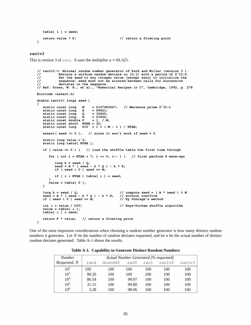
table[ i ] = seed;
return value * F; // return a floating point}
ran1v3
This is version 3 ofran1 . It uses the multipliera = 69, 621.
// ran1v3.C: Minimal random number generator of Park and Miller (version 3 )./ / Ret ur ns a uniform random deviate in [0,1) with a period of 2ˆ31-2./ / Set the seed to any integer value (except zero) to initialize the/ / sequence; seed must not be altered between calls for successive/ / devi at es in the sequence.// Ref: Press, W. H., et al., "Numerical Recipes in C", Cambridge, 1992, p. 278
#include <assert.h>
double ran1v3( long& seed ){
static const long M = 2147483647; / / Mersenne prime 2ˆ31-1static const long A = 69621;static const long Q = 30845;static const long R = 23902;static const double F = 1. / M;static const short NTAB = 32;static const long DI V = 1 + ( M - 1 ) / NTAB;
assert( seed != 0 ); // since it won’t work if seed = 0
static long value = 0;static long table[ NTAB ];
if ( value == 0 ) { // load the shuffle table the first time through
for ( int i = NTAB + 7; i >= 0; i-- ) { // first perform 8 warm-ups
long k = seed / Q;seed = A * ( seed - k * Q ) - k * R;if ( seed < 0 ) seed += M;
if ( i < NTAB ) table[ i ] = seed;}value = table[ 0 ];
}
long k = seed / Q; // compute seed = ( A * seed ) % Mseed = A * ( seed - k * Q ) - k * R; // without overflowif ( seed < 0 ) seed += M; // by Schrage’s method
int i = value / DIV; // Bays-Durham shuffle algorithmvalue = table[ i ];table[ i ] = seed;
return F * value; // return a floating point}
One of the most important considerations when choosing a random number generator is how many distinct randomnumbers it generates. Let N be the number of random deviates requested, and let n be the actual number of distinctrandom deviates generated.Table A-1 shows the results.
Table A-1. Capability to Generate Distinct Random Numbers
Number Actual Number Generated (% requested)Requested, N r and dr and48 r an0 r an1 r an1v2 r an1v3
102 100 100 100 100 100 100103 98.20 100 100 100 100 100104 86.54 100 99.97 100 100 100105 31.15 100 99.80 100 100 100106 3.28 100 98.06 100 100 100
85

It is not unreasonable to require 100,000 or more random numbers for a simulation, so these results alone should dis-qualify rand as a serious random number generator.
Next, let us compare the speed of the generators. Table A-2 shows the time to generate one million random deviateson a Silicon Graphics workstation with a 200–MHz processor.
Table A-2. Uniform Random Number Generator Timings
Number Computer Time (s)Requested, N r and dr and48 r an0 r an1 r an1v2 r an1v3
106 0.37 1.17 0.88 1.21 1.21 1.20
The relative timings are as follows.
rand : 1drand48 : 3.2ran0 : 2.4ran1 : 3.3ran1v2 : 3.3ran1v3 : 3.3
Although drand48 is over three times slower than rand , it is a much better generator. Also, as is apparent fromTable A-2, the computer time involved in generating uniform deviates is not likely to be a significant burden in asimulation.
Since we have the source code for all six of these generators, they all satisfy the portability requirement.
A.2 Validation T ests
Next, we subject the six candidate random number generators to four tests of randomness.
A.2.1 Chi-Square T est
The chi-square test is a check that the generated random numbers are distributed uniformly over the unit interval. Inorder to compute a value of χ 2 from our random number generators, we first subdivide the interval [0,1] into ksubintervals of equal length and then count the number ni that fall into the i th bin when a total of n random numbershave been generated.The computed value ofχ 2 is obtained from the formula
χ 2 =k
n
k
i =1Σ(ni − n/k)2, (A-2)
where
k is the number of bins,n is the total number of random deviates, andni is the number of random deviates in thei th bin.
As a general rule when carrying out this test, k should be at least 100 and n/k should be at least 5. As the number ofrandom samples, n, was increased, we increased the number of bins, k, such that the ratio n/k remained constant at8. Thecritical value ofχ 2 can be calculated with the aid of the formula, valid for largek,
χ 2k−1,1−α = (k − 1)
1 −
2
9(k − 1)+ z1−α √ 2/[9(k − 1)]
3
, (A-3)
where
k is the numbers of bins,α is the significance level, andz1−α is the 1− α critical point of the standard normal distribution, and has the value 1.645 whenα = 0. 05.
The results are displayed in Table A-3. (The seed used for all of these tests was 123456789.) All of the generatorsdo about the same until the number of bins exceeds 32,768. Beyond this point, rand completely fails the chi-square
86
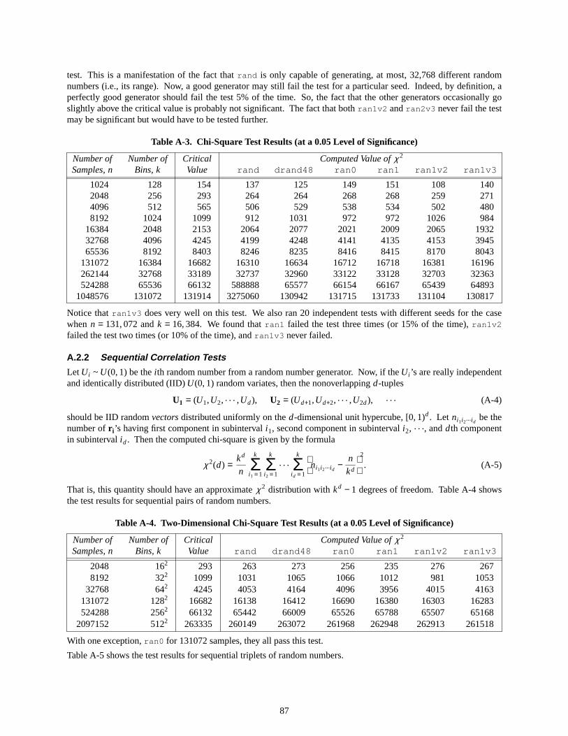
test. This is a manifestation of the fact that rand is only capable of generating, at most, 32,768 different randomnumbers (i.e., its range). Now, a good generator may still fail the test for a particular seed. Indeed, by definition, aperfectly good generator should fail the test 5% of the time. So, the fact that the other generators occasionally goslightly above the critical value is probably not significant. The fact that both ran1v2 andran2v3 never fail the testmay be significant but would have to be tested further.
Table A-3. Chi-SquareTest Results (at a 0.05 Level of Significance)
Number of Number of Critical Computed Value of χ 2
Samples, n Bins, k Value r and dr and48 r an0 r an1 r an1v2 r an1v3
1024 128 154 137 125 149 151 108 1402048 256 293 264 264 268 268 259 2714096 512 565 506 529 538 534 502 4808192 1024 1099 912 1031 972 972 1026 984
16384 2048 2153 2064 2077 2021 2009 2065 193232768 4096 4245 4199 4248 4141 4135 4153 394565536 8192 8403 8246 8235 8416 8415 8170 8043
131072 16384 16682 16310 16634 16712 16718 16381 16196262144 32768 33189 32737 32960 33122 33128 32703 32363524288 65536 66132 588888 65577 66154 66167 65439 64893
1048576 131072 131914 3275060 130942 131715 131733 131104 130817
Notice that ran1v3 does very well on this test. We also ran 20 independent tests with different seeds for the casewhen n = 131, 072 and k = 16, 384. We found that ran1 failed the test three times (or 15% of the time), ran1v2
failed the test two times (or 10% of the time), andran1v3 never failed.
A.2.2 Sequential Correlation T ests
Let Ui ~ U(0, 1) be the i th random number from a random number generator. Now, if theUi ’s are really independentand identically distributed (IID)U(0, 1) random variates, then the nonoverlappingd-tuples
U1 = (U1,U2, . . . ,Ud), U2 = (Ud+1,Ud+2, . . . ,U2d), . . . (A-4)
should be IID random vectors distributed uniformly on the d-dimensional unit hypercube, [0, 1)d. Let ni1i2...i dbe the
number of r i ’s having first component in subinterval i1, second component in subinterval i2, . . ., and dth componentin subinterval i d. Then the computed chi-square is given by the formula
χ 2(d) =kd
n
k
i1 =1Σ
k
i2 =1Σ . . .
k
i d =1Σ
ni1i2...i d
−n
kd
2
. (A-5)
That is, this quantity should have an approximateχ 2 distribution with kd − 1 degrees of freedom. Table A-4 showsthe test results for sequential pairs of random numbers.
Table A-4. Tw o-Dimensional Chi-SquareTest Results (at a 0.05 Level of Significance)
Number of Number of Critical Computed Value of χ 2
Samples, n Bins, k Value r and dr and48 r an0 r an1 r an1v2 r an1v3
2048 162 293 263 273 256 235 276 2678192 322 1099 1031 1065 1066 1012 981 1053
32768 642 4245 4053 4164 4096 3956 4015 4163131072 1282 16682 16138 16412 16690 16380 16303 16283524288 2562 66132 65442 66009 65526 65788 65507 65168
2097152 5122 263335 260149 263072 261968 262948 262913 261518
With one exception,ran0 for 131072 samples, they all pass this test.
Table A-5 shows the test results for sequential triplets of random numbers.
87
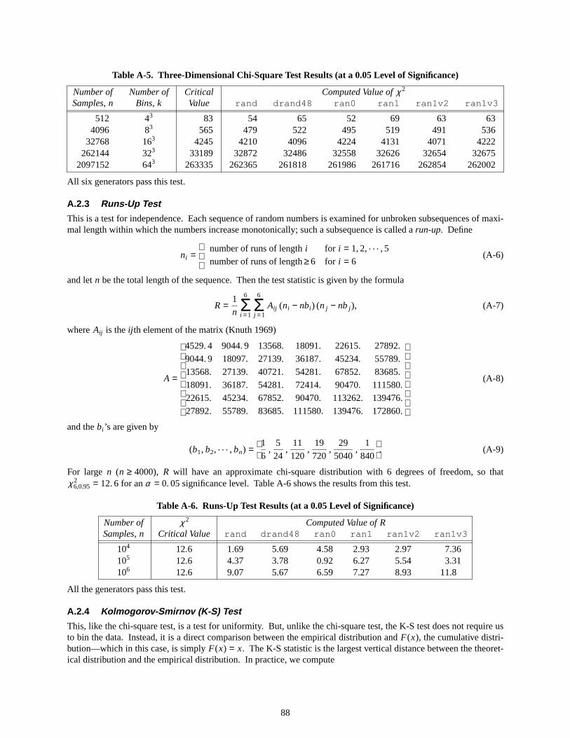
Table A-5. Thr ee-Dimensional Chi-SquareTest Results (at a 0.05 Level of Significance)
Number of Number of Critical Computed Value of χ 2
Samples, n Bins, k Value r and dr and48 r an0 r an1 r an1v2 r an1v3
512 43 83 54 65 52 69 63 634096 83 565 479 522 495 519 491 536
32768 163 4245 4210 4096 4224 4131 4071 4222262144 323 33189 32872 32486 32558 32626 32654 32675
2097152 643 263335 262365 261818 261986 261716 262854 262002
All six generators pass this test.
A.2.3 Runs-Up T est
This is a test for independence. Each sequence of random numbers is examined for unbroken subsequences of maxi-mal length within which the numbers increase monotonically; such a subsequence is called arun-up. Define
ni =
number of runs of lengthi
number of runs of length≥ 6
for i = 1, 2, . . . , 5
for i = 6(A-6)
and letn be the total length of the sequence.Then the test statistic is given by the formula
R =1
n
6
i =1Σ
6
j =1Σ Aij (ni − nbi ) (nj − nbj ), (A-7)
whereAij is theij th element of the matrix (Knuth 1969)
A =
4529. 4
9044. 9
13568.
18091.
22615.
27892.
9044. 9
18097.
27139.
36187.
45234.
55789.
13568.
27139.
40721.
54281.
67852.
83685.
18091.
36187.
54281.
72414.
90470.
111580.
22615.
45234.
67852.
90470.
113262.
139476.
27892.
55789.
83685.
111580.
139476.
172860.
(A-8)
and thebi ’s are given by
(b1, b2, . . . , bn) = 1
6,
5
24,
11
120,
19
720,
29
5040,
1
840. (A-9)
For large n (n ≥ 4000), R will have an approximate chi-square distribution with 6 degrees of freedom, so thatχ 2
6,0.95 = 12. 6 for anα = 0. 05 significance level. Table A-6 shows the results from this test.
Table A-6. Runs-Up Test Results (at a 0.05 Level of Significance)
Number of χ 2 Computed Value ofRSamples, n Critical Value r and dr and48 r an0 r an1 r an1v2 r an1v3
104 12.6 1.69 5.69 4.58 2.93 2.97 7.36105 12.6 4.37 3.78 0.92 6.27 5.54 3.31106 12.6 9.07 5.67 6.59 7.27 8.93 11.8
All the generators pass this test.
A.2.4 Kolmogor ov-Smirno v (K-S) Test
This, like the chi-square test, is a test for uniformity. But, unlike the chi-square test, the K-S test does not require usto bin the data. Instead, it is a direct comparison between the empirical distribution and F(x), the cumulative distri-bution—which in this case, is simply F(x) = x. The K-S statistic is the largest vertical distance between the theoret-ical distribution and the empirical distribution. In practice, we compute
88
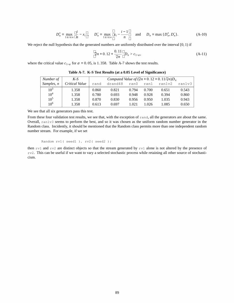
D+n =
1≤ i ≤ nmax
i
n− xi
, D−
n =1≤ i ≤ nmax
xi −
i − 1
n
and Dn = max { D+n, D−
n} . (A-10)
We reject the null hypothesis that the generated numbers are uniformly distributed over the interval [0,1) if
√
n + 0. 12 +0. 11
√ n
Dn > c1−α , (A-11)
where the critical valuec1−α for α = 0. 05, is 1.358. Table A-7 shows the test results.
Table A-7. K-S Test Results (at a 0.05 Level of Significance)
Number of K-S Computed Value of(√ n + 0. 12 + 0. 11/√ n)Dn
Samples, n Critical Value r and dr and48 r an0 r an1 r an1v2 r an1v3
103 1.358 0.860 0.821 0.794 0.700 0.651 0.543104 1.358 0.780 0.693 0.948 0.928 0.394 0.860105 1.358 0.870 0.830 0.956 0.950 1.035 0.943106 1.358 0.613 0.697 1.021 1.026 1.085 0.650
We see that all six generators pass this test.
From these four validation test results, we see that, with the exception of rand , all the generators are about the same.Overall, ran1v3 seems to perform the best, and so it was chosen as the uniform random number generator in theRandom class. Incidently, it should be mentioned that the Random class permits more than one independent randomnumber stream.For example, if we set
Random rv1( seed1 ), rv2( seed2 );
then rv1 and rv2 are distinct objects so that the stream generated by rv1 alone is not altered by the presence ofrv2 . This can be useful if we want to vary a selected stochastic process while retaining all other source of stochasti-cism.
89

INTENTIONALLY LEFT BLANK.
90
APPENDIX B:RANDOM CLASS SOURCE CODE
The definition and implementation of the Random class is consolidated into a single header file, Random.h . As aconsequence, it is only necessary to include this header file in any program that makes use of random number distri-butions. For example, here is a simple program that makes use of the Random class.
// Sample program for using the Random class
#include <iostream.h>#include "Random.h" ⇐ include the definition of the Random class
void main( void ){
Random rv; ⇐ declarea random variate
for ( int i = 0; i < 1000; i++ )cout << rv.normal() ⇐ reference the normal distribution (with default parameters)
<< endl;}
If this code is contained in the file main.C , then it can be compiled and linked into an executable program, main ,with the aid of the GNU C++ compiler by invoking the following UNIX command.
c++ -o main main.C -lm
This program will set the random number seed from the UNIX process ID. If we want to set the seed explicitly to123456789, simply make the following replacement.
Random rv; ⇒ Random rv( 123456789 );
If at any time later in the program we want to reset the seed, to say 773, we can do that with the following statement.
Random rv.reset( 773 );
The remaining pages of this appendix contain the complete source code of theRandomclass.
91

// Random.h: Definition and Implementation of Random Number Distribution Class// Ref: Richard Saucier, "Computer Generation of Statistical// Distributions," ARL-TR-2168, US Army Research Laboratory,// Aberdeen Proving Ground, MD, 21005-5068, March 2000.
#ifndef RANDOM_H#define RANDOM_H
#include <iostream>#include <fstream>#include <vector>#include <list>#include <algorithm>#include <functional>#include <cassert>#include <cmath>#include <cfloat> // for FLT_MIN and FLT_MAX#include <unistd.h> // for getpidusing namespace std;
// Constants for Tausworthe random bit generator// Ref: Tausworthe, Robert C., "Random Numbers Generated by Linear Recurrence// Modulo Two," Mathematics of Computation, vol. 19, pp. 201-209, 1965.
static const unsigned DEGREE_MAX = 32; // max degree (bits per word)
static const unsigned BIT[ 1 + DEGREE_MAX ] = {
// Hexidecimal Value Degree// ----------- ----- ------
0x00000000, // 0 00x00000001, // 2ˆ0 10x00000002, // 2ˆ1 20x00000004, // 2ˆ2 30x00000008, // 2ˆ3 40x00000010, // 2ˆ4 50x00000020, // 2ˆ5 60x00000040, // 2ˆ6 70x00000080, // 2ˆ7 80x00000100, // 2ˆ8 90x00000200, // 2ˆ9 100x00000400, // 2ˆ10 110x00000800, // 2ˆ11 120x00001000, // 2ˆ12 130x00002000, // 2ˆ13 140x00004000, // 2ˆ14 150x00008000, // 2ˆ15 160x00010000, // 2ˆ16 170x00020000, // 2ˆ17 180x00040000, // 2ˆ18 190x00080000, // 2ˆ19 200x00100000, // 2ˆ20 210x00200000, // 2ˆ21 220x00400000, // 2ˆ22 230x00800000, // 2ˆ23 240x01000000, // 2ˆ24 250x02000000, // 2ˆ25 260x04000000, // 2ˆ26 270x08000000, // 2ˆ27 280x10000000, // 2ˆ28 290x20000000, // 2ˆ29 300x40000000, // 2ˆ30 310x80000000 // 2ˆ31 32
};
// Coefficients that define a primitive polynomial (mod 2)// Ref: Watson, E. J., "Primitive Polynomials (Mod 2),"// Mathematics of Computation, vol. 16, pp. 368-369, 1962.
static const unsigned MASK[ 1 + DEGREE_MAX ] = {
BIT[0], // 0BIT[0], // 1BIT[1], // 2BIT[1], // 3BIT[1], // 4BIT[2], // 5BIT[1], // 6BIT[1], // 7BIT[4] + BIT[3] + BIT[2], // 8BIT[4], // 9BIT[3], // 10BIT[2], // 11BIT[6] + BIT[4] + BIT[1], // 12BIT[4] + BIT[3] + BIT[1], // 13BIT[5] + BIT[3] + BIT[1], // 14BIT[1], // 15BIT[5] + BIT[3] + BIT[2], // 16BIT[3], // 17BIT[5] + BIT[2] + BIT[1], // 18BIT[5] + BIT[2] + BIT[1], // 19BIT[3], // 20BIT[2], // 21
92
BIT[1], // 22BIT[5], // 23BIT[4] + BIT[3] + BIT[1], // 24BIT[3], // 25BIT[6] + BIT[2] + BIT[1], // 26BIT[5] + BIT[2] + BIT[1], // 27BIT[3], // 28BIT[2], // 29BIT[6] + BIT[4] + BIT[1], // 30BIT[3], // 31BIT[7] + BIT[5] + BIT[3] + BIT[2] + BIT[1] // 32
};
// for convenience, define some data structures for bivariate distributions
struct cartesianCoord { // cartesian coordinates in 2-D
double x, y;cartesianCoord& operator+=( const cartesianCoord& p ) {
x += p.x;y += p.y;return *this;
}cartesianCoord& operator-=( const cartesianCoord& p ) {
x -= p.x;y -= p.y;return *this;
}cartesianCoord& operator*=( double scalar ) {
x *= scalar;y *= scalar;return *this;
}cartesianCoord& operator/=( double scalar ) {
x /= scalar;y /= scalar;return *this;
}};
struct sphericalCoord { // spherical coordinates on unit sphere
double theta, phi;double x( void ) { return sin( theta ) * cos( phi ); } // x-coordinatedouble y( void ) { return sin( theta ) * sin( phi ); } // y-coordinatedouble z( void ) { return cos( theta ); } // z-coordinate
};
class Random {
// friends list// overloaded relational operators
friend bool operator==( const Random& p, const Random& q ){
bool equal = ( p._seed == q._seed ) && ( p._next == q._next );for ( int i = 0; i < p._NTAB; i++ )
equal = equal && ( p._table[ i ] == q._table[ i ] );return equal;
}
friend bool operator!=( const Random& p, const Random& q ){
return !( p == q );}
// overloaded stream operator
friend istream& operator>>( istream& is, Random& rv ){
cout << "Enter a random number seed "<< "(between 1 and " << LONG_MAX - 1 << ", inclusive): " << endl;
is >> rv._seed;
assert( rv._seed != 0 && rv._seed != LONG_MAX );
rv._seedTable();
return is;}
public:
Random( long seed ) // constructor to set the seed{
assert( seed != 0 && seed != LONG_MAX );_seed = seed;_seedTable();
_seed2 = _seed | 1; // for tausworthe random bit generation}
93
Random( void ) // default constructor uses process id to set the seed{
_seed = long( getpid() );_seedTable();_seed2 = _seed | 1; // for tausworthe random bit generation
}
˜Random( void ) // default destructor{}
Random( const Random& r ) // copy constructor (copies current state){
_seed = r._seed;_seed2 = r._seed2;
// copy the current state of the shuffle table
_next = r._next;for ( int i = 0; i < _NTAB; i++ ) _table[ i ] = r._table[ i ];
}
Random& operator=( const Random& r ) // overloaded assignment{
if ( *this == r ) return *this;
_seed = r._seed;_seed2 = r._seed2;
// copy the current state of the shuffle table
_next = r._next;for ( int i = 0; i < _NTAB; i++ ) _table[ i ] = r._table[ i ];
return *this;}
// utility functions
void reset( long seed ) // reset the seed explicitly{
assert( seed != 0 && seed != LONG_MAX );_seed = seed;_seedTable();_seed2 = _seed | 1; // so that all bits cannot be zero
}
void reset( void ) // reset seed from current process id{
_seed = long( getpid() );_seedTable();_seed2 = _seed | 1; // so that all bits cannot be zero
}
// Continuous Distributions
double arcsine( double xMin = 0., double xMax = 1. ) // Arc Sine{
double q = sin( M_PI_2 * _u() );return xMin + ( xMax - xMin ) * q * q;
}
double beta( double v, double w, // Betadouble xMin = 0., double xMax = 1. ) // (v > 0. and w > 0.)
{if ( v < w ) return xMax - ( xMax - xMin ) * beta( w, v );double y1 = gamma( 0., 1., v );double y2 = gamma( 0., 1., w );return xMin + ( xMax - xMin ) * y1 / ( y1 + y2 );
}
double cauchy( double a = 0., double b = 1. ) // Cauchy (or Lorentz){
// a is the location parameter and b is the scale parameter// b is the half width at half maximum (HWHM) and variance doesn’t exist
assert( b > 0. );
return a + b * tan( M_PI * uniform( -0.5, 0.5 ) );}
double chiSquare( int df ) // Chi-Square{
assert( df >= 1 );
return gamma( 0., 2., 0.5 * double( df ) );}
double cosine( double xMin = 0., double xMax = 1. ) // Cosine{
assert( xMin < xMax );
double a = 0.5 * ( xMin + xMax ); // location parameter
94
double b = ( xMax - xMin ) / M_PI; // scale parameter
return a + b * asin( uniform( -1., 1. ) );}
double doubleLog( double xMin = -1., double xMax = 1. ) // Double Log{
assert( xMin < xMax );
double a = 0.5 * ( xMin + xMax ); // location parameterdouble b = 0.5 * ( xMax - xMin ); // scale parameter
if ( bernoulli( 0.5 ) ) return a + b * _u() * _u();else return a - b * _u() * _u();
}
double erlang( double b, int c ) // Erlang (b > 0. and c >= 1){
assert( b > 0. && c >= 1 );
double prod = 1.;for ( int i = 0; i < c; i++ ) prod *= _u();
return -b * log( prod );}
double exponential( double a = 0., double c = 1. ) // Exponential{ // location a, shape c
assert( c > 0.0 );
return a - c * log( _u() );}
double extremeValue( double a = 0., double c = 1. ) // Extreme Value{ // location a, shape c
assert( c > 0. );
return a + c * log( -log( _u() ) );}
double fRatio( int v, int w ) // F Ratio (v and w >= 1){
assert( v >= 1 && w >= 1 );
return ( chiSquare( v ) / v ) / ( chiSquare( w ) / w );}
double gamma( double a, double b, double c ) // Gamma{ // location a, scale b, shape c
assert( b > 0. && c > 0. );
const double A = 1. / sqrt( 2. * c - 1. );const double B = c - log( 4. );const double Q = c + 1. / A;const double T = 4.5;const double D = 1. + log( T );const double C = 1. + c / M_E;
if ( c < 1. ) {while ( true ) {
double p = C * _u();if ( p > 1. ) {
double y = -log( ( C - p ) / c );if ( _u() <= pow( y, c - 1. ) ) return a + b * y;
}else {
double y = pow( p, 1. / c );if ( _u() <= exp( -y ) ) return a + b * y;
}}
}else if ( c == 1.0 ) return exponential( a, b );else {
while ( true ) {double p1 = _u();double p2 = _u();double v = A * log( p1 / ( 1. - p1 ) );double y = c * exp( v );double z = p1 * p1 * p2;double w = B + Q * v - y;if ( w + D - T * z >= 0. || w >= log( z ) ) return a + b * y;
}}
}
double laplace( double a = 0., double b = 1. ) // Laplace{ // (or double exponential)
assert( b > 0. );
// composition method
if ( bernoulli( 0.5 ) ) return a + b * log( _u() );else return a - b * log( _u() );
95
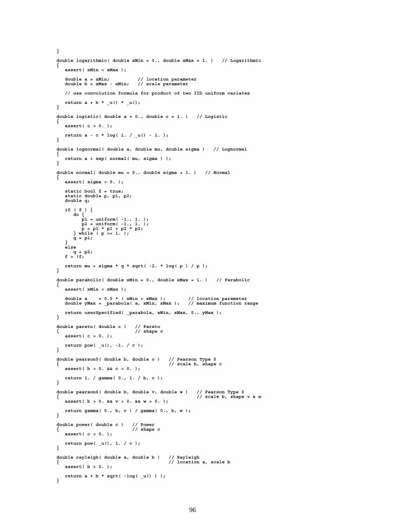
}
double logarithmic( double xMin = 0., double xMax = 1. ) // Logarithmic{
assert( xMin < xMax );
double a = xMin; // location parameterdouble b = xMax - xMin; // scale parameter
// use convolution formula for product of two IID uniform variates
return a + b * _u() * _u();}
double logistic( double a = 0., double c = 1. ) // Logistic{
assert( c > 0. );
return a - c * log( 1. / _u() - 1. );}
double lognormal( double a, double mu, double sigma ) // Lognormal{
return a + exp( normal( mu, sigma ) );}
double normal( double mu = 0., double sigma = 1. ) // Normal{
assert( sigma > 0. );
static bool f = true;static double p, p1, p2;double q;
if ( f ) {do {
p1 = uniform( -1., 1. );p2 = uniform( -1., 1. );p = p1 * p1 + p2 * p2;
} while ( p >= 1. );q = p1;
}else
q = p2;f = !f;
return mu + sigma * q * sqrt( -2. * log( p ) / p );}
double parabolic( double xMin = 0., double xMax = 1. ) // Parabolic{
assert( xMin < xMax );
double a = 0.5 * ( xMin + xMax ); // location parameterdouble yMax = _parabola( a, xMin, xMax ); // maximum function range
return userSpecified( _parabola, xMin, xMax, 0., yMax );}
double pareto( double c ) // Pareto{ // shape c
assert( c > 0. );
return pow( _u(), -1. / c );}
double pearson5( double b, double c ) // Pearson Type 5{ // scale b, shape c
assert( b > 0. && c > 0. );
return 1. / gamma( 0., 1. / b, c );}
double pearson6( double b, double v, double w ) // Pearson Type 6{ // scale b, shape v & w
assert( b > 0. && v > 0. && w > 0. );
return gamma( 0., b, v ) / gamma( 0., b, w );}
double power( double c ) // Power{ // shape c
assert( c > 0. );
return pow( _u(), 1. / c );}
double rayleigh( double a, double b ) // Rayleigh{ // location a, scale b
assert( b > 0. );
return a + b * sqrt( -log( _u() ) );}
96
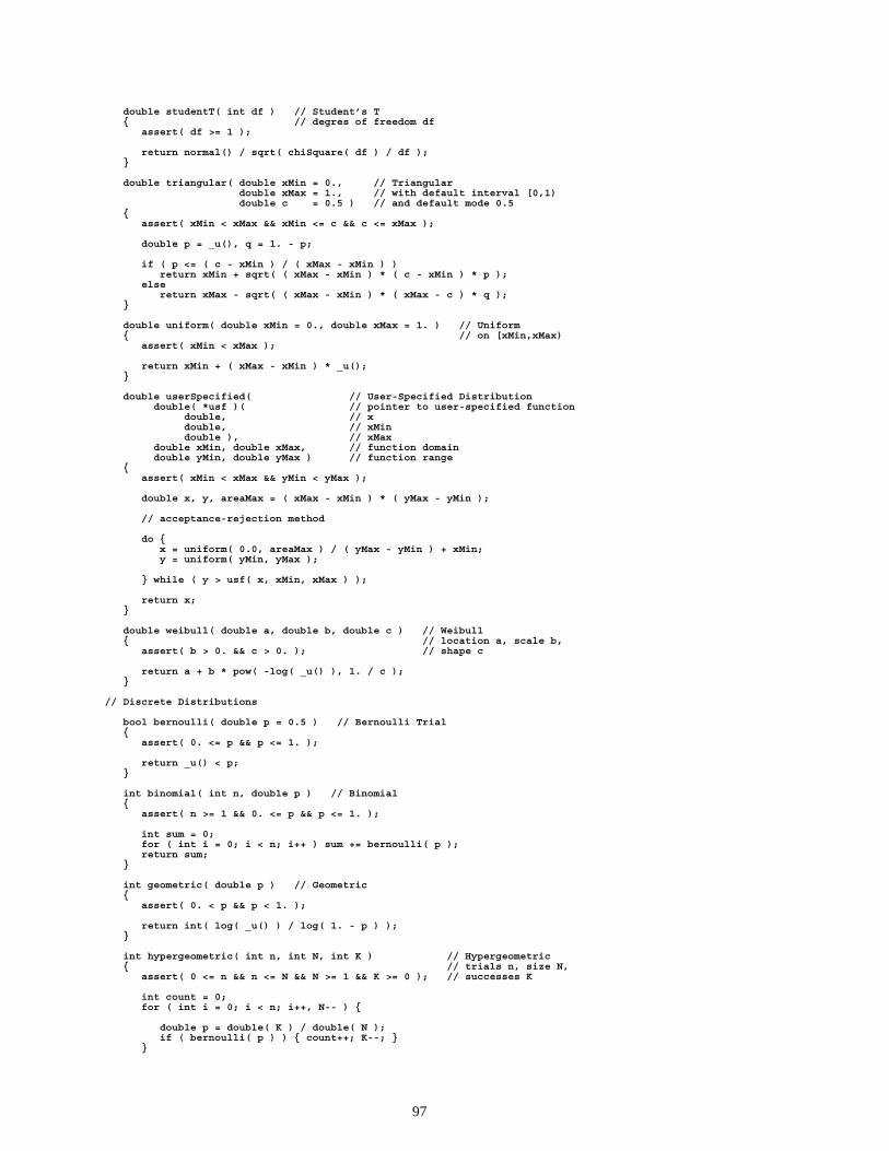
double studentT( int df ) // Student’s T{ // degres of freedom df
assert( df >= 1 );
return normal() / sqrt( chiSquare( df ) / df );}
double triangular( double xMin = 0., // Triangulardouble xMax = 1., // with default interval [0,1)double c = 0.5 ) // and default mode 0.5
{assert( xMin < xMax && xMin <= c && c <= xMax );
double p = _u(), q = 1. - p;
if ( p <= ( c - xMin ) / ( xMax - xMin ) )return xMin + sqrt( ( xMax - xMin ) * ( c - xMin ) * p );
elsereturn xMax - sqrt( ( xMax - xMin ) * ( xMax - c ) * q );
}
double uniform( double xMin = 0., double xMax = 1. ) // Uniform{ // on [xMin,xMax)
assert( xMin < xMax );
return xMin + ( xMax - xMin ) * _u();}
double userSpecified( // User-Specified Distributiondouble( *usf )( // pointer to user-specified function
double, // xdouble, // xMindouble ), // xMax
double xMin, double xMax, // function domaindouble yMin, double yMax ) // function range
{assert( xMin < xMax && yMin < yMax );
double x, y, areaMax = ( xMax - xMin ) * ( yMax - yMin );
// acceptance-rejection method
do {x = uniform( 0.0, areaMax ) / ( yMax - yMin ) + xMin;y = uniform( yMin, yMax );
} while ( y > usf( x, xMin, xMax ) );
return x;}
double weibull( double a, double b, double c ) // Weibull{ // location a, scale b,
assert( b > 0. && c > 0. ); // shape c
return a + b * pow( -log( _u() ), 1. / c );}
// Discrete Distributions
bool bernoulli( double p = 0.5 ) // Bernoulli Trial{
assert( 0. <= p && p <= 1. );
return _u() < p;}
int binomial( int n, double p ) // Binomial{
assert( n >= 1 && 0. <= p && p <= 1. );
int sum = 0;for ( int i = 0; i < n; i++ ) sum += bernoulli( p );return sum;
}
int geometric( double p ) // Geometric{
assert( 0. < p && p < 1. );
return int( log( _u() ) / log( 1. - p ) );}
int hypergeometric( int n, int N, int K ) // Hypergeometric{ // trials n, size N,
assert( 0 <= n && n <= N && N >= 1 && K >= 0 ); // successes K
int count = 0;for ( int i = 0; i < n; i++, N-- ) {
double p = double( K ) / double( N );if ( bernoulli( p ) ) { count++; K--; }
}
97
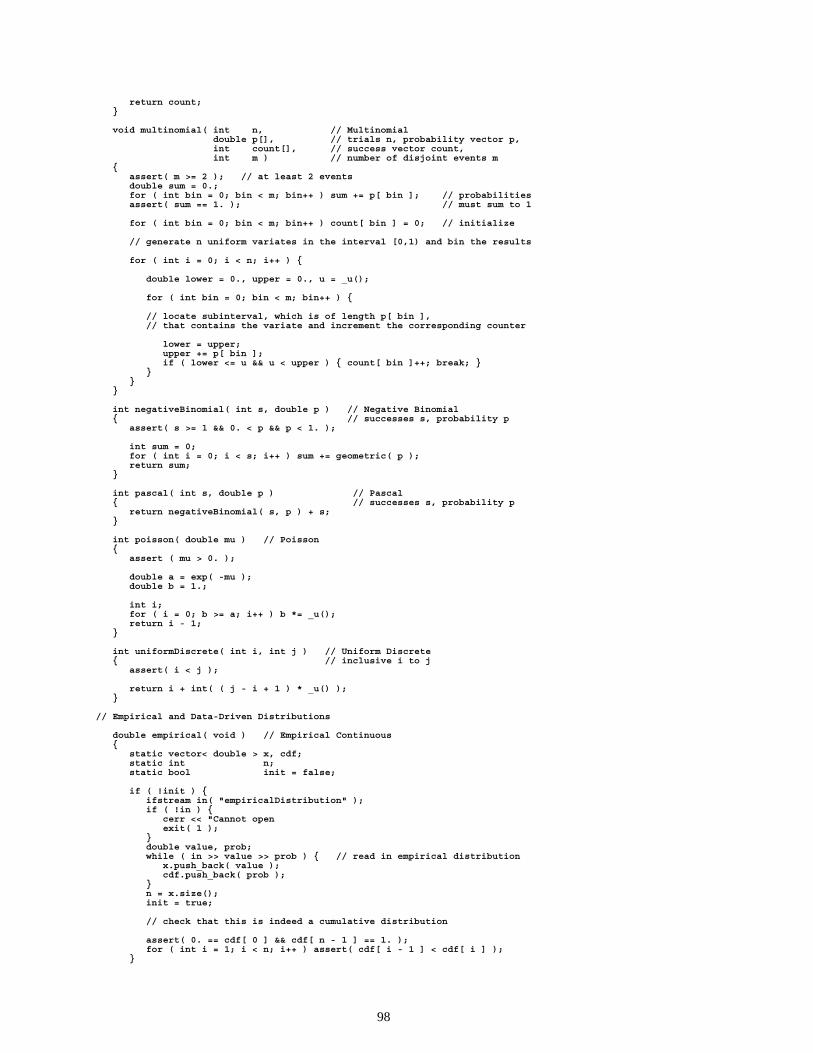
return count;}
void multinomial( int n, // Multinomialdouble p[], // trials n, probability vector p,int count[], // success vector count,int m ) // number of disjoint events m
{assert( m >= 2 ); // at least 2 eventsdouble sum = 0.;for ( int bin = 0; bin < m; bin++ ) sum += p[ bin ]; // probabilitiesassert( sum == 1. ); // must sum to 1
for ( int bin = 0; bin < m; bin++ ) count[ bin ] = 0; // initialize
// generate n uniform variates in the interval [0,1) and bin the results
for ( int i = 0; i < n; i++ ) {
double lower = 0., upper = 0., u = _u();
for ( int bin = 0; bin < m; bin++ ) {
// locate subinterval, which is of length p[ bin ],// that contains the variate and increment the corresponding counter
lower = upper;upper += p[ bin ];if ( lower <= u && u < upper ) { count[ bin ]++; break; }
}}
}
int negativeBinomial( int s, double p ) // Negative Binomial{ // successes s, probability p
assert( s >= 1 && 0. < p && p < 1. );
int sum = 0;for ( int i = 0; i < s; i++ ) sum += geometric( p );return sum;
}
int pascal( int s, double p ) // Pascal{ // successes s, probability p
return negativeBinomial( s, p ) + s;}
int poisson( double mu ) // Poisson{
assert ( mu > 0. );
double a = exp( -mu );double b = 1.;
int i;for ( i = 0; b >= a; i++ ) b *= _u();return i - 1;
}
int uniformDiscrete( int i, int j ) // Uniform Discrete{ // inclusive i to j
assert( i < j );
return i + int( ( j - i + 1 ) * _u() );}
// Empirical and Data-Driven Distributions
double empirical( void ) // Empirical Continuous{
static vector< double > x, cdf;static int n;static bool init = false;
if ( !init ) {ifstream in( "empiricalDistribution" );if ( !in ) {
cerr << "Cannot openexit( 1 );
}double value, prob;while ( in >> value >> prob ) { // read in empirical distribution
x.push_back( value );cdf.push_back( prob );
}n = x.size();init = true;
// check that this is indeed a cumulative distribution
assert( 0. == cdf[ 0 ] && cdf[ n - 1 ] == 1. );for ( int i = 1; i < n; i++ ) assert( cdf[ i - 1 ] < cdf[ i ] );
}
98
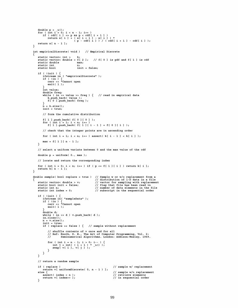
double p = _u();for ( int i = 0; i < n - 1; i++ )
if ( cdf[ i ] <= p && p < cdf[ i + 1 ] )return x[ i ] + ( x[ i + 1 ] - x[ i ] ) *
( p - cdf[ i ] ) / ( cdf[ i + 1 ] - cdf[ i ] );return x[ n - 1 ];
}
int empiricalDiscrete( void ) // Empirical Discrete{
static vector< int > k;static vector< double > f[ 2 ]; // f[ 0 ] is pdf and f[ 1 ] is cdfstatic double max;static int n;static bool init = false;
if ( !init ) {ifstream in ( "empiricalDiscrete" );if ( !in ) {
cerr << "Cannot openexit( 1 );
}int value;double freq;while ( in >> value >> freq ) { // read in empirical data
k.push_back( value );f[ 0 ].push_back( freq );
}n = k.size();init = true;
// form the cumulative distribution
f[ 1 ].push_back( f[ 0 ][ 0 ] );for ( int i = 1; i < n; i++ )
f[ 1 ].push_back( f[ 1 ][ i - 1 ] + f[ 0 ][ i ] );
// check that the integer points are in ascending order
for ( int i = 1; i < n; i++ ) assert( k[ i - 1 ] < k[ i ] );
max = f[ 1 ][ n - 1 ];}
// select a uniform variate between 0 and the max value of the cdf
double p = uniform( 0., max );
// locate and return the corresponding index
for ( int i = 0; i < n; i++ ) if ( p <= f[ 1 ][ i ] ) return k[ i ];return k[ n - 1 ];
}
double sample( bool replace = true ) // Sample w or w/o replacement from a{ // distribution of 1-D data in a file
static vector< double > v; // vector for sampling with replacementstatic bool init = false; // flag that file has been read instatic int n; // number of data elements in the filestatic int index = 0; // subscript in the sequential order
if ( !init ) {ifstream in( "sampleData" );if ( !in ) {
cerr << "Cannot openexit( 1 );
}double d;while ( in >> d ) v.push_back( d );in.close();n = v.size();init = true;if ( replace == false ) { // sample without replacement
// shuffle contents of v once and for all// Ref: Knuth, D. E., The Art of Computer Programming, Vol. 2:// Seminumerical Algorithms. London: Addison-Wesley, 1969.
for ( int i = n - 1; i > 0; i-- ) {int j = int( ( i + 1 ) * _u() );swap( v[ i ], v[ j ] );
}}
}
// return a random sample
if ( replace ) // sample w/ replacementreturn v[ uniformDiscrete( 0, n - 1 ) ];
else { // sample w/o replacementassert( index < n ); // retrieve elementsreturn v[ index++ ]; // in sequential order
}
99
}
void sample( double x[], int ndim ) // Sample from a given distribution{ // of multi-dimensional data
static const int N_DIM = 6;assert( ndim <= N_DIM );
static vector< double > v[ N_DIM ];static bool init = false;static int n;
if ( !init ) {ifstream in( "sampleData" );if ( !in ) {
cerr << "Cannot openexit( 1 );
}double d;while ( !in.eof() ) {
for ( int i = 0; i < ndim; i++ ) {in >> d;v[ i ].push_back( d );
}}in.close();n = v[ 0 ].size();init = true;
}int index = uniformDiscrete( 0, n - 1 );for ( int i = 0; i < ndim; i++ ) x[ i ] = v[ i ][ index ];
}
// comparison functor for determining the neighborhood of a data point
struct dSquared :public binary_function< cartesianCoord, cartesianCoord, bool > {
bool operator()( cartesianCoord p, cartesianCoord q ) {return p.x * p.x + p.y * p.y < q.x * q.x + q.y * q.y;
}};
cartesianCoord stochasticInterpolation( void ) // Stochastic Interpolation
// Refs: Taylor, M. S. and J. R. Thompson, Computational Statistics & Data// Analysis, Vol. 4, pp. 93-101, 1986; Thompson, J. R., Empirical Model// Building, pp. 108-114, Wiley, 1989; Bodt, B. A. and M. S. Taylor,// A Data Based Random Number Generator for A Multivariate Distribution// - A User’s Manual, ARBRL-TR-02439, BRL, APG, MD, Nov. 1982.{
static vector< cartesianCoord > data;static cartesianCoord min, max;static int m;static double lower, upper;static bool init = false;
if ( !init ) {ifstream in( "stochasticData" );if ( !in ) {
cerr << "Cannot openexit( 1 );
}
// read in the data and set min and max values
min.x = min.y = FLT_MAX;max.x = max.y = FLT_MIN;cartesianCoord p;while ( in >> p.x >> p.y ) {
min.x = ( p.x < min.x ? p.x : min.x );min.y = ( p.y < min.y ? p.y : min.y );max.x = ( p.x > max.x ? p.x : max.x );max.y = ( p.y > max.y ? p.y : max.y );
data.push_back( p );}in.close();init = true;
// scale the data so that each dimension will have equal weight
for ( int i = 0; i < data.size(); i++ ) {
data[ i ].x = ( data[ i ].x - min.x ) / ( max.x - min.x );data[ i ].y = ( data[ i ].y - min.y ) / ( max.y - min.y );
}
// set m, the number of points in a neighborhood of a given point
m = data.size() / 20; // 5% of all the data pointsif ( m < 5 ) m = 5; // but no less than 5if ( m > 20 ) m = 20; // and no more than 20
100
lower = ( 1. - sqrt( 3. * ( double( m ) - 1. ) ) ) / double( m );upper = ( 1. + sqrt( 3. * ( double( m ) - 1. ) ) ) / double( m );
}
// uniform random selection of a data point (with replacement)
cartesianCoord origin = data[ uniformDiscrete( 0, data.size() - 1 ) ];
// make this point the origin of the coordinate system
for ( int n = 0; n < data.size(); n++ ) data[ n ] -= origin;
// sort the data with respect to its distance (squared) from this origin
sort( data.begin(), data.end(), dSquared() );
// find the mean value of the data in the neighborhood about this point
cartesianCoord mean;mean.x = mean.y = 0.;for ( int n = 0; n < m; n++ ) mean += data[ n ];mean /= double( m );
// select a random linear combination of the points in this neighborhood
cartesianCoord p;p.x = p.y = 0.;for ( int n = 0; n < m; n++ ) {
double rn;if ( m == 1 ) rn = 1.;else rn = uniform( lower, upper );p.x += rn * ( data[ n ].x - mean.x );p.y += rn * ( data[ n ].y - mean.y );
}
// restore the data to its original form
for ( int n = 0; n < data.size(); n++ ) data[ n ] += origin;
// use mean and original point to translate the randomly-chosen point
p += mean;p += origin;
// scale randomly-chosen point to the dimensions of the original data
p.x = p.x * ( max.x - min.x ) + min.x;p.y = p.y * ( max.y - min.y ) + min.y;
return p;}
// Multivariate Distributions
cartesianCoord bivariateNormal( double muX = 0., // Bivariate Gaussiandouble sigmaX = 1.,double muY = 0.,double sigmaY = 1. )
{assert( sigmaX > 0. && sigmaY > 0. );
cartesianCoord p;p.x = normal( muX, sigmaX );p.y = normal( muY, sigmaY );return p;
}
cartesianCoord bivariateUniform( double xMin = -1., // Bivariate Uniformdouble xMax = 1.,double yMin = -1.,double yMax = 1. )
{assert( xMin < xMax && yMin < yMax );
double x0 = 0.5 * ( xMin + xMax );double y0 = 0.5 * ( yMin + yMax );double a = 0.5 * ( xMax - xMin );double b = 0.5 * ( yMax - yMin );double x, y;
do {x = uniform( -1., 1. );y = uniform( -1., 1. );
} while( x * x + y * y > 1. );
cartesianCoord p;p.x = x0 + a * x;p.y = y0 + b * y;return p;
}
101

cartesianCoord corrNormal( double r, // Correlated Normaldouble muX = 0.,double sigmaX = 1.,double muY = 0.,double sigmaY = 1. )
{assert( -1. <= r && r <= 1. && // bounds on correlation coeff
sigmaX > 0. && sigmaY > 0. ); // positive std dev
double x = normal();double y = normal();
y = r * x + sqrt( 1. - r * r ) * y; // correlate the variables
cartesianCoord p;p.x = muX + sigmaX * x; // translate and scalep.y = muY + sigmaY * y;return p;
}
cartesianCoord corrUniform( double r, // Correlated Uniformdouble xMin = 0.,double xMax = 1.,double yMin = 0.,double yMax = 1. )
{assert( -1. <= r && r <= 1. && // bounds on correlation coeff
xMin < xMax && yMin < yMax ); // bounds on domain
double x0 = 0.5 * ( xMin + xMax );double y0 = 0.5 * ( yMin + yMax );double a = 0.5 * ( xMax - xMin );double b = 0.5 * ( yMax - yMin );double x, y;
do {x = uniform( -1., 1. );y = uniform( -1., 1. );
} while ( x * x + y * y > 1. );
y = r * x + sqrt( 1. - r * r ) * y; // correlate the variables
cartesianCoord p;p.x = x0 + a * x; // translate and scalep.y = y0 + b * y;return p;
}
sphericalCoord spherical( double thMin = 0., // Uniform Sphericaldouble thMax = M_PI,double phMin = 0.,double phMax = 2. * M_PI )
{assert( 0. <= thMin && thMin < thMax && thMax <= M_PI &&
0. <= phMin && phMin < phMax && phMax <= 2. * M_PI );
sphericalCoord p; // azimuthp.theta = acos( uniform( cos( thMax ), cos( thMin ) ) ); // polar anglep.phi = uniform( phMin, phMax ); // azimuthreturn p;
}
void sphericalND( double x[], int n ) // Uniform over the surface of// an n-dimensional unit sphere
{// generate a point inside the unit n-sphere by normal polar method
double r2 = 0.;for ( int i = 0; i < n; i++ ) {
x[ i ] = normal();r2 += x[ i ] * x[ i ];
}
// project the point onto the surface of the unit n-sphere by scaling
const double A = 1. / sqrt( r2 );for ( int i = 0; i < n; i++ ) x[ i ] *= A;
}
// Number Theoretic Distributions
double avoidance( void ) // Maximal Avoidance (1-D){ // overloaded for convenience
double x[ 1 ];avoidance( x, 1 );return x[ 0 ];
}
void avoidance( double x[], int ndim ) // Maximal Avoidance (N-D){
static const int MAXBIT = 30;static const int MAXDIM = 6;
102
assert( ndim <= MAXDIM );
static unsigned long ix[ MAXDIM + 1 ] = { 0 };static unsigned long *u[ MAXBIT + 1 ];static unsigned long mdeg[ MAXDIM + 1 ] = { // degree of
0, // primitive polynomial1, 2, 3, 3, 4, 4
};static unsigned long p[ MAXDIM + 1 ] = { // decimal encoded
0, // interior bits0, 1, 1, 2, 1, 4
};static unsigned long v[ MAXDIM * MAXBIT + 1 ] = {
0,1, 1, 1, 1, 1, 1,3, 1, 3, 3, 1, 1,5, 7, 7, 3, 3, 5,15, 11, 5, 15, 13, 9
};
static double fac;static int in = -1;int j, k;unsigned long i, m, pp;
if ( in == -1 ) {in = 0;fac = 1. / ( 1L << MAXBIT );for ( j = 1, k = 0; j <= MAXBIT; j++, k += MAXDIM ) u[ j ] = &v[ k ];for ( k = 1; k <= MAXDIM; k++ ) {
for ( j = 1; j <= mdeg[ k ]; j++ ) u[ j ][ k ] <<= ( MAXBIT - j );for ( j = mdeg[ k ] + 1; j <= MAXBIT; j++ ) {
pp = p[ k ];i = u[ j - mdeg[ k ] ][ k ];i ˆ= ( i >> mdeg[ k ] );for ( int n = mdeg[ k ] - 1; n >= 1; n-- ) {
if ( pp & 1 ) i ˆ= u[ j - n ][ k ];pp >>= 1;
}u[ j ][ k ] = i;
}}
}m = in++;for ( j = 0; j < MAXBIT; j++, m >>= 1 ) if ( !( m & 1 ) ) break;if ( j >= MAXBIT ) exit( 1 );m = j * MAXDIM;for ( k = 0; k < ndim; k++ ) {
ix[ k + 1 ] ˆ= v[ m + k + 1 ];x[ k ] = ix[ k + 1 ] * fac;
}}
bool tausworthe( unsigned n ) // Tausworthe random bit generator{ // returns a single random bit
assert( 1 <= n && n <= 32 );
if ( _seed2 & BIT[ n ] ) {_seed2 = ( ( _seed2 ˆ MASK[ n ] ) << 1 ) | BIT[ 1 ];return true;
}else {
_seed2 <<= 1;return false;
}}
void tausworthe( bool* bitvec, // Tausworthe random bit generatorunsigned n ) // returns a bit vector of length n
// It is guaranteed to cycle through all possible combinations of n bits// (except all zeros) before repeating, i.e., cycle has maximal length 2ˆn-1.// Ref: Press, W. H., B. P. Flannery, S. A. Teukolsky and W. T. Vetterling,// Numerical Recipes in C, Cambridge Univ. Press, Cambridge, 1988.{
assert( 1 <= n && n <= 32 ); // length of bit vector
if ( _seed2 & BIT[ n ] )_seed2 = ( ( _seed2 ˆ MASK[ n ] ) << 1 ) | BIT[ 1 ];
else_seed2 <<= 1;
for ( int i = 0; i < n; i++ ) bitvec[ i ] = _seed2 & ( BIT[ n ] >> i );}
private:
static const long _M = 0x7fffffff; // 2147483647 (Mersenne prime 2ˆ31-1)static const long A_ = 0x10ff5; // 69621static const long Q_ = 0x787d; // 30845static const long R_ = 0x5d5e; // 23902static const double _F = 1. / _M;static const short _NTAB = 32; // arbitrary length of shuffle tablestatic const long _DIV = 1+(_M-1)/_NTAB;
103
long _table[ _NTAB ]; // shuffle table of seedslong _next; // seed to be used as index into tablelong _seed; // current random number seedunsigned _seed2; // seed for tausworthe random bit
void _seedTable( void ) // seeds the shuffle table{
for ( int i = _NTAB + 7; i >= 0; i-- ) { // first perform 8 warm-ups
long k = _seed / Q_; // seed = ( A * seed ) % M_seed = A_ * ( _seed - k * Q_ ) - k * R_; // without overflow byif ( _seed < 0 ) _seed += _M; // Schrage’s method
if ( i < _NTAB ) _table[ i ] = _seed; // store seeds into table}_next = _table[ 0 ]; // used as index next time
}
double _u( void ) // uniform rng{
long k = _seed / Q_; // seed = ( A*seed ) % M_seed = A_ * ( _seed - k * Q_ ) - k * R_; // without overflow byif ( _seed < 0 ) _seed += _M; // Schrage’s method
int index = _next / _DIV; // Bays-Durham shuffle_next = _table[ index ]; // seed used for next time_table[ index ] = _seed; // replace with new seed
return _next * _F; // scale value within [0,1)}
static double _parabola( double x, double xMin, double xMax ) // parabola{
if ( x < xMin || x > xMax ) return 0.0;
double a = 0.5 * ( xMin + xMax ); // location parameterdouble b = 0.5 * ( xMax - xMin ); // scale parameterdouble yMax = 0.75 / b;
return yMax * ( 1. - ( x - a ) * ( x - a ) / ( b * b ) );}
};
#endif
104
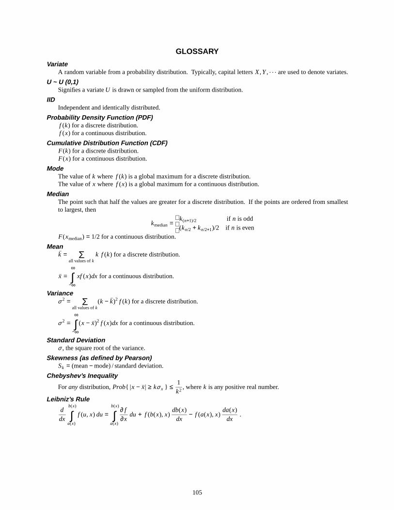
GLOSSARY
VariateA random variable from a probability distribution. Typically, capital letters X,Y, . . . are used to denote variates.
U ~ U (0,1)Signifies a variateU is drawn or sampled from the uniform distribution.
IIDIndependent and identically distributed.
Probability Density Function (PDF)f (k) for a discrete distribution.f (x) for a continuous distribution.
Cumulative Distrib ution Function (CDF)F(k) for a discrete distribution.F(x) for a continuous distribution.
ModeThe value ofk where f (k) is aglobal maximum for a discrete distribution.The value ofx where f (x) is aglobal maximum for a continuous distribution.
MedianThe point such that half the values are greater for a discrete distribution. If the points are ordered from smallestto largest, then
kmedian=
k(n+1)/2
(kn/2 + kn/2+1)/2
if n is odd
if n is evenF(xmedian) = 1/2 for a continuous distribution.
Meank =
all values ofkΣ k f (k) for a discrete distribution.
x =∞
−∞∫ xf (x)dx for a continuous distribution.
Varianceσ 2 =
all values ofkΣ (k − k)2 f (k) for a discrete distribution.
σ 2 =∞
−∞∫ (x − x)2 f (x)dx for a continuous distribution.
Standar d Deviationσ , the square root of the variance.
Skewness (as defined b y Pearson)Sk = (mean− mode) / standard deviation.
Chebyshe v’s Inequality
For anydistribution, Prob{ |x − x| ≥ kσ x } ≤1
k2, wherek is any positive real number.
Leibniz’ s Rule
d
dx
b(x)
a(x)∫ f (u, x) du =
b(x)
a(x)∫ ∂ f
∂xdu + f (b(x), x)
db(x)
dx− f (a(x), x)
da(x)
dx.
105

INTENTIONALLY LEFT BLANK.
106