Probability and statistical distributions for

ecological modeling

©2007 Ben Bolker

August 3, 2007

Summary

This chapter continues to review the math you need to fit models to data, mov-ing forward from functions and curves to probability distributions. The first partdiscusses ecological variability in general terms, then reviews basic probabilitytheory and some important applications, including Bayes’ Rule and its appli-cation in statistics. The second part reviews how to analyze and understandprobability distributions. The third part provides a bestiary of probability dis-tributions, finishing with a short digression on some ways to extend these basicdistributions.

1 Introduction: why does variability matter?

For many ecologists and statisticians, noise is just a nuisance — it gets in theway of drawing conclusions from the data. The traditional statistical approachto noise in data was to assume that all variation in the data was normally dis-tributed, or transform the data until it was, and then use classical methodsbased on the normal distribution to draw conclusions. Some scientists turnedto nonparametric statistics, which assume only that the shape of the data dis-tribution is the same in all categories and provide tests of differences in themeans or “location parameters” among categories. Unfortunately, classical non-parametric approaches make it much harder to draw quantitative conclusionsfrom data (rather than simply rejecting or failing to reject null hypotheses aboutdifferences between groups).

In the 1980s, as they acquired better computing tools, ecologists began touse more sophisticated models of variability such as generalized linear models(see Chapter ??). Chapter ?? illustrated a wide range of deterministic functionsthat correspond to eterministic models of the underlying ecological processes.This chapter will illustrate a wide range of models for the stochastic part of thedynamics. In these models, variability isn’t just a nuisance, but actually tells ussomething about ecological processes. For example, census counts that follow anegative binomial distribution (p. 22) tell us there is some form of environmental

1

variation or aggregative response among individuals that we haven’t taken intoaccount (Shaw and Dobson, 1995).

Remember from Chapter ?? that what we treat as “signal” (deterministic)and what we treat as “noise” (stochastic) depends on the question. The sameecological variability, such as spatial variation in light, might be treated asrandom variation by a forester interested in the net biomass increment of a foreststand and as a deterministic driving factor by an ecophysiologist interested inthe photosynthetic response of individual plants.

Noise affects ecological data in two different ways — as measurement er-ror and as process noise (this will become important in Chapter ?? when wedeal with dynamical models). Measurement error is the variability or “noise” inour measurements, which makes it hard to estimate parameters and make in-ferences about ecological systems. Measurement error leads to large confidenceintervals and low statistical power. Even if we can eliminate measurement error,process noise or process error (often so-called even though it isn’t technicallyan “error”, but a real part of the system) still exists. Variability affects anyecological system. For example, we can observe thousands of individuals to de-termine the average mortality rate with great accuracy. The fate of a group ofa few individuals, however, depends both on the variability in mortality ratesof individuals and on the demographic stochasticity that determines whether aparticular individual lives or dies (“loses the coin toss”). Even though we knowthe average mortality rate perfectly, our predictions are still uncertain. Envi-ronmental stochasticity — spatial and temporal variability in (e.g.) mortalityrate caused by variation in the environment rather than by the inherent ran-domness of individual fates — also affects the dynamics. Finally, even if wecan minimize measurement error by careful measurement and minimize processnoise by studying a large population in a constant environment (i.e. low levelsof demographic and environmental stochasticity), ecological systems can stillamplify variability in surprising ways (Bjørnstad and Grenfell, 2001). For ex-ample, a tiny bit of demographic stochasticity at the beginning of an epidemiccan trigger huge variation in epidemic dynamics (Rand and Wilson, 1991). Vari-ability also feeds back to change the mean behavior of ecological systems. Forexample, in the damselfish system described in Chapter ?? the number of re-cruits in any given cohort is the number of settlers surviving density-dependentmortality, but the average number of recruits is lower than expected from anaverage-sized cohort of settlers because large cohorts suffer disproportionatelyhigh mortality and contribute relatively little to the average. This widespreadphenomenon follows from Jensen’s inequality (Ruel and Ayres, 1999; Inouye,2005).

2 Basic probability theory

In order to understand stochastic terms in ecological models, you’ll have to(re)learn some basic probability theory. To define a probability, we first haveto identify the sample space, the set of all the possible outcomes that could

2

occur. Then the probability of an event A is the frequency with which thatevent occurs. A few probability rules are all you need to know:

1. If two events are mutually exclusive (e.g., ”individual is male” and ”indi-vidual is female”) then the probability that either occurs (the probabilityof A or B, or Prob(A ∪ B)) is the sum of their individual probabilities:e.g. Prob(male or female) = Prob(male) + Prob(female).

We use this rule, for example, in finding the probability that an outcomeis within a certain numeric range by adding up the probabilities of all thedifferent (mutually exclusive) values in the range: for a discrete variable,for example, P (3 ≤ X ≤ 5) = P (X = 3) + P (X = 4) + P (X = 5).

2. If two events A and B are not mutually exclusive — the joint probabilitythat they occur together, Prob(A ∩ B), is greater than zero — then wehave to correct the rule for combining probabilities to account for double-counting:

Prob(A ∪B) = Prob(A) + Prob(B)− Prob(A ∩B).

For example if we are tabulating the color and sex of animals, Prob(blue or male) =Prob(blue) + Prob(male)− Prob(blue male))

3. The probabilities of all possible outcomes of an observation or experimentadd to 1.0. (Prob(male) + Prob(female) = 1.0.)

We will need this rule to understand the form of probability distributions,which often contain a normalization constant to make sure that the sumof the probabilities of all possible outcomes is 1.

4. The conditional probability of A given B, Prob(A|B), is the probabilitythat A happens if we know or assume B happens. The conditional prob-ability equals

Prob(A|B) = Prob(A ∩B)/Prob(B). (1)

For example:

Prob(individual is blue|individual is male) =Prob(individual is a blue male)

Prob(individual is male).

(2)By contrast, we may also refer to the probability of A when we make noassumptions about B as the unconditional probability of A. Prob(A) =Prob(A|B) + Prob(A|not B).

Conditional probability is central to understanding Bayes’ Rule (p. 6).

5. If the conditional probability of A given B, Prob(A|B), equals the uncon-ditional probability of A, then A is independent of B. Knowing about Bprovides no information about the probability of A. Independence impliesthat

Prob(A ∩B) = Prob(A)Prob(B), (3)

3

which follows from multiplying both sides of (1) by Prob(B). The proba-bilities of combinations of independent events are multiplicative.

Multiplying probabilities of independent events, or adding independentlog-probabilities (log(Prob(A ∩ B)) = log(Prob(A)) + log(Prob(B)) if Aand B are independent), is how we find the combined probability of aseries of observations.

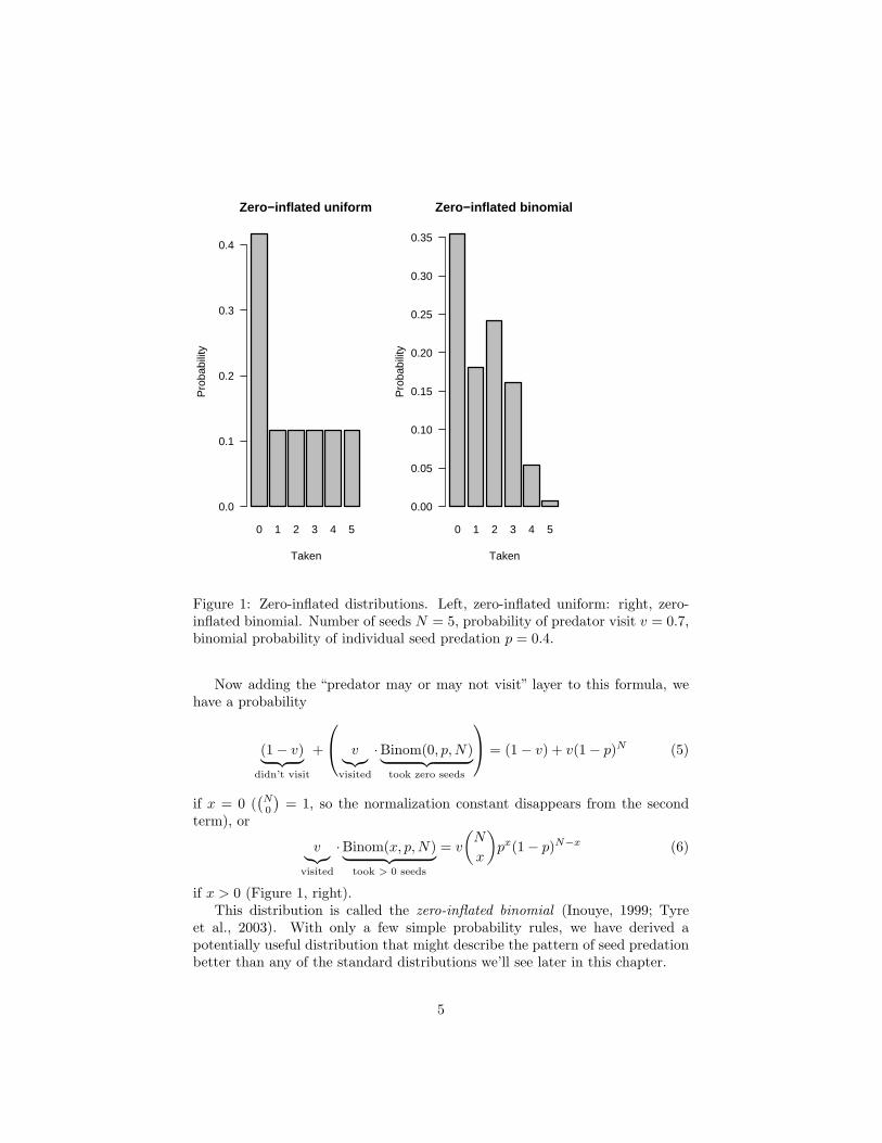
We can immediately use these rules to think about the distribution of seedstaken in the seed removal experiment (Chapter ??). The most obvious patternin the data is that there are many zeros, probably corresponding to times whenno predators visited the station. The sample space for seed disappearance —is the number of seeds taken, from 0 to N (the number available). Supposethat when a predator did visit the station, with probability v, it had an equalprobability of taking any of the possible number of seeds (a uniform distri-bution from 0 to N). Since the probabilities must add to 1, this probability(Prob(x taken|predator visits)) is 1/(N + 1) (0 to N represents N + 1 differentpossible events). What is the unconditional probability of x seeds being taken?

If x > 0, then there is only one possible type of event — the predator visitedand took x seeds — with overall probability v/(N + 1) (Figure 1, left).

If x = 0, then there are two mutually exclusive possibilities. Either thepredator didn’t visit (probability 1 − v), or it visited (probability v) and tookzero seeds (probability 1/(N + 1)), so the overall probability is

(1− v)︸ ︷︷ ︸didn’t visit

+

v︸︷︷︸visited

× 1N + 1︸ ︷︷ ︸

took zero seeds

= 1− v +v

N + 1. (4)

Now make things a little more complicated and suppose that when a predatorvisits, it decides independently whether or not to take each seed. If the seedsof a given species are all identical, so that each seed is taken with the sameprobability p, then this process results in a binomial distribution. Using therules above, the probability of x seeds being taken when each has probability pis px. It’s also true that N −x seeds are not taken, with probability (1−p)N−x.Thus the probability is proportional to px ·(1−p)N−x. To get the probabilities ofall possible outcomes to add to 1, though, we have to multiply by a normalizationconstant N !/(x!(N −x)!)∗, or

(Nx

). (It’s too bad we can’t just ignore these ugly

normalization factors, which are always the least intuitive parts of probabilityformulas, but we really need them in order to get the right answers. Unless youare doing advanced calculations, however, you can usually just take the formulasfor the normalization constants for granted, without trying to puzzle out theirmeaning.)

∗N ! means N · (N − 1) · . . . · 2 · 1, and is referred to as “N factorial”.

4

0 1 2 3 4 5

Zero−inflated uniform

Taken

Pro

babi

lity

0.0

0.1

0.2

0.3

0.4

0 1 2 3 4 5

Zero−inflated binomial

Taken

Pro

babi

lity

0.00

0.05

0.10

0.15

0.20

0.25

0.30

0.35

Figure 1: Zero-inflated distributions. Left, zero-inflated uniform: right, zero-inflated binomial. Number of seeds N = 5, probability of predator visit v = 0.7,binomial probability of individual seed predation p = 0.4.

Now adding the “predator may or may not visit” layer to this formula, wehave a probability

(1− v)︸ ︷︷ ︸didn’t visit

+

v︸︷︷︸visited

·Binom(0, p,N)︸ ︷︷ ︸took zero seeds

= (1− v) + v(1− p)N (5)

if x = 0 ((N0

)= 1, so the normalization constant disappears from the second

term), or

v︸︷︷︸visited

·Binom(x, p, N)︸ ︷︷ ︸took > 0 seeds

= v

(N

x

)px(1− p)N−x (6)

if x > 0 (Figure 1, right).This distribution is called the zero-inflated binomial (Inouye, 1999; Tyre

et al., 2003). With only a few simple probability rules, we have derived apotentially useful distribution that might describe the pattern of seed predationbetter than any of the standard distributions we’ll see later in this chapter.

5

3 Bayes’ Rule

With the simple probability rules defined above we can also derive, and under-stand, Bayes’ Rule. Most of the time we will use Bayes’ Rule to go from thelikelihood Prob(D|H), the probability of observing a particular set of data Dgiven that a hypothesis H is true (p. ??), to the information we really want,Prob(H|D) — the probability of our hypothesis H in light of our data D. Bayes’Rule is just a recipe for turning around a conditional probability:

P (H|D) =P (D|H)P (H)

P (D). (7)

Bayes’ Rule is general — H and D can be any events, not just hypothesisand data — but it’s easier to understand Bayes’ Rule when we have somethingconcrete to tie it to. Deriving Bayes’ Rule is almost as easy as remembering it.Rule #4 on p. 3 applied to P (H|D) implies

P (D ∩H) = P (H|D)P (D), (8)

while applying it to P (D|H) tells us

P (H ∩D) = P (D|H)P (H). (9)

But P (H ∩D) = P (D ∩H) so

P (H|D)P (D) = P (D|H)P (H) (10)

and therefore

P (H|D) =P (D|H)P (H)

P (D). (11)

Equation (11) says that the probability of the hypothesis given (in lightof) the data is equal to the probability of the data given the hypothesis (thelikelihood associated with H), times the probability of the hypothesis, dividedby the probability of the data. There are two problems here: we don’t knowthe probability of the hypothesis, P (H) (isn’t that what we’re trying to figureout in the first place?), and we don’t know the unconditional probability of thedata, P (D).

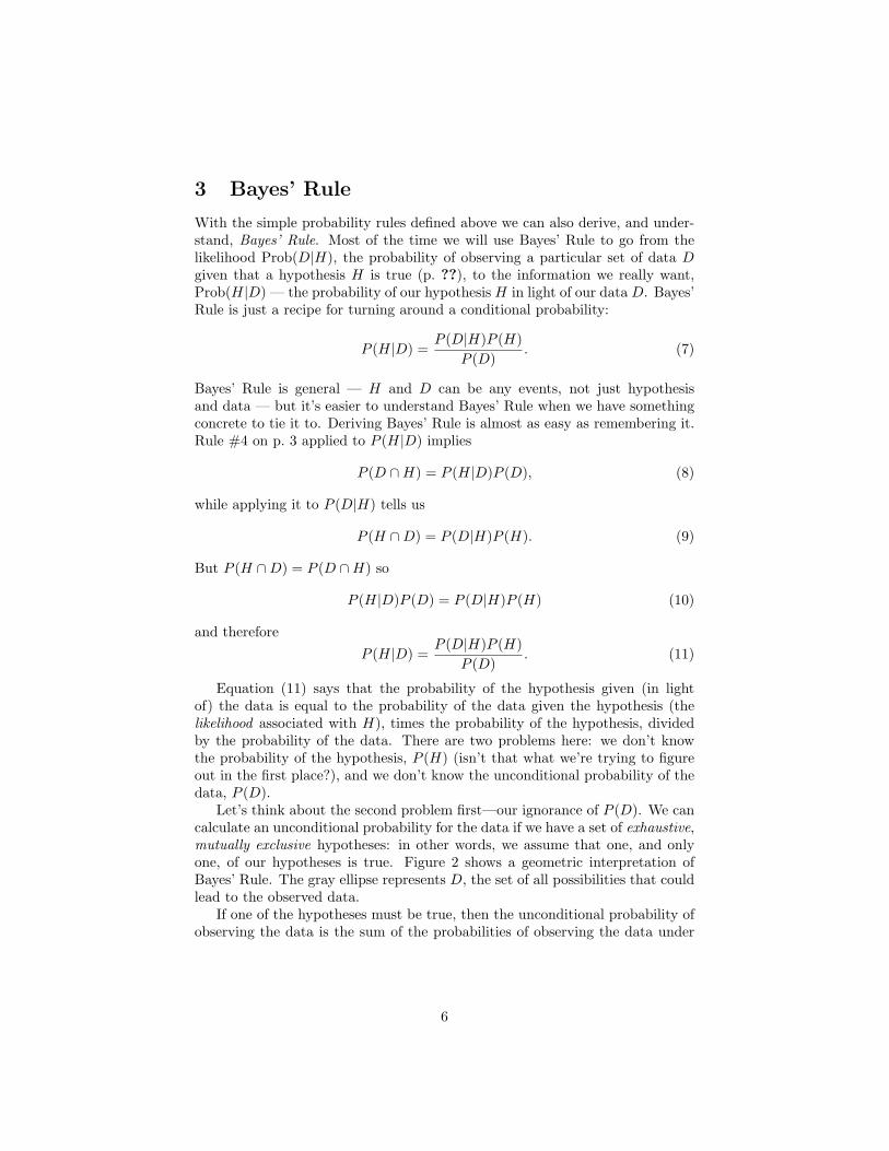
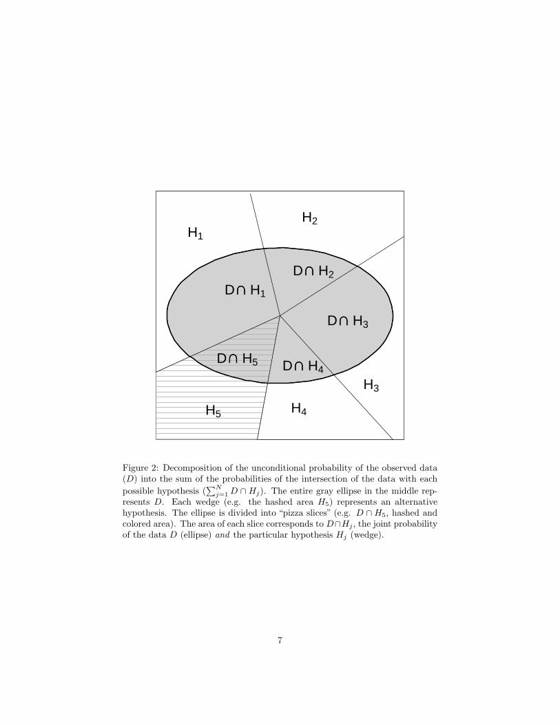
Let’s think about the second problem first—our ignorance of P (D). We cancalculate an unconditional probability for the data if we have a set of exhaustive,mutually exclusive hypotheses: in other words, we assume that one, and onlyone, of our hypotheses is true. Figure 2 shows a geometric interpretation ofBayes’ Rule. The gray ellipse represents D, the set of all possibilities that couldlead to the observed data.

If one of the hypotheses must be true, then the unconditional probability ofobserving the data is the sum of the probabilities of observing the data under

6

H1

D∩∩H1

H2

D∩∩H2

H3

D∩∩H3

H4

D∩∩H4

H5

D∩∩H5

Figure 2: Decomposition of the unconditional probability of the observed data(D) into the sum of the probabilities of the intersection of the data with eachpossible hypothesis (

∑Nj=1 D ∩Hj). The entire gray ellipse in the middle rep-

resents D. Each wedge (e.g. the hashed area H5) represents an alternativehypothesis. The ellipse is divided into “pizza slices” (e.g. D ∩H5, hashed andcolored area). The area of each slice corresponds to D∩Hj , the joint probabilityof the data D (ellipse) and the particular hypothesis Hj (wedge).

7

any of the possible hypotheses, For N different hypotheses H1 to HN ,

P (D) =N∑

j=1

P (D ∩Hj)

=N∑

j=1

P (Hj)P (D|Hj). (12)

In words, the unconditional probability of the data is the sum of the likelihoodof each hypothesis (P (D|Hj)) times its unconditional probability (P (Hj)). InFigure 2, summing the area of overlap of each of the large wedges (the hypothesesHj) with the gray ellipse (Hj ∩D) provides the area of the ellipse (D).

Substituting (12) into (11) gives the full form of Bayes’ Rule for a particularhypothesis Hi when it is one of a mutually exclusive set of hypotheses {Hj}.The probability of the truth of Hi in light of the data is

P (Hi|D) =P (D|Hi)P (Hi)∑j P (Hj)P (D|Hj)

(13)

In Figure 2, having observed the data D means we know that reality liessomewhere in the gray ellipse. The probability that hypothesis 5 is true (i.e.,that we are somewhere in the hashed area) is equal to the area of the hashed/-colored “pizza slice” divided by the area of the ellipse. Bayes’ Rule breaks thisdown further by supposing that we know how to calculate the likelihood of thedata for each hypothesis — the ratio of the pizza slice divided by the area of theentire wedge (the area of the pizza slice [D ∩H5] divided by the hashed wedge[H5]). Then we can recover the area of each slice by multiplying the likelihoodby the prior (the area of the wedge) and calculate both P (D) and P (H5|D).

Dealing with the second problem, our ignorance of the unconditional or priorprobability of the hypothesis P (Hi), is more difficult. In the next section wewill simply assume that we have other information about this probability, andwe’ll revisit the problem shortly in the context of Bayesian statistics. But first,just to practice with Bayes’ Rule, we’ll explore two simpler examples that useBayes’ Rule to manipulate conditional probabilities.

3.1 False positives in medical testing

Suppose the unconditional probability of a random person sampled from thepopulation being infected (I) with some deadly but rare disease is one in a mil-lion: P (I) = 10−6. There is a test for this disease that never gives a false nega-tive result: if you have the disease, you will definitely test positive (P (+|I) = 1).However, the test does occasionally give a false positive result. One person in100 who doesn’t have the disease (is uninfected, U) will test positive anyway(P (+|U) = 10−2). This sounds like a pretty good test. Let’s compute theprobability that someone who tests positive is actually infected.

8

Replace H in Bayes’ rule with “is infected” (I) and D with “tests positive”(+). Then

P (I|+) =P (+|I)P (I)

P (+). (14)

We know P (+|I) = 1 and P (I) = 10−6, but we don’t know P (+), the un-conditional probability of testing positive. Since you are either infected (I) oruninfected (U), so these events are mutually exclusive,

P (+) = P (+ ∩ I) + P (+ ∩ U). (15)

ThenP (+) = P (+|I)P (I) + P (+|U)P (U) (16)

because P (I ∩+) = P (+|I)P (I) (eq. 1). We also know that P (U) = 1− P (I),so

P (+) = P (+|I)P (I) + P (+|U)(1− P (I))

= 1× 10−6 + 10−2 × (1− 10−6)

= 10−6 + 10−2 + 10−8

≈ 10−2.

(17)

Since 10−6 is ten thousand times smaller than 10−2, and 10−8 is even tinier, wecan neglect them for now.

Now that we’ve done the hard work of computing the denominator, we canput it together with the numerator:

P (I|+) =P (+|I)P (I)

P (+)

≈ 1× 10−6

10−2

= 10−4

(18)

Even though false positives are unlikely, the chance that you are infected if youtest positive is still only 1 in 10,000! For a sensitive test (one that producesfew false negatives) for a rare disease, the probability that a positive test isdetecting a true infection is approximately P (I)/P (false positive), which canbe surprisingly small.

This false-positive issue also comes up in forensics cases (DNA testing, etc.).Assuming that a positive test is significant is called the base rate fallacy. It’s im-portant to think carefully about the sample population and the true probabilityof being guilty (or at least having been present at the crime scene) conditionalon having your DNA match DNA found at the crime scene.

3.2 Bayes’ Rule and liana infestation

A student of mine used Bayes’ Rule as part of a simulation model of liana (vine)dynamics in a tropical forest. He wanted to know the probability that a newly

9

emerging sapling would be in a given “liana class” (L1=liana-free, L2–L3=lightto moderate infestation, L4=heavily infested with lianas). This probability de-pends on the number of trees nearby that are already infested (N). We havemeasurements of infestation of saplings from the field, and for each one weknow the number of nearby infestations. Thus if we calculate the fraction ofindividuals in liana class Li with N nearby infested trees, we get an estimate ofProb(N |Li). We also know the overall fractions in each liana class, Prob(Li).When we add a new tree to the model, we know the neighborhood infestationN from the model. Thus we can figure out what we want to know, Prob(Li|N),by using Bayes’ Rule to calculate

Prob(Li|N) =Prob(N |Li)Prob(Li)∑4

j=1 Prob(N |Lj)Prob(Lj). (19)

For example, suppose we find that a new tree in the model has 3 infested neigh-bors. Let’s say that the probabilities of each liana class (1 to 4) having 3infested neighbors are Prob(N |Li) = {0.05, 0.1, 0.3, 0.6} and that the uncondi-tional probabilities of being in each liana class are Li = {0.5, 0.25, 0.2, 0.05}.Then the probability that the new tree is heavily infested (i.e. is in class L4) is

0.6× 0.05(0.05× 0.5) + (0.1× 0.25) + (0.3× 0.2) + (0.6× 0.05)

= 0.21. (20)

We would expect that a new tree with several infested neighbors has a muchhigher probability of heavy infestation than the overall (unconditional) proba-bility of 0.05. Bayes’ Rule allows us to quantify this guess.

3.3 Bayes’ Rule in Bayesian statistics

So what does Bayes’ Rule have to do with Bayesian statistics?Bayesians translate likelihood into information about parameter values us-

ing Bayes’ Rule as given above. The problem is that we have the likelihoodL(data|hypothesis), the probability of observing the data given the model (pa-rameters): what we want is Prob(hypothesis|data). After all, we already knowwhat the data are!

3.3.1 Priors

In the disease testing and the liana examples, we knew the overall, uncondi-tional probability of disease or liana class in the population. When we’re doingBayesian statistics, however, we interpret P (Hi) instead as the prior probabil-ity of a hypothesis, our belief about the probability of a particular hypothesisbefore we see the data. Bayes’ Rule is the formula for updating the prior inorder to compute the posterior probability of each hypothesis, our belief aboutthe probability of the hypothesis after we see the data. Suppose I have twohypotheses A and B and have observed some data D with likelihoods LA = 0.1and LB = 0.2. In other words, the probability of D occurring if hypothesis A is

10

true (P (D|A)) is 10%, while the probability of D occurring if hypothesis B istrue (P (D|B)) is 20%. If I assign the two hypotheses equal prior probabilities(0.5 each), then Bayes’ Rule says the posterior probability of A is

P (A|D) =0.1× 0.5

0.1× 0.5 + 0.2× 0.5=

0.10.3

=13

(21)

and the posterior probability of B is 2/3. However, if I had prior informationthat said A was twice as probable (Prob(A) = 2/3, Prob(B) = 1/3) then theprobability of A given the data would be 0.5 (do the calculation). It is inprinciple possible to get whatever answer you want, by rigging the prior: if youassign B a prior probability of 0, then no data will ever convince you that Bis true (in which case you probably shouldn’t have done the experiment in thefirst place). Frequentists claim that this possibility makes Bayesian statisticsopen to cheating (Dennis, 1996): however, every Bayesian analysis must clearlystate the prior probabilities it uses. If you have good reason to believe that theprior probabilities are not equal, from previous studies of the same or similarsystems, then arguably you should use that information rather than startingas frequentists do from the ground up every time. (The frequentist-Bayesiandebate is one of the oldest and most virulent controversies in statistics (Ellison,1996; Dennis, 1996): I can’t possibly do it justice here.)

However, it is a good idea to try so-called flat or weak or uninformativepriors — priors that assume you have little information about which hypothesisis true — as a part of your analysis, even if you do have prior information(Edwards, 1996). You may have noticed in the first example above that whenwe set the prior probabilities equal, the posterior probabilities were just equalto the likelihoods divided by the sum of the likelihoods. Algebraically if all theP (Hi) are equal to the same constant C,

P (Hi|D) =P (D|Hi)C∑j P (D|Hj)C

=Li∑j Lj

(22)

where Li is the likelihood of hypothesis i.You may think that setting all the priors equal would be an easy way to elim-

inate the subjective nature of Bayesian statistics and make everybody happy.Two examples, however, will demonstrate that it’s not that easy to say what itmeans to be completely “objective” or ignorant of the right hypothesis.

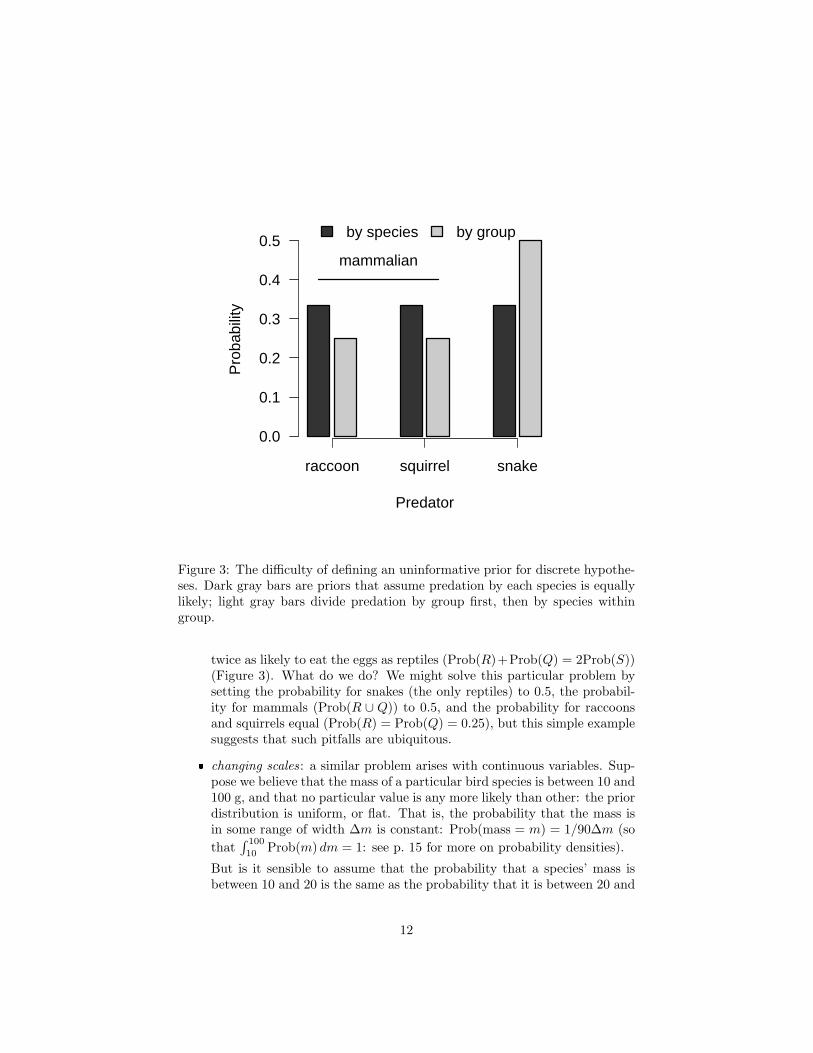
� partitioning hypotheses: suppose we find a nest missing eggs that mighthave been taken by a raccoon, a squirrel, or a snake (only). The threehypotheses “raccoon” (R), “squirrel” (Q), and “snake” (S) are our mu-tually exclusive and exhaustive set of hypotheses for the identity of thepredator. If we have no other information (for example about the localdensities or activity levels of different predators), we might choose equalprior probabilities for all three hypotheses. Since there are three mutuallyexclusive predators, Prob(R) = Prob(Q) = Prob(S) = 1/3. Now a friendcomes and asks us whether we really believe that mammalian predators are

11

Predator

Pro

babi

lity

0.0

0.1

0.2

0.3

0.4

0.5

raccoon squirrel snake

mammalian

by species by group

Figure 3: The difficulty of defining an uninformative prior for discrete hypothe-ses. Dark gray bars are priors that assume predation by each species is equallylikely; light gray bars divide predation by group first, then by species withingroup.

twice as likely to eat the eggs as reptiles (Prob(R)+Prob(Q) = 2Prob(S))(Figure 3). What do we do? We might solve this particular problem bysetting the probability for snakes (the only reptiles) to 0.5, the probabil-ity for mammals (Prob(R ∪ Q)) to 0.5, and the probability for raccoonsand squirrels equal (Prob(R) = Prob(Q) = 0.25), but this simple examplesuggests that such pitfalls are ubiquitous.

� changing scales: a similar problem arises with continuous variables. Sup-pose we believe that the mass of a particular bird species is between 10 and100 g, and that no particular value is any more likely than other: the priordistribution is uniform, or flat. That is, the probability that the mass isin some range of width ∆m is constant: Prob(mass = m) = 1/90∆m (sothat

∫ 100

10Prob(m) dm = 1: see p. 15 for more on probability densities).

But is it sensible to assume that the probability that a species’ mass isbetween 10 and 20 is the same as the probability that it is between 20 and

12

linear scale

Mass

Pro

babi

lity

dens

ity

10 100

0.00

0.02

0.04uniformlog−uniform

log scale

Log mass

log(10) log(100)

0.0

0.5

1.0

Figure 4: The difficulty of defining an uninformative prior on continuous scales.If we assume that the probabilities are uniform on one scale (linear or logarith-mic), they must be non-uniform on the other.

30, or should it be the same as the probability that it is between 20 and 40— that is, would it make more sense to think of the mass distribution ona logarithmic scale? If we say that the probability distribution is uniformon a logarithmic scale, then a species is less likely to be between 20 and30 than it is to be between 10 and 20.∗ Since changing the scale is notreally changing anything about the world, just the way we describe it, thischange in the prior is another indication that it’s harder than we thinkto say what it means to be ignorant. In any case, many Bayesians thinkthat researchers try too hard to pretend ignorance, and that one reallyshould use what is known about the system. Crome et al. (1996) compareextremely different priors in a conservation context to show that their datareally are (or should be) informative to a wide spectrum of stakeholders,regardless of their perspectives.

3.3.2 Integrating the denominator

The other challenge with Bayesian statistics, which is purely technical and doesnot raise any deep conceptual issues, is the problem of adding up the denomi-

∗If the probability is uniform between a and b on the usual, linear scale (Prob(mass =m) = 1/(b− a) dm), then on the log scale it is Prob(log mass = M) = 1/(b− a)eM dM [if wechange variables to log mass M , then dM = d(log m) = 1/m dm, so dm = m dM = eM dM ].Going the other way, a log-uniform assumption gives Prob(mass = m) = 1/(log(b/a)m)dmon the linear scale.

13

nator∑

j P (Hj)P (D|Hj) in Bayes’ rule. If the set of hypotheses (parameters)is continuous, then the denominator is

∫P (h)P (D|h) dh where h is a particular

parameter value.For example, the binomial distribution says that the likelihood of obtaining 2

heads in 3 (independent, equal-probability) coin flips is(32

)p2(1− p), a function

of p. The likelihood for p = 0.5 is therefore 0.375, but to get the posteriorprobability we have to divide by the probability of getting 2 heads in 3 flips forany value of p. Assuming a flat prior, the denominator is

∫ 1

0

(32

)p2(1 − p) dp =

0.25, so the posterior probability density of p = 0.5 is 0.375/0.25 = 1.5∗.For the binomial case and other simple probability distributions, it’s easy

to sum or integrate the denominator either analytically or numerically. If weonly care about the relative probability of different hypotheses, we don’t needto integrate the denominator because it has the same constant value for everyhypothesis.

Often, however, we do want to know the absolute probability. Calculatingthe unconditional probability of the data (the denominator for Bayes’ Rule) canbe extremely difficult for more complicated problems. Much of current researchin Bayesian statistics focuses on ways to calculate the denominator. We willrevisit this problem in Chapters ?? and ??, first integrating the denominatorby brute-force numerical integration, then looking briefly at a sophisticatedtechnique for Bayesian analysis called Markov chain Monte Carlo.

3.4 Conjugate priors

Using so-called conjugate priors makes it easy to do the math for Bayesian analy-sis. Imagine that we’re flipping coins (or measuring tadpole survival or countingnumbers of different morphs in a fixed sample) and that we use the binomialdistribution to model the data. For a binomial with a per-trial probability ofp and N trials, the probability of x successes is proportional (leaving out thenormalization constant) to px(1 − p)N−x. Suppose that instead of describingthe probability of x successes with a fixed per-trial probability p and number oftrials N we wanted to describe the probability of a given per-trial probabilityp with fixed x and N . We would get Prob(p) proportional to px(1 − p)N−x

— exactly the same formula, but with a different proportionality constant anda different interpretation. Instead of a discrete probability distribution over asample space of all possible numbers of successes (0 to N), now we have a contin-uous probability distribution over all possible probabilities (all values between0 and 1). The second distribution, for Prob(p), is called the Beta distribution(p. 34) and it is the conjugate prior for the binomial distribution.

Mathematically, conjugate priors have the same structure as the probabilitydistribution of the data. They lead to a posterior distribution with the samemathematical form as the prior, although with different parameter values. Intu-itively, you get a conjugate prior by turning the likelihood around to ask about

∗This value is a probability density, not a probability, so it’s OK for it to be greater than1: probability density will be explained on p. 15.

14

the probability of a parameter instead of the probability of the data.We’ll come back to conjugate priors and how to use them in Chapters ??

and ??.

4 Analyzing probability distributions

You need the same kinds of skills and intuitions about the characteristics ofprobability distributions that we developed in Chapter ?? for mathematicalfunctions.

4.1 Definitions

Discrete A probability distribution is the set of probabilities on a samplespace or set of outcomes. Since this book is about modeling quantitative data,we will always be dealing with sample spaces that are numbers — the numberor amount observed in some measurement of an ecological system. The simplestdistributions to understand are discrete distributions whose outcomes are a setof integers: most of the discrete distributions we’ll deal with describe counting orsampling processes and have ranges that include some or all of the non-negativeintegers.

A discrete distribution is most easily described by its distribution function,which is just a formula for the probability that the outcome of an experimentor observation (called a random variable) X is equal to a particular value x(f(x) = Prob(X = x)). A distribution can also be described by its cumulativedistribution function F (x) (note the uppercase F ), which is the probability thatthe random variable X is less than or equal to a particular value x (F (x) =Prob(X ≤ x). Cumulative distribution functions are most useful for frequentistcalculations of tail probabilities, e.g. the probability of getting n or more headsin a series of coin-tossing experiments with a given trial probability.

Continuous A probability distribution over a continuous range (such as allreal numbers, or the non-negative real numbers) is called a continuous dis-tribution. The cumulative distribution function of a continuous distribution(F (x) = Prob(X ≤ x) is easy to define and understand — it’s just the probabil-ity that the continuous random variable X is smaller than a particular value xin any given observation or experiment — but the probability density function(the analogue of the distribution function for a discrete distribution) is moreconfusing, since the probability of any precise value is zero. You may imaginethat a measurement of (say) pH is exactly 7.9, but in fact what you have ob-served is that the pH is between 7.82 and 7.98 — if your meter has a precisionof ± 1%. Thus continuous probability distributions are expressed as probabilitydensities rather than probabilities — the probability that random variable Xis between x and x + ∆x, divided by ∆x (Prob(7.82 < X < 7.98)/0.16, in thiscase). Dividing by ∆x allows the observed probability density to have a well-defined limit as precision increases and ∆x shrinks to zero. Unlike probabilities,

15

Pro

babi

lity

0 1 2 3 4 5

0.0

0.4

Cum

ulat

ive

prob

abili

ty

0 1 2 3 4 5

0

1

x

Pro

babi

lity

dens

ity

0 6

0.0

1.5

x

Cum

ulat

ive

prob

abili

ty

0 6

0

1

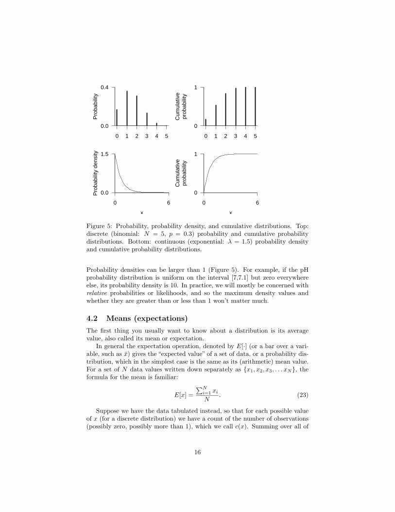
Figure 5: Probability, probability density, and cumulative distributions. Top:discrete (binomial: N = 5, p = 0.3) probability and cumulative probabilitydistributions. Bottom: continuous (exponential: λ = 1.5) probability densityand cumulative probability distributions.

Probability densities can be larger than 1 (Figure 5). For example, if the pHprobability distribution is uniform on the interval [7,7.1] but zero everywhereelse, its probability density is 10. In practice, we will mostly be concerned withrelative probabilities or likelihoods, and so the maximum density values andwhether they are greater than or less than 1 won’t matter much.

4.2 Means (expectations)

The first thing you usually want to know about a distribution is its averagevalue, also called its mean or expectation.

In general the expectation operation, denoted by E[·] (or a bar over a vari-able, such as x̄) gives the “expected value” of a set of data, or a probability dis-tribution, which in the simplest case is the same as its (arithmetic) mean value.For a set of N data values written down separately as {x1, x2, x3, . . . xN}, theformula for the mean is familiar:

E[x] =∑N

i=1 xi

N. (23)

Suppose we have the data tabulated instead, so that for each possible valueof x (for a discrete distribution) we have a count of the number of observations(possibly zero, possibly more than 1), which we call c(x). Summing over all of

16

the possible values of x, we have

E[x] =∑N

i=1 xi

N=

∑c(x)xN

=∑ (

c(x)N

)x =

∑Prob(x)x (24)

where Prob(x) is the discrete probability distribution representing this partic-ular data set. More generally, you can think of Prob(x) as representing someparticular theoretical probability distribution which only approximately matchesany actual data set.

We can compute the mean of a continuous distribution as well. First, let’sthink about grouping (or “binning”) the values in a discrete distribution intocategories of size ∆x. Then if p(x), the density of counts in bin x, is c(x)/∆x, theformula for the mean becomes

∑p(x)·x∆x. If we have a continuous distribution

with ∆x very small, this becomes∫

p(x)x dx. (This is in fact the definition ofan integral.) For example, an exponential distribution p(x) = λ exp(−λx) hasan expectation or mean value of

∫λ exp(−λx)x dx = 1/λ. (You don’t need to

know how to do this integral analytically, although the R supplement will showa little bit about numerical integration in R.)

4.3 Variances (expectation of X2)

The mean is the expectation of the random variable X itself, but we can alsoask about the expectation of functions of X. The first example is the expec-tation of X2. We just fill in the value x2 for x in all of the formulas above:E[x2] =

∑Prob(x)x2 for a discrete distribution, or

∫p(x)x2 dx for a continu-

ous distribution. (We are not asking for∑

Prob(x2)x2.) The expectation ofx2 is a component of the variance, which is the expected value of (x − E[x])2

or (x− x̄)2, or the expected squared deviation around the mean. (We can alsoshow that

E[(x− x̄)2] = E[x2]− (x̄)2 (25)

by using the rules for expectations that (1) E[x + y] = E[x] + E[y] and (2) ifc is a constant, E[cx] = cE[x]. The right-hand formula formula is simpler tocompute than E[(x− x̄)2], but more subject to roundoff error.)

Variances are easy to work with because they are additive (we will show laterthat Var(a + b) = Var(a) + Var(b) if a and b are uncorrelated), but harder tocompare with means since their units are the units of the mean squared. Thuswe often use instead the standard deviation of a distribution, (

√Var), which has

the same units as X.Two other summaries related to the variance are the variance-to-mean ratio

and the coefficient of variation (CV), which is the ratio of the standard deviationto the mean. The variance-to-mean ratio has units equal to the mean; it isprimarily used to characterize discrete sampling distributions and compare themto the Poisson distribution, which has a variance-to-mean ratio of 1. The CVis more common, and is useful when you want to describe variation that isproportional to the mean. For example, if you have a pH meter that is accurate

17

to±10%, so that a true pH value of x will give measured values that are normallydistributed with 2σ = 0.1x∗, then σ = 0.05x and the CV is 0.05.

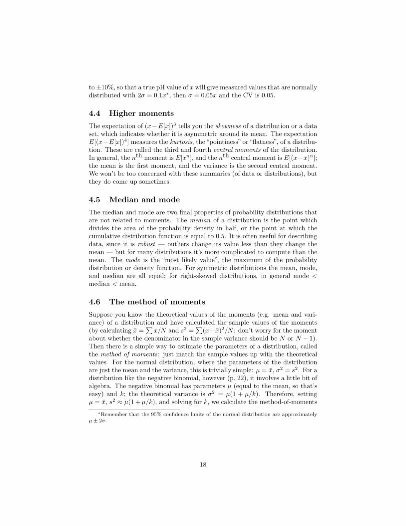
4.4 Higher moments

The expectation of (x−E[x])3 tells you the skewness of a distribution or a dataset, which indicates whether it is asymmetric around its mean. The expectationE[(x−E[x])4] measures the kurtosis, the “pointiness” or “flatness”, of a distribu-tion. These are called the third and fourth central moments of the distribution.In general, the nth moment is E[xn], and the nth central moment is E[(x− x̄)n];the mean is the first moment, and the variance is the second central moment.We won’t be too concerned with these summaries (of data or distributions), butthey do come up sometimes.

4.5 Median and mode

The median and mode are two final properties of probability distributions thatare not related to moments. The median of a distribution is the point whichdivides the area of the probability density in half, or the point at which thecumulative distribution function is equal to 0.5. It is often useful for describingdata, since it is robust — outliers change its value less than they change themean — but for many distributions it’s more complicated to compute than themean. The mode is the “most likely value”, the maximum of the probabilitydistribution or density function. For symmetric distributions the mean, mode,and median are all equal; for right-skewed distributions, in general mode <median < mean.

4.6 The method of moments

Suppose you know the theoretical values of the moments (e.g. mean and vari-ance) of a distribution and have calculated the sample values of the moments(by calculating x̄ =

∑x/N and s2 =

∑(x−x̄)2/N : don’t worry for the moment

about whether the denominator in the sample variance should be N or N − 1).Then there is a simple way to estimate the parameters of a distribution, calledthe method of moments: just match the sample values up with the theoreticalvalues. For the normal distribution, where the parameters of the distributionare just the mean and the variance, this is trivially simple: µ = x̄, σ2 = s2. For adistribution like the negative binomial, however (p. 22), it involves a little bit ofalgebra. The negative binomial has parameters µ (equal to the mean, so that’seasy) and k; the theoretical variance is σ2 = µ(1 + µ/k). Therefore, settingµ = x̄, s2 ≈ µ(1 + µ/k), and solving for k, we calculate the method-of-moments

∗Remember that the 95% confidence limits of the normal distribution are approximatelyµ± 2σ.

18

estimate of k:

σ2 = µ(1 + µ/k)

s2 ≈ x̄(1 + x̄/k)

s2

x̄− 1 ≈ x̄

k

k ≈ x̄

s2/x̄− 1

(26)

The method of moments is very simple but is biased in many cases; it’sa good way to get a first estimate of the parameters of a distribution, butfor serious work you should follow it up with a maximum likelihood estimator(Chapter ??).

5 Bestiary of distributions

The rest of the chapter presents brief introductions to a variety of useful prob-ability distributions, including the mechanisms behind them and some of theirbasic properties. Like the bestiary in Chapter ??, you can skim this bestiaryon the first reading. The appendix of Gelman et al. (1996) contains a usefultable, more abbreviated than these descriptions but covering a wider range offunctions. The book by Evans et al. (2000) is also useful.

5.1 Discrete models

5.1.1 Binomial

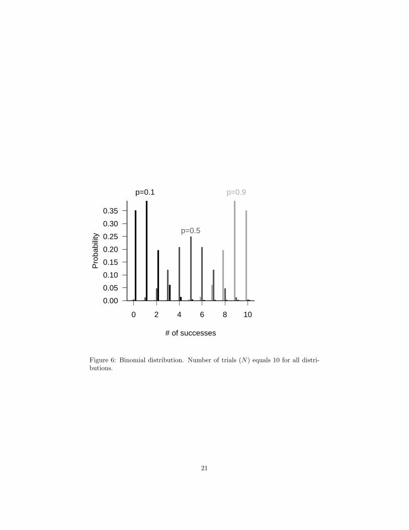
The binomial is probably the easiest distribution to understand. It applies whenyou have samples with a fixed number of subsamples or “trials” in each one,and each trial can have one of two values (black/white, heads/tails, alive/dead,species A/species B), and the probability of“success”(black, heads, alive, speciesA) is the same in every trial. If you flip a coin 10 times (N = 10) and theprobability of a head in each coin flip is p = 0.7 then the probability of getting 7heads (k = 7) will will have a binomial distribution with parameters N = 10 andp = 0.7∗ Don’t confuse the trials (subsamples), and the probability of successin each trial, with the number of samples and the probabilities of the numberof successful trials in each sample. In the seed predation example, a trial is anindividual seed and the trial probability is the probability that an individual seedis taken, while a sample is the observation of a particular station at a particulartime and the binomial probabilities are the probabilities that a certain totalnumber of seeds disappears from the station. You can derive the part of the

∗Gelman and Nolan (2002) point out that it is not physically possible to construct a cointhat is biased when flipped — although a spinning coin can be biased. Diaconis et al. (2004)even tested a coin made of balsa wood on one side and lead on the other to establish that itwas unbiased.

19

distribution that depends on x, px(1−p)N−x, by multiplying the probabilities ofx independent successes with probability p and N −x independent failures withprobability 1− p. The rest of the distribution function,

(Nx

)= N !/(x!(N − x)!),

is a normalization constant that we can justify either with a combinatorialargument about the number of different ways of sampling x objects out of aset of N (Appendix), or simply by saying that we need a factor in front of theformula to make sure the probabilities add up to 1.

The variance of the binomial is Np(1 − p). Like most discrete samplingdistributions (e.g. the binomial, Poisson, negative binomial), this variance de-pends on the number of samples per trial N . When the number of samplesper trial increases the variance also increases, but the coefficient of variation(√

Np(1− p)/(Np) =√

(1− p)/(Np)) decreases. The dependence on p(1 − p)means the binomial variance is small when p is close to 0 or 1 (and therefore thevalues are scrunched up near 0 or N), and largest when p = 0.5. The coefficientof variation, on the other hand, is largest for small p.

When N is large and p isn’t too close to 0 or 1 (i.e. when Np is large), thenthe binomial distribution is approximately normal (Figure 17).

A binomial distribution with only one trial (N = 1) is called a Bernoullitrial.

You should only use the binomial in fitting data when there is an upper limitto the number of possible successes. When N is large and p is small, so that theprobability of getting N successes is small, the binomial approaches the Poissondistribution, which is covered in the next section (Figure 17).

Examples: number of surviving individuals/nests out of an initial sample;number of infested/infected animals, fruits, etc. in a sample; number of a par-ticular class (haplotype, subspecies, etc.) in a larger population.

Summary:range discrete, 0 ≤ x ≤ N

distribution(Nx

)px(1− p)N−x

R dbinom, pbinom, qbinom, rbinomparameters p [real, 0–1], probability of success [prob]

N [positive integer], number of trials [size]mean Npvariance Np(1− p)CV

√(1− p)/(Np)

Conjugate prior Beta

5.1.2 Poisson

The Poisson distribution gives the distribution of the number of individuals,arrivals, events, counts, etc., in a given time/space/unit of counting effort ifeach event is independent of all the others. The most common definition of thePoisson has only one parameter, the average density or arrival rate, λ, whichequals the expected number of counts in a sampling unit. An alternative pa-rameterization gives a density per unit sampling effort and then specifies themean as the product of the density per sampling effort r times the sampling

20

0 2 4 6 8 10

0.00

0.05

0.10

0.15

0.20

0.25

0.30

0.35

# of successes

Pro

babi

lity

p=0.1

p=0.5

p=0.9

Figure 6: Binomial distribution. Number of trials (N) equals 10 for all distri-butions.

21

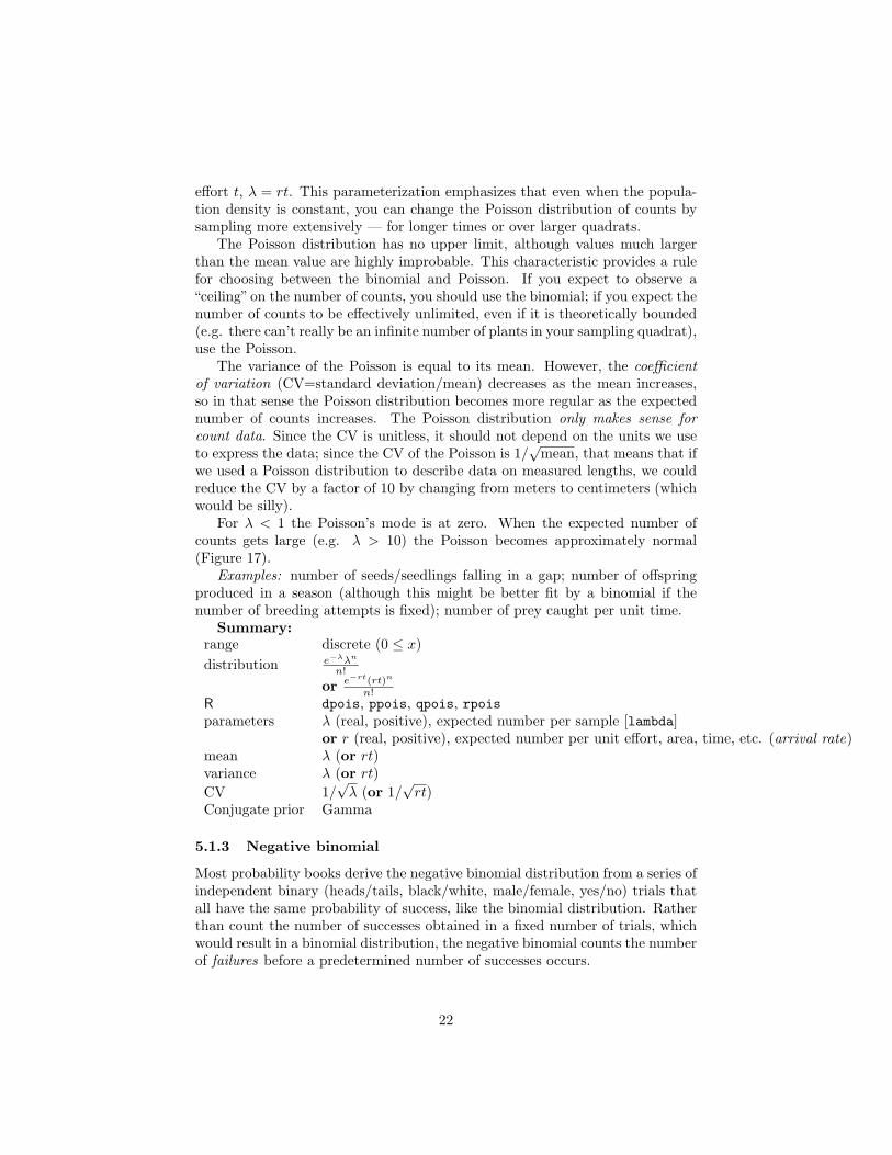
effort t, λ = rt. This parameterization emphasizes that even when the popula-tion density is constant, you can change the Poisson distribution of counts bysampling more extensively — for longer times or over larger quadrats.

The Poisson distribution has no upper limit, although values much largerthan the mean value are highly improbable. This characteristic provides a rulefor choosing between the binomial and Poisson. If you expect to observe a“ceiling”on the number of counts, you should use the binomial; if you expect thenumber of counts to be effectively unlimited, even if it is theoretically bounded(e.g. there can’t really be an infinite number of plants in your sampling quadrat),use the Poisson.

The variance of the Poisson is equal to its mean. However, the coefficientof variation (CV=standard deviation/mean) decreases as the mean increases,so in that sense the Poisson distribution becomes more regular as the expectednumber of counts increases. The Poisson distribution only makes sense forcount data. Since the CV is unitless, it should not depend on the units we useto express the data; since the CV of the Poisson is 1/

√mean, that means that if

we used a Poisson distribution to describe data on measured lengths, we couldreduce the CV by a factor of 10 by changing from meters to centimeters (whichwould be silly).

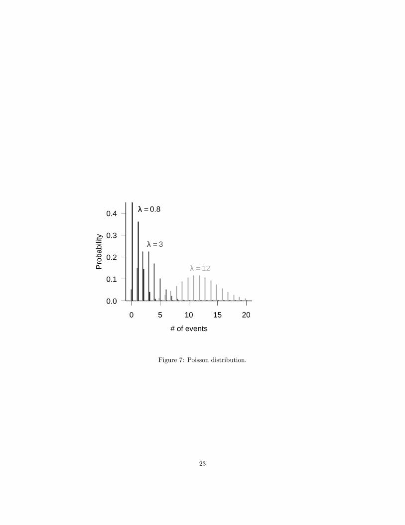
For λ < 1 the Poisson’s mode is at zero. When the expected number ofcounts gets large (e.g. λ > 10) the Poisson becomes approximately normal(Figure 17).

Examples: number of seeds/seedlings falling in a gap; number of offspringproduced in a season (although this might be better fit by a binomial if thenumber of breeding attempts is fixed); number of prey caught per unit time.

Summary:range discrete (0 ≤ x)distribution e−λλn

n!

or e−rt(rt)n

n!R dpois, ppois, qpois, rpoisparameters λ (real, positive), expected number per sample [lambda]

or r (real, positive), expected number per unit effort, area, time, etc. (arrival rate)mean λ (or rt)variance λ (or rt)CV 1/

√λ (or 1/

√rt)

Conjugate prior Gamma

5.1.3 Negative binomial

Most probability books derive the negative binomial distribution from a series ofindependent binary (heads/tails, black/white, male/female, yes/no) trials thatall have the same probability of success, like the binomial distribution. Ratherthan count the number of successes obtained in a fixed number of trials, whichwould result in a binomial distribution, the negative binomial counts the numberof failures before a predetermined number of successes occurs.

22

0 5 10 15 20

0.0

0.1

0.2

0.3

0.4

# of events

Pro

babi

lity

λλ == 0.8

λλ == 3

λλ == 12

Figure 7: Poisson distribution.

23

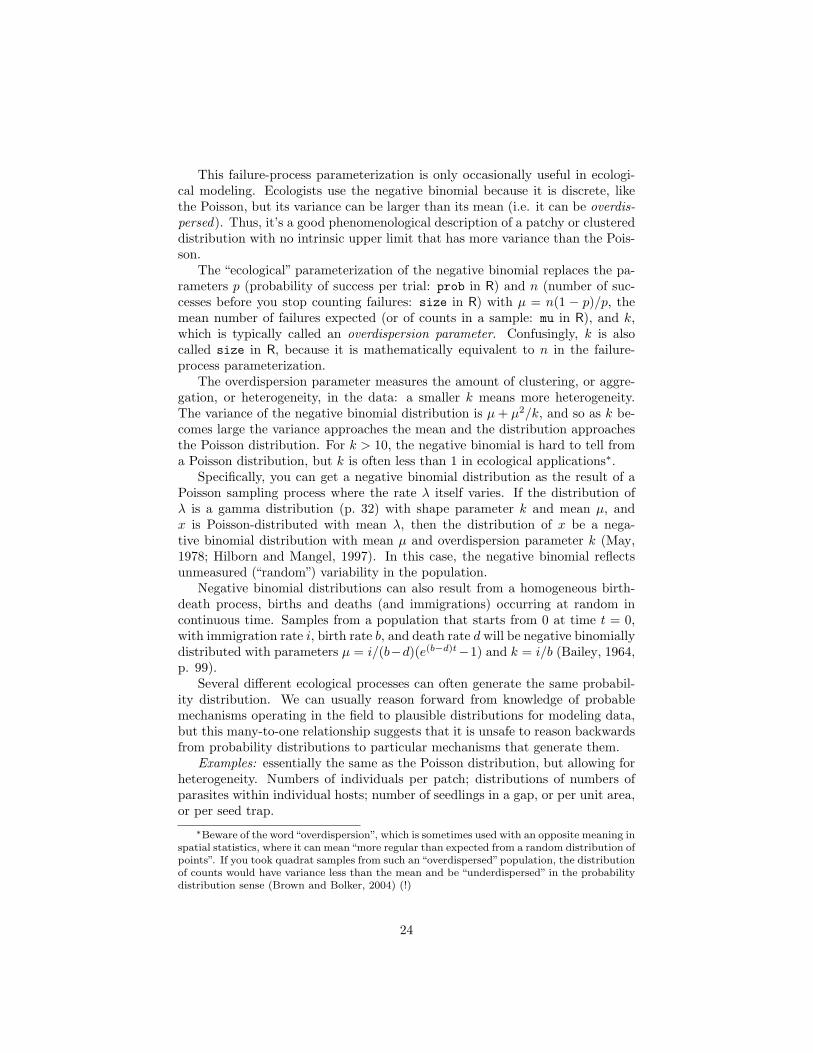
This failure-process parameterization is only occasionally useful in ecologi-cal modeling. Ecologists use the negative binomial because it is discrete, likethe Poisson, but its variance can be larger than its mean (i.e. it can be overdis-persed). Thus, it’s a good phenomenological description of a patchy or clustereddistribution with no intrinsic upper limit that has more variance than the Pois-son.

The “ecological” parameterization of the negative binomial replaces the pa-rameters p (probability of success per trial: prob in R) and n (number of suc-cesses before you stop counting failures: size in R) with µ = n(1 − p)/p, themean number of failures expected (or of counts in a sample: mu in R), and k,which is typically called an overdispersion parameter. Confusingly, k is alsocalled size in R, because it is mathematically equivalent to n in the failure-process parameterization.

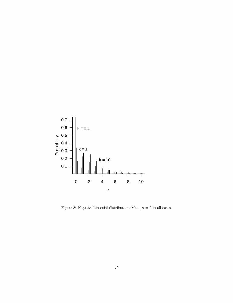
The overdispersion parameter measures the amount of clustering, or aggre-gation, or heterogeneity, in the data: a smaller k means more heterogeneity.The variance of the negative binomial distribution is µ + µ2/k, and so as k be-comes large the variance approaches the mean and the distribution approachesthe Poisson distribution. For k > 10, the negative binomial is hard to tell froma Poisson distribution, but k is often less than 1 in ecological applications∗.

Specifically, you can get a negative binomial distribution as the result of aPoisson sampling process where the rate λ itself varies. If the distribution ofλ is a gamma distribution (p. 32) with shape parameter k and mean µ, andx is Poisson-distributed with mean λ, then the distribution of x be a nega-tive binomial distribution with mean µ and overdispersion parameter k (May,1978; Hilborn and Mangel, 1997). In this case, the negative binomial reflectsunmeasured (“random”) variability in the population.

Negative binomial distributions can also result from a homogeneous birth-death process, births and deaths (and immigrations) occurring at random incontinuous time. Samples from a population that starts from 0 at time t = 0,with immigration rate i, birth rate b, and death rate d will be negative binomiallydistributed with parameters µ = i/(b−d)(e(b−d)t−1) and k = i/b (Bailey, 1964,p. 99).

Several different ecological processes can often generate the same probabil-ity distribution. We can usually reason forward from knowledge of probablemechanisms operating in the field to plausible distributions for modeling data,but this many-to-one relationship suggests that it is unsafe to reason backwardsfrom probability distributions to particular mechanisms that generate them.

Examples: essentially the same as the Poisson distribution, but allowing forheterogeneity. Numbers of individuals per patch; distributions of numbers ofparasites within individual hosts; number of seedlings in a gap, or per unit area,or per seed trap.

∗Beware of the word“overdispersion”, which is sometimes used with an opposite meaning inspatial statistics, where it can mean“more regular than expected from a random distribution ofpoints”. If you took quadrat samples from such an“overdispersed”population, the distributionof counts would have variance less than the mean and be “underdispersed” in the probabilitydistribution sense (Brown and Bolker, 2004) (!)

24

0 2 4 6 8 10

0.1

0.2

0.3

0.4

0.5

0.6

0.7

x

Pro

babi

lity

k == 10

k == 1

k == 0.1

Figure 8: Negative binomial distribution. Mean µ = 2 in all cases.

25

Summary:range discrete, x ≥ 0distribution (n+x−1)!

(n−1!)x! pn(1− p)x

or Γ(k+x)Γ(k)x! (k/(k + µ))k(µ/(k + µ))x

R dnbinom, pnbinom, qnbinom, rnbinomparameters p (0 < p < 1) probability per trial [prob]

or µ (real, positive) expected number of counts [mu]n (positive integer) number of successes awaited [size]or k (real, positive), overdispersion parameter [size]

(= shape parameter of underlying heterogeneity)mean µ = n(1− p)/pvariance µ + µ2/k = n(1− p)/p2

CV√

(1+µ/k)µ = 1/

√n(1− p)

Conjugate prior No simple conjugate prior (Bradlow et al., 2002)R’s default coin-flipping (n =size, p =prob) parameterization. In order to

use the “ecological” (µ =mu, k =size) parameterization, you must name the muparameter explicitly (e.g. dnbinom(5,size=0.6,mu=1)).

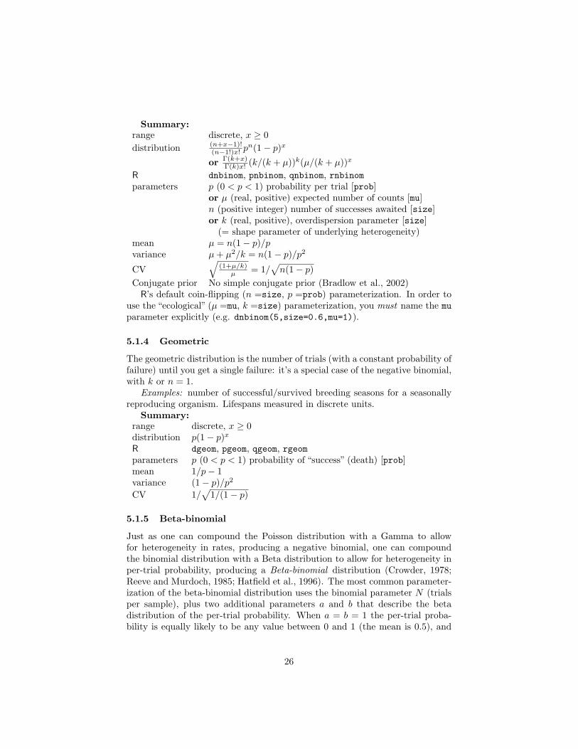
5.1.4 Geometric

The geometric distribution is the number of trials (with a constant probability offailure) until you get a single failure: it’s a special case of the negative binomial,with k or n = 1.

Examples: number of successful/survived breeding seasons for a seasonallyreproducing organism. Lifespans measured in discrete units.

Summary:range discrete, x ≥ 0distribution p(1− p)x

R dgeom, pgeom, qgeom, rgeomparameters p (0 < p < 1) probability of “success” (death) [prob]mean 1/p− 1variance (1− p)/p2

CV 1/√

1/(1− p)

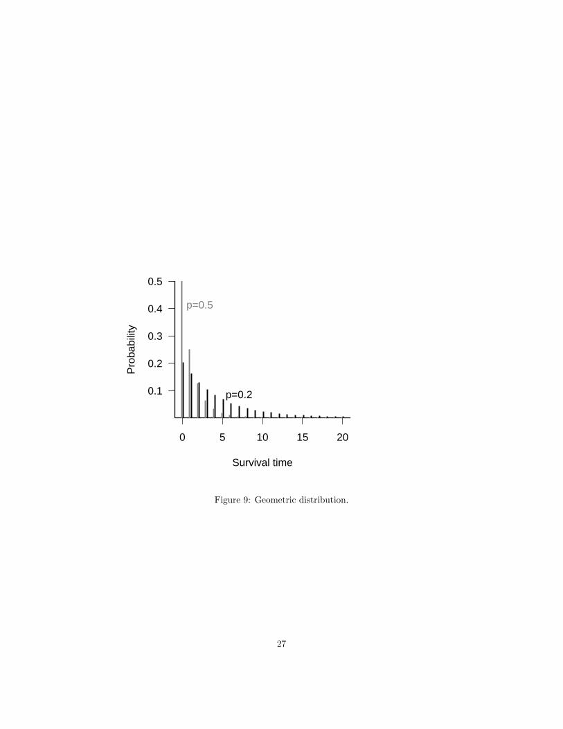
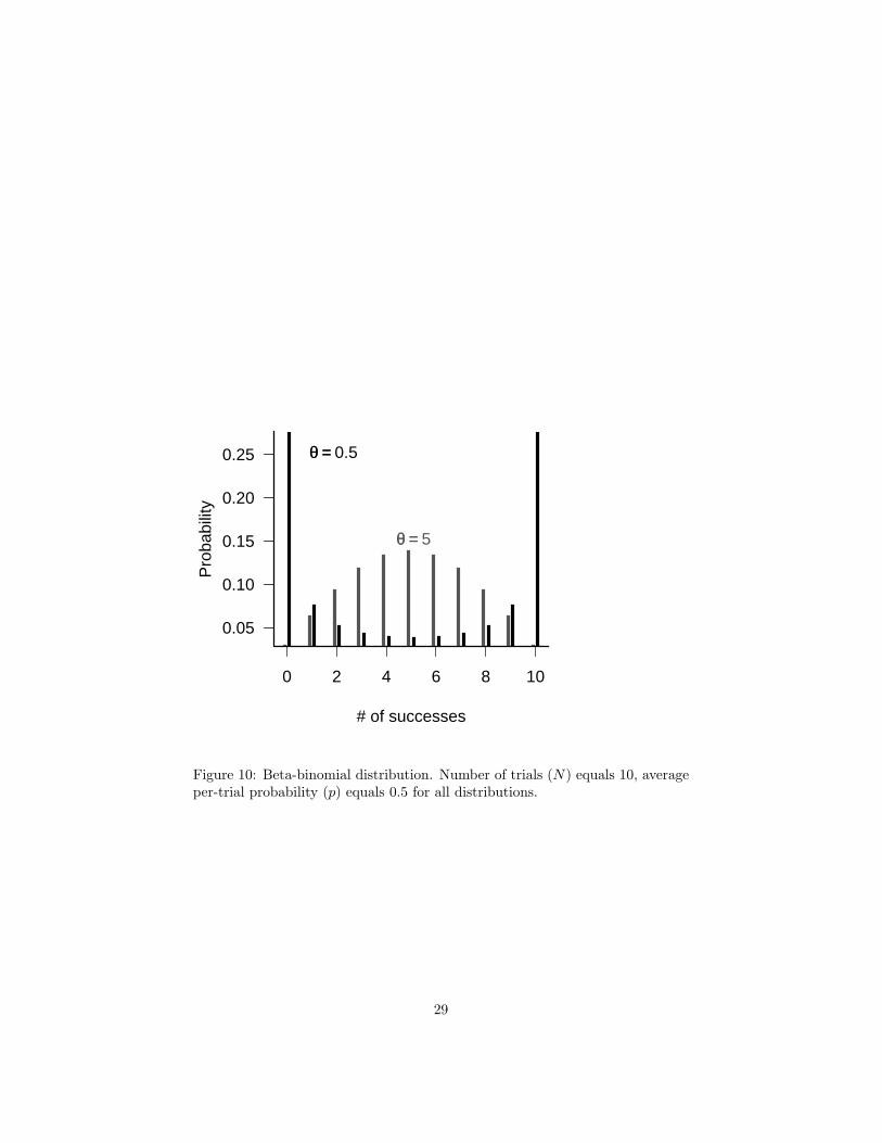
5.1.5 Beta-binomial

Just as one can compound the Poisson distribution with a Gamma to allowfor heterogeneity in rates, producing a negative binomial, one can compoundthe binomial distribution with a Beta distribution to allow for heterogeneity inper-trial probability, producing a Beta-binomial distribution (Crowder, 1978;Reeve and Murdoch, 1985; Hatfield et al., 1996). The most common parameter-ization of the beta-binomial distribution uses the binomial parameter N (trialsper sample), plus two additional parameters a and b that describe the betadistribution of the per-trial probability. When a = b = 1 the per-trial proba-bility is equally likely to be any value between 0 and 1 (the mean is 0.5), and

26

0 5 10 15 20

0.1

0.2

0.3

0.4

0.5

Survival time

Pro

babi

lity

p=0.2

p=0.5

Figure 9: Geometric distribution.

27

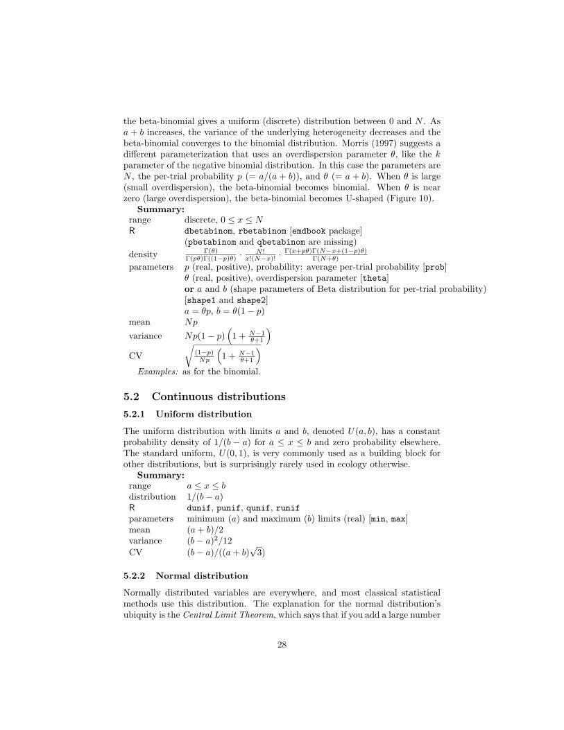
the beta-binomial gives a uniform (discrete) distribution between 0 and N . Asa + b increases, the variance of the underlying heterogeneity decreases and thebeta-binomial converges to the binomial distribution. Morris (1997) suggests adifferent parameterization that uses an overdispersion parameter θ, like the kparameter of the negative binomial distribution. In this case the parameters areN , the per-trial probability p (= a/(a + b)), and θ (= a + b). When θ is large(small overdispersion), the beta-binomial becomes binomial. When θ is nearzero (large overdispersion), the beta-binomial becomes U-shaped (Figure 10).

Summary:range discrete, 0 ≤ x ≤ NR dbetabinom, rbetabinom [emdbook package]

(pbetabinom and qbetabinom are missing)density Γ(θ)

Γ(pθ)Γ((1−p)θ) ·N !

x!(N−x)! ·Γ(x+pθ)Γ(N−x+(1−p)θ)

Γ(N+θ)

parameters p (real, positive), probability: average per-trial probability [prob]θ (real, positive), overdispersion parameter [theta]or a and b (shape parameters of Beta distribution for per-trial probability)[shape1 and shape2]a = θp, b = θ(1− p)

mean Np

variance Np(1− p)(1 + N−1

θ+1

)CV

√(1−p)

Np

(1 + N−1

θ+1

)Examples: as for the binomial.

5.2 Continuous distributions

5.2.1 Uniform distribution

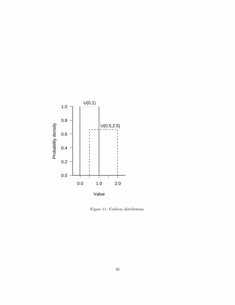
The uniform distribution with limits a and b, denoted U(a, b), has a constantprobability density of 1/(b − a) for a ≤ x ≤ b and zero probability elsewhere.The standard uniform, U(0, 1), is very commonly used as a building block forother distributions, but is surprisingly rarely used in ecology otherwise.

Summary:range a ≤ x ≤ bdistribution 1/(b− a)R dunif, punif, qunif, runifparameters minimum (a) and maximum (b) limits (real) [min, max]mean (a + b)/2variance (b− a)2/12CV (b− a)/((a + b)

√3)

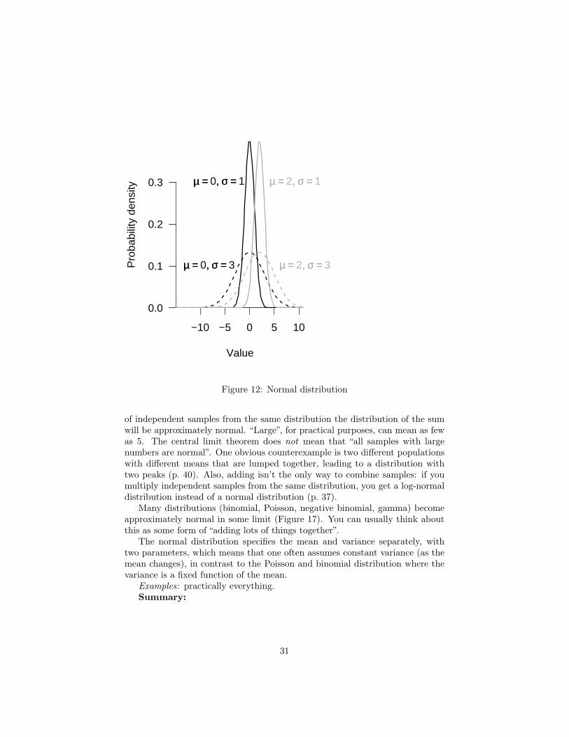
5.2.2 Normal distribution

Normally distributed variables are everywhere, and most classical statisticalmethods use this distribution. The explanation for the normal distribution’subiquity is the Central Limit Theorem, which says that if you add a large number

28

0 2 4 6 8 10

0.05

0.10

0.15

0.20

0.25

# of successes

Pro

babi

lity

θθ == 0.5

θθ == 5

Figure 10: Beta-binomial distribution. Number of trials (N) equals 10, averageper-trial probability (p) equals 0.5 for all distributions.

29

Value

Pro

babi

lity

dens

ity

0.0

0.2

0.4

0.6

0.8

1.0

0.0 1.0 2.0

U(0,1)

U(0.5,2.5)

Figure 11: Uniform distribution.

30

Value

Pro

babi

lity

dens

ity

0.0

0.1

0.2

0.3

−10 −5 0 5 10

µµ == 0,, σσ == 1

µµ == 0,, σσ == 3

µµ == 2,, σσ == 1

µµ == 2,, σσ == 3

Figure 12: Normal distribution

of independent samples from the same distribution the distribution of the sumwill be approximately normal. “Large”, for practical purposes, can mean as fewas 5. The central limit theorem does not mean that “all samples with largenumbers are normal”. One obvious counterexample is two different populationswith different means that are lumped together, leading to a distribution withtwo peaks (p. 40). Also, adding isn’t the only way to combine samples: if youmultiply independent samples from the same distribution, you get a log-normaldistribution instead of a normal distribution (p. 37).

Many distributions (binomial, Poisson, negative binomial, gamma) becomeapproximately normal in some limit (Figure 17). You can usually think aboutthis as some form of “adding lots of things together”.

The normal distribution specifies the mean and variance separately, withtwo parameters, which means that one often assumes constant variance (as themean changes), in contrast to the Poisson and binomial distribution where thevariance is a fixed function of the mean.

Examples: practically everything.Summary:

31

range all real valuesdistribution 1√

2πσexp

(− (x−µ)2

2σ2

)R dnorm, pnorm, qnorm, rnormparameters µ (real), mean [mean]

σ (real, positive), standard deviation [sd]mean µvariance σ2

CV σ/µConjugate prior Normal (µ); Gamma (1/σ2)

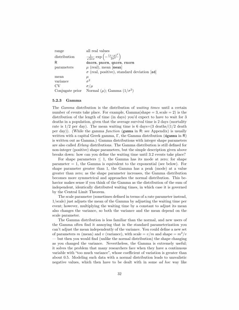
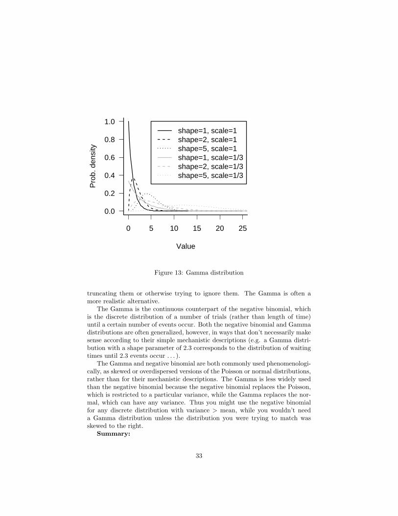
5.2.3 Gamma

The Gamma distribution is the distribution of waiting times until a certainnumber of events take place. For example, Gamma(shape = 3, scale = 2) is thedistribution of the length of time (in days) you’d expect to have to wait for 3deaths in a population, given that the average survival time is 2 days (mortalityrate is 1/2 per day). The mean waiting time is 6 days=(3 deaths/(1/2 deathper day)). (While the gamma function (gamma in R: see Appendix) is usuallywritten with a capital Greek gamma, Γ, the Gamma distribution (dgamma in R)is written out as Gamma.) Gamma distributions with integer shape parametersare also called Erlang distributions. The Gamma distribution is still defined fornon-integer (positive) shape parameters, but the simple description given abovebreaks down: how can you define the waiting time until 3.2 events take place?

For shape parameters ≤ 1, the Gamma has its mode at zero; for shapeparameter = 1, the Gamma is equivalent to the exponential (see below). Forshape parameter greater than 1, the Gamma has a peak (mode) at a valuegreater than zero; as the shape parameter increases, the Gamma distributionbecomes more symmetrical and approaches the normal distribution. This be-havior makes sense if you think of the Gamma as the distribution of the sum ofindependent, identically distributed waiting times, in which case it is governedby the Central Limit Theorem.

The scale parameter (sometimes defined in terms of a rate parameter instead,1/scale) just adjusts the mean of the Gamma by adjusting the waiting time perevent; however, multiplying the waiting time by a constant to adjust its meanalso changes the variance, so both the variance and the mean depend on thescale parameter.

The Gamma distribution is less familiar than the normal, and new users ofthe Gamma often find it annoying that in the standard parameterization youcan’t adjust the mean independently of the variance. You could define a new setof parameters m (mean) and v (variance), with scale = v/m and shape = m2/v— but then you would find (unlike the normal distribution) the shape changingas you changed the variance. Nevertheless, the Gamma is extremely useful;it solves the problem that many researchers face when they have a continuousvariable with “too much variance”, whose coefficient of variation is greater thanabout 0.5. Modeling such data with a normal distribution leads to unrealisticnegative values, which then have to be dealt with in some ad hoc way like

32

0 5 10 15 20 25

0.0

0.2

0.4

0.6

0.8

1.0

Value

Pro

b. d

ensi

ty

shape=1, scale=1shape=2, scale=1shape=5, scale=1shape=1, scale=1/3shape=2, scale=1/3shape=5, scale=1/3

Figure 13: Gamma distribution

truncating them or otherwise trying to ignore them. The Gamma is often amore realistic alternative.

The Gamma is the continuous counterpart of the negative binomial, whichis the discrete distribution of a number of trials (rather than length of time)until a certain number of events occur. Both the negative binomial and Gammadistributions are often generalized, however, in ways that don’t necessarily makesense according to their simple mechanistic descriptions (e.g. a Gamma distri-bution with a shape parameter of 2.3 corresponds to the distribution of waitingtimes until 2.3 events occur . . . ).

The Gamma and negative binomial are both commonly used phenomenologi-cally, as skewed or overdispersed versions of the Poisson or normal distributions,rather than for their mechanistic descriptions. The Gamma is less widely usedthan the negative binomial because the negative binomial replaces the Poisson,which is restricted to a particular variance, while the Gamma replaces the nor-mal, which can have any variance. Thus you might use the negative binomialfor any discrete distribution with variance > mean, while you wouldn’t needa Gamma distribution unless the distribution you were trying to match wasskewed to the right.

Summary:

33

range positive real valuesR dgamma, pgamma, qgamma, rgammadistribution 1

saΓ(a)xa−1e−x/s

parameters s (real, positive), scale: length per event [scale]or r (real, positive), rate = 1/s; rate at which events occur [rate]a (real, positive), shape: number of events [shape]

mean as or a/rvariance as2 or a/r2

CV 1/√

aExamples: almost any environmental variable with a large variance where

negative values don’t make sense: nitrogen concentrations, light intensity, etc..

5.2.4 Exponential

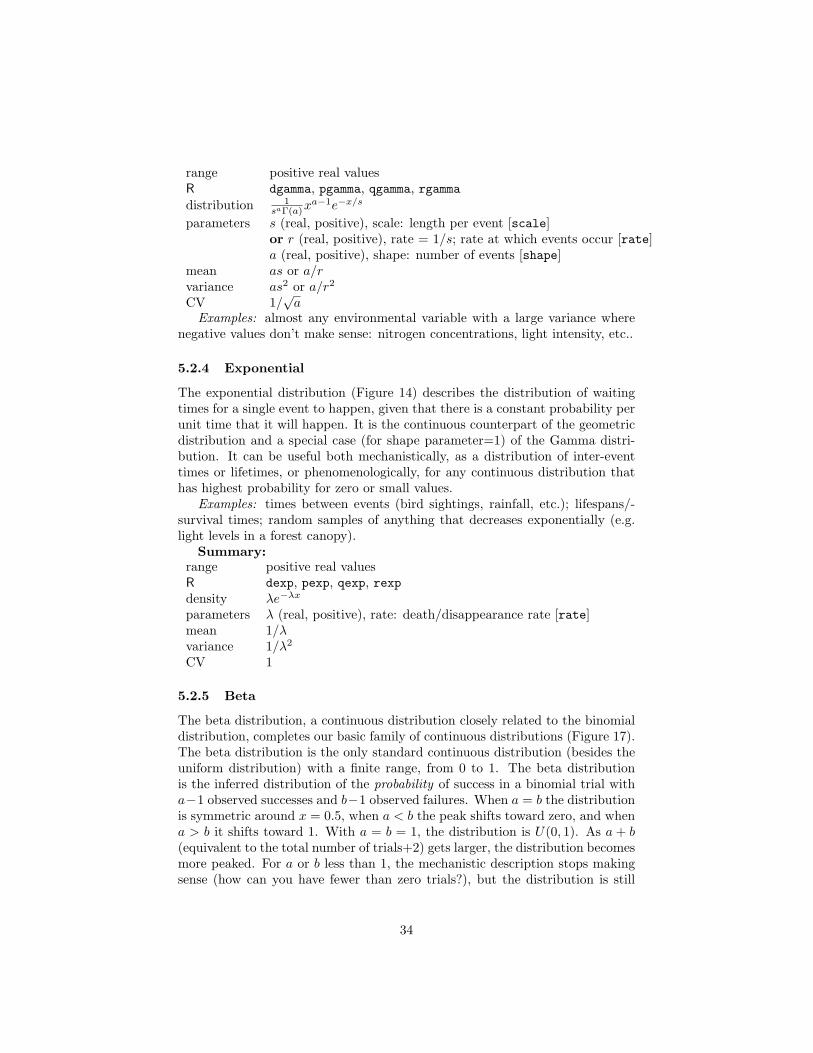
The exponential distribution (Figure 14) describes the distribution of waitingtimes for a single event to happen, given that there is a constant probability perunit time that it will happen. It is the continuous counterpart of the geometricdistribution and a special case (for shape parameter=1) of the Gamma distri-bution. It can be useful both mechanistically, as a distribution of inter-eventtimes or lifetimes, or phenomenologically, for any continuous distribution thathas highest probability for zero or small values.

Examples: times between events (bird sightings, rainfall, etc.); lifespans/-survival times; random samples of anything that decreases exponentially (e.g.light levels in a forest canopy).

Summary:range positive real valuesR dexp, pexp, qexp, rexpdensity λe−λx

parameters λ (real, positive), rate: death/disappearance rate [rate]mean 1/λvariance 1/λ2

CV 1

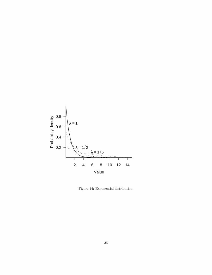
5.2.5 Beta

The beta distribution, a continuous distribution closely related to the binomialdistribution, completes our basic family of continuous distributions (Figure 17).The beta distribution is the only standard continuous distribution (besides theuniform distribution) with a finite range, from 0 to 1. The beta distributionis the inferred distribution of the probability of success in a binomial trial witha−1 observed successes and b−1 observed failures. When a = b the distributionis symmetric around x = 0.5, when a < b the peak shifts toward zero, and whena > b it shifts toward 1. With a = b = 1, the distribution is U(0, 1). As a + b(equivalent to the total number of trials+2) gets larger, the distribution becomesmore peaked. For a or b less than 1, the mechanistic description stops makingsense (how can you have fewer than zero trials?), but the distribution is still

34

2 4 6 8 10 12 14

0.2

0.4

0.6

0.8

Value

Pro

babi

lity

dens

ity

λλ == 1

λλ == 1 2λλ == 1 5

Figure 14: Exponential distribution.

35

0.0 0.2 0.4 0.6 0.8 1.0

0

1

2

3

4

5

Value

Pro

babi

lity

dens

ity

a=1, b=5

a=5, b=5

a=5, b=1

a=0.5, b=0.5

a=1, b=1

Figure 15: Beta distribution

well-defined, and when a and b are both between 0 and 1 it becomes U-shaped— it has peaks at p = 0 and p = 1.

The beta distribution is obviously good for modeling probabilities or propor-tions. It can also be useful for modeling continuous distributions with peaks atboth ends, although in some cases a finite mixture model (p. 40) may be moreappropriate. The beta distribution is also useful whenever you have to definea continuous distribution on a finite range, as it is the only such standard con-tinuous distribution. It’s easy to rescale the distribution so that it applies oversome other finite range instead of from 0 to 1: for example, Tiwari et al. (2005)used the beta distribution to describe the distribution of turtles on a beach, sothe range would extend from 0 to the length of the beach.

Summary:

36

range real, 0 to 1R dbeta, pbeta, qbeta, rbetadensity Γ(a+b)

Γ(a)Γ(b)xa−1(1− x)b−1

parameters a (real, positive), shape 1: number of successes +1 [shape1]b (real, positive), shape 2: number of failures +1 [shape2]

mean a/(a + b)mode (a− 1)/(a + b− 2)variance ab/((a + b)2)(a + b + 1)CV

√(b/a)/(a + b + 1)

5.2.6 Lognormal

The lognormal falls outside the neat classification scheme we’ve been buildingso far; it is not the continuous analogue or limit of some discrete sampling distri-bution (Figure 17)∗. Its mechanistic justification is like the normal distribution(the Central Limit Theorem), but for the product of many independent, identi-cal variates rather than their sum. Just as taking logarithms converts productsinto sums, taking the logarithm of a lognormally distributed variable—whichmight result from the product of independent variables—converts it it into anormally distributed variable resulting from the sum of the logarithms of thoseindependent variables. The best example of this mechanism is the distributionof the sizes of individuals or populations that grow exponentially, with a percapita growth rate that varies randomly over time. At each time step (daily,yearly, etc.), the current size is multiplied by the randomly chosen growth in-crement, so the final size (when measured) is the product of the initial size andall of the random growth increments.

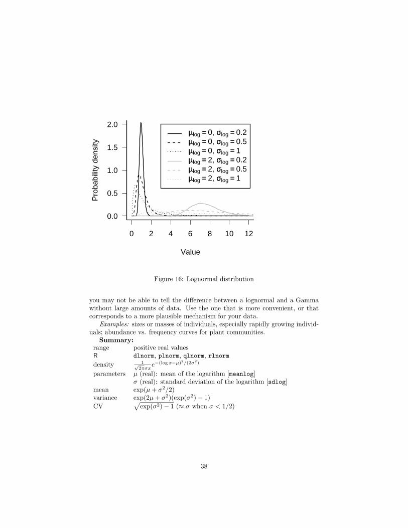
One potentially puzzling aspect of the lognormal distribution is that its meanis not what you might naively expect if you exponentiate a normal distributionwith mean µ (i.e. eµ). Because of Jensen’s inequality, and because the exponen-tial function is an accelerating function, the mean of the lognormal, eµ+σ2/2, isgreater than eµ by an amount that depends on the variance of the original nor-mal distribution. When the variance is small relative to the mean, the mean isapproximately equal to eµ, and the lognormal itself looks approximately normal(e.g. solid lines in Figure 16, with σ(log) = 0.2). As with the Gamma distri-bution, the distribution also changes shape as the variance increases, becomingmore skewed.

The log-normal is also used phenomenologically in some of the same situa-tions where a Gamma distribution also fits: continuous, positive distributionswith long tails or variance much greater than the mean (McGill et al., 2006).Like the distinction between a Michaelis-Menten and a saturating exponential,

∗The lognormal extends our table in another direction — exponential transformation of aknown distribution. Other distributions have this property, most notably the extreme valuedistribution, which is the log-exponential: if Y is exponentially distributed, then log Y isextreme-value distributed. As its name suggests, the extreme value distribution occurs mech-anistically as the distribution of extreme values (e.g. maxima) of samples of other distributions(Katz et al., 2005).

37

0 2 4 6 8 10 12

0.0

0.5

1.0

1.5

2.0

Value

Pro

babi

lity

dens

ity

µµlog == 0, σσlog == 0.2µµlog == 0, σσlog == 0.5µµlog == 0, σσlog == 1µµlog == 2, σσlog == 0.2µµlog == 2, σσlog == 0.5µµlog == 2, σσlog == 1

Figure 16: Lognormal distribution

you may not be able to tell the difference between a lognormal and a Gammawithout large amounts of data. Use the one that is more convenient, or thatcorresponds to a more plausible mechanism for your data.

Examples: sizes or masses of individuals, especially rapidly growing individ-uals; abundance vs. frequency curves for plant communities.

Summary:range positive real valuesR dlnorm, plnorm, qlnorm, rlnormdensity 1√

2πσxe−(log x−µ)2/(2σ2)

parameters µ (real): mean of the logarithm [meanlog]σ (real): standard deviation of the logarithm [sdlog]

mean exp(µ + σ2/2)variance exp(2µ + σ2)(exp(σ2)− 1)CV

√exp(σ2)− 1 (≈ σ when σ < 1/2)

38

large N,small p

uniform

geometric

Poisson

large k

k=1

binomiallarge N,

intermediate p

normal

lognormal

shape=1

exponential

log/exp

large shape

large λ

gamma

beta

a and b large

beta−binomial

large θ a=b=1

negative binomial

transform

conjugate priors

limit / special case

DISCRETE CONTINUOUS

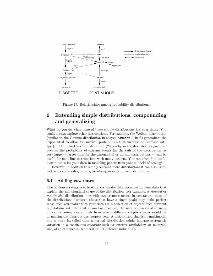
Figure 17: Relationships among probability distributions.

6 Extending simple distributions; compoundingand generalizing

What do you do when none of these simple distributions fits your data? Youcould always explore other distributions. For example, the Weibull distribution(similar to the Gamma distribution in shape: ?dweibull in R) generalizes theexponential to allow for survival probabilities that increase or decrease withage (p. ??). The Cauchy distribution (?dcauchy in R), described as fat-tailedbecause the probability of extreme events (in the tails of the distribution) isvery large — larger than for the exponential or normal distributions — can beuseful for modeling distributions with many outliers. You can often find usefuldistributions for your data in modeling papers from your subfield of ecology.

However, in addition to simply learning more distributions it can also usefulto learn some strategies for generalizing more familiar distributions.

6.1 Adding covariates

One obvious strategy is to look for systematic differences within your data thatexplain the non-standard shape of the distribution. For example, a bimodal ormultimodal distribution (one with two or more peaks, in contrast to most ofthe distributions discussed above that have a single peak) may make perfectsense once you realize that your data are a collection of objects from differentpopulations with different means.For example, the sizes or masses of sexuallydimorphic animals or animals from several different cryptic species would bi-or multimodal distributions, respectively. A distribution that isn’t multimodalbut is more fat-tailed than a normal distribution might indicate systematicvariation in a continuous covariate such as nutrient availability, or maternalsize, of environmental temperature, of different individuals.

39

6.2 Mixture models

But what if you can’t identify systematic differences? You can still extendstandard distributions by supposing that your data are really a mixture of ob-servations from different types of individuals, but that you can’t observe the(finite) types or (continuous) covariates of individuals. These distributions arecalled mixture distributions or mixture models. Fitting them to data can bechallenging, but they are very flexible.

6.2.1 Finite mixtures

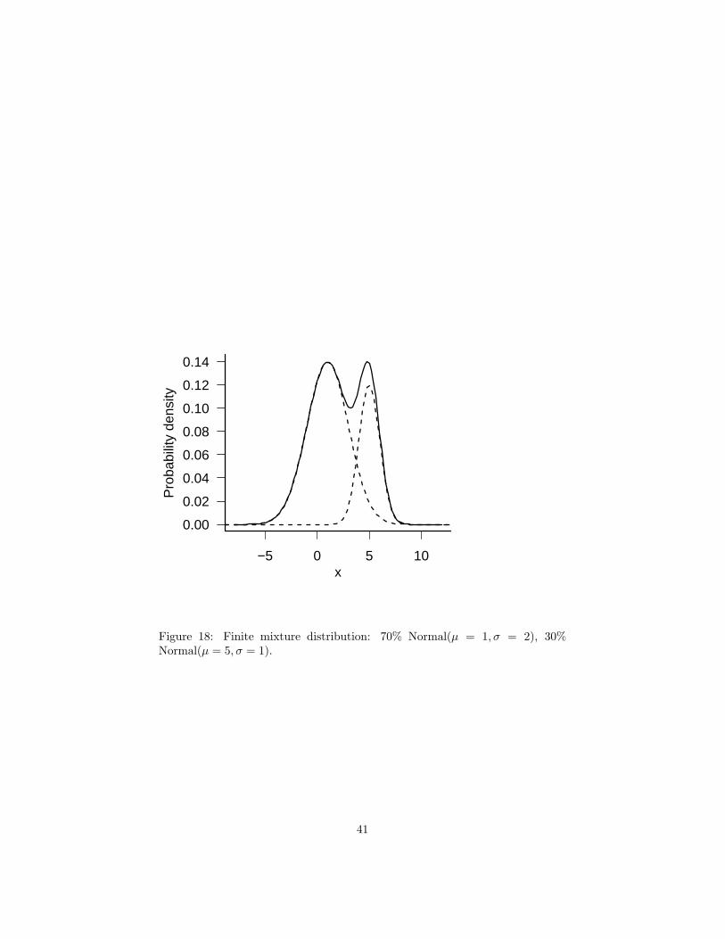
Finite mixture models suppose that your observations are drawn from a discreteset of unobserved categories, each of which has its own distribution: typically allcategories have the same type of distribution, such as normal, but with differentmean or variance parameters. Finite mixture distributions often fit multimodaldata. Finite mixtures are typically parameterized by the parameters of eachcomponent of the mixture, plus a set of probabilities or percentages describingthe amount of each component. For example, 30% of the organisms (p = 0.3)could be in group 1, normally distributed with mean 1 and standard deviation2, while 70% (1 − p = 0.7) are in group 2, normally distributed with mean5 and standard deviation 1 (Figure 18). If the peaks of the distributions arecloser together, or their standard deviations are larger so that the distributionsoverlap, you’ll see a broad (and perhaps lumpy) peak rather than two distinctpeaks.

Zero-inflated models are a common type of finite mixture model (Inouye,1999; Martin et al., 2005). Zero-inflated models (Figure 1). combine a standarddiscrete probability distribution (e.g. binomial, Poisson, or negative binomial),which typically include some probability of sampling zero counts even whensome individuals are present, with some additional process that can also lead toa zero count (e.g. complete absence of the species or trap failure).

6.3 Continuous mixtures

Continuous mixture distributions, also known as compounded distributions, al-low the parameters themselves to vary randomly, drawn from their own distri-bution. They are a sensible choice for overdispersed data, or for data where yoususpect that unobserved covariates may be important. Technically, compoundeddistributions are the distribution of a sampling distribution S(x, p) with param-eter(s) p that vary according to another (typically continuous) distribution P (p).The distribution of the compounded distribution C is C(x) =

∫S(x, p)P (p)dp.

For example, compounding a Poisson distribution by drawing the rate parame-ter λ from a Gamma distribution with shape parameter k (and scale parameterλ/k, to make the mean equal to λ) results in a negative binomial distribution(p. 22). Continuous mixture distributions are growing ever more popular inecology as ecologists try to account for heterogeneity in their data.

The negative binomial, which could also be called the Gamma-Poisson dis-tribution to highlight its compound origin, is the most common compounded

40

−5 0 5 10

0.00

0.02

0.04

0.06

0.08

0.10

0.12

0.14

Pro

babi

lity

dens

ity

x

Figure 18: Finite mixture distribution: 70% Normal(µ = 1, σ = 2), 30%Normal(µ = 5, σ = 1).

41

distribution. The Beta-binomial is also fairly common: like the negative bi-nomial, it compounds a common discrete distribution (binomial) with its con-jugate prior (Beta), resulting in a mathematically simple form that allows formore variability. The lognormal-Poisson is very similar to the negative bino-mial, except that (as its name suggests) it uses the lognormal instead of theGamma as a compounding distribution. One technical reason to use the lesscommon lognormal-Poisson is that on the log scale the rate parameter is nor-mally distributed, which simplifies some numerical procedures (Elston et al.,2001).

Clark et al. (1999) used the Student t distribution to model seed disper-sal curves. Seeds often disperse fairly uniformly near parental trees but alsohave a high probability of long dispersal. These two characteristics are incom-patible with standard seed dispersal models like the exponential and normaldistributions. Clark et al. assumed that the seed dispersal curve represents acompounding of a normal distribution for the dispersal of any one seed with anGamma distribution of the inverse variance of the distribution of any particularseed (i.e., 1/σ2 ∼ Gamma)∗. This variation in variance accounts for the differ-ent distances that different seeds may travel as a function of factors like theirsize, shape, height on the tree, and the wind speed at the time they are released.Clark et al. used compounding to model these factors as random, unobservedcovariates since they are practically impossible to measure for all the individualseeds on a tree or in a forest.

The inverse Gamma-normal model is equivalent to the Student t distribu-tion, which you may recognize from t tests in classical statistics and whichstatisticians sometimes use as a phenomenological model for fat-tailed distribu-tions. Clark et al. extended the usual one-dimensional t distribution (?dt inR) to the two-dimensional distribution of seeds around a parent and called itthe 2Dt distribution. The 2Dt distribution has a scale parameter that deter-mines the mean dispersal distance and a shape parameter p. When p is largethe underlying Gamma distribution has a small coefficient of variation and the2Dt distribution is close to normal; when p = 1 the 2Dt becomes a Cauchydistribution.

Generalized distributions are an alternative class of mixture distribution thatarises when there is a sampling distribution S(x) for the number of individualswithin a cluster and another sampling distribution C(x) for number of clustersin a sampling unit. For example, the distribution of number of eggs per squaremight be generalized from the distribution of clutches per square and of eggsper clutch. A standard example is the “Poisson-Poisson” or “Neyman Type A”distribution (Pielou, 1977), which assumes a Poisson distribution of clusterswith a Poisson distribution of individuals in each.

Figuring out the probability distribution or density formulas for compoundeddistributions analytically is mathematically challenging (see Bailey (1964) orPielou (1977) for the gory details), but R can easily generate random numbers

∗This choice of a compounding distribution, which may seem arbitrary, turns out to bemathematically convenient.

42

from these distributions (see the R supplement for more detail).The key is that R’s functions for generating random distributions (rpois,

rbinom, etc.) can take vectors for their parameters. Rather than generate(say) 20 deviates from a binomial distribution with N trials and and a fixedper-trial probability p, you can choose 20 deviates with N trials and a vectorof 20 different per-trial probabilities p1 to p20. Furthermore, you can gener-ate this vector of parameters from another randomizing function! For example,to generate 20 beta-binomial deviates with N = 10 and the per-trial proba-bilities drawn from a beta distribution with a = 2 and b = 1, you could userbinom(20,rbeta(20,2,1)).

Compounding and generalizing are powerful ways to extend the range ofstochastic ecological models. A good fit to a compounded distribution also sug-gests that environmental variation is shaping the variation in the population.But be careful: Pielou (1977) demonstrates that for Poisson distributions, everygeneralized distribution (corresponding to variation in the underlying density)can also be generated by a compound distribution (corresponding to individualsoccurring in clusters), and concludes that (p. 123) “the fitting of theoretical fre-quency distributions to observational data can never by itself suffice to ‘explain’the pattern of a natural population”.

43

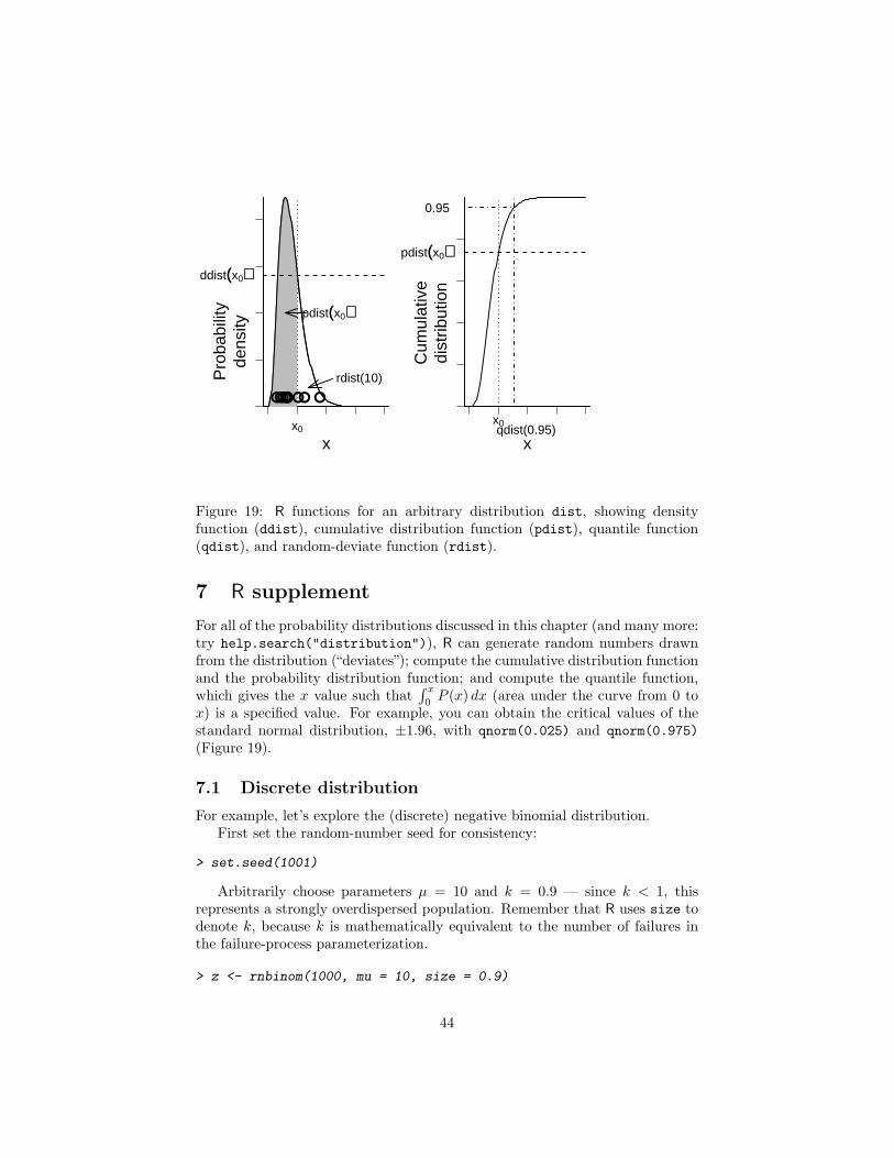
xx0

ddist((x0))

pdist((x0))

Pro

babi

lity

dens

ity

●● ●●●●● ●●●

rdist(10)

x

x0

pdist((x0))

0.95

qdist(0.95)C

umul

ativ

edi

strib

utio

n

Figure 19: R functions for an arbitrary distribution dist, showing densityfunction (ddist), cumulative distribution function (pdist), quantile function(qdist), and random-deviate function (rdist).

7 R supplement

For all of the probability distributions discussed in this chapter (and many more:try help.search("distribution")), R can generate random numbers drawnfrom the distribution (“deviates”); compute the cumulative distribution functionand the probability distribution function; and compute the quantile function,which gives the x value such that

∫ x

0P (x) dx (area under the curve from 0 to

x) is a specified value. For example, you can obtain the critical values of thestandard normal distribution, ±1.96, with qnorm(0.025) and qnorm(0.975)(Figure 19).

7.1 Discrete distribution

For example, let’s explore the (discrete) negative binomial distribution.First set the random-number seed for consistency:

> set.seed(1001)

Arbitrarily choose parameters µ = 10 and k = 0.9 — since k < 1, thisrepresents a strongly overdispersed population. Remember that R uses size todenote k, because k is mathematically equivalent to the number of failures inthe failure-process parameterization.

> z <- rnbinom(1000, mu = 10, size = 0.9)

44

Check the first few values:

> head(z)

[1] 41 3 3 0 11 14

Since the negative binomial has no set upper limit, we will just plot theresults up to the maximum value sampled:

> maxz <- max(z)

The easiest way to plot the results is:

> f <- factor(z, levels = 0:maxz)

> plot(f)

using the levels specification to make sure that all values up to the maxi-mum are included in the plot even when none were sampled in this particularexperiment.

If we want the observed probabilities (freq/N) rather than the frequencies:

> obsprobs <- table(f)/1000

> plot(obsprobs)

Add theoretical values:

> tvals <- dnbinom(0:maxz, size = 0.9, mu = 10)

> points(0:maxz, tvals)

You could plot the deviations with plot(0:maxz,obsprobs-tvals); thisgives you some idea how the variability changes with the mean.

Find the probability that x > 30:

> pnbinom(30, size = 0.9, mu = 10, lower.tail = FALSE)

[1] 0.05725252

By default R’s distribution functions will give you the lower tail of the distri-bution — the probability that x is less than or equal to some particular value.You could use 1-pnbinom(30,size=0.9,mu=10) to get the uppper tail sinceProb(x > 30) = 1 − Prob(x ≤ 30), but using lower.tail=FALSE to get theupper tail is more numerically accurate.

What is the upper 95th percentile of the distribution?

> qnbinom(0.95, size = 0.9, mu = 10)

[1] 32

To get the lower and upper 95% confidence limits, you need

> qnbinom(c(0.025, 0.975), size = 0.9, mu = 10)

45

[1] 0 40

You can also use the random sample z to check that the mean and variance,and 95th quantile of the sample, agree reasonably well with the theoreticalexpectations:

> mu <- 10

> k <- 0.9

> c(mu, mean(z))

[1] 10.000 9.654

> c(mu * (1 + mu/k), var(z))

[1] 121.1111 113.6539

> c(qnbinom(0.95, size = k, mu = mu), quantile(z, 0.95))

95%32 31

7.2 Continuous distribution: lognormal

Going through the same exercise for the lognormal, a continuous distribution:

> z <- rlnorm(1000, meanlog = 2, sdlog = 1)

Plot the results:

> hist(z, breaks = 100, freq = FALSE)

> lines(density(z, from = 0), lwd = 2)

Add theoretical values:

> curve(dlnorm(x, meanlog = 2, sdlog = 1), add = TRUE,

+ lwd = 2, from = 0, col = "darkgray")

The probability of x > 20, 95% confidence limits:

> plnorm(30, meanlog = 2, sdlog = 1, lower.tail = FALSE)

[1] 0.08057753

> qlnorm(c(0.025, 0.975), meanlog = 2, sdlog = 1)

[1] 1.040848 52.455437

Comparing the theoretical values given on p. 38 with the observed values forthis random sample:

46

Distribution Type Range Skew ExamplesBinomial Discrete 0, N any Number surviving, number killedPoisson Discrete 0,∞ right → none Seeds per quadrat, settlers (vari-

ance/mean ≈ 1)Negative binomial Discrete 0,∞ right Seeds per quadrat, settlers (vari-

ance/mean > 1)Geometric Discrete 0,∞ right Discrete lifetimesNormal Continuous −∞,∞ none MassGamma Continuous 0,∞ right Survival time, distance to nearest

edgeExponential Continuous 0,∞ right Survival time, distance to nearest

edgeLognormal Continuous 0,∞ right Size, mass (exponential growth)

Table 1: Summary of probability distributions

> meanlog <- 2

> sdlog <- 1

> c(exp(meanlog + sdlog^2/2), mean(z))

[1] 12.18249 12.12708

> c(exp(2 * meanlog + sdlog^2) * (exp(sdlog^2) - 1),

+ var(z))

[1] 255.0156 184.7721

> c(qlnorm(0.95, meanlog = meanlog, sdlog = sdlog),

+ quantile(z, 0.95))

95%38.27717 39.65172

There is a fairly large difference between the expected and observed variance.This is typical: variances of random samples have larger variances, or abso-lute differences from their theoretical expected values, than means of randomsamples.

Sometimes it’s easier to deal with log-normal data by taking the logarithmof the data and comparing them to the normal distribution:

> hist(log(z), freq = FALSE, breaks = 100)

> curve(dnorm(x, mean = meanlog, sd = sdlog), add = TRUE,

+ lwd = 2)

47

7.3 Mixing and compounding distributions

7.3.1 Finite mixture distributions

The general recipe for generating samples from finite mixtures is to use a uniformdistribution to sample which of the components of the mixture to sample, thenuse ifelse to pick values from one distribution or the other. To pick 1000 valuesfrom a mixture of normal distributions with the parameters shown in Figure 18(p = 0.3, µ1 = 1, σ1 = 2, µ2 = 5, σ2 = 1):

> u1 <- runif(1000)

> z <- ifelse(u1 < 0.3, rnorm(1000, mean = 1, sd = 2),

+ rnorm(1000, mean = 5, sd = 1))

> hist(z, breaks = 100, freq = FALSE)

The probability density of a finite mixture composed of two distributions D1

and D2 in proportions p1 and 1− p1 is p1D1 + p2D2. We can superimpose thetheoretical probability density for the finite mixture above on the histogram:

> curve(0.3 * dnorm(x, mean = 1, sd = 2) + 0.7 * dnorm(x,

+ mean = 5, sd = 1), add = TRUE, lwd = 2)

The general formula for the probability distribution of a zero-inflated distri-bution, with an underlying distribution P (x) and a zero-inflation probability ofpz, is:

Prob(0) = pz + (1− pz)P (0)Prob(x > 0) = (1− pz)P (x)

So, for example, we could define a probability distribution for a zero-inflatednegative binomial as follows:

> dzinbinom = function(x, mu, size, zprob) {

+ ifelse(x == 0, zprob + (1 - zprob) * dnbinom(0,

+ mu = mu, size = size), (1 - zprob) * dnbinom(x,

+ mu = mu, size = size))

+ }

(the name, dzinbinom, follows the R convention for a probability distributionfunction: a d followed by the abbreviated name of the distribution, in this casezinbinom for “zero-inflated negative binomial”).

The ifelse command checks every element of x to see whether it is zero ornot and fills in the appropriate value depending on the answer.

Here’s a random deviate generator:

> rzinbinom = function(n, mu, size, zprob) {

+ ifelse(runif(n) < zprob, 0, rnbinom(n, mu = mu,

+ size = size))

+ }

48

The command runif(n) picks n random values between 0 and 1; the ifelsecommand compares them with the value of zprob. If an individual value is lessthan zprob (which happens with probability zprob=pz), then the correspondingrandom number is zero; otherwise it is a value picked out of the appropriatenegative binomial distribution.

7.3.2 Compounded distributions

Start by confirming numerically that a negative binomial distribution is reallya compounded Poisson-Gamma distribution. Pick 1000 values out of a Gammadistribution, then use those values as the λ (rate) parameters in a random drawfrom a Poisson distribution:

> k <- 3

> mu <- 10

> lambda <- rgamma(1000, shape = k, scale = mu/k)

> z <- rpois(1000, lambda)

> P1 <- table(factor(z, levels = 0:max(z)))/1000

> plot(P1)

> P2 <- dnbinom(0:max(z), mu = 10, size = 3)

> points(0:max(z), P2)

Establish that a Poisson-lognormal and a Poisson-Gamma (negative bino-mial) are not very different: pick the Poisson-lognormal with approximately thesame mean and variance as the negative binomial just shown.

> mlog <- mean(log(lambda))

> sdlog <- sd(log(lambda))

> lambda2 <- rlnorm(1000, meanlog = mlog, sdlog = sdlog)

> z2 <- rpois(1000, lambda2)

> P3 <- table(factor(z2, levels = 0:max(z)))/1000

> matplot(0:max(z), cbind(P1, P3), pch = 1:2)

> lines(0:max(z), P2)

References

Bailey, N. T. J. 1964. The elements of Stochastic Processes with applicationsto the natural sciences. Wiley, New York.

Bjørnstad, O. N. and B. T. Grenfell. 2001. Noisy clockwork: Time series analysisof population fluctuations in animals. Science 293:638–643.

Bradlow, E. T., B. G. S. Hardie, and P. S. Fader. 2002. Bayesian inferencefor the negative binomial distribution via polynomial expansions. Journal ofComputational & Graphical Statistics 11:189–201.

Brown, D. H. and B. M. Bolker. 2004. The effects of disease dispersal andhost clustering on the epidemic threshold in plants. Bulletin of MathematicalBiology 66:341–371.

49

Clark, J. S., M. Silman, R. Kern, E. Macklin, and J. HilleRisLambers. 1999.Seed dispersal near and far: patterns across temperate and tropical forests.Ecology 80:1475–1494.

Crome, F. H. J., M. R. Thomas, and L. A. Moore. 1996. A novel Bayesianapproach to assessing impacts of rain forest logging. Ecological Applications6:1104–1123.

Crowder, M. J. 1978. Beta-binomial Anova for proportions. Applied Statistics27:34–37.

Dennis, B. 1996. Discussion: Should ecologists become Bayesians? EcologicalApplications 6:1095–1103.

Diaconis, P., S. Holmes, and R. Montgomery. 2004. Dynamical bias in the cointoss. URL http://www-stat.stanford.edu/reports/abstracts/04-32.pdf. Technical report #2004-32, Stanford University.

Edwards, D. 1996. Comment: The first data analysis should be journalistic.Ecological Applications 6:1090–1094.

Ellison, A. M. 1996. An introduction to Bayesian inference for ecological researchand environmental decision-making. Ecological Applications 6:1036–1046.

Elston, D. A., R. Moss, T. Boulinier, C. Arrowsmith, and X. Lambin. 2001.Analysis of aggregation, a worked example: numbers of ticks on red grousechicks. Parasitology 122:563–569.

Evans, M., N. Hastings, and B. Peacock. 2000. Statistical Distributions. Wiley,New York. 3d edition.

Gelman, A., J. Carlin, H. S. Stern, and D. B. Rubin. 1996. Bayesian dataanalysis. Chapman and Hall, New York, New York, USA.

Gelman, A. and D. Nolan. 2002. You can load a die, but you can’t bias a coin.The American Statistician 56:308–311.

Hatfield, J. S., W. A. Link, D. K. Dawson, and E. L. Lindquist. 1996. Coexis-tence and community structure of tropical trees in a Hawaiian montane rainforest. Biotropica 28:746–758.

Hilborn, R. and M. Mangel. 1997. The Ecological Detective : confronting modelswith data. Princeton University Press, Princeton, New Jersey, USA.

Inouye, B. D. 1999. Estimating competition coefficients: strong competitionamong three species of frugivorous flies. Oecologia 120:588–594.

—. 2005. The importance of the variance around the mean effect size of ecologicalprocesses: comment. Ecology 86:262–264.

50

Katz, R. W., G. S. Brush, and M. B. Parlange. 2005. Statistics of extremes:Modeling ecological disturbances. Ecology 86:112–1134.

Martin, T. G., B. A. Wintle, J. R. Rhodes, P. M. Kuhnert, S. A. Field, S. A.Low-Choy, A. J. Tyre, and H. H. Possingham. 2005. Zero-tolerance ecology:improving ecological inference by modelling the source of zero observations.Ecology Letters 8:1235–1246.

May, R. M. 1978. Host-parasitoid systems in patchy environments: A phe-nomenological model. Journal of Animal Ecology 47:833–844.

McGill, B. J., B. A. Maurer, and M. D. Weiser. 2006. Empirical evaluation ofneutral theory. Ecology 87:1411–1423.

Morris, W. F. 1997. Disentangling effects of induced plant defenses and foodquantity on herbivores by fitting nonlinear models. American Naturalist150:299–327.

Pielou, E. 1977. Mathematical Ecology. Wiley, New York. 2d edition.

Rand, D. A. and H. B. Wilson. 1991. Chaotic stochasticity: a ubiquitous sourceof unpredictability in epidemics. Proceedings of the Royal Society, B 246:6.

Reeve, J. D. and W. W. Murdoch. 1985. Aggregation by parasitoids in thesuccessful control of the California red scale: A test of theory. Journal ofAnimal Ecology 54:797–816.

Ruel, J. J. and M. P. Ayres. 1999. Jensen’s inequality predicts effects of envi-ronmental variation. Trends in Ecology and Evolution 14:361–366.

Shaw, D. J. and A. P. Dobson. 1995. Patterns of macroparasite abundance andaggregation in wildlife populations: a quantitative review. Parasitology 111Suppl:S111–S127.

Tiwari, M., K. A. Bjorndal, A. B. Bolten, and B. M. Bolker. 2005. Intraspecificapplication of the mid-domain effect model: spatial and temporal nest distri-butions of green turtles, Chelonia mydas, at Tortuguero, Costa Rica. EcologyLetters 8:918–924.

Tyre, A. J., B. Tenhumberg, S. A. Field, D. Niejalke, K. Parris, and H. P. Poss-ingham. 2003. Improving precision and reducing bias in biological surveys:estimating false-negative error rates. Ecological Applications 13:1790–1801.

51