computer-aided multiscale modelling for chemical …computer-aided multiscale modelling for chemical...
TRANSCRIPT

General rights Copyright and moral rights for the publications made accessible in the public portal are retained by the authors and/or other copyright owners and it is a condition of accessing publications that users recognise and abide by the legal requirements associated with these rights.
Users may download and print one copy of any publication from the public portal for the purpose of private study or research.
You may not further distribute the material or use it for any profit-making activity or commercial gain
You may freely distribute the URL identifying the publication in the public portal If you believe that this document breaches copyright please contact us providing details, and we will remove access to the work immediately and investigate your claim.
Downloaded from orbit.dtu.dk on: Apr 16, 2020
Computer-Aided Multiscale Modelling for Chemical Product-Process Design
Morales Rodriguez, Ricardo
Publication date:2009
Document VersionPublisher's PDF, also known as Version of record
Link back to DTU Orbit
Citation (APA):Morales Rodriguez, R. (2009). Computer-Aided Multiscale Modelling for Chemical Product-Process Design. Kgs.Lyngby, Denmark: Technical University of Denmark.

Computer-Aided Multiscale
Modelling for Chemical Product-
Process Design
Ph. D. Thesis
Ricardo Morales-Rodríguez
April 2009
Computer Aided Process-Product Engineering Center
Department of Chemical and Biochemical Engineering
Technical University of Denmark


i
Preface
This thesis is submitted as partial fulfilment of the requirements for the Ph.D.-degree at Danmarks Tekniske Universitet (Technical University of Denmark). The work has been carried out in the Computer Aided Process-Product Engineering Center (CAPEC) at Institut for Kemiteknik (Department of Chemical and Biochemical Engineering) from February 2006 to February 2009 under the supervision of Professor Rafiqul Gani and funded by Danmarks Tekniske Universitet (DTU) that is highly appreciated.
I would like to thank my supervisor for granting me the opportunity to work on this project, and for the time dedicated to the work, as well as the guidance and discussions during the development of this project.
I want to thank Dr. Peter Mathias Harper, Dr. Eduardo S. Perez Cisneros and Dr. Krist Gernaey for the comments and critics to this PhD thesis.
I also want to thank Dr. Michael Pinsky (Firmenich), Dr. Gordon Bell (Syngenta), Alain Vacher, Stéphane Déchelotte and Olivier Baudouin (ProSim) and Professor Ian Cameron (The University of Queensland) for allowing me the opportunity to have a collaboration with all of them in the development of the project.
I would like to thank the co-workers at CAPEC who I had the opportunity to work with and have so many discussion about different topics: Hugo E. González, Martin, Jakob, Elisa, Kavitha, Alicia, Axel, Ravendra; Especially to Ana Carvalho, Paloma, A., Oscar, P. and Merlin, A. (fantastic five) for all the funny time that we had besides the work.
To my friend out of CAPEC: Hector del Angel and Signe Munck for taking me out of thinking only about work; and of course, all the people that I had the opportunity to meet with them: Julia, Anne, Maja, Hannah, Martin, Iben, Signe, Aslak,…. I do not have enough space to write all your names...but you know that you are in my mind.!
My Mexican support; Jazmin G. Reyes, Luis A. Blas, Divanery Rodriguez G., Ana Laura Corso, Magui, Roberto (Bob), Ines, Naty González, Ing. Dora Espinosa Corzo, Brissa, …thanks for believing in me and your patience..!!
I want to have a special thanks to my lovely parents Adela Rodríguez and Vicente Morales who supported me during the different stages of the time spent in the development of this project: Muchas gracias Papás, los quiero mucho..!!


iii
Abstract In the past, research in chemical engineering was more focused on the design, operation and optimization of the process, such as, petrochemicals and derivates (refineries, polymer plants, etc.). The main research goal usually was the efficient production of specific low-value but high-volume commodity chemicals. Product quality in this case was defined usually by its purity rather than its molecular structure. In the recent years, however, there has been an increased interest in product centric process design, operation, monitoring and control. There has also been a shift from process design, from low-value commodity chemicals to high-value structured/special chemicals and, from continuous to batch to hybrid processes. A noticeable feature of chemical product-centric process design is that the end-use (macro-scale) properties of the product-process define the design/control of the process, while the structure properties (micro-scale) define the design and performance of the product. For this reason a multiscale approach (from the modelling or experimental design point of view) has an important role in the management of the desired end-use characteristics of the product to be developed. From a model based design (virtual) of the product, the use of multiscale models is essential in the preliminary design of the product, giving to the designer the capability to perform virtual experiments for the established work-flow (design steps). The use of mathematical models in general, and multiscale models in particular, imply the handling of complex models represented by sets of highly nonlinear partial- and ordinary- differential equations, and, algebraic equations. In virtual product design, properties at various scales need to be handled together with the mass, energy and/or momentum balance equations of different scales. That is, managing the complexity of the resulting models is an important issue.
The main contribution of this thesis is the introduction of a generic multiscale modelling framework for chemical product-process design, where a systematic work-flow and data-flow is implemented to represent the different design steps. The multiscale modelling framework consists of four main steps: problem definition, product design, product-process modelling and, product-process evaluation; these steps involve the use of different computer-aided tools, such as, property prediction packages, molecular and mixture design tools, databases of chemical compounds, modelling tools, model-based libraries, tailor-made computer tools for specific models, commercial simulators (through CAPE-OPEN standards) and many more. As the computer-aided methods and tools come from different sources, they need to be properly integrated before being available in specific work-flow/data-flow schemes. The software, Virtual Product-Process Design Lab (VPPD-l) incorporates all of these and allows the designer to concentrate on making the design decision. Through VPPD-l, a wide range of product-process design problems can be solved in a systematic and efficient manner.

iv
The use of the Virtual Product Process-Design Lab is illustrated through the design of three different products (case studies), all needing the use of the multiscale modelling features. The case studies are: direct methanol fuel cell, uptake of pesticides from water droplets on plants and controlled release of an active ingredient from polymeric microcapsules. These three case studies help to illustrate the use and reliability of the software and its application in the design of products with end-use characteristics.
The introduction of the Virtual Product-Process Design opens a window of opportunities to be properly used in product development, design and education (for example, in courses on product-design).
v
Resume på Dansk Tidligere forskning inden for teknisk kemi har primært været fokuseret på design, operation og optimering af processer, såsom petrokemikalier og derivater (raffinaderier, polymeranlæg etc.). Forskningens overordnede mål var som regel en effektiv storproduktion af specifikke lavværdi handelsvare-kemikalier. Produktkvalitet var i dette tilfælde oftest defineret ved produktets renhed snarere end dets molekylære struktur. I de senere år har der derimod været en øget interesse i produktcentreret procesdesign, operation, overvågning og regulering. Et bemærkelsesværdigt kendetegn ved kemisk produktcentreret procesdesign er slut-brugsegenskaberne (makroskala). Disse definerer designet/reguleringen af processen, mens strukturegenskaberne (mikroskala) definerer designet og ydelsen af produktet. Derfor har en multiskala-baseret fremgangsmåde (fra et modellerings- eller experimentelt designmæssigt udgangspunkt) en vigtig rolle i håndteringen af de ønskede slutbrugs-karakteristika af det udviklede produkt. Fra et model-baseret design (virtuelt) af produktet, er brugen af multiskalamodeller essentielle i det indledende design af produktet. Dette giver designeren mulighed for at udføre virtuelle experimenter på den allerede etablerede arbejdsgang (designskridt). Brugen af matematiske modeller generelt, og multiskalamodeller i særdeleshed, indebærer håndtering af komplekse matematiske modeller. I virtuelt produktdesign er det nødvendigt at håndtere egenskaber på adskillige skalaer sammen med masse-, energi- og/eller impulsbevarelsesligninger på forskellige skalaer.
Det primære bidrag fra denne tese er introduktionen af en generisk multiskalamodelleringsstruktur for kemisk produkt-procesdesign, hvor en systematisk arbejds- og informationsgang er implementeret for at repræsentere de forskellige designskridt. Multiskala-modelleringsarbejdsgangen består af fire hovedtræk: Definition af problemet, produkt design, produkt-procesmodellering og produkt-procesevaluering. Disse skridt involverer brugen af forskellige computerassisterede værktøjer, såsom pakker til forudsigelse af egenskaber, molekylær- og blandingsdesign værktøjer, databaser over forskellige kemikalier, modelleringsværktøj, model-baserede biblioteker, skræddersyet computerværktøj til specifikke modeller, kommercielle simulatorer (gennem CAPE-OPEN standarder) og meget mere. Da de komputerassisterede metoder og værktøjer stammer fra forskellige kilder, er de nødt til at være korrekt integreret før specifikke arbejds- og informationsgang-systemer er tilgængelige. Dette program, 'Virtual Product-Process
Design Lab' (VPPD-l), indbefatter alle disse og tillader designeren at koncentrere sig om design-beslutninger. Gennem VPPD-l kan en bred vifte af produkt-procesdesignproblemer løses på en systematisk of effektiv måde. Brugen af Virtual
Product Process-Design Lab er illustreret ved design af tre forskellige produkter (case studies), alle med behov for brug af multiskala-modelleringsegenskaber. Disse case studies er: Direkte methanol brændselscelle, optag af pesticider fra vanddråber på planter og kontrolleret frigivelse af en aktiv ingrediens fra polymeriske mikrokapsler. Disse tre case studies illustrerer brugen og pålideligheden af programmellet og dets anvendelser i designet af produkter med slutbrugs-

vi
karakteristika.
Introduktionen af Virtuelt Produkt-Procesdesign åbner et vindue af muligheder til korrekt anvendelse i produktudvikling, design og undervisning (f.eks. kurser i produktdesign).

vii
Contents
1. Introduction and Overview 1
1.1. State of Art in chemical product-process design and multiscale modelling .... 1
1.2. Motivation and objectives of the thesis ........................................................... 6
1.3. Structure of the thesis ...................................................................................... 6
2. Multiscale modelling and product-process design; importance,
classification and explanation 9
2.1. Chemical product-process design .................................................................... 9
2.1.1. The role of experiments in product-process design ........................... 11
2.1.2. The role of mathematical models in product-process design ............ 12
2.1.3. The hybrid system (combining models and experiments) ................. 13
2.2. Why is multiscale modelling important in chemical product-process design? 15
2.3. Chemical product design and multiscale modelling ...................................... 18
2.4. Multiscale modelling classification, construction and linking scheme. ........ 21
2.4.1. How the model construction is .......................................................... 21
2.4.2. Linking the different scales ............................................................... 23
3. Product-process design: A systematic modelling framework 31
3.1. Systematic product-process modelling .......................................................... 31
3.2. Multiscale modelling framework for chemical product process design ........ 36
3.2.1. Requirements in the multiscale modelling framework for chemical product-process design .................................................................................. 37
3.3. Different approaches in product design ......................................................... 43
3.3.1. Forward approach .............................................................................. 43
3.3.2. Reverse approach............................................................................... 44
3.3.3. Adapting forward and reverse approaches to the multiscale modelling framework for chemical product-process design and computer tools to be used. 45
3.4. Virtual product-process design Lab: Applying the systematic modelling framework .............................................................................................................. 46
3.5. Adding Models and expanding application range: CAPE-OPEN standards

viii
and multiscale modelling ........................................................................................ 49
3.5.1. What are CAPE-OPEN Standards? ................................................... 49
3.5.2. Interoperability between ICAS-MoT and Process Simulators (ProSimPlus and Simulis Thermodynamics) ................................................. 50
3.5.3. Case Studies: Operation of PMCs and PMEs; illustrated examples. . 60
3.5.4. Importance of multiscale modelling in the integration of the modelling tools and external simulators and software. .................................. 71
4. Multiscale model-based library: development and testing 73
4.1. Fluidized bed reactor ...................................................................................... 73
4.1.1. System description ............................................................................. 74
4.1.2. Purpose of the model ......................................................................... 75
4.1.3. Conceptualization of the model, development and multiscale analysis 75
4.1.4. Model solution and analysis of results ............................................... 86
4.2. Direct methanol fuel cell ................................................................................ 93
4.2.1. Modelling Context: Fuel Cell – An Energy Source. .......................... 93
4.2.2. System (fuel cell) description ............................................................ 94
4.2.3. Conceptualization of the model, development and multiscale analysis 97
4.2.4. Model solution and analysis of results ............................................. 116
4.3. Microcapsule for controlled release of active ingredients ........................... 122
4.3.1. Modelling context: Microcapsule for controlled release of pesticides and pharma-products. ................................................................................... 123
4.3.2. System description ........................................................................... 124
4.3.3. Purpose of the model ....................................................................... 125
4.3.4. Conceptualization of the model, development and multiscale analysis 125
4.3.5. Model solution and analysis of results ............................................. 139
5. Application of the Virtual Product-Process Design Lab 151
5.1. Direct Methanol Fuel Cell ............................................................................ 151
5.1.1. VPPD-l layout: Direct methanol fuel cell ........................................ 151
5.1.2. Redesign of a direct methanol fuel cell ........................................... 153
5.1.3. VPPD-l: direct methanol fuel cell .................................................... 153
ix
5.2. Uptake of pesticides from water droplets to leaves ..................................... 160
5.2.1. Pesticide uptake model representation ............................................ 160
5.2.2. VPPD-l layout: Uptake of pesticides ............................................... 163
5.2.3. Pesticide uptake, design of a new product....................................... 165
5.2.4. VPPD-l: uptake of pesticides ........................................................... 165
5.3. Microcapsule controlled release of active ingredients ................................. 171
5.3.1. VPPD-l layout: Controlled release of active ingredients ................. 171
5.3.2. Design of microcapsules for controlled release............................... 173
5.3.3. VPPD-l: microcapsule controlled release of permethrin ................. 173
5.4. CAPE-OPEN Standards: Software integration. ........................................... 182
6. Conclusion 183
6.1. Achievements .............................................................................................. 183
6.2. Recommendation for future work ................................................................ 185
7. Appendixes 187
7.1. Appendix 1: WFE Model ............................................................................. 187
7.1.1. Introduction ..................................................................................... 187
7.1.2. Wiped Film Evaporator Model ........................................................ 187
7.1.3. Configurations proposed to the model. ........................................... 191
7.1.4. Database for special compounds. .................................................... 193
7.1.5. Model Solution: computer-aided integration (ICAS-MoT – Excel) 193
7.1.6. ICAS-MoT Models .......................................................................... 199
7.2. Appendix 2: ICAS-MoT Models used in this thesis .................................... 205
7.2.1. Direct Methanol Fuel Cell Model.................................................... 205
7.2.2. Fluidized Bed Reactor ..................................................................... 206
7.2.3. Uptake of pesticides ........................................................................ 207
8. References 227

x
List of Tables Table 2-1 Advantages, disadvantages and application of the different integration frameworks (as proposed by Ingram, 2005). ............................................................... 30
Table 4-1 Values for expression 4.23. ......................................................................... 83
Table 4-2 Data for simulation study (Luss & Amudson, 1968). ................................. 88
Table 4-3 Steady-state(SS) values for Simulation Study. ........................................... 90
Table 4-4 Classification of different kind of Fuel cells (Cooper, 2007). .................... 96
Table 4-5 Direct methanol fuel cell multiscale mathematical model. ....................... 111
Table 4-6 Data for the direct methanol fuel cell model. ........................................... 119
Table 4-7 Variables shared between meso-scale and micro-scale. ........................... 120
Table 4-8 Classification of the variables of the model. ............................................. 133
Table 4-9 Classification of the equations of the model. ............................................ 140
Table 4-10 Summary of the input data required for the mathematical release model. ................................................................................................................................... 142
Table 4-11 Diffusion and partition coefficients for controlled release model. ......... 143
Table 4-12 Permethrin microcapsule information..................................................... 146
Table 4-13 Microcapsule characteristics. .................................................................. 146
Table 4-14 Diffusion and partition coefficients. ....................................................... 147
Table 5-1 Mathematical model description of the model-based library. .................. 163
Table 5-2 Relative uptake of methylglucose. ............................................................ 170

xi
List of Figures Figure 1.1 Different stages of product design and development (Gani 2004a). .......... 3
Figure 2.1 Chemical product-process design ............................................................. 11
Figure 2.2 Experimental-based approach for chemical product-process design ....... 12
Figure 2.3 Model representation of different phenomena .......................................... 13
Figure 2.4 Role of mathematical models in chemical product-process design. .......... 13
Figure 2.5 Hybrid system role of mathematical models. ............................................ 14
Figure 2.6 Description of a system employing multiscale modelling (* supply chain taken from Grossmann, 2004). .................................................................................... 16
Figure 2.7 Levels and complexity in process and biochemical engineering (Charpentier, 2002). .................................................................................................... 17
Figure 2.8 From molecular scale to macroscopic phenomena. ................................... 20
Figure 2.9 Connections between models of various scales in a bottom-up modelling process (Marquardt et al., 2000). ................................................................................ 22
Figure 2.10 Classification scheme for multiscale integration frameworks (Ingram, 2005). .......................................................................................................................... 24
Figure 2.11 Simultaneous information flow between different scales (Ingram, 2005). ..................................................................................................................................... 25
Figure 2.12 Serial: simplification (micro-scale) information flow between different scales (Ingram, 2005). ................................................................................................. 26
Figure 2.13 Serial: simplification (macro-scale) information flow between different scales (Ingram, 2005). ................................................................................................. 26
Figure 2.14 Serial: transformation information flow between different scales (Ingram, 2005). .......................................................................................................................... 27
Figure 2.15 Serial: one-way information flow between different scales (Ingram, 2005). .......................................................................................................................... 27
Figure 2.16 Embedded information flow between different scales (Ingram, 2005). .. 28
Figure 2.17 Multidomain information flow between different scales (Ingram, 2005). ..................................................................................................................................... 28
Figure 2.18 Parallel information flow between different scales (Ingram, 2005). ....... 29
Figure 3.1 Models and tools in the integration of product-process design. ................ 34
Figure 3.2 Variety of chemical products. .................................................................... 35
Figure 3.3 Flowdiagram in the multiscale modelling framework in product-process design. ......................................................................................................................... 38

xii
Figure 3.4 Problem definition section. ........................................................................ 38
Figure 3.5 Product design section. .............................................................................. 39
Figure 3.6 Product-Process modelling section. ........................................................... 40
Figure 3.7 Product evaluation section. ........................................................................ 41
Figure 3.8 Multiscale modelling framework for chemical product-process design .... 42
Figure 3.9 Model-based solution strategies based on brute force (forward approach) method. ........................................................................................................................ 43
Figure 3.10 Model-based solution strategies based on reverse approach method. .... 44
Figure 3.11 Virtual Product-Process Design Lab ........................................................ 48
Figure 3.12 Interoperability between the PMC and PME. ......................................... 51
Figure 3.13 CAPE-OPEN Unit operation. ................................................................. 52
Figure 3.14 CAPE -OPEN Components ..................................................................... 53
Figure 3.15 ICAS-MoT information-flow.................................................................. 54
Figure 3.16 ICAS-MoT : Model equation. ................................................................. 55
Figure 3.17 ICAS-MoT : Model translation. ............................................................... 56
Figure 3.18 ICAS-MoT : Model analysis. ................................................................... 57
Figure 3.19 ICAS-MoT : Model verification. ............................................................. 58
Figure 3.20 ICAS-MoT : Model solution. ................................................................... 58
Figure 3.21 ICAS-MoT: Exporting model. ................................................................. 59
Figure 3.22 ICAS-MoT Interoperability with Simulis® Thermodynamics. .............. 61
Figure 3.23 Structure for the calculation of fugacity and activity coefficients through the synergy between ICAS-MoT and Simulis® Thermodynamics. ............................ 62
Figure 3.24 Results for fugacity and activity Calculations using ICAS-MoT and Simulis® Thermodynamics. ........................................................................................ 63
Figure 3.25 ICAS-MoT CAPE-OPEN Unit Operation. ............................................. 64
Figure 3.26 XML configuration file structure. ............................................................ 66
Figure 3.27 Flowsheet in the ProSimPlus simulator including the CAPE-OPEN unit operation using an ICAS-MoT model. ........................................................................ 67
Figure 3.28 Results of the CAPE-OPEN unit operation embedding multiscale modelling. .................................................................................................................... 69
Figure 3.29 ProSimPlus - ICAS-MoT - COFE interoperability. ................................ 70
Figure 4.1 Catalytic fluidized bed reactor. .................................................................. 74
Figure 4.2 Multiscale representation of a batch catalytic fluidized bed reactor. ......... 85

xiii
Figure 4.3 Data-flow for the batch catalytic fluidized bed reactor. ............................ 86
Figure 4.4 Work-flow and tools used from ICAS-MoT for catalytic fluidized bed reactor model. ............................................................................................................. 87
Figure 4.5 IQ and
IIQ vs. T to find the steady states in the system. ......................... 89
Figure 4.6 Model solution for steady state at lowest temperature. ............................. 91
Figure 4.7 Model solution for steady state at highest temperature. ............................ 92
Figure 4.8 Model solution for the unstable steady state. ............................................ 93
Figure 4.9 Fuel cells diagrams .................................................................................... 95
Figure 4.10 Multiscale representation of a fuel cell.................................................. 113
Figure 4.11 Multiscale division for a fuel cell. ......................................................... 114
Figure 4.12 Data-flow for the direct methanol fuel cell between the different scales. ................................................................................................................................... 115
Figure 4.13 Analysis of degrees of freedom through the use of ICAS-MoT............ 117
Figure 4.14 Work-flow and tools employed for the solution of the direct methanol fuel cell. ..................................................................................................................... 118
Figure 4.15 Methanol concentration with multiscale modelling and single scale modelling. ................................................................................................................. 121
Figure 4.16 Carbon dioxide concentration with multiscale modelling and single scale modelling. ................................................................................................................. 121
Figure 4.17 Percent of release of active ingredient. What is the desired dose? ........ 124
Figure 4.18 Schematic representation of a microcapsule. ........................................ 125
Figure 4.19 Multiscale overview of microcapsule controlled release for agrochemical and pharmaceuticals. ................................................................................................. 137
Figure 4.20 Multiscale modelling of microcapsule controlled release. .................... 138
Figure 4.21 Data-flow for the microcapsule controlled release between meso-scale, micro-scale and nano-scale. ...................................................................................... 139
Figure 4.22 Flowdiagram for the solution of the microcapsule controlled release model ......................................................................................................................... 141
Figure 4.23 Normal distribution of microcapsules for controlled release of codeine ................................................................................................................................... 144
Figure 4.24 Comparison between the experimental values and model predictions of the release of codeine. ............................................................................................... 144
Figure 4.25 Distribution of microcapsules for controlled release of permethrin. .... 148
Figure 4.26 Profile of controlled release of Permethrin. ......................................... 149

xiv
Figure 5.1 Work-flow & data-flow in the VPPD-l: Direct methanol fuel cell .......... 152
Figure 5.2 VPPD-l: Direct methanol fuel cell ........................................................... 154
Figure 5.3 DMFC: Documentation about the product-process design. ..................... 155
Figure 5.4 DMFC: Selection of cathode and anode type. ......................................... 156
Figure 5.5 DMFC: membrane information. .............................................................. 157
Figure 5.6 DMFC: Product-process modelling behaviour. ....................................... 158
Figure 5.7 Results of the new redesign of the DMFC. .............................................. 159
Figure 5.8 Scale-map for pesticide uptake. ............................................................... 161
Figure 5.9 Pesticide uptake description at the different layers in the leaf (Rasmussen, 2004). ......................................................................................................................... 162
Figure 5.10 Work-flow & data-flow in the VPPD-l: Pesticide Uptake ..................... 164
Figure 5.11 VPPD-l: Uptake of Pesticides ................................................................ 166
Figure 5.12 Pesticide uptake: Selection of the ingredients in the product design part. ................................................................................................................................... 167
Figure 5.13 Pesticide uptake: Product behaviour part. .............................................. 169
Figure 5.14 Pesticide uptake: Plots for the relative uptake of methylglucose. ......... 170
Figure 5.15 Work-flow & data-flow in the VPPD-l: Microcapsule controlled release of active ingredients .................................................................................................. 172
Figure 5.16 VPPD-l: Microcapsule controlled release of active ingredients ............ 174
Figure 5.17 Microcapsule for controlled release: Documentation about the product-process design............................................................................................................ 175
Figure 5.18 Microcapsule for controlled release: Selection of the polymer membrane and active ingredient. ................................................................................................ 176
Figure 5.19 Microcapsule for controlled release: Calculation of the diffusivity coefficients based on the extended version of the Zielinski and Duda (1992) model, proposed by Muro Suñé (2005). ................................................................................ 177
Figure 5.20 Microcapsule for controlled release: Introduction of activity coefficients at infinite dilution and solubility of active ingredients in the solvent and release medium. ..................................................................................................................... 178
Figure 5.21 Microcapsule for controlled release: Calculation of partition coefficient between the active ingredient and the polymer membrane wall (Muro-Suñé, et al. 2005). ......................................................................................................................... 179
Figure 5.22 Microcapsule for controlled release: Modelling data. ........................... 180
Figure 5.23 Microcapsule controlled release: controlled release behaviour of permethrin. ................................................................................................................ 181

xv
Figure 5.24 Microcapsule controlled release: reverse approach application. ........... 182
Figure 7.1 Single WFE configuration ....................................................................... 192
Figure 7.2 Alternative representation for WFE unit ................................................. 192
Figure 7.3 ICAS-Mot – Excel integration software. ................................................. 193
Figure 7.4 Single WFE configuration: main screen. ................................................. 194
Figure 7.5 Comparison of the model with experimental values. Single WFE configuration. ............................................................................................................ 195
Figure 7.6 Alternative representation of WFE unit: main screen. ............................ 196
Figure 7.7 Comparison of the model with experimental values. Alternative representation of WFE unit. ...................................................................................... 198


1. Introduction and Overview
1
1. Introduction and Overview Equation Chapter 1 Section 1
1.1. State of Art in chemical product-process
design and multiscale modelling
Chemical product-process design has been a key characteristic in the development of new chemical products having high competitiveness in the market. Basically one first tries to find a candidate product that exhibits desirable or targeted behaviour, and then tries to find a process that can manufacture it with the specified qualities. This has raised concerns about the attributes and properties of the chemical product, promoting thereby, the research and investigation of new and innovative ways to solve various product engineering problems. Historically, the development and design of most of the new and existing chemical products have been performed using experimental-based trial and error approach, spending resources and time in the process to obtain the final chemical product. Therefore, a new approach in the design and development of chemical product has been started involving computer-aided modelling in order to assist the experimental part by avoiding some of the steps involved in the design.
Moggridge and Cussler (2000) present the idea of chemical product design where they highlight why it is important to see further than bulk chemical production (as it has been the case with petrochemicals) and shift to design and manufacture of specialty, high value-added chemical products focusing more on the special functions rather than on efficient manufacturing. The authors propose four steps for the product

1. Introduction and Overview
2
design procedure: i) Needs (define who the customers are, a marketing function, and convert their requirements into marketing functions); ii) Ideas (generation, production and screening of ideas from human, chemical sources, etc.); iii) Selection (this part aims at the selection of the best one or two ideas for the manufacture of the most promising candidates) and iv) Manufacture (the way of producing the product with the required quality and also the test of prototypes before the final product). Moggridge and Cussler also propose the introduction of this topic as a formal course in the chemical engineering curriculum to create a new paradigm in research and teaching (also mentioned by Cussler and Wei, 2003). An extension of these ideas about chemical product design is presented in a textbook contribution by Cussler and Moggridge (2002), where, it is possible to find more examples and details in the design of chemical products. Fu and Ng (2003) take into consideration the points described before and apply them for the development and manufacturing of pharmaceutical tablets and capsules where a systematic procedure consisting of four steps is proposed: identification of the product quality factors, product formulation, design of manufacturing process and product-process evaluation.
Broekhuis (2004) in the editorial of a special issue on product (design) engineering highlights the importance of this emerging area. This special issue (Chemical
engineering research and design, vol. 82, issue 11) presented a compendium of different points of view concerning product design; for example, the importance of this subject in the education of new chemical engineers (Voncken et al., 2004; Shaw et al., 2004 and Saraiva and Costa 2004); while the business and production design issues are illustrated by Van Donk and Gaalman (2004). Other contributions in this compilation were concerned with production of chemical products with special characteristics, such as, nanoparticles (Chen and Wagner, 2004; Dagaonkar et al., 2004; Johannessen et al., 2004), polymers (Vilaseca et al., 2004), and fertilizer (Bröckel and Hahn, 2004). In the area of computer-aided methods and tools, Stepanek (2004) proposed a computer-aided tool specifically designed to simulate morphology and behaviour of particles during granulation and dissolution, while, Gani (2004b) highlighted the development of computer-aided tools for the design of chemical products, and Abildskov and Kontogeorgis (2004) described the challenges that the thermodynamic modelling is facing in handling multicomponent and multiphase systems.
Gani (2004a) highlights the importance of chemical product design and underlines the challenges and opportunities with respect to, the chemical products, the design process, necessity of appropriate tools and also what process system engineering and computer-aided process engineering. This contribution presents examples in computer-aided molecular design (given a set of building blocks and a specified set of target properties, use computer-aided tools to determine the molecules or molecular structures that match these properties) and computer-aided mixture/blend design (given a set of chemicals and a specified set of property constrains, determine an

1. Introduction and Overview
3
optimal mixture and/or blend). This contribution also proposes a modified version of Cussler and Moggridge’s (2002) four main stages of product design which is highlighted below in Figure 1.1.
Figure 1.1 Different stages of product design and development (Gani 2004a).
During the “pre-design” stage, the needs and goals of a product are defined through a set of essential and desired properties. In the “product-design” stage, the candidate molecules and/or mixtures that satisfy the desired (targets) properties are determined. In the “process-product design” stage, processes that can manufacture the identified product are determined and from it, the optimal one is selected. In the “product application” stage, the performance of the product when applied, is evaluated. Note that there are feedbacks between the product and process design stages and both approaches might also be performed simultaneously.
The design of new products through the use of mathematical models and computer-aided tools can be done, whether it follows the forward approach (classical manner) or the reverse approach. Gani (2004b) introduces the reverse approach where product design is performed by starting from a given set of desired (target) needs that the chemical, mixtures or entities being designed, must match. Eden et al. (2004) also use this reverse approach for the simultaneous solution of process/product design problems related to separation, where, the forward problem is reformulated in terms of two reverse problems.
Within process systems engineering, product design engineering has been identified as a challenge as well as providing opportunities by Grossmann and Westerberg (2000) and Grossmann (2004) (concerning enterprise and supply chain and global life
1. Introduction and Overview
4
assessment), Klatt and Marquardt (2007), Gani (2004a) (2005). The later references also mention the importance of multiscale modelling and the need for a multidisciplinary approach to have more control in the end-use characteristics of the product, a view further enhanced by Charpentier (2002) (2005) (2007), Cussler and Wei (2003), Gani (2004b) and Voncken et. al., (2004).
As far as modelling is concerned, the aim of some of the earlier contributions has been to address the development of models with higher predictive capabilities. For example, Marquardt (1994, 1995, 1996) and Marquardt et al., (2000) propose a hierarchical representation of a system by incorporating elementary systems (devices and connections), which are non-decomposable or decomposable (composite devices) to define the granularity (or resolution) of the system being modelled. Here, each of the devices and connections have the information related to the state variables, fluxes, etc, embedded in its mathematical representation and can be suitably decomposed or aggregated through the use of the devices and connections; as also proposed by von Wedel et al. (2002) who define fundamental modelling objects that are associated with algorithms that assist the user in performing a phenomena-based description. An extension of these ideas has been proposed by Tränkle et al. (1997), Mangold et al. (2002) and Mangold et al. (2004) who introduce three hierarchical levels on which elementary and composite structural, behaviour and material modelling entities could be defined. These hierarchical levels currently include the process unit level, the phase level, and the storage level; thus, the model is described in terms of “blocks” connected by signal flows, as it is commonly done in automatic control and signal flows.
Another approach for the structured modelling in processes has been introduced by Couenne et al. (2005) and Couenne et al. (2008) where a use of a bond graph approach has been proposed; hence, the variables and their relations are classified according to axioms of the irreversible thermodynamics. This method consists in a set of elements interconnected by oriented edges called power bonds. The power bonds are oriented in order to mark the difference with the block diagram notation of signal flows. The graphic representation of a one-bond contains power variables that are scalar, and with respect to multi-bond, the power variables are real vectors. The oriented edges are connected between ports of the elements of a bond graph. Some elements are said to be multiport, where each port defines the possible interaction of the element with its environment and is associated to power conjugated variable also named as port variables.
But, what about multiscale modelling? earlier multiscale modelling contributions in chemical engineering have been introduced by Sapre and Katzer (1995) and Lerou and Ng (1996). Both are related with chemical engineering reactions and map the results in terms of the different length and time scales, that is, from the micro to the

1. Introduction and Overview
5
macro scale. More recently, Maroudas (2000) mentioned the challenges and opportunities of multiscale modelling as well as the mapping of scales in computational material science and engineering. Since 2000, more publications, such as, Li and Kwauk (2001, 2003), Guo and Li (2001), Pantelides (2001) and Ingram et al. (2004), started to focus on the classification of multiscale modelling problems as well as the method of linking models at different scales. In addition, Charpentier (2002) described the importance and requirements of multiscale modelling in the design of chemical products and processes. Other applications of multiscale modelling in different areas of chemical engineering have been reported by, to name a few, granulation (Ingram and Cameron 2004, 2005; Cameron, et al., 2005), safety (Nemeth et al., 2005); medicine (Noble, 2002). Ingram (2005) presented a collection of multiscale modelling examples, classified according to specific areas in chemical engineering. Since 2004, the profile of multiscale modelling has increased significantly, resulting in two special issues on multiscale modelling: Chemical
Engineering Science 58(8-9), 2004 and Computers & Chemical Engineering 29(4)
2005.
Further advances in chemical engineering, not only need the synergy between product design/engineering and multiscale modelling but also the ability to use coherent tools (such as, computer-aided modelling tools, simulators, etc.) during the process of virtual design should be well established through an integration and opening of modelling and event-driven simulation environments. For example, the Computer Aided Process Engineering European Brite Euram program CAPE-OPEN, which promotes the use of some entities (middleware, such as, CORBA, COM and .NET) that have the function of “gluing” together different software for process simulation (Charpentier, 2005; 2007; Belaud and Pons, 2002). CAPE-OPEN, created in the middle of the 1990’s, had the key objective to provide standards to enable CAPE practitioners to employ “plug and play” process modelling software components for maximum value. Currently, the CAPE-OPEN laboratory network has 48 members supporting industrial and academic projects aiming at developing or using CO-compliant software (2001).
Thus, product design/engineering proposed as the third paradigm (Voncken et al., 2004; Cussler and Wei, 2003) should be interpreted to include computer-aided approaches (making use of different modelling and simulating tools) including the multiscale and multidisciplinary modelling approach in order to perform design of the product at different levels of abstraction and observation. All these modelling needs, incorporated in one appropriate knowledge-based and model-based library, together with different data-flow and work-flow templates (for different products), could be implemented in a modelling framework for chemical product-process design. This is the main driving force of the contribution presented in this PhD-thesis.

1. Introduction and Overview
6
1.2. Motivation and objectives of the thesis
As illustrated in the discussion of the state of art in product-process design and multiscale modelling, some suggestions have been made regarding their integration. Note that, the main goal in product-process design is to design a final product with the required end-use characteristics desired by the customer. However, until now, no integrated computer-aided tool system able to perform product-process design involving multiscale modelling in a systematic manner, and thereby, facilitating the design task for some value-added products with desired end-use characteristic specifications has been proposed. The advantage of having a system would be that some tasks of the trial and error experiment-based approach could be replaced by integrated and validated computer-aided tools, achieving thereby, reduction in time/cost to market. Thus, the main objectives of this PhD thesis are the following:
• Applying of the ideas exposed in the past years regarding to chemical product-process design, multiscale modelling approach and the interaction of some different computer-aided tools
• The introduction of a systematic modelling framework aimed at the design of product-process which should include multiscale modelling features with a proper work-flow and data-flow, moreover the support in a model-based library.
• Development of a computer-aided tool (Virtual Product-Process Design Lab) that includes the characteristics described above, where, the user is able to generate the virtual preliminary design of some products with the desired end-use characteristics.
The applicability of the Virtual product-process design lab is more focused in the design of products that are typically developed in agrochemical industry. The generic methodology, work-flow and data-flow should, however, be applicated to other types of products in the early stages of design and/or for redesign.
1.3. Structure of the thesis
The organization of the PhD is divided into six chapters that also include this current introduction chapter; where, a brief overview of the state of art is discussed in order to illustrate the present work within the context of product-process design and multiscale modelling. To understand what has been done in these emerging areas of chemical engineering and also what improvements can be achieved by the use of

1. Introduction and Overview
7
computer-aided tools. This chapter also presents the motivations and objectives of the PhD-project.
Chapter 2 is concerned with some of the important issues related with product design and multiscale modelling including a discussion and their classification. The chapter highlights why it is important to have synergy between product process design and modelling. In addition, the classification of the multiscale modelling framework is presented together with the design solution strategy and the corresponding data-flow between the different scales employed.
In chapter 3 the multiscale modelling framework for product process design is presented. Here, an efficient framework for product-process design is proposed. This framework has allowed the integration of product-process design approaches (forward and reverse), multiscale models, computer-aided modelling tools and a systematic work-flow and data-flow resulting in the development of a software called, Virtual product-process design lab. This software allows the user to perform calculations (virtual experiments) and design of products with the specific end-use properties required in the final chemical product. The integration among different software environments through the use of well defined CAPE-OPEN standards as well as the introduction of multiscale modelling to the integrated set of computer-aided tools is also shown in this chapter; the case studies are shown combining ICAS-MoT with three different softwares: ProSimPlus 2, Simulis thermodynamics (Prosim, 2002) and COFE (COCO, 2006).
Three different examples (case studies) involving multiscale modelling data-flow between the different scales are illustrated in chapter 4; These case studies highlight the use of models for: batch catalytic fluidized bed reactor, direct methanol fuel cell and microcapsule controlled release of active ingredients.
In chapter 5, three case studies related to the design of direct methanol fuel cell; microcapsule of controlled release of active ingredients; and pesticide uptake, are illustrated. All the case studies are solved through the use of the Virtual product-
process design lab.
Finally, chapter 6 presents the conclusions and future work suggested as improvement and extension to the multiscale modelling framework for chemical product-process design.
A model for a wiped film evaporator is presented in the appendix A. The model, developed in collaboration with industry, highlights the use of the modelling

1. Introduction and Overview
8
framework for process simulation problems. The model has been validated with industrial data that cannot be reported for reasons of confidentiality.

2. Multiscale modelling and product-process design; importance, classification and explanation
9
2. Multiscale modelling and product-
process design; importance,
classification and explanation
This chapter is concerned with some of the important issues related with product design and multiscale
modelling including a discussion and their classification. The chapter highlights why it is important to
have synergy between product process design and modelling. In addition, the classification of a
multiscale modelling framework is presented together with a design solution strategy and the
corresponding data-flow between the different scales employed.
2.1. Chemical product-process design The design, development and manufacture of a product and its process, need to be consistent with the end-use characteristics of the desired product required by the customer. Furthermore, competitiveness in the market is forcing to the companies to produce better products and look for a “fist time right” production or even the adoption of a new aim that some companies are including in their scope “one
customer = one product” (Harper, 2008). Furthermore, Moggridge and Cussler (2000) pointed out that these special chemical product specific characteristics are different due to their profit potential and arise not so much as a consequence of their efficient manufacture but more from their special functions. This is because the design of chemical products has increased in importance as a result of major changes that have occurred over recent years in the chemical industry (Charpentier, 2002, 2005, 2007; Gani, 2004a).
The manufacturing of a new item that is designed to be used or consumed, usually involves process and/or product design tasks, where one task is related to how the product can be manufactured, while, the other tasks are mostly associated with the inherent properties that are needed in the desired product.
Chemical product design typically starts with a problem statement with respect to the desired product qualities, needs and properties. Based on this information,

2. Multiscale modelling and product-process design; importance, classification and explanation
10
alternatives of new products are generated, which are then tested and evaluated to identify the chemicals and/or their mixtures that satisfy the desired product specifications. These properties could be, for example, microstructural properties related to the desired product functions (such as, polymers, polymer surfactant and other materials with desired properties); functional properties usually related to the addition of other products (such as, solvent blends, coatings, ingredients to odour, flavour, etc.); qualities; special needs; intrinsic and extrinsic properties, among others. After the selection of one of the product alternatives, and the design of a process that can manufacture it; the conditions under which the product shows the desired behaviour, needs to be tested.
In the design of the chemical product and process, the main aim is to develop a product/process with a desired set of target properties associated with the product properties, behaviour and quality (see Figure 2.1). As far as the product is concerned, this is related to the functional properties, intrinsic and extrinsic properties, etc. of the microstructure, which will give the quality and final characteristics desired by the customer. With respect to process design, this is associated with the manufacturing process, the conditions needed to reach the desired product performance as well as the mathematical modelling process (if a virtual design is being performed), etc. All these attribute together give and reflect the quality of the product while also satisfying the desired product behaviour and properties.

2. Multiscale modelling and product-process design; importance, classification and explanation
11
Figure 2.1 Chemical product-process design
From the above descriptions of the product and process design problems, it is clear that an integration of the product and process design problems is possible and that such an integration could be favourable in many ways in order to reach the desired product behaviour, properties and targets.
2.1.1. The role of experiments in product-process design
The experiment-based approach has been employed widely for the design and development of new chemical products-processes. Through the use of this approach, a large amount of pragmatic information can be obtained if the experimental design has been planned properly; furthermore, a new chemical product-process can be developed and the behaviour of the product-process can be observed in a realistic way.
When the experimental-based approach is employed, one of the first stages is related with the hypotheses that are formulated with respect to the performance expected in the chemical product-process. Also, an experiment-based methodology is employed in order to perform the analysis of the product-process performance. Afterwards, a set

2. Multiscale modelling and product-process design; importance, classification and explanation
12
of experiments are carried out, where results are compared, in order to select the best solution that might be regarded as the optimized system (Figure 2.2). For instance, for the development or improvement of a new catalyst for a special chemical reaction, usually, several trial and errors are carried out in order to obtain the final catalyst with the best reaction performance attributes. The design and development of a new product-process through the use of experiments is not, however, the most efficient, but it is one of the most common, especially in the development of new chemical products-processes.
Figure 2.2 Experimental-based approach for chemical product-process design
2.1.2. The role of mathematical models in product-process
design
Hangos and Cameron (2001) describe a model as an imitation of reality, and a mathematical model is a particular form of representation. The process of model building consists of the translation of the real world problem into an equivalent mathematical problem which is solved and the numerical results interpreted for various purposes.
Figure 2.3 is illustrating the mathematical model representation of different phenomena. In Figure 2.3a, the calculation of thermodynamic and physical properties through the group contribution method is highlighted where the model predicts the desired properties in accordance with the molecular structure though the use of the mathematical representation (Marrero and Gani, 2001). In Figure 2.3b, the description of a short-path evaporator unit operation is highlighted and results in a mathematical representation as a set of partial differential algebraic equations (Sales-Cruz and Gani, 2006), is highlighted.

2. Multiscale modelling and product-process design; importance, classification and explanation
13
Figure 2.3 Model representation of different phenomena
One question that might be raised at this point, is, what is the real role of models in
chemical product-process design? A simple answer could be the partial or complete replacement of experiment-based trial and error through the use of model-based trial and error, where, the model system is simulated in order to obtain a solution of the system that corresponds to the virtual reality of the phenomena (see Figure 2.4).
Figure 2.4 Role of mathematical models in chemical product-process design.
2.1.3. The hybrid system (combining models and
experiments)
Usually, it is desirable in the modelling area to replace as much as possible the experiment-based tasks, which normally are expensive and time-consuming. For example, Gubbins and Quirke (1996) highlight conditions (experimental cost > US$ 2600 per data point) when it becomes profitable to replace experiments with

2. Multiscale modelling and product-process design; importance, classification and explanation
14
molecular modelling. Although, it is true that the cost to obtain chemical properties through experiments may be expensive, the requirement of experimental data is a very important and necessary part for new development of mathematical models.
A smart combination of experiment-based and model-based approaches may be a better alternative in chemical product-process design. The result of the integration of those approaches, is referred here as a hybrid system (Figure 2.5). This synergy used in a systematic and efficient way allows to capture the knowledge gained from the past experiments, and apply them in a manner, so that, the future efforts in product-process design will require fewer trials and therefore fewer experiments, saving valuable resources. This means that instead of using the experimental-based approach every time a new product-process is to be designed, a mathematical model of this product-process might be built instead and employed to analyse the behaviour of the system (product-process) without or with fewer experiments. In this context, a major effort is needed to understand the multiscale phenomenon at the different length/size and time scales that are involved (nano/micro/meso/macro/mega-scale), collect the experimental data, develop the mathematical model, and apply the solution techniques to identify/design new products and processing routes.
Figure 2.5 Hybrid system role of mathematical models.

2. Multiscale modelling and product-process design; importance, classification and explanation
15
2.2. Why is multiscale modelling important in
chemical product-process
design? One important characteristic to highlight in product-process design supported by the use of mathematical models, is the use and comprehension of the multiscale modelling approach. However, why is it important to understand the phenomenon at
different scales of size, time & complexity (multiscale modelling) in product-process
design? Many authors (Charpentier, 2002; Gani, 2004a; Klatt and Marquardt, 2007; Charpentier, 2007 among others) have highlighted the importance of the multiscale approach in product-process design and also the multi relationship among different disciplines, practiced in different fields at different scales of length, time and complexity. Here, the time scale involves the order or magnitude of time that a phenomenon taking place needs to respond due to a change in external conditions. The length scale is related with the order of magnitude of the size of the objects involved in the phenomenon. Multiscale modelling basically implies a mathematical model that represents a complex problem, divided into a family of subproblems that exist at different scales, and that can be organized along various scales depending on the system, and on the intended use of the model (Nemeth et al., 2005). That is, because chemical engineers increasingly need to extend the range of their modelling capabilities: to large scales to maximise enterprise profitability or to predict the environmental effects of a process (Ingram et al., 2004), and to small scales to assist in the manufacture of products with complex chemistry and microstructure. The multiscale approach may also involve different disciplines due to the diverse phenomena that can be found in one particular problem of product-process design.
Grossmann, (2004) presents the concept of the chemical supply chain, where it is pointed out that the characterization of a new product or chemical must start at the molecular level. Subsequent steps aggregate the molecules into clusters, particles and films as single or multiphase systems that finally take the form of macroscopic mixtures of solid or emulsion products. Transition from chemistry or biology to engineering, one move to the design and analysis of the production units, which must be integrated in a process flowsheet. Finally, that process becomes part of a multi-process industrial site, which is part of a commercial enterprise driven by market considerations and demands involving product quality.
For instance (see Figure 2.6), let us take a chemical plant as example to illustrate how multiscale modelling supports to understand, visualize and explain the different phenomena embedded in it. The description of the behaviour of one plant that is the system and corresponds to the macro-scale level can be carried out using a simple black-box mathematical model. Of course, the boundaries of the predictability of the model will be very small and results will give a general “photograph” of the plant.

2. Multiscale modelling and product-process design; importance, classification and explanation
16
The model will not, however, show the details within the entities (unit operations) that are part of the macro-scale, and will only give as a result the output values of the complete system. Now consider that some details about the unit operations are desired. The next step would therefore be to decompose the system into sub-systems described with the mathematical models of the unit operations embedded in the process and correspond to the meso-scale level. The results at this meso-scale of abstraction will obviously produce more details compared to the macro-scale. Additionally, depending on the need for more details of the events within the unit operation, the modelling of a sub-system at lower scales can be performed and providing thereby higher levels of abstraction. Multiscale models can be classified in accordance to how the partial problems/models or sub-problems/models are linked at different scales. Ingram et al. (2004) present five multiscale modelling frameworks for linking models of different scales, which may be distinguished as: multidomain, embedded, parallel, serial and simultaneous. The difference among those different frameworks is the technique and way to solve and the interchange of information between the different scales found.
Figure 2.6 Description of a system employing multiscale modelling (* supply chain taken from Grossmann, 2004).

2. Multiscale modelling and product-process design; importance, classification and explanation
17
The importance of multiscale modelling is not merely limited to the study of chemical processes. The scope of multiscale modelling has also been highlighted for the biological systems (Charpentier, 2002; Cussler and Wei, 2003; Noble, 2002). Figure 2.7 illustrates the corresponding scales and the complexity levels that can be found in process engineering as well as biochemistry and biochemical engineering.
Figure 2.7 Levels and complexity in process and biochemical engineering (Charpentier, 2002).

2. Multiscale modelling and product-process design; importance, classification and explanation
18
With respect to process engineering, the length scale usually covers from 10-8m to 106 m, broken down into the nano-scale (molecular processes, active sites), the micros-scale (bubbles, droplets, particles, eddies), the meso-scale (unit operation such as, reactors, heat exchangers, columns), the macro-scale for production of units (plants, petrochemical complexes) and mega-scale (environment, atmosphere, oceans, soils), which can cover thousands of kilometres for dispersion of emissions to the atmosphere.
As far as biochemistry and biochemical engineering are concerned, multiscale modelling is also encountered in these fields, where the scales can be classified in terms of the smallest gene scale with known property and structure, to the product-process scale at the different length scales; the nano-scale (molecular and genomic phenomena, metabolic transformations), pico-scale and micro-scale (enzymatic and integrated enzymatic systems, populations an cellular plant), meso-scale (biocatalyst and active aggregates) and macro-scale and finally, mega-scale (bioreactors, units and plants involving interactions with the biosphere).
As it is possible to observe, multiscale modelling is present in different disciplines and also has the same importance for the prediction and simulation of specific phenomena at different levels of abstraction.
2.3. Chemical product design and multiscale
modelling
The most important part of a multiscale modelling framework is to build a bridge between chemical product-process design and the multiscale modelling approach, and analyze the advantages that can be obtained through it, in the development of new chemical products. The significance of product-process design has been increasing in recent years because of stricter control of product quality, customer requirements, competitiveness in the market and environmental and manufacturing issues related to the formulation and manufacture of new chemical products. All these have resulted in more careful product development implying the introduction of more methods and tools that can assist. For example, modelling aspects that can help in the preliminary design and analysis of the behaviour of a new version of an existing product. Mathematical modelling can support in the partial replacement of some experimental tasks that consume time and resources during the trial and error approach. However, due to all these requirements for developing new products or those that need to be improved, detailed modelling and knowledge at different levels of abstraction can help to understand the need and use of the corresponding phenomena involved in the

2. Multiscale modelling and product-process design; importance, classification and explanation
19
design and behaviour of the product.
For the production of classical or new materials, Charpentier (2005) has emphasized four important directions that should be considered, in the future, as part of chemical and process engineering:
• Increase selectivity and productivity by a total multiscale control of the processes,
• Process intensification: by the design of novel process and equipment based on scientific principles and new production operating methods,
• Product design and engineering: synthesize structured products combining several functions and end-use properties required by the customer.
• Implement multiscale and multidisciplinary computational and simulation to real-life situations with an emphasis on the understanding of the physics, chemistry and biology of the interactions involving control and safety considerations; from the molecule to the overall complex production scale into the entire production site.
If an analysis of the directions mentioned above is carried out, it is possible to observe that product design and multiscale modelling are directly linked in the development, manufacture and improvement of classical and new products with the specific end-use characteristics that are needed by the customer. Furthermore, this multiscale modelling approach in the design of products requires the knowledge of different disciplines that might concern issues at various scales (from the molecular structure/behaviour to entire production plant), resulting in this case, in the need for a multidisciplinary team with different specialities that are combined to obtain the final product with the desired properties.
A nice definition about product design involving multiscale modelling is suggested by Charpentier (2005): product design and engineering (synthesis of properties), is
translation of molecular structure into macroscopic phenomenological laws in terms
of state variables and in practice it mostly concerns complex media (such as, non-
newtonian liquid gels, foams, microemulsions, emulsions, etc.) and particulate
materials (ceramics, pastes, food, drilling muds, etc.) in some sophisticated products
combining several functions and properties: cosmetics, detergents, surfactants,
bitumen, adhesives, lubricants, textiles, inks, paints, paper, rubber, plastic
composites, pharmaceuticals, drugs, foods, agrochemicals, and more. An adaptation of these ideas is shown in Figure 2.8.

2. Multiscale modelling and product-process design; importance, classification and explanation
20
Figure 2.8 From molecular scale to macroscopic phenomena.
That is, molecular structures and interactions give the macroscopic behaviour and performance that the product will have when the customer is making use of it. In the middle of the creation of the product, development and manufacturing steps are encountered, where, some of the multiscale characteristics in the prediction of the product behaviour through the use of mathematical modelling at different scales might be also necessary. For example, in the development of microcapsules for controlled release of active ingredients, the internal structure and conformation of the microcapsules will give and guide the behaviour and performance of the product. Also, in the development of microcapsules using simple coacervation (macromolecular aggregate due to phase separation), as a result of modification of some conditions (such as, addition of a non solvent, lowering the temperature, changing pH, adding a second polymer, etc.) in the polymer solution to provoke phase separation that causes the polymer to come out of the solution and to aggregate around a core droplet and thereby to form a continuous encapsulating wall. The important issue here is to understand that molecular interaction is guiding the microstructure of the microcapsules being translated into a product performance that is visible at the macro-scale level.
The resulting product quality is determined not only by the dispersion of the active ingredient in the donor-solvent but also by the way the conditions present in the processing environment and the techniques used to make the microcapsules, contribute to the behaviour of the product. Thus, the performance of the microcapsule during the release of the active ingredient from it is a result of the polymeric

2. Multiscale modelling and product-process design; importance, classification and explanation
21
configuration (such as, atom constitution resulting in charge distribution, type of branches, cross-linking, branching frequency, etc.), in addition to the solvent-active ingredient interactions, transport phenomena of the active ingredient in the polymeric membrane, and, transport phenomena of the active ingredient in the donor and release mediums. This explanation allows one to understand and comprehend how the synergy between chemical product-process design and multiscale modelling approach is useful for the design of specific chemical products with desired characteristics.
2.4. Multiscale modelling classification,
construction and linking
scheme.
Multiscale modelling can be classified in accordance to the way the mathematical model is constructed, adding or combining the different length or time scale phenomena, as well as the linking mode and how the data is transferred among the different scales involved in the model.
2.4.1. How the model construction is
From the model construction point of view, Ingram et al. (2004) presented a classification and explanation, where four different types of construction alternatives were identified: Bottom-up, Top-down, concurrent and middle-out.
Bottom-up
This type of construction starts with the description of the finest scale of interest, and gradually adding models at increasing scales (see Figure 2.9) until the modelling goal is achieved. The scales are related to time and length. The models implicated in this type of construction, are usually created from ‘first principles’ not relying on restricting assumptions that a lack of information or incomplete knowledge may support the use of some abstractions and simplifications on the scale of interest (Marquardt et al., 2000). This type of modelling construction is also known as “aggregation” that implies the addition of models to reach a designed total modelling goal.

2. Multiscale modelling and product-process design; importance, classification and explanation
22
Figure 2.9 Connections between models of various scales in a bottom-up modelling process (Marquardt et al., 2000).
Top-Down
Here, a model is built at the coarsest desired scale, is refined by successively adding smaller scale models until the detail and accuracy goals are satisfied. Hence, model refinement is guided by the accuracy and/or details required in the predicted variables and by the need to include all the scales containing variables that have been specified in the modelling goal. Even though, sometimes time and cost pressures in process engineering favour quick, efficient plant design, construction and commissioning with a minimum of detailed modelling, as Marquardt et al. (2000) have pointed out, later in the life of the process, model refinements are made to assist with plant optimisation and upgrading. One of the challenges in this kind of model construction is to keep track of process knowledge and model evolution over the process lifetime.
Concurrent
In contrast to Marquardt et al. (2000), Lerou and Ng (1996) proposed that for new process design applications, all levels in the process hierarchy should be attacked simultaneously, from the molecular level to the plant level. Obviously, this construction is feasible when simple models are being considered at all scales.
Middle-out
This model construction, applied in the medical field by Noble (2002), argues that the modelling should start at the level at which there is enough reliable data and better understood and then reach up and down to other levels as necessary.

2. Multiscale modelling and product-process design; importance, classification and explanation
23
The advantages of each model construction method might depend on the information available at the moment of the creation of the model, as well as the degree or level of abstraction desired for a specific modelling problem. Of course, as more levels of abstraction or scales are included in the mathematical modelling description, the time cost in the solution will increase due to the increasing numbers of model equations embedded in the total model.
2.4.2. Linking the different scales
With respect to how mathematical models are connected at different scales, several authors have contributed with diverse ideas about the mode of connecting the different scales involved in the mathematical description of one phenomenon.
Maroudas (2000) describes two strategies in the linking of the scales: parallel and serial. In the parallel strategy, different-scale techniques are implemented simultaneously in the same computational domain. In the serial strategy, different-scale techniques are implemented sequentially in different computational domains at different levels of discretization ranging from discrete atoms to continuum material elements, that is, information (output) is passed (as input) from finer to coarse scale.
Guo and Li (2001) on the other hand, point out three different structures:
• Descriptive that basically consists in descriptions that distinguish the phenomenological differences of structures at different scales. No attention to the relationship between different scales on the mechanism of structure formation is provided;
• correlative, consisting in the formulation of the phenomena at higher scales by analyzing the mechanisms at lower scales;
• variational, starting with the phenomenological resolution with respect to the scales of structure, followed by physical identification of the dominant mechanisms, establishment of conservation conditions (in different scales) and finally, defining correlations between different scales. Important issues here are the identification of what dominates the established structure and the compromise between the different dominant mechanisms, integration of different conditions and mathematical solution for the system.
Pantelides (2001) highlighted four different strategies for the integration of models that can have descriptions at different scales. Serial, a strategy where the finer scale

2. Multiscale modelling and product-process design; importance, classification and explanation
24
model is simply used to generate some of the parameters required for the higher-scale ones; the parallel strategy integration involves the simultaneous use of descriptions at different scales applied to the same computational domain where, the results of one description form the inputs to the next, and vice versa (requiring some iteration between the model at different scales); hierarchical strategy, where the finer model-scale mode is formally embedded within the higher-scale model to represent a set of relations among macroscopic quantities; simultaneous strategy is performed when the description is carried out entirely at the micro-scale.
Based on the linking strategies described above, Ingram et al. (2004) introduced the term multiscale integration framework to describe the way that component models at the different scales are linked to form a composite multiscale model: simultaneous,
serial (simplification, transformation and one-way), embedded, multidomain and
parallel. As shown in Figure 2.10 Ingram (2005) proposed two classes of frameworks in his classification scheme of multiscale frameworks: decoupling and interactive classes, where, serial and simultaneous frame decouple the solution of the component models, so one model is solved first (in some sense) followed by the other model, where each model belongs to a different scale. On the other hand, the interactive frameworks-embedded, multidomain and parallel-, basically involve the synchronized solution of the constituent models.
Figure 2.10 Classification scheme for multiscale integration frameworks (Ingram, 2005).
In the following section, the integration frameworks are briefly described, and a table (see Table 2-1) describing the advantages, disadvantages and applications are listed for each framework. The integration frameworks are described using micro-scale and macro-scale as illustrative scales, although in principle, the integration framework

2. Multiscale modelling and product-process design; importance, classification and explanation
25
can involve any of the scales as much as the availability and integration among the models.
Simultaneous integration framework
The entire system is modelled at the micro-scale (Figure 2.11). No macro-scale conservation equations are written. The micro-scale results are converted –by totalizing, averaging or performing some (more detailed) statistical analysis on them– into macro-scale variables for interpretation at that level. The ‘macro-scale model’ in simultaneous integration could better be called the macro-scale function.
Figure 2.11 Simultaneous information flow between different scales (Ingram, 2005).
Serial integration framework
There are three different ways to achieve this kind of integration: simplification, transformation and one way coupling. Explanation about those strategies is presented below.
Simplification
This corresponds to first reducing the order of the micro-scale model and then using it in the macro-scale model (Figure 2.12). The micro-scale model can be simplified by curve fitting computed input-output data, by systematic order reduction methods, or by analytical solution if it is possible. The reduced micro-scale model might be called the micro-scale function, where, the macro-scale model spans the system domain and calls the micro-scale function when necessary.
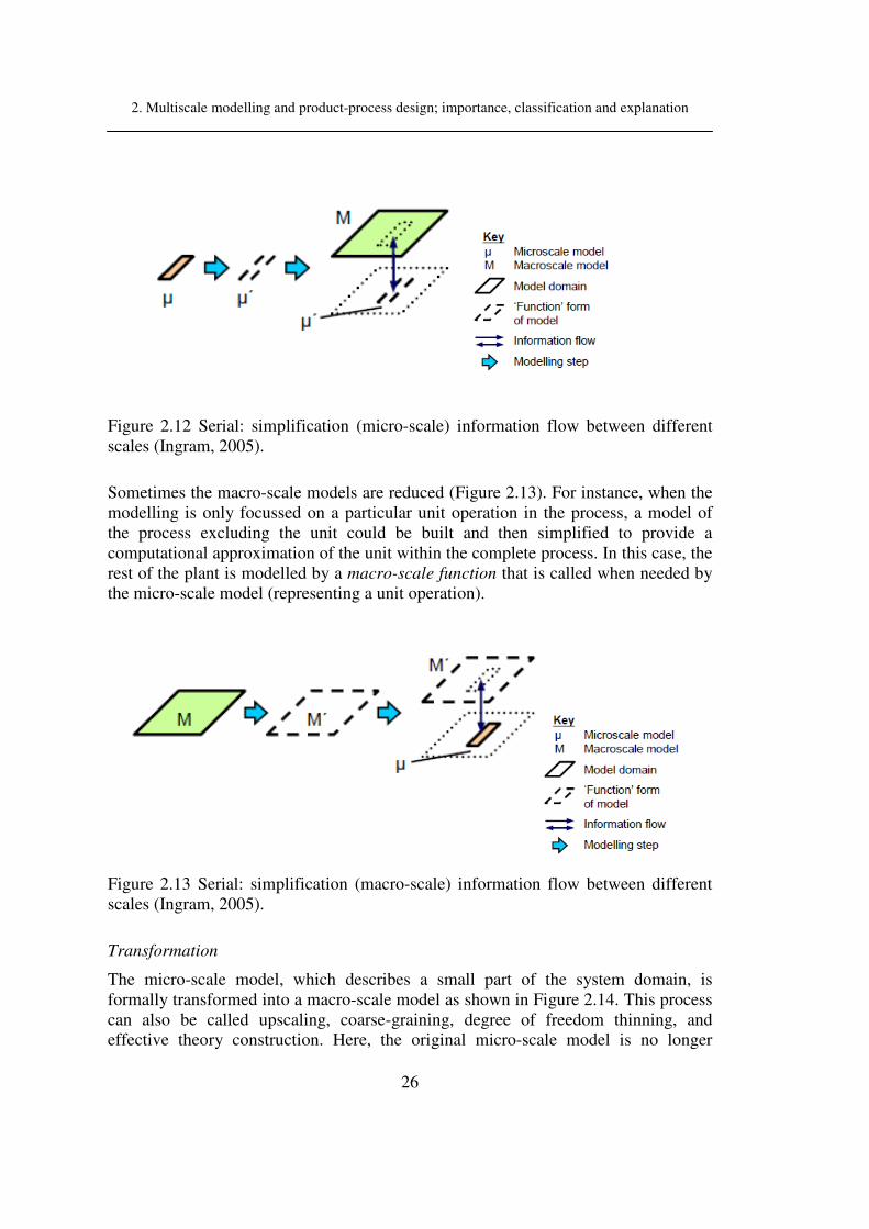
2. Multiscale modelling and product-process design; importance, classification and explanation
26
Figure 2.12 Serial: simplification (micro-scale) information flow between different scales (Ingram, 2005).
Sometimes the macro-scale models are reduced (Figure 2.13). For instance, when the modelling is only focussed on a particular unit operation in the process, a model of the process excluding the unit could be built and then simplified to provide a computational approximation of the unit within the complete process. In this case, the rest of the plant is modelled by a macro-scale function that is called when needed by the micro-scale model (representing a unit operation).
Figure 2.13 Serial: simplification (macro-scale) information flow between different scales (Ingram, 2005).
Transformation
The micro-scale model, which describes a small part of the system domain, is formally transformed into a macro-scale model as shown in Figure 2.14. This process can also be called upscaling, coarse-graining, degree of freedom thinning, and effective theory construction. Here, the original micro-scale model is no longer

2. Multiscale modelling and product-process design; importance, classification and explanation
27
needed and the system domain is described entirely by the new macro-scale model. Many techniques are used for upscaling: volume averaging, renormalisation and homogenisation, among others. No flow of information occurs between the micro-scale and macro-scale models during solution because the micro-scale model has been eliminated
Figure 2.14 Serial: transformation information flow between different scales (Ingram, 2005).
One way coupling
This option occurs when the nature of the system is such that information flows between the scales essentially in one direction only. Information may flow either from the micro-scale to the macro-scale (in Figure 2.15a), or vice versa (in Figure 2.15b). The independent model is solved first, then the dependent model is solved. The solution of the models is decoupled in one direction. An example, is the use of (micro-scale) molecular dynamics to calculate a diffusion coefficient, which is later used at the vessel (macro) scale via Fick’s law.
Figure 2.15 Serial: one-way information flow between different scales (Ingram, 2005).
(a) (b)
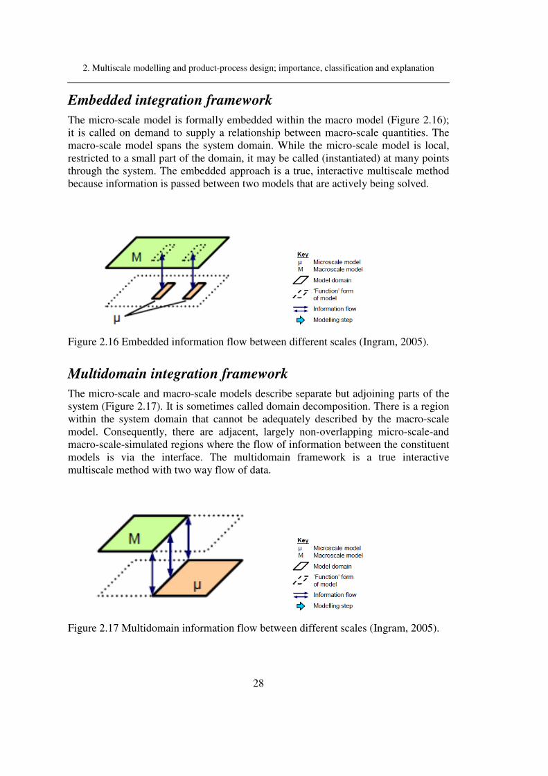
2. Multiscale modelling and product-process design; importance, classification and explanation
28
Embedded integration framework
The micro-scale model is formally embedded within the macro model (Figure 2.16); it is called on demand to supply a relationship between macro-scale quantities. The macro-scale model spans the system domain. While the micro-scale model is local, restricted to a small part of the domain, it may be called (instantiated) at many points through the system. The embedded approach is a true, interactive multiscale method because information is passed between two models that are actively being solved.
Figure 2.16 Embedded information flow between different scales (Ingram, 2005).
Multidomain integration framework
The micro-scale and macro-scale models describe separate but adjoining parts of the system (Figure 2.17). It is sometimes called domain decomposition. There is a region within the system domain that cannot be adequately described by the macro-scale model. Consequently, there are adjacent, largely non-overlapping micro-scale-and macro-scale-simulated regions where the flow of information between the constituent models is via the interface. The multidomain framework is a true interactive multiscale method with two way flow of data.
Figure 2.17 Multidomain information flow between different scales (Ingram, 2005).

2. Multiscale modelling and product-process design; importance, classification and explanation
29
Parallel integration framework
Both models span the system domain (Figure 2.18). The models may both have micro-scale and macro-scale features, however, they are complementary in the detail with which they describe the controlling phenomena. For this reason it is preferable to denote the component models as 1 and 2 in parallel integration. The few process engineering examples of this kind employ (i) a detailed hydrodynamic model with simple process kinetics operating in parallel with (ii) a detailed kinetic model that uses a simple flow pattern. The parallel models are usually iterated until convergence.
Figure 2.18 Parallel information flow between different scales (Ingram, 2005).
Based on Ingram’s (2005) proposals, a table (Table 2-1) that lists different integration framework strategies, has been developed. The table also lists the advantages, disadvantages and the potential application of each framework, with the aim of giving the model developer, useful information available in the literature on the process of interest.

2. Multiscale modelling and product-process design; importance, classification and explanation
30
Table 2-1 Advantages, disadvantages and application of the different integration frameworks (as proposed by Ingram, 2005).
Strategy Advantages Disadvantages Application
Simultaneously
High level of details
Flexibility
High accuracy
Very high computational burden.
Limited size of the system and length of time.
Used when: It is not possible to model any part of the system with sufficient accuracy at the macro level.
Serial
Potentially more efficient to the other four frameworks.
Enhanced calculation efficiency due to the use of powerful mathematical techniques for model reduction and analytical solution.
Sometimes have restricted accuracy.
Low flexibility in the approach.
Occasionally may need considerable effort to apply the mathematical techniques.
Simplification: when micro-scale (macro-scale) model can be simplified by order reduction or approximation techniques.
Transformation: Depends of the upscaling method chosen and the nature of the system, e.g. volume averaging, renormalisation, etc.
One way coupling: used when the nature of the system is such that one scale is dependent and the other is independent. No feedback between the scales.
Embedded
Natural appeal because of orderly.
Hierarchical nature.
Potential flexibility and accuracy of simultaneous integration.
Much lower computational load
Need to run the micro-scale model at all, because it may still consume the bulk of the computing resources.
When suitable macro-scale model exists but needs to be ‘informed’ by localised micro-scale information, and the micro-scale cannot acceptably be simplified. If a suitable simplification of the macro-scale model were available, serial integration via simplification should be used to reduce computing demand.
Multidomain
Couples micro-scale and macro-scale model to reduce the computational burden compared to simultaneous integration, maintaining micro-scale realism where needed.
Potential complexity of the micro-macro interface. It is important to guarantee the continuity of the thermodynamic properties and transport fluxes across the interface.
Used in problems where some parts of the system can be adequately described at the macro-level, while in other regions, only a micro-scale model will suffice. It is often used in model with heterogeneous media (e.g. gas and solid phases), and also applied for multidomain model in material science.
Parallel
A key benefit is the division of the system into two simpler problems becoming a little more systematic.
Inherent approximation of the method and its consequent limitations to systems with relatively weakly coupled mechanism
Suitable to be used when the time scale of the fluid flow is fast compared to other phenomena. Also used in some CFD/multizonal models for systems such as, bubble columns reactors, industrial crystallizers, etc.

3. Product-process design: A systematic modelling framework
31
3. Product-process design: A systematic
modelling framework
An efficient framework for product-process design is proposed, this framework allows the integration
of product-process design approaches (forward and reverse), multiscale models, computer-aided
modelling tools and a systematic work-flow and data-flow resulting in the development of a software
called, Virtual product-process design lab. This software allows the user to perform calculations
(virtual experiments) and design of products with the specific end-user properties required in the final
chemical product.
3.1. Systematic product-process modelling The development of a framework for performing modelling tasks in a systematic manner has been treated before, for instance, Hangos and Cameron (2001), Foss et al. (1998) and Marquardt (1996). Mathematical models that mimic the reality as near as possible are developed everyday. Mathematical modelling has been applied in different areas and fields, mainly related to the process and only recently there also has been focus on modelling for product design.
Sales-Cruz (2006) proposed a systematic modelling procedure consisting of the following ten steps:
(1) System description (model goal-set definition): The identification of an important starting point for all modelling exercises. This is usually a difficult task because of the difficulties associated with identifying the important system attributes defining the model objectives.
(2) Problem definition (model conceptualization and controlling factor identification): This step refines the process description from step 1 by adding the modelling goal, and fixes the degree of detail relevant to the modelling goal. For instance, when specifying the inputs and outputs for a, type of spatial distribution model (distributed (PDAE) or lumped (DAE)), the necessary range and accuracy of the model, and the time characteristics of the

3. Product-process design: A systematic modelling framework
32
process model (steady-state or dynamic) also need to be provided. According to Hangos and Cameron (2001), this step can be broken down into the following two tasks: (a) Identify the controlling factors; here, the physico-chemical phenomena that take place in the system must be identified. (b) Make assumptions; generally it is not possible to capture in a usable mathematical model all the factors influencing the problem that has been identified. The complexity of the problem can be simplified by reducing the number of factors under consideration, by neglecting some of the independent variables and by assuming relatively simple relationships.
(3) Model construction or selection: Once a problem has been defined, one must formulate it mathematically. Often the difficulty lies in the choice of complexity: one would like to employ a simpler model, but on the other hand one should include every relevant associated process occurring in the system needed to mimic the desired behaviour. The complexity of the model should depend on the final use of the model.
(4) Model analysis: Here, the equations representing the model are analyzed to identify and define a model solution strategy. In addition, model analysis is needed in the mathematical structure to ensure that the model is well posed (i.e. the degrees of freedom are satisfied); to avoid certain numerical problems such as high index; and, to break down a complicated model into simpler constituent processes (sub-models) which, for example, could operate on different space and time scales.
(5) Model data collection (need and source): In many modelling exercises, models are formulated using only first principles (white-box). However, mathematical models need often information (knowledge/data) to regress specific model parameters in order to match the desired system behaviour (grey-box model). If suitable measured data is not available, this situation may force the modeller to reconsider the decision in Steps 1 and 2, and therefore go back to change them.
(6) Model solution: Having a solution is just the beginning of the performance analysis of the model. It is possible to find obstacles in this step, for example, because the numerical computations cannot be established due to ill-posedness or stiffness of the equations. In some other cases the model may consist of mathematical equations or inequalities that must be solved, or require a best or optimal solution. Maybe one ends up with a model that it cannot be solved or interpreted. In such situations it is necessary to return to Step 2 and make additional simplifying assumptions, or sometimes to return to Step 1 to redefine the problem. The important issue here is the appropriate selection of the method of solution, matching the solution strategy and the mathematical structure of the model equations.
(7) Model verification: In this step the modeller needs to check whether the model is behaving correctly.

3. Product-process design: A systematic modelling framework
33
(8) Model validation: Before the model is released for general use, the calculated behaviour must be compared against the reality. Before designing validation tests and collecting data, there are several questions that should be asked: First, does the model answer the problem identified in Step 1? Second, can one really gather the data necessary to operate the model? Does the predicted curve fit the experimental data? Third, does the model make common sense? Usually, validation results indicate how to improve the model. For instance, one has to return to Step 1 and perform the step sequence again if the developed model is not suitable for the modelling goal; or one has to return to Step 2 and reformulate the assumptions if the model predictions are reasonable over a restricted range of the independent variables but very poor outside those values.
(9) Model implementation (model transfer): The model should be implemented such that it can be used for the purpose it was developed. Furthermore, unless the model is placed in a user-friendly form, it will quickly fall into disuse. Often the inclusion of an additional step to facilitate the collection and the input of data needed to solve the model determines its success or failure.
(10) Model documentation and maintenance: Model documentation is one of the key requirements for effective computer-aided modelling environments and probably one of the least developed. The most important issues are: (a) the systematic recording of all the underlying assumptions which are made during the course of the model development, (b) the documentation of the decisions or reasoning made to arrive at a particular model type, and (c) the generation of readable model descriptions and final reports for communication and archival purposes. Regarding model maintenance, it should be noted that the model is derived for the specific problem identified in Step 1 and from the assumptions made in Step 2. Therefore, if the original problem has changed in any way, then the model must be updated.
Comparing the above modelling steps with those proposed by Cussler and Moggridge (2002) for product design, it is possible to observe that both have similarities (although, more condensed for product design). In this direction, Gani (2005) pointed out that a successful development of model-based approaches will be able to reduce the time to market for one type of products, reduce the cost of production for another type of product, reduce the time and cost to evaluate yet another type of product. Here, the models to be used, need to be developed through a systematic data collection and analysis effort, before any model-based integrated product-process tools of wide application range can be developed. Finally, it should be noted that to find the magic chemical product, these computer aided model-based tools will need to be part of a multidisciplinary effort where experimental verification will have an important role and the computer-aided methods/tools could be used to design the experiments as well as to reduce the solution search space. Integration of product-process design through models and computer tools is a problem shown in Figure 3.1,

3. Product-process design: A systematic modelling framework
34
where the requirements for each of the steps/stages of the design, might or might not be assisted by information provided by experiment-based sources.
Figure 3.1 Models and tools in the integration of product-process design.
Gani et al. (2007) confirms that even though we do not have sufficient knowledge to understand all aspects of product-process design, do not have sufficient data to resolve all product-process design issues and/or do not have versatile models or a sufficient collection of models to cover a wide range of chemical products, it is still possible to solve many product-process design sub-problems correctly, consistently and efficiently, learning from past experiences so that the next time, solution of sub-problems requires smaller effort, using a product-process design framework, having as main parts: problem definition and the identification of candidates; performing of model-based simulations (or product-process behaviour); testing if the desired target (product) criteria have been matched; and finally, an evaluation step related to product quality and performance.
Based on the above discussion, the need for systematic methods and tools for innovative and fast solutions for a large number of products (in the market) and processes (to manufacture them) is important to recognize. The key to success in product-process design/development is first to identify the desired properties of a product and then to control product quality by controlling the structure, shape, odour, colour, etc, of the chemical in order to match the desired final products (Figure 3.2).
Experimental-based information

3. Product-process design: A systematic modelling framework
35
Another important criterion for development of many chemical products is to achieve “first time right” by establishing critical scientific and regulatory parameters early on and eliminating errors early in the design and development processes. Furthermore, there are chemical products where the reliability of the manufactured chemical product is more important than the cost of manufacture (such as, pharmaceuticals, drugs, etc.), while there are those where the cost of manufacture of the product is at least as important as the reliability of the product.
Figure 3.2 Variety of chemical products.
Thus, a multiscale product-centred process design framework is necessary and also is very important in order to achieve the needs mentioned above. This should combine modelling methods and tools able to manage mathematical models involving phenomena at different levels of abstraction in scales of time and length (multiscale modelling). This framework should consider the following characteristics:
• The first step should be defining a framework through which the development of the needed, methods and tools and their application of product-process design can be facilitated.
• Integration achieved by incorporating the stages/steps of the two (product &

3. Product-process design: A systematic modelling framework
36
process) design problems together into one integrated design process.
• The framework should be able to cover diverse product-process design problem formulations, be able to point out the needed stages/steps of the design process, identify the methods and tools needed for each stage/step of the design process and finally, provide efficient data storage and retrieval features and has multiscale modelling features.
• In an integrated system, documentation of the design, data storage and retrieval are very important because one of the objectives for integration is to avoid duplication of data generation and storage.
The design of the variety of products can be handled by a framework by plugging the necessary methods and tools into it. One of the principal objectives of the integration of product-process design is to enable the designer to make decisions and calculations that affect design issues related to the product as well as the process.
3.2. Multiscale modelling framework for
chemical product process design
The design, development and reliability of a chemical product and the process to manufacture it, need to be consistent with the end-use characteristics of the desired product. One of the common ways to match the desired product-process characteristics is through trial and error based experiments which can be expensive and time consuming. An alternative approach is the use of a systematic model-based framework according to an established work-flow in product-process design, replacing some of the time consuming and/or repetitive experimental steps. Furthermore, for many chemical products the appropriate models for product-process design need to have multiscale features as the properties defining the chemical structure and the product end-use characteristics are dependent on parameters of different size and time scales. The advantages of the use of the multiscale modelling approach in this case is that in the design, development and/or manufacturing of a product-process, the knowledge of the applied phenomena can be provided at diverse degrees of abstractions and details. Some authors (Charpentier, 2002; Cussler and Wei, 2003; Gani, 2004b; Voncken et. al., 2004; Charpentier, 2007 and Charpentier, 2005) have highlighted the importance of the multiscale and multidisciplinary approach in product-process design and identified design issues related to different scales of size, time and complexity.
In the development of the multiscale modelling framework for product-process

3. Product-process design: A systematic modelling framework
37
design, the work-flow and data-flow of information at the different steps of the product design, must include multidisciplinary and multiscale characteristics, and the gaps among the different disciplines/scales should be bridged. The product-process design modelling framework requires the interaction between human and computer, where the human is handling and controlling the work-flow, while the computer is carrying out the calculations in the work-flow and most of the tasks in the data-flow.
Therefore, a computer-aided framework for product-process design including a multiscale modelling option is very important for analysis, design, and/or identification of feasible chemical product candidates because it allows one to consider processing issues during the development of the product. The multiscale modelling framework should include the product and process design components, modelling tools and templates (work-flow) for guiding the user through the appropriate design steps. The integration of computational tools is also necessary to increase the application range of the computer-aided product-process framework; where the connection between computational tools could be established through well-defined COM-objects or the CAPE-OPEN standards.
3.2.1. Requirements in the multiscale modelling
framework for chemical product-process design
The multiscale modelling framework allows the user to cover a wide range of problems at different scales (of length and time) and disciplines of chemical engineering and science in an easy and efficient manner; achieving in this way the development of a product-process with the desired end-use characteristics. Another requirement of the modelling framework and the software architecture is a feature that provides the means for integration and merging of methods and tools from different sources. This architecture needs to accommodate models used for the prediction of the product behaviour/performance using modelling tools, which should provide interactions with modelling engines, external software through the use of COM-objects, and also with external simulators through the use of CAPE-OPEN standards (see Figure 3.12). Furthermore, to develop this multiscale modelling framework for chemical product-process design, a combination of different computational tools, such as, property prediction packages, modelling tools, simulation engines, solvent selection software, etc, are necessary together with a set of established systematic work-flows and data-flows for various types of design problems.
Figure 3.3 illustrates the flowdiagram of the multiscale modelling framework for chemical product-process design where 4 main parts can be found:

3. Product-process design: A systematic modelling framework
38
• problem definition,
• product design,
• product-process modelling,
• product-process evaluation.
Each part has sub-steps that guide the user through a systematic work-flow and data-flow to solve specific design problems.
Figure 3.3 Flowdiagram in the multiscale modelling framework in product-process design.
Problem definition
The multiscale modelling framework for chemical product-process design starts with the conceptual definition of the design problem (Figure 3.4), which concerns with setting the desired characteristics of the product, its properties, special qualities, ingredients to make the product, etc., that might apply for a new product or for existing products that need to be improved.
Figure 3.4 Problem definition section.

3. Product-process design: A systematic modelling framework
39
Product Design
Often, information needed to perform product behaviour analysis is lacking. To overcome these gaps of information, computer-aided methods and tools are employed. That is, the use of specialized computer-aided tools such as, databases containing properties of chemicals, property prediction packages, molecular and mixture design software, solvent selection tools, etc. are employed in order to address the issue of missing information.
In the product design part (as shown in Figure 3.5), the first sub-step involves generation of data/knowledge related to the product needs, ingredients, assumptions in the conceptual design work-flow, historical records, etc., that are needed in the subsequent steps and for future retrieval of information. Another sub-step in this part consists of the selection of the materials to be added to the product taking into consideration; its application, functional property values, primary property values, main active ingredients, solvents, coatings, etc., as well as the calculation of the necessary properties (such as, diffusion coefficients, partition coefficient, surface tension, etc.) related to the simulation model used in product performance evaluation.
Figure 3.5 Product design section.
Product-Process modelling
Once the necessary information for evaluating the product performance through the generated models has been retrieved, the product-process modelling section (illustrated in Figure 3.6) is using a modelling tool to assist in the simulation and generation of alternatives and verification of the formulated properties. The modelling tool should essentially be a software able to generate, analyze and simulate mathematical models without extra programming efforts. In this way, the predicted product behaviour is compared against the desired targets specified at the beginning,

3. Product-process design: A systematic modelling framework
40
and it is decided if the targets have been matched.
Figure 3.6 Product-Process modelling section.
If the design targets are not matched, a new product design problem (in the respective section illustrated with dashed line) is started, or, a model-based analysis is made and the subsequent steps repeated to find another solution. Another option is, once, the previous design has been performed, that a straight pathway to product-process modelling can be done, where some conditions regarding the product-process behaviour might be modified in order to verify the response of the performance, this part is illustrated by the dash-dot entering line between “perform product-process behaviour” and “product-process modelling tool” boxes. Another option is the model-based verification that basically consists of the sensitivity analysis to verify the parameters with most impact on the mathematical model output.
Product evaluation
If the targets are matched, before proceeding to manufacturing the product; an option to evaluate product-process performance must be conceptually performed (see Figure 3.7). Furthermore, an option to make sustainability analysis in order to evaluate the environmental and economical impact for the production and performance of the product should be provided.
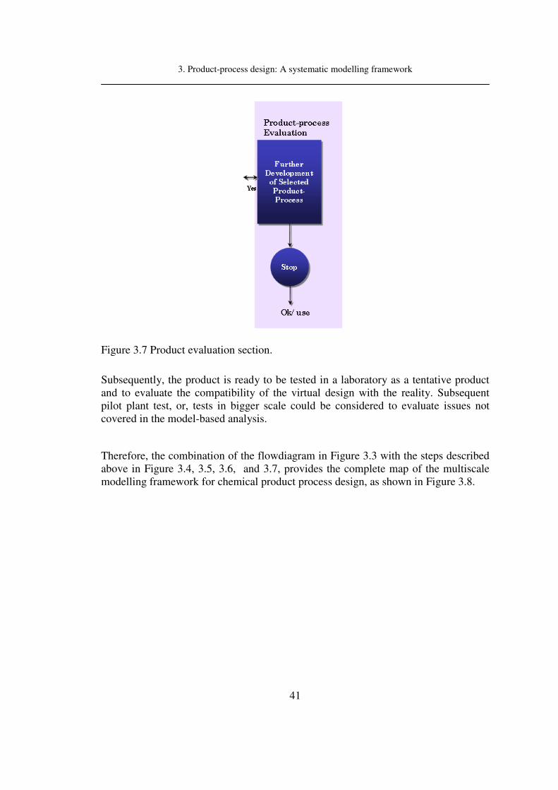
3. Product-process design: A systematic modelling framework
41
Figure 3.7 Product evaluation section.
Subsequently, the product is ready to be tested in a laboratory as a tentative product and to evaluate the compatibility of the virtual design with the reality. Subsequent pilot plant test, or, tests in bigger scale could be considered to evaluate issues not covered in the model-based analysis.
Therefore, the combination of the flowdiagram in Figure 3.3 with the steps described above in Figure 3.4, 3.5, 3.6, and 3.7, provides the complete map of the multiscale modelling framework for chemical product process design, as shown in Figure 3.8.

3. Product-process design: A systematic modelling framework
42
Fig
ure
3.8
Mu
ltis
cale
mo
del
lin
g f
ram
ewo
rk f
or
chem
ical
pro
du
ct-p
roce
ss d
esig
n

3. Product-process design: A systematic modelling framework
43
3.3. Different approaches in product design The importance of the needs for a framework in product-process design that allows the designer to consider different degrees of abstraction in size and time has been highlighted by Gani, (2004a) (2004b) (2005), Gani et al. (2007). However, the questions to be answer are, What is needed to develop the framework?. Which methods, algorithms and/or approaches would be employed to solve various design problems?. In this section, a general scheme of the algorithms, computational tools, etc., is presented together with their possible use in different work-flow and data-flow for diverse problems, in the product-process design.
3.3.1. Forward approach
Generally, model-based solution strategies are based on the brute force method (see Figure 3.9); where usually, input data (I) is necessary at the beginning of the solution of the problem in addition to the target criteria (Pt). Design properties (d) become fixed by the choice of a chemical(s) or materials that assist in the product manufacture or performance; it is necessary to use property models to estimate the properties ( θ (d)) that are needed to determine the process variables (X), which we
needed to predict the product/process behaviour (P(X)) of the design alternative, in order to compare it against the desired (target) Pt. If the target criteria have not been matched, the steps are repeated for another product-process design (d) until a match is obtained.
Figure 3.9 Model-based solution strategies based on brute force (forward approach) method.

3. Product-process design: A systematic modelling framework
44
3.3.2. Reverse approach
A novel methodology for product-process design using the reverse approach (see Figure 3.10) has been proposed by Eden et al. (2004) and was further extended by Soni (2008). It consists of a systematic framework for simultaneous solution of process/product design problems related to separation and material design (Soni, 2008). The methodology is based on the property clustering approach that allows one to perform design calculations on a component-free (or composition-free) basis. The approach consists in reformulating the conventional forward problem into two reverse problem formulations by decoupling the constitutive equations from the balance and constraint equations. The first reverse problem (stage I) is the reverse of a simulation problem. Here, the known target criteria (Pt(X)) are used to obtain (X) and then, knowing (I) and (X) and (Pt(X)), the ( θ (d)) are determined. In principle this part is
the reverse of a simulation problem. The second reverse problem (reverse property prediction, stage II) consist of given the values of the constitutive variables; determine the unknown intensive variables (d) (from the set of temperature, pressure and composition) and/or compound identity and/or molecular structure. As long as the targets are matched, the process model equations (minus the constitutive equations) do not need to be solved again. Similarly, solution of the molecular design problem to identify candidates that match the optimal design targets is the reverse of a property prediction problem (Harper et al., 1999).
Figure 3.10 Model-based solution strategies based on reverse approach method.

3. Product-process design: A systematic modelling framework
45
3.3.3. Adapting forward and reverse approaches to the
multiscale modelling framework for chemical
product-process design and computer tools to be
used.
The different approaches to solve a design problem have been presented above, but how can these different approaches be combined into a single multiscale modelling framework for chemical product-process design? This section presents the adaptation of the different approaches in order to present a data-flow and work-flow that will allow one to handle various types of product-process design problems.
Forward approach
The forward approach shown in Figure 3.9 can be adapted in the work-flow and data-flow of the multiscale modelling framework for chemical product-process design shown in Figure 3.8, as follows:
As shown in Figure 3.8, the chemical product-process design using the forward pathway starts with problem definition (I, Pt), desired properties, needs and quality of the product-process; documentation concerning the mathematical model of the product-process is given. In the next step, the selection of design properties (d) in terms of the selection of the material and the main ingredients of the product is made, together with the calculation of the necessary product properties (if necessary) using property models (< θ ). Once all, the necessary information/data is available, the next
step is to transfer the retrieved information to the product-process modelling (X) step. Here, the product behaviour and performance (P) using the modelling tools is predicted and tools that can assist in analysis, generation of alternatives and verification of the formulated product are employed. Subsequently, simulation results of product behaviour, are compared with the desired target (Pt) and if the target(s) has been matched, the next step is product verification through the use of more rigorous models and/or experiments can be performed. Furthermore, a sustainability analysis (if it is possible) might be carried out in order to study the environmental impact of the production of the product. If the target is not matched, one returns to one of the upstream steps to repeat the calculations. The important thing here to note is that for every choice of d, the calculation steps are repeated. Also, the evaluation of θ (d), for
which property models are needed, may make the resulting models very complex and even unsolvable.

3. Product-process design: A systematic modelling framework
46
Reverse approach
With respect to the application of the reverse approach (Figure 3.10) through the multiscale modelling framework for chemical product-process design (Figure 3.8), one starts with the definition of the product introducing input data (I) that basically is known information, together with the product targets (Pt). Given this information, the product-process modelling step (X) is carried out in order to calculate the constitutive variables ( θ ]) to match the product-process design targets and input data.
Consequently, results of the evaluation of the process model (consisting of thermodynamic properties, physical properties, etc.) are transferred to the property models section (d), to look for the product-process (material, molecular structure, process flowsheet, etc.) that could match the target property values of the constitutive variables. The search of the new product-process options can be sustained through the use of information found in the open literature; data bases specialized in the collection of product-process knowledge; use of group contribution methods to identify the materials that match the property targets (using molecular design tools, etc.). Once a match has been found, the product verification step is the same. If more than one match is found, the various alternatives are ordered according to performance criteria to find the best alternative.
3.4. Virtual product-process design Lab:
Applying the systematic
modelling framework
Usually, the solution of time consuming modelling tasks can be assisted by the use of computer-aided tools, allowing the user to perform the solution in an easier and faster manner, and thereby, also avoiding duplication of work. Implementation of the multiscale modelling framework for chemical product-process design (as shown in Figure 3.8) requires various items, such as, computer-aided tools, synthesis/design methods, work-flows and data-flows. All the methods and tools need to be integrated with the work-flow/data-flow for various product-process design scenarios. The result is a Virtual Product-Process Design Lab.
The Virtual Product-Process Design Lab (VPPD-l) is the name of the computer-aided tool developed in this PhD thesis (see Figure 3.11). This computer-aided tool incorporates a multiscale modelling framework for chemical product-process design. The main parts of the VPPD-l are: modelling data-flow and work-flow structure (section 3.2-3.3), model-based library (chapter 4), computer-aided tools (part in section 3.5) and synergy (section 3.4) between all the different entities.

3. Product-process design: A systematic modelling framework
47
Model-based library collection: the VPPD-l has a library of mathematical models applied to different type of phenomena in different problems (see models in chapter 4):
• Microcapsule-based controlled release of active ingredients (Controlled Release)
• Uptake of Pesticides
• Direct Methanol Fuel Cell (Fuel Cell)
Mathematical models in the model-based library can be used in the forward approach as well as in the reverse approach.
Work-flow and data-flow: work-flow and data-flow concerning different kinds of design approaches is also supported by the VPPD-l. They guide the user through the different steps of the multiscale modelling framework for product-process design (this part is illustrated in sections 3.2 and 3.3).
Computer-Aided tools: The use of some computational tools is important in the VPPD-l so that the user can perform calculations needed for the design or redesign of products. The following computer-aided tools have been included in the VPPD-l:
• CAMD (solvent selection, molecular and mixture design, Harper and Gani, 2000)
• ProPred (Property prediction of compounds, Marrero and Gani, 2001)
• DataBase Manager (huge database with information regarding to pure compound and different properties, Nielsen, et al., 2001),
• ICAS-MoT (model test-bed, to perform mathematical models; Sales-Cruz, 2006);
All of them are integrated in the ICAS software (Gani, et al., 1997). Moreover; the main menu of the VPPD-l has two links for two different external softwares. These external entities are connected using CAPE-OPEN standards, and an example of such a connection is highlighted in section 3.5.

3. Product-process design: A systematic modelling framework
48
Fig
ure
3.1
1 V
irtu
al P
rod
uct
-Pro
cess
Des
ign
Lab

3. Product-process design: A systematic modelling framework
49
3.5. Adding Models and expanding application
range: CAPE-OPEN standards
and multiscale modelling
Computer-aided design, analysis and/or operation of chemical products and processes that manufacture them require a number of computational tools. As these tools may come from different sources and disciplines, an important issue is how they can be used simultaneously and efficiently for the design, analysis and/or simulation of a specific process-product? One alternative is to employ CAPE-OPEN standard interfaces for integration of the set of diverse computational tools that may be needed to solve the problem. The objective of this chapter is to highlight, through examples, the integration of different computational tools according to problem specific work-flows/data-flows. The reliability of the integration of different tools is illustrated through two case studies. In case study 1, the tools Simulis® Thermodynamics (PME) and ICAS-MoT (PMC) are combined for the calculation of thermodynamic properties through the use of a standard middleware (DLL-file). In case study 2, the interoperability between the ProSimPlus simulator (PME) and ICAS-MoT (PMC) is highlighted for simulation of a new unit operation and combined with other unit operations that can be found in the host simulator. A ProSimPlus-ICAS-MoT – COFE interoperability is also carried out successfully to proof the interoperability of the different computational entities. Furthermore, the introduction of the multiscale modelling concept and its application through the CAPE-OPEN standards is highlighted.
3.5.1. What are CAPE-OPEN Standards?
The CAPE-OPEN effort is a standardisation process for achieving true plug and play of process industry simulation software components and environments, where, the CAPE-OPEN Laboratories Network (CO-LaN) consortium is in charge of managing the lifecycle of the CAPE-OPEN standard (Belaud and Pons, 2002). The objective of the CAPE-OPEN project was to clarify user priorities for process modelling software component/environment interoperability and promote the use of CAPE-OPEN standards to create commercially-valuable interoperability (Pons, 2005a).
The follow-up of the CAPE-OPEN project, called the Global CAPE-OPEN project, focused on the development of standards in new subfields of process modelling and simulation addressing complex physical properties, kinetic models, new numerical algorithms and distributed models. Also, future support for the development of
3. Product-process design: A systematic modelling framework
50
simulation software in the CAPE-OPEN-compliant interface components was established through the creation of the CO-LaN. The CO-LaN promotes the integration of open process simulation technology in the work process, and use of CAPE-OPEN compliant interoperated software for taking real industrial case studies and in assessing the use of CAPE-OPEN technology. In addition, CO-LaN provides support and user training; definition of open standards for new technologies beyond process modelling and simulation, developing prototypes for on-line systems, discrete and mixed batch-continuous processes, finer granularity interfaces, and scheduling and planning systems (Braunschweig et al., 2000).
Currently, several commercial simulator vendors, modelling tools developers, etc. have incorporated CAPE-OPEN standard in their products, allowing the user a better and easier manner for implementation/combination among process modelling components (PMC) and process modelling environments (PME) (Pons, 2003).
CAPE-OPEN is an abstract specification that can be subsequently implemented in COM, CORBA and .NET for bridging PMCs and PMEs. Recently, the .NET framework has been introduced as a new alternative to provide the interoperability among different platforms. This new technology has been presented by Microsoft and it seems to be visualized as the future of the connections between different platforms. CO-LaN has published guidelines on how to use .NET with CAPE-OPEN, this is available in the CO-LaN website at http://www.colan.org/News/Y06/news-0616.htm.
3.5.2. Interoperability between ICAS-MoT and Process
Simulators (ProSimPlus and Simulis
Thermodynamics)
The process modelling component (represented by ICAS-MoT) is able to achieve interoperability and be wrapped for use within a PME (represented by a simulation engine, external software and external simulator) through CAPE-OPEN interfaces. Figure 3.12 illustrates the interaction that can be done between a PMC and a PME. This interaction has been applied in this chapter for two case studies. In both cases, the ICAS-MoT is representing a PMC with different models. In the first case, the PMC is integrated with a PME (represented by Simulis® Thermodynamics) while in the second case, the PMC is integrated with a PME (represented by one external simulator as ProSimPlus). To establish the integration, here, the following components are needed:
• PME (Process Modelling Environment)

3. Product-process design: A systematic modelling framework
51
• PMC (Process Modelling Component)
• Middleware (COM)
Figure 3.12 Interoperability between the PMC and PME.
Process Modelling Component (PMC)
Process modelling components are objects that can be added to the flowsheet to represent unit operations or mathematical/information/energy flows within the flowsheet, thermodynamic property models, reaction models or mathematical model solvers (Barrett and Yang, 2005). PMCs are pieces of software that are defined for a specific function. Most of the applications are for: physical properties, unit operation modules, numerical solver and flowsheet analysis tools. This work focuses mostly on the connection of PMCs related to physical properties and unit operation to an appropriate PME.
As far as physical properties are concerned, they are an important part in the evaluation of chemical processes that involve some kind of phase equilibrium calculations (vapour-liquid, liquid-liquid, solid-liquid and so on) or some transport properties or the use of some derivatives of some properties with respect to temperature or pressure (i.e.; fugacity coefficients, enthalpy, etc.) using some equations of state or special correlations (depending on the property that it is being calculated) that can not be easily found in some commercial or free software.
In CAPE-OPEN compliant PMCs for unit operations, the interface includes ports that can be classified as material, energy and information ports. In this work, the notion of Material Object is used to represent a material stream. In fact, a CAPE-OPEN Material Object is a container of properties describing the material stream. Also, this object allows property and equilibrium calculations by its associated CAPE-OPEN Thermo Property Package. This association is performed by the simulator (PME).

3. Product-process design: A systematic modelling framework
52
The CAPE-OPEN Material Object can also provide pure component properties, constant or temperature dependent. CAPE-OPEN Material Objects are connected to the Unit Operation using inlet or outlet material ports. It is not necessary to connect all ports but, in many cases, a minimum number of connections (inlet and outlet) must be respected. Parameters are another important part in CAPE-OPEN. They can be classified into private and public parameters. On the one hand, private parameters are only modifiable from the Unit Operation itself using, in general, a graphical user interface. On the other hand, we find public parameters, also called CAPE-OPEN parameters, which are exposed to the outside of the Unit Operation. Private and public parameters can be input or output parameters of the model. In some cases, the values of these parameters can be imported or exported using CAPE-OPEN Information Objects connected to information ports. Figure 3.13 is showing a scheme of a CAPE-OPEN Unit Operation. Some PMCs that can be found are: ICAS-MoT, Aspen Properties, ChemSep, CPA Property Package and so on.
Figure 3.13 CAPE-OPEN Unit operation.
Process Modelling Environment (PME)
The process modelling environment supports the construction of process models from first-principles and/or library of unit operation models, number of model-based applications as, simulation, optimization, and they may use of one or more PMCs (Pons, 2005b); furthermore, PMEs allow process engineers to use software from heterogeneous sources operating together to carry out complex model-based tasks

3. Product-process design: A systematic modelling framework
53
(Braunschweig et al., 2000). PMEs also consist of the graphical interface and functionality required to create the flow network being modelled; input, review and modify values for parameters of components; input, review and modify material or energy flows, and calculate the conditions of the flowsheet based on the inputs (Barrett and Yang, 2005). Some examples of PMEs that can be found are: ProSimPlus, Simulis® Thermodynamics, Aspen Plus, COFE, gPROMS and so on.
Middleware
One of the most important parts to carry out this interoperability between the PMCs and PMEs is the part that allows connecting those entities. CAPE-OPEN has chosen to adopt a component software and object-oriented approach that views each PMC as a separate object. All communication between objects is handled by “middleware” such as CORBA or COM (Braunschweig et al., 2000) and now already the .NET framework. Figure 3.14 is illustrating the three main components to carry out the combination of software components through CAPE-OPEN standards.
Figure 3.14 CAPE -OPEN Components
PMC offers a “CAPE-OPEN Plug” when it can be used within different PMEs using CAPE-OPEN interfaces. CAPE-OPEN Unit Operations offers a CAPE-OPEN Unit Plug, while, CAPE-OPEN Thermo Property Packages offers a CAPE-OPEN Thermo Plug. For PMEs, the “socket” term will be used to express the capacity to employ
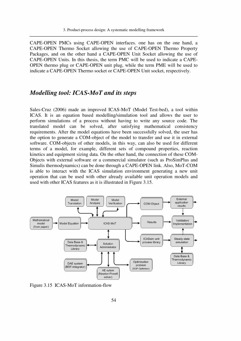
3. Product-process design: A systematic modelling framework
54
CAPE-OPEN PMCs using CAPE-OPEN interfaces. one has on the one hand, a CAPE-OPEN Thermo Socket allowing the use of CAPE-OPEN Thermo Property Packages, and on the other hand a CAPE-OPEN Unit Socket allowing the use of CAPE-OPEN Units. In this thesis, the term PMC will be used to indicate a CAPE-OPEN thermo plug or CAPE-OPEN unit plug, while the term PME will be used to indicate a CAPE-OPEN Thermo socket or CAPE-OPEN Unit socket, respectively.
Modelling tool: ICAS-MoT and its steps
Sales-Cruz (2006) made an improved ICAS-MoT (Model Test-bed), a tool within ICAS. It is an equation based modelling/simulation tool and allows the user to perform simulations of a process without having to write any source code. The translated model can be solved, after satisfying mathematical consistency requirements. After the model equations have been successfully solved, the user has the option to generate a COM-object of the model to transfer and use it in external software. COM-objects of other models, in this way, can also be used for different terms of a model, for example, different sets of compound properties, reaction kinetics and equipment sizing data. On the other hand, the connection of these COM-Objects with external software or a commercial simulator (such as ProSimPlus and Simulis thermodynamics) can be done through a CAPE-OPEN link. Also, MoT-COM is able to interact with the ICAS simulation environment generating a new unit operation that can be used with other already available unit operation models and used with other ICAS features as it is illustrated in Figure 3.15.
Figure 3.15 ICAS-MoT information-flow

3. Product-process design: A systematic modelling framework
55
The flow of information among the different modules is shown in Figure 3.15, where the main features of the modelling tool are:
• Model equation
• Model translation
• Model analysis
• Model verification
• Model solution
• Exporting models
• Model validation
A description of the different parts is provided below.
Model Equation
Model equation (Figure 3.16) is introduced through the use of one graphical user interface that provides interaction between the modeller and the modelling tool, where the editor serves to define the problem. The flow of data is controlled from here.
Figure 3.16 ICAS-MoT : Model equation.
An example of a simple ICAS-MoT code is also shown in Figure 3.16. The ICAS-
#Modelling of Unsteady state free settling in Stokes Law regions
#Mass of spherical particle
mass=(3.1415/6)*diapar^3*denpar
#Weight of spherical particle
w=(3.1415/6)*diapar^3*denpar*grav
#Buoyancy force
Fb=(3.1415/6)*diapar^3*denflu*grav
#Partical Reynolds number
Re=(denflu*U*diapar)/visflu
#Stokes law drag coefficient
Cd=24.0/Re
#Drag force
Fd=(3.1415/8)*diapar^2*denflu*U^2*Cd
#Unsteady state conditions a momentum balance on the particle
dU=(1/mass)*(w-Fb-Fd)

3. Product-process design: A systematic modelling framework
56
MoT language was developed in such a way that the user only is required to introduce information (mathematical equations) almost in the same manner as the user is visualizing the source (publications, literature, etc.). The structure of the code follows some simple rules suitable to be used for people involved in the engineering and mathematical fields.
Model translation
The model equations collected from the GUI have to pass through a syntactic and lexical recognition. The model translation process (Figure 3.17) starts by reading the input line equation and parsing it, that is, breaking the equations into elementary components through which the line equation (source code) is transformed to the translated code (object) step by step. The process starts scanning the text-base to ensure mathematical consistency. After the variables have been validated, each equation and variable is expanded to match the current size of the problem, usually depending of the number of compounds present in the system. Once, the equations have been expanded, giving the actual equations to be solved, the variable classification step is invoked. The variables are classified as RHS (right hand side of the equation) and LHS (left hand side of the equation); RHS contents different kind of variables such as, dependent, dependent prime, parameter, known and unknown; with respect to LHS, variables are classified as explicit type. Afterwards, the model is ready to be solved.
Figure 3.17 ICAS-MoT : Model translation.

3. Product-process design: A systematic modelling framework
57
The translated equations must be stored. Any expression recognized as a valid expression is passed to the model translator engine for analysis.
Model Analysis
The model analysis (Figure 3.18) starts with the manipulation of the model equations so that they are transformed into a consistent set of equations that can be solved in a robust and efficient manner. Model analysis involves:
• Degree of freedom (DOF) analysis
• Determination of the structure of the equation system
• Index analysis
• Partitioning and ordering of the model equations
• Determination of the sparse pattern
• Analysing for numerical ill-condition expressions
• Analysing for stiffness of differential equations.
Figure 3.18 ICAS-MoT : Model analysis.
Model Verification
This part of the software (see Figure 3.19) checks if the equations have some terms where it can be possible to find divisions by zero or can be sending a warning alert to check if the numerical values have been introduced correctly in the equations.

3. Product-process design: A systematic modelling framework
58
Figure 3.19 ICAS-MoT : Model verification.
Model Solution
The data-flow in the input is in the form of equations. In the return, the variables (unknowns) come back with values obtained after the solution of the model (Figure 3.20).
Figure 3.20 ICAS-MoT : Model solution.
The model solution checks if the equations are ordered. After that, the equations are solved and the variables are updated, and the administrator verifies that the required information is present in terms of the solution. The information exchanges between the variable update and the solver library can be carried out several times. The solver
AE
ODE
PDAE
( )x
( ) 0
( , ) 0
( , , ) 0
=
=
∂=
∂
x
x
x
f
f t
xf t
r
( )x

3. Product-process design: A systematic modelling framework
59
library receives equations and it returns a set of variables with values after the model equation is solved.
Exporting and Importing Models
An interface needs to be designed to help the CAMS users work with other application environments. This interface has to support access to dynamic link libraries (DLLs) and servers based upon Component Object Model (COM).
Figure 3.21 ICAS-MoT: Exporting model.
The exporting of models can de done in two ways (Figure 3.21):
• COM-Objects: This consists of reusable pieces of code and data in binary form that can be plugged in to other software components from other vendors with relatively little effort.
• The set of equations can be exported to the Icassim unit. The model developed in the ICAS-Mot environment is allocated a new unit in the icassim module, thus allowing the user to perform a simulation in the ICAS simulation environment.
ICAS-MoT is also able to import mathematical models in native text file format (Equation file) or XML-files format (Extensible Markup Language). The advantage is that the files might be created in a proper editor program, and subsequently, the model contained in the file is pre-screened and pre-translated to make sure that is valid and ready to be solved in ICAS-MoT.
0101101
0010011
101110

3. Product-process design: A systematic modelling framework
60
Model Validation
An important part of the mathematical modelling cycle is validation of the proposed model. Various statistical tests and residual analysis tools are available including marginal and simultaneous tests for parameter significance and correlation analysis of residuals computed from validation data sets, i.e. data sets that were not used for parameter estimation.
3.5.3. Case Studies: Operation of PMCs and PMEs;
illustrated examples.
Simulis® Thermodynamics – ICAS-MoT Interaction.
The first case study is demonstrating the integration between ICAS-MoT and Simulis® Thermodynamics (see Figure 3.22), which is carried out through the use of a DLL file as the middleware, where Figure 3.22 is illustrating the general structure of the combination of these different computational tools. The introduction of data is carried out through Simulis® Thermodynamics that provides a graphic interface for this purpose. Information (data) is transferred through the DLL file where variables that are shared between the integrated computational tools are specified. This information is transferred to ICAS-MoT to carry out the calculations using the ICAS-MoT solver. Afterwards, results are retuned through the DLL file again and presented in the Simulis® Thermodynamics dialogs in the same way as calculations carried out using its native models. This case study is illustrated using the calculation of fugacity and activity coefficients where the mathematical (thermodynamic property) model is specified in the ICAS-MoT file.

3. Product-process design: A systematic modelling framework
61
Figure 3.22 ICAS-MoT Interoperability with Simulis® Thermodynamics.
Fugacity and Activity Coefficients Calculation.
In order to show the reliability of this integration, calculations of fugacity coefficients have been performed with three different mathematical model equations of state: SRK, SAFT and PC-SAFT. Note that the same middleware has been used for the different equation of state models (see Figure 3.23). For instance, whether one wants to perform the calculations using the SAFT model and afterwards with the PC-SAFT model, the only “work” needed is to change the ICAS-MoT file and it would be possible to perform the calculations in Simulis® Thermodynamics without any extra effort. The data-flow taking place through the DLL file involves the following variables: temperature (T), pressure (P), vapour composition (Yv) and fugacity coefficients in vapour phase (Phiv). Among these variables, (T, P and Yv) are specified in Simulis® Thermodynamics and through the DLL file to ICAS-MoT, which then employs the specified model to calculate the fugacity coefficients (PhiV) send the information to Simulis® Thermodynamics through the DLL file.
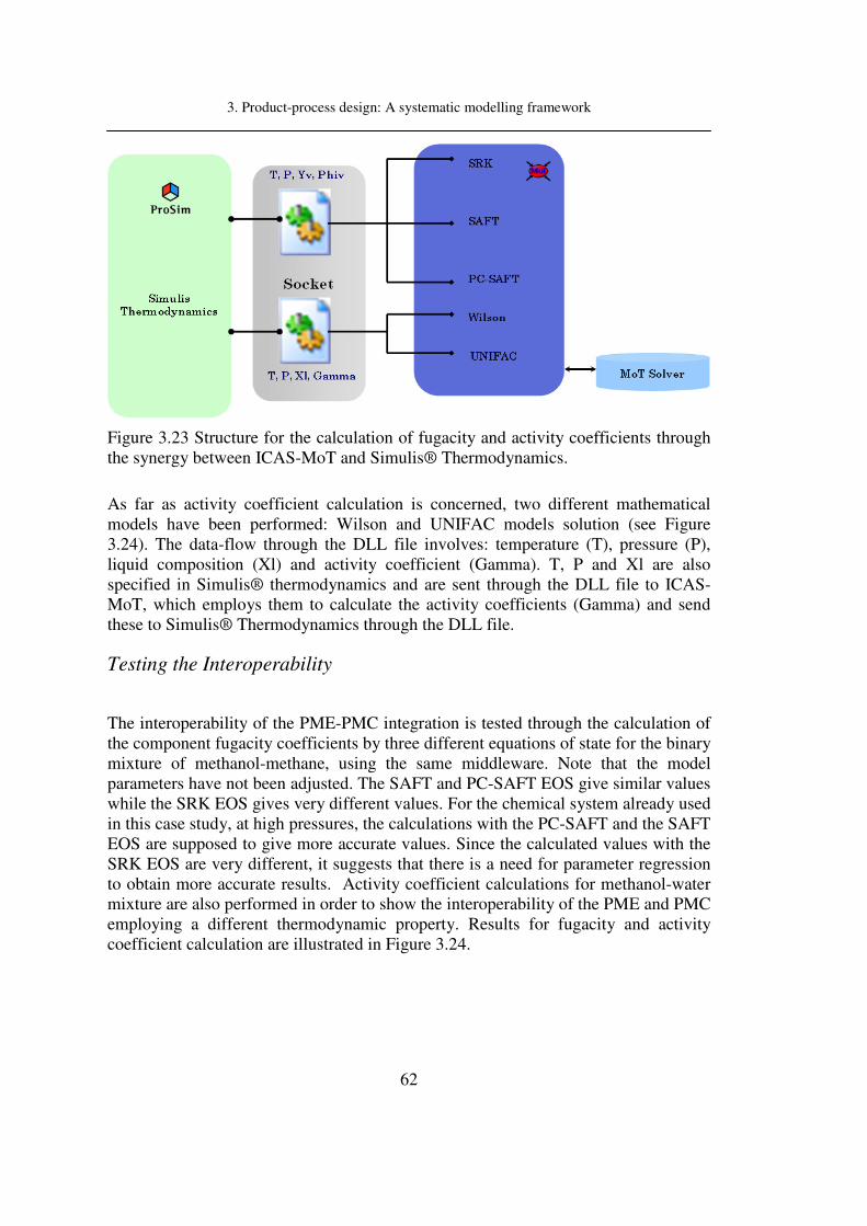
3. Product-process design: A systematic modelling framework
62
Figure 3.23 Structure for the calculation of fugacity and activity coefficients through the synergy between ICAS-MoT and Simulis® Thermodynamics.
As far as activity coefficient calculation is concerned, two different mathematical models have been performed: Wilson and UNIFAC models solution (see Figure 3.24). The data-flow through the DLL file involves: temperature (T), pressure (P), liquid composition (Xl) and activity coefficient (Gamma). T, P and Xl are also specified in Simulis® thermodynamics and are sent through the DLL file to ICAS-MoT, which employs them to calculate the activity coefficients (Gamma) and send these to Simulis® Thermodynamics through the DLL file.
Testing the Interoperability
The interoperability of the PME-PMC integration is tested through the calculation of the component fugacity coefficients by three different equations of state for the binary mixture of methanol-methane, using the same middleware. Note that the model parameters have not been adjusted. The SAFT and PC-SAFT EOS give similar values while the SRK EOS gives very different values. For the chemical system already used in this case study, at high pressures, the calculations with the PC-SAFT and the SAFT EOS are supposed to give more accurate values. Since the calculated values with the SRK EOS are very different, it suggests that there is a need for parameter regression to obtain more accurate results. Activity coefficient calculations for methanol-water mixture are also performed in order to show the interoperability of the PME and PMC employing a different thermodynamic property. Results for fugacity and activity coefficient calculation are illustrated in Figure 3.24.

3. Product-process design: A systematic modelling framework
63
Figure 3.24 Results for fugacity and activity Calculations using ICAS-MoT and Simulis® Thermodynamics.
ProSimPlus – ICAS-MoT Interaction
The interoperability between ProSimPlus and ICAS-MoT is shown in this case study. A new unit operation (Direct Methanol Fuel Cell) model employing a multiscale modelling approach is combined with unit operations that can be found in the model library of ProSimPlus; other examples of this interoperability between ProSimPlus and MoT can also be found in Morales-Rodriguez et al. (2006). The first step is to understand the interoperability between the PMC and PME.
Figure 3.25 illustrates a “Generic CAPE-OPEN Unit Operation” where objects are wrapped by an ICAS-MoT object (COM object) representing a model generated
0 5 10 15 20 25 30 35 40
0.970
0.975
0.980
0.985
0.990
0.995
1.000
1.005
1.010
1.015
Methane Fugacity Coefficient
ΦΦ ΦΦ (
Fu
ga
cit
y C
oe
ffic
ien
t)
Pressure, atm
SRK
SAFT
PCSAFT
0 5 10 15 20 25 30 35 40
0.75
0.80
0.85
0.90
0.95
1.00
Methanol Fugacity CoefficientΦΦ ΦΦ
(F
ug
ac
ity
Co
eff
icie
nt)
Pressure, atm
SRK
SAFT
PCSAFT
0.8 0.9 1.0 1.1 1.2 1.31.0
1.1
1.2
1.3
1.4
1.5
1.6
1.7
Methanol Activity Coefficient
γγ γγ (A
cti
vit
y C
oeff
icie
nt)
Pressure, atm
Wilson
UNIFAC
0.8 0.9 1.0 1.1 1.2 1.31.00
1.05
1.10
1.15
1.20
1.25
Water Activity Coefficient
γγ γγ (A
cti
vit
y C
oeff
icie
nt)
Pressure, atm
Wilson
UNIFAC

3. Product-process design: A systematic modelling framework
64
through ICAS-MoT (an ICAS-MoT file) and where all the necessary interfaces for connection to other tools are CAPE-OPEN compliant. An XML configuration file describes the mapping between variables of the ICAS-MoT model and variables required by CAPE-OPEN specifications.
Figure 3.25 ICAS-MoT CAPE-OPEN Unit Operation.
The input Material Objects must, at least, provide the following variables: temperature, pressure, composition (either total flowrate and molar fractions, either partial flowrates) through the COM interfaces. More generally, the wrapper will provide/ask to MoT Objects for each property described in the XML configuration file (containing the mapping between ICAS-MoT Objects variable and wrapper variables). The values of the variables are obtained using the ICAS-MoT model and calculated by the ICAS-MoT Solver. As far as output Material Objects concerns, the same variables should be described and returned plus the enthalpy of the stream (in this case calculated by ProSimPlus).
The generic CAPE-OPEN MoT Unit Operation uses configuration files to determine the number and the definition of ports, variables and constants. These files are text files (“.MoTUO” filename extension) with a specific syntax and can be written with any text editor. They are based on the well known XML and XSD standard. The
3. Product-process design: A systematic modelling framework
65
structure of the XML configuration file consists of three main sections: “Globals”, “UserParameters” and “MaterialPorts” as shown in Figure 3.26. First of all, the encoding type used in the XML file (in our case "ISO-8859-1") and the schema used in the XML file are specified. The schema describes the grammar of the XML file. The “Globals” block consists of general information about: the unit operation, minimum and maximum number of material ports, compounds, etc. The “UserParameters” block describes the values of parameters that the user can modify through the GUI (Graphical User Interface) of the unit operation in the simulator. Here, it is possible to specify the type of parameter, the default initial value, the lower and upper bound for the parameters and so on. The “MaterialPorts” block consists of a list of ports. These ports describe the connections available for the simulator and the values to copy from/to CAPE-OPEN Material objects connected to the port. Each “MaterialPort” section describes the connection port, variables and constants used to communicate with the CAPE-OPEN Material Objects connected to these ports. The “MaterialPorts” block also contains the “variables” sections where the list of variables is specified. These variables are used to transfer data from and to the CAPE-OPEN Material Objects connected to the port and are non constant properties of the mixture or of a pure compound. Note that since the XML configuration file specifies and controls the information shared between the PMC and PME, its construction needs to be done carefully.

3. Product-process design: A systematic modelling framework
66
Figure 3.26 XML configuration file structure.
A direct methanol fuel cell mathematical model described in Table 4-5 (section 4.2),

3. Product-process design: A systematic modelling framework
67
is employed in this integration between ICAS–MoT and ProSimPlus 2. The different parts of the mathematical model are assembled through the middleware (CAPE-OPEN interface) within the PME (external simulator) as shown in Figure 3.27. The construction of the flowsheet is carried out by adding the corresponding identifiers of the unit operation(s) as well as the feed, product and connection streams, available in the process flow diagram menu on the left side of the graphic user interface window. Once, the addition of the unit operation has been done, a dialog box window appears to introduce the information, conditions and values for each unit operation that have been chosen previously. It is convenient to highlight that the information introduced in the dialog box window for the generic CAPE-OPEN unit operation (in the PME) corresponds to the parameters specified in the XML configuration file in the “UserParameters” block.
Figure 3.27 Flowsheet in the ProSimPlus simulator including the CAPE-OPEN unit operation using an ICAS-MoT model.
The flowsheet shown in Figure 3.27 illustrates a small part of the industrial production of methanol where this product is generated in the reactor by chemical reaction between carbon dioxide and hydrogen. The outlet flowstream of the reactor is composed of methanol, water (as the reaction products) and the reactants. This

3. Product-process design: A systematic modelling framework
68
mixture is fed to a unit operation representing a membrane unit operation where pure methanol is obtained at the top and the mixture of the four compounds is withdrawn at the bottom. The top product is feed in the Generic CAPE-OPEN unit operation that is representing a DMFC unit operation and its mathematical model is generated and represented by an ICAS-MoT file. Both scenarios mentioned below are described in separate ICAS-MOT files but work with the same XLM file, thereby providing a “plug and play” option.
Dynamic simulation results for the flowsheet presented in Figure 3.27 are shown in Figure 3.28. Note that the PME simulator is not a dynamic simulator but the Direct Methanol Fuel Cell model contained in the ICAS-MoT file is. The simulation strategy involved was changing the final time of integration of the model directly in ICAS-MoT. This was done in order to see the different results that can be obtained for the dynamic simulation, with or without the multiscale feature. Obviously, the two models should give the same steady state values but the path to achieve them would be predicted differently.
Methanol bulk composition and carbon dioxide bulk concentration, which are variables at the meso-scale level were chosen to illustrate the different results obtained for each scenario. Figure 3.28 (a) is showing the bulk composition of methanol present in the fuel cell obtained with the multiscale (MS) and Single-scale (SS) models. As it can be seen, the values of these variables at the steady state are quite similar, but they are not for the transient state where some differences in the composition along time can be noted. Those details are the extra information that can be obtained through the use of the multiscale modelling approach. The bulk compositions for carbon dioxide are also shown in Figure 3.28 (b) using the multiscale and single-multiscale models. The simulated results are also different for the two modelling approaches. Certainly, it is possible to add further details of the phenomena that are occurring in the process depending on whether the model for lower or higher scale are available or necessary for the study. The multiscale modelling framework is useful for the integration, connection and description at different scales, but the mathematical model to use will depend on the scenario and objectives of the model-based study.

3. Product-process design: A systematic modelling framework
69
0 500 1000 1500 2000 2500 3000 3500 40000.0000416
0.0000417
0.0000418
0.0000419
0.0000420
0.0000421
0.0000422
0.0000423
0.0000424
0.0000425
0.0000426
0.0000427
0.0000428
0.0000429
CC
H3O
H , m
ol/
m3
Time, s
SS
MS
0 500 1000 1500 2000 2500 3000 3500 40000.00E+000
5.00E-008
1.00E-007
1.50E-007
2.00E-007
CC
O2
, m
ol/
m3
Time, s
SS
MS
Figure 3.28 Results of the CAPE-OPEN unit operation embedding multiscale modelling.
ProSimPlus – ICAS-Mot – COFE Interaction
A combination between the Generic CAPE-OPEN Unit Operation and COFE (taken from www.cocosimulator.org) has also been tested in order to prove the interoperability issues with another PME different than ProSimPlus. A simple splitter
(a)
(b)

3. Product-process design: A systematic modelling framework
70
mathematical model is used in this interoperability test. Figure 3.29 is showing the different windows when ProSimPlus-ICAS-MoT – COFE based calculations are carried out: (a) is showing the COFE interface with the generic CAPE-OPEN unit operation that is using an ICAS-MoT model, while, (b) it is showing the window with the outstream results of the CAPE-OPEN unit operation, and these confirm the possibility of the interoperability between these computational tools.
Figure 3.29 ProSimPlus - ICAS-MoT - COFE interoperability.
Note that the use of the CAPE-OPEN standards facilitates the simulation of new unit operations in PMEs or those that cannot be found in commercial simulators. The use of the multiscale modelling approach embedded in the model of the new unit operation is used to highlight the importance of selecting the appropriate details of the model needed to match the objective.

3. Product-process design: A systematic modelling framework
71
3.5.4. Importance of multiscale modelling in the
integration of the modelling tools and external
simulators and software.
The advantages of the use of CAPE-OPEN standards for the integration of different tools (computer-aided modelling tools, process simulators, property prediction packages, etc.) have been tested and highlighted in this chapter. Furthermore, the use of a multiscale modelling approach in the simulation of unit operations not found in the host PME has been highlighted for different scales and objectives of the model, showing the advantages of the synergy of CAPE-OPEN standards and multiscale modelling approach.
Among the main entities used in the combination of different computational tools applied with the aim of application in chemical engineering, the middleware is one of the key parts that allows the combination of those different units; in the applications presented in this chapter, a standard middleware for thermo-models interoperability aspects of the integrated tools, has been illustrated with the scope of performing the calculations of fugacity coefficients and activity coefficients by different property models.
On the other hand, the integration between ICAS-MoT and ProSimPlus for reliable simulation of any unit operation is also shown, where models can be supplied from different sources being easily achieved through plug & play (interoperability) of software tools and models. Here, the CAPE-OPEN interface for unit operations plays an important role in order to perform the simulation.


4. Multiscale model-based library: development and testing
73
4. Multiscale model-based library:
development and testing
Three different examples (case studies) involving multiscale modelling data-flow between the different
scales are illustrated in this chapter. These case studies highlight the use of models for: batch catalytic
fluidized bed reactor, direct methanol fuel cell and microcapsule controlled release of active
ingredients.
4.1. Fluidized bed reactor Fluidized bed reactors have played a major role in the development and manufacture of different products in the chemical industry. Fluidized bed reactor have been used for, coal combustion, gasification and liquefaction, solid residue pyrolysis, production of polymers, catalytic fuel and waste combustion, reforming of acetic acid, naphtha as well as natural gas. One of the first commercial fluidized bed reactors was introduced in USA in 1942; it was applied in the petroleum industry and consisted of a fluid catalytic cracker (FCC) unit created for use by Standard Oil Company’s refinery. In the subsequent years the number of FCC units increased due to the need for combustibles during World War II. Afterwards, the use of gasoline as a fuel in automobiles and the use of FCC for the production of the combustible triggered even more the construction and use of fluidized bed reactors. Catalytic combustion is also employed in waste combustion, which is generally used in the domestic and industrial heat sources, such as, radiant heaters, stoves with catalytic burners, boilers and gas turbines in the power plant industry (Ismagilov & Kerzhentev, 1999). As far as reforming of natural gas is concerned, fluidized bed reactors are used for the production of hydrogen utilized by many processes, such as, oil refining, methanol production, metallurgy, ammonia production, space transportation, etc.
The advantages of the use of these fluidized bed reactors are, for instance: the uniform temperature gradient in the complete unit, the uniform particle mixture, etc.; radial and axial gradients in the fluidized bed reactor are not desired because these limit solid-fluid contact, which is important for the quality and efficiency of the reaction.

4. Multiscale model-based library: development and testing
74
The objective of this case study is to illustrate how the multiscale modelling framework handles the various model-based calculations needed in the design/analysis of a typical chemical process unit operation. First, the models at various scales are derived and analyzed. Then, the various model-based calculations are made and the simulations results highlighting the different options are presented.
4.1.1. System description
The presence of multiphase chemical reactions is typical when fluidized bed reactors are used in the chemical industry. Figure 4.1 represents a typical fluidized-bed reactor, where, the fluid or reactants in gas or liquid phase (air, fuel, etc.) pass through a solid (catalyst used to improve the chemical reaction) bed section that is stirred as a result of the high velocity of the fluid, thereby generating a fluidization of the bed. The solid material found in the bed section can be “supplied” and “withdrawn” preferably from the bottom at different times in accordance with the capacity and efficiency of the solid material. Products of the reactor are removed from the top of the unit.
The solid section of the operation unit is supported by a distributor that basically is a plate that is perforated. The fluid is passed through the distributor and subsequently the fluid passes through the solid bed generating turbulence and uniform particle mixing as well as uniform temperature gradients.
Figure 4.1 Catalytic fluidized bed reactor.
4. Multiscale model-based library: development and testing
75
4.1.2. Purpose of the model
The purpose of the model is to analyze the stability of a batch fluidized bed reactor. The multiscale modelling approach is employed in order to better understand the process. Also, the use of the modelling framework for the solution of a standard but complex model representing a well-know reactor, is illustrated.
4.1.3. Conceptualization of the model, development and
multiscale analysis
The model reported by Luss & Amudson (1968) is employed here, and extends the explanation of the process operation. The unit consists of a cylindrical shell with a support for the catalyst bed; the reactant is fed from the bottom of the unit and passed thought the catalytic bed fluidizing the solid particles; afterwards, the reactant and reaction products leave the unit through a cyclone that returns the solid particles to the catalytic bed.
The batch catalytic fluidized bed reactor may be assumed, for purposes of modelling, to consist of four main zones where specific operations take place.
Fluid zone
In this zone reactant A undergoes reaction in the gas phase, producing product B .
Particle zone
In this section the catalyst particles are formed and come into contact with the reactant in the gas phase, note that chemical reaction of A B→ can take place.
Heat transfer zone
A heat serpentine is used in order to carry out the heat transfer between the steam and the fluidized catalyst bed.
Catalyst recovery zone
The catalyst recovery zone consists of one cyclone unit, which usually works using centrifugal action to efficiently separate the catalyst particles from the gas stream product.

4. Multiscale model-based library: development and testing
76
Model Development
This section highlights the development and explanation of the mathematical model for the fluidized catalyst bed reactor.
Prediction of the flow pattern of the gas through the catalytic bed is one of the goals of the model, which will be used for design/analysis of the reactor. Key assumptions that are used in developing the mathematical model are the following:
A1. Reactants in the gas phase are completely mixed throughout the whole bed inside the reactor.
A2. Changes in the void fraction volume of the bed due to reaction are neglected.
A3. Particles are assumed to be small enough to consider that heat and mass transfer resistances can be lumped at the particle surface.
A4. Reactions take place in the porous volume of the catalyst.
A5. All particles have the same shape and size.
A6. All particles have the same temperature.
A7. All particles have the same partial pressure of the reactants.
A8. One irreversible reaction is considered A B→ .
A9. The amount of particles is constant during the whole operation.
A10. Cyclone operation found in the top of the reactor is not taken into account in the mathematical model.
The above assumptions (Luss & Amudson, 1968) allow the development of the mathematical model for mass and heat balances in the meso-scale and micro-scale.
Meso-scale
The meso-scale mass balance around the reactor is:
( ) ( )g
e v g p
dp qp p a k p p
MP dt VMP
ερ= − + − 4.1
where
ε = void fraction of the bed.

4. Multiscale model-based library: development and testing
77
gρ = density of the gas ( 3lb ft ).
q = gas mass flow rate ( lb hr ).
p = partial pressure of reactant in the gas phase ( atm ).
e
p = partial pressure of the reactants at the entrance of the reactor
( atm ).
pp = partial pressure of the reactants in the particles ( atm ).
M = molecular weight of the reactants ( lb lb mol− ).
P = total pressure ( atm ).
V = volume of the bed ( 3ft ).
gk = mass transfer coefficient ( 2 lb mol hr atm ft− ).
t = time ( hr ).
Equation 4.1 represents the variation of gas density inside the reactor with respect to time, and considers the rate of mass increase of the reactant in the gas phase, the gas pressure inside the reactor and the outlet gas pressure; the mass transfer rate between the gas bulk and gas partial pressure of the catalyst surface.
The reactor energy balance is given as:
( ) ( ) ( )2
21 wg g g e w v g p
rhdTc qc T T T T a h T T
dt V r
περ
π= − + − + − 4.2
where
gc = heat capacity of gas phase ( BTU lb F° ).
w
h = heat transfer coefficient between the wall of the reactor and
the gas ( 2 BTU hr ft F° ).
gh = heat transfer coefficient between the gas and catalyst
( 2 BTU hr ft F° ).
r = radius of fluidized bed ( ft ).
T = gas phase temperature ( R° ).

4. Multiscale model-based library: development and testing
78
pT = particle temperature ( R° ).
e
T = inlet gas phase temperature ( R° ).
w
T = reactor wall temperature ( R° ).
v
a = interfacial area per unit volume ( 2 3ft ft ).
Equation 4.2 represents the rate of change of temperature with respect to time in terms of the change of the temperature between the gas phase temperature and inlet gas phase temperature, the transfer of energy between the gas phase and wall of the reactor, the transfer of energy between the gas phase of the reactor and the catalyst particles of the reactor.
Micro-scale
In the micro-scale, the mass balance for catalyst particles in the reactor is given as:
( )g p
p p g p p p
dpv s k p p v kp
MP dt
ρα α= − − 4.3
where
α = void fraction of the particles.
pv = volume of each particle.
ps = surface of the particle.
k = reaction rate constant ( 2 lb mol hr atm ft− ).
Equation 4.3 represents the rate of change of partial pressure of the reactants in the particles with respect to time, the mass transfer of the reactants from the bulk to the surface of the particle, and the reaction rate of the reactant that is given by an irreversible reaction.
The energy balance for catalyst particles in the reactor is given as:

4. Multiscale model-based library: development and testing
79
( ) ( )p
p s s p g p p p
dTv c s h T T H v kp
dtρ α= − + −∆ 4.4
where
s
c = heat capacity of the particles ( BTU lb F° ).
( )H−∆ = heat of reaction BTU lb mol− .
s
ρ = density of the particles ( 3lb m ).
Equation 4.4 represents the rate of change of the particle temperature with respect to time in terms of heat transfer between the temperature in the bulk phase and the temperature on the particle; the last term is related with the heat of reaction, where the reaction is carried out on the particle surface.
The following dimensionless numbers are introduced together with the molecular weight of the chemicals and the total pressure ( P ) in the reactor.
( )
2
p v v s p s
p p g g
g v g
g
g
v g wT w
g g
p
p g g
v a a c vA C
s s c
H k a k MPVF H
h q
a h V h VH H
qc rc q
v qK
s k V
α ρ
ε ε ρ
α θτ
ερ
= =
−∆= =
= =
= =
4.5
and also:
( )1p
v
p
sa
vε− = 4.6
where
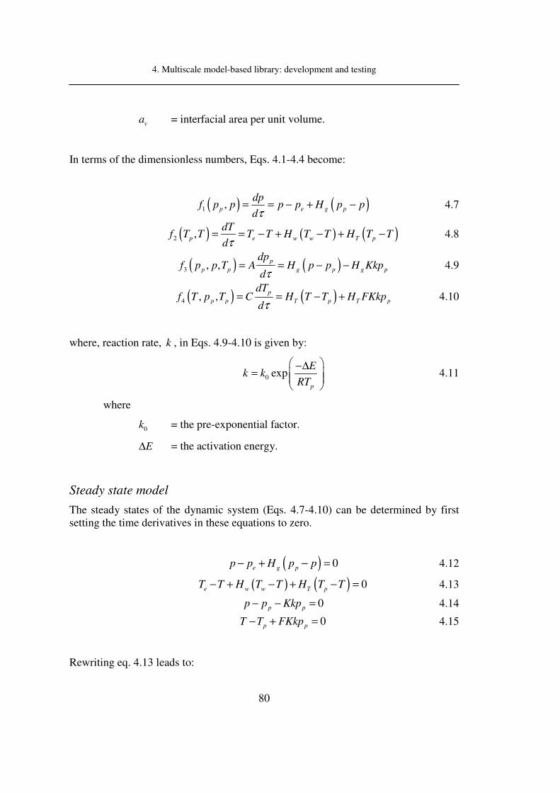
4. Multiscale model-based library: development and testing
80
v
a = interfacial area per unit volume.
In terms of the dimensionless numbers, Eqs. 4.1-4.4 become:
( ) ( )1 ,p e g p
dpf p p p p H p p
dτ= = − + − 4.7
( ) ( ) ( )2 ,p e w w T p
dTf T T T T H T T H T T
dτ= = − + − + − 4.8
( ) ( )3 , ,p
p p g p g p
dpf p p T A H p p H Kkp
dτ= = − − 4.9
( ) ( )4 , ,p
p p T p T p
dTf T p T C H T T H FKkp
dτ= = − + 4.10
where, reaction rate, k , in Eqs. 4.9-4.10 is given by:
0 expp
Ek k
RT
−∆=
4.11
where
0k = the pre-exponential factor.
E∆ = the activation energy.
Steady state model
The steady states of the dynamic system (Eqs. 4.7-4.10) can be determined by first setting the time derivatives in these equations to zero.
( ) 0e g p
p p H p p− + − = 4.12
( ) ( ) 0e w w T p
T T H T T H T T− + − + − = 4.13
0p pp p Kkp− − = 4.14
0p pT T FKkp− + = 4.15
Rewriting eq. 4.13 leads to:

4. Multiscale model-based library: development and testing
81
1
e T p W W
T W
T H T H TT
H H
+ +=
+ + 4.16
Combining Eqs. 4.12 and 4.14 gives,
( )1 1
ep
g
pp
H Kk=
+ + 4.17
Finally combining Eqs. 4.15, 4.16 and 4.17, the following equations are obtained
( )( )
( )
*1, ( )
1
( )1 1
W p
I
T W
eII
H T TQ a
H H
FKkpQ b
Hg Kk
+ −=
+ +
=+ +
4.18
where
( )
( )*
1
e W
W
T H TT
H
+=
+ 4.19
At the steady state I II
Q Q= .
Stability Analysis
The most common way to check the stability for a nonlinear set of differential equations (4.12-4.15) is through the linearization of the set of equations at a specific point of time or condition, followed by analysis of the eigenvalues of the Jacobian matrix. The linearized equations can be written in terms of the vector of disturbances from the steady state to obtain the Jacobian matrix, for example,

4. Multiscale model-based library: development and testing
82
( )
31 2 4
31 2 4
, , ,31 2 4
31 2 4
p pf p T p T
p p p p
p p p p
ff f f
p p p p
ff f f
T T T TJ
ff f f
p p p p
ff f f
T T T T
∂∂ ∂ ∂ ∂ ∂ ∂ ∂
∂∂ ∂ ∂ ∂ ∂ ∂ ∂ =
∂∂ ∂ ∂ ∂ ∂ ∂ ∂
∂∂ ∂ ∂ ∂ ∂ ∂ ∂
4.20
The eigenvalues for the above Jacobian matrix are obtained by setting the determinant of the matrix equal to zero;
11 13
22 24
31 33 34
42 43 44
0 0
0 00
0
0
b b
b b
b b b
b b b
λ
λ
λ
λ
− − = −
−
4.21
Solution of Eq. 4.21 in terms of eigenvalues, λ , is obtained from the roots of the following polynomial.
4 3 2 1 0b b b bI II III IVλ λ λ λ+ + + + = 4.22
Where,
( )
( ) ( )
( )
( )
( )
11 22 33 44
11 22 33 44 22 33 44 33 44
13 31 34 43
11 22 33 22 44 33 44 24 42 34 43
22 13 31 33 44 34 43 24 33 42
13 31 44
11 22 33 44 34 43 13 31 24
b
b
b
b
I b b b b
II b b b b b b b b b
b b b b
b b b b b b b b b b b
III b b b b b b b b b b
b b b
IV b b b b b b b b b
= − + + +
= + + + + +
− −
+ + − − +
= − + − + + +
= − + ( )42 22 44
11 24 33 42
b b b
b b b b
−
−
4.23
The values of ij
b in Eq.4.23 are listed in Table 4-1.

4. Multiscale model-based library: development and testing
83
The criterion to analyze the stability of the set of equations based on the eigenvalues, is that the eigenvalues must all have negative real parts (with or without an imaginary part) for the system to be stable. If any of the eigenvalues has a positive real part (with or without an imaginary part) the system is unstable.
Table 4-1 Values for expression 4.23.
bij
11b ( )1g
H− +
13b gH
22b ( )1T w
H H− + +
24b TH
31b gH A
33b ( )1 /g g p
H Kk A H p Ap− + = −
34b ( )2 2
g p p g p pH EKkp RT H E T T ART F− ∆ = ∆ −
42b TH C
43b ( )T T p pFH Kk C FH p p Cp= −
44b ( )2 21 1T T
p p
p p
H HE EFKkp T T
C RT C RT
∆ ∆− = − −
Many other criteria might be applied to analyze the stability of oscillating systems, for example, Routh theorem, Routh-Hurwitz criterion, Lienard-Chipart criterion, etc. (Gantmacher, 1960).
The results from the stability analysis obtained from the solution of the above equations are given in section 4.1.4 (page 89) of this chapter.

4. Multiscale model-based library: development and testing
84
Multiscale Model Analysis
A detailed explanation and comprehension of the phenomena of the batch catalytic fluidized bed reactor can be obtained through a systematic multiscale model-based analysis. This systematic approach helps to understand and solve the model equations such that the behaviour of the reactor at different scales of size can be generated and analyzed.
Figure 4.2 illustrates the multiscale representation of the various modelling options for a batch catalytic fluidized bed reactor. The unit operation scale of characteristic length between 1 – 10-1 m involves mass volume balances of the compounds and the particles inside the reactor; energy balance for compounds and also heat transfer surfaces inside or outside of the reactor (depending on the reactor configuration). In reality, it might be possible to describe the temperature axial dispersion but usually a uniform temperature is considered in the reactor. The size of the pellets can differ, which is the main reason why at this scale, the use of a stochastic pellet size distribution within the catalytic bed is recommended (characteristic length 10-2 – 10-4 m). The performance of a single catalyst pellet might also be considered (characteristic length 10-5 – 10-6 m). Using this option allows one to represent the complete behaviour of the catalyst bed inside the reactor. It is also possible to consider even smaller scales, for example, the performance inside the catalyst particle at a scale of 10-7 – 10-9 m. Generally, mass transfer phenomena have relevance in catalyst based chemical reactions, due to diffusion from the bulk-mass to the catalyst surface, diffusion of the reactants inside the pores, chemical adsorption on the wall of the catalyst (at the catalyst surface).
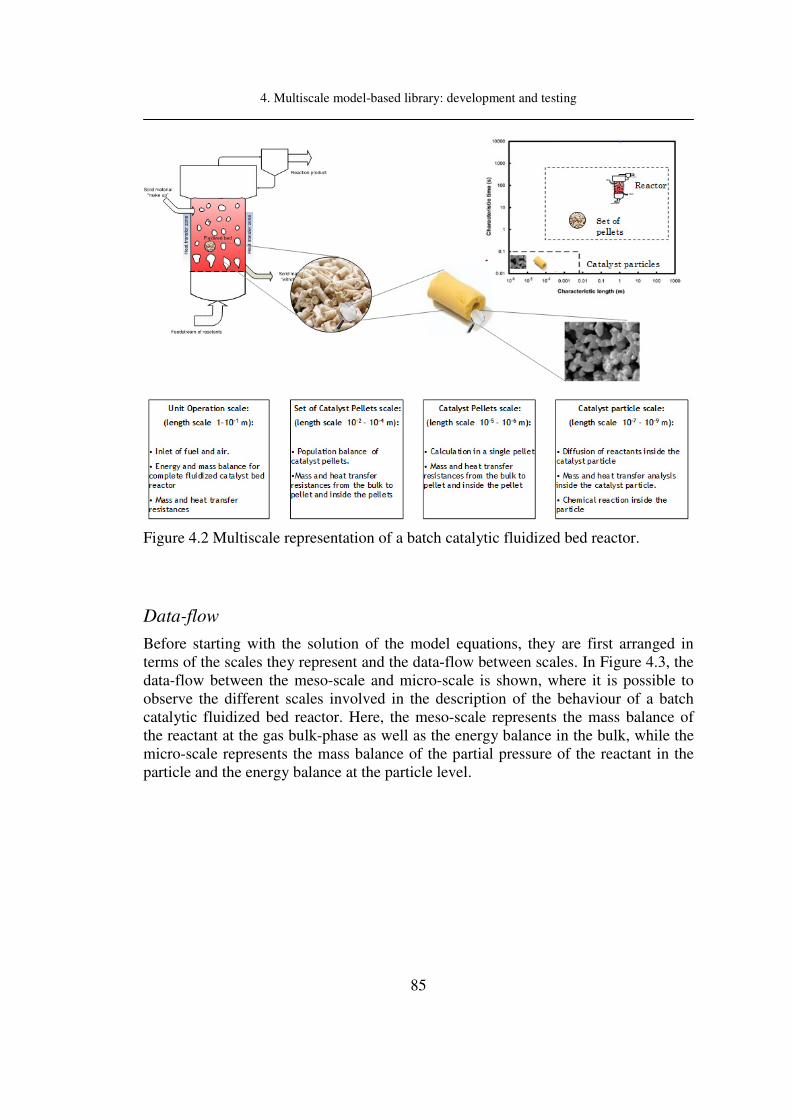
4. Multiscale model-based library: development and testing
85
Figure 4.2 Multiscale representation of a batch catalytic fluidized bed reactor.
Data-flow
Before starting with the solution of the model equations, they are first arranged in terms of the scales they represent and the data-flow between scales. In Figure 4.3, the data-flow between the meso-scale and micro-scale is shown, where it is possible to observe the different scales involved in the description of the behaviour of a batch catalytic fluidized bed reactor. Here, the meso-scale represents the mass balance of the reactant at the gas bulk-phase as well as the energy balance in the bulk, while the micro-scale represents the mass balance of the partial pressure of the reactant in the particle and the energy balance at the particle level.

4. Multiscale model-based library: development and testing
86
Figure 4.3 Data-flow for the batch catalytic fluidized bed reactor.
Data-flow from meso-scale to micro-scale consists of information related to the partial pressure of the reactant and the temperature in the bulk phase. This information is used in the micro-scale model, which returns the information about the partial pressure of the reactant and temperature in the particle to the meso-scale level. The information that is transferred between the scales corresponds to the same dynamic state. This kind of multiscale modelling problem can be classified as the multidomain integration framework. On the other hand, if the micro-scale model describes a set of particles with different characteristics (e.g. size), the equations describing the set of particles will be solved for each particle during the macro-scale solution of the model. This kind of multiscale modelling problem is classified as the embedded integration framework.
4.1.4. Model solution and analysis of results
The batch catalytic fluidized bed reactor model described above has been implemented in ICAS-MoT. This modelling tool is able to perform a model analysis in terms of the degrees of freedom, singularity, etc., of the set of model equations, thus, supporting the user in the solution of the mathematical problem.
Model analysis
The solution of the catalytic fluidized bed reactor model has also been carried out
Micro-scale
Meso-scale
p
T
pp
pT
( ) ( )1 ,p e g p
dpf p p p p H p p
dτ= = − + −
( ) ( ) ( )2 ,p e w w T p
dTf T T T T H T T H T T
dτ= = − + − + −
( ) ( )3 , ,p
p p g p g p
dpf p p T A H p p H Kkp
dτ= = − −
( ) ( )4 , ,p
p p T p T p
dTf T p T C H T T H FKkp
dτ= = − +

4. Multiscale model-based library: development and testing
87
using ICAS-MoT. Figure 4.4 illustrates the path that the modelling tool has taken for the solution of the model equations.
Figure 4.4 Work-flow and tools used from ICAS-MoT for catalytic fluidized bed reactor model.
After the model equations have been exported to ICAS-MoT, it performs model translation, analysis and verification; the software then solves the model equations by employing the appropriate solver for algebraic equations (AEs), differential algebraic equations (DAEs), partial differential algebraic equations (PDAEs); then, results are analyzed and validated, and then a model object is created (which can also be implemented in other simulation environments) as the final step of the modelling tool.
Model Simulation and results.
The data (input) needed to solve model equations (steady state and dynamic) are taken from Luss & Amudson (1968), and listed in Table 4-2.

4. Multiscale model-based library: development and testing
88
Table 4-2 Data for simulation study (Luss & Amudson, 1968).
Property Value Property Value
va
2
3500
ft
ft
w
T 720 R°
sc 0.2
BTU
lb F° α 0.4
gc 0.25
BTU
lb F° ε 0.7
gh 2
10
BTU
hr ft F° H−∆
48 10BTU
lb mol×
−
wh
230
BTU
hr ft F°
sρ
360
lb
ft
gk 2
1
lb mol
hr atm ft
− gρ
30.1
lb
ft
k 2
150002.5exp 20.7
lb mol
T hr atm ft
− −
A 0.17142
M 48lb
lb mol− C 205.74
P 1 atm F 8000
ep 0.1 atm gH 320
q V 375
lb
hr ft
TH 266
r 2 ft w
H 1.6
eT 600 R° Kk
150000.0006exp 20.7
T
−
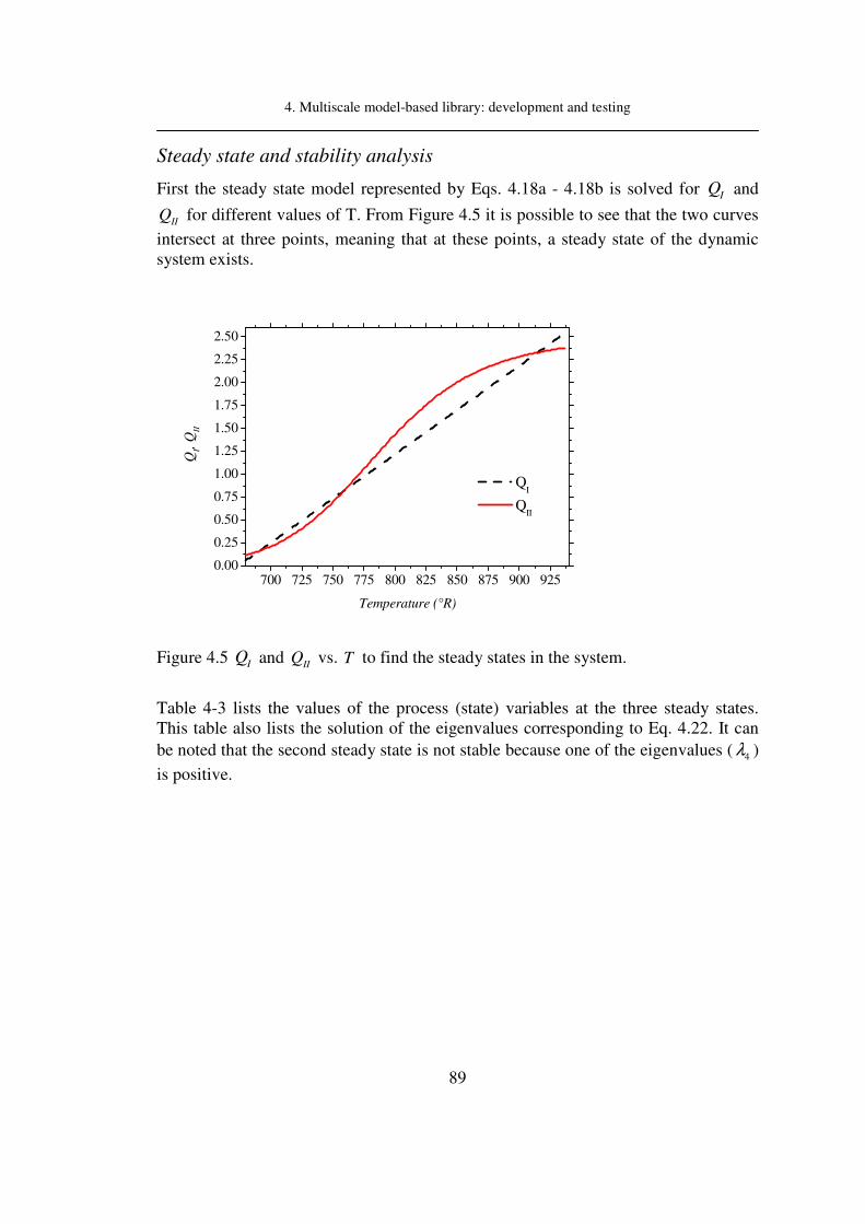
4. Multiscale model-based library: development and testing
89
Steady state and stability analysis
First the steady state model represented by Eqs. 4.18a - 4.18b is solved for IQ and
IIQ for different values of T. From Figure 4.5 it is possible to see that the two curves
intersect at three points, meaning that at these points, a steady state of the dynamic system exists.
700 725 750 775 800 825 850 875 900 9250.00
0.25
0.50
0.75
1.00
1.25
1.50
1.75
2.00
2.25
2.50
QI,
QII
Temperature (°R)
QI
QII
Figure 4.5 IQ and
IIQ vs. T to find the steady states in the system.
Table 4-3 lists the values of the process (state) variables at the three steady states. This table also lists the solution of the eigenvalues corresponding to Eq. 4.22. It can
be noted that the second steady state is not stable because one of the eigenvalues ( 4λ )
is positive.

4. Multiscale model-based library: development and testing
90
Table 4-3 Steady-state(SS) values for Simulation Study.
1st SS 2nd SS
(Not stable) 3rd SS
pp 0.0935 0.06694 0.00653
p 0.09352 0.06704 0.00682
pT 690.72 759.167 915.13
T 690.45 758.35 912.8
1λ -2187.2494513 -2189.306306 -2258.0244252
2λ -270.55715028 -270.5775586 -270.60246532
3λ -0.9120340679 -1.256116493 -12.560859964
4λ -6.4105069E-03 5.6925189E-03 -7.379499E-03
Dynamic behaviour analysis
The next step is to analyze the dynamic behaviour corresponding to each steady state. In this case, equations 4.7-4.10 are solved. Figure 4.6 shows the transient paths to the first steady state. The temperature of the bulk gas and the particles at the beginning of the operation are equal to 600 °R and 690.45 °R, respectively, while the partial pressure of the reactants at the particle at the beginning is zero, because no reactant is present at the start. The partial pressure of the reactant in the bulk gas is set to 0.1 atm at the start. These results confirm that the steady state is reached with the same values as given in Table 4-3. However, the steady state is not obtained at the same time for all the variables. For example, the steady state for partial pressure of the reactant (a) and temperature (c) of bulk gas and reactant partial pressure in the particles (b) are found quickly; while for particle temperature (d), this steady state is reached around
1000τ = .

4. Multiscale model-based library: development and testing
91
0 200 400 600 800 1000 12000.084
0.086
0.088
0.090
0.092
0.094
0.096
0.098
0.100
0.102
Par
tial
pre
ssure
of
reac
tant
in t
he
gas
ph
ase
(atm
)
Time (hr)
Partial pressure of reactant in the gas phase
0 200 400 600 800 1000 1200
0.00
0.02
0.04
0.06
0.08
0.10 Partial pressure of reactant in the particle
Par
tial
pre
ssure
of
reac
tant
in t
he
par
ticl
e (a
tm)
Time (hr)
0 200 400 600 800 1000 1200
600
620
640
660
680
700
Gas
phas
e te
mp
erat
ure
(°R
)
Time (hr)
Gas phase temperature
0 200 400 600 800 1000 1200
690.0
690.1
690.2
690.3
690.4
690.5
Par
ticl
e te
mper
ature
(°R
)
Time (hr)
Particle temperature
Figure 4.6 Model solution for steady state at lowest temperature.
The plots of the transient paths shown in Figure 4.7 corresponds to the third steady state (highest temperature). Again, the same trend can be obtained.
(a)
(b) (c)
(d)
0 2 4 6 8 10 12 14 16 180.084
0.086
0.088
0.090
0.092
0.094
0.096
0.098
0.100
0.102
Par
tial
pre
ssure
of
reac
tan
t in
th
e g
as p
has
e (a
tm)
Time (hr)
0 2 4 6 8 10 12 14 16
0.00
0.02
0.04
0.06
0.08
0.10
Time (hr) 0.00 0.04 0.08 0.12 0.16
600
620
640
660
680
700
Time (hr)

4. Multiscale model-based library: development and testing
92
0 100 200 300 400 500 6000.00
0.02
0.04
0.06
0.08
0.10
Par
tial
pre
ssure
of
reac
tant
in t
he
gas
phas
e (a
tm)
Time (hr)
Partial pressure of reactant in the gas phase
0 100 200 300 400 500 6000.00
0.02
0.04
0.06
0.08
0.10
Partial pressure of reactant in the particle
Par
tial
pre
ssure
of
reac
tant
in t
he
par
ticl
e (a
tm)
Time (hr)
0 100 200 300 400 500 600
600
650
700
750
800
850
900
Gas
phas
e te
mper
ature
(°R
)
Time (hr)
Gas phase temperature
0 100 200 300 400 500 600914.0
914.5
915.0
915.5
916.0
916.5
Par
ticl
e te
mper
ature
(°R
)
Time (hr)
Particle temperature
Figure 4.7 Model solution for steady state at highest temperature.
The plots of Figure 4.8 show the transient path corresponding to the second steady state, where a pulse increment (300 R° ) of the entering temperature is performed from
time (τ ) 1400 to 1480. From the resulting simulated behaviour, it is possible to observe that second steady state, is not stable because the system does not return to
(a)
(b)
(c)
(d)
0.0 0.5 1.0 1.5 2.0 2.5 3.0 3.5 4.0 4.5 5.0 5.5 6.00.00
0.02
0.04
0.06
0.08
0.10
Par
tial
pre
ssure
of
reac
tan
t in
th
e gas
phas
e (a
tm)
Time (hr)
0 1 2 3 4 50.00
0.02
0.04
0.06
0.08
0.10
Time (hr)
0.00 0.05 0.10 0.15 0.20 0.25 0.30600
650
700
750
800
850
900
Time (hr)
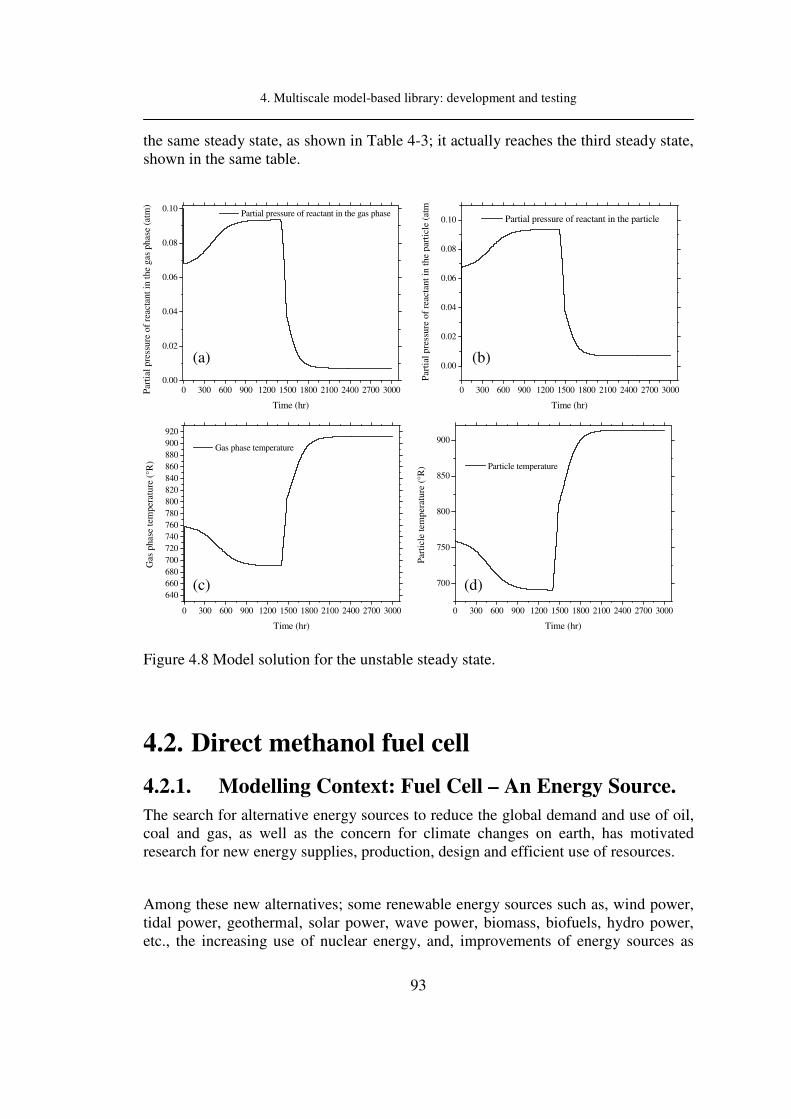
4. Multiscale model-based library: development and testing
93
the same steady state, as shown in Table 4-3; it actually reaches the third steady state, shown in the same table.
0 300 600 900 1200 1500 1800 2100 2400 2700 30000.00
0.02
0.04
0.06
0.08
0.10
Par
tial
pre
ssure
of
reac
tant
in t
he
gas
phas
e (a
tm)
Time (hr)
Partial pressure of reactant in the gas phase
0 300 600 900 1200 1500 1800 2100 2400 2700 3000
0.00
0.02
0.04
0.06
0.08
0.10 Partial pressure of reactant in the particle
Par
tial
pre
ssure
of
reac
tant
in t
he
par
ticl
e (a
tm)
Time (hr)
0 300 600 900 1200 1500 1800 2100 2400 2700 3000
640
660
680
700
720
740
760
780
800
820
840
860
880
900
920
Gas
phas
e te
mper
ature
(°R
)
Time (hr)
Gas phase temperature
0 300 600 900 1200 1500 1800 2100 2400 2700 3000
700
750
800
850
900
Par
ticl
e te
mper
ature
(°R
)
Time (hr)
Particle temperature
Figure 4.8 Model solution for the unstable steady state.
4.2. Direct methanol fuel cell
4.2.1. Modelling Context: Fuel Cell – An Energy Source.
The search for alternative energy sources to reduce the global demand and use of oil, coal and gas, as well as the concern for climate changes on earth, has motivated research for new energy supplies, production, design and efficient use of resources.
Among these new alternatives; some renewable energy sources such as, wind power, tidal power, geothermal, solar power, wave power, biomass, biofuels, hydro power, etc., the increasing use of nuclear energy, and, improvements of energy sources as
(a) (b)
(c) (d)

4. Multiscale model-based library: development and testing
94
fuel cells have been recognized as potential alternatives.
In this PhD-thesis a model-based analysis of the fuel cell has been performed. The objective here has been to highlight the use of multiscale modelling rather than an improved design of the fuel cell. A fuel cell is a device that is based on an electrochemical reaction to produce energy where the energy released from the chemical reaction is converted directly into electric power. Most recently, research in fuel cells has promoted it as an alternative energy source and storage for different applications, such as, automobiles, buses, cell phones, computers, etc. have been investigated (Cooper, 2007). Some advantages related to fuel cells as the future energy source are:
• High efficiencies
• Reduced air emission
• Extremely reliable
• Quiet operation
• Remote status monitoring
4.2.2. System (fuel cell) description
Fuel cells consist of an electrolyte sandwiched between two electrodes (see Figure 4.9). The fuel used in the operation is located on the anode side and chemical reaction is carried out in the catalyst layer of this side; oxidant (usually oxygen) is fed to the cathode side, which reacts with the ions allowed to cross through the electrolyte membrane. The electrons generated in the anode part of the cell are not allowed to pass through the membrane to the cathode side. So, these electrons must move through an electrical circuit to reach the other side of the cell.

4. Multiscale model-based library: development and testing
95
Figure 4.9 Fuel cells diagrams
Different types of fuel cells are classified in terms of the electrolyte employed, the kind of reaction taking place in the cell, the operation temperature range, the kind of catalyst required, the fuel required, and the mechanism of the charge conducted in it. Table 4-4 lists the different types of fuel cells.

4. Multiscale model-based library: development and testing
96
Table 4-4 Classification of different kind of Fuel cells (Cooper, 2007).
Efficiency
Operating temperature
Ion movement
Electrolyte Electrodes/
Catalyst
thermal output
Advantages Disadvantages
Lo
w-T
emp
erat
ure
Proton Exchange Membrane
40-47% 50-100°C H+ from anode to cathode
Solid organic polymer
Porous carbon coated with Pt catalyst
Warm water
- Solid electrolyte reduces corrosion and electrolyte management problems.
- Low temperature
- Quick start
- Requires expensive catalyst
- High sensitivity to fuel impurities
- Low temperature waste heat
-Waste heat temperature not suitable for combined-cycle.
Alkaline 50-60% 25-90°C OH- from cathode to anode
Alkaline solution (aqueous solution of potassium, etc)
Porous carbon coated with non-precious-metal catalyst
Warm water
- Cationic reaction faster in alkaline electrolyte, higher performance.
- Expensive removal of carbon dioxide from fuel and air streams required (carbon dioxide degrades the electrolyte)
Phosphoric Acid
~35% 150-220°C H+ from anode to cathode
Liquid phosphoric acid soaked in a matrix
Porous carbon coated with Pt catalyst
Hot
water
- Higher overall efficiency with combine-cycle mode.
-Increased tolerance to impurities in hydrogen.
- Requires expensive platinum catalysts
- Low current and power
- Large size/weight
Direct Methanol
25-40% 50-120°C H+ from anode to cathode
PEM (Solid polymer)
Anode: Pt/Ru; Cathode: Pt
Warm water
Liquid methanol is used directly
Not reforming required
- Methanol crossover from anode to cathode
- Presence of methanol in the cathode part reduces electricity output and waste methanol.
Hig
h-T
emp
erat
ure
Molten Carbonate
~55% 600-700°C CO3
-2 from cathode to anode
Ceramic matrix containing a molten carbonate
Catalyst: Ni
Anode: Ni or NiCr alloy
Cathode : NiO doped with Li
Steam
- High efficiency
- Fuel flexibility
-Can use a variety of catalyst
- Suitable for combined-cycle mode.
- High temperature speeds corrosion and breakdown of cell components
- Complex electrolyte management
-Slow start-up
Solid Oxide
45-50% 650-1000°C O-2 from cathode to anode
Matrix of yttria-stabilized zirconia; or ceria-gadolinium oxides
Perovskita: Material with similar structure as CaTiO3. General formula is ABO3.
Steam
- High efficiency
- Fuel flexibility
- Can use a variety of catalyst
- Suitable for combined-cycle mode
- Solid electrolyte reduces electrolyte management problems
- High temperature enhances corrosion and breakdown of cell components.
- Slow start-up
- Brittleness of ceramic electrolyte with thermal cycling

4. Multiscale model-based library: development and testing
97
4.2.3. Conceptualization of the model, development and
multiscale analysis
There are five main sections in fuel cells, which are: anode-channel compartment, anode catalyst layer, cathode-channel compartment, cathode catalyst layer and ion conducting membrane.
Anode-Channel Compartment
Fuel for the performance of the device is supplied through this compartment. When fuel is crossing the channel, part of the fuel is delivered to the catalyst layer of the fuel cell.
Anode Catalyst Layer
Due to the chemical reaction that is taking place and because of the presence of the catalyst, the generation of electrons and ions is performed in this component of the fuel cell. Mass transfer phenomena also play an important role in this section.
Cathode-Channel Compartment
The oxidant is passed through the cathode-channel; it is transported to the cathode catalyst layer, where, the oxidant performs a chemical reaction.
Cathode Catalyst Layer
The oxidant has a chemical reaction in this section of the fuel cell. Most of the time, the oxidant has a chemical reaction with the protons that are generated in the anode compartment.
Ion Conducting Membrane/Electrolyte
The electrolyte in the fuel cell plays one of the most important roles for the proper behaviour and efficiency of the device. This one allows the crossing of selected ions generated for the chemical reaction and avoids the transfer of electrons through it. So, electrons are passed through the electric circuit, generating an electrical current that is ready to be used. The electrolyte might be an appropriate membrane, a ceramic containing metallic compounds or even a liquid.

4. Multiscale model-based library: development and testing
98
Model Development
The development of the model is described in this section; it is based on the models proposed by Xu et al. (2005) and Sundmacher et al. (2001). Additional modelling details have been added to account for the mass balances in the cathode compartment and cathode catalyst layer. Firstly, the explanation of the mathematical equations explaining the different sections of the fuel cell is carried out. The different sections of the fuel cell are classified through the multiscale modelling framework. The anode- and cathode-channel compartment are in the meso-scale; while, the ion conducting membrane, and the anode and cathode catalyst layer are in the micro-scale.
Assumptions of the model
For the mathematical model for direct methanol the assumptions mentioned by Xu, et al. (2005) and Sundmacher, et al. (2001) have been taken into account and are listed below:
A1. The anode compartment is treated as a continuously stirred tank reactor (CSTR).
A2. The ohmic drops in current collectors and electric connections are negligible.
A3. Isothermal operation in the fuel cell.
A4. Oxygen is fed in excess, i.e., oxygen conversion in the cathode compartment is negligible, and therefore an oxygen mass balance is not required.
A5. Oxygen and carbon dioxide do not diffuse into the proton electrolyte membrane (PEM).
A6. The water concentration is assumed to be constant (excess component in liquid mixture).
A7. Mass transport resistances in the catalyst layers are negligible as these are thin (10 µm) in comparison to the diffusion layers (100 µm) and PEM (200 µm).
A8. Mass transfer coefficients of methanol and carbon dioxide in the anode diffusion layer are equal.
A9. The mixtures in the anode compartment and in the anode diffusion layer are treated as a pure liquid phase mixture, i.e., gas-phase formation, by release of carbon dioxide bubbles, is not taken into account.
A10. For other gas components (CO2, O2, N2) pure diffusion is assumed inside the membrane for reasons of simplicity. The mass transport in the membrane is source- and sink-free.
A11. The rate-determining step in the electrochemical methanol oxidation is the dissociative chemisorption of methanol on active platinum catalyst sides, so, formation of hydroxylic groups on the active ruthenium catalyst sites, surface

4. Multiscale model-based library: development and testing
99
reaction of the absorbed molecules and Surface reaction leading to the release of the reaction product carbon dioxide, are assumed to be at equilibrium; and, are used to determine the surface fraction covered by platinum.
A12. The entire methanol permeating through the PEM is totally oxidized.
Meso-scale
Anode-channel compartment
Mass balances for methanol and carbon dioxide for the anode channel compartment are described in this section. For the methanol mass balance, the concentration rate of change in the channel is described as:
( ) ( )3
3 3 3 3
1A
LSA SACH OH FA A A CLA
CH OH CH OH CH OH CH OHa
dc k Ac c c c
dt Vτ= − − − 4.24
where,
3
A
CH OHc = concentration of methanol in the anode compartment
( 3mol m ).
3
FA
CH OHc = feed concentration of methanol in the anode-channel
( 3mol m ).
3
CLA
CH OHc = concentration of methanol in the anode catalyst layer
( 3mol m ).
LSAk = mass transfer coefficient in the anode section ( m s ).
SAA = cross-sectional electrode area in the anode section ( 2
m ).
aV = anode compartment volume ( 3m ).
τ = resident mean time ( s ).
The left-hand term of equation 4.24 describes the change of methanol concentration in the anode channel compartment with respect to time. The first term on the right-hand side describes the change of methanol concentration with respect to the amount that is fed; the second term describes the mass transfer between the bulk and catalyst layer in the anode compartment.

4. Multiscale model-based library: development and testing
100
The mass balance for carbon dioxide that is generated during the chemical reaction is described as follows:
( ) ( )2
2 2 2 2
1A
LSA SACO FA A A CLA
CO CO CO COa
dc k Ac c c c
dt Vτ= − − − 4.25
where,
2
A
COc = concentration of carbon dioxide in the anode compartment
( 3mol m ).
2
FA
COc = feed concentration of carbon dioxide in the anode-channel
( 3mol m ).
2
CLA
COc = feed concentration of carbon dioxide in the anode catalyst
layer ( 3mol m ).
Equation 4.25 describes the rate of change of the carbon dioxide concentration to respect with time in the left-hand side of the equation. The first term on the right-hand side represents the change of carbon dioxide concentration with respect to the amount that is fed, while, the second term describes the mass transfer rate of this compound between the anode-channel compartment and the anode catalyst layer.
Cathode-channel compartment
Mass balances for the cathode compartment involve oxygen and water. The oxygen mass balance is represented as:
( ) ( )2
2 2 2 2
1C LSC SCO FC C C CLC
O O O O
c
dc k Ac c c c
dt Vτ= − − −
4.26
where,
2
C
Oc = concentration of oxygen in the cathode compartment
( 3mol m ).

4. Multiscale model-based library: development and testing
101
2
FC
Oc = feed concentration of oxygen in the cathode-channel
( 3mol m ).
2
CLC
Oc = concentration of oxygen in the cathode catalyst layer
( 3mol m ).
LSCk = mass transfer coefficient in the cathode section ( m s ).
SCA = cross-sectional electrode area in the cathode section ( 2
m ).
c
V = cathode compartment volume ( 3m ).
The left-hand term of equation 4.26 describes the rate of change of oxygen concentration with respect to time. The first terms of the right-hand side describes the change of oxygen concentration with respect to the amount that is fed, the second term describes the mass transfer between the bulk and the catalyst layer in the cathode compartment.
For water, the mass balance is written as,
( ) ( )2
2 2 2 2
1C LSC SCH O FC C C CLC
H O H O H O H O
c
dc k Ac c c c
dt Vτ= − − −
4.27
where,
2
C
H Oc = concentration of water in the cathode compartment
( 3mol m ).
2
FC
H Oc = feed concentration of water in the cathode-channel
( 3mol m ).
2
CLC
H Oc = feed concentration of water in the cathode catalyst layer
( 3mol m ).
Equation 4.27 is representing the rate of change of water concentration with respect to time on the left-hand side of the equation. The first term on the right-hand side represents the change of water concentration with respect to the amount that is fed, while, the second term describes the mass transfer rate of water between the cathode-channel compartment and the catalyst layer.
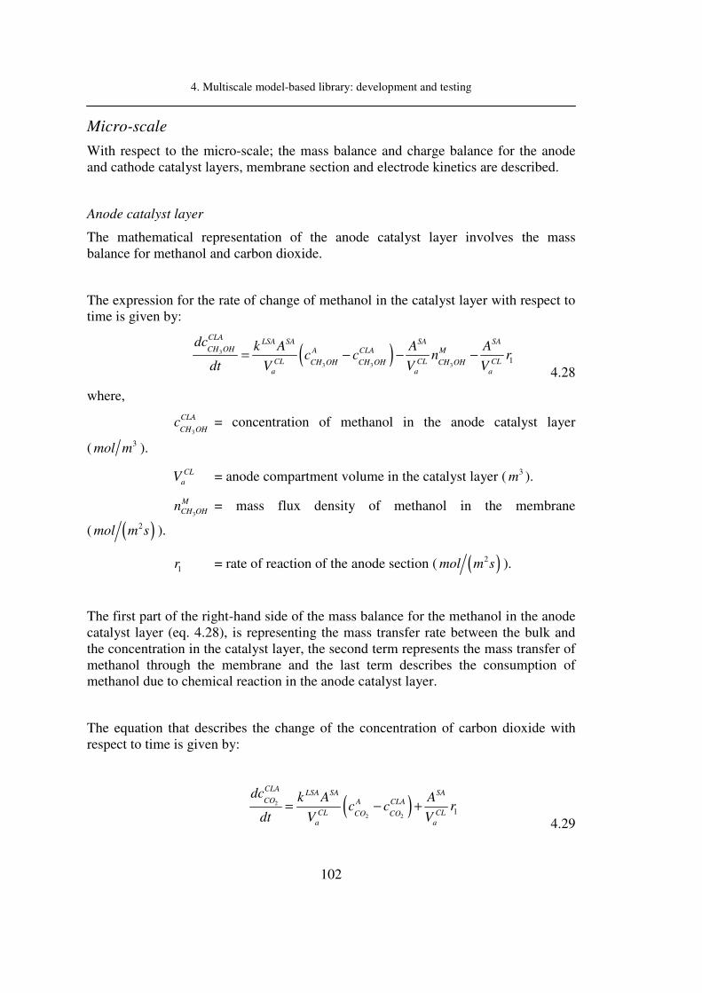
4. Multiscale model-based library: development and testing
102
Micro-scale
With respect to the micro-scale; the mass balance and charge balance for the anode and cathode catalyst layers, membrane section and electrode kinetics are described.
Anode catalyst layer
The mathematical representation of the anode catalyst layer involves the mass balance for methanol and carbon dioxide.
The expression for the rate of change of methanol in the catalyst layer with respect to time is given by:
( )3
3 3 31
CLALSA SA SA SA
CH OH A CLA M
CL CL CLCH OH CH OH CH OHa a a
dc k A A Ac c n r
dt V V V= − − −
4.28
where,
3
CLA
CH OHc = concentration of methanol in the anode catalyst layer
( 3mol m ).
CL
aV = anode compartment volume in the catalyst layer ( 3
m ).
3
M
CH OHn = mass flux density of methanol in the membrane
( ( )2mol m s ).
1r = rate of reaction of the anode section ( ( )2mol m s ).
The first part of the right-hand side of the mass balance for the methanol in the anode catalyst layer (eq. 4.28), is representing the mass transfer rate between the bulk and the concentration in the catalyst layer, the second term represents the mass transfer of methanol through the membrane and the last term describes the consumption of methanol due to chemical reaction in the anode catalyst layer.
The equation that describes the change of the concentration of carbon dioxide with respect to time is given by:
( )2
2 21
CLALSA SA SA
CO A CLA
CL CLCO COa a
dc k A Ac c r
dt V V= − +
4.29

4. Multiscale model-based library: development and testing
103
where,
2
CLA
COc = concentration of carbon dioxide in the anode catalyst layer
( 3mol m ).
The second mass balance in the anode catalyst layer (eq. 4.29) is for carbon dioxide that is representing the mass transfer rate between the concentration at the anode-channel and the catalyst layer. The last term of the equation is the rate of reaction that describes the generation of carbon dioxide in the catalyst layer.
The charge balance for the anode catalyst layer is given as;
( )1
16a
cell
a
di Fr
dt C
η= −
4.30
where,
a
η = electrode overpotential in the anode (V ).
celli =cell current density ( 2A m ).
a
C = double layer capacity in the anode ( 2F m ).
F = faraday constant 96485 C mol= .
Cathode catalyst layer
In the cathode catalyst layer section, the mass balance involves oxygen and water. For oxygen, the following equation is obtained:
( )2
2 25
CLCLSC SC SC
O C CLC
CL CLO Oc c
dc k A Ac c r
dt V V= − −
4.31
where,
2
CLC
Oc = concentration of oxygen in the cathode catalyst layer
( 3mol m ).
CL
cV = cathode compartment volume in the catalyst layer ( 3
m ).
5r = rate of reaction of the cathode section ( ( )2mol m s ).

4. Multiscale model-based library: development and testing
104
For water,
( )2
2 25
CLCLSC SC SC
H O C CLC
CL CLH O H Oc c
dc k A Ac c r
dt V V= − +
4.32
where,
2
CLC
H Oc = concentration of water in the cathode catalyst layer
( 3mol m ).
The left hand-side of equations 4.31 and 4.32 describe the rate of change of the concentrations of oxygen and water respectively, in the cathode catalyst layer; on the right-hand side, the first and second terms are involving the mass transfer from the cathode-channel to the catalyst layer and also the rate of consumption of oxygen ad water, respectively in the catalyst layer side.
The charge balance for the cathode catalyst layer is given by:
( )( )
35
16 Mc
cell CH OH
c
di F r n
dt C
η= − − +
4.33
where,
c
η = electrode overpotential in the cathode (V ).
3
M
CH OHn = mass flux density of methanol in the membrane
( ( )2mol m s ).
c
C = double layer capacity in the cathode ( 2F m ).
Equation 4.33 involves cell current density, mass flux of the crossover methanol as well as the kinetic reaction on the side of the cathode catalyst layer.
Membrane section
Description of membrane behaviour involves the mass balance for methanol through it.

4. Multiscale model-based library: development and testing
105
( )
( )( )3
3 3,
M
CH OHM M M
CH OH CH OH
c zn t z D vc z
z
∂= − +
∂ 4.34
where,
3
M
CH OHn = mass flux density of methanol in the membrane
( ( )2mol m s ).
3
M
CH OHc = concentration of methanol in the membrane ( 3mol m ).
MD = diffusion coefficient of methanol in membrane ( 2m s ).
v = flow velocity in membrane ( m s ).
Equation 4.34 is representing the transport of methanol through the membrane by diffusion and convection, where, convection in the membrane is driven by the electrostatic potential gradients and the pressure gradient. The flow velocity is given by:
( )( )
pM
H
M M
cell p c a pH c a
M M M
H H
k dpk dv c F
dz dz
i F c k p p d kk p p
D RT c k d
φ
φ
φ
φ
µ µ
µ
µ µ µ
+
+
+ +
= − −
+ − −= −
+
4.35
where,
kφ = electrokinetic permeability of membrane ( 2m ).
µ = pore fluid viscosity in membrane ( ( ) Kg m s ).
M
Hc + = proton concentration in membrane ( 3mol m ).
M
HD + = diffusion coefficient of methanol in membrane ( 2m s ).
F = Faraday constant ( C mol ).
cell
i = cell current density ( 2A m ).
Md = thickness of membrane ( m ).
c
p = pressure in cathode compartment ( Pa ).
ap = pressure in anode compartment ( Pa ).

4. Multiscale model-based library: development and testing
106
R = universal gas constant ( ( ) J mol K ).
Since the velocity v does not depend on the methanol concentration, Eq. 4.34 is a simple linear differential equation which can be solved analytically. Taking into account that the methanol concentration in the cathode catalyst layer is zero due to instantaneous methanol oxidation at the cathode, one obtains the following expression for the steady-state methanol mass flux density in the membrane:
( )
( )3 3
exp
exp 1
MM CLA
CH OH CH OHM
Pe PeDn c
d Pe=
− 4.36
where the Peclet number Pe is defined as follows:
M
M
vdPe
D= 4.37
where,
MD = diffusion coefficient of methanol in membrane ( 2m s ).
Md = thickness of membrane ( m ).
Electrode Kinetics
Two kinds of chemical reactions are identified in the performance of the direct methanol fuel cell, one on the anode side and the other on the cathode side.
Firstly, the kinetic expressions for anodic methanol oxidation are explained. This electrochemical oxidation of methanol is carried out on the platinum-ruthenium catalyst and consists of 4 reaction steps:
(R1) 3 33 3 3Pt CH OH Pt COH H e+ −+ ↔ − + +
(R2) 23 3 3 3 3Ru H O Ru OH H e+ −+ ↔ − + +
(R3) 3 22 2 2Pt COH Ru OH Pt COOH H O Pt Ru− + − ↔ − + + +
(R4) 2 2Pt COOH Ru OH CO H O Pt Ru− + − ↔ + + +

4. Multiscale model-based library: development and testing
107
The first (and rate-determining) step is the dissociative chemisorption of methanol on active platinum catalyst sites (R1) and it is represented by;
3
311 1
1
1exp expCLA
a Pt a Pt COHCH OH
F Fr k c
RT K RT
αη θ η θ −
= − −
4.38
The rate of formation of hydroxylic groups on the active ruthenium catalyst sites (R2) is given by:
22 2
2
1exp exp
a Ru a Ru OH
F Fr k
RT K RT
αη θ η θ −
= − −
4.39
The rate if the surface reaction (R3) of the absorbed molecules formed in the previous steps
3
2 2 2
3 3
3
1Pt COH Ru OH Pt COOH Pt Ru
r kK
θ θ θ θ θ− − −
= −
4.40
The rate of the surface reaction leading to the release of the reaction product carbon dioxide (R4) is represented by:
24 4
4
1 CLA
Pt COOH Ru OH CO Pt Rur k c
Kθ θ θ θ− −
= −
4.41
As far as oxygen reduction is concerned (R5), it is occurring on the cathode side; the expression of the rate of consumption is the following:
(R5) 2 23 2 6 6 3O H e H O+ −+ + ↔
2
3/ 2
55 5 0
exp 1 expO
c c
pF Fr k
RT RT p
αη η
= − − 4.42

4. Multiscale model-based library: development and testing
108
Since the reaction steps (R2)-(R4) are assumed not to be rate determining, their driving forces nearly vanish. Then, the combination of these equations is giving:
( )2 2 2
42
3 12 4 2 3
32
12 3 4
exp
exp 0
CLA CLA CLA
Pt a PtCO CO CO
a
Fc K K c K K c
RT
FK K K
RT
αθ η θ
αη
+ + −
=
4.43
where,
i
k = rate constant of reaction i ( ( )2mol m s ).
α = charge transfer coefficient.
T = cell temperature ( K ).
Pt
θ = surface fraction covered by Pt.
3Pt COH
θ − = surface fraction covered by Pt3-COH.
Ru
θ = surface fraction covered by Ru.
Ru OH
θ − = surface fraction covered by Ru-OH.
Pt COOH
θ − = surface fraction covered by Pt-COOH.
2O
p = partial pressure of oxygen ( Pa ).
0p = pressure at standard conditions ( Pa ).
where 2O
p is defined is represented by:
2
% c Oxigen in airO
p p= 4.44
where,
c
p = Pressure in the cathode compartment ( Pa ).
4. Multiscale model-based library: development and testing
109
Overall cell voltage and mass transfer coefficients
The performance of the direct methanol fuel cell is observed through the calculation of the cell voltage,
Mstd cell
cell cell a c M
i dU U η η
κ= − + −
4.45
where,
cell
U = total cell voltage (V ).
std
cellU = standard cell voltage (V ).
cell
i = cell current density ( 2A m ).
Md = thickness of membrane ( m ).
Mκ = conductivity of membrane ( 1 1m
− −Ω ).
As far as the mass transfer coefficients are concerned, their values can be determined from measured limiting current densities limi . At the steady state, time derivatives in
equations 4.24, 4.25, 4.28, 4.29, 4.30 and 4.33 approach zero at the limiting current, and also the methanol concentration in the anode catalyst layer approaches zero. Under these conditions equations 4.24, 4.28 and 4.30 are combined to give:
3
lim
lim6
FLSA
F F SA
CH OH
V ik
FV c A i=
− 4.46
where,
FV = anode feed flow rate ( minml ).
limi = limit cell current density ( 2A m ).
The main phenomena occurring in the development of the model are described below:
• Convective mass transport in the anode cell compartment.
• Electrochemical oxidation of methanol in the anode catalyst layer.
• Electrochemical reduction of oxygen in the cathode catalyst layer.

4. Multiscale model-based library: development and testing
110
• Mass transfer of methanol and carbon dioxide through the anode diffusion layer.
• Methanol crossover, i.e. the undesired transfer of methanol through the PEM by diffusion electroosmosis and pressure-driven transport.
• Undesired electrochemical oxidation of methanol at the cathode catalyst layer.
Taking into account the assumptions and considering the main phenomena in the direct methanol fuel cell, the set of differential algebraic equations (Eqs. 4.24-4.42) representing the fuel cell model is summarized in Table 4-5.

4. Multiscale model-based library: development and testing
111
Table 4-5 Direct methanol fuel cell multiscale mathematical model.
Scale Equation M
eso
-sca
le
Mas
s B
alan
ce
An
od
e co
mpar
tmen
t
( ) ( )3
3 3 3 3
1A
LSA SACH OH FA A A CLA
CH OH CH OH CH OH CH OHa
dc k Ac c c c
dt Vτ= − − −
( ) ( )2
2 2 2 2
1A
LSA SACO FA A A CLA
CO CO CO COa
dc k Ac c c c
dt Vτ= − − −
Mic
ro-s
cale
An
od
e C
atal
yst
Lay
er
( )3
3 3 31
CLALSA SA SA SA
CH OH A CLA M
CL CL CLCH OH CH OH CH OHa a a
dc k A A Ac c n r
dt V V V= − − −
( )2
2 21
CLALSA SA SA
CO A CLA
CL CLCO COa a
dc k A Ac c r
dt V V= − +
Mem
bra
ne
mo
del
( )( )3 3
exp
exp 1
MM CLA
CH OH CH OHM
Pe PeDn c
d Pe=
−
Char
ge
Bal
ance
s
An
od
e C
atal
yst
Lay
er
( )1
16a
cell
a
di Fr
dt C
η= −
Cat
ho
de
Cat
aly
st L
ayer
( )( )3
5
16 Mc
cell CH OHc
di F r n
dt C
η= − − +
Con
stit
uti
ve
Equ
atio
ns
Ele
ctro
de
kin
etic
s
3
311 1
1
1exp expCLA
a Pt a Pt COHCH OH
F Fr k c
RT K RT
αη θ η θ −
= − −
( )2 2 2
42
3 12 4 2 3
32
12 3 4 0
CLA CLA CLA
Pt a PtCO CO CO
a
Fc K K c K exp K c
RT
FK exp K K
RT
αθ η θ
αη
+ + −
=
2
3/ 2
55 5 0
exp 1 expO
c c
pF Fr k
RT RT p
αη η
= − −

4. Multiscale model-based library: development and testing
112
The second equation in the sub-classification Electrode kinetics in Table 4-5 is obtained as a result of assumption A11.
Multiscale Model Analysis
A detailed explanation and comprehension of the phenomena of the batch direct methanol fuel cell can be obtained through a systematic multiscale model-based analysis. This systematic approach helps to understand and solve the model equations such that the behaviour of the fuel cell at different scales of size can be generated and analyzed.
Figure 4.10 illustrates the multiscale representation of a fuel cell as well as the application of this device. Fuel cells might have different applicability, nowadays, some of the main applications are oriented to computers, automobiles, etc., and the prediction of the behaviour at this scale can be classified in the macro-scale level, which would give a general idea about the performance of the complete device. A model analysis in the meso-scale might be done, where, the behaviour of the catalyst and membrane layers can be predicted and analyzed. Further details can be investigated if there is an interest about learning more in the proton and electron scale. The modelling at this scale would help to understand the hydrogen proton diffusion, and ion transport between the cathode and anode, for example. In this way, it is feasible to have details at different scales of length and time.
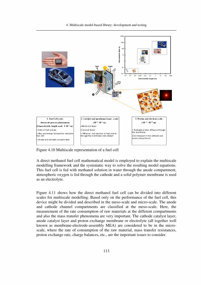
4. Multiscale model-based library: development and testing
113
Figure 4.10 Multiscale representation of a fuel cell
A direct methanol fuel cell mathematical model is employed to explain the multiscale modelling framework and the systematic way to solve the resulting model equations. This fuel cell is fed with methanol solution in water through the anode compartment, atmospheric oxygen is fed through the cathode and a solid polymer membrane is used as an electrolyte.
Figure 4.11 shows how the direct methanol fuel cell can be divided into different scales for multiscale modelling. Based only on the performance of the fuel cell, this device might be divided and described in the meso-scale and micro-scale. The anode and cathode channel compartments are classified at the meso-scale. Here, the measurement of the rate consumption of raw materials at the different compartments and also the mass transfer phenomena are very important. The cathode catalyst layer, anode catalyst layer and proton exchange membrane or electrolyte (all together well known as membrane-electrode-assembly MEA) are considered to be in the micro-scale, where the rate of consumption of the raw material, mass transfer resistances, proton exchange rate, charge balances, etc., are the important issues to consider.

4. Multiscale model-based library: development and testing
114
Figure 4.11 Multiscale division for a fuel cell.
Data-flow
Data-flow between the different scales involved in the multiscale model direct methanol fuel cell is highlighted in Figure 4.12. This multiscale model is employing the multidomain framework.

4. Multiscale model-based library: development and testing
115
Figure 4.12 Data-flow for the direct methanol fuel cell between the different scales.
The anode-channel and cathode-channel compartments belong to the meso-scale, while, the membrane-electrode-assembly are considered to be in the micro-scale. Information that is transferred from the meso-scale to the micro-scale are the concentrations of methanol and carbon dioxide (at the anode side), and, concentrations of water and oxygen (at the cathode side). Information transferred from the micro-scale to the meso-scale are, methanol and carbon dioxide concentrations as well as their mass transfer coefficients that are coming from the anode catalyst layer, and, the oxygen and water concentration plus their mass transfer coefficients from the cathode catalyst layer.
The model equations at the two scales could be solved separately. For example, to
4. Multiscale model-based library: development and testing
116
solve the problem only at meso-scale, the information that is taken from micro-scale is known data. In this case, the multiscale model is classified as serial: simplification
(micro-scale) integration framework. Similarly solving the model at the micro-scale, information coming from the meso-scale might be considered as known data. The problem classification in this case serial: simplification (meso-scale) integration
framework. Another interesting feature to highlight for this direct methanol fuel cell model, is that the model calculations at a smaller scale, for example, adding a model for calculating the diffusion coefficient of methanol through the membrane medium requires a smaller scale than “micro”. That is, the calculation of the diffusion coefficient is performed via dynamic simulation, and the problem classification becomes serial: one way coupling integration. When experimental values of the diffusion coefficient are fitted in a correlation and values for the variable are taken from it, this integration could be classified as serial: simplification (nano-scale)
structure due to the order of magnitude of the calculation.
4.2.4. Model solution and analysis of results
Figure 4.13 illustrates a screenshot of ICAS-MoT. Here, the classification of the different type of variables is performed in this section of ICAS-MoT. In addition, the degree of freedom analysis that employs an incidence matrix, is illustrated in this step, where, the rows represent the equations of the mathematical model while the columns represent the variables of the complete model, the diagonal line marks if the variable is present or not in the corresponding equations as unknown variable. For this set of equations that consists of 6 differential equations and 1 algebraic equation, it is necessary to specify the initial values for the 6 dependent variables associated to the 6 differential equations, in addition to the values of temperature, pressure in the anode and cathode, and the cell current value. The rest of the variables involved in the mathematical models, are classified as parameters, except for the variable
representing the surface fraction covered by Pt ( Ptθ ) that is solved through the single
algebraic equation.

4. Multiscale model-based library: development and testing
117
Figure 4.13 Analysis of degrees of freedom through the use of ICAS-MoT.
Model Simulation and results
Solution of the model equations (from Table 4-5) is done using ICAS-MoT and has been done in a special manner; because external software is connected with ICAS-MoT to be used as user interface.
The work-flow for the solution of the mathematical model is shown in Figure 4.14, and starts with the introduction of the mathematical model to ICAS-MoT, which performs a translation, analysis and verification of the model; subsequently, a solution administrator is called; as it is mentioned above, an external software is employed as a user interface (employing ICAS-Mot as modelling engine) that is connected with ICAS-MoT though the use of COM-objects. Finally, the validation and implementation of results is carried out.

4. Multiscale model-based library: development and testing
118
Figure 4.14 Work-flow and tools employed for the solution of the direct methanol fuel cell.
The solution of the model equations is done with the aim of highlighting the advantages of employing a multiscale model analysis. The simulation results highlight the differences that can be observed when more details are considered as well as the way the resulting mathematical model is solved. Table 4-6 gives the values of the variables that are specified for the solution of the model equations.

4. Multiscale model-based library: development and testing
119
Table 4-6 Data for the direct methanol fuel cell model.
Property Value Property Value
3
FA
CH OHc
3500 mol m α 0.5
2
FA
COc
30 mol m aC 240000 F m
3 ,
CLA
CH OH initialc
30 mol m cC 2100000 F m
2 ,
CLA
CO initialc
30 mol m Md 0.0002 mµ
,a initialη 0 V pk 18 21.57 e m−
,c initialη 0 V µ ( )0.0003353 Kg m s
T 343.15 K kφ 19 21.13 e m−
cp 300000 Pa m
Hc + 31200 mol m
ap 100000 Pa M
HD + 09 25.4e m s
−
celli 240 A m M
D 10 22.9 e m s−
1k 07 24.9e mol m s− τ 500 s
5k 07 21.8e mol m s−
SAA 20.0009 m
1K 1 aV 05 31.15 e m
−
2K 0.5 CL
aV 07 34.0 e m−
3K 1 std
cellU 1.2 V
4K 0.7 Mκ ( )
117 m
−Ω
FV 1.36 minml limi 21150 A m
0p 101325 Pa R 8.314 J Kmol

4. Multiscale model-based library: development and testing
120
In order to show what the differences are when the model is multiscale or single (higher) scale, the model is included in Table 4-5 is solved for the analysis. Two different scenarios have been considered:
1) Multiscale modelling framework (MS): The entire set of equations listed in Table 4-5 is solved (multidomain integration structure), that is, the meso-scale and micro-scale are taken into account simultaneously. The variables that both scales are sharing during the calculations are listed in Table 4-7:
Table 4-7 Variables shared between meso-scale and micro-scale.
Property Value
Methanol bulk concentration 3
A
CH OHc
Concentration in the catalyst layer of methanol 2
A
COc
Carbon dioxide bulk concentration 3
CLA
CH OHc
Concentration in the catalyst layer of carbon dioxide 2
CLA
COc
2) Single scale modelling framework (SS): This scenario concerns only the solution of the meso-scale equations listed in Table 4-5. For the micro-scale equations, values of the dependent and explicit variables are specified. In this case study, the values are taken from the multiscale steady state simulation. This calculation can be termed as serial: simplification (micro-scale) structure (also called single scale calculation).
Figure 4.15 illustrates the methanol concentration at the meso-scale. One curve describes the behaviour of methanol concentration involving multiscale modelling that is indicated by MS (meso-scale and micro-scale), while, the other is showing the behaviour using only meso-scale as it is explained in scenario 2 (SS). Evidently, both of the scenarios ought to give the same steady state values because they represent methanol concentration at the meso-scale. However, the pathways to achieve them are different as it can be noted from the trends of both curves. With respect to multiscale calculations, a higher level of detail is covered during the calculations as the meso-scale and micro-scale models are being solved simultaneously.

4. Multiscale model-based library: development and testing
121
0 500 1000 1500 2000 2500 3000 3500 4000
486
488
490
492
494
496
498
500
502
CC
H3O
H , m
ol/
m3
Time, s
SS
MS
Figure 4.15 Methanol concentration with multiscale modelling and single scale modelling.
The calculated concentrations of carbon dioxide at the meso-scale are illustrated in Figure 4.16, and it is also seen that although the same steady state is reached, the path to reach them is different for both approaches.
0 500 1000 1500 2000 2500 3000 3500 4000
0.0
0.5
1.0
1.5
2.0
2.5
3.0
SS
MS
CC
O2
, m
ol/
m3
Time, s
Figure 4.16 Carbon dioxide concentration with multiscale modelling and single scale modelling.
4. Multiscale model-based library: development and testing
122
4.3. Microcapsule for controlled release of
active ingredients
Microcapsules are the products of the microencapsulation that basically consists of the wrapping of substances (one playing the role of active ingredient and the other solvent medium) in another substance (shell of the microcapsule). Microcapsules usually have a spherical shape on a small size scale, where the wall/shell of the microcapsule regularly envelops the core that consists of the active ingredient and solvent. In some cases, however, the droplets of the active ingredient plus solvent medium are dispersed in the complete body of the microcapsule, where the phase of the active ingredient and/or solvent might be liquid or gas.
Controlled release can be defined as one technology that involves a product (a device) that is specifically designed to provide the delivery of an active ingredient to a specific target and with a desired rate and duration.
Initially, microcapsules for controlled release of active ingredients were developed for applications in the products from the pharmaceutical industry. However, the application of microcapsules has been widely extended to a broad variety of industries, such as, cosmetics, agrochemicals, consumer and personal care products, industrial chemical, biotechnology, food, biomedicals, sensors, etc., which have contributed to the research work in this field. Microencapsulation of active ingredients is a multidisciplinary task; for instance, the application of this activity in pharmaceuticals might require the scientific knowledge of experts in physics, physiology, biology, pharmacology, and, chemistry, also supported by modelling know-how where chemical engineering plays an important role.
In general the methods of microencapsulation can be broadly classified in two groups: physical methods and chemical methods. For example,
• Physical methods: Pan coating, fluid bed coating, centrifugal head coextrusion, rotary disk atomization, stationary nozzle coextrusion, spray chilling, spray drying, submerged nozzle coextrusion, etc.
• Chemical methods: interfacial polymerization, solvent evaporation, solvent extraction, in-situ polymerization, complex and simple coacervation, liposome technology, nanoencapsulation, phase separation, etc.

4. Multiscale model-based library: development and testing
123
The ingredients used for the microcapsule, particularly the active ingredient and solvent, are certainly related with the needs of the product, but the wall/shell of the microcapsules in general might be synthetic and natural polymers (the most used), proteins, fats, polysaccharides, waxes, resins, starches, etc.
This section of the thesis provides a description of the mathematical model of microcapsules for controlled release of active ingredients from the pharmaceutical and pesticide industries.
4.3.1. Modelling context: Microcapsule for controlled
release of pesticides and pharma-products.
In the agrochemical industry, the use of controlled release technology for the delivery of pesticides to the environment has numerous advantages: from optimized delivery of the active ingredients, to reduction of hazards to humans and environment. That is, the amount of pesticide used on the field can be reduced and also the safety level during its use can be improved. As far as controlled release of drugs or pharma-products is concerned, this technology is mainly aimed at controlling the amount of the drug delivered. The main benefits of controlled release are that it helps to keep an effective level of drug in the body for a specific period of time, and thereby, side effects generated by drug overdosing and/or under-dosing may be avoided.
Figure 4.17 illustrates one of the most common trends in the release of products (either pesticides or pharmaceuticals) as well as the desired lower and upper limits of the delivered product. The lower limit in Figure 4.17 represents the minimum non-toxic concentration, while the upper line represents the maximum effective concentration of the active ingredient. The dashed line curve represents an example of release without a device (for controlled release) while the continuous line is an example of controlled release through a device within specified limits. The behaviour described above can be generated by employing different models for controlled release of the active ingredient.
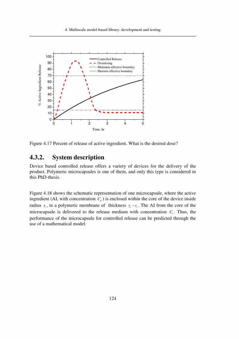
4. Multiscale model-based library: development and testing
124
0 1 2 3 4 50
10
20
30
40
50
60
70
80
90
100 Controlled Release
Overdosing
Minimum effective boundary
Maxium effective boundary
% A
ctiv
e In
gre
die
nt
Rel
ease
Time, hr
Figure 4.17 Percent of release of active ingredient. What is the desired dose?
4.3.2. System description
Device based controlled release offers a variety of devices for the delivery of the product. Polymeric microcapsules is one of them, and only this type is considered in this PhD-thesis.
Figure 4.18 shows the schematic representation of one microcapsule, where the active ingredient (AI, with concentration dC ) is enclosed within the core of the device inside
radius ir , in a polymeric membrane of thickness o ir r− . The AI from the core of the
microcapsule is delivered to the release medium with concentration rC . Thus, the
performance of the microcapsule for controlled release can be predicted through the use of a mathematical model.
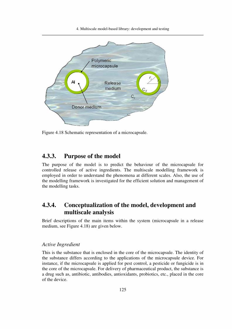
4. Multiscale model-based library: development and testing
125
Figure 4.18 Schematic representation of a microcapsule.
4.3.3. Purpose of the model
The purpose of the model is to predict the behaviour of the microcapsule for controlled release of active ingredients. The multiscale modelling framework is employed in order to understand the phenomena at different scales. Also, the use of the modelling framework is investigated for the efficient solution and management of the modelling tasks.
4.3.4. Conceptualization of the model, development and
multiscale analysis
Brief descriptions of the main items within the system (microcapsule in a release medium, see Figure 4.18) are given below.
Active Ingredient
This is the substance that is enclosed in the core of the microcapsule. The identity of the substance differs according to the applications of the microcapsule device. For instance, if the microcapsule is applied for pest control, a pesticide or fungicide is in the core of the microcapsule. For delivery of pharmaceutical product, the substance is a drug such as, antibiotic, antibodies, antioxidants, probiotics, etc., placed in the core of the device.

4. Multiscale model-based library: development and testing
126
Donor Medium
Usually, the active ingredients are solid substances that need to be dissolved in a solvent (donor medium).
Microcapsule wall (polymeric membrane)
The active ingredient together with the solvent is encapsulated by a polymeric membrane. One of the most important phenomena occurring here is the mass transfer of the active ingredient through this wall.
Release Medium
The active ingredient diffuses out from the microcapsules into the release medium. The medium depends of the application field; for instance, in the agrochemical field the most common release medium is water, while for a pharmaceutical product, the release medium could be gastric acid, blood, or any other medium found within the human body.
Model Development
A mathematical model (Muro-Suñé et al., 2005) representing the controlled release of active ingredients is employed for this case study. Multiscale modelling issues are considered. Three different scales have been identified: Nano-scale (calculation of diffusion coefficient), micro-scale (release of active ingredient in presented microcapsules), and meso-scale (normal distribution of microcapsules).
The model for predicting the behaviour of microcapsules for controlled release considers the following assumptions.
A1. Diffusion occurs through a film that is thin enough so that the diffusion can be considered one dimensional.
A2. Initial concentration of AI is equal for all the microcapsules.
A3. Diffusion coefficient is independent of concentration.
A4. Concentration can be affected for the diffusivity of the active ingredient into the polymer, and also, due to the partition coefficient between the wall of the microcapsule (polymeric membrane) and the donor and the receiver (release

4. Multiscale model-based library: development and testing
127
medium).
A5. Isothermal condition during the controlled release.
A6. Non-constant activity source.
A7. The model is applicable to systems where the active ingredient is available in solution below the solubility limit.
Nano-scale
This scale concerns the calculation of diffusion coefficients for which an extended version of the Zielinski and Duda (1992) and Vrentas et al. (1996) model, as presented by Muro Suñe (2005) is employed. The diffusion coefficient is calculated as follows:
( )
( ) ( )
* *
1 1 2 2
1 011 12
1 21 1 2 22 2
exp exp
g g
wV w VED D
K KRTw K T T w K T T
ξ
γ γ
− +− =
− + + − +
4.47
where,
1D = diffusion coefficient of AI in the polymer.
0D = constant pre-exponential factor.
E = energy (per mole) that the molecule needs to overcome attractive forces which constrain it to its neighbours.
R = gas constant.
T = temperature.
gi
T = glass transition temperature of compound i.
i
w = weight fraction of component i.
1 2,i i
K K = free volume parameter of compound i.
*
iV
= critical hole free volume required for a jump.
ξ = ratio of molar volumes for the solvent and the polymer
jumping units.
γ = overlap factor (between 0.5 and 1).

4. Multiscale model-based library: development and testing
128
If the necessary diffusion coefficient cannot be calculated through using equation 4.47, then values from open literature, from experiments or dynamic simulation could be used.
Micro-scale
Equations at the micro-scale represent the behaviour of one single microcapsule. These mathematical expressions describe the concentration of the active ingredient in the donor medium as well as in the release medium. The concentration profile is following Fick’s law of diffusion and has a dependence on the time. The concentration of the active ingredient in the donor is given by:
, / /
/ ,
, / ,
expd i i i m d m r r
m d d initial
d i r m d d i
dC DA DA K K VK C t
dt hV V h K V
= − − +
4.48
where,
,d iC = concentration of donor as function of time ( 3
g m ).
,d initialC = initial concentration of donor as function of time ( 3g m ).
/m dK = partition coefficient of the AI between the donor and the
polymer membrane.
/m rK = partition coefficient of the AI between the receiver and the
polymer membrane.
,d iV = donor volume ( 3
m ).
r
V = receiver volume ( 3m ).
iA = surface area through which diffusion takes place ( 2
m ).
D = polymer solvent binary mutual diffusion coefficient ( 2m s ).
h = thickness of the microcapsule wall ( m ).
t = time ( s ).
Equation 4.48 describes the change of the concentration of the active ingredient in the donor with respect to time.

4. Multiscale model-based library: development and testing
129
Analytical solution of equation 4.48 gives the following result:
/ , /
, , /
/ / , / ,
1 expm r d i i m r r
d i d initial m d
m d r m r d i r m d d i
K V DA K VC C K t
K V K V V h K V
= − − + +
4.49
The concentration of the active ingredient in the receiver (release medium) is given by:
, / /
/ ,
/ ,
exp r i i i m d m r r
m d d initial
r r m d d i
dC DA DA K K VK C t
dt V h V h K V
= − +
4.50
where,
,r iC = concentration of receiver as a function of time ( 3
g m ).
,d initialC = initial concentration of donor as function of time ( 3g m ).
/m dK = partition coefficient of the AI between the donor and the
polymer membrane.
/m rK = partition coefficient of the AI between the receiver and the
polymer membrane.
,d iV = donor volume ( 3
m ).
r
V = receiver volume ( 3m ).
iA = surface area through diffusion takes place ( 2
m ).
D = polymer solvent binary mutual diffusion coefficient ( 2m s ).
h = thickness of the microcapsule wall ( m ).
t = time ( s ).
Equation 4.50, which is based on Fick’s law of diffusion, represents the change with respect to time of the active ingredient in the release medium.

4. Multiscale model-based library: development and testing
130
It is easy to observe that Eqs. 4.48 and 4.50 are strongly affected by two properties; the diffusion coefficient of the active ingredient in the polymer and the partition coefficient between the polymer membrane, and, the donor and the polymer of membrane and the release medium. The analytical form of eq. 4.50 is the following:
/ , / /
, ,
/ / , / ,
1 expm d d i i m d m r r
r i d initial
m d r m r d i r m d d i
K V DA K K VC C t
K V K V V h K V
= − − + +
4.51
Burst and lag time effects
The controlled release model can be further refined in order to predict more accurately the initial periods of release. In this initial period, before an eventual steady-state is reached, it is necessary to account for the so-called burst and lag time effects. These phenomena depend mainly on the diffusivity of the solute in the polymer, the thickness of the membrane and the storage as well as the usage conditions.
The burst effect occurs when, for example, the devices are stored for a period, giving time for the AI to diffuse into the polymer membrane and saturate it. Thus, when the system is used, the initial delivery rate from the microcapsule becomes greater than that of the steady state. This is described as follows:
( )
( )
( )( )
,
,
/ / ,
max
'( ) 1 exp( )
/ /
21 exp '
'
r d initial
r i
m r m d r d i
i
V CM t t
K K V V
J A t
α
αα
= − − ++
− −
4.52
where,
, ( )r i
M t = concentration of receiver as a function of time ( 3g m ).
,'d initial
C = modified initial concentration of donor as function of time
( 3g m ).
/m dK = partition coefficient of the AI between the donor and the
polymer membrane.
/m rK = partition coefficient of the AI between the receiver and the
polymer membrane.

4. Multiscale model-based library: development and testing
131
,d iV = donor volume ( 3m ).
r
V = receiver volume ( 3m ).
iA = surface area through which diffusion takes place ( 2
m ).
D = polymer solvent binary mutual diffusion coefficient ( 2m s ).
h = thickness of the microcapsule wall ( m ).
t = time ( s ).
Equation 4.52 describes the mass of the active ingredient in the release medium with respect to time, which means the amount of active ingredient that has been released into the receiver medium.
In the lag effect, there is no lapse between fabrication and use of the device, the active ingredient does not have time to partition into the membrane and there is a delay before the steady state gradient is reached. The lag profile of the active ingredient can be described as follows:
( )
( )
( )( )
,
,
/ / ,
max
'( ) 1 exp( )
/ /
21 exp '
'
r d initial
r i
m r m d r d i
i
V CM t t
K K V V
J A t
α
αα
= − − −+
− −
4.53
where,
//
/ ,
i m r rm d
r m d d i
DA K VK
V h K Vα
= +
4.54
2
/2'
m d
DK
h
πα = 4.55
,
max /
d initial
m d
DCJ K
h= 4.56

4. Multiscale model-based library: development and testing
132
It is important to highlight that it is considered that the initial concentration (equation 4.57) used in the first-order release terms for burst and lag time effect, are,
, ,
, ,
,
''
d initial i
d initial i
d i
MC
V= 4.57
and,
, , , , / , ,'d initial i d initial i burst lag i
M M M ∞= − 4.58
where , ,d initial iM is defined by:
, , , , ,d initial i d initial d i p iM C V N= 4.59
For instance, if the product is delivered almost instantaneously the burst effect becomes:
, max ,
2
'burst i p i
M J A Nα
∞ = 4.60
If the release is not carried out initially, a lag time effect is added and the initial concentration is calculated as follows:
, max ,
2
'lag i p i
M J A Nα
∞ = − 4.61
Equations 4.48-4.61 are used to describe the behaviour of one single microcapsule that is at the micro-scale. But, how can these results be connected to the meso-scale?.
Meso-scale
For the description at the meso-scale, it is considered that not all the microcapsules have the same size. Hence, the meso-scale calculations account for the number of microcapsules of different sizes and consider the distribution of sizes of microcapsules. The number of microcapsules and their sizes are considered through a normal distribution function as follows:

4. Multiscale model-based library: development and testing
133
( )( )
2
2
'1
; ; exp22
rr
F r drµ
µ σσπσ−∞
−= −
∫ 4.62
where,
r = microcapsule radius.
µ = mean distribution value.
σ = standard deviation.
Equation 4.62 represents the normal distribution function for the microcapsule employed for the calculation of the controlled release of the microcapsules at the meso-scale.
Solution strategy and data-flow
In order to solve the model equations, a solution strategy is necessary. The solution is performed at the meso-scale and values of variables needed in the lower scale are transferred to the micro-scale where the estimation of the release is done. Afterwards, information for each set of microcapsules with the different sizes are calculated and returned to the meso-scale where the total estimation of the microcapsule based controlled release is performed.
A classification of the variables included in the model is shown in Table 4-8.
Table 4-8 Classification of the variables of the model.
Input/Design Calculated Values Parameters (Constitutive variables)
Independent Variables
Dependent/state variables
minr , maxr , stepr ,
σ ,
µ , ,d initialC ,
dV
,r
V , h
ir ,
iA ,
iV
%i
Particles ,
,p iN ,
initialM ,
iM∆ ,
totalM∆ ,
%release
/m dK , /m r
K , D T ,d iC , ,r i
C
Meso-scale calculations: These calculations concern the generation of the size distribution data for a specified number of microcapsules. Firstly, given the values of

4. Multiscale model-based library: development and testing
134
a set of input/design variables, the maximum and minimum radius, ( maxr and minr
respectively) and the radius increment ( stepr ), are calculated for each size class of the
microcapsules:
max min
f
step
r rn
r
−= 4.63
An average radius is calculated (i
r ), which provides the area (i
A ) and volume ( ,d iV ) of
each microcapsule.
min, max,; 1, ,
2
i i
i f
r rr i n
+= = … 4.64
24 ; 1, ,i i f
A r i nπ= = … 4.65
3
,
4; 1, ,
3d i i f
V r i nπ= = … 4.66
Estimated values in equations 4.64-4.66 are used to perform the calculation of the
percent of microcapsules (or number of microcapsules ,'p i
N ) that are generated when
equation 4.62 is solved fn times. From this value a total donor volume ( ,d calc
V ) is
calculated as following:
, , ,'d calc p i d i
i
V N V=∑ 4.67
However, since the donor volume is known, so, the number of microcapsules of each
size class ( ,p iN ) is scaled with respect to the specific donor volume:
, ,
,
' d
p i p i
d calc
VN N
V= 4.68
The percent of particles for each size is calculated using:

4. Multiscale model-based library: development and testing
135
,
,
% p i
i
T p
Nparticles
N= 4.69
Where ,T pN is defined by:
, ,T p p i
i
N N=∑ 4.70
Nano-scale calculation: Basically this is related to the calculation of diffusion coefficients using the equation (4.47) described above.
Micro-scale calculations: this consists of the calculations of the concentrations of the active ingredient within the microcapsules based on the solution of the microcapsule normal distribution function. The mass of the active ingredient in the donor and release mediums present in different microcapsule sizes are calculated by equations 4.71 and 4.72, respectively;
, , , ,d i d i d i p iM C V N∆ = 4.71
, , ,r i r i r p iM C V N∆ = 4.72
For burst and lag time effects, calculation of the mass for different microcapsule sizes are calculated as following:
, , ,r i r i p iM M N∆ = 4.73
Meso-scale calculations: Once, the released mass (by the donor and accepted by the release medium) for each microcapsule has been calculated, The next step is the calculation of the total mass change (to the release medium) that is performed as follows:
,total r i
i
M M∆ = ∆∑ 4.74
So, the release percentage ( %release ) for the total set of microcapsules is calculated as follows:

4. Multiscale model-based library: development and testing
136
( )
% 100initial total
initial
M Mrelease
M
− ∆= × 4.75
Where, initial mass is calculated as:
, , , ,initial d initial d i p i d initial d
i
M C V N C V= =∑ 4.76
for first order controlled release of active ingredients. Whether the case is considering
burst or lag time effect, the initial value to calculate %release is calculated using equation 4.58.
Multiscale Analysis
The following analysis is made to illustrate the need for microcapsule modelling in two application areas: agrochemical and pharmaceutical products. This analysis also helps to understand how multiscale issues can be represented from one small scale (size or time) to larger scales as well as their corresponding model representation, and, the data-flow between the different scales.
A multiscale representation for controlled release of agrochemical and pharmaceutical products is depicted in Figure 4.19. For the agrochemical product (pesticide), the modelling needs to study the behaviour of the product in the field and can be decomposed into models at four scales: macro-, meso-, micro- and nano-scales, while for the pharmaceutical product (codeine drug in microcapsule), the modelling needs to study the behaviour of the product in a human body that can also be decomposed into models at four scales: macro-, meso-, micro- and nano-scales.
Macro-scale (1-100 m): For the pesticide product in the macro-scale, models are needed, for instance, to predict the efficiency of the product or the amount of pure product that should be diluted in the release medium. For the pharmaceutical product, modelling at the macro-scale involves, for example, modelling of the reaction and possible side-effects in the subject (that is, where the product is applied).
Meso-scale (10-5-10-3 m): For the pesticide product in the meso-scale, a description of what is happening in a collection of drops is investigated. For the pharmaceutical product, the behaviour for a collection of capsules is investigated. For both products,

4. Multiscale model-based library: development and testing
137
a distribution of the drops/capsules (number and size) within a specified volume also needs to be considered.
Micro-scale (10-7-10-9 m): Here the behaviour of a single droplet or microcapsule is investigated. In these models, mass and heat transfer phenomena have significance and they are analyzed in terms of final product behaviour. That is, the variables at this micro-scale (size droplet or a microcapsule) can affect the performance of the product.
Nano-scale (10-12-10-9 m): Here, the diffusion phenomena are investigated. The calculation of the diffusivity coefficient of the active ingredient through the microcapsule wall during or its transfer from the droplet into the plant leaf, needs to be evaluated. Therefore, the structure of the polymer (for the microcapsule) or the additive for the pesticide formulation, are important design parameters.
Figure 4.19 Multiscale overview of microcapsule controlled release for agrochemical and pharmaceuticals.
Figure 4.20 shows the multiscale modelling of the microcapsule based controlled

4. Multiscale model-based library: development and testing
138
release. The nano-scale calculates the diffusion coefficient of the active ingredient in the polymer membrane. Using the information generated by the nano-scale, the micro-scale performs the calculation of the release of the active ingredient for the set of microcapsules (with different radii). In the meso-scale, the total release from the set of microcapsules is calculated through the use of a normal distribution function.
Figure 4.20 Multiscale modelling of microcapsule controlled release.
Data-flow
Data-flow for the microcapsule based controlled release involves the transfer of data between the meso-scale, micro-scale and nano-scale (for this case study, the macro-scale was not considered). Figure 4.21 highlights the data-flow between each of these
scales. Meso-scale calculations provide, the number of microcapsule sizes ( fn ), the
number of particles of radius i ( ,p iN ), the surface area of the microcapsules where the
diffusion is taking place (i
A ) and the microcapsule volume of radius i ( ,d iV ) data to
the micro-scale. This information is used to calculate the mass of active ingredient (released) from each microcapsule. For this, the calculation of a diffusion coefficient is necessary at the nano-scale. Afterwards, the total amount released from each set of microcapsules to the receiver medium is transferred to the meso-scale, where the calculation of the total amount that have been liberated to the receiver as well as the percent of the active ingredient released from all the microcapsules is carried out.

4. Multiscale model-based library: development and testing
139
Figure 4.21 Data-flow for the microcapsule controlled release between meso-scale, micro-scale and nano-scale.
The equations representing the mathematical model of the microcapsule based controlled release involve the use of different integration frameworks to link the models at different scales. The connection between micro-scale and macro-scale involves the simultaneous integration strategy. With respect to micro-scale and nano-scale connection, serial: one way coupling integration is used if the values of the diffusion coefficients are calculated using equation 4.47 or via dynamic simulation. The connection can also involve a serial: transformation integration structure, if the values of diffusion coefficients are obtained through the use of a correlation obtained by fitting experimental data.
4.3.5. Model solution and analysis of results
The solutions of the model for the microcapsule based controlled release of active ingredients consist of three different effects (first-order, burst or lag time effects). Table 4-9 highlights the equations used in accordance with the type of microcapsule effect that needs to be included in the calculation.

4. Multiscale model-based library: development and testing
140
Table 4-9 Classification of the equations of the model.
Each Single microcapsule Set of microcapsules
4.64, 4.65, 4.66, 4.68, 4.62
4.49, 4.51, 4.71 and 4.72 first order
4.52 Burst
4.53 Lag
4.63, 4.67, 4.74, 4.75, 4.76
Model solution
Figure 4.22 shows the flowdiagram for the solution of the model equations representing the microcapsule based controlled release. The flowdiagram considers that a set of algebraic equations is being solved. The flowdiagram starts in the two first blocks with the calculation of the variables associated to the structure of the microcapsules. In the next step, three cases are presented where different models are chosen in accordance with the assumptions that have been made. In the next step, the calculation of the total initial mass of the active ingredient in the whole set of microcapsules is performed. Next, the total amount of active ingredient released from the microcapsules is calculated. Finally, the release percentage of the active ingredient is calculated.

4. Multiscale model-based library: development and testing
141
Figure 4.22 Flowdiagram for the solution of the microcapsule controlled release model
Model Simulation and results.
The developed model is used to simulate two case studies from the pharmaceutical and agrochemical industries.
Controlled release of a drug
This case study concerns a pharmaceutical product, Codeine [CAS number 76-57-3] which is encapsulated together with a carrier (an ion exchange resin) in microcapsules made of polyurea. The polymer wall is formed by water promoted polyreaction of the monomer Methylene diphenyl diisocyanate (MDI [CAS number 101-68-8]) that can give a cross-linked polymer.

4. Multiscale model-based library: development and testing
142
The simulated results are compared against experimental values taken from Lukaszczyk & Urbas (1997). Also, the composition of the microcapsules and the conditions of the release experiment are reported by Lukaszczyk & Urbas (1997). This information together with the rest of the data that are required by the controlled release model is summarized in Table 4-10 and Table 4-11 for three different scenarios that have been investigated. Each scenario has a different membrane thickness (defined through a different monomer-MDI to resinate ratio). Due to the lack of data for all variables needed by the model, some values have been assumed (marked in italics in Table 4-10). For instance, the dimensions (and the size distribution) of the capsules were not available. Therefore, based on the dimension of commercial microcapsules these values have been assumed.
Table 4-10 Summary of the input data required for the mathematical release model.
Variable
Scenario
1 2 3
MDI/resinate 0.25 0.5 1.0
Wall thickness ( )h m 6.72 E-09 12.23 E-09 20.85 E-09
Maximum radius ( )maxr m 329 E-09 329 E-09 329 E-09
Minimum radius ( )minr m 29 E-09 29 E-09 29 E-09
Mean radius ( )meanr m 129 E-09 129 E-09 129 E-09
Standard deviation ( )σ 3 E-08 3 E-08 3 E-08
Radius step ( )stepr m 1 E-08 1 E-08 1 E-08
( )3
rV m 400 E-06 400 E-06 400 E-06
( )t s 12600 12600 12600
( )3
, /d initial
C g m 324.44 E+03 280.697 E+03 220.825 E+03
( )3
dV m 0.536 E-06 0.620 E-06 0.788 E-06
As far as the needed properties of the chemical system are concerned, these are summarized in Table 4-11. The diffusivity ( D ) has been predicted with the developed
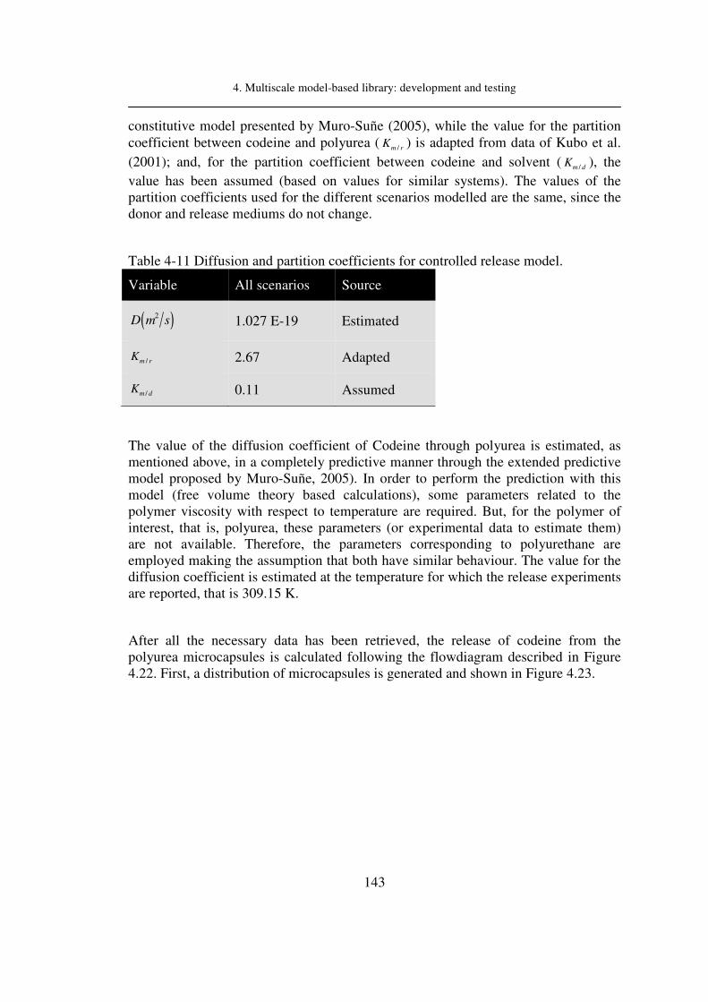
4. Multiscale model-based library: development and testing
143
constitutive model presented by Muro-Suñe (2005), while the value for the partition coefficient between codeine and polyurea ( /m rK ) is adapted from data of Kubo et al.
(2001); and, for the partition coefficient between codeine and solvent ( /m dK ), the
value has been assumed (based on values for similar systems). The values of the partition coefficients used for the different scenarios modelled are the same, since the donor and release mediums do not change.
Table 4-11 Diffusion and partition coefficients for controlled release model.
Variable All scenarios Source
( )2D m s 1.027 E-19 Estimated
/m rK 2.67 Adapted
/m dK 0.11 Assumed
The value of the diffusion coefficient of Codeine through polyurea is estimated, as mentioned above, in a completely predictive manner through the extended predictive model proposed by Muro-Suñe, 2005). In order to perform the prediction with this model (free volume theory based calculations), some parameters related to the polymer viscosity with respect to temperature are required. But, for the polymer of interest, that is, polyurea, these parameters (or experimental data to estimate them) are not available. Therefore, the parameters corresponding to polyurethane are employed making the assumption that both have similar behaviour. The value for the diffusion coefficient is estimated at the temperature for which the release experiments are reported, that is 309.15 K.
After all the necessary data has been retrieved, the release of codeine from the polyurea microcapsules is calculated following the flowdiagram described in Figure 4.22. First, a distribution of microcapsules is generated and shown in Figure 4.23.

4. Multiscale model-based library: development and testing
144
0.0 5.0x10⁻⁸
1.0x10⁻⁷
1.5x10⁻⁷
2.0x10⁻⁷
2.5x10⁻⁷
3.0x10⁻⁷
3.5x10⁻⁷
0
2
4
6
8
10
12
14
% o
f m
icro
cap
sule
s
Microcapsule radius (m)
Figure 4.23 Normal distribution of microcapsules for controlled release of codeine
For the three scenarios illustrated in Figure 4.24 which compare experimental data with results obtained from simulation, the curves of the solution of the mathematical model show a good agreement with the experimental values. This confirms the predictive ability of the mathematical model as well as the applicability to a pharmaceutical product. It is also very important to mention that the employed model corresponds to the prediction of a first order system, since no time effects were found in this experimental data.
0.0 0.5 1.0 1.5 2.0 2.5 3.0 3.5 4.00
10
20
30
40
% R
elea
se
time (hr)
Prediction scenario 1
Exp data scenario 1
Prediction scenario 2
Exp data scenario 2
Prediction scenario 3
Exp data scenario 3
Figure 4.24 Comparison between the experimental values and model predictions of the release of codeine.

4. Multiscale model-based library: development and testing
145
The multiscale modelling structure highlighted in these examples, is of the type, serial: transformation from nano-level (diffusion through the microcapsule wall) to the micro-scale (microcapsule) and simultaneous integration between micro-scale and macro-scale.
Controlled release of insecticide
This case study concerns the simulation of the controlled release of Permethrin [CAS number 52645-53-1] that is commonly employed to prevent attacks of insects in agricultural fields. The controlled release of the insecticide though the use of encapsulation can help to reduce the toxicity and also extend the biological effectivity of the active ingredient. Poly(butyl-methacrylate) (PBMA) is a possible polymer candidate for the microcapsule.
The size-parameters for the microcapsules have been taken from Muro-Suñe (2005), who adapted the data from Takahashi et al. (2006): diameter = 3.58 mµ ; thickness =
0.25-2.30 mµ ; and mean diameter = 0.3-46 mµ .
The objective here is to verify whether it is possible to get a release of 90% of Permethrin in 10 hours, considering the release to be of first order behaviour. Here, n-hexane has been suggested (Muro-Suñe, 2005) as donor solvent and water as the receiver medium. The remaining data necessary to perform the analysis is given in Table 4-12 and Table 4-13.

4. Multiscale model-based library: development and testing
146
Table 4-12 Permethrin microcapsule information.
Compound (2) Function Solubility of Permethrin in the compound (ppm)
Solubility of Permethrin in the compound (w1)
n-hexane Core solvent 106 0.5
Water Release Medium 0.006 6.0E-09
Table 4-13 Microcapsule characteristics.
Microcapsule properties m
Shell Thickness 0.537E-06 (Based on Takahashi et al., 2006)
Maximum radius 23E-06
Minimum radius 0.15E-06
Mean radius 1.79E-06
Standard deviation 1E-06
Radius step 0.1E-06
General information
Donor Value (3
m ) 7.88E-07
Receiver Vol. (3
m ) 0.0004
Time ( s ) 43200
Initial Concentration (3gr m ) 220825
Temperature ( K ) 313
As far as partition coefficient calculations are concerned, the calculation of infinite dilute activity coefficients for the permethrin-polymer, permethrin-donor and permethrin-receiver are needed. Permethrin-polymer calculations are carried out with the extended GC-Flory model (Muro-Suñé et al. 2005). This is a special model to predict the infinite dilute activity coefficients when a polymer is present. With respect to the calculation of the infinite dilute activity coefficients for the permethrin and the donor and the receiver, experimental data reported by Worthing (1979) has been used. When experimental data is not available, a predictive group contribution based model such as the UNIFAC model and its extension, the UNIFAC-CI model (Fredenslund,
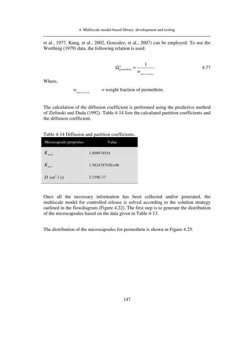
4. Multiscale model-based library: development and testing
147
et al., 1977, Kang, et al., 2002, Gonzalez, et al., 2007) can be employed. To use the Worthing (1979) data, the following relation is used:
/
1
donor receiver
permethrinw
∞Ω = 4.77
Where,
/donor receiver
w = weight fraction of permethrin.
The calculation of the diffusion coefficient is performed using the predictive method of Zielinski and Duda (1992). Table 4-14 lists the calculated partition coefficients and the diffusion coefficient.
Table 4-14 Diffusion and partition coefficients.
Microcapsule properties Value
/m dK 1.898974554
/m rK 1.582478795E+08
2 ( / )D m s 2.159E-17
Once all the necessary information has been collected and/or generated, the multiscale model for controlled release is solved according to the solution strategy outlined in the flowdiagram (Figure 4.22). The first step is to generate the distribution of the microcapsules based on the data given in Table 4-13.
The distribution of the microcapsules for permethrin is shown in Figure 4.25.

4. Multiscale model-based library: development and testing
148
0.0 2.0µ 4.0µ 6.0µ 8.0µ 10.0µ 12.0µ
0.0
0.5
1.0
1.5
2.0
2.5
3.0
3.5
4.0
4.5
% o
f m
icro
cap
sule
s
Microcapsule radius (m)
Figure 4.25 Distribution of microcapsules for controlled release of permethrin.
Figure 4.26 shows the simulated controlled release of permethrin from microcapsules made of PBMA polymer. The main goal of this example was to investigate whether it would be possible to get at least a 90% of release of permethrin in ten hours. According to the plot in Figure 4.26, it can be seen that this goal can be achieved. It is important to highlight that the model can also be used to study the behaviour of the release of permethrin as a function of the microcapsule size parameters.

4. Multiscale model-based library: development and testing
149
0 1 2 3 4 5 6 7 8 9 10 11 12 130
10
20
30
40
50
60
70
80
90
100
% R
elea
se
time (hr)
Figure 4.26 Profile of controlled release of Permethrin.
In general both examples show the flexibility and adaptability of the mathematical model for two different types of applications (pharmaceutical and agrochemical products). The first example shows the comparison and evaluation of the mathematical model, where experimental values for controlled release of codeine were available for comparison, and the second example highlights the use of the mathematical model for microcapsule design with desired (target) performance.


5. Application of the Virtual Product-Process Design Lab
151
5. Application of the Virtual Product-
Process Design Lab
In this chapter, three case studies related to the design of direct methanol fuel cell, a microcapsule for
controlled release of active ingredients; and pesticide uptake, are illustrated. All the case studies are
solved through the use of the Virtual product-process design lab (VPPD-l).
5.1. Direct Methanol Fuel Cell The design problem for the direct methanol fuel cell (DMFC) is based on the description of the device given in section 4.2. This example is illustrating the use of the reverse approach to generate a new alternative design of the energy production device. This example illustrates the versatility of the program to allow the user to apply the reverse approach through the use of the VPPD-l (Virtual Product-Process Design Lab).
5.1.1. VPPD-l layout: Direct methanol fuel cell
First, the layout for the direct methanol fuel cell template (interface) is retrieved in the VPPD-l, as shown in Figure 5.1, where the steps used to solve this problem are highlighted with a flag. The selection and use of the different options in the layout follow a clock-wise order.

5. Application of the Virtual Product-Process Design Lab
152
Fig
ure
5.1
Wo
rk-f
low
& d
ata-
flo
w i
n t
he
VP
PD
-l:
Dir
ect
met
han
ol
fuel
cel
l

5. Application of the Virtual Product-Process Design Lab
153
5.1.2. Redesign of a direct methanol fuel cell
The new hypothetical design of the DMFC is aimed to obtain the same value of the cell voltage (Ucell) (I), but with a new membrane design (d) where the diffusivity coefficients of protons and methanol ( θ ) in the membrane should be 15% lower than
the known (current) value. This is a difficult problem because of the likely incompatibility of the materials in the fuel cell. An alternative is to find out a temperature (Pt) which allows getting the same value of the cell voltage at the steady state with new values of diffusion coefficients. The problem-challenge statement highlights the possibility to apply the reverse approach using the VPPD-l, where ICAS-MoT is the modelling tool solving the model equations for the process variables (X). Here, (X) is used to get the value of the temperature condition through the solution of the differential algebraic set of equations (Table 4-5) so as to obtain the specified performance of the DMFC.
5.1.3. VPPD-l: direct methanol fuel cell
When the “Fuel cell” option is selected in the main menu of the VPPD-l (Figure 3.11), the corresponding interface on the virtual lab comes up, as illustrated in Figure 5.2. This interface has the characteristics described in section 3.2.1 (page 37) related to the requirements of multiscale modelling within a product-process design framework. The steps in the redesign of the direct methanol fuel cell are the following:
• Documentation about the product-process design
• Selection of the catalyst anode and cathode
• Introduction of membrane information
• Product-process behaviour modelling
Documentation about the product-process design
The first option is related with documentation about the design of the new product that is desired. In this example, we could specify the requirements in the new design of the fuel cell as well as the reasons for performing this change in the configuration of the DMFC structure. When the option is chosen, the program shows a window where it is possible to access the information later. This information is transferred to a text editor format (Microsoft Word, 2003), an option that is illustrated in Figure 5.3.

5. Application of the Virtual Product-Process Design Lab
154
Fig
ure
5.2
VP
PD
-l:
Dir
ect
met
han
ol
fuel
cel
l

5. Application of the Virtual Product-Process Design Lab
155
Figure 5.3 DMFC: Documentation about the product-process design.
Selection of the catalyst Anode and cathode
The next step is the selection of the anode and cathode catalyst type to be used in the device configuration (shown in Figure 5.4). The selection of this new fuel cell is Pt:Ru:C=25:25:50 (Platinum, Ruthenium and Carbon, respectively) on the anode, while Pt:C=50:50 (Platinum and Carbon, respectively) on the cathode.

5. Application of the Virtual Product-Process Design Lab
156
Figure 5.4 DMFC: Selection of cathode and anode type.
Introduction of membrane information
For the new configuration of the fuel cell, the target diffusivity coefficients of protons and methanol in the membrane should be 15% smaller than the currently used value
( 094.59M
HD e+
−= , 3
102.46M
CH OHD e−= ). The software has the option to introduce these
values manually (shown in Figure 5.5).

5. Application of the Virtual Product-Process Design Lab
157
Figure 5.5 DMFC: membrane information.
Product-process modelling behaviour
Simulation of the fuel cell behaviour is performed using the resident models available in the model library (shown in Figure 5.6).

5. Application of the Virtual Product-Process Design Lab
158
Figure 5.6 DMFC: Product-process modelling behaviour.
Behaviour of the new DMFC design is shown in Figure 5.7, where it is possible to observe that the value of the voltage for the new design is approximately the same (0.64042 V), as well as the values of the outlet concentration of (a) methanol (493.7059 mol/m3) and (b) carbon dioxide (2.7008 E-07 mol/m3). The results confirm that the redesign of the process device (obtained through the VPPD-l) is actually able to find the new temperature (352.071 K) for the new operation of the device. A higher temperature corresponding to the performance of the direct methanol fuel cell under the new configuration (that is, with improved values of diffusion coefficients) sounds logical as the lower diffusivity coefficients should increase the amount of energy supplied to the direct methanol fuel cell.

5. Application of the Virtual Product-Process Design Lab
159
Figure 5.7 Results of the new redesign of the DMFC.
At this point, the redesign of the DMFC in terms of the new material and process behaviour to achieve the desired target has been solved (Part I). The next part of the reverse approach is to find the new material with the desired properties that match the
0 500 1000 1500 2000 2500 3000 3500 40000.00004860.00004870.00004880.00004890.00004900.00004910.00004920.00004930.00004940.00004950.00004960.00004970.00004980.00004990.00005000.0000501
(a)
CC
H3O
H , m
ol/
m3
Time, s
SS
MS
0 500 1000 1500 2000 2500 3000 3500 40000.00E+000
5.00E-008
1.00E-007
1.50E-007
2.00E-007
2.50E-007
3.00E-007
(b)
CC
O2
, m
ol/
m3
Time, s
SS
MS
0 500 1000 1500 2000 2500 3000 3500 4000
0.6
0.7
0.8
0.9
1.0
1.1
1.2
Cell
Vo
lta
ge
(V)
Time, s
5. Application of the Virtual Product-Process Design Lab
160
target diffusion coefficient values for the methanol and the protons in a polymeric membrane. This search might be performed via molecular simulation, property prediction packages, or literature search, but has not been performed in this case study.
5.2. Uptake of pesticides from water droplets to
leaves
The development of agrochemical based products has become an important topic of collaborative research among the chemical engineering and life science communities. Usually, the designs of these products are performed thought the use of experiments. The application of mathematical modelling is an alternative that can be useful for virtual design of these products because it might provide tentative formulations (feasible candidates) that match the desired (targets) product qualities in a fast, efficient and inexpensive manner.
This example highlights the following features of the VPPD-l: the importance of the availability of an appropriate model-based library, database with different ingredients for the final formulation of the product and a demonstration of how the VPPD-l can be used to employ the forward approach for the design of a chemical based product.
5.2.1. Pesticide uptake model representation
Multiscale modelling analysis
This section describes the multiscale model analysis for the uptake of pesticides and highlights the importance of the use of models at the different scales. Figure 5.8 shows the scale-map of models used for pesticide uptake, where the modelling can be carried out in an entire field that basically corresponds to the macro-scale where the behaviour in a specific area is analyzed, and/or the impact of the pesticide on the environment is calculated. An analysis in the droplet scale can also be performed, that is, the behaviour of the active ingredient inside the droplet as well as the vaporization of the liquid phase are predicted (this plays an important role in pesticide uptake). Further analysis in a smaller scale (the behaviour of the pesticide uptake inside the leaf can also be predicted) can also be performed. Here, the importance of the pesticide mass transfer phenomenon between the droplet and the leaf as well as inside the leaf is considered, plus the pesticide concentration at the different layers inside the leaf is smaller.

5. Application of the Virtual Product-Process Design Lab
161
Figure 5.8 Scale-map for pesticide uptake.
Model-based library for uptake of pesticides
This application of the VPPD-l contains a model-based library that was earlier developed by Rasmussen (2004). Figure 5.9 illustrates the scheme of the mathematical model for the uptake of the pesticide into the leaf. The main parts that are considered in the mathematical model are: droplet, wax layer and cuticle layer.

5. Application of the Virtual Product-Process Design Lab
162
Figure 5.9 Pesticide uptake description at the different layers in the leaf (Rasmussen, 2004).
Mathematical models available in the model-based library have different characteristics, allowing the user to consider different types of phenomena when the product design pesticide formulation in these is performed. Table 5-1 lists the main characteristic of the different models.

5. Application of the Virtual Product-Process Design Lab
163
Table 5-1 Mathematical model description of the model-based library.
Mathematical Model Model Description
Model A Considers the cuticle and wax layer as one layer. The amount of solid pesticide is infinite. The concentration of the pesticide in the leaf is assumed constant over the time
Model B1 Considers the cuticle and wax layer as one layer. The amount of solid pesticide is infinite. The calculation of the diffusion coefficient for the surfactant is taking into account the number of ethoxy groups present in the surfactant molecule
Model B2 Considers the cuticle and wax layer as one layer. This model calculates the diffusion of the pesticide as well as the surfactant through the cuticle
Model C The droplet is the donor compartment. The cuticle layer acts as a receiver compartment for the pesticide and surfactant. The plant works as receiver compartment of the cuticle layer. The cuticle layer is divided in 100 layers
Model D The water evaporation rate is incorporated in the differential equations for the droplet. Diffusion coefficients for pesticide and surfactant should be supplied as known data and they are considered constant during the calculations
Model E The water evaporation rate is incorporated in the differential equations for the droplet. Diffusion coefficients for pesticide and surfactant are calculated in order to take into account the surfactant influence
5.2.2. VPPD-l layout: Uptake of pesticides
The VPPD-l layout for pesticide uptake is illustrated in Figure 5.10, which shows the different programs and options available in the “Pesticide uptake” template. The figure also provides a visual picture of the mathematical models available in the model-based library, and the sequence in which they are used together with the available options.

5. Application of the Virtual Product-Process Design Lab
164
Fig
ure
5.1
0 W
ork
-flo
w &
dat
a-fl
ow
in
th
e V
PP
D-l
: P
esti
cid
e U
pta
ke
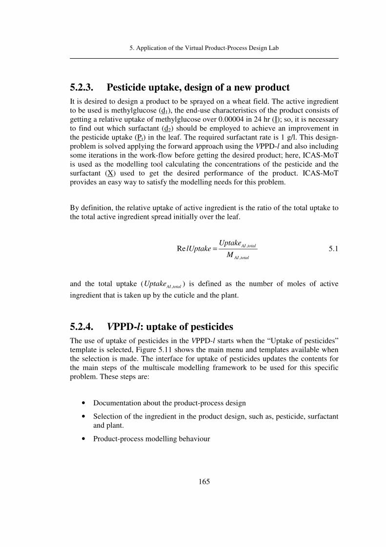
5. Application of the Virtual Product-Process Design Lab
165
5.2.3. Pesticide uptake, design of a new product
It is desired to design a product to be sprayed on a wheat field. The active ingredient to be used is methylglucose (d1), the end-use characteristics of the product consists of getting a relative uptake of methylglucose over 0.00004 in 24 hr (I); so, it is necessary to find out which surfactant (d2) should be employed to achieve an improvement in the pesticide uptake (Pt) in the leaf. The required surfactant rate is 1 g/l. This design-problem is solved applying the forward approach using the VPPD-l and also including some iterations in the work-flow before getting the desired product; here, ICAS-MoT is used as the modelling tool calculating the concentrations of the pesticide and the surfactant (X) used to get the desired performance of the product. ICAS-MoT provides an easy way to satisfy the modelling needs for this problem.
By definition, the relative uptake of active ingredient is the ratio of the total uptake to the total active ingredient spread initially over the leaf.
,
,
ReAI total
AI total
UptakelUptake
M= 5.1
and the total uptake ( ,AI totalUptake ) is defined as the number of moles of active
ingredient that is taken up by the cuticle and the plant.
5.2.4. VPPD-l: uptake of pesticides
The use of uptake of pesticides in the VPPD-l starts when the “Uptake of pesticides” template is selected, Figure 5.11 shows the main menu and templates available when the selection is made. The interface for uptake of pesticides updates the contents for the main steps of the multiscale modelling framework to be used for this specific problem. These steps are:
• Documentation about the product-process design
• Selection of the ingredient in the product design, such as, pesticide, surfactant and plant.
• Product-process modelling behaviour

5. Application of the Virtual Product-Process Design Lab
166
Fig
ure
5.1
1 V
PP
D-l
: U
pta
ke
of
Pes
tici
des

5. Application of the Virtual Product-Process Design Lab
167
Documentation about the product-process design
The first part is related with documentation of the new product design problem, which is common for all the available templates in the VPPD-l. When this option is chosen, the program shows a window where the user introduces the information which is transferred to a text editor format (Microsoft Word, 2003) as shown in Figure 5.3.
Selection of the ingredients in the product design: plant,
pesticide, surfactant.
This design-problem serves to highlight the need for a database with relevant information related to the ingredients to be used in the design. The selection of the plant (wheat) and the pesticide (methylglucose) is fixed for this example, but it is necessary to test which surfactant available in the database can be used in the pesticide formulation to increase the uptake. Therefore, some iteration might be required in the design of the product. Figure 5.12 shows the menu where the user is able to carry out the selection of the desired ingredients.
Figure 5.12 Pesticide uptake: Selection of the ingredients in the product design part.
5. Application of the Virtual Product-Process Design Lab
168
Once, the selection of the plant where the water droplets with the pesticide formulation is to be sprayed has been done, the first test starts with the trial and error selection of the surfactants available in the database.
Product-process modelling behaviour
After the selection of the surfactant, the selection of the “Perform product behaviour (Pesticide uptake)” option is used and a new interface opens, where the selection of the model that needs to be used is made, as shown in Figure 5.13. When the user selects a model from the model library, the program provides the description and assumptions (as shown in Table 5-1) associated with the model that the user has selected. This is followed by a series of “menus” that appear, and, where it is possible to verify the information as well as edit in case additional details are necessary. The information that can be edited is related to the general uptake problem, characteristics of the plant, active ingredient and surfactant. Subsequently, the option to “run:” the model is selected and the simulation results are retrieved and the option to plot the important variables is offered.

5. Application of the Virtual Product-Process Design Lab
169
Figure 5.13 Pesticide uptake: Product behaviour part.
This specific pesticide formulation design problem requires some trials to find the best surfactant to add from the database. The software enables this requirement so that different surfactants can be tested to find the one giving the best product performance (in this case, largest uptake in a specific time period). Table 5-2 shows

5. Application of the Virtual Product-Process Design Lab
170
the relative uptake of methylglucose for the different surfactants tested in the effort of obtaining the adequate surfactant.
Table 5-2 Relative uptake of methylglucose.
Surfactant Relative uptake of methylglucose
C13E11 4.66E-05
C13E15 2.31E-05
C13E20 1.31E-05
Figure 5.14 shows the plots of the relative uptake of methylglucose using different surfactants in the product composition.
Based on the results given in Table 5-2 or the plots in Figure 5.14, it can be clearly noted that the surfactant matching the desired (target) product characteristics is C13E11, because it provides the largest relative uptake of methylglucose at any specific time.
Figure 5.14 Pesticide uptake: Plots for the relative uptake of methylglucose.
0 5 10 15 200.00000
0.00001
0.00002
0.00003
0.00004
0.00005
Rel
ativ
e U
pta
ke
of
the
AI
Time, hr
C13E11
C13E15
C13E20

5. Application of the Virtual Product-Process Design Lab
171
Through this example, the capability of the VPPD-l to carry out the development of a new product with desired end-use characteristics is very nicely demonstrated for the specific case of the design of a pesticide formulation with the best possible uptake in a plant.
5.3. Microcapsule controlled release of active
ingredients The design-problem to be highlighted in this application example of the VPPD-l is the same as the example presented in section 4.3.5, but the difference, here is that the design problem is now solved with the software developed in this PhD-thesis.
This example highlights the integration of different computational-aided tools developed for the solution of product design problems concerning microcapsules for controlled release of active ingredients. Also, the structure of the framework and the way the work-flow and data-flow are employed to solve the problem, are highlighted. This problem also demonstrates the use of the VPPD-l with the aim of designing a product with desired end-use characteristics.
5.3.1. VPPD-l layout: Controlled release of active
ingredients
Figure 5.15 shows the VPPD-l layout with the template for the work-flow and data-flow for design of microcapsules for controlled release. This figure illustrates the different options available for the microcapsule controlled release template in the VPPD-l, where four main options are available that correspond to the main steps of the multiscale modelling framework for chemical product-process design. To solve the problem presented above, the options used are highlighted with a flag in the diagram.

5. Application of the Virtual Product-Process Design Lab
172
Fig
ure
5.1
5 W
ork
-flo
w &
dat
a-fl
ow
in
th
e V
PP
D-l
: M
icro
cap
sule
co
ntr
oll
ed r
elea
se o
f ac
tiv
e in
gre
die
nts

5. Application of the Virtual Product-Process Design Lab
173
5.3.2. Design of microcapsules for controlled release
The design problem consists of the design of microcapsules to be employed as protection against the attack of insects in wooden surfaces and/or fields. So, a controlled release of the active ingredient is required in order to reduce the toxicity of the product as well as to keep a longer biological effectivity of the active ingredient. The microcapsules encapsulate Permethrin which is the active ingredient. Water is the release medium, hexane is used as a solvent to dissolve the permethrin, is also used within the microcapsule. Finally, Poly(butyl-methacrylate) (PBMA), and is the polymer to be used in the microcapsule wall (d, < θ ). The aim of the design problem
is to check whether it is possible, to achieve a 90% of the release of permethrin in 10 hours (Pt), assuming the release profile to have a first order behaviour. All the required data/information for the problem is given in section 4.3.5, page 139.
5.3.3. VPPD-l: microcapsule controlled release of
permethrin
Figure 5.16 shows the screenshot when the “Controlled release” template is chosen in the VPPD-l. The main steps in the design for the microcapsules controlled release are:
• Documentation about the product-process design
• Selection of the active ingredient and polymer membrane
• Calculation of the diffusivity coefficient (Active ingredient-membrane)
• Calculation of partition coefficient
• Activity coefficients at infinite dilution and solubility of active ingredients in the solvent and release medium.
• Calculation of partition coefficient between the active ingredient and the polymer membrane wall.
• Product-process modelling behaviour
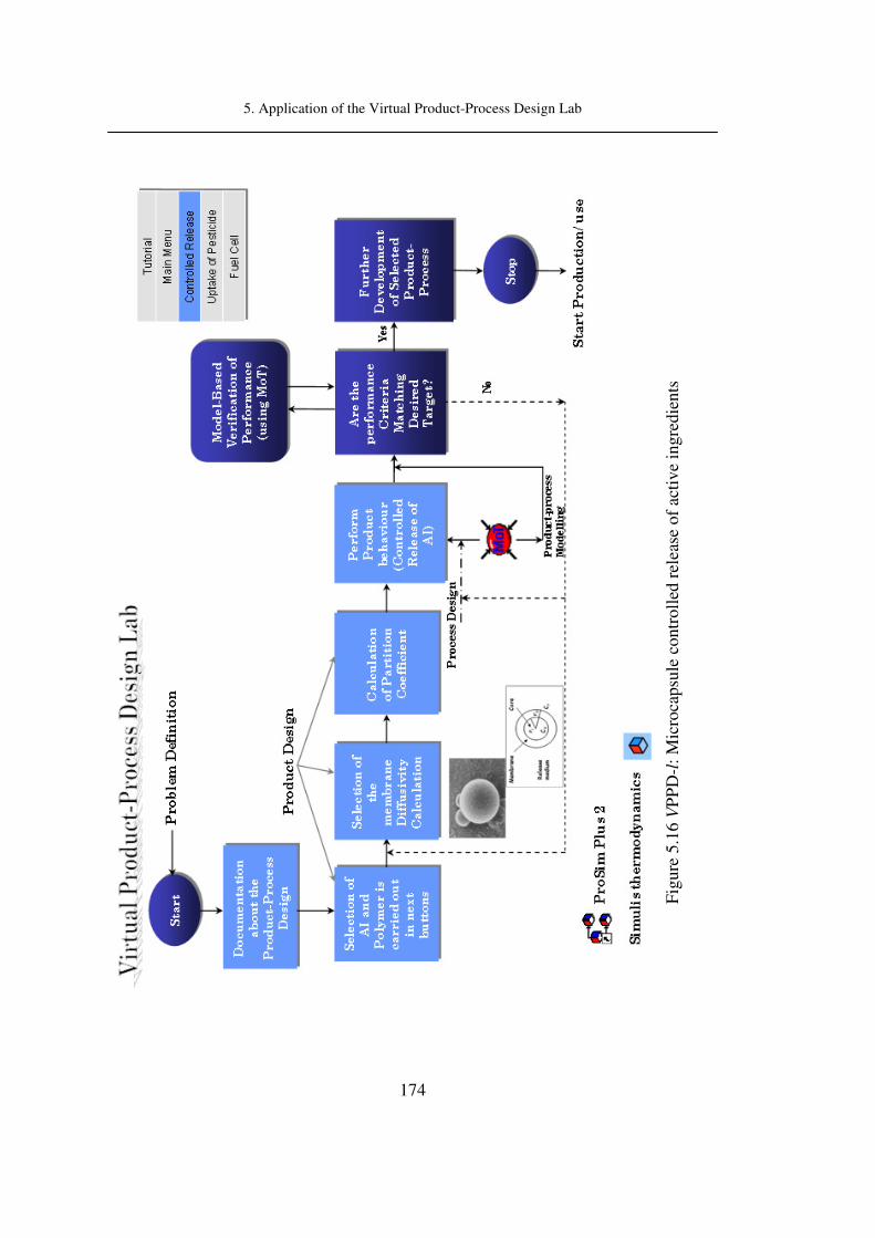
5. Application of the Virtual Product-Process Design Lab
174
Fig
ure
5.1
6 V
PP
D-l
: M
icro
cap
sule
co
ntr
oll
ed r
elea
se o
f ac
tiv
e in
gre
die
nts

5. Application of the Virtual Product-Process Design Lab
175
Documentation about the product-process design
The process of systematic design for the desired product starts with the documentation and assumptions about the product (see Figure 5.17).
Figure 5.17 Microcapsule for controlled release: Documentation about the product-process design.
Selection of the active ingredient and membrane
In the next step, the selection of the membrane polymer is made as well as the active ingredient needed for the formulation, as shown in Figure 5.18, in this case, PBMA and permethrin, respectively are selected.

5. Application of the Virtual Product-Process Design Lab
176
Figure 5.18 Microcapsule for controlled release: Selection of the polymer membrane and active ingredient.
Calculation of the diffusivity coefficient (Active ingredient-
membrane)
The selection of active ingredients and membrane also involves the calculation of the diffusion coefficients of the active ingredient through the membrane polymer wall. To perform this calculation, an external interface containing the extension of the Zielinski and Duda, (1992) model (based on group contribution method) proposed by Muro Suñé (2005), for the prediction of compound property is called (see Figure 5.19). This interface also calls other programs related with the calculation of properties of the compounds used in the formulated product. For example: the calculations of some properties (such as, critical volume, molecular weight, glass temperature, etc.) are carried out using the ProPred package in ICAS. On the other hand, the database manager may be used to search the properties in a database collection, or even to obtain information about some correlations used to calculate the specific volume in a required temperature range. The Icassim environment can be employed to perform also the calculation of specific volume or to perform viscosity calculations, and all the software mentioned above for property predictions is
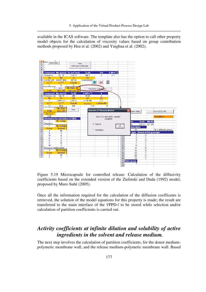
5. Application of the Virtual Product-Process Design Lab
177
available in the ICAS software. The template also has the option to call other property model objects for the calculation of viscosity values based on group contribution methods proposed by Hsu et al. (2002) and Yinghua et al. (2002).
Figure 5.19 Microcapsule for controlled release: Calculation of the diffusivity coefficients based on the extended version of the Zielinski and Duda (1992) model, proposed by Muro Suñé (2005).
Once all the information required for the calculation of the diffusion coefficents is retrieved, the solution of the model equations for this property is made; the result are transferred to the main interface of the VPPD-l to be stored while selection and/or calculation of partition coefficients is carried out.
Activity coefficients at infinite dilution and solubility of active
ingredients in the solvent and release medium.
The next step involves the calculation of partition coefficients, for the donor medium-polymeric membrane wall, and the release medium-polymeric membrane wall. Based

5. Application of the Virtual Product-Process Design Lab
178
on the available information on the calculation of the partition coefficients, first, the calculation of the infinite dilution activity coefficient for the permethrin – n-hexane and permethrin – water, is performed using experimental solubility data of the active ingredient with each of the mediums. This is illustrated in Figure 5.20. If experimental data is available, it can be used, otherwise, a predictive model such as the UNIFAC model and extensions as UNIFAC-CI (Fredenslund et al., 1977, Kang et al., 2002, Gonzalez et al., 2007) can be employed. In this case, it is possible to calculate infinite dilute activity using the model proposed by Worthing (1979), which is available within the property model library for the design template.
Figure 5.20 Microcapsule for controlled release: Introduction of activity coefficients at infinite dilution and solubility of active ingredients in the solvent and release medium.

5. Application of the Virtual Product-Process Design Lab
179
Calculation of partition coefficient between the active
ingredient and the polymer membrane wall.
For the calculation of the permethrin-PBMA activity coefficient, an extension of the GC-Flory model (Muro-Suñé et al. 2005) that is a special model to predict the infinite dilute activity coefficients (when a polymer is present), is employed. When the “GC-Flory” option is chosen, a new interface opens in order to carry out the necessary calculations. Figure 5.21 illustrates the interface, where the method to compute the property based on the group contribution method is employed. Once the activity coefficient is computed, this information is transferred to the VPPD-l.
Figure 5.21 Microcapsule for controlled release: Calculation of partition coefficient between the active ingredient and the polymer membrane wall (Muro-Suñé, et al. 2005).
Product-process modelling behaviour
Once all the necessary data and information has been retrieved, “Perform product behaviour (Controlled Release of AI)” is selected, and all collected information and/or calculated information (such as, diffusion coefficient, partition coefficient, chemical compounds, etc.) are passed to the current “menu” (interface). Here first, the information obtained from the main interface (VPPD-l) is loaded automatically (as shown in Figure 5.22), and the verification of this information is made. It is also possible to edit the information, if necessary.

5. Application of the Virtual Product-Process Design Lab
180
Figure 5.22 Microcapsule for controlled release: Modelling data.
Simulation results from the solution of the controlled release model are shown in Figure 5.23. Given the input data (I) and geometry chosen for the microcapsule, it is possible to observe that the target criterion has been matched, that is, the 90% release from the capsule has been achieved in 10 hours, as specified in the product description.

5. Application of the Virtual Product-Process Design Lab
181
Figure 5.23 Microcapsule controlled release: controlled release behaviour of permethrin.
This case study highlights the advantages of the VPPD-l, in terms of software architecture (handle the needs of different model interfaces), data-flow, reliable use of the VPPD-l in the design of new products, and finally, the design steps (work-flow) to achieve the end-use property targets. Even though the example is solved by the forward approach, the VPPD-l can also manage the reverse approach for this type of design problems. One case might be the design of microcapsules where given one active ingredient, the donor and the release medium, it is desired to develop a product having specific release behaviour consisting of: 10% of active ingredient release in 3 hours (as lower limit) and 50% of active ingredient release in 1 hours (as upper limit), as shown in Figure 5.24. The active ingredient to be released is known in advance with the exception of the identity of the polymeric membrane. The design problem, therefore, concerns the finding of the polymeric material able to achieve the target behaviour.
Thus, given the product targets, product performance behaviour is predicted in order to find the appropriate property values, which will define the potential materials used for the final conformation of the product. The final decision about the product is made after a literature search, and use of group contribution methods, etc. is carried out to find the missing polymeric membrane details.
0 1 2 3 4 5 6 7 8 9 10 11 12 130
10
20
30
40
50
60
70
80
90
100
% R
ele
ase
time (hr)

5. Application of the Virtual Product-Process Design Lab
182
Figure 5.24 Microcapsule controlled release: reverse approach application.
5.4. CAPE-OPEN Standards: Software
integration. The use of CAPE-OPEN standards has been highlighted above with three different case studies involving the interaction between ICAS-MoT and Simulis thermodynamics®, ProSimPlus 2 and COFE. The link to access to this interaction is shown on the bottom part of the VPPD-l interface (see Figure 5.2, Figure 5.11 or Figure 5.16) where a direct connection to the external (simulators and property prediction) programs is carried out. More details about these case studies are illustrated in section 3.5.3.
0 1 2 3 4 50
20
40
60
80
100
% R
ele
ase
Time, hr
Lower boundary
Upper boundary

6. Conclusion
183
6. Conclusion
6.1. Achievements
The main achievements of this PhD-project are the introduction of the generic multiscale modelling framework and its implementation into a software for chemical product-process design that allows the virtual development of products with desired end-use characteristics, which is supported by a systematic manner to solve product-process design problems. The problem solution consists of four main steps:
• Problem definition: conceptual definition of the design problem.
• Product design: generation of data/knowledge related to the product needs, and selection of the materials to be added to the product as well as the calculation of the necessary properties related simulation model.
• Product-process modelling: evaluation of the product performance through mathematical modelling.
• Product-process evaluation: test the product in a laboratory as a tentative final design and see between compatibility of the reality and the virtual design product.
The last steps have been highlighted through case studies related to the development of three different types of chemicals based products.

6. Conclusion
184
The application of the generic multiscale modelling framework has been shown with the development and adaptation of it in a computer-aided tool called the “Virtual
Product-Process Design Lab”, that basically involved the development of a software incorporating various computer-aided tools (most of them available in ICAS) that facilitates the solution of problems related to the design of chemical products through the use of systematic work-flow and data-flow for different types of chemical products.
For the development of the Virtual Product-Process Design Lab to be successful and reliable, an integration of different tools was necessary. This was achieved with the aim of providing the user, different sources of information concerning properties (transport, thermodynamics, etc.) that are usually needed in the solution of the investigated product design problems. The virtual lab has a link with a commercial simulator that enables it to have a connection with ICAS-MoT (modelling tool) through the use of CAPE-OPEN Standards. This is made possible through the creation of model objects (using ICAS-MoT) for a unit operation not available in the external simulator model library. Also property models not available in the library could be added in this way.
The use of the developed software is illustrated through three case studies: direct methanol fuel cell, microcapsule based controlled release of active ingredients and pesticide uptake. The case studies highlight the application of the design problem solution through the software in a systematic way, achieving the desired targets in the product. For example, the use of forward and reverse approaches for product design is highlighted. The use of the forward approach has been highlighted for problems related to pesticide uptake and microcapsule based controlled release of active ingredients, while the design of a direct methanol fuel cell has been found using the reverse approach where the characteristics of a membrane with the desired properties have been identified.
It is also very important to highlight the importance of the multiscale modelling and the management of the models and their implementation into a software in an efficient and flexible way for the solution/design of chemical products.
In general, the important milestones in this PhD-Thesis were:
• The development of a systematic multiscale model-based framework for product-process design and its application illustrated through the development of the Virtual Product process Design Lab. - achieved.

6. Conclusion
185
• The introduction of an alternative to the usual trial and error experimental-based approach, which allows some of the time consuming and repetitive steps to be performed virtually through a model-based framework. In this way, the resources of experimental work are reserved for the final verification of the product, when a small number of candidates matching the desired end-use characteristics of the product could be tested. - achieved.
• The development of an intelligent, flexible and efficient combination and integration of different modelling tools. - achieved.
• Use current software interface techniques to integrate different methods and tools. Consider the use of CAPE-OPEN standard interfaces to allow the designer to create customized process and property calculations involving multiscale modelling. - achieved.
• Development of special process models not found in model libraries, for example, the Wiped film evaporator process-model needed by industry. Develop, implement and validate the model. – achieved.
6.2. Recommendation for future work This PhD-Thesis has shown the importance of the introduction of a multiscale modelling framework in product-process design, as well as its application through the development of the Virtual product-process design Lab, that contains a model-based library for three different chemical based products. In order to have a wider applicability of the developed software, it is necessary to add new mathematical models to the model-based library together with different representations of the model equations, for instance, different representations at different scales, different simplifications of mathematical models, model reduction techniques, model decomposition techniques and many more. It is also recommended to try to involve more computer-aided tools, such as design of formulated products and design of new process operations and/or devices.


7. Appendixes
187
7. Appendixes
7.1. Appendix 1: WFE Model
7.1.1. Introduction
The Wiped Film Evaporator model was designed to carry out the simulation for purification of one product in the aromatic industry. This Wiped Film Evaporator case study, also explains the COM (Component Object Module) generation feature of ICAS-MoT and how it can be used through Excel, in order to facilitate the way to handle and analyze the results given by the proposed mathematical model.
7.1.2. Wiped Film Evaporator Model
The developed generalized two-dimensional steady state model for the wiped film evaporator makes the following assumptions:
A1. The process is in steady state.
A2. The liquid films on the evaporation and condensation walls are much thinner than the corresponding cylinder diameters.
A3. Rectangular coordinates are used.
A4. The liquids are Newtonian.
A5. The flow in the vertical direction is laminar.
A6. Re-evaporation and splashing phenomena are neglected.

7. Appendixes
188
A7. Operation occurs far from the extremities of the evaporator (i.e. for a fully developed flow).
A8. There is no diffusion in the axial direction and the radial flow is neglected.
A9. Rotational phenomena are neglected in the model.
Momentum balance
In most cases of wiped film evaporator, the evaporating liquid is highly viscous and hence the corresponding Reynolds numbers are small. The Navier-Stokes equation (at steady state) for laminar flow regime describes the velocity profile of falling film:
( )( )2
2
,,
v y zv y z g
y
∂= −
∂ (7.1)
where, y and z are the radial and axial coordinates respectively, v is the velocity and g is the gravitational constant. Eq. (7.1) has the following boundary conditions
( ) ( ) max0, 0, ,v z v y z v= = (7.2)
Rate of evaporation
The rate of evaporation is obtained from the continuity equation in terms of flow rate
( l
iI ) for each component i in the liquid phase.
( )
( ) ,2 , 1, , ; 0l
i l l
i i i o
I zR k i N I I
zπ
∂= − ⋅ ⋅ = =
∂… (7.3)
where, the effective rate of evaporation of each component (ki) is calculated through a modified Langmuir-Knudsen equation.
( )
, 1, ,2
vap
i i
i
refg i s
p Pk i N
PR M T z
γ
π
= =
… (7.4)
Eq. (7.4) contains a factor (P/Pref) for correcting the vacuum pressure. The effective rate of evaporation [Eq. (7.4)] also depends on some mixture properties (activity
coefficient γi, vapour pressure pivap
and molecular weight Mi of each compound) as well as design parameters (the radius of the evaporator inside cylinder R and the surface temperature Ts).
As far as vapour phase concerns, the equation is similar to (7.3) with the only

7. Appendixes
189
difference that the sign in the right side is contrary because in this case, the amount of material lost for the liquid phase is gained for the vapour phase.
( )
( ) ,2 , 1, , ; 0v
i v v
i i i o
I zR k i N I I
zπ
∂= ⋅ ⋅ = =
∂… (7.5)
Energy balance
The temperature (T) profile in the falling film is given by the equation
( )( ) ( ) ( )2 2
2 2
, , ,,
T y z T y z T y zv y z
z Cp y z
λ
ρ
∂ ∂ ∂= +
∂ ∂ ∂ (7.6)
With boundary conditions at z = 0 (i.e. at the feed position the temperature corresponds to the liquid feed temperature), at y = 0 (i.e. at the evaporation surface, the temperature corresponds to the wall evaporation temperature) and y = h1 (i.e. the
heat flux from the liquid film surface is given by the evaporation heat ∆Hvap and the
effective net rate of evaporation k):
( ) ( )( )
1
1
,,0 , 0, , vap
F w
y h
T y zT y T T z T H k
yλ
=
∂= = = ∆ ⋅
∂ (7.7)
1
1
Ni i
Ni
kk
C kk
C=
=
=
∑∑
(7.8)
Where λ, ρ, Cp, ∆Hvap are the thermal conductivity, density, thermal capacity and
heat of evaporation of the multi-component mixture, respectively; and xi is the mole fraction of the i-th component.
i i
i
xλ λ=∑ 7.9
i i
i
xρ ρ=∑ 7.10
i i
i
Cp Cp x=∑ 7.11

7. Appendixes
190
vap vap
i i
i
H H x∆ = ∆∑ 7.12
Mass Balance
The composition (i
C ) profiles for each component are calculated from the diffusion
equation.
( )( ) ( ) ( )2 2
2 2
, , ,, , 1, ,i i i
i
C y z C y z C y zv y z D i N
z y z
∂ ∂ ∂= + =
∂ ∂ ∂ … 7.13
Where i
D is the (constant) diffusion coefficient for the thi component, and N is the
total number of components.
The boundary conditions for equation 7.13 are
( )( )
( )( )
1
,0
0,,0 , 0,
0,,
i
i i
i
i i z
y h
C zC y C
y
C zD I
y=
∂= =
∂∂
=∂
7.14
Mole fraction for each compound is calculated using:
ii
Cx
c= 7.15
Film thickness
Finally, an important variable of interest is the film thickness (h1) along the evaporator height that is calculated as follows
( ) ( )31
3
2h z I z
R g c
ν
π=
⋅ ⋅ ⋅ (7.16)
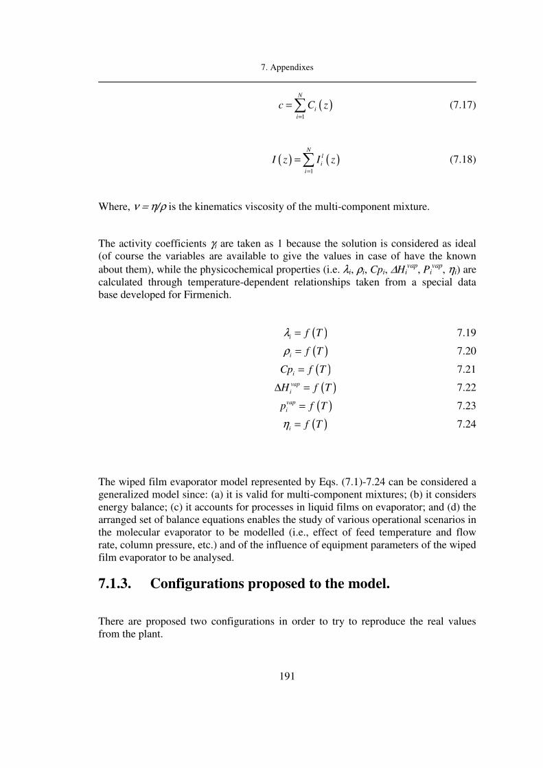
7. Appendixes
191
( )1
N
i
i
c C z=
=∑ (7.17)
( ) ( )1
Nl
i
i
I z I z=
=∑ (7.18)
Where, ν = η/ρ is the kinematics viscosity of the multi-component mixture.
The activity coefficients γi are taken as 1 because the solution is considered as ideal (of course the variables are available to give the values in case of have the known
about them), while the physicochemical properties (i.e. λi, ρi, Cpi, ∆Hivap, Pi
vap, ηi) are calculated through temperature-dependent relationships taken from a special data base developed for Firmenich.
( )i f Tλ = 7.19
( )i f Tρ = 7.20
( )iCp f T= 7.21
( )vap
iH f T∆ = 7.22
( )vap
ip f T= 7.23
( )i f Tη = 7.24
The wiped film evaporator model represented by Eqs. (7.1)-7.24 can be considered a generalized model since: (a) it is valid for multi-component mixtures; (b) it considers energy balance; (c) it accounts for processes in liquid films on evaporator; and (d) the arranged set of balance equations enables the study of various operational scenarios in the molecular evaporator to be modelled (i.e., effect of feed temperature and flow rate, column pressure, etc.) and of the influence of equipment parameters of the wiped film evaporator to be analysed.
7.1.3. Configurations proposed to the model.
There are proposed two configurations in order to try to reproduce the real values from the plant.

7. Appendixes
192
Single WFE configuration
First of all, it is proposed to use the simple model for the wiped film evaporator obtaining the result directly from the simulation of this set of equations. The configuration is shown following in Figure 7.1.
Figure 7.1 Single WFE configuration
Alternative configuration for WFE unit
On the other hand, it is proposed the combination of flash unit, WFE model and a simple mixer getting next configuration (see Figure 7.2).
Figure 7.2 Alternative representation for WFE unit
First, the mixture stream is fed to a flash unit to the conditions of pressure and temperature; it should be highlighted that the temperature for the vapour going out should be known. The liquid going out of the flash unit is feed to WFE unit and the vapour produced in this unit is mixed with the vapour from the flash unit.
Flash unit is able to handle to feed streams and physical equilibrium is calculated

7. Appendixes
193
using Peng-Robinson equation of state.
By the way, this is a very good example to highlight the advantage of use or more that one MoT model in the same Excel interface. Furthermore, this represents another option for the simulation of the wiped film evaporator unit.
7.1.4. Database for special compounds.
A special data base with the main physicochemical properties (i.e. λi, ρi, Cpi, ∆Hivap,
Pivap) has been developed. This data base was developed using a Component Property
prediction tool (ProPred) and “Data Base Manager” tool, both of them available in the ICAS software developed by Computer Aided Process-Product Engineering Center at the Technical University of Denmark.
7.1.5. Model Solution: computer-aided integration (ICAS-
MoT – Excel)
Software integration
Together with the development of the mathematical model for the wiped film evaporator, an integration between ICAS-MoT and Excel has been performed (shown in Figure 7.3). Here, Microsoft Excel is working as the user interface that requires the support of ICAS-MoT and it is connected through COM Objects.
Figure 7.3 ICAS-Mot – Excel integration software.
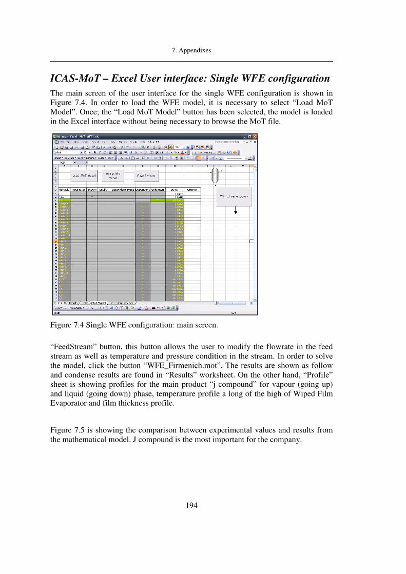
7. Appendixes
194
ICAS-MoT – Excel User interface: Single WFE configuration
The main screen of the user interface for the single WFE configuration is shown in Figure 7.4. In order to load the WFE model, it is necessary to select “Load MoT Model”. Once; the “Load MoT Model” button has been selected, the model is loaded in the Excel interface without being necessary to browse the MoT file.
Figure 7.4 Single WFE configuration: main screen.
“FeedStream” button, this button allows the user to modify the flowrate in the feed stream as well as temperature and pressure condition in the stream. In order to solve the model, click the button “WFE_Firmenich.mot”. The results are shown as follow and condense results are found in “Results” worksheet. On the other hand, “Profile” sheet is showing profiles for the main product “j compound” for vapour (going up) and liquid (going down) phase, temperature profile a long of the high of Wiped Film Evaporator and film thickness profile.
Figure 7.5 is showing the comparison between experimental values and results from the mathematical model. J compound is the most important for the company.

7. Appendixes
195
Figure 7.5 Comparison of the model with experimental values. Single WFE configuration.
0.0000
0.0100
0.0200
0.0300
0.0400
0.0500
0.0600
0.0700
0.0800
0.0900
0.1000
a b c d f g h i j k l m
Compound
Residue Stream
Experimental
Calculated
0.0000
0.1000
0.2000
0.3000
0.4000
0.5000
0.6000
0.7000
0.8000
0.9000
a b c d f g h i j k l m
Compound
Distillate Stream
Experimental
Calculated

7. Appendixes
196
ICAS-MoT – Excel User interface: Alternative representation
for WFE unit
This part corresponds to the second configuration (Flash unit, WFE and Mixer) and this was also improved due to the use of different model, the time used linking different models was long.
The interface is working describing the alternative representation for WFE unit (see Figure 7.6). An extra button is added to this interface “Update dependent variables information” that is explained below.
In order to load the WFE model it is necessary to push “Load MoT Model” “FeedStream” button also is available; this button allows the user to modify the flowrate in the feed stream as well as temperature and pressure condition in the stream.
Figure 7.6 Alternative representation of WFE unit: main screen.
In order to solve the WFE with this configuration (mentioned above); next steps should be carried out:

7. Appendixes
197
• Run flash unit (click on “Flash.mot” button).
• Run WFE unit (click on “WFE_Firmenich.mot” button).
• Click on “Update dependent variables information” button so as to keep this information available in the future.
• Last step is to click on “Mixer.mot”.
The results are shown as follow and condense results are found in “Results” worksheet. As it is mentioned in section, it is possible to see the profile for the main product “j product” for vapour (going up) and liquid (going down) phase, temperature profile a long of the high of Wiped Film Evaporator and film thickness profile. Those can be found in “Profile” sheet.
Figure 7.7 is showing the comparison between experimental values and results from the mathematical model. j compound is the most important for the company.

7. Appendixes
198
Figure 7.7 Comparison of the model with experimental values. Alternative representation of WFE unit.
If a comparison is carried out between two proposed configurations, it is possible to observe that single configuration has a better accuracy with respect to the experimental values.
0.0000
0.1000
0.2000
0.3000
0.4000
0.5000
0.6000
0.7000
0.8000
0.9000
a b c d f g h i j k l m
Compound
Distillate Stream
Experimental
Calculated
0.0000
0.0100
0.0200
0.0300
0.0400
0.0500
0.0600
0.0700
0.0800
0.0900
0.1000
a b c d f g h i j k l m
Compound
Residue Stream
Experimental
Calculated
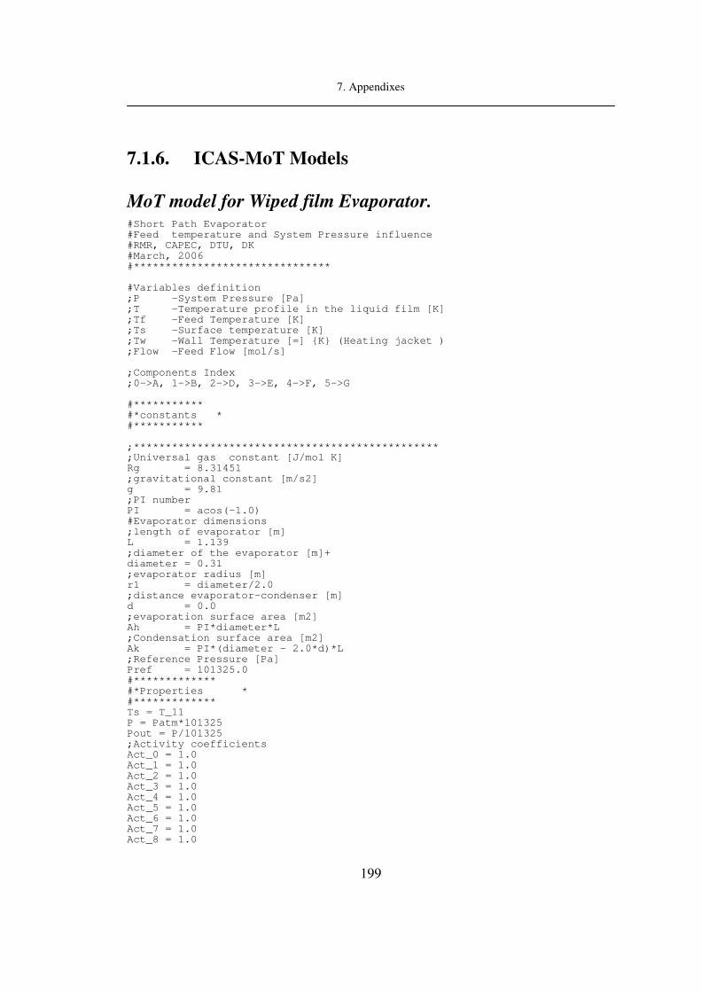
7. Appendixes
199
7.1.6. ICAS-MoT Models
MoT model for Wiped film Evaporator. #Short Path Evaporator #Feed temperature and System Pressure influence #RMR, CAPEC, DTU, DK #March, 2006 #******************************* #Variables definition ;P -System Pressure [Pa] ;T -Temperature profile in the liquid film [K] ;Tf -Feed Temperature [K] ;Ts -Surface temperature [K] ;Tw -Wall Temperature [=] K (Heating jacket ) ;Flow -Feed Flow [mol/s] ;Components Index ;0->A, 1->B, 2->D, 3->E, 4->F, 5->G #*********** #*constants * #*********** ;************************************************ ;Universal gas constant [J/mol K] Rg = 8.31451 ;gravitational constant [m/s2] g = 9.81 ;PI number PI = acos(-1.0) #Evaporator dimensions ;length of evaporator [m] L = 1.139 ;diameter of the evaporator [m]+ diameter = 0.31 ;evaporator radius [m] r1 = diameter/2.0 ;distance evaporator-condenser [m] d = 0.0 ;evaporation surface area [m2] Ah = PI*diameter*L ;Condensation surface area [m2] Ak = PI*(diameter - 2.0*d)*L ;Reference Pressure [Pa] Pref = 101325.0 #************* #*Properties * #************* Ts = T_11 P = Patm*101325 Pout = P/101325 ;Activity coefficients Act_0 = 1.0 Act_1 = 1.0 Act_2 = 1.0 Act_3 = 1.0 Act_4 = 1.0 Act_5 = 1.0 Act_6 = 1.0 Act_7 = 1.0 Act_8 = 1.0

7. Appendixes
200
Act_9 = 1.0 Act_10 = 1.0 Act_11 = 1.0 #Critical Temperature [K] ;Critical Temperature [K] Tc[i] = DB_Tc[i] #Boling point temperature [K] ;Boiling Temperature [K] Tb[i] = DB_Tb[i] #Molecular weight [g/grmol] MW[i] = DB_Mw[i] ;Molecular Weight[kg/mol] MW[i] = MW[i]/1000.0 #Reduced temperature Tr[i] = Ts/DB_Tc[i] #************************* #Liquid Density [kmol/m^3] #Dippr100 #A/B^(1 + (1 - Ts/C)^D) LiquidDensity[i] = (ADippr100[i]/BDippr100[i])^(1 -Ts/CDippr100[i])^DDippr100[i] #********************************************************************************* ;[kg/m3] rho[i] = LiquidDensity[i]*MW[i]*1000.0 #************************* #Vapour Pressure [Pa] #Dippr101 #exp(A + B/Ts + C*ln(Ts) + D*Ts^E) VapourPressure[i] = exp(ADippr101[i] + BDippr101[i]/ Ts + CDippr101[i]*ln(Ts) + DDippr101[i]*Ts^EDippr101[i]) #*********************************************************************************************************** ;Pressure of saturated vapor [Pa] Pvap[i] = VapourPressure[i] #***************************** #Heat of Vaporization [J/kmol] #Dippr102 #A*(1 - Tr)^(B + C*Tr + D*Tr^2) HeatVaporization[i] = ADippr102[i]*(1 - Tr[i])^(BDippr102[i] + CDippr102[i]*Tr[i] + DDippr102[i]*Tr[i]^2) #*********************************************************************************************************** ;[kJ/mol] DHvap[i] = HeatVaporization[i] /(1000.0*1000.0) #********************************** #Liquid Heat Capacity [J/(kmol*K)] ##Dippr103 #A + B*Ts + C*Ts^2 + D*Ts^3 + E*Ts^4 LiquidHeatCapacity[i] = ADippr103[i] + BDippr103[i]*Ts + CDippr103[i]*Ts^2 + DDippr103[i]*Ts^3 + EDippr103[i]*Ts^4 #*********************************************************************************************************** ;Liquid Heat Capacity [J/(mol*K)] Cp[i] = LiquidHeatCapacity[i] / 1000.0 Cp_0 = (ADippr103_0*(1 - Tr_0)^(BDippr103_0 + CDippr103_0*Tr_0 + DDippr103_0*Tr_0^2))/1000.0 #*************************** #Liquid Viscosity [kg/(m*s)] #Dippr104 #exp(A+B/Ts+C*ln(Ts)+D*Ts^E) LiquidViscosity[i] = exp(ADippr104[i] + BDippr104[i]/ Ts + CDippr104[i]*ln(Ts) + DDippr104[i]*Ts^EDippr104[i]) #*********************************************************************************************************** Eta[i] =LiquidViscosity[i] #*************************************** #Liquid Thermal Conductivity [J/(m*s*K)]

7. Appendixes
201
#Dippr105 #A + B*Ts + C*Ts^2 + D*Ts^3 + E*Ts^4 LiquidThermalCond[i] = ADippr105[i] + BDippr105[i]*Ts + CDippr105[i]*Ts^2 + DDippr105[i]*Ts^3 + EDippr105[i]*Ts^4 #*********************************************************************************************************** ;Thermal Conductivity [W/(m K)] Lambda[i] = LiquidThermalCond[i] ;Kinematic Viscosity [m2/s] nu[i] = Eta[i]/rho[i] ;Total concentration [mol/m3] Q[i] = Flow[i]*MW[i]/rho[i] Qtot = sum_i(Q[i]) C[i] = Flow[i]/Qtot Ctot = sum_i(C[i]) ;molar feed flow [mol/s] and [kmol/hr] FlowTot = sum_i(Flow[i]) FvTot = sum_i(Fv[i]) FlowkmTot = sum_i(Flowkm[i]) FvkmTot = sum_i(Fvkm[i]) ;Mixture properties x[i] = Flow[i]/FlowTot yv[i] = Fv[i]/FvTot rhoMix = sum_i(x[i]*rho[i]) LambdaMix = sum_i(x[i]*Lambda[i]) CpMix = sum_i(x[i]*Cp[i]) MWMix = sum_i(x[i]*MW[i]) EtaMix = sum_i(x[i]*Eta[i]) DHvapMix = sum_i(x[i]*DHvap[i]) nuMix = EtaMix/rhoMix #********************************************* EREF = 1.0 ;Pressure system effect EREF = EREF*(P/Pref) #********************************************** ;Integration parameter ;Number of radial integration points. N = 11 ay = 0.0 #********************************************** ;film thickness h1 = (3.0*nuMix*FlowTot/(2.0*PI*r1*g*Ctot))^(1.0/3.0) ;h1 = 0.000666 ;radial integration points by = h1 Dy = (by - ay)/N Y_1 = Dy Y_2 = 2.0*Dy Y_3 = 3.0*Dy Y_4 = 4.0*Dy Y_5 = 5.0*Dy Y_6 = 6.0*Dy Y_7 = 7.0*Dy Y_8 = 8.0*Dy Y_9 = 9.0*Dy Y_10 = 10.0*Dy ;velocity field Vz_1 = g*h1^2/nuMix*(Y_1/h1 - 0.5*Y_1*Y_1/h1^2) Vz_2 = g*h1^2/nuMix*(Y_2/h1 - 0.5*Y_2*Y_2/h1^2) Vz_3 = g*h1^2/nuMix*(Y_3/h1 - 0.5*Y_3*Y_3/h1^2) Vz_4 = g*h1^2/nuMix*(Y_4/h1 - 0.5*Y_4*Y_4/h1^2) Vz_5 = g*h1^2/nuMix*(Y_5/h1 - 0.5*Y_5*Y_5/h1^2) Vz_6 = g*h1^2/nuMix*(Y_6/h1 - 0.5*Y_6*Y_6/h1^2) Vz_7 = g*h1^2/nuMix*(Y_7/h1 - 0.5*Y_7*Y_7/h1^2) Vz_8 = g*h1^2/nuMix*(Y_8/h1 - 0.5*Y_8*Y_8/h1^2) Vz_9 = g*h1^2/nuMix*(Y_9/h1 - 0.5*Y_9*Y_9/h1^2) Vz_10 = g*h1^2/nuMix*(Y_10/h1 - 0.5*Y_10*Y_10/h1^2) Theta = MWMix*LambdaMix/(rhoMix*CpMix) ;evaporation rate

7. Appendixes
202
k[i] = Act[i]*Pvap[i]/sqrt(2.0*PI*Rg*MW[i]*Ts) kkm[i] = k[i]*3600/1000 ktot = sum_i(x[i]*k[i]) ;Boundary Condition at y = h1 0 = T_11 - T_10 + Dy*DHvapMix*ktot/LambdaMix #Film surface temperature Ts = T_11 #Generate the ODEs for integrating ;BC at y = 0 dT_0 = 0.0 dT_1 = (Theta/Vz_1)*(T_2 - 2.0*T_1 + T_0)/Dy/Dy dT_2 = (Theta/Vz_2)*(T_3 - 2.0*T_2 + T_1)/Dy/Dy dT_3 = (Theta/Vz_3)*(T_4 - 2.0*T_3 + T_2)/Dy/Dy dT_4 = (Theta/Vz_4)*(T_5 - 2.0*T_4 + T_3)/Dy/Dy dT_5 = (Theta/Vz_5)*(T_6 - 2.0*T_5 + T_4)/Dy/Dy dT_6 = (Theta/Vz_6)*(T_7 - 2.0*T_6 + T_5)/Dy/Dy dT_7 = (Theta/Vz_7)*(T_8 - 2.0*T_7 + T_6)/Dy/Dy dT_8 = (Theta/Vz_8)*(T_9 - 2.0*T_8 + T_7)/Dy/Dy dT_9 = (Theta/Vz_9)*(T_10 - 2.0*T_9 + T_8)/Dy/Dy dT_10 = (Theta/Vz_10)*(T_11 - 2.0*T_10 + T_9)/Dy/Dy #molar flows (mol/s) #dFlow[i] = - 2.0*PI*r1*k[i]*x[i]*EREF #dFv[i] = 2.0*PI*r1*k[i]*x[i]*EREF dFlowkm[i] = - 2.0*PI*r1*kkm[i]*x[i]*EREF dFvkm[i] = 2.0*PI*r1*kkm[i]*x[i]*EREF Flow[i] =Flowkm[i]*1000/3600 Fv[i] = Fvkm[i]*1000/3600 Flowkmp[i]=abs(Flowkm[i]) Fvkmp[i]=abs(Fvkm[i]) Tsum=sum_i(T[i]) Tav=(Tsum-T_0)/11
MoT model for Flash unit. ##************************** #*Ricardo Morales-Rodriguez* #*CAPEC, DTU, DK * #*September, 2006 * #*************************** #Declare and clean the arrays # x[i] = 0 # y[i] = 0 #KValues[i] = 0 #Initial Values KValues[i]=1 FT1 = sum(F1[i]) FT2 = sum(F2[i]) x[i] = F1[i]/FT1 y[i] = F1[i]/FT1 z1[i] = F1[i]/FT1 z2[i] = F2[i]/FT2 # ----------------------- Solving part ------------------------------------------ #------ k Values ------- TR[i] = T/DB_Tc[i] TR1[i] = TF1/DB_Tc[i] TR2[i] = TF2/DB_Tc[i] PR1[i] = PF1/DB_Pc[i] PR2[i] = PF2/DB_Pc[i] m[i] = 0.37464 + 1.54226*DB_Omega[i] - 0.26992*DB_Omega[i]^2 alpha[i] = (1 + m[i]*(1 - TR[i]^0.5))^2 a[i] = (0.45724*R^2*DB_Tc[i]^2)/DB_Pc[i] a[i] = a[i]*alpha[i] bi[i] = 0.07780*(R*DB_Tc[i]/DB_Pc[i]) ;Mixing rules ; ---- Calculation of the phi-values for each phase ----

7. Appendixes
203
a[i][j] = sqrt(a[i]*a[j])*(1-k[i][j]) ; ----- Liquid ----- sal[i] =sum2_<j>(x[j]*a[i][j]) als = sum_i(x[i]*sal[i]) bls = sum_i(x[i]*bi[i]) Al = als*P/(R*T)^2 Bl = bls*P/R/T aa2 = 1 - Bl aa1 = Al - (3*Bl^3) - (2*Bl) aa0 = Al*Bl - Bl^2 - Bl^3 0 = Zl^3 - aa2*Zl^2 + aa1*Zl - aa0 sumfl_0 = sum_i(x[i]*a_0[i]) sumfl_1 = sum_i(x[i]*a_1[i]) sumfl_2 = sum_i(x[i]*a_2[i]) sumfl_3 = sum_i(x[i]*a_3[i]) sumfl_4 = sum_i(x[i]*a_4[i]) sumfl_5 = sum_i(x[i]*a_5[i]) sumfl_6 = sum_i(x[i]*a_6[i]) sumfl_7 = sum_i(x[i]*a_7[i]) sumfl_8 = sum_i(x[i]*a_8[i]) sumfl_9 = sum_i(x[i]*a_9[i]) sumfl_10 = sum_i(x[i]*a_10[i]) sumfl_11 = sum_i(x[i]*a_11[i]) lnPHIl[i] = (bi[i]/bls)*(Zl-1)-ln(Zl-Bl)+ (Al/(2*Bl*2^(0.5)))* (2*sumfl[i]/als - bi[i]/bls)*ln((Zl+Bl*(1-2^(0.5)))/(Zl+Bl*(1+2^(0.5))) ) PHIl[i] = exp(lnPHIl[i]) ;---- Vapour ----- sav[i] =sum2_<j>(y[j]*a[i][j]) avs = sum_i(y[i]*sav[i]) bvs = sum_i(y[i]*bi[i]) Av = avs*P/(R*T)^2 Bv = bvs*P/R/T aa2 = 1 - Bv aa1 = Av - (3*Bv^3) - (2*Bv) aa0 = Av*Bv - Bv^2 - Bv^3 0 = Zv^3 - aa2*Zv^2 + aa1*Zv - aa0 sumfv_0 = sum_i(y[i]*a_0[i]) sumfv_1 = sum_i(y[i]*a_1[i]) sumfv_2 = sum_i(y[i]*a_2[i]) sumfv_3 = sum_i(y[i]*a_3[i]) sumfv_4 = sum_i(y[i]*a_4[i]) sumfv_5 = sum_i(y[i]*a_5[i]) sumfv_6 = sum_i(y[i]*a_6[i]) sumfv_7 = sum_i(y[i]*a_7[i]) sumfv_8 = sum_i(y[i]*a_8[i]) sumfv_9 = sum_i(y[i]*a_9[i]) sumfv_10 = sum_i(y[i]*a_10[i]) sumfv_11 = sum_i(y[i]*a_11[i]) lnPHIv[i] = (bi[i]/bvs)*(Zv-1)-ln(Zv-Bv)+ (Av/(2*Bv*2^(0.5)))* (2*sumfv[i]/avs - bi[i]/bvs)*ln((Zv+Bv*(1-2^(0.5)))/(Zv+Bv*(1+2^(0.5))) ) PHIv[i] = exp(lnPHIv[i]) KValues[i]= PHIl[i]/PHIv[i] #-------- Solving for x and splitfrac ------ 0 = - xo_0 + ( ((FT1/(FT1+FT2))*(z1_0 - z2_0) + z2_0)/ (splitfrac * (KValues_0 - 1) + 1 )) 0 = - xo_1 + ( ((FT1/(FT1+FT2))*(z1_1 - z2_1) + z2_1)/ (splitfrac * (KValues_1 - 1) + 1 )) 0 = - xo_2 + ( ((FT1/(FT1+FT2))*(z1_2 - z2_2) + z2_2)/ (splitfrac * (KValues_2 - 1) + 1 )) 0 = - xo_3 + ( ((FT1/(FT1+FT2))*(z1_3 - z2_3) + z2_3)/ (splitfrac * (KValues_3 - 1) + 1 )) 0 = - xo_4 + ( ((FT1/(FT1+FT2))*(z1_4 - z2_4) + z2_4)/ (splitfrac * (KValues_4 - 1) + 1 )) 0 = - xo_5 + ( ((FT1/(FT1+FT2))*(z1_5 - z2_5) + z2_5)/ (splitfrac * (KValues_5 - 1) + 1 )) 0 = - xo_6 + ( ((FT1/(FT1+FT2))*(z1_6 - z2_6) + z2_6)/ (splitfrac * (KValues_6 - 1) + 1 )) 0 = - xo_7 + ( ((FT1/(FT1+FT2))*(z1_7 - z2_7) + z2_7)/ (splitfrac *
7. Appendixes
204
(KValues_7 - 1) + 1 )) 0 = - xo_8 + ( ((FT1/(FT1+FT2))*(z1_8 - z2_8) + z2_8)/ (splitfrac * (KValues_8 - 1) + 1 )) 0 = - xo_9 + ( ((FT1/(FT1+FT2))*(z1_9 - z2_9) + z2_9)/ (splitfrac * (KValues_9 - 1) + 1 )) 0 = - xo_10 + ( ((FT1/(FT1+FT2))*(z1_10 - z2_10) + z2_10)/ (splitfrac * (KValues_10 - 1) + 1 )) 0 = - xo_11 + ( ((FT1/(FT1+FT2))*(z1_11 - z2_11) + z2_11)/ (splitfrac * (KValues_11 - 1) + 1 )) term1 = ( ((FT1/(FT1+FT2))*(z1_0 - z2_0) + z2_0)/ (splitfrac * (KValues_0 - 1) + 1 ))* (KValues_0 - 1) term2 = ( ((FT1/(FT1+FT2))*(z1_1 - z2_1) + z2_1)/ (splitfrac * (KValues_1 - 1) + 1 ))* (KValues_1 - 1) term3 = ( ((FT1/(FT1+FT2))*(z1_2 - z2_2) + z2_2)/ (splitfrac * (KValues_2 - 1) + 1 ))* (KValues_2 - 1) term4 = ( ((FT1/(FT1+FT2))*(z1_3 - z2_3) + z2_3)/ (splitfrac * (KValues_3 - 1) + 1 ))* (KValues_3 - 1) term5 = ( ((FT1/(FT1+FT2))*(z1_4 - z2_4) + z2_4)/ (splitfrac * (KValues_4 - 1) + 1 ))* (KValues_4 - 1) term5 = ( ((FT1/(FT1+FT2))*(z1_5 - z2_5) + z2_5)/ (splitfrac * (KValues_5 - 1) + 1 ))* (KValues_5 - 1) term6 = ( ((FT1/(FT1+FT2))*(z1_6 - z2_6) + z2_6)/ (splitfrac * (KValues_6 - 1) + 1 ))* (KValues_6 - 1) term7 = ( ((FT1/(FT1+FT2))*(z1_7 - z2_7) + z2_7)/ (splitfrac * (KValues_7 - 1) + 1 ))* (KValues_7 - 1) term8 = ( ((FT1/(FT1+FT2))*(z1_8 - z2_8) + z2_8)/ (splitfrac * (KValues_8 - 1) + 1 ))* (KValues_8 - 1) term9 = ( ((FT1/(FT1+FT2))*(z1_9 - z2_9) + z2_9)/ (splitfrac * (KValues_9 - 1) + 1 ))* (KValues_9 - 1) term10= ( ((FT1/(FT1+FT2))*(z1_10 - z2_10) + z2_10)/ (splitfrac * (KValues_10 - 1) + 1 ))* (KValues_10 - 1) term11= ( ((FT1/(FT1+FT2))*(z1_11 - z2_11) + z2_11)/ (splitfrac * (KValues_11 - 1) + 1 ))* (KValues_11 - 1) 0 = term1 + term2 + term3 + term4 + term5 + term6 + term7 + term8 + term9 + term10 + term11 yo[i] = KValues[i] * xo[i] ftv = splitfrac * (FT1 + FT2) ftl = (FT1 + FT2) - ftv flowl[i] = xo[i] * ftl flowv[i] = yo[i] * ftv x[i]= xo[i] y[i]= yo[i]
MoT model for Mixer unit. # Steady-State Mixer #Ricardo Morales Rodriguez, CAPEC, DTU, DK #September, 2006 #******************************* #Variable definition ;Pj - Stream Pressure [Pa] ;Tj - Stream Temperature[K] ;ftj - Stream Total flow rate [Kmol/hr] ;fj[i] - molar flow rate of component i on stream j ;Hi1[i] - molar entalphy of component i on stream j ;Components Index ;0->Component 1, 1 -> Component 2 ... and so on #Begin Model Mixer ft1 = sum_i(f1[i]) ft2 = sum_i(f2[i]) ft3 = sum_i(f3[i])
7. Appendixes
205
T3 = (T1*ft1 + T2*ft2)/ (post(ft1)*ft1 +post(ft2)*ft2) TMixer = T3 P3 = (P1 + P2)/ (post(ft1)+post(ft2)) 0 = f1[i] + f2[i] - f3[i] #End Mode Mixer
7.2. Appendix 2: ICAS-MoT Models used in this
thesis
7.2.1. Direct Methanol Fuel Cell Model
Multiscale Model(Meso-scale and micro-scale) #******************************************************* #Fuel Cell dynamic mode #RMR, CAPEC, DTU, DK #March, 2007 #******************************************************* ;Components Index ;0->CH3OH, 1->CO2 #******************************************************* #* Constants * #******************************************************* # Faraday Constant [C/mol] F = 96485 # Universal gas constant [J/ mol K] R = 8.314 # Standart pressure Pstd = 101325 #********************** Fuel Cell Model ****************** kls=(2.2e-13*CFCH3OH^4-8.56765e-10*CFCH3OH^3+7.755e-7*CFCH3OH^2+0.00019542* CFCH3OH+0.281648)*1.0e-5 r5 = (k5*exp(alpha*F*ethaC/R/T)*(1-exp(-F*ethaC/R/T)*(PO2/Pstd)^1.5)) r1=(k1*thetaPt^3*(CCLCH3OH*exp(alpha*F*ethaA/R/T)-CCLCO2/Keq1/Keq2^3/Keq3/ Keq4/(exp(alpha*F*ethaA/R/T))^7)) dethaA = (icell - 6*F*r1)/Ca dpdz=(Pcathode-Panode)/dm temp1=kp/mu*dpdz temp2=(Kphi/mu)*(icell/F+cmproton*kp/mu*dpdz)/(dmproton/R/T+cmproton*(Kphi/mu)) vcrossover=temp2-temp1 Pe=vcrossover*dm/dmch3oh nmCH3OH = dmch3oh/dm*(Pe*exp(Pe)/(exp(Pe)-1))* CCLCH3OH PO2 = Pcathode*0.2095 dCCH3OH = (CFCH3OH - CCH3OH)/tau - kls*As/Va*(CCH3OH-CCLCH3OH) dCCLCH3OH = (kls*(CCH3OH-CCLCH3OH)-nmCH3OH - r1)* (As/Vcla) dCCO2 = (CFCO2-CCO2)/tau - kls*As/Va*(CCO2-CCLCO2) dCCLCO2 = (As/Vcla)*(kls*(CCO2-CCLCO2)+r1) dethaC = (-icell - 6*F*(r5+nmCH3OH))/Cc 0=thetaPt^3*CCLCO2+(Keq2*Keq4*(exp(alpha*F*ethaA/R/T))^2+CCLCO2)*Keq3*Keq2^2*(exp(alpha*F*ethaA/R/T))^4*thetaPt-(Keq2*(exp(alpha*F*ethaA/R/T))^2)^3* Keq3*Keq4

7. Appendixes
206
Ucell = Ustdcell - ethaA + ethaC- icell*dm/kappam
Single Model #******************************************************* #Fuel Cell #RMR, CAPEC, DTU, DK #March, 2007 #******************************************************* ;Components Index ;0->CH3OH, 1->CO2 #******************************************************* #* Constants * #******************************************************* # Faraday Constant [C/mol] F = 96485 # Universal gas constant [J/ mol K] R = 8.314 # Standart pressure Pstd = 101325 #********************** Fuel Cell Model ****************** kls=(2.2e-13*CFCH3OH^4-8.56765e-10*CFCH3OH^3+7.755e-7*CFCH3OH^2+0.00019542* CFCH3OH+0.281648)*1.0e-5 r5 = (k5*exp(alpha*F*ethaC/R/T)*(1-exp(-F*ethaC/R/T)*(PO2/Pstd)^1.5)) r1=(k1*thetaPt^3*( CCLCH3OH*exp(alpha*F*ethaA/R/T)- CCLCO2/Keq1/Keq2^3/Keq3/ Keq4/(exp(alpha*F*ethaA/R/T))^7)) dpdz=(Pcathode-Panode)/dm temp1=kp/mu*dpdz temp2=(Kphi/mu)*(icell/F+cmproton*kp/mu*dpdz)/(dmproton/R/T+cmproton*(Kphi/mu)) vcrossover=temp2-temp1 Pe=vcrossover*dm/dmch3oh nmCH3OH = dmch3oh/dm*(Pe*exp(Pe)/(exp(Pe)-1))* CCLCH3OH PO2 = Pcathode*0.2095 dCCH3OH = (CFCH3OH - CCH3OH)/tau - kls*As/Va*(CCH3OH-CCLCH3OH) dCCO2 = (CFCO2-CCO2)/tau - kls*As/Va*(CCO2-CCLCO2) Ucell = Ustdcell - ethaA + ethaC- icell*dm/kappam
7.2.2. Fluidized Bed Reactor
Stable steady states #******************************************************* #Fluidized Bed Reactor #RMR, CAPEC, DTU, DK #*******************************************************
dp = pe - p + Hg*(pp - p)
dT = Te - T + HT*(Tp - T) + Hw*(Tw-T)
dpp = (-Hg * 0.0006* exp(20.7 - (15000/T))*pp + Hg*(p-pp))/A

7. Appendixes
207
dTp = (HT*F * 0.0006* exp(20.7 - (15000/T))*pp + HT*(T-Tp))/C
Unstable steady states #******************************************************* #Fluidized Bed Reactor #RMR, CAPEC, DTU, DK #*******************************************************
Te = if((time < 1400.0) then (600) else (if((time>1480.) then
(600) else (900))))
dp = pe - p + Hg*(pp - p)
dT = Te - T + HT*(Tp - T) + Hw*(Tw-T)
dpp = (-Hg * 0.0006* exp(20.7 - (15000/T))*pp + Hg*(p-pp))/A
dTp = (HT*F * 0.0006* exp(20.7 - (15000/T))*pp + HT*(T-Tp))/C
7.2.3. Uptake of pesticides
Model A #******************************************************* #Model A #RMR, CAPEC, DTU, DK #*******************************************************
#xc is the cuticle thickness, in m
pathl=0.9*xc+0.1*xc*tortuosity
h=pathl/100
#B is a factor to transform the units of time in the model into
hours:
B=3600
#Correlations to calculate the diffusion coefficient:
#a) General equation: #Inputs Do(sqm/s),beta(mol/cc),Mv(cc/mol)
Dinit=Do*exp(-beta*Mvai)
#Result Dinit in sqm/s
#b) General equation: #Inputs F1,F2,Mv(cc/mol)
#Dinit=10^(F1*log(Mvai)+F2)
#Result Dinit in sqm/s
#Correlations to calculate the cuticle-droplet partition
coefficient:
#a) General equation: #Inputs logKow, FP1
#KCDai=(10^(logKowai))*FP1
#b) General equation: #Inputs logKhw, FP2
#KCDai=(10^(logKhwai))*FP2
# AI
A=Dinit*B/(h^2)
Perm=Dinit*B*KCDai/pathl
k=Perm*S/Vd

7. Appendixes
208
dCo=(KCDai*k*Wsai)-(k*Co)-(((KCDai*B*Dinit*S)/(Vd*h))*(C1-Co))
dC1=A*(C2-2*C1+Co)
dC2=A*(C3-2*C2+C1)
dC3=A*(C4-2*C3+C2)
dC4=A*(C5-2*C4+C3)
dC5=A*(C6-2*C5+C4)
dC6=A*(C7-2*C6+C5)
dC7=A*(C8-2*C7+C6)
dC8=A*(C9-2*C8+C7)
dC9=A*(C10-2*C9+C8)
dC10=A*(C11-2*C10+C9)
dC11=A*(C12-2*C11+C10)
dC12=A*(C13-2*C12+C11)
dC13=A*(C14-2*C13+C12)
dC14=A*(C15-2*C14+C13)
dC15=A*(C16-2*C15+C14)
dC16=A*(C17-2*C16+C15)
dC17=A*(C18-2*C17+C16)
dC18=A*(C19-2*C18+C17)
dC19=A*(C20-2*C19+C18)
dC20=A*(C21-2*C20+C19)
dC21=A*(C22-2*C21+C20)
dC22=A*(C23-2*C22+C21)
dC23=A*(C24-2*C23+C22)
dC24=A*(C25-2*C24+C23)
dC25=A*(C26-2*C25+C24)
dC26=A*(C27-2*C26+C25)
dC27=A*(C28-2*C27+C26)
dC28=A*(C29-2*C28+C27)
dC29=A*(C30-2*C29+C28)
dC30=A*(C31-2*C30+C29)
dC31=A*(C32-2*C31+C30)
dC32=A*(C33-2*C32+C31)
dC33=A*(C34-2*C33+C32)
dC34=A*(C35-2*C34+C33)
dC35=A*(C36-2*C35+C34)
dC36=A*(C37-2*C36+C35)
dC37=A*(C38-2*C37+C36)
dC38=A*(C39-2*C38+C37)
dC39=A*(C40-2*C39+C38)
dC40=A*(C41-2*C40+C39)
dC41=A*(C42-2*C41+C40)
dC42=A*(C43-2*C42+C41)
dC43=A*(C44-2*C43+C42)
dC44=A*(C45-2*C44+C43)
dC45=A*(C46-2*C45+C44)
dC46=A*(C47-2*C46+C45)
dC47=A*(C48-2*C47+C46)
dC48=A*(C49-2*C48+C47)
dC49=A*(C50-2*C49+C48)
dC50=A*(C51-2*C50+C49)
dC51=A*(C52-2*C51+C50)
dC52=A*(C53-2*C52+C51)
dC53=A*(C54-2*C53+C52)

7. Appendixes
209
dC54=A*(C55-2*C54+C53)
dC55=A*(C56-2*C55+C54)
dC56=A*(C57-2*C56+C55)
dC57=A*(C58-2*C57+C56)
dC58=A*(C59-2*C58+C57)
dC59=A*(C60-2*C59+C58)
dC60=A*(C61-2*C60+C59)
dC61=A*(C62-2*C61+C60)
dC62=A*(C63-2*C62+C61)
dC63=A*(C64-2*C63+C62)
dC64=A*(C65-2*C64+C63)
dC65=A*(C66-2*C65+C64)
dC66=A*(C67-2*C66+C65)
dC67=A*(C68-2*C67+C66)
dC68=A*(C69-2*C68+C67)
dC69=A*(C70-2*C69+C68)
dC70=A*(C71-2*C70+C69)
dC71=A*(C72-2*C71+C70)
dC72=A*(C73-2*C72+C71)
dC73=A*(C74-2*C73+C72)
dC74=A*(C75-2*C74+C73)
dC75=A*(C76-2*C75+C74)
dC76=A*(C77-2*C76+C75)
dC77=A*(C78-2*C77+C76)
dC78=A*(C79-2*C78+C77)
dC79=A*(C80-2*C79+C78)
dC80=A*(C81-2*C80+C79)
dC81=A*(C82-2*C81+C80)
dC82=A*(C83-2*C82+C81)
dC83=A*(C84-2*C83+C82)
dC84=A*(C85-2*C84+C83)
dC85=A*(C86-2*C85+C84)
dC86=A*(C87-2*C86+C85)
dC87=A*(C88-2*C87+C86)
dC88=A*(C89-2*C88+C87)
dC89=A*(C90-2*C89+C88)
dC90=A*(C91-2*C90+C89)
dC91=A*(C92-2*C91+C90)
dC92=A*(C93-2*C92+C91)
dC93=A*(C94-2*C93+C92)
dC94=A*(C95-2*C94+C93)
dC95=A*(C96-2*C95+C94)
dC96=A*(C97-2*C96+C95)
dC97=A*(C98-2*C97+C96)
dC98=A*(C99-2*C98+C97)
dC99=A*(C100-2*C99+C98)
dC100=((KCP*B*Dinit*S)/(Vp*h))*(C99-C100)
Cp=C100/KCP
UPTAKE=C1/(KCDai*Cdo)
Model B1 #*******************************************************

7. Appendixes
210
#Model B1 #RMR, CAPEC, DTU, DK #*******************************************************
#COMMENTS
#xc is the cuticle thickness, in m
pathl=0.9*xc+0.1*xc*tortuosity
h=pathl/100
#B is a factor to transform the units of time in the model into
hours:
B=3600
#Correlations to calculate the diffusion coefficient:
#a) General equation: #Inputs Do(sqm/s),beta(mol/cc),Mv(cc/mol)
Dinit=Do*exp(-beta*Mvai)
#Result Dinit in sqm/s
#b) General equation: #Inputs F1,F2,Mv(cc/mol)
#Dinit=10^(F1*log(Mvai)-F2)
#Result Dinit in sqm/s
#Correlations to calculate the cuticle-droplet partition
coefficient:
#a) General equation: #Inputs logKow, FP1
#KCDai=(10^(logKowai))*FP1
#b) General equation: #Inputs logKhw, FP2
#KCDai=(10^(logKhwai))*FP2
# AI
#nEO is the number of ethoxy groups of the Adjuvant
#D=Dinit*2.12*10^(2.04-0.14*nEO)
D=Dinit*10^(2.46-0.15*nEO)
A=D*B/(h^2)
Perm=D*B*KCDai/pathl
k=Perm*S/Vd
dCo=(KCDai*k*Wsai)-(k*Co)-(((KCDai*B*D*S)/(Vd*h))*(C1-Co))
dC1=A*(C2-2*C1+Co)
dC2=A*(C3-2*C2+C1)
dC3=A*(C4-2*C3+C2)
dC4=A*(C5-2*C4+C3)
dC5=A*(C6-2*C5+C4)
dC6=A*(C7-2*C6+C5)
dC7=A*(C8-2*C7+C6)
dC8=A*(C9-2*C8+C7)
dC9=A*(C10-2*C9+C8)
dC10=A*(C11-2*C10+C9)
dC11=A*(C12-2*C11+C10)
dC12=A*(C13-2*C12+C11)
dC13=A*(C14-2*C13+C12)
dC14=A*(C15-2*C14+C13)
dC15=A*(C16-2*C15+C14)
dC16=A*(C17-2*C16+C15)
dC17=A*(C18-2*C17+C16)
dC18=A*(C19-2*C18+C17)
dC19=A*(C20-2*C19+C18)
dC20=A*(C21-2*C20+C19)
dC21=A*(C22-2*C21+C20)
dC22=A*(C23-2*C22+C21)
dC23=A*(C24-2*C23+C22)

7. Appendixes
211
dC24=A*(C25-2*C24+C23)
dC25=A*(C26-2*C25+C24)
dC26=A*(C27-2*C26+C25)
dC27=A*(C28-2*C27+C26)
dC28=A*(C29-2*C28+C27)
dC29=A*(C30-2*C29+C28)
dC30=A*(C31-2*C30+C29)
dC31=A*(C32-2*C31+C30)
dC32=A*(C33-2*C32+C31)
dC33=A*(C34-2*C33+C32)
dC34=A*(C35-2*C34+C33)
dC35=A*(C36-2*C35+C34)
dC36=A*(C37-2*C36+C35)
dC37=A*(C38-2*C37+C36)
dC38=A*(C39-2*C38+C37)
dC39=A*(C40-2*C39+C38)
dC40=A*(C41-2*C40+C39)
dC41=A*(C42-2*C41+C40)
dC42=A*(C43-2*C42+C41)
dC43=A*(C44-2*C43+C42)
dC44=A*(C45-2*C44+C43)
dC45=A*(C46-2*C45+C44)
dC46=A*(C47-2*C46+C45)
dC47=A*(C48-2*C47+C46)
dC48=A*(C49-2*C48+C47)
dC49=A*(C50-2*C49+C48)
dC50=A*(C51-2*C50+C49)
dC51=A*(C52-2*C51+C50)
dC52=A*(C53-2*C52+C51)
dC53=A*(C54-2*C53+C52)
dC54=A*(C55-2*C54+C53)
dC55=A*(C56-2*C55+C54)
dC56=A*(C57-2*C56+C55)
dC57=A*(C58-2*C57+C56)
dC58=A*(C59-2*C58+C57)
dC59=A*(C60-2*C59+C58)
dC60=A*(C61-2*C60+C59)
dC61=A*(C62-2*C61+C60)
dC62=A*(C63-2*C62+C61)
dC63=A*(C64-2*C63+C62)
dC64=A*(C65-2*C64+C63)
dC65=A*(C66-2*C65+C64)
dC66=A*(C67-2*C66+C65)
dC67=A*(C68-2*C67+C66)
dC68=A*(C69-2*C68+C67)
dC69=A*(C70-2*C69+C68)
dC70=A*(C71-2*C70+C69)
dC71=A*(C72-2*C71+C70)
dC72=A*(C73-2*C72+C71)
dC73=A*(C74-2*C73+C72)
dC74=A*(C75-2*C74+C73)
dC75=A*(C76-2*C75+C74)
dC76=A*(C77-2*C76+C75)
dC77=A*(C78-2*C77+C76)
dC78=A*(C79-2*C78+C77)
7. Appendixes
212
dC79=A*(C80-2*C79+C78)
dC80=A*(C81-2*C80+C79)
dC81=A*(C82-2*C81+C80)
dC82=A*(C83-2*C82+C81)
dC83=A*(C84-2*C83+C82)
dC84=A*(C85-2*C84+C83)
dC85=A*(C86-2*C85+C84)
dC86=A*(C87-2*C86+C85)
dC87=A*(C88-2*C87+C86)
dC88=A*(C89-2*C88+C87)
dC89=A*(C90-2*C89+C88)
dC90=A*(C91-2*C90+C89)
dC91=A*(C92-2*C91+C90)
dC92=A*(C93-2*C92+C91)
dC93=A*(C94-2*C93+C92)
dC94=A*(C95-2*C94+C93)
dC95=A*(C96-2*C95+C94)
dC96=A*(C97-2*C96+C95)
dC97=A*(C98-2*C97+C96)
dC98=A*(C99-2*C98+C97)
dC99=A*(C100-2*C99+C98)
dC100=((KCP*B*D*S)/(Vp*h))*(C99-C100)
Cp=C100/KCP
UPTAKE=C1/(KCDai*Cdo)
Model B2 #******************************************************* #Model B2 #RMR, CAPEC, DTU, DK #*******************************************************
#xc is the cuticle thickness, in m
pathl=0.9*xc+0.1*xc*tortuosity
h=pathl/100
#B is a factor to transform the units of time in the model into
hours:
B=3600
#Correlations to calculate the diffusion coefficient:
#a) General equation: #Inputs Do(sqm/s),beta(mol/cc),Mv(cc/mol)
Dinit=Do*exp(-beta*Mvai)
Dadj=Do*exp(-beta*Mvadj)
#Result Dinit and Dadj in sqm/s
#b) General equation: #Inputs F1,F2,Mv(cc/mol)
#Dinit=10^(F1*log(Mvai)+F2)
#Dadj=10^(F1*log(Mvadj)+F2)
#Result Dinit and Dadj in sqm/s
#Correlations to calculate the cuticle-droplet partition
coefficient:
#a) General equation: #Inputs logKow, FP1
#KCDai=(10^(logKowai))*FP1
#KCDadj=(10^(logKowadj))*FP1
#b) General equation: #Inputs logKhw, FP2
#KCDai=(10^(logKhwai))*FP2

7. Appendixes
213
#KCDadj=(10^(logKhwadj))*FP2
Aadj=Dadj*B/(h^2)
Permadj=Dadj*B*KCDadj/pathl
kadj=Permadj*S/Vd
#ADJUVANT
dCadjo=(KCDadj*kadj*Wsadj)-
(kadj*Cadjo)+(((KCDadj*B*Dadj*S)/(Vd*h))*(Cadj1-Cadjo))
dCadj1=Aadj*(Cadj2-2*Cadj1+Cadjo)
dCadj2=Aadj*(Cadj3-2*Cadj2+Cadj1)
dCadj3=Aadj*(Cadj4-2*Cadj3+Cadj2)
dCadj4=Aadj*(Cadj5-2*Cadj4+Cadj3)
dCadj5=Aadj*(Cadj6-2*Cadj5+Cadj4)
dCadj6=Aadj*(Cadj7-2*Cadj6+Cadj5)
dCadj7=Aadj*(Cadj8-2*Cadj7+Cadj6)
dCadj8=Aadj*(Cadj9-2*Cadj8+Cadj7)
dCadj9=Aadj*(Cadj10-2*Cadj9+Cadj8)
dCadj10=Aadj*(Cadj11-2*Cadj10+Cadj9)
dCadj11=Aadj*(Cadj12-2*Cadj11+Cadj10)
dCadj12=Aadj*(Cadj13-2*Cadj12+Cadj11)
dCadj13=Aadj*(Cadj14-2*Cadj13+Cadj12)
dCadj14=Aadj*(Cadj15-2*Cadj14+Cadj13)
dCadj15=Aadj*(Cadj16-2*Cadj15+Cadj14)
dCadj16=Aadj*(Cadj17-2*Cadj16+Cadj15)
dCadj17=Aadj*(Cadj18-2*Cadj17+Cadj16)
dCadj18=Aadj*(Cadj19-2*Cadj18+Cadj17)
dCadj19=Aadj*(Cadj20-2*Cadj19+Cadj18)
dCadj20=Aadj*(Cadj21-2*Cadj20+Cadj19)
dCadj21=Aadj*(Cadj22-2*Cadj21+Cadj20)
dCadj22=Aadj*(Cadj23-2*Cadj22+Cadj21)
dCadj23=Aadj*(Cadj24-2*Cadj23+Cadj22)
dCadj24=Aadj*(Cadj25-2*Cadj24+Cadj23)
dCadj25=Aadj*(Cadj26-2*Cadj25+Cadj24)
dCadj26=Aadj*(Cadj27-2*Cadj26+Cadj25)
dCadj27=Aadj*(Cadj28-2*Cadj27+Cadj26)
dCadj28=Aadj*(Cadj29-2*Cadj28+Cadj27)
dCadj29=Aadj*(Cadj30-2*Cadj29+Cadj28)
dCadj30=Aadj*(Cadj31-2*Cadj30+Cadj29)
dCadj31=Aadj*(Cadj32-2*Cadj31+Cadj30)
dCadj32=Aadj*(Cadj33-2*Cadj32+Cadj31)
dCadj33=Aadj*(Cadj34-2*Cadj33+Cadj32)
dCadj34=Aadj*(Cadj35-2*Cadj34+Cadj33)
dCadj35=Aadj*(Cadj36-2*Cadj35+Cadj34)
dCadj36=Aadj*(Cadj37-2*Cadj36+Cadj35)
dCadj37=Aadj*(Cadj38-2*Cadj37+Cadj36)
dCadj38=Aadj*(Cadj39-2*Cadj38+Cadj37)
dCadj39=Aadj*(Cadj40-2*Cadj39+Cadj38)
dCadj40=Aadj*(Cadj41-2*Cadj40+Cadj39)
dCadj41=Aadj*(Cadj42-2*Cadj41+Cadj40)
dCadj42=Aadj*(Cadj43-2*Cadj42+Cadj41)
dCadj43=Aadj*(Cadj44-2*Cadj43+Cadj42)
dCadj44=Aadj*(Cadj45-2*Cadj44+Cadj43)
dCadj45=Aadj*(Cadj46-2*Cadj45+Cadj44)
dCadj46=Aadj*(Cadj47-2*Cadj46+Cadj45)
dCadj47=Aadj*(Cadj48-2*Cadj47+Cadj46)
dCadj48=Aadj*(Cadj49-2*Cadj48+Cadj47)

7. Appendixes
214
dCadj49=Aadj*(Cadj50-2*Cadj49+Cadj48)
dCadj50=Aadj*(Cadj51-2*Cadj50+Cadj49)
dCadj51=Aadj*(Cadj52-2*Cadj51+Cadj50)
dCadj52=Aadj*(Cadj53-2*Cadj52+Cadj51)
dCadj53=Aadj*(Cadj54-2*Cadj53+Cadj52)
dCadj54=Aadj*(Cadj55-2*Cadj54+Cadj53)
dCadj55=Aadj*(Cadj56-2*Cadj55+Cadj54)
dCadj56=Aadj*(Cadj57-2*Cadj56+Cadj55)
dCadj57=Aadj*(Cadj58-2*Cadj57+Cadj56)
dCadj58=Aadj*(Cadj59-2*Cadj58+Cadj57)
dCadj59=Aadj*(Cadj60-2*Cadj59+Cadj58)
dCadj60=Aadj*(Cadj61-2*Cadj60+Cadj59)
dCadj61=Aadj*(Cadj62-2*Cadj61+Cadj60)
dCadj62=Aadj*(Cadj63-2*Cadj62+Cadj61)
dCadj63=Aadj*(Cadj64-2*Cadj63+Cadj62)
dCadj64=Aadj*(Cadj65-2*Cadj64+Cadj63)
dCadj65=Aadj*(Cadj66-2*Cadj65+Cadj64)
dCadj66=Aadj*(Cadj67-2*Cadj66+Cadj65)
dCadj67=Aadj*(Cadj68-2*Cadj67+Cadj66)
dCadj68=Aadj*(Cadj69-2*Cadj68+Cadj67)
dCadj69=Aadj*(Cadj70-2*Cadj69+Cadj68)
dCadj70=Aadj*(Cadj71-2*Cadj70+Cadj69)
dCadj71=Aadj*(Cadj72-2*Cadj71+Cadj70)
dCadj72=Aadj*(Cadj73-2*Cadj72+Cadj71)
dCadj73=Aadj*(Cadj74-2*Cadj73+Cadj72)
dCadj74=Aadj*(Cadj75-2*Cadj74+Cadj73)
dCadj75=Aadj*(Cadj76-2*Cadj75+Cadj74)
dCadj76=Aadj*(Cadj77-2*Cadj76+Cadj75)
dCadj77=Aadj*(Cadj78-2*Cadj77+Cadj76)
dCadj78=Aadj*(Cadj79-2*Cadj78+Cadj77)
dCadj79=Aadj*(Cadj80-2*Cadj79+Cadj78)
dCadj80=Aadj*(Cadj81-2*Cadj80+Cadj79)
dCadj81=Aadj*(Cadj82-2*Cadj81+Cadj80)
dCadj82=Aadj*(Cadj83-2*Cadj82+Cadj81)
dCadj83=Aadj*(Cadj84-2*Cadj83+Cadj82)
dCadj84=Aadj*(Cadj85-2*Cadj84+Cadj83)
dCadj85=Aadj*(Cadj86-2*Cadj85+Cadj84)
dCadj86=Aadj*(Cadj87-2*Cadj86+Cadj85)
dCadj87=Aadj*(Cadj88-2*Cadj87+Cadj86)
dCadj88=Aadj*(Cadj89-2*Cadj88+Cadj87)
dCadj89=Aadj*(Cadj90-2*Cadj89+Cadj88)
dCadj90=Aadj*(Cadj91-2*Cadj90+Cadj89)
dCadj91=Aadj*(Cadj92-2*Cadj91+Cadj90)
dCadj92=Aadj*(Cadj93-2*Cadj92+Cadj91)
dCadj93=Aadj*(Cadj94-2*Cadj93+Cadj92)
dCadj94=Aadj*(Cadj95-2*Cadj94+Cadj93)
dCadj95=Aadj*(Cadj96-2*Cadj95+Cadj94)
dCadj96=Aadj*(Cadj97-2*Cadj96+Cadj95)
dCadj97=Aadj*(Cadj98-2*Cadj97+Cadj96)
dCadj98=Aadj*(Cadj99-2*Cadj98+Cadj97)
dCadj99=Aadj*(Cadj100-2*Cadj99+Cadj98)
dCadj100=((KCP*Dadj*B*S)/(Vp*h))*(Cadj99-Cadj100)
Cadjp=Cadj100/KCP
# AI

7. Appendixes
215
D=Dinit+a*Cadjo
A=D*B/(h^2)
Perm=D*B*KCDai/pathl
k=Perm*S/Vd
dCo=(KCDai*k*Wsai)-(k*Co)+(((KCDai*B*D*S)/(Vd*h))*(C1-Co))
dC1=A*(C2-2*C1+Co)
dC2=A*(C3-2*C2+C1)
dC3=A*(C4-2*C3+C2)
dC4=A*(C5-2*C4+C3)
dC5=A*(C6-2*C5+C4)
dC6=A*(C7-2*C6+C5)
dC7=A*(C8-2*C7+C6)
dC8=A*(C9-2*C8+C7)
dC9=A*(C10-2*C9+C8)
dC10=A*(C11-2*C10+C9)
dC11=A*(C12-2*C11+C10)
dC12=A*(C13-2*C12+C11)
dC13=A*(C14-2*C13+C12)
dC14=A*(C15-2*C14+C13)
dC15=A*(C16-2*C15+C14)
dC16=A*(C17-2*C16+C15)
dC17=A*(C18-2*C17+C16)
dC18=A*(C19-2*C18+C17)
dC19=A*(C20-2*C19+C18)
dC20=A*(C21-2*C20+C19)
dC21=A*(C22-2*C21+C20)
dC22=A*(C23-2*C22+C21)
dC23=A*(C24-2*C23+C22)
dC24=A*(C25-2*C24+C23)
dC25=A*(C26-2*C25+C24)
dC26=A*(C27-2*C26+C25)
dC27=A*(C28-2*C27+C26)
dC28=A*(C29-2*C28+C27)
dC29=A*(C30-2*C29+C28)
dC30=A*(C31-2*C30+C29)
dC31=A*(C32-2*C31+C30)
dC32=A*(C33-2*C32+C31)
dC33=A*(C34-2*C33+C32)
dC34=A*(C35-2*C34+C33)
dC35=A*(C36-2*C35+C34)
dC36=A*(C37-2*C36+C35)
dC37=A*(C38-2*C37+C36)
dC38=A*(C39-2*C38+C37)
dC39=A*(C40-2*C39+C38)
dC40=A*(C41-2*C40+C39)
dC41=A*(C42-2*C41+C40)
dC42=A*(C43-2*C42+C41)
dC43=A*(C44-2*C43+C42)
dC44=A*(C45-2*C44+C43)
dC45=A*(C46-2*C45+C44)
dC46=A*(C47-2*C46+C45)
dC47=A*(C48-2*C47+C46)
dC48=A*(C49-2*C48+C47)
dC49=A*(C50-2*C49+C48)
dC50=A*(C51-2*C50+C49)

7. Appendixes
216
dC51=A*(C52-2*C51+C50)
dC52=A*(C53-2*C52+C51)
dC53=A*(C54-2*C53+C52)
dC54=A*(C55-2*C54+C53)
dC55=A*(C56-2*C55+C54)
dC56=A*(C57-2*C56+C55)
dC57=A*(C58-2*C57+C56)
dC58=A*(C59-2*C58+C57)
dC59=A*(C60-2*C59+C58)
dC60=A*(C61-2*C60+C59)
dC61=A*(C62-2*C61+C60)
dC62=A*(C63-2*C62+C61)
dC63=A*(C64-2*C63+C62)
dC64=A*(C65-2*C64+C63)
dC65=A*(C66-2*C65+C64)
dC66=A*(C67-2*C66+C65)
dC67=A*(C68-2*C67+C66)
dC68=A*(C69-2*C68+C67)
dC69=A*(C70-2*C69+C68)
dC70=A*(C71-2*C70+C69)
dC71=A*(C72-2*C71+C70)
dC72=A*(C73-2*C72+C71)
dC73=A*(C74-2*C73+C72)
dC74=A*(C75-2*C74+C73)
dC75=A*(C76-2*C75+C74)
dC76=A*(C77-2*C76+C75)
dC77=A*(C78-2*C77+C76)
dC78=A*(C79-2*C78+C77)
dC79=A*(C80-2*C79+C78)
dC80=A*(C81-2*C80+C79)
dC81=A*(C82-2*C81+C80)
dC82=A*(C83-2*C82+C81)
dC83=A*(C84-2*C83+C82)
dC84=A*(C85-2*C84+C83)
dC85=A*(C86-2*C85+C84)
dC86=A*(C87-2*C86+C85)
dC87=A*(C88-2*C87+C86)
dC88=A*(C89-2*C88+C87)
dC89=A*(C90-2*C89+C88)
dC90=A*(C91-2*C90+C89)
dC91=A*(C92-2*C91+C90)
dC92=A*(C93-2*C92+C91)
dC93=A*(C94-2*C93+C92)
dC94=A*(C95-2*C94+C93)
dC95=A*(C96-2*C95+C94)
dC96=A*(C97-2*C96+C95)
dC97=A*(C98-2*C97+C96)
dC98=A*(C99-2*C98+C97)
dC99=A*(C100-2*C99+C98)
dC100=((KCP*B*D*S)/(Vp*h))*(C99-C100)
Cp=C100/KCP
UPTAKE=C1/(KCDai*Cdo)

7. Appendixes
217
Model C #******************************************************* #Model C #RMR, CAPEC, DTU, DK #*******************************************************
h=xc/51
#Correlations to calculate the diffusion coefficient:
#a) General equation: #Inputs Do(sqm/s),beta(mol/cc),Mv(cc/mol)
DAI=D0*exp(-beta*MVAI)+a*Cadj0
Dadj=D0*exp(-beta*MVadj)
#Result DAI and Dadj in sqm/s
#The simulation time is counted in hours. Therefore we have the B
factor:
B=3600
# If he time is counted in seconds, so the B term is not necessary
#ADJUVANT
#Aadj=Dadj/(h^2)
Aadj=Dadj*B/(h^2)
#Scenario 1, Madj>0
#Cdadj=Csadj Set as parameter
dMadj=(Dadj*S*B/h)*(Cadj1-Cadj0)*Scn1adj
Madjuvant=Madj
#Scn1adj=1 for scenario 1, Scn1=0 for scenario 2. For adjuvant
#Scenario 2, Madj=0
dCdadj=(Dadj*S*B/(h*Vd))*(Cadj1-Cadj0)*(1-Scn1adj)
Cadj0=Kcdadj*Cdadj
dCadj1=Aadj*(Cadj2-2*Cadj1+Cadj0)
dCadj2=Aadj*(Cadj3-2*Cadj2+Cadj1)
dCadj3=Aadj*(Cadj4-2*Cadj3+Cadj2)
dCadj4=Aadj*(Cadj5-2*Cadj4+Cadj3)
dCadj5=Aadj*(Cadj6-2*Cadj5+Cadj4)
dCadj6=Aadj*(Cadj7-2*Cadj6+Cadj5)
dCadj7=Aadj*(Cadj8-2*Cadj7+Cadj6)
dCadj8=Aadj*(Cadj9-2*Cadj8+Cadj7)
dCadj9=Aadj*(Cadj10-2*Cadj9+Cadj8)
dCadj10=Aadj*(Cadj11-2*Cadj10+Cadj9)
dCadj11=Aadj*(Cadj12-2*Cadj11+Cadj10)
dCadj12=Aadj*(Cadj13-2*Cadj12+Cadj11)
dCadj13=Aadj*(Cadj14-2*Cadj13+Cadj12)
dCadj14=Aadj*(Cadj15-2*Cadj14+Cadj13)
dCadj15=Aadj*(Cadj16-2*Cadj15+Cadj14)
dCadj16=Aadj*(Cadj17-2*Cadj16+Cadj15)
dCadj17=Aadj*(Cadj18-2*Cadj17+Cadj16)
dCadj18=Aadj*(Cadj19-2*Cadj18+Cadj17)
dCadj19=Aadj*(Cadj20-2*Cadj19+Cadj18)
dCadj20=Aadj*(Cadj21-2*Cadj20+Cadj19)
dCadj21=Aadj*(Cadj22-2*Cadj21+Cadj20)
dCadj22=Aadj*(Cadj23-2*Cadj22+Cadj21)
dCadj23=Aadj*(Cadj24-2*Cadj23+Cadj22)
dCadj24=Aadj*(Cadj25-2*Cadj24+Cadj23)
dCadj25=Aadj*(Cadj26-2*Cadj25+Cadj24)
dCadj26=Aadj*(Cadj27-2*Cadj26+Cadj25)
dCadj27=Aadj*(Cadj28-2*Cadj27+Cadj26)
dCadj28=Aadj*(Cadj29-2*Cadj28+Cadj27)

7. Appendixes
218
dCadj29=Aadj*(Cadj30-2*Cadj29+Cadj28)
dCadj30=Aadj*(Cadj31-2*Cadj30+Cadj29)
dCadj31=Aadj*(Cadj32-2*Cadj31+Cadj30)
dCadj32=Aadj*(Cadj33-2*Cadj32+Cadj31)
dCadj33=Aadj*(Cadj34-2*Cadj33+Cadj32)
dCadj34=Aadj*(Cadj35-2*Cadj34+Cadj33)
dCadj35=Aadj*(Cadj36-2*Cadj35+Cadj34)
dCadj36=Aadj*(Cadj37-2*Cadj36+Cadj35)
dCadj37=Aadj*(Cadj38-2*Cadj37+Cadj36)
dCadj38=Aadj*(Cadj39-2*Cadj38+Cadj37)
dCadj39=Aadj*(Cadj40-2*Cadj39+Cadj38)
dCadj40=Aadj*(Cadj41-2*Cadj40+Cadj39)
dCadj41=Aadj*(Cadj42-2*Cadj41+Cadj40)
dCadj42=Aadj*(Cadj43-2*Cadj42+Cadj41)
dCadj43=Aadj*(Cadj44-2*Cadj43+Cadj42)
dCadj44=Aadj*(Cadj45-2*Cadj44+Cadj43)
dCadj45=Aadj*(Cadj46-2*Cadj45+Cadj44)
dCadj46=Aadj*(Cadj47-2*Cadj46+Cadj45)
dCadj47=Aadj*(Cadj48-2*Cadj47+Cadj46)
dCadj48=Aadj*(Cadj49-2*Cadj48+Cadj47)
dCadj49=Aadj*(Cadj50-2*Cadj49+Cadj48)
dCadj50=-Kcpadj*Dadj*S/(h*Vp)*(Cadj50-Cadj49)
Cpadj=Cadj50/Kcpadj
# AI
#A=DAI/(h^2)
A=DAI*B/(h^2)
#Scenario 1, Madj>0
#CdAI=CsAI Set as parameter
dMAI=(DAI*S*B/h)*(C1-KcdAI*CdAI)*post(MAI)
MActIng=MAI
#Scn1AI=1 for scenario 1, Scn1AI=0 for scenario 2. For AI
#Scenario 2, Madj=0
dCdAI=(DAI*S*B/(h*Vd))*(C1-KcdAI*CdAI)*(1-post(MAI))
C0=KcdAI*CdAI
dC1=A*(C2-2*C1+C0)
dC2=A*(C3-2*C2+C1)
dC3=A*(C4-2*C3+C2)
dC4=A*(C5-2*C4+C3)
dC5=A*(C6-2*C5+C4)
dC6=A*(C7-2*C6+C5)
dC7=A*(C8-2*C7+C6)
dC8=A*(C9-2*C8+C7)
dC9=A*(C10-2*C9+C8)
dC10=A*(C11-2*C10+C9)
dC11=A*(C12-2*C11+C10)
dC12=A*(C13-2*C12+C11)
dC13=A*(C14-2*C13+C12)
dC14=A*(C15-2*C14+C13)
dC15=A*(C16-2*C15+C14)
dC16=A*(C17-2*C16+C15)
dC17=A*(C18-2*C17+C16)
dC18=A*(C19-2*C18+C17)
dC19=A*(C20-2*C19+C18)
dC20=A*(C21-2*C20+C19)

7. Appendixes
219
dC21=A*(C22-2*C21+C20)
dC22=A*(C23-2*C22+C21)
dC23=A*(C24-2*C23+C22)
dC24=A*(C25-2*C24+C23)
dC25=A*(C26-2*C25+C24)
dC26=A*(C27-2*C26+C25)
dC27=A*(C28-2*C27+C26)
dC28=A*(C29-2*C28+C27)
dC29=A*(C30-2*C29+C28)
dC30=A*(C31-2*C30+C29)
dC31=A*(C32-2*C31+C30)
dC32=A*(C33-2*C32+C31)
dC33=A*(C34-2*C33+C32)
dC34=A*(C35-2*C34+C33)
dC35=A*(C36-2*C35+C34)
dC36=A*(C37-2*C36+C35)
dC37=A*(C38-2*C37+C36)
dC38=A*(C39-2*C38+C37)
dC39=A*(C40-2*C39+C38)
dC40=A*(C41-2*C40+C39)
dC41=A*(C42-2*C41+C40)
dC42=A*(C43-2*C42+C41)
dC43=A*(C44-2*C43+C42)
dC44=A*(C45-2*C44+C43)
dC45=A*(C46-2*C45+C44)
dC46=A*(C47-2*C46+C45)
dC47=A*(C48-2*C47+C46)
dC48=A*(C49-2*C48+C47)
dC49=A*(C50-2*C49+C48)
dC50=-KcpAI*DAI*S/(h*Vp)*(C50-C49)
CpAI=C50/KcpAI
UptakeAItotal=MAItotal-MAI-CdAI*Vd
UptakeAIcuticle=MAItotal-MAI-CdAI*Vd-CpAI*Vp
UptakeAIplant=CpAI*Vp
Uptakeadjtotal=Madjtotal-Madj-Cdadj*Vd
Uptakeadjcuticle=Madjtotal-Madj-Cdadj*Vd-Cpadj*Vp
Uptakeadjplant=Cpadj*Vp
RelUptAItot=UptakeAItotal/MAItotal
Model D #******************************************************* #Model D #RMR, CAPEC, DTU, DK #*******************************************************
#xc is the cuticle thickness, in m
h=xc/51
#Correlations to calculate the diffusion coefficient:
#a) General equation: #Inputs Do(sqm/s),beta(mol/cc),Mv(cc/mol)
DAI=D0*exp(-beta*MVAI)+a*Cadj0
Dadj=D0*exp(-beta*MVadj)
#Result DAI and Dadj in sqm/s
#The simulation time is counted in hours. Therefore we have the B
factor:

7. Appendixes
220
B=3600
# If he time is counted in seconds, so the B term is not necessary
#ADJUVANT
#Aadj=Dadj/(h^2)
Aadj=Dadj*B/(h^2)
#Scenario 1, Madj>0
#Cdadj=Csadj Set as parameter
dMadj=(Dadj*S*B/h)*(Cadj1-Cadj0)*Scn1adj
Madjuvant=Madj
#Scn1adj=1 for scenario 1, Scn1=0 for scenario 2. For adjuvant
#Scenario 2, Madj=0
dCdadj=(Dadj*S*B/(h*Vd))*(Cadj1-Cadj0)*(1-Scn1adj)
Cadj0=Kcdadj*Cdadj
dCadj1=Aadj*(Cadj2-2*Cadj1+Cadj0)
dCadj2=Aadj*(Cadj3-2*Cadj2+Cadj1)
dCadj3=Aadj*(Cadj4-2*Cadj3+Cadj2)
dCadj4=Aadj*(Cadj5-2*Cadj4+Cadj3)
dCadj5=Aadj*(Cadj6-2*Cadj5+Cadj4)
dCadj6=Aadj*(Cadj7-2*Cadj6+Cadj5)
dCadj7=Aadj*(Cadj8-2*Cadj7+Cadj6)
dCadj8=Aadj*(Cadj9-2*Cadj8+Cadj7)
dCadj9=Aadj*(Cadj10-2*Cadj9+Cadj8)
dCadj10=Aadj*(Cadj11-2*Cadj10+Cadj9)
dCadj11=Aadj*(Cadj12-2*Cadj11+Cadj10)
dCadj12=Aadj*(Cadj13-2*Cadj12+Cadj11)
dCadj13=Aadj*(Cadj14-2*Cadj13+Cadj12)
dCadj14=Aadj*(Cadj15-2*Cadj14+Cadj13)
dCadj15=Aadj*(Cadj16-2*Cadj15+Cadj14)
dCadj16=Aadj*(Cadj17-2*Cadj16+Cadj15)
dCadj17=Aadj*(Cadj18-2*Cadj17+Cadj16)
dCadj18=Aadj*(Cadj19-2*Cadj18+Cadj17)
dCadj19=Aadj*(Cadj20-2*Cadj19+Cadj18)
dCadj20=Aadj*(Cadj21-2*Cadj20+Cadj19)
dCadj21=Aadj*(Cadj22-2*Cadj21+Cadj20)
dCadj22=Aadj*(Cadj23-2*Cadj22+Cadj21)
dCadj23=Aadj*(Cadj24-2*Cadj23+Cadj22)
dCadj24=Aadj*(Cadj25-2*Cadj24+Cadj23)
dCadj25=Aadj*(Cadj26-2*Cadj25+Cadj24)
dCadj26=Aadj*(Cadj27-2*Cadj26+Cadj25)
dCadj27=Aadj*(Cadj28-2*Cadj27+Cadj26)
dCadj28=Aadj*(Cadj29-2*Cadj28+Cadj27)
dCadj29=Aadj*(Cadj30-2*Cadj29+Cadj28)
dCadj30=Aadj*(Cadj31-2*Cadj30+Cadj29)
dCadj31=Aadj*(Cadj32-2*Cadj31+Cadj30)
dCadj32=Aadj*(Cadj33-2*Cadj32+Cadj31)
dCadj33=Aadj*(Cadj34-2*Cadj33+Cadj32)
dCadj34=Aadj*(Cadj35-2*Cadj34+Cadj33)
dCadj35=Aadj*(Cadj36-2*Cadj35+Cadj34)
dCadj36=Aadj*(Cadj37-2*Cadj36+Cadj35)
dCadj37=Aadj*(Cadj38-2*Cadj37+Cadj36)
dCadj38=Aadj*(Cadj39-2*Cadj38+Cadj37)
dCadj39=Aadj*(Cadj40-2*Cadj39+Cadj38)
dCadj40=Aadj*(Cadj41-2*Cadj40+Cadj39)
dCadj41=Aadj*(Cadj42-2*Cadj41+Cadj40)

7. Appendixes
221
dCadj42=Aadj*(Cadj43-2*Cadj42+Cadj41)
dCadj43=Aadj*(Cadj44-2*Cadj43+Cadj42)
dCadj44=Aadj*(Cadj45-2*Cadj44+Cadj43)
dCadj45=Aadj*(Cadj46-2*Cadj45+Cadj44)
dCadj46=Aadj*(Cadj47-2*Cadj46+Cadj45)
dCadj47=Aadj*(Cadj48-2*Cadj47+Cadj46)
dCadj48=Aadj*(Cadj49-2*Cadj48+Cadj47)
dCadj49=Aadj*(Cadj50-2*Cadj49+Cadj48)
dCadj50=-Kcpadj*Dadj*S/(h*Vp)*(Cadj50-Cadj49)
Cpadj=Cadj50/Kcpadj
# AI
#A=DAI/(h^2)
A=DAI*B/(h^2)
#Scenario 1, Madj>0
#CdAI=CsAI Set as parameter
dMAI=(DAI*S*B/h)*(C1-KcdAI*CdAI)*post(MAI)
MActIng=MAI
#Scn1AI=1 for scenario 1, Scn1AI=0 for scenario 2. For AI
#Scenario 2, Madj=0
dCdAI=(DAI*S*B/(h*Vd))*(C1-KcdAI*CdAI)*(1-post(MAI))
C0=KcdAI*CdAI
dC1=A*(C2-2*C1+C0)
dC2=A*(C3-2*C2+C1)
dC3=A*(C4-2*C3+C2)
dC4=A*(C5-2*C4+C3)
dC5=A*(C6-2*C5+C4)
dC6=A*(C7-2*C6+C5)
dC7=A*(C8-2*C7+C6)
dC8=A*(C9-2*C8+C7)
dC9=A*(C10-2*C9+C8)
dC10=A*(C11-2*C10+C9)
dC11=A*(C12-2*C11+C10)
dC12=A*(C13-2*C12+C11)
dC13=A*(C14-2*C13+C12)
dC14=A*(C15-2*C14+C13)
dC15=A*(C16-2*C15+C14)
dC16=A*(C17-2*C16+C15)
dC17=A*(C18-2*C17+C16)
dC18=A*(C19-2*C18+C17)
dC19=A*(C20-2*C19+C18)
dC20=A*(C21-2*C20+C19)
dC21=A*(C22-2*C21+C20)
dC22=A*(C23-2*C22+C21)
dC23=A*(C24-2*C23+C22)
dC24=A*(C25-2*C24+C23)
dC25=A*(C26-2*C25+C24)
dC26=A*(C27-2*C26+C25)
dC27=A*(C28-2*C27+C26)
dC28=A*(C29-2*C28+C27)
dC29=A*(C30-2*C29+C28)
dC30=A*(C31-2*C30+C29)
dC31=A*(C32-2*C31+C30)
dC32=A*(C33-2*C32+C31)
dC33=A*(C34-2*C33+C32)
dC34=A*(C35-2*C34+C33)

7. Appendixes
222
dC35=A*(C36-2*C35+C34)
dC36=A*(C37-2*C36+C35)
dC37=A*(C38-2*C37+C36)
dC38=A*(C39-2*C38+C37)
dC39=A*(C40-2*C39+C38)
dC40=A*(C41-2*C40+C39)
dC41=A*(C42-2*C41+C40)
dC42=A*(C43-2*C42+C41)
dC43=A*(C44-2*C43+C42)
dC44=A*(C45-2*C44+C43)
dC45=A*(C46-2*C45+C44)
dC46=A*(C47-2*C46+C45)
dC47=A*(C48-2*C47+C46)
dC48=A*(C49-2*C48+C47)
dC49=A*(C50-2*C49+C48)
dC50=-KcpAI*DAI*S/(h*Vp)*(C50-C49)
CpAI=C50/KcpAI
UptakeAItotal=MAItotal-MAI-CdAI*Vd
UptakeAIcuticle=MAItotal-MAI-CdAI*Vd-CpAI*Vp
UptakeAIplant=CpAI*Vp
Uptakeadjtotal=Madjtotal-Madj-Cdadj*Vd
Uptakeadjcuticle=Madjtotal-Madj-Cdadj*Vd-Cpadj*Vp
Uptakeadjplant=Cpadj*Vp
RelUptAItot=UptakeAItotal/MAItotal
Model E #******************************************************* #Model C #RMR, CAPEC, DTU, DK #*******************************************************
# xwax is the wax thickness and xcut is the cuticle thickness (m)
hwax=xwax/15
hcut=xcut/15
# The simulation time is counted in hours. Therefore we have the B
factor:
B=3600
# Calculation of droplet volume and area as function of time:
#t=time in hours
dt=1
S=S0*(1+(sf-1)*t/tf)*post(tf-t)+S0*sf*(1-post(tf-t))
Vd=(V0-(2*V0/tf)*((1-vf)/(1+sf))*(1+t*(sf-1)/(2*tf))*t)*post(tf-
t)+vf*V0*(1-post(tf-t))
Cadj0=Kwdadj*Cdadj
#ADJUVANT
Dadjwax0=10^(-K1+((K2*Cadj0)/(rhow*1000))-K3*MVadj)
#Scenario 1, Madj>0
dMadj=((Dadjwax0*S*B/hwax)*(Cadj1-Cadj0)-(2*V0*Cdadj/tf)*(1-
vf)/(1+sf)*(1+t*(sf-1)/tf)*post(tf-t))*post(Madj)
K=(2*V0*Cdadj/tf)*(1-vf)/(1+sf)*(1+t*(sf-1)/tf)
#Scenario 2, Madj=0
dCdadj=((Dadjwax0*S*B/(hwax*Vd))*(Cadj1-
Kwdadj*Cdadj)+(2*V0*Cdadj/tf)*(1-vf)/(1+sf)*(1+t*(sf-1)/tf)*post(tf-

7. Appendixes
223
t))*(1-post(Madj))
Dadjwax1=10^(-K1+((K2*Cadj1)/(rhow*1000))-K3*MVadj)
dCadj1=Dadjwax1*B/(hwax^2)*(Cadj2-2*Cadj1+Cadj0)
Dadjwax2=10^(-K1+((K2*Cadj2)/(rhow*1000))-K3*MVadj)
dCadj2=Dadjwax2*B/(hwax^2)*(Cadj3-2*Cadj2+Cadj1)
Dadjwax3=10^(-K1+((K2*Cadj3)/(rhow*1000))-K3*MVadj)
dCadj3=Dadjwax3*B/(hwax^2)*(Cadj4-2*Cadj3+Cadj2)
Dadjwax4=10^(-K1+((K2*Cadj4)/(rhow*1000))-K3*MVadj)
dCadj4=Dadjwax4*B/(hwax^2)*(Cadj5-2*Cadj4+Cadj3)
Dadjwax5=10^(-K1+((K2*Cadj5)/(rhow*1000))-K3*MVadj)
dCadj5=Dadjwax5*B/(hwax^2)*(Cadj6-2*Cadj5+Cadj4)
Dadjwax6=10^(-K1+((K2*Cadj6)/(rhow*1000))-K3*MVadj)
dCadj6=Dadjwax6*B/(hwax^2)*(Cadj7-2*Cadj6+Cadj5)
Dadjwax7=10^(-K1+((K2*Cadj7)/(rhow*1000))-K3*MVadj)
dCadj7=Dadjwax7*B/(hwax^2)*(Cadj8-2*Cadj7+Cadj6)
Dadjwax8=10^(-K1+((K2*Cadj8)/(rhow*1000))-K3*MVadj)
dCadj8=Dadjwax8*B/(hwax^2)*(Cadj9-2*Cadj8+Cadj7)
Dadjwax9=10^(-K1+((K2*Cadj9)/(rhow*1000))-K3*MVadj)
dCadj9=Dadjwax9*B/(hwax^2)*(Cadj10-2*Cadj9+Cadj8)
Dadjwax10=10^(-K1+((K2*Cadj10)/(rhow*1000))-K3*MVadj)
dCadj10=Dadjwax10*B/(hwax^2)*(Cadj11-2*Cadj10+Cadj9)
Dadjwax11=10^(-K1+((K2*Cadj11)/(rhow*1000))-K3*MVadj)
dCadj11=Dadjwax11*B/(hwax^2)*(Cadj12-2*Cadj11+Cadj10)
Dadjwax12=10^(-K1+((K2*Cadj12)/(rhow*1000))-K3*MVadj)
dCadj12=Dadjwax12*B/(hwax^2)*(Cadj13-2*Cadj12+Cadj11)
Dadjwax13=10^(-K1+((K2*Cadj13)/(rhow*1000))-K3*MVadj)
dCadj13=Dadjwax13*B/(hwax^2)*(Cadj14-2*Cadj13+Cadj12)
Dadjwax14=10^(-K1+((K2*Cadj14)/(rhow*1000))-K3*MVadj)
dCadj14=Dadjwax14*B/(hwax^2)*(Cadj15-2*Cadj14+Cadj13)
Dadjwax15=10^(-K1+((K2*Cadj15)/(rhow*1000))-K3*MVadj)
dCadj15=Dadjwax15*B/(hwax^2)*(Kwcadj*Cadj16-2*Cadj15+Cadj14)
#Boundary between wax and cuticle layer
Dadjcut=10^(-10.23-(0.015*MVadj))
dCadj16=(Dadjcut*B/(hcut^2)*(Cadj17-Cadj16))-
(Dadjwax15*B/(hwax*hcut)*(Kwcadj*Cadj16-Cadj15))
dCadj17=Dadjcut*B/(hcut^2)*(Cadj18-2*Cadj17+Cadj16)
dCadj18=Dadjcut*B/(hcut^2)*(Cadj19-2*Cadj18+Cadj17)
dCadj19=Dadjcut*B/(hcut^2)*(Cadj20-2*Cadj19+Cadj18)
dCadj20=Dadjcut*B/(hcut^2)*(Cadj21-2*Cadj20+Cadj19)
dCadj21=Dadjcut*B/(hcut^2)*(Cadj22-2*Cadj21+Cadj20)
dCadj22=Dadjcut*B/(hcut^2)*(Cadj23-2*Cadj22+Cadj21)
dCadj23=Dadjcut*B/(hcut^2)*(Cadj24-2*Cadj23+Cadj22)
dCadj24=Dadjcut*B/(hcut^2)*(Cadj25-2*Cadj24+Cadj23)
dCadj25=Dadjcut*B/(hcut^2)*(Cadj26-2*Cadj25+Cadj24)
dCadj26=Dadjcut*B/(hcut^2)*(Cadj27-2*Cadj26+Cadj25)
dCadj27=Dadjcut*B/(hcut^2)*(Cadj28-2*Cadj27+Cadj26)
dCadj28=Dadjcut*B/(hcut^2)*(Cadj29-2*Cadj28+Cadj27)
dCadj29=Dadjcut*B/(hcut^2)*(Cadj30-2*Cadj29+Cadj28)
dCadj30=-Kcpadj*Dadjcut*MVadj*S/(hcut*Vp)*(Cadj30-Cadj29)
Cpadj=Cadj30/Kcpadj
# ACTIVE INGREDIENT
C0=KwdAI*CdAI
# SOLUBILITY OF PESTICIDE IN WATER DROPLET
DAIwax0=10^(-K4-(K5*MVAI)+(K6*Cadj0*MWadj/rhow))
dCdAI=1000*B*(MWadj/MWAI)*((Sadj-

7. Appendixes
224
Swater)/Rhoadj*Vd)*((Vd*dCdadj)+dMadj)
dMAI=((DAIwax0*S*B/hwax)*(C1-C0))-(B*Vd*dCdAI)
DAIwax1=10^(-K4-(K5*MVAI)+(K6*Cadj1*MWadj/rhow))
dC1=DAIwax1*B/(hwax^2)*(C2-2*C1+C0)
DAIwax2=10^(-K4-(K5*MVAI)+(K6*Cadj2*MWadj/rhow))
dC2=DAIwax2*B/(hwax^2)*(C3-2*C2+C1)
DAIwax3=10^(-K4-(K5*MVAI)+(K6*Cadj3*MWadj/rhow))
dC3=DAIwax3*B/(hwax^2)*(C4-2*C3+C2)
DAIwax4=10^(-K4-(K5*MVAI)+(K6*Cadj4*MWadj/rhow))
dC4=DAIwax4*B/(hwax^2)*(C5-2*C4+C3)
DAIwax5=10^(-K4-(K5*MVAI)+(K6*Cadj5*MWadj/rhow))
dC5=DAIwax5*B/(hwax^2)*(C6-2*C5+C4)
DAIwax6=10^(-K4-(K5*MVAI)+(K6*Cadj6*MWadj/rhow))
dC6=DAIwax6*B/(hwax^2)*(C7-2*C6+C5)
DAIwax7=10^(-K4-(K5*MVAI)+(K6*Cadj7*MWadj/rhow))
dC7=DAIwax7*B/(hwax^2)*(C8-2*C7+C6)
DAIwax8=10^(-K4-(K5*MVAI)+(K6*Cadj8*MWadj/rhow))
dC8=DAIwax8*B/(hwax^2)*(C9-2*C8+C7)
DAIwax9=10^(-K4-(K5*MVAI)+(K6*Cadj9*MWadj/rhow))
dC9=DAIwax9*B/(hwax^2)*(C10-2*C9+C8)
DAIwax10=10^(-K4-(K5*MVAI)+(K6*Cadj10*MWadj/rhow))
dC10=DAIwax10*B/(hwax^2)*(C11-2*C10+C9)
DAIwax11=10^(-K4-(K5*MVAI)+(K6*Cadj11*MWadj/rhow))
dC11=DAIwax11*B/(hwax^2)*(C12-2*C11+C10)
DAIwax12=10^(-K4-(K5*MVAI)+(K6*Cadj12*MWadj/rhow))
dC12=DAIwax12*B/(hwax^2)*(C13-2*C12+C11)
DAIwax13=10^(-K4-(K5*MVAI)+(K6*Cadj13*MWadj/rhow))
dC13=DAIwax13*B/(hwax^2)*(C14-2*C13+C12)
DAIwax14=10^(-K4-(K5*MVAI)+(K6*Cadj14*MWadj/rhow))
dC14=DAIwax14*B/(hwax^2)*(C15-2*C14+C13)
DAIwax15=10^(-K4-(K5*MVAI)+(K6*Cadj15*MWadj/rhow))
dC15=DAIwax15*B/(hwax^2)*((KwcAI*C16)-2*C15+C14)
#Boundary between wax and cuticle layer
DAIcut=10^(-13.0-(0.01*MVAI))
dC16=(DAIcut*B/(hcut^2)*(C17-C16))-
(DAIwax15*B/(hwax*hcut)*((KwcAI*C16)-C15))
dC17=DAIcut*B/(hcut^2)*(C18-2*C17+C16)
dC18=DAIcut*B/(hcut^2)*(C19-2*C18+C17)
dC19=DAIcut*B/(hcut^2)*(C20-2*C19+C18)
dC20=DAIcut*B/(hcut^2)*(C21-2*C20+C19)
dC21=DAIcut*B/(hcut^2)*(C22-2*C21+C20)
dC22=DAIcut*B/(hcut^2)*(C23-2*C22+C21)
dC23=DAIcut*B/(hcut^2)*(C24-2*C23+C22)
dC24=DAIcut*B/(hcut^2)*(C25-2*C24+C23)
dC25=DAIcut*B/(hcut^2)*(C26-2*C25+C24)
dC26=DAIcut*B/(hcut^2)*(C27-2*C26+C25)
dC27=DAIcut*B/(hcut^2)*(C28-2*C27+C26)
dC28=DAIcut*B/(hcut^2)*(C29-2*C28+C27)
dC29=DAIcut*B/(hcut^2)*(C30-2*C29+C28)
dC30=-KcpAI*DAIcut*S/(hcut*Vp)*(C30-C29)
CpAI=C30/KcpAI
# Uptake definitions:
UptakeAItotal=MAItotal-MAI-CdAI*Vd
UptakeAIwaxcut=MAItotal-MAI-CdAI*Vd-CpAI*Vp

7. Appendixes
225
UptakeAIplant=CpAI*Vp
Uptakeadjtotal=Madjtotal-Madj-Cdadj*Vd
Uptakeadjwaxcut=Madjtotal-Madj-Cdadj*Vd-Cpadj*Vp
Uptakeadjplant=Cpadj*Vp
#Relative uptakes
dRelUptAItot=(1/MAItotal)*(-dMAI-Vd*dCdAI)
RelUptAItot1=RelUptAItot
dRelUptadjtot=(1/Madjtotal)*(-dMadj-Vd*dCdadj)
RelUptadjtot1=RelUptadjtot

8. References
227
8. References
Abildskov, J. & Kontogeorgis, G.M. (2004). Chemical product design, A new challenge of applied thermodynamics. Chemical Engineering Research and
Design, 82(A11), 1505.
Barrett Jr, W.M. and Yang, J. (2005). Development of a chemical process modelling environment based on CAPE-OPEN interfaces standards and the Microsoft .NET framework, Computers and Chemical Engineering, 30, 191.
Belaud, J.P. & Pons, M. (2002). Open software architecture for process simulation: the current status of CAPE-OPEN standard. In J. Grievink & J. van Schijndel (Eds.), ESCAPE-12: Vol. CACE 10(pp. 847). The Netherlands: Elsevier.
Braunschweig, B.L., Pantelides, C.C., Britt, H.I. and Sama, S., 2000, Process modelling: The promise of open software architectures, 96, Chemical
Engineering Progress, 96, 65.
Irons, K. (2001). CAPE-OPEN Update. B. Braunschweig, M. Pons, H. Okada and T. Shirao (Eds.), http://www.colan.org/. October.
Broekhuis, T. (2004). Editorial. Special-Issue-Product Design and Engineering. Chemical Engineering Research and Design, 82(A11), 1409.
Bröckel, U. & Hahn, C. (2004). Product design of solid fertilizers. Chemical
Engineering Research and Design, 82(A11), 1453.
Cameron, I.T., Wang, F.Y., Immanuel, C.D. & Stepanek, F. (2005). Process systems modelling and applications in granulation: a review. Chemical Engineering
Science, 60, 3723.
Charpentier, J.C. (2002). The Triplet “molecular processes-product-process” engineering: the future of chemical engineering?. Computers and Chemical
Engineering, 57, 4667.

8. References
228
Charpentier, J.C. (2005). Four main objectives for the future of chemical and process engineering mainly concerned by the science and technologies of new materials production. Chemical Engineering Journal, 107, 3.
Charpentier, J.C. (2007). Among the trends for a modern chemical engineering: CAPE an efficient tool for process intensification and product design and engineering. In V. Plesu & P.S. Agachi (Eds.), ESCAPE-17: Vol. CACE 24 (pp. 11-18). The Netherlands: Elsevier.
Chen, C.-C. & Wagner, G. (2004). Vitamin E nanoparticle for beverage applications. Chemical Engineering Research and Design, 82(A11), 1432.
COCO, 2006. CAPE-OPEN to CAPE-OPEN, http://www.cocosimulator.org/.
CO-LaN, 2001. CAPE-OPEN Laboratory Network web site: www.colan.org.
Cooper, H.W. (2007). Fuel cells, the hydrogen economy and you. Chemical
Engineering Progress. November, 34.
Couenne, F., Eberard, L., Lefevre, L., Jallut, C. & Maschke, B. (2005). Multi-scale distributed parameter model of an adsorption column using a bond graph approach. In L. Puigianer & A. Espuña (Eds.), ESCAPE-15: Vol. CACE 20A (pp. 625). The Netherlands: Elsevier.
Couenne, F., Jallut, C., Maschke, B. Tayakout, M. & Breedveld, P. (2008). Structured modelling for processes: A thermodynamic network theory. Computers and
chemical engineering, 32, 1120.
Cussler, E.L. & Moggridge, G.D. (2002). Chemical product design. Cambridge University Press. United Kingdom.
Cussler, E.L. & Wei, J. (2003). Chemical product engineering. AIChE Journal, 49, 1072.
Dagaonkar, M.V., Mehra, A., Jain, R. & Heeres, H.J. (2004). Synthesis of CaCO3 nanoparticles by carbonation of lime solution in reverse micellar systems. Chemical Engineering Research and Design, 82(A11), 1432.

8. References
229
Eden, M.R., Jørgensen, S.B., Gani, R. & El-Halwagi, M.M. (2004). A novel framework for simultaneous separation process and product design. Chemical
Engineering and Processing, 43, 595.
Foss, B., Lohmann, B. & Marquardt, W. (1998). A field study of the industrial modelling process, Journal of Process control., 5-6, 1494.
Fredenslund, A., Gmehling, J. and Rasmussen, P., 1977, “Vapor-liquid equilibria using UNIFAC”. Amsterdam: Elsevier.
Fung, K.Y & Ng K.M. (2003). Product-centrered processing: pharmaceutical tables and capsules. AIChE Journal, 49, 1193.
Gani, R. (2004a). Chemical product design: challenges and opportunities. Computers
and Chemical Engineering, 28, 2441.
Gani, R. (2004b). Computer-Aided Methods and Tools for Chemical product Design. Chemical Engineering Research and Design, 82(A11), 1494.
Gani, R. (2005) . Integrated chemical Product-Process Design: CAPE Perspectives. In L. Puigianer & A. Espuña (Eds.), ESCAPE-15: Vol. CACE 20A (pp. 21). The Netherlands: Elsevier.
Gani, R. Dam-Johansen, K & Ng, K.M. (2007). Chemical product design – a brief overview. Chemical Product Design: Towards a perspective through case
studies; Vol. CACE 23(pp. 1). The Netherlands: Elsevier.
Gani, R. & Grossmann, I.E. (2007). Process system engineering and CAPE – What Next?. In V. Plesu & P.S. Agachi (Eds.), ESCAPE-17: Vol. CACE 24 (pp. 1). The Netherlands: Elsevier.
Gani, R., Hytoft, G., Jaksland, C., Jens, A.K. (1997). An integrated computer aided system for integrated design of chemical processes. Computers and Chemical
Engineering, 21, 1135.
8. References
230
Gantmacher, F.R. (1960). The theory of matrices. Vol. I. Chelsea publishing company. New York, USA
Gonzalez, H.E., Abildskov, J., Gani, R., Rosseaux, P. and Le Bert, B. (2007). A method for prediction of UNIFAC group interaction parameters, AIChE
Journal., 53, 1620.
Grossmann, I. & Westerberg, A. (2000). Research challenge in process system engineering. AIChE Journal, 46, 1700.
Grossmann, I.E. (2004). Challenges in the New Millennium: Product Discovery and Design, Enterprise and Supply Chain optimization, Global Life Cycle Assessment. Computer and Chemical Engineering, 29, 29.
Gubbins K.E. & Quirke N. (1996). Molecular Simulations and Industrial Applications. Amsterdam: Gordon and Breach.
Guo, M & Li, J. (2001). The multi-scale attribute of transport and reaction systems. Progress in natural science. 11, 81.
Hangos, K.M., & Cameron, I.T. (2001). Process Modelling and Model Analysis. London: Academic Press.
Harper, P.M. (2008). “Tomorrow process engineering in biotech and pharma – and the engineering to do it”. Friday morning seminar. Department of chemical and biochemical engineering, Technical University of Denmark. Lyngby, Denmark.
Harper, P.M., Gani, R. (2000). A Multi-Step and Multi-Level Approach for Computer Aided Molecular Design. Computers and Chemical Engineering, 24, 677.
Harper, P. M., Gani, R., Kolar, P., & Ishikawa, T. (1999). Computer aided molecular design with combined molecular modelling and group contribution. Fluid
Phase equilibria, 158–160, 337.
Hsu, H.-Ch., Sheu, Y.-W., Tu, C.-H. (2002). Viscosity estimation at low temperatures (Tr<0.75) for organic liquids from group contributions. Chemical Engineering

8. References
231
Journal. 88, 27.
Ingram, G.D. (2005). Multiscale modelling and analysis of process systems. Ph.D.
thesis, Division of Chemical engineering, the university of Queensland,
Ingram, G.D., Cameron, I.T. & Hangos, K.M. (2004). Classification and analysis of integrating frameworks in multiscale modelling. Computers and Chemical
Engineering, 59, 2171.
Ingram, G.D. & Cameron, I.T. (2004). Challenges in multiscale modelling and its application to granulation systems. Developments in chemical engineering and
mineral processing, 12, 293.
Ingram, G.D. & Cameron, I.T. (2005). Formulation and comparison of alternatives multiscale models for drum granulation. In L. Puigianer & A. Espuña (Eds.), ESCAPE-15: Vol. CACE 20A (pp. 481). The Netherlands: Elsevier.
Ismagilov, Z.R. and Kerzhentsev, M.A. (1999). Fluidized bed catalytic combustion. Catalyst Today. 47, 339.
Johannessen, T., Jensen, J.R., Mosleh, M., Johansen, J., Quaade, U. & Livbjerg, H. (2004). Flame synthesis of nanoparticles application in catalysis and product/process engineering”. Chemical Engineering Research and Design, 82(A11), 1444.
Kang, J.M., Abildskov, J., Gani R. And Cobas, J. (2002). Estimation of mixture properties from first- and second-order group contribution with the UNIFAC model. Industrial and Engineering Chemistry Research. 41, 3260.
Klatt, K.U. & Marquardt, W. (2007). Perspectives for Process systems Engineering – a Personal View from Academy and Industry. In V. Plesu & P.S. Agachi (Eds.), ESCAPE-17: Vol. CACE 24 (pp. 19-32). The Netherlands: Elsevier.
Kubo, M., Harada, Y., Kawakatsu, T. And Yonemoto, T. (2001). Modelling of the formation kinetics of polyurea microcapsules with size distribution by interfacial polycondensation. Journal or Chemical engineering Jpn, 34, 1506.

8. References
232
Lerou, J.J. & Ng, K.M. (1996). Chemical reaction engineering: a multiscale approach to multiobjective task. Chemical engineering science, 51, 1595.
Li, J. & Kwauk, M. (2001). Multiscale Nature of Complex Fluid-Particle Systems. Industrial and engineering chemistry research. 40, 4227.
Li, J. & Kwauk, M. (2003). Multiscale Exploring complex systems in chemical engineering—the multi-scale methodology. Chemical Engineering Science. 58, 521.
Luss, D. and Amudson, N.R. (1968). Stability of Batch Catalytic Fluidized Beds. AIChE Journal. 14, 211.
Lukaszczyk, J. & Urbas,P. (1997). Influence of the parameters of encapsulation process and of the structure of diisocyanates on the release of codeine from resinate encapsulated in polyurea by interfacial water promoted polyreaction, React. Funct. Polym. 33, 233.
Mangold, M., Motz, S. & Gilles, E.D. (2002). A network theory for structured modelling of chemical processes. Chemical engineering science, 57, 4099.
Mangold, M., Ginkel, M. & Gilles, E.D. (2004). A model library reactor implemented in the process modelling tool Promot. Computers and chemical engineering, 58, 319.
Maroudas, D. (2000). Multiscale modelling of hard materials: challenges and opportunities for chemical engineering. AIChE Journal, 46, 878.
Marquardt, W. (1994). Computer-aided generation of chemical engineering process models. International chemical engineering, 34, 28.
Marquardt, W. (1995). "Towards a process modeling methodology" In: R. Berber (Ed.), Model-based Process Control, Kluwer Press.
8. References
233
Marquardt, W. (1996). Trends in computer-aided process modelling. Computers and
chemical engineering, 20, 591.
Marquardt, W., von Wedel L. & Bayer, B. (2000). Perspective on lifecycle process modelling. In: M.F. Malone, J.A., Trainham, B. Carnahan (Eds.): Foundation of
computer-aided process design, AIChE Symposium Series 323, Vol. 96, 2000, 192.
Marrero, J. & Gani, R. (2001). Group-Contribution Based Estimation of Pure Component Properties. Fluid Phase Equilibria. 183, 183.
Moggridge, G.D. & Cussler, E.L. (2000). An introduction to chemical product design. Chemical Engineering Research and Design, 78, part A, 5.
Morales-Rodriguez, R., Sales-Cruz, M., Gani, R., Déchelotte, S., Vacher, A. and Baudouin, O. (2006). Interoperability between modelling tools (MoT) and process simulators (ProSim) through CAPE-OPEN standards, Paper489c, Presented at AIChE Annual Meeting, San Francisco, 12-17 November.
Muro Suñe, N. (2005). Prediction of solubility and diffusion properties of pesticides in polymers. PhD Thesis. Department of Chemical and Biochemical engineering, Technical University of Denmark. Lyngby, Denmark.
Muro-Suñé, N., Gani, R., Bell, G. and Shirley, I. (2005). Model-based computer-aided design for controlled release of pesticides. Computers and Chemical
Engineering, 30, 28.
Nemeth, E., Lakner, R., Hangos, K.M. & Cameron, I.T. (2005). Prediction-based diagnosis and loss prevention using quantitative multi-scale models. In L. Puigjaner & A. Espuña (Eds.), ESCAPE-15: Vol. CACE 20A(pp. 535). The Netherlands: Elsevier.
Ng, K.M., Gani, R. & Dam-Johansen, K. (2007). Chemical product design: toward a perspective through case studies. Computer-Aided Chemical Engineering 23
(Chapter 1). The Netherlands: Elsevier.
Nielsen, T. L., Abildskov, J., Harper, P. M., Papaeconomou, I. and Gani, R. (2001),

8. References
234
The CAPEC Database, Journal of Chemical Engineering Data. 46, 1041.
Noble, D. (2002). Modelling the heart –from genes to cells to the whole organ. Science, 295, 1678.
Pantelides, C. (2001). New challenges and opportunities foe process modelling. In R. Gani & S.B. Jørgensen (Eds.), ESCAPE-11: Vol. 9(pp. 15). The Netherlands: Elsevier.
Pons, M. (2003). Industrial implementations of the CAPE-OPEN standard, In AIDIC
Conference Series, Vol. 6, 253.
Pons, M. (2005a). What is the CAPE-OPEN Laboratories Network (CO-LaN)?, Chem Processing. Available at: http://www.chemicalprocessing.com/
Pons, M. (2005b). Introduction to CAPE-OPEN part 1, Presentation in Scandpower, June 14. Available at: http://www.co-lan.org/Download/Part%201%20-%20Introduction.pdf
ProSim, 2002, Software and Service in process simulation, TThttp://www.prosim.net/
Rasmussen, J.K. (2004). Prediction of Pesticide Uptake in Plants. Master Thesis, Department of Chemical and Biochemical engineering, Technical University of Denmark. Lyngby, Denmark.
Sales-Cruz, M. (2006). Development of a computer aided modelling system for bio and chemical process and product design. PhD Thesis. Department of Chemical and Biochemical engineering, Technical University of Denmark. Lyngby, Denmark.
Sales-Cruz, M. & Gani, R. (2006). Computer-Aided Modelling of Short-Path Evaporation for Chemical Product Purification Analysis and Design. Chemical
Engineering Research and Design, 84, 583.
Sapre. A.V. & Katzer, J.R. (1995). Core of Chemical Engineering: One Industrial View. Industrial and engineering chemistry research. 34, 2202.

8. References
235
Saraiva, P.M. and Costa, R. (2004). A chemical product design course with a quality focus. Chemical Engineering Research and Design, 82(A11), 1474.
Shaw, A., Yow, H.N., Pitt, M.J., Salman, A.D. and Hayati, I. (2004). Experience of product engineering in a group design project. Chemical Engineering Research
and Design, 82(A11), 1467.
Soni, V. (2008). Simultaneous model-based design of process and assisting structured materials. PhD Thesis. Department of Chemical and Biochemical engineering, Technical University of Denmark. Lyngby, Denmark.
Stepanek, F. (2004). Computer-aided product design granule dissolution. Chemical
Engineering Research and Design, 82(A11), 1458.
Sundmacher, K., Schultz, T., Zhou, S., Scott, K., Ginkel, M. And Gilles, E.D. (2001). Dynamics of the direct methanol fuel cell (DMFC): experiments and model based analysis, 56, Chemical Engineering Science, 56, 333.
Takahashi, T., Taguchi, Y and Tanaka, M. (2006). Preparation of polyurea microcapsules containing pyrethroid insecticide with hexamethylene diisocyanate isocyanurate. J Appl Polymer Sci. 107, 2000.
Tränkle, F., Gerstlauer, A., Zeitz, M. & Gilles, E.D. (1997) Application of the modeling and simulation environment PROMOT/DIVA to the modeling of distillation processes, Computers and chemical engineering, 21 S, S841.
Van Donk, D.P. & Gaalman, G. (2004) Food Safety and hygiene, Systematic layout planning of food processes. Chemical Engineering Research and Design, 82(A11), 1485.
Vilaseca, F., Lopez, A., Llauro, X., Pelach, M.A. & Mutje, P. (2004). Hemp strands as reinforcement of polyestyrene composites. Chemical Engineering Research
and Design, 82(A11), 1425.
Villadsen, J. and Michelsen, M.L. (1978). Solution of Differential Equation Models

8. References
236
by Polynomial Approximation. Prentice-Hall Inc. New Jersey, USA.
Voncken, R.M., Broeckhuis, A., Heeres, H.J. & Jonker, G.H. (2004). The many facets of product technology. Chemical Engineering Research and Design, 82(A11), 1411.
Vrentas, J.S., Vrentas, C.M. & Faridi, N. (1996). Effect of solvent size on solvent-difussion for polymer-solvent systems. Macromolecules, 29, 3272.
Von Wedel, L., Marquardt, W. & Gani, R. (2002). Software architecture and tools for computer aided process engineering. Computer-Aided Chemical Engineering 11
(Chapter 3). 89. The Netherlands: Elsevier.
Worthing, C.R. (1979). The pesticide manual. A world compendium, 6th Ed. The British Crop protection Council., Croydon.
Xu, C., Follmann, P.M. Biegler, L.T. and Jhon, M.S., 2005, Numerical simulation and optimization of a direct methanol fuel cell, Computers and chemical
engineering, 29, 1849-1860.
Yinghua, L., Peisheng, M., Ping, L. (2002). Estimation of liquid viscosity of pure compounds at different temperatures by a corresponding-states group contribution method, Fluid Phase Equilibria. 198, 123.
Zielinski, J.M. & Duda, J.L. (1992). Predicting polymer-solvent diffusion coefficients using free-volume theory, AIChE J., 38, 405.