computations of “radioactive decay” and “electron...
TRANSCRIPT

IJCSNS International Journal of Computer Science and Network Security, VOL.10 No.2, February 2010
131
Manuscript received February 5, 2010
Manuscript revised February 20, 2010
Computations of “Radioactive decay” and “Electron trapped in an
infinite potential well” using Lab View
HASSAN I. MATHKOUR * Abdulaziz M. Al.Mutairi * and Ahtisham S. Ahmad*,
King Abdulaziz City for Science and Technology, Riyadh , Saudi Arabia
University of Punjab , Centre for High Energy Physics, Lahore, Pakistan
King Saud University, College of Computer Science, Riyadh, Saudi Arabia
Summary
A number of scientific simulations are explained which
were programmed in Lab view .We choose Lab view
because of its convenience for visualization. The scientific
topics covered in the paper are “Radioactive decay” and
“Electron trapped in an infinite potential well”, with a
brief theory and background of both the processes along
with the mathematical equations. The algorithm used to
produce the decay simulation is based on random process
for which we used Monte Carlo method. Specifically we
are to determine when radioactive decay looks exponential
and when it looks stochastic (i.e. determined by
chance).Where as the other simulation is based on the
analytical equation. Every probable aspect in the programs
is elaborated in terms of charts and graphs for better
understanding.
Keywords: Lab view, electron, potential well, Schrödinger
equation, simulation, decay law, graphs
1. Introduction
The investigation of certain physical mechanisms by
numerical modeling i.e. simulating nature by applying the
laws of Physics to virtual processes is becoming
increasingly important. The method can lead to an
understanding of the overall impact when specific
parameters are selectively modified. If the parameters can
be changed and adjusted interactively while their effect on
a given system is visualized, a student may gain an
understanding of the process by observing the effects of
the changes.
Also it allows us to produce interactive software for all
major computer platforms (Windows, Linux, and Sun
UNIX).
2. Lab View
In Recent years the programming concept has evolved
with great significance and priorities due to their reliability
and machine based measurements.
The pattern of text-based languages emerged gradually
which summed up with into a huge collection and
classification, for example C/C++, FORTRAN, Java,
Pascal etc. Lab view has graphical interface for the
programmer. Commands of this language are visually
designed functions therefore it is termed as “VISUAL-
BASED” programming language. The programs created in
Lab view environment are known as Virtual Instruments
(or simply VI‟s). Lab view follows a dataflow model for
running VI‟s. A block diagram “node” executes when all
its inputs are available from its input terminals. When a
node completes execution, it supplies data to its output
terminals and passes the output data to the next node (if
available for calculation) in the dataflow path or simply for
visualization.

IJCSNS International Journal of Computer Science and Network Security, VOL.10 No.2, February 2010
132
Why to use Lab View?
1. Lab VIEW provides extremely efficient graphical
programming environment, in which data acquisition, data
storage and visual presentations are governed easily.
2. Lab VIEW accompanies a utility software used for
handling data acquired through external devices(DAQ)
called MAX(Measurement & Automation Explorer).This
utility software meets the industry standards.
3. Lab VIEW provides DAQ devices that are cost
effective.
3. Electron trapped in an infinite potential
well
It is a problem that provides several illustrations of
prosperities of wave functions and also is one of the
easiest problems to solve using time-independent one-
dimensional Schrödinger equation (1) is that of the infinite
square (particle in a BOX). A macroscopic example is a
bead moving on a frictionless wire b/w two massive stops
clamped to the wire. Here heights of the barriers between
which the particle is bound, are infinite, so particle cannot
penetrate through it, but rebounds from barrier.
- ℎ2
2𝑚 𝑑2(𝑥)
𝑑𝑥2+ 𝑉 𝑥 𝑥 = 𝐸 𝑥 (1)
(x) Must have zero value at walls and all points
beyond the walls, signifying that probability of finding the
particle in those locations is zero. So standing waves can
be setup in the string subject to boundary condition that
displacement of string is zero at two rigid supports. We
can ease our introduction to Q-Mechanics by exploring
analogy b/w mechanical waves propagating along a
stretched string and matter waves associated with an
electron trapped in infinite well.
3.1 Energy Levels
The quantized Energy values or Eigen values are found
from equation:
En = n2E1
Ground state energy is E1 = 2 2 / 2m L2
The nth state of potential is called Eigen state of total
energy with Eigen value En.
Constant „A‟ in Wave-Function ( (x) =A Sin kx) is
determined by Normalization condition:
1= x 2
∞
-∞
dx= A 2 sin2 kx
L
0
dx= A 2L
2
Then Eigen functions are:
𝑛
(x)= 2
𝐿 sin 𝑛𝜋
𝑥
𝐿 𝑤ℎ𝑒𝑟𝑒 𝑛 = 1 ,2 ,3 ,4….
4. Radioactive decay
One nucleus changes into another with the emission of
radiation.
4.1 Decay constant
The Probability of decay of a nucleus per unit time is
denoted by and is called Decay constant. If N is the
total number of nuclei present in a sample, then the
number of nuclei decaying per unit time is the product of
the number of radioactive nuclei and the decay probability
of the nucleus.
𝑑𝑁
𝑑𝑡 = N
The Decay constant is a characteristic of the nucleus. This
means no two nuclei with different constituents have the
IJCSNS International Journal of Computer Science and Network Security, VOL.10 No.2, February 2010
133
same Decay constant. Therefore the determination of the
Decay constant leads to the qualitative analysis
(identification) of material and determination of the
activity leads to the quantitative analysis (composition)
of the material.
4.2 Exponential Decay Law
According to Equation: 𝑑𝑁
𝑑𝑡 = N
Or Ndt
dN
Where the negative sign indicates that N is decreasing with
time. If at t=0, the number of radioactive nuclei present in
a sample are No , then the number of nuclei N at time t can
be determined by integrating the above equation with
respect to time and we get:
N = No e - t
And the activity is:
A = N = - No e - t
A = Ao e- t
This means that Activity or the number of radioactive
nuclei decreases exponentially with time.
4.3 Half Life (T) of a Substance
It is defined as the time interval in which the number of
radioactive nuclei present in the substance is reduced by a
factor of 2.
According to
N = No e - t
Therefore at t =T, N = No / 2 and substituting in the above
equation
1/2 = e - t
Or
T = ln (2)
T = ln (2) / = 0.693 /
Since is a characteristic of a nucleus, so T is also a
characteristic of a nucleus. This important fact is used to
distinguish different types of nuclei.
The Half-Life remains constant whatsoever may be the
change in the chemical and physical shape of the materials.
The number of atoms remained after different half lives
are:
At t=1T, N/No = 1/2
At t=2T, N/No = (½ )2
At t=3T, N/No = (½ )3
After n half lives, where n = t/T
𝑁
𝑁0 = (½ )
n
5. Monte Carlo Method
• This method is used to find the solution of such
physical phenomena whose Mathematical model
depends on probability.
• Monte-Carlo calculation depends on the random
number generator
Spontaneous decay is a natural process in which a particle
decays into other particles. Because the exact moment of
when any one particle will decay is random, it doesn‟t
matter how long the particle has been around or what is
happening to the other particles. In other words the
probability of any particle decaying per unit time is a
constant, also when that particle decays, it gone forever.
As the number of particles decreases with time, so will the
number of decays.
IJCSNS International Journal of Computer Science and Network Security, VOL.10 No.2, February 2010
134
6. Implementation
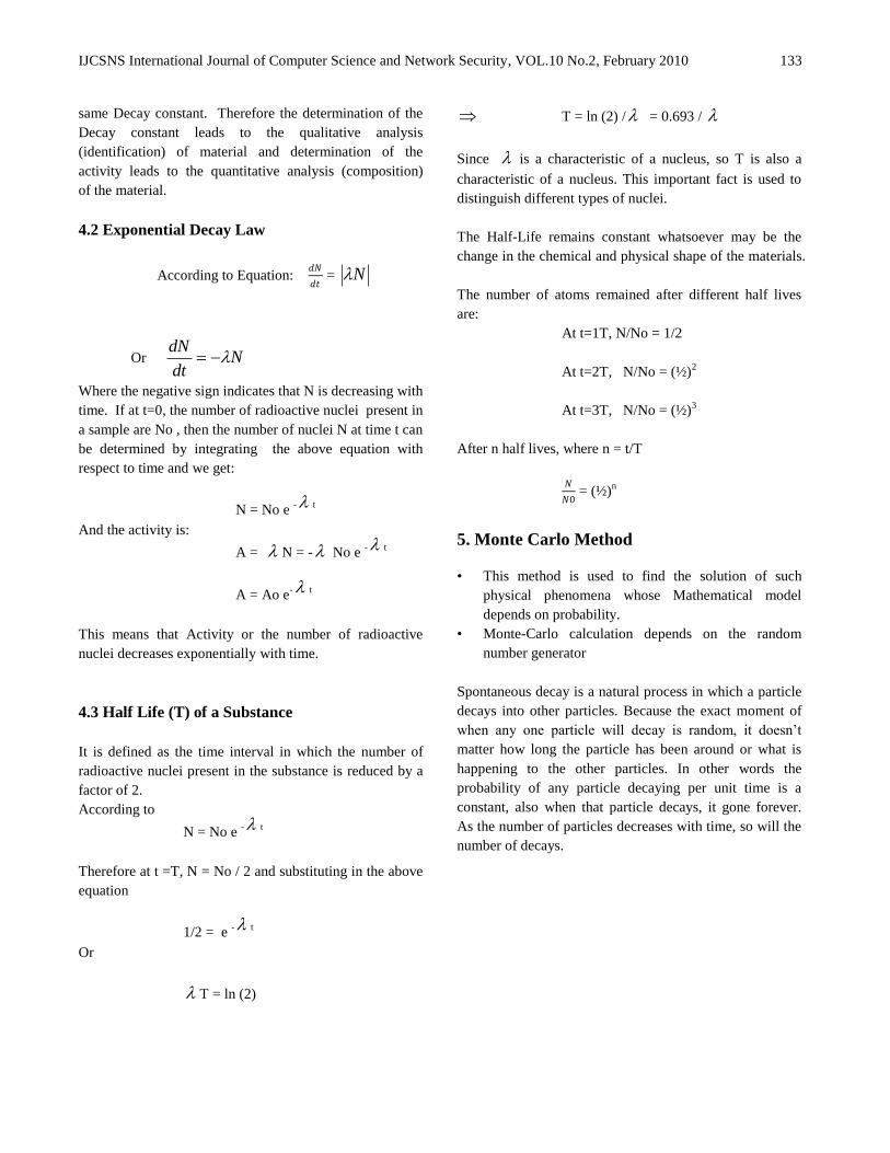
6.1 Radioactive Decay Simulation
Fig 6.1.1
6.1.1 Decay Simulation Algorithm
Start
1. input N, lambda;
2. initialize delN = 0,decay
3. loop (while N !=0)
decay = Random number b/w 0-1
If (decay < lambda)
delN = delN +1
N = N-delN.
End loop
4. Output Display graph of N , DelN
End
6.1.2 Procedure to use the Decay VI:
1. Select the total number of nuclides in the sample
using the KNOB “n0”.
2. Select the Decay parameter of the element used in
the sample using the KNOB “lambda”.
3. Press Ctrl+R to run the simulation.
4. Read data from indicators.
5. Read Data from the graph (Logarithmic curve of
n0) using the cursor legends, drag the yellow
cursors upon any two diff places on the curve.
6. Determine the slope of the curve, where slope =
decay parameter.
7. Put the value of slope in slope control and it will
calculate the half life of the element.
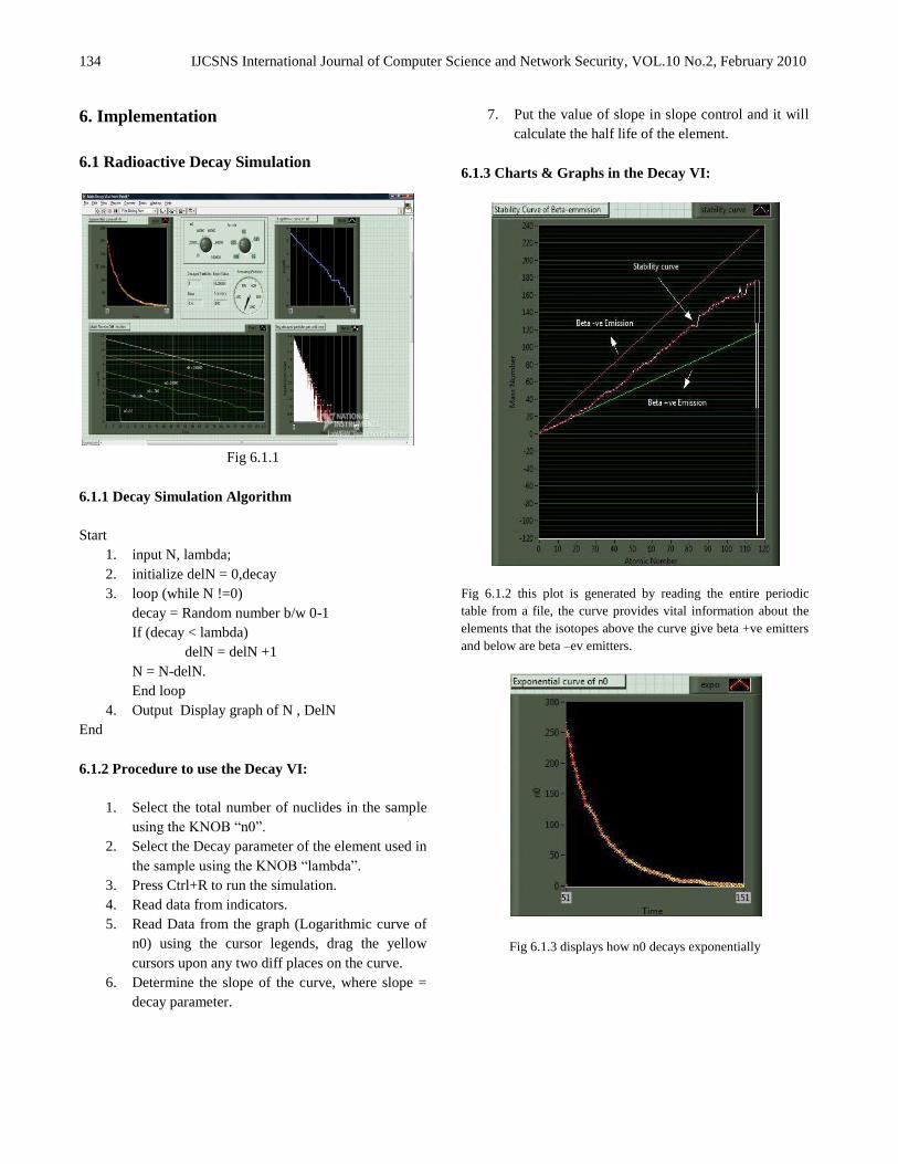
6.1.3 Charts & Graphs in the Decay VI:
Fig 6.1.2 this plot is generated by reading the entire periodic
table from a file, the curve provides vital information about the
elements that the isotopes above the curve give beta +ve emitters
and below are beta –ev emitters.
Fig 6.1.3 displays how n0 decays exponentially
IJCSNS International Journal of Computer Science and Network Security, VOL.10 No.2, February 2010
135
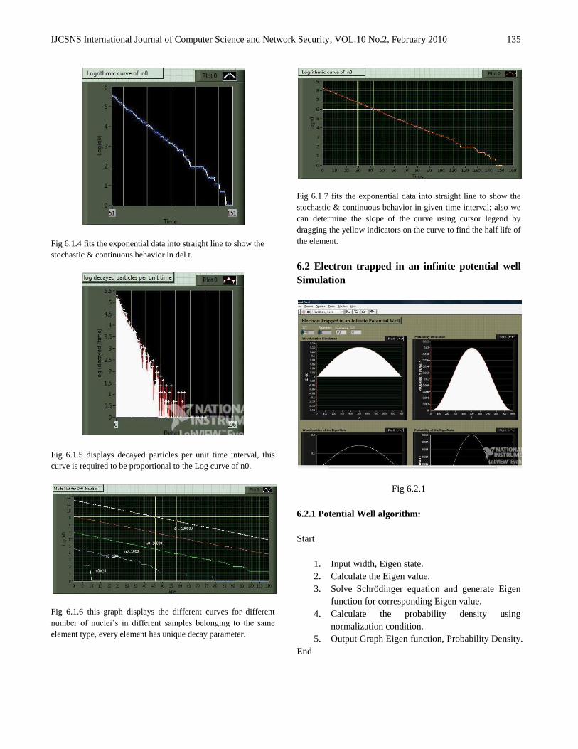
Fig 6.1.4 fits the exponential data into straight line to show the
stochastic & continuous behavior in del t.
Fig 6.1.5 displays decayed particles per unit time interval, this
curve is required to be proportional to the Log curve of n0.
Fig 6.1.6 this graph displays the different curves for different
number of nuclei‟s in different samples belonging to the same
element type, every element has unique decay parameter.
Fig 6.1.7 fits the exponential data into straight line to show the
stochastic & continuous behavior in given time interval; also we
can determine the slope of the curve using cursor legend by
dragging the yellow indicators on the curve to find the half life of
the element.
6.2 Electron trapped in an infinite potential well
Simulation
Fig 6.2.1
6.2.1 Potential Well algorithm:
Start
1. Input width, Eigen state.
2. Calculate the Eigen value.
3. Solve Schrödinger equation and generate Eigen
function for corresponding Eigen value.
4. Calculate the probability density using
normalization condition.
5. Output Graph Eigen function, Probability Density.
End
IJCSNS International Journal of Computer Science and Network Security, VOL.10 No.2, February 2010
136
6.2.2 Procedure to use the VI:
1. Input width of the potential well in the control “-L/2”.
2. Input Eigen state (quantum number) in the control
“Eigen states”.
3. Press Ctrl+R to run the simulation.
4. The “Eigen value” indicator gives output
corresponding to the quantum number.
5. Read data from plots by placing cursor on different
points to find energy at that point.
6. Also use multi-state plot to find variations in different
Eigen functions.
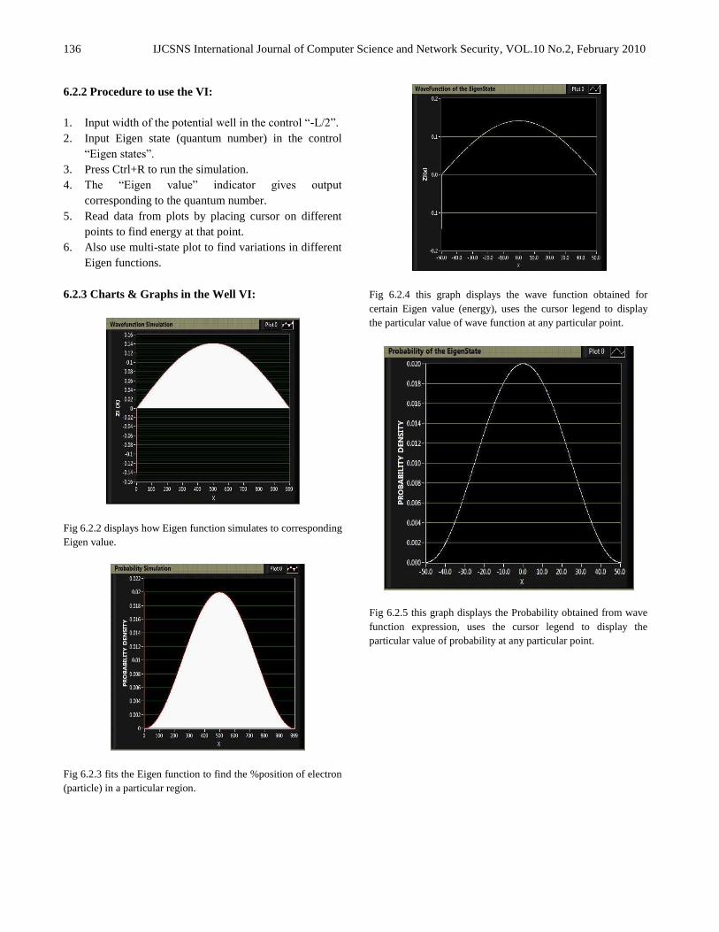
6.2.3 Charts & Graphs in the Well VI:
Fig 6.2.2 displays how Eigen function simulates to corresponding
Eigen value.
Fig 6.2.3 fits the Eigen function to find the %position of electron
(particle) in a particular region.
Fig 6.2.4 this graph displays the wave function obtained for
certain Eigen value (energy), uses the cursor legend to display
the particular value of wave function at any particular point.
Fig 6.2.5 this graph displays the Probability obtained from wave
function expression, uses the cursor legend to display the
particular value of probability at any particular point.
IJCSNS International Journal of Computer Science and Network Security, VOL.10 No.2, February 2010
137
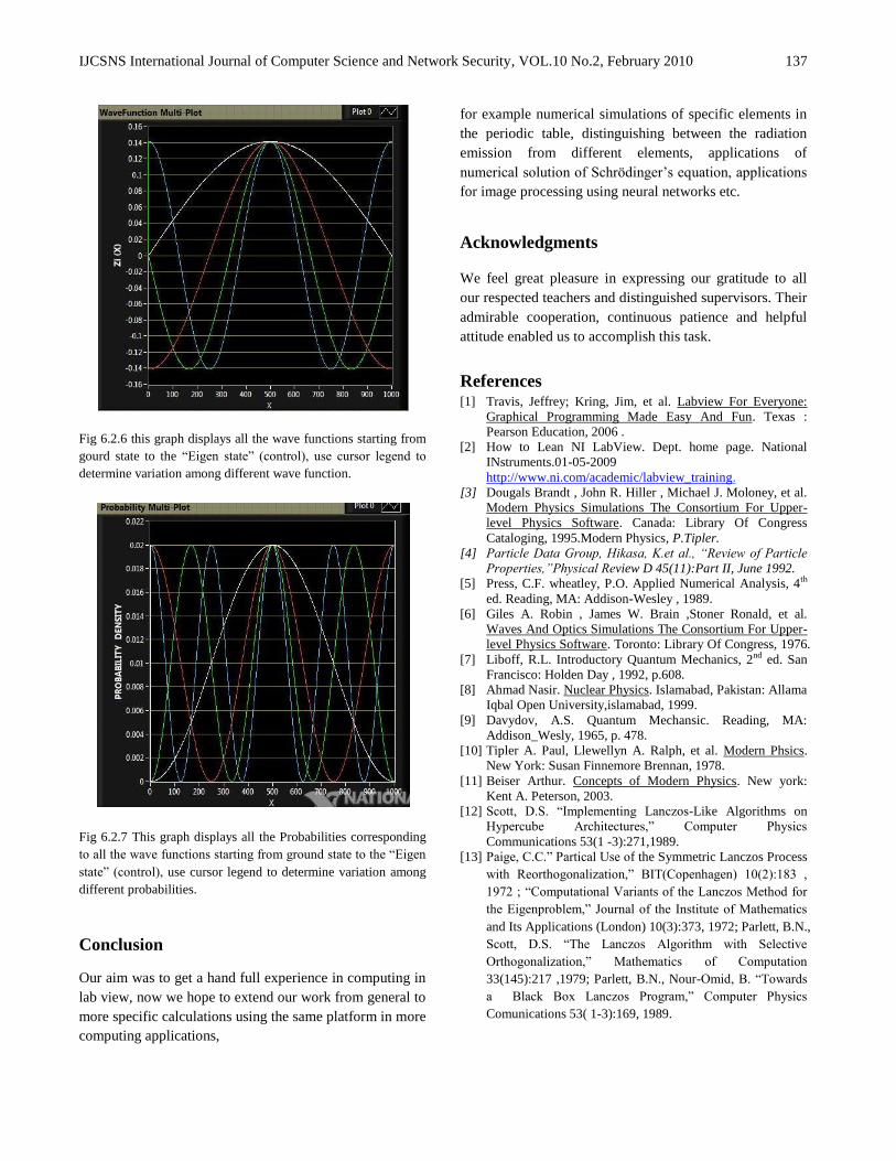
Fig 6.2.6 this graph displays all the wave functions starting from
gourd state to the “Eigen state” (control), use cursor legend to
determine variation among different wave function.
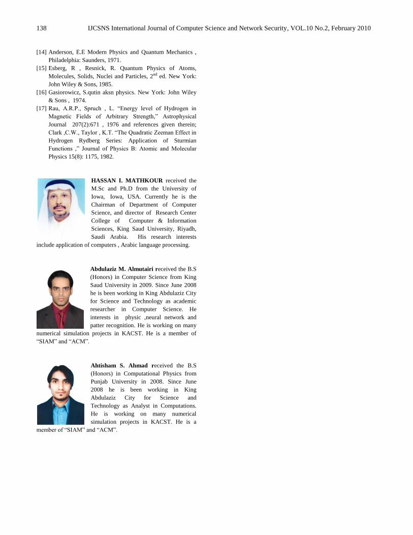
Fig 6.2.7 This graph displays all the Probabilities corresponding
to all the wave functions starting from ground state to the “Eigen
state” (control), use cursor legend to determine variation among
different probabilities.
Conclusion
Our aim was to get a hand full experience in computing in
lab view, now we hope to extend our work from general to
more specific calculations using the same platform in more
computing applications,
for example numerical simulations of specific elements in
the periodic table, distinguishing between the radiation
emission from different elements, applications of
numerical solution of Schrödinger‟s equation, applications
for image processing using neural networks etc.
Acknowledgments
We feel great pleasure in expressing our gratitude to all
our respected teachers and distinguished supervisors. Their
admirable cooperation, continuous patience and helpful
attitude enabled us to accomplish this task.
References [1] Travis, Jeffrey; Kring, Jim, et al. Labview For Everyone:
Graphical Programming Made Easy And Fun. Texas :
Pearson Education, 2006 .
[2] How to Lean NI LabView. Dept. home page. National
INstruments.01-05-2009
http://www.ni.com/academic/labview_training.
[3] Dougals Brandt , John R. Hiller , Michael J. Moloney, et al.
Modern Physics Simulations The Consortium For Upper-
level Physics Software. Canada: Library Of Congress
Cataloging, 1995.Modern Physics, P.Tipler.
[4] Particle Data Group, Hikasa, K.et al., “Review of Particle
Properties,”Physical Review D 45(11):Part II, June 1992.
[5] Press, C.F. wheatley, P.O. Applied Numerical Analysis, 4th
ed. Reading, MA: Addison-Wesley , 1989.
[6] Giles A. Robin , James W. Brain ,Stoner Ronald, et al.
Waves And Optics Simulations The Consortium For Upper-
level Physics Software. Toronto: Library Of Congress, 1976.
[7] Liboff, R.L. Introductory Quantum Mechanics, 2nd ed. San
Francisco: Holden Day , 1992, p.608.
[8] Ahmad Nasir. Nuclear Physics. Islamabad, Pakistan: Allama
Iqbal Open University,islamabad, 1999.
[9] Davydov, A.S. Quantum Mechansic. Reading, MA:
Addison_Wesly, 1965, p. 478.
[10] Tipler A. Paul, Llewellyn A. Ralph, et al. Modern Phsics.
New York: Susan Finnemore Brennan, 1978.
[11] Beiser Arthur. Concepts of Modern Physics. New york:
Kent A. Peterson, 2003.
[12] Scott, D.S. “Implementing Lanczos-Like Algorithms on
Hypercube Architectures,” Computer Physics
Communications 53(1 -3):271,1989.
[13] Paige, C.C.” Partical Use of the Symmetric Lanczos Process
with Reorthogonalization,” BIT(Copenhagen) 10(2):183 ,
1972 ; “Computational Variants of the Lanczos Method for
the Eigenproblem,” Journal of the Institute of Mathematics
and Its Applications (London) 10(3):373, 1972; Parlett, B.N.,
Scott, D.S. “The Lanczos Algorithm with Selective
Orthogonalization,” Mathematics of Computation
33(145):217 ,1979; Parlett, B.N., Nour-Omid, B. “Towards
a Black Box Lanczos Program,” Computer Physics
Comunications 53( 1-3):169, 1989.
IJCSNS International Journal of Computer Science and Network Security, VOL.10 No.2, February 2010
138
[14] Anderson, E.E Modern Physics and Quantum Mechanics ,
Philadelphia: Saunders, 1971.
[15] Esberg, R , Resnick, R. Quantum Physics of Atoms,
Molecules, Solids, Nuclei and Particles, 2nd ed. New York:
John Wiley & Sons, 1985.
[16] Gasiorowicz, S.qutin aksn physics. New York: John Wiley
& Sons , 1974.
[17] Rau, A.R.P., Spruch , L. “Energy level of Hydrogen in
Magnetic Fields of Arbitrary Strength,” Astrophysical
Journal 207(2):671 , 1976 and references given therein;
Clark ,C.W., Taylor , K.T. “The Quadratic Zeeman Effect in
Hydrogen Rydberg Series: Application of Sturmian
Functions ,” Journal of Physics B: Atomic and Molecular
Physics 15(8): 1175, 1982.
HASSAN I. MATHKOUR received the
M.Sc and Ph.D from the University of
Iowa, Iowa, USA. Currently he is the
Chairman of Department of Computer
Science, and director of Research Center
College of Computer & Information
Sciences, King Saud University, Riyadh,
Saudi Arabia. His research interests
include application of computers , Arabic language processing.
Abdulaziz M. Almutairi received the B.S
(Honors) in Computer Science from King
Saud University in 2009. Since June 2008
he is been working in King Abdulaziz City
for Science and Technology as academic
researcher in Computer Science. He
interests in physic ,neural network and
patter recognition. He is working on many
numerical simulation projects in KACST. He is a member of
“SIAM” and “ACM”.
Ahtisham S. Ahmad received the B.S
(Honors) in Computational Physics from
Punjab University in 2008. Since June
2008 he is been working in King
Abdulaziz City for Science and
Technology as Analyst in Computations.
He is working on many numerical
simulation projects in KACST. He is a
member of “SIAM” and “ACM”.