In Wiley Interdisciplinary Reviews: Cognitive Science (4) 4, 2013

1

Computational Models of Planning(Overview Article)

Hector GeffnerICREA & Universitat Pompeu Fabra

Roc Boronat 138, 55.21308018 Barcelona, SPAIN

Abstract

The selection of the action to do next is one of the central problems faced byautonomous agents. Natural and artificial systems address this problem in variousways: action responses can be hardwired, they can be learned, or they can be computedfrom a model of the situation, the actions, and the goals. Planning is the model-based approach to action selection and a fundamental ingredient of intelligent behaviorin both humans and machines. Planning, however, is computationally hard as theconsideration of all possible courses of action is not computationally feasible. Theproblem has been addressed by research in Artificial Intelligence that in recent years hasuncovered simple but powerful computational principles that make planning feasible.The principles take the form of domain-independent methods for computing heuristicsor appraisals that enable the effective generation of goal-directed behavior even overhuge spaces. In this paper, we look at several planning models, at methods that havebeen shown to scale up to large problems, and at what these methods may suggestabout the human mind.

1 Introduction

Planning is one of the key aspects of intelligent behavior, and one of the first to be studied inthe field of Artificial Intelligence (AI). The first AI planner and one of the first AI programswas the General Problem Solver (GPS) developed by Newell and Simon in the late 50’s[80, 81]. Since then, planning has remained a central topic in AI while changing in significantways: on the one hand, it has become more rigorous, with a variety of planning modelsdefined and studied; on the other, it has become more empirical, with planning algorithmsevaluated experimentally and a strong emphasis placed on scalability: effective goal-orientedbehavior that is not limited by the number of actions and variables in the problem.

Planning can be understood as representing one of the three main approaches for selectingthe action to do next ; a problem that is central in the design of autonomous systems. Inthe hardwired approach, action responses are hardwired by nature, or more commonly in AIsystems, by a programmer. For a robot moving in an office environment, for example, the

1

2

program may say to back up when too close to a wall, to search for a door if the robot has tomove to another room, and so on [25, 71]. The problem with this approach, common to manyother AI systems, is that since it is difficult to anticipate all possible situations and the bestway to handle them, the resulting systems tend to be brittle. In the learning-based approach,on the other hand, action responses are not hardwired but are learned by trial and error as inreinforcement learning [98], or by generalization from examples as in supervised learning [78,89]. Finally, in the model-based approach, action responses are computed from a model of thesituation, the actions, the sensors, and goals [89, 39, 37]. The distinction that the philosopherDaniel Dennett makes between ‘Darwinian’, ‘Skinnerian’, and ‘Popperian’ creatures [32],mirrors quite closely the distinction between hardwired agents, agents that learn, and agentsthat use models respectively. The approaches, however, are not incompatible, and indeed,agents that learn models rather than behavioral responses fit also in the latter class, as theymust then use the models learned for selecting the action to do next.

Planning, usually associated with “thinking before acting”, is best conceived as themodel-based approach to action selection. It is a fundamental ingredient of intelligent be-havior in both humans and machines, yet it is computationally hard. Indeed, even in themost simple planning model where the state of the world is fully known and actions havedeterministic effects, the number of possible world states is exponential in the number ofstate variables, and the number of possible plans is exponential in the length of the plans.1

The situation facing an artificial agent that plans even in the simplest setting, has a keyelement that is common with humans making plans: neither one can afford to considerall possible courses of action as this is not computationally feasible. This computationalchallenge has been used as evidence for contesting the possibility of general planning andreasoning abilities in humans or machines [100]. The complexity of planning, however, justimplies that no planner can efficiently solve every problem from every domain, not that aplanner cannot solve an infinite collection of problems from old and new domains, and hencebe useful to an acting agent. This is indeed the way modern AI planners are empiricallyevaluated and ranked in AI planning competitions, where they are tried on domains thatthe planners’ authors have never seen [29]. Thus, far from representing an insurmountableobstacle, the twin requirements of generality and scalability have been addressed head onin AI planning research, and this has led to simple but powerful computational principlesthat make domain-independent planning feasible. The principles take the form of heuristicsor appraisals that are computed automatically for the problem at hand from suitable relax-ations (simplifications) of the problem. The heuristics derived in this way tailor the generalsolver to the specific problem, and enable the generation of goal-directed behavior even overhuge spaces. In this paper, we look at these methods and what they may reveal about thehuman mind, turning the requirements of generality and scalability from an impossibilityinto a critical source of insight.

From a cognitive perspective, one lesson to draw is that if one of the primary roles offeelings and emotions is to act as rough guides in the generation of behavior in complexphysical and social worlds where the consideration of all possible courses of action is not

1More precisely, in the language of computer science, planning is said to be NP-hard, meaning thatthere cannot be a general sound and complete planning algorithm that runs in polynomial time, unlessthe fundamental conjecture in computer science that NP-hard problems do not admit polynomial solutions,widely believed to be true, turns out to be false [26].

2

2

computationally feasible, much is much to be gained by looking at suitable abstractions ofthe problem that present the same computational challenges in crisp form. More specifically,we will argue that the domain-independent methods for deriving heuristic functions thathave been developed for making planning feasible provide a different angle from which tolook at the computation and role of emotional appraisals in humans [36].2

The paper is organized as follows. We consider the most basic planning model first,the computational challenges that it presents, and the domain-independent methods thathave been developed for addressing this challenge. We then look at what these domain-independent heuristics suggest about the generation, nature, and role of unconscious ap-praisals, and move on to alternative planning methods and richer planning models. We con-clude by discussing some open challenges in planning research and summarizing the mainlessons.

2 Basic Model: Classical Planning

The most basic model in planning is concerned with the selection of actions for achievinggoals when the initial situation is fully known and actions have deterministic effects. Themodel underlying this form of planning, called classical planning, can be described formallyin terms of a state space featuring

• a finite and discrete set of states S,

• a known initial state s0 ∈ S,

• a set SG ⊆ S of goal states,

• a set of actions A(s) ⊆ A applicable in each state s ∈ S,

• a deterministic state transition function f(a, s) for a ∈ A(s) and s ∈ S, so that f(a, s)denotes the state that results from doing action a in state s, and

• positive action costs c(a, s) that may depend on the action a and the state s.

A solution or plan for this model is a sequence of actions a0, . . . , an that generates a statesequence s0, s1, . . . , sn+1 such that each action ai is applicable in the state si and results inthe state si+1 = f(ai, si), the last of which is a goal state; i.e., si+1 = f(ai, si) for ai ∈ A(si),i = 0, . . . , n, and sn+1 ∈ SG. The cost of a plan is the sum of the action costs c(ai, si), anda plan is optimal if it has minimum cost. The cost of a problem is the cost of its optimalsolutions. When action costs are all one, plan cost reduces to plan length, and the optimalplans are simply the shortest ones.

As an illustration, the problem of rearranging a set of block towers into a different setof towers can be naturally formulated as a model of this type where the state representsthe possible block configurations. Similarly, delivering a set of goods to clients, solving a

2The relationship between planning and emotion has been considered by other authors that aim toimport elements from the theory of emotions into AI planners [43, 44]. Our focus here goes in the oppositedirection, on what modern computational models of planning can tell us about the generation, nature, androle of emotional appraisals.

3

2

puzzle such as Rubik’s Cube, or playing solitaire can be all expressed as classical planningproblems.

The model underlying classical planning does not account for either uncertainty or sens-ing, and thus gives rise to plans that represent open-loop controllers where observations playno role. Planning models that take these aspects into account give rise to different types ofcontrollers and will be considered later.

3 State Variables and Factored Representations

The state models required for planning are not represented explicitly in general because theyare often too large. The planning agent is assumed to have instead a compact and implicitrepresentation of the state model given in terms of a set of state variables. The states arethe possible combination of values over these variables, and the actions are defined in termsof pre and postconditions expressed over the state variables as well.

One of the most common languages for representing classical planning problems is alsoone of the oldest, Strips [35], a planning language that can be traced back to the late 60’s.A planning problem in Strips is a tuple P = 〈F,O, I,G〉 where

• F represents a set of boolean variables,

• O represents a set of actions,

• I represents the initial situation, and

• G represents the goal.

Both the initial situation I and the goal G are expressed by a set of atoms over F . Fora boolean state variable p in F , there are two atoms p = true and p = false, abbreviatedusing logical notation as p and ¬p, where the symbol ‘¬’ stands for negation. A state in aStrips problem is a valuation of the state variables represented by the collection of atomsthat the state makes true. The initial situation I stands for the state that makes the atomsin I true and all other atoms false, while the goal G stands for the collection of states thatmake all the atoms in G true.

In Strips, the actions o ∈ O are represented by three sets of atoms over F called theAdd, Delete, and Precondition lists, denoted as Add(o), Del(o), Pre(o). The first describesthe atoms that the action o makes true, the second, the atoms that o makes false, and thethird, the atoms that must be true in order for the action to be applicable. A Strips problemP = 〈F,O, I,G〉 encodes implicitly, in compact form, the classical state model S(P ) where

• the states s ∈ S are the possible collections of atoms over F ,

• the initial state s0 is I,

• the goal states s are those for which G ⊆ s,

• the actions a in A(s) are the ones in O with Prec(a) ⊆ s,

• the state transition function is f(a, s) = (s \ Del(a)) ∪ Add(a), i.e., the state s withthe atoms in Del(a) deleted and the atoms in Add(a) added, and

• the action costs c(a) are equal to one by default.

4

2

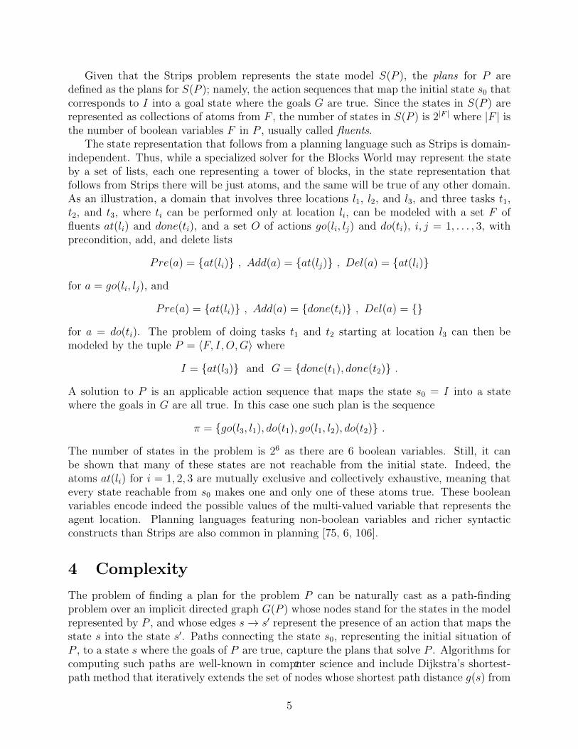
Given that the Strips problem represents the state model S(P ), the plans for P aredefined as the plans for S(P ); namely, the action sequences that map the initial state s0 thatcorresponds to I into a goal state where the goals G are true. Since the states in S(P ) arerepresented as collections of atoms from F , the number of states in S(P ) is 2|F | where |F | isthe number of boolean variables F in P , usually called fluents.

The state representation that follows from a planning language such as Strips is domain-independent. Thus, while a specialized solver for the Blocks World may represent the stateby a set of lists, each one representing a tower of blocks, in the state representation thatfollows from Strips there will be just atoms, and the same will be true of any other domain.As an illustration, a domain that involves three locations l1, l2, and l3, and three tasks t1,t2, and t3, where ti can be performed only at location li, can be modeled with a set F offluents at(li) and done(ti), and a set O of actions go(li, lj) and do(ti), i, j = 1, . . . , 3, withprecondition, add, and delete lists

Pre(a) = {at(li)} , Add(a) = {at(lj)} , Del(a) = {at(li)}

for a = go(li, lj), and

Pre(a) = {at(li)} , Add(a) = {done(ti)} , Del(a) = {}

for a = do(ti). The problem of doing tasks t1 and t2 starting at location l3 can then bemodeled by the tuple P = 〈F, I, O,G〉 where

I = {at(l3)} and G = {done(t1), done(t2)} .

A solution to P is an applicable action sequence that maps the state s0 = I into a statewhere the goals in G are all true. In this case one such plan is the sequence

π = {go(l3, l1), do(t1), go(l1, l2), do(t2)} .

The number of states in the problem is 26 as there are 6 boolean variables. Still, it canbe shown that many of these states are not reachable from the initial state. Indeed, theatoms at(li) for i = 1, 2, 3 are mutually exclusive and collectively exhaustive, meaning thatevery state reachable from s0 makes one and only one of these atoms true. These booleanvariables encode indeed the possible values of the multi-valued variable that represents theagent location. Planning languages featuring non-boolean variables and richer syntacticconstructs than Strips are also common in planning [75, 6, 106].

4 Complexity

The problem of finding a plan for the problem P can be naturally cast as a path-findingproblem over an implicit directed graph G(P ) whose nodes stand for the states in the modelrepresented by P , and whose edges s→ s′ represent the presence of an action that maps thestate s into the state s′. Paths connecting the state s0, representing the initial situation ofP , to a state s where the goals of P are true, capture the plans that solve P . Algorithms forcomputing such paths are well-known in computer science and include Dijkstra’s shortest-path method that iteratively extends the set of nodes whose shortest path distance g(s) from

5

2

B C

A

C

A

B A B CB

A

C

B

C

A

A

B

C

C

A B A

B

C

C

BA

A B CA

B

C

B

C

A

......... ........

GOAL

GOALINIT

.....

.....

....

....

Figure 1: The graph corresponding to a simple planning problem involving three blocks with initialand goal situations I and G as shown. The actions allow moving a clear block on top of anotherclear block or to the table. The size of the complete graph for this domain is exponential in thenumber of blocks. A plan for the problem is shown by the path in red.

the source node is labeled as known, starting with the set that comprises only the sourcenode s0 [33, 30]. Then, in each iteration, Dijkstra’s algorithm selects among the nodes swhose shortest path distance from s0 is not yet known, the one that minimizes the distanceg(s) = mins′ g(s′)+c(s′, s), where s′ ranges over the nodes that can be mapped into the states by an action with cost c(s′, s). The algorithm then labels the distance g(s) to the state s asknown, and iterates until no more states can be labeled in this manner. The algorithm canbe stopped when the node selected is a goal node. The measure g(s) for that node encodesthe cost of a cheapest plan that solves the planning problem P .

Algorithms for solving path-finding problems over directed graphs such as Dijkstra’salgorithm run in time that is polynomial in the number of nodes in the graph. This, however,is not good enough in planning where the number of nodes is exponential in the number ofproblem variables F . Since in Strips the variables are boolean, the number of nodes in thegraph to search can be in the order of 2|F |. For example, if the problem involves 30 variables,the number of nodes in the graph is 1, 073, 741, 824, and if it involves 100 variables, thenumber of nodes is larger than 1030. If it takes 1 second to generate 107 nodes (a realisticestimate given current technology), it would take more than 1023 seconds to generate allnodes in the latter case. This is however almost one million times the estimated age of theuniverse.3 Planning algorithms able to deal with tens of variables or more thus cannot bebased on exhaustive methods such as Dijkstra’s, and need to search for paths in graphs in amore focused manner.

A more concrete illustration of the complexity inherent in the planning problem can

3The age of the universe is estimated at 13.7 × 109 years approximately. Generating 2100 nodes at 107

nodes a second would take in the order of 1015 years, as 2100/(107 ∗ 60 ∗ 60 ∗ 24 ∗ 365) ≈ 4 ∗ 1015.

6

2

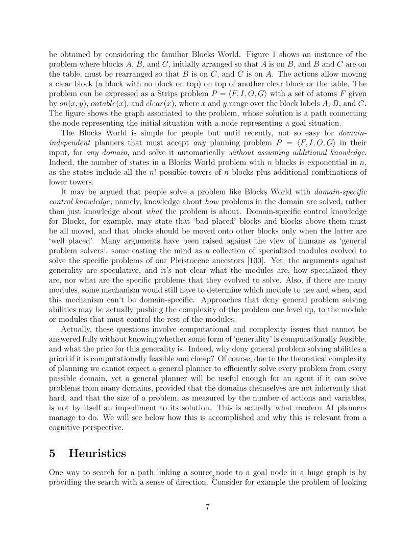
be obtained by considering the familiar Blocks World. Figure 1 shows an instance of theproblem where blocks A, B, and C, initially arranged so that A is on B, and B and C are onthe table, must be rearranged so that B is on C, and C is on A. The actions allow movinga clear block (a block with no block on top) on top of another clear block or the table. Theproblem can be expressed as a Strips problem P = 〈F, I, O,G〉 with a set of atoms F givenby on(x, y), ontable(x), and clear(x), where x and y range over the block labels A, B, and C.The figure shows the graph associated to the problem, whose solution is a path connectingthe node representing the initial situation with a node representing a goal situation.

The Blocks World is simple for people but until recently, not so easy for domain-independent planners that must accept any planning problem P = 〈F, I, O,G〉 in theirinput, for any domain, and solve it automatically without assuming additional knowledge.Indeed, the number of states in a Blocks World problem with n blocks is exponential in n,as the states include all the n! possible towers of n blocks plus additional combinations oflower towers.

It may be argued that people solve a problem like Blocks World with domain-specificcontrol knowledge; namely, knowledge about how problems in the domain are solved, ratherthan just knowledge about what the problem is about. Domain-specific control knowledgefor Blocks, for example, may state that ‘bad placed’ blocks and blocks above them mustbe all moved, and that blocks should be moved onto other blocks only when the latter are‘well placed’. Many arguments have been raised against the view of humans as ‘generalproblem solvers’, some casting the mind as a collection of specialized modules evolved tosolve the specific problems of our Pleistocene ancestors [100]. Yet, the arguments againstgenerality are speculative, and it’s not clear what the modules are, how specialized theyare, nor what are the specific problems that they evolved to solve. Also, if there are manymodules, some mechanism would still have to determine which module to use and when, andthis mechanism can’t be domain-specific. Approaches that deny general problem solvingabilities may be actually pushing the complexity of the problem one level up, to the moduleor modules that must control the rest of the modules.

Actually, these questions involve computational and complexity issues that cannot beanswered fully without knowing whether some form of ‘generality’ is computationally feasible,and what the price for this generality is. Indeed, why deny general problem solving abilities apriori if it is computationally feasible and cheap? Of course, due to the theoretical complexityof planning we cannot expect a general planner to efficiently solve every problem from everypossible domain, yet a general planner will be useful enough for an agent if it can solveproblems from many domains, provided that the domains themselves are not inherently thathard, and that the size of a problem, as measured by the number of actions and variables,is not by itself an impediment to its solution. This is actually what modern AI plannersmanage to do. We will see below how this is accomplished and why this is relevant from acognitive perspective.

5 Heuristics

One way to search for a path linking a source node to a goal node in a huge graph is byproviding the search with a sense of direction. Consider for example the problem of looking

7

2

on a map for a good route between Los Angeles (LA) and New York (NY), regarding themap as a graph whose nodes are cities, and whose edges connect pairs of cities throughdirected routes at a cost proportional to the route length. Dijkstra’s algorithm, sketchedabove, provides a way for finding routes in such graphs. If our map covers all of NorthAmerica, however, the algorithm would appear to behave in a strange manner, finding firstshortest paths to all cities that are closer to LA than NY (like Mexico City) whether theyare on the way to NY or not. The search in such a case is said to be blind, meaning thatinformation about the goal is not used in the exploration of the map. This is definitelynot the way that people search for routes in a map. If they want to go to a city that isNortheast, they will look for routes headed in that direction. The search is then focused andthe total number of cities in the map is less of a problem. This basic intuition about goal-directed search was incorporated into AI search algorithms in the 60’s and 70’s in the formof heuristic functions : functions h(s) that provide a quick-and-dirty estimate of the distanceor cost separating a state s from a goal state. In the route finding problem, for example,a useful heuristic h(s) is the Euclidean distance separating a city s from the target city.This is a heuristic that is very easy to compute and which provides a good approximationof the optimal cost h∗(s) of reaching the goal from s, whose exact computation would bemuch harder (as hard indeed as solving the original problem). Interestingly, if the evaluationfunction g(s) used to select the next node to label in Dijkstra’s algorithm is replaced by themore informed function f(s) = g(s) + h(s) that incorporates both the cost from s0 to s andan estimate of the cost to go from s to the goal, an heuristic search algorithm known as A*is obtained that can look for paths to the goal much more effectively [45].4 Heuristic searchalgorithms express a form of goal-driven search, where the goal is no longer passive in thesearch process, but actively biases the search through the heuristic term h(s). In the extremecase in which the heuristic h(s) is perfect, i.e., the estimates h(s) and the true costs h∗(s)coincide for all states, A* goes straight to the goal with no search at all. At the same time,if the heuristic is completely uninformative, as the null heuristic h(s) = 0 for all states, A*reduces to Dijkstra’s algorithm. In the middle, when 0 ≤ h(s) ≤ h∗(s) for all s, the heuristich is said to be admissible and A* preserves the optimality properties of Dijkstra but doesless work. Indeed, the closer to h∗, the more informed the heuristic, and the less number ofstates that are visited in the search. Heuristic search methods have been used for findingoptimal solutions to problems like Rubik’s Cube that involve more than 1019 states. Thekey is the use of suitable admissible heuristic functions h(s) that allow for optimal solutionswhile considering a tiny fraction of the problem states [65].

6 Domain-independent Generation of Heuristics

Heuristic search algorithms express a form of goal-directed search where heuristic functionsare used to guide the search towards the goal. A key question is how such heuristics canbe obtained for a given problem. A useful heuristic is one that provides good estimatesof the cost to the goal and can be computed reasonably fast. Heuristics are traditionallydevised according to the problem at hand: the Euclidean distance is a good heuristic for

4This description of A* assumes that the heuristic is monotonic. A more complete description of A* andvariations can be found in the standard textbooks [84, 89].

8

2

Figure 2: The sliding 15-puzzle where the goal is to get to a configuration where the tiles areordered by number with the empty square last. The actions allowed are those that slide a tileinto the empty square. While the problem is not simple, the heuristic that sums the horizontaland vertical distances of each tile to its target position is simple to compute and provides aninformative estimate of the number of steps to the goal. In planning, heuristic functions areobtained automatically from the problem representation.

route finding, the sum of the Manhattan distances of each tile to its destination is a goodheuristic for the sliding puzzles, and so on.5 The general idea that emerges from the variousheuristics developed for different problems is that heuristics h(s) can be seen as encoding thecost of reaching the goal from the state s in a problem that is simpler than the original one[95, 77, 84]. For example, the sum of the Manhattan distances in the sliding puzzles (Fig. 2),corresponds to the optimal cost of a simplification of the puzzle where tiles can be movedto adjacent positions, whether such positions are empty or not. Similarly, the Euclideanheuristic for route finding is the cost of a simplification where straight routes are addedbetween any pair of cities. The simplified problems are normally referred to as relaxationsof the original problem.

The key development in modern planning research in AI was the realization that usefulheuristics could be derived automatically from the representation of the problem in a domain-independent language such as Strips [74, 18, 13]. It does not matter what the problem isabout, a domain-independent relaxation is obtained directly and effectively from the problemrepresentation from which heuristics that are adapted to the problem can be computed.

The most common and useful domain-independent relaxation in planning is the delete-relaxation that maps a problem P = 〈F, I, O,G〉 in Strips into a problem P+ = 〈F, I, O+, G〉that is exactly like P but with the actions in O+ set to the actions in O with empty deletelists. That is, the delete-relaxation is a domain-independent relaxation that takes a planningproblem P and produces another problem P+ where atoms are added exactly like in P butwhere atoms are never deleted. The relaxation implies, for example, that objects and agentscan be in “multiple places” at the same time, as when an object or an agent moves into anew place, the atom encoding the old location is not deleted. Relaxations, however, are notaimed at providing accurate models of the world; quite the opposite, simplified and even

5The Manhattan distance of a tile is the sum of the horizon and vertical distances that separate its currentposition from its destination.

9

2

meaningless models of the world that while not accurate yield useful heuristics.The domain-independent delete-relaxation heuristic is obtained as an approximation of

the optimal cost of the delete-relaxation P+, obtained from the cost of a plan that solves P+

not necessarily optimally.6 The reason that an approximation is needed is because finding anoptimal plan for a delete-free planning problem like P+ is still a computationally intractabletask (also NP-hard). On the other hand, finding just one plan for the relaxation whetheroptimal or not, can be done quickly and efficiently. The property that allows for this isdecomposability: a problem without deletes is decomposable in the sense that a plan π for ajoint goal G1 and G2 can always be obtained from a plan π1 for the goal G1 and a plan π2for the goal G2. Indeed, it can be shown that the concatenation of the two plans π = π1, π2in either order, is one such plan. This property allows for a simple method for computingplans for the relaxation from which the heuristics are derived.

The main idea behind the procedure for computing the heuristic h(s) for an arbitraryplanning problem P can be explained in a few lines. For this, let P (s) refer to the problemthat is like P but with the initial situation set to the state s, and let P+(s) stand for thedelete-relaxation of P (s), i.e., the problem that is like P (s) but where the delete-lists areempty. The heuristic h(s) is computed from a plan for the relaxation P+(s) that is obtainedusing the decomposition property and a simple iteration. Basically, the plans for achievingthe atoms p that are already true in the state s, i.e., p ∈ s, are the empty plans, and ifπ1, π2, . . . , πm are the plans for achieving each of the preconditions p1, p2, . . . , pm of anaction a that has the atom q in the add list, π = π1, π2, . . . , πm followed by the action a isa plan for achieving q. It can be shown that this iteration yields a plan in the relaxationP+(s) for each atom p that has a plan in the original problem P (s), in a number of stepsthat is bounded by the number of variables in the problem. A plan for the actual goal Gof P (s) in the relaxation P+(s) can be obtained in a similar manner by just concatenatingthe plans for each of the atoms q in G in any order. Such a plan for the relaxation P+(s),denoted as π+(s), is usually called the relaxed plan. The heuristic h(s) is set to the cost ofsuch a plan. A better estimate can be obtained if duplicate actions are removed every timeplans are concatenated [58]. Other heuristics based also on the delete-relaxation such as theadditive heuristic [13] and the FF heuristic [48], are as informative as this heuristic but canbe computed faster. Notice that a plan π+(s) for the relaxation yields the heuristic valueh(s) that estimates the cost from s to the goal for the state s only. This computation thusmust be repeated for every state whose heuristic value is needed.

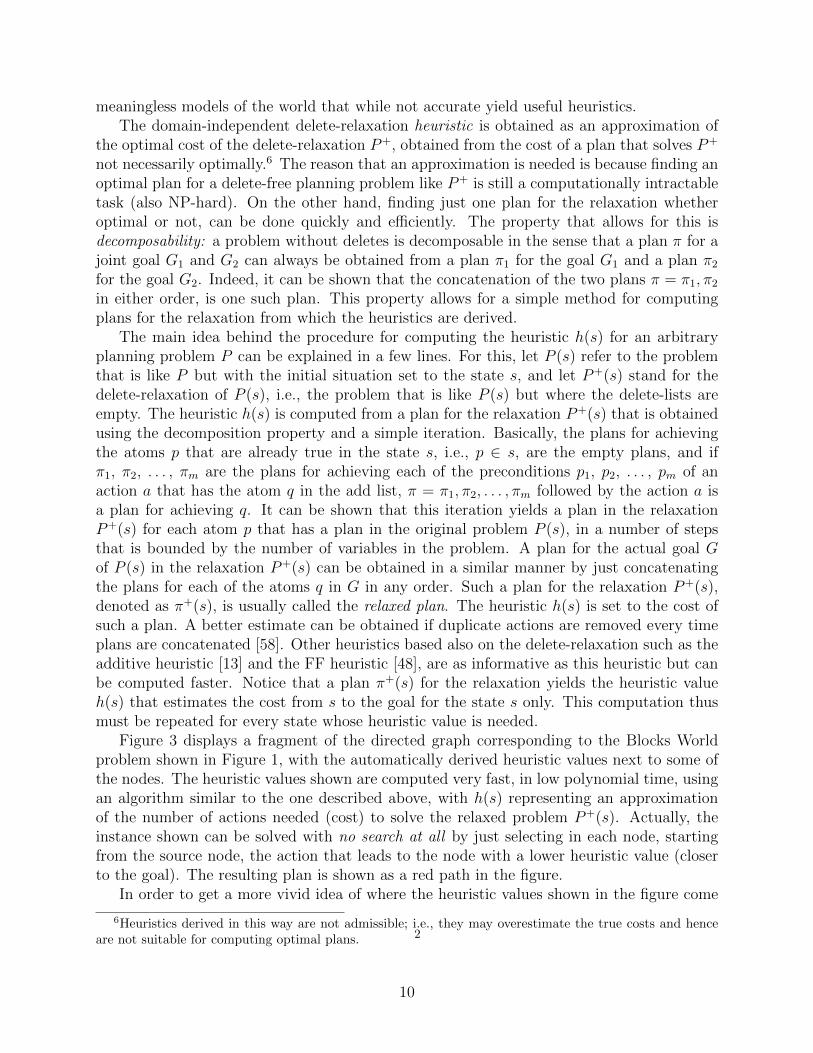
Figure 3 displays a fragment of the directed graph corresponding to the Blocks Worldproblem shown in Figure 1, with the automatically derived heuristic values next to some ofthe nodes. The heuristic values shown are computed very fast, in low polynomial time, usingan algorithm similar to the one described above, with h(s) representing an approximationof the number of actions needed (cost) to solve the relaxed problem P+(s). Actually, theinstance shown can be solved with no search at all by just selecting in each node, startingfrom the source node, the action that leads to the node with a lower heuristic value (closerto the goal). The resulting plan is shown as a red path in the figure.

In order to get a more vivid idea of where the heuristic values shown in the figure come

6Heuristics derived in this way are not admissible; i.e., they may overestimate the true costs and henceare not suitable for computing optimal plans.

10

2

B C

A

C

A

B A B CB

A

C

B

C

A

A

B

C

C

A B A

B

C

C

BA

A B CA

B

C

B

C

A

......... ........

GOAL

h=3

h=3h=2 h=3

h=1

h=0

h=2 h=2 h=2

h=2

GOALINIT

Figure 3: A fragment of the graph corresponding to the blocks problem with the automaticallyderived heuristic values next to some of the nodes. The heuristic values are computed in lowpolynomial time and provide the search with a sense of direction. The instance can actually besolved without any search by just performing in each state the action that leads to the node witha lower heuristic value (closer to the goal). The resulting plan is shown in red; helpful actions areshown in blue.

from, consider the heuristic h(s) for the initial state where block A is on B, and both B andC are on the table. In order to get the goal ‘B on C’ in the relaxation from the state s, twoactions are needed: one to get A out of the way to achieve the preconditions for moving B,the second to move B on top of C. On the other hand, in order to achieve the second goal‘C on A’ in the relaxation from s, just the action of moving C to A is needed. The resultis a heuristic value h(s) = 3 as shown, which actually coincides in this case with the cost ofthe best plan to achieve the joint goal from s in the non-relaxed problem P (s). Nonetheless,this is just a coincidence, and indeed, the best plans in the relaxation P+(s) can be quitedifferent than the best plans in the original problem P (s). The best plan for P (s) is unique,moving A to the table, then C on A, and finally B on C. On the other hand, a possibleoptimal plan in the relaxation P+(s) is to move first C on A, then A on the table, and finallyB on C. Of course, this plan does not make any sense in the real problem where A can’t bemoved when covered by C, yet the relaxation is not aimed at capturing the real problem orthe real physics, it is aimed at producing informative but quick estimates of the cost to thegoal. The reader can verify that for the leftmost child s′ of the initial state s, the costs ofthe problem P (s′) and the relaxation P+(s′) no longer coincide. The former is 4, while thelatter is 3, the difference arising from the goal ‘C on A’ that in the original problem mustbe undone and then redone. On the other hand, in the relaxation, this is never needed asno atom is ever deleted.

One last point about the domain-independent relaxation and the resulting heuristics: theautomatic computation of the heuristic value h(s) from a plan π+(s) for the relaxation P+(s)yields also relevant structural information that is not captured in the estimates themselves.

11

2

In particular, among all the actions that are applicable in the state s, the ‘relaxed plan’suggests the ones that appear as most relevant. These are the actions that are applicablein the state s and form part of the relaxed plan. In planning, such actions are said to be‘helpful’ [48], and this structural information is used too, in one way or another in everystate-of-the-art planner. Figure 3 shows the helpful actions in each of the states on theway to the goal by means of arrows depicted in blue. As it can be seen, two of the threeapplicable actions in the root state are helpful, just two of the six applicable actions arehelpful in the second state, and just one action is helpful in the last state before the goal. Itis not always the case that the best action in a state is among the ones found to be helpfulin that state, or among the ones leading to the children with lowest heuristic values, yet thisis often the case and this suffices for making the heuristic and the relaxation so useful. It isalso interesting that the notion of helpful actions that emerges from the relaxation suggestsa model for identifying the actions that appear as most promising in a state which doesnot require evaluating them first. This information can be used indeed for deciding whichactions to consider in a state, possibly ignoring the other actions. The resulting search isnot necessarily complete but it can be quite effective [48]. We will come back to this pointbelow.

7 Heuristic Search

Once a heuristic h(s) is available for estimating the cost to the goal from s, the question ishow to use it for finding a path to the goal. The simplest method for using the heuristic isby selecting the action a in s that produces the state s′ that appears to be closest to thegoal; i.e. the one with minimum h(s′) value. This algorithm is known as hill-climbing, fromits use in maximization problems, as it moves the search along the slope of the heuristicfunction h where a value h(s) = 0 denotes a goal. The problem with this and other localsearch algorithms is that they can get stuck in states where none of the children improveson (decreases) the heuristic value of the parent.

There are many heuristic search algorithms that avoid the problems of hill-climbing, andthey can be classified into two groups: off-line and on-line algorithms. If planning is thoughtof as “thinking before acting”, off-line search algorithms can be understood as thinking allthe way to the solution before acting, while on-line algorithms interleave thinking and acting.The algorithm A* described above is an off-line search algorithm with several guarantees:it is complete; i.e., it will find a solution if there is one, and it is optimal if the heuristich(s) is admissible (doesn’t overestimate true costs). On the other hand, an algorithm likehill-climbing can be used as an on-line algorithm that iteratively applies the action that leadsto the best child according to the heuristic. In the on-line setting, the algorithm is known asthe greedy algorithm; the name greedy implying that actions are selected fast after a shallowand quick lookahead. Of course, more informed versions of this greedy on-line algorithmcan be obtained by performing a deeper lookahead, with a lookahead of two levels, resultingin the action that leads to the best grandchild, a lookahead of three levels, resulting in theaction that leads to the best great grandchild, and so on. A similar idea is used in chessplaying programs that involve a slightly different model with adversarial agents [79, 89]. Twoproblems with greedy algorithms enhanced with a fixed depth lookahead are that they can

12

2

be trapped into a loop, returning to states that have been visited earlier in the execution,and that the computational effort grows exponentially with the lookahead depth. The loopproblem in the greedy algorithm has a very elegant and powerful solution: the algorithmLearning Real Time A* or LRTA* [64] behaves exactly as the greedy algorithm but onceit selects the action a in the state s, and before moving to the resulting state s′, it changesthe heuristic value h(s) to c(a, s) + h(s′), where c(a, s) is the cost of the action a in s, andh(s′) is the heuristic value of s′. If the problem has no states from which the goal cannotbe reached (dead-ends), this simple type of learning guarantees that the goal will eventuallybe reached, and moreover, that if the process is restarted many times while preserving theheuristic values that have been learned, the goal will eventually be reached optimally, ifthe initial heuristic is admissible. The algorithm LRTA* is also interesting because it canbe easily generalized to other models where actions have probabilistic effects and states arefully or partially observable. The generalized algorithm is known as Real-Time DynamicProgramming or RTDP [8, 14, 15]. One last on-line algorithm for probabilistic models thathas become popular in recent years due to its breakthrough performance in the game of Gois UCT [61, 38]. Closely related to UCT are on-line variants of AO* [17], an extension ofthe A* algorithm for models where actions have non-deterministic effects [68, 84].

8 Heuristics, Values, and Appraisals

Heuristic evaluation functions are used in other settings like chess playing programs andreinforcement learning. In chess, the evaluation functions are programmed by hand [79, 84],while in reinforcement learning, they are learned by trial-and-error [98]. Reinforcementlearning is a family of model-free methods that have been shown to be effective in low-leveltasks, and to provide an accurate account of learning in the brain [92]. Heuristic evaluationfunctions in domain-independent planning are computed instead using model-based methodswhere suitable relaxations are solved from scratch. These methods have been shown to workover large problems involving hundred of actions and fluents, and interesting lessons canbe drawn from these methods as well. Indeed, while feelings and emotions are currentlythought of as providing the appraisals that are necessary for navigating in a complex world[31], there are actually very few accounts of how such appraisals may be computed. Inplanning, the appraisals that manage to integrate information about the current situation,the goal, and the actions, for directing the agent towards the goal, are the heuristics computedfrom relaxations of the problem. The computational model of appraisals that is based onthe solution of relaxations that can be solved in low-polynomial time, suggests potentialexplanations for a number of observations. For example, the heuristics that result are ‘fastand frugal’ but unlike the heuristics considered by Gigerenzer and others [41, 40], they arealso general: they apply to all the problems that fit the classical planning model or thatcan be cast in that form. The use of relaxations can also potentially explain why appraisalsmay be opaque from a cognitive point of view, and thus not be conscious [104, 47, 54]. Thisis because the appraisals are obtained from a simplified model where, for example, objectscan be in different places at the same time, and hence where the meaning of the symbols isdifferent than the meaning of the symbols in the ‘true’ model. Finally, heuristic appraisalsprovide the agent with a sense of direction or ‘gut feeling’ that guide the action selection in

13

2

the presence of many alternatives, while avoiding an infinite regress in the decision process.Indeed, the computational role of these appraisals is to avoid or at least to reduce the need tosearch. Explicit evaluation of all possible courses of actions is not feasible computationally,and the heuristics provide the necessary focus. Actually, as discussed above, relaxation-basedheuristics in planning do not only provide an account of the value of the different options,but also of the actions that are worth evaluating; the so-called helpful actions [48]. Thissecond aspect, although not necessarily in this form, may potentially help to explain a keydifference between programs and humans in games such as chess, for example, where it iswell known that humans consider much fewer moves than programs.

9 Alternative Planning Methods

While the heuristic search approach to planning has come to dominate classical planning,many other methods have been proposed, and some of them are widely used and scale upwell too. GPS, the first AI planner and one of the first AI programs, was introduced byNewell and Simon in the 50’s [80, 81]. It introduced a technique called means-ends analysiswhere differences between the current state and the goal are identified and mapped intooperators that can decrease those differences. Since then, the idea of means-ends analysishas been refined and extended in many ways, in the formulation of planning algorithms thatare sound (only produce plans), complete (produce a plan if one exists), and effective (scaleup to large problems). By the early 90’s, the state-of-the-art planner was UCPOP [85],an implementation of an elegant planning method known as partial-order planning, whereplans are not searched either forward from the starting state or backward from the goal,but are constructed from a decomposition scheme in which joint goals are decomposed intosubgoals, which create as further subgoals the preconditions of the actions that can establishthem [91, 99, 72]. The actions that are incorporated into the plan are partially ordered asneeded in order to resolve possible conflicts among them. Partial-order planning algorithmsare sound and complete, but do not scale up well, as there are too many choices to makeand too little guidance on how to make them.

The situation in planning changed drastically in the middle 90’s with the introductionof Graphplan [12], an algorithm that appeared to have little in common with previous ap-proaches but scaled up much better. Graphplan builds a plan graph in polynomial timereasoning forward from the initial state, which it then searches backward from the goal tofind a plan. It was shown later that the reason Graphplan scaled up well was due to a pow-erful admissible heuristic implicit the plan graph [46]. The success of Graphplan promptedother approaches. In the SAT approach [55], the planning problem for a fixed planninghorizon is converted into a general satisfiability problem expressed as a set of clauses (aformula in conjunctive normal form or CNF) that is fed into state-of-the-art SAT solversthat currently manage to solve huge SAT instances even if the SAT problem is NP-complete[11]. A clause is a disjunction of literals, i.e., propositional symbols or their negations as inx∨¬y∨z, and a set of clauses is satisfiable if there is a truth assignment to the symbols suchthat each clause has at least one true literal. In the CNF encoding of the planning prob-lem, atoms and actions are indexed with time indices that range from zero until a planninghorizon that is increased one by one until the resulting clauses are satisfiable and a plan can

14

2

be read from the satisfying assignment. Due to the excellent performance of current SATsolvers, SAT planners manage to solve large problems very fast, making them practicallycompetitive with heuristic search planners [88]. State-of-the-art heuristic search plannersuse heuristic values derived from the delete-relaxation [74, 18], information about the actionthat are most helpful [48], and implicit subgoals of the problem, called landmarks, that arealso extracted automatically from the problem with methods similar to those used for de-riving heuristics [49, 87]. Recently, the success of classical planners has also been explainedin term of a structural width parameter that appears to be bounded and small in manydomains when goals are restricted to single atoms. Such problems can be solved in timethat is exponential in their width, while problems with joint goals can often be decomposedeasily into a sequence of low-width problems with single goals [67].

10 Richer Planning Models

Classical planning is planning with deterministic actions from an initial state that is fullyknown. Many planning problems, however, involve features that are not part of this basicmodel such as uncertainty, incomplete information, and soft goals. Two types of methodshave been pursued for dealing with such features: a top-down approach, where native solvershave been developed for more expressive planning models, and a bottom-up approach, wherethe power of classical planners is exploited by means of translations.

10.1 MDP and POMDP Planning

MDP and POMDP planners are examples of native solvers for more expressive planningmodels that accommodate stochastic actions, and either full or partial state observability. AMarkov Decision Process (MDP) is a state model where the state transition function f(a, s)is replaced by state transition probabilities Pa(s

′|s), and the next state s′, while no longerpredictable with certainty, is assumed to be fully observable [10, 86, 21]. A solution to anMDP is a function π from states into actions, called a policy, that drives the system to agoal state with certainty. A policy induces a probability distribution over the possible statetrajectories, and since every state trajectory has a cost, an optimal policy is a policy thatdrives the system to the goal at a minimum expected cost.

Partially Observable MDPs (POMDPs) extend MDPs by relaxing the assumptions thatstates are fully observable [3, 10, 53]. In a POMDP, a set of observation tokens o ∈ O isassumed along with a sensor model Pa(o|s) that relates the true but hidden state s of thesystem with the observable token o. In POMDPs, the initial state of the system is not knownbut is characterized by a probability distribution, and the task is to drive the system to afinal, fully observable target state. Solutions to POMDPs are closed-loop controllers thatmap belief states into actions, with optimal solutions reaching the target state at a minimumexpected cost. The belief states are probability distributions over the states.

A simple example of a POMDP is a robot that has to reach a certain location by meansof actions whose effects can only be predicted probabilistically. The state of the problem,which is the location of the robot, is not fully observable but rather sonars or other feedbackmechanisms are used to provide the robot with partial information about the state. A map

15

2

showing the locations that are blocked by obstacles may be available, but the map cannotbe used in a direct way, as the robot does not know with certainty its location in the map.On the other hand, if the robot can have perfect access to its location, the problem is not aPOMDP but an MDP.

While MDPs and POMDPs are commonly described using positive or negative rewardsrather than positive costs, and using discount factors rather than goal states, simple trans-formations are known for translating discounted reward MDPs and POMDPs into equivalentgoal MDPs and goal POMDPs as above that are strictly more expressive [10, 15]. From acomputational point of view, traditional dynamic programming algorithms have been usedto solve MDPs and POMDPs off-line [9, 50, 10], yet the methods that scale up best to largerproblems are on-line methods, closely related to the on-line heuristic search algorithms con-sidered above for deterministic problems. These include Real-time Dynamic Programming[8, 14, 15, 62], and UCT [61, 94, 57, 17]. These algorithms are also related to reinforcementlearning methods, which can be characterized as methods for solving an MDP by trial-and-error without knowing the value of the cost and probability parameters [98]. Normally,reinforcement learning algorithms learn a representation of the optimal MDP policy withoutlearning the value of these parameters. These are called model-free MDP methods [103, 97].On the other hand, there are approaches that incrementally learn the MDP model and derivethe policy from the model. These are called model-based reinforcement learning methods,and the most effective of them reduce the learning problem to a planning problem over an‘optimistic’ model that is refined incrementally [56, 24, 2]. A last class of POMDP methodsmap probabilistic planning problems into probabilistic reasoning problems over BayesianNetworks [4, 101, 20], in analogy to the SAT approach to deterministic planning, whereatoms and actions are indexed in time up to a given planning horizon. While the reduc-tion of planning to inference, deductive or probabilistic, is appealing, the scalability-qualitytradeoff in the probabilistic case, unlike the SAT approach in the deductive case, is not yetclear in comparison with state-of-the-art methods.

10.2 Translations into Classical Planning

Translation-based approaches handle features that are absent from the classical model suchas soft-goals, plan-constraints, extended temporal goals, uncertainty, and partial feedback,by compiling them away. We focus only on translations that preserve the semantics of theoriginal problem, yet approximate translations have been found useful as well. For example,FF-Replan is an on-line planner for MDPs whose value has been proved in some of the MDPplanning competitions held so far [105]. FF-Replan’s approach to MDP planning is simplebut effective. It selects the action to do next using a simple relaxation of the MDP: firstthe probabilities associated with the non-deterministic effects of a probabilistic action aredropped, then the non-deterministic effects of the same action are mapped into differentdeterministic actions. The relaxation thus maps an MDP where the uncertain effects arecontrolled by nature into a deterministic problem where the uncertain effects are controlledby the planning agent. Once the plan is obtained for the relaxation, the plan is executeduntil the agent finds itself in a state that is different from the one predicted by the relaxation.The process resumes from this state and the execution terminates when the goal is reached.The resulting on-line planner is not optimal and can get trapped into dead-ends, yet in most

16

2

domains, the simplification works rather well. A similar idea, where closed-loop feedbackcontrols for stochastic systems are designed using a simplified model, is common in controlengineering [82].

Features that are absent from the classical planning model include rewards, and in par-ticular soft goals. Soft goals refer to formulas that if achieved along with the goal entail apositive utility. In the presence of soft goals, the task is to compute action sequences thatachieve the goal and maximize overall utility, rather than sequences that achieve the goaland minimize cost. The utility is defined as the sum of the utilities of the soft goals achievedminus the cost of the action sequence. Soft goals express soft preferences as opposed to hardgoals that express hard preferences. For example, getting a new T-shirt can be a hard goalfor John, while getting a second T-shirt can be regarded as a soft goal. All plans must thusdeliver John a new T-shirt, but whether the best plans will deliver him a second T-shirtor not will depend on the extra costs and utilities involved. Interestingly, it turns out thatsoft-goals can be compiled away easily and efficiently resulting into standard classical plan-ning problems with hard goals only [59]. For soft-goal atoms A one just needs to create newatoms A′ and make them into hard goals that can be achieved in one of two ways: by meansof the new action collect(A) with precondition A and cost 0, or by means of the new actionforego(A) with no precondition and cost equal to the utility of A. The best plans for thesoft goals become the best plans for the resulting classical problem.

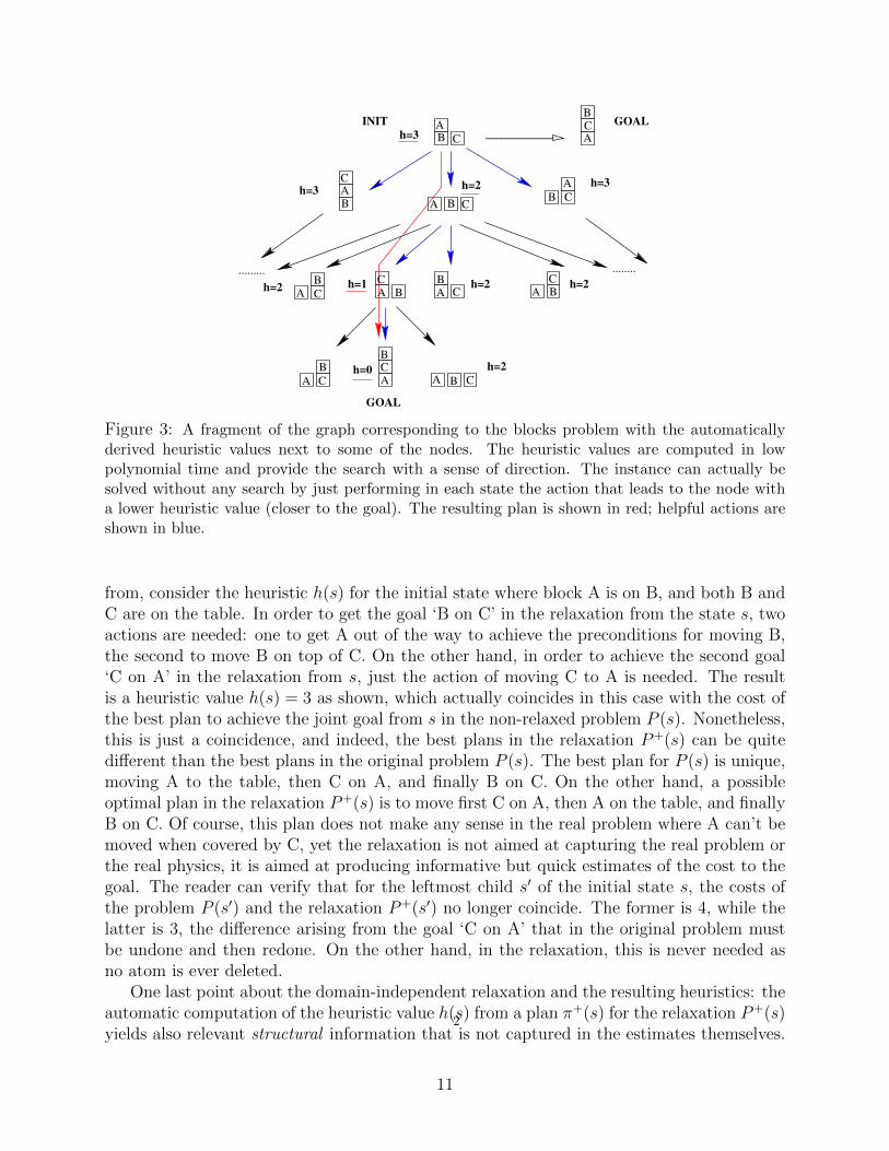
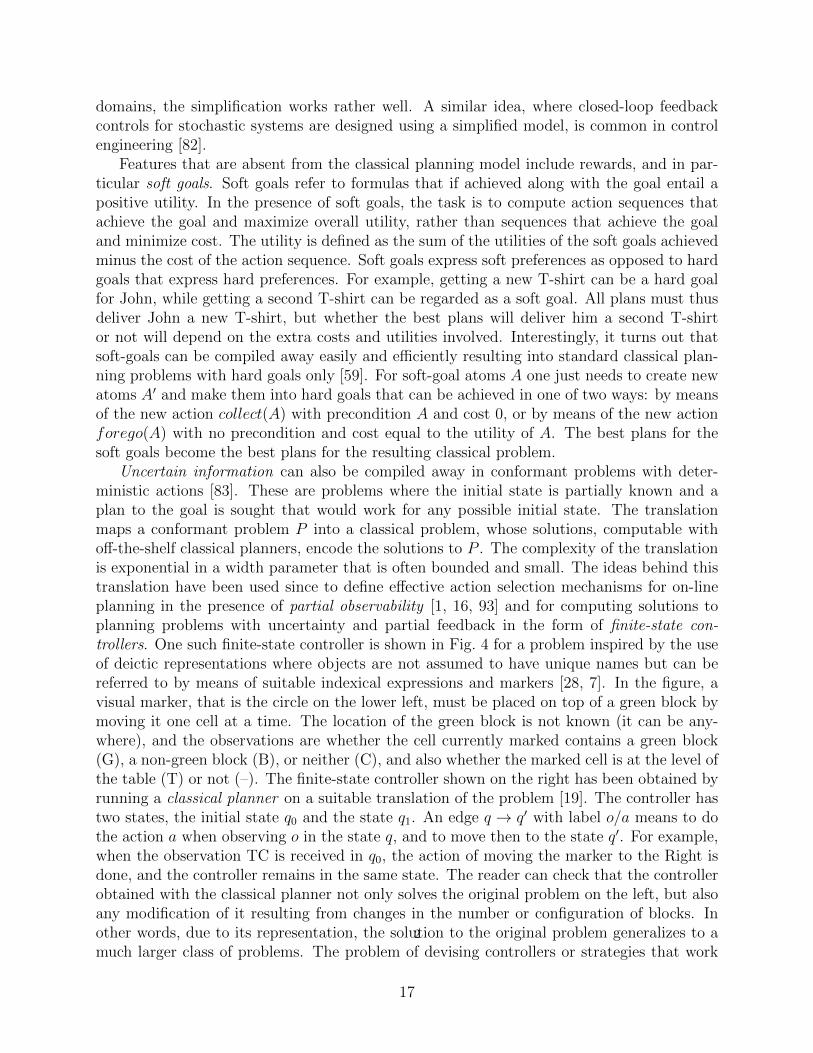
Uncertain information can also be compiled away in conformant problems with deter-ministic actions [83]. These are problems where the initial state is partially known and aplan to the goal is sought that would work for any possible initial state. The translationmaps a conformant problem P into a classical problem, whose solutions, computable withoff-the-shelf classical planners, encode the solutions to P . The complexity of the translationis exponential in a width parameter that is often bounded and small. The ideas behind thistranslation have been used since to define effective action selection mechanisms for on-lineplanning in the presence of partial observability [1, 16, 93] and for computing solutions toplanning problems with uncertainty and partial feedback in the form of finite-state con-trollers. One such finite-state controller is shown in Fig. 4 for a problem inspired by the useof deictic representations where objects are not assumed to have unique names but can bereferred to by means of suitable indexical expressions and markers [28, 7]. In the figure, avisual marker, that is the circle on the lower left, must be placed on top of a green block bymoving it one cell at a time. The location of the green block is not known (it can be any-where), and the observations are whether the cell currently marked contains a green block(G), a non-green block (B), or neither (C), and also whether the marked cell is at the level ofthe table (T) or not (–). The finite-state controller shown on the right has been obtained byrunning a classical planner on a suitable translation of the problem [19]. The controller hastwo states, the initial state q0 and the state q1. An edge q → q′ with label o/a means to dothe action a when observing o in the state q, and to move then to the state q′. For example,when the observation TC is received in q0, the action of moving the marker to the Right isdone, and the controller remains in the same state. The reader can check that the controllerobtained with the classical planner not only solves the original problem on the left, but alsoany modification of it resulting from changes in the number or configuration of blocks. Inother words, due to its representation, the solution to the original problem generalizes to amuch larger class of problems. The problem of devising controllers or strategies that work

17

2

q0

TB/Up

-B/Up

TC/Right

q1-C/Down

TB/Right

-B/Down

Figure 4: Left: Problem where visual-marker (circle on the lower left) must be placed on top of a greenblock by just observing what’s on the marked cell. Right: Finite-state controller obtained with a classicalplanner from suitable translation. The controller has two states, the initial state q0 and the state q1. Anedge q → q′ with label o/a means to do the action a when observing o in the state q, and to move then tothe state q′. The controller shown solves the problem, and any variation of it resulting from changes in thenumber or configuration of blocks.

for many or even all domain instances is usually referred to as generalized planning [70, 51].

11 Challenges

There are several open challenges in planning research. One of them is planning in thepresence of other agents that plan, often called multiagent planning. People do this naturallyall the time: walking on the street, driving, etc. The first question is how plans should bedefined. This is a subtle problem and many proposals have been put forward, often buildingon equilibria notions from game theory [22, 66, 23]. Yet, there are currently no models,algorithms, or implementations of domain-independent planners able to plan meaningfullyand efficiently in such settings. This is not entirely surprising, however, given the knownlimitations of game theory as a descriptive theory of human behavior [27]. Eventually, aworking theory of multiagent planning could shed light on the computation, nature, androle of social emotions in multiagent settings, very much as single-agent planning may shedlight on the computation, nature, and role of goal appraisals and heuristics in the single-agent setting. A second open problem is the automatic construction and use of hierarchies.Hierarchies form a basic component of Hierarchical Task Networks or HTNs, an alternativemodel for planning that is concerned with the encoding of strategies for solving problems[99, 34, 39], yet hierarchies play no role in state-of-the-art domain independent plannerswhich are completely flat. There is a large body of work on abstract problem solving thatis relevant to this question, both old [90, 63, 60, 5] and new [76, 69, 52], but no robustanswer yet. A third open problem is learning the planning models by interacting with theenvironment. We have discussed model-based reinforcement learning algorithms that activelylearn model parameters such as probabilities and rewards [56, 24, 2], yet a harder problemis learning the states themselves from partial observations. Several attempts to generalizereinforcement learning algorithms to partially observable settings have been made, some ofwhich learn to identify useful features and feature histories [73, 96, 102], but none so far thatcan come up with the states and models themselves in a robust and scalable manner.

18

2

12 Discussion

The relevance of the early work in AI to Cognitive Science was based on intuition: programsprovided a way for specifying intuitions precisely and for trying them out. The more recentwork on domain-independent solvers in AI is more technical and experimental, and is focusednot on reproducing intuitions but on scalability. This may give the impression that recentwork in AI is less relevant to Cognitive Science than work in the past. This impression,however, may prove wrong on at least two grounds. First, intuition is not what it used tobe, and it is now regarded as the tip of an iceberg whose bulk is made of massive amountsof shallow, fast, but unconscious inference mechanisms that cannot be rendered explicit[104, 47, 40]. Second, whatever these mechanisms are, they appear to work pretty well andto scale up. This is no small feat, given that most methods, whether intuitive or not, donot. By focusing on the study of meaningful models and the computational methods fordealing with them effectively, AI may prove its relevance to the understanding of humancognition in ways that may go well beyond the rules, cognitive architectures, and knowledgestructures of the 80’s. Human cognition, indeed, still provides the inspiration and motivationfor a lot of research in AI. The use of Bayesian networks in developmental psychology forunderstanding how children acquire and use causal relations [42], and the use of reinforcementlearning algorithms in neuroscience for interpreting the activity of dopamine cells in the brain[92], are two examples of general AI techniques that have made it recently into cognitivescience. As AI focuses on models and solvers able to scale up, more techniques are likely tofollow. In this paper, we have reviewed work in computational models of planning in AI,with an emphasis on deterministic planning models where automatically derived relaxationsand heuristics manage to integrate information about the current situation, the goal, andthe actions for directing the agent effectively towards the goal. The computational model ofgoal appraisals that is based on the solution of low-polynomial relaxations may shed lighton the computation, nature, and role of other types of appraisals, and on why appraisals areopaque to cognition and cannot be rendered conscious or articulated in words.

Acknowledgments.

The author thanks the reviewers for useful comments. H. Geffner is partially supportedby grants TIN2009-10232 and CSD2010-00034 (SimulPast), MICINN, Spain, and EC-7PM-SpaceBook.

References

[1] A. Albore, H. Palacios, and H. Geffner. A translation-based approach to contingentplanning. In Proc. IJCAI-09, pages 1623–1628, 2009.

[2] J. Asmuth and M. Littman. Learning is planning: near bayes-optimal reinforcementlearning via Monte-Carlo tree search. In Proc. UAI, pages 19–26, 2011.

[3] K. Astrom. Optimal control of markov decision processes with incomplete state esti-mation. J. Math. Anal. Appl., 10:174–205, 1965.

19

2

[4] H. Attias. Planning by probabilistic inference. In Proc. of the 9th Int. Workshop onArtificial Intelligence and Statistics, 2003.

[5] F. Bacchus and Q. Yang. Downward refinement and the efficiency of hierarchicalproblem solving. Artificial Intelligence, 71:43–100, 1994.

[6] C. Backstrom and B. Nebel. Complexity results for SAS+ planning. ComputationalIntelligence, 11(4):625–655, 1995.

[7] D. Ballard, M. Hayhoe, P. Pook, and R. Rao. Deictic codes for the embodiment ofcognition. Behavioral and Brain Sciences, 20(4):723–742, 1997.

[8] A. Barto, S. Bradtke, and S. Singh. Learning to act using real-time dynamic program-ming. Artificial Intelligence, 72:81–138, 1995.

[9] R. Bellman. Dynamic Programming. Princeton University Press, 1957.

[10] D. Bertsekas. Dynamic Programming and Optimal Control, Vols 1 and 2. AthenaScientific, 1995.

[11] A. Biere, M. Heule, H. van Maaren, and T. Walsh, editors. Handbook of Satisfiability:Volume 185 Frontiers in Artificial Intelligence and Applications. IOS Press, 2009.

[12] A. Blum and M. Furst. Fast planning through planning graph analysis. In Proceedingsof IJCAI-95, pages 1636–1642. Morgan Kaufmann, 1995.

[13] B. Bonet and H. Geffner. Planning as heuristic search. Artificial Intelligence, 129(1–2):5–33, 2001.

[14] B. Bonet and H. Geffner. Labeled RTDP: Improving the convergence of real-timedynamic programming. In Proc. 13th Int. Conf. on Automated Planning and Scheduling(ICAPS-2003), pages 12–31. AAAI Press, 2003.

[15] B. Bonet and H. Geffner. Solving POMDPs: RTDP-Bel vs. point-based algorithms.In Proc. IJCAI, pages 1641–1646, 2009.

[16] B. Bonet and H. Geffner. Planning under partial observability by classical replanning:Theory and experiments. In Proc. IJCAI-11, pages 1936–1941, 2011.

[17] B. Bonet and H. Geffner. Action selection for MDPs: Anytime AO* vs. UCT. In Proc.AAAI-2012, 2012.

[18] B. Bonet, G. Loerincs, and H. Geffner. A robust and fast action selection mechanismfor planning. In Proc. AAAI-97, pages 714–719, 1997.

[19] B. Bonet, H. Palacios, and H. Geffner. Automatic derivation of memoryless policiesand finite-state controllers using classical planners. In Proc. ICAPS-09, pages 34–41,2009.

20

2

[20] M. Botvinick and J. An. Goal-directed decision making in the prefrontal cortex: a com-putational framework. Advances in Neural Information Processing Systems (NIPS),pages 169–176, 2008.

[21] C. Boutilier, T. Dean, and S. Hanks. Decision-theoretic planning: Structural assump-tions and computational leverage. J. Artif. Intell. Res. (JAIR), 11:1–94, 1999.

[22] M. Bowling, R. Jensen, and M. Veloso. A formalization of equilibria for multiagentplanning. In Proc. IJCAI-03, pages 1460–1462, 2003.

[23] R. Brafman, C. Domshlak, Y. Engel, and M. Tennenholtz. Planning Games. In Proc.IJCAI-09, pages 73–78, 2009.

[24] R. Brafman and M. Tennenholtz. R-Max: A general polynomial time algorithm fornear-optimal reinforcement learning. Journal of Machine Learning Research, 3:213–231, 2003.

[25] R. Brooks. A robust layered control system for a mobile robot. IEEE J. of Roboticsand Automation, 2:14–27, 1987.

[26] T. Bylander. The computational complexity of STRIPS planning. Artificial Intelli-gence, 69:165–204, 1994.

[27] C. Camerer. Behavioral game theory: Experiments in strategic interaction. PrincetonUniversity Press, 2003.

[28] D. Chapman. Penguins can make cake. AI magazine, 10(4):45–50, 1989.

[29] A. J. Coles, A. Coles, A. G. Olaya, S. Jimenez, C. L. Lopez, S. Sanner, and S. Yoon. Asurvey of the seventh international planning competition. AI Magazine, 33(1):83–88,2012.

[30] T. H. Cormen, C. E. Leiserson, R. L. Rivest, and C. Stein. Introduction to Algorithms.The MIT Press, 2009.

[31] A. Damasio. Descartes’ Error: Emotion, Reason, and the Human Brain. Quill, 1995.

[32] D. Dennett. Kinds of minds. Basic Books New York, 1996.

[33] E. Dijkstra. A note on two problems in connexion with graphs. Numerische mathe-matik, 1(1):269–271.

[34] K. Erol, J. Hendler, and D. S. Nau. HTN planning: Complexity and expressivity. InProc. AAAI-94, pages 1123–1123, 1994.

[35] R. Fikes and N. Nilsson. STRIPS: A new approach to the application of theoremproving to problem solving. Artificial Intelligence, 1:27–120, 1971.

[36] H. Geffner. Heuristics, planning, cognition. In R. Dechter, H. Geffner, and J. Halpern,editors, Heuristics, Probability and Causality. A Tribute to Judea Pearl. College Pub-lications, 2010.

21

2

[37] H. Geffner and B. Bonet Advanced Introduction to Planning: Models and Methods.Morgan & Claypool. May 2013.

[38] S. Gelly and D. Silver. Combining online and offline knowledge in UCT. In Proc.ICML, pages 273–280, 2007.

[39] M. Ghallab, D. Nau, and P. Traverso. Automated Planning: theory and practice.Morgan Kaufmann, 2004.

[40] G. Gigerenzer. Gut feelings: The intelligence of the unconscious. Viking Books, 2007.

[41] G. Gigerenzer and P. Todd. Simple Heuristics that Make Us Smart. Oxford, 1999.

[42] A. Gopnik, C. Glymour, D. Sobel, L. Schulz, T. Kushnir, and D. Danks. A theoryof causal learning in children: Causal maps and Bayes nets. Psychological Review,111(1):3–31, 2004.

[43] J. Gratch. Why you should buy an emotional planner. In Proc. ofAgents’99 Workshop on Emotion-based Agent Architectures (EBAA’99), 1999. Athttp://emotions.usc.edu/∼gratch/gratch-ebaa99.pdf.

[44] J. Gratch and S. Marsella. A domain-independent framework for modeling emotion.Cognitive Systems Research, 5(4):269–306, 2004.

[45] P. Hart, N. Nilsson, and B. Raphael. A formal basis for the heuristic determination ofminimum cost paths. IEEE Trans. Syst. Sci. Cybern., 4:100–107, 1968.

[46] P. Haslum and H. Geffner. Admissible heuristics for optimal planning. In Proc. of theFifth International Conference on AI Planning Systems (AIPS-2000), pages 70–82,2000.

[47] R. Hassin, J. Uleman, and J. Bargh. The new unconscious. Oxford University Press,2005.

[48] J. Hoffmann and B. Nebel. The FF planning system: Fast plan generation throughheuristic search. Journal of Artificial Intelligence Research, 14:253–302, 2001.

[49] J. Hoffmann, J. Porteous, and L. Sebastia. Ordered landmarks in planning. Journalof Artificial Intelligence Research, 22:215–278, 2004.

[50] R. Howard. Dynamic Probabilistic Systems–Volume I: Markov Models. Wiley, NewYork, 1971.

[51] Y. Hu and G. De Giacomo. Generalized planning: Synthesizing plans that work formultiple environments. In Proc. IJCAI, pages 918–923, 2011.

[52] A. Jonsson. The role of macros in tractable planning over causal graphs. In Proc.IJCAI-07, pages 1936–1941, 2007.

22

2

[53] L. Kaelbling, M. Littman, and T. Cassandra. Planning and acting in partially observ-able stochastic domains. Artificial Intelligence, 101(1–2):99–134, 1998.

[54] D. Kahneman. Thinking, fast and slow. Farrar, Straus and Giroux, 2011.

[55] H. Kautz and B. Selman. Pushing the envelope: planning, propositional logic, andstochastic search. In Proc. AAAI, pages 1194–1201, 1996.

[56] M. Kearns and S. Singh. Near-optimal reinforcement learning in polynomial time.Machine Learning, 49(2):209–232, 2002.

[57] T. Keller and P. Eyerich. PROST: Probabilistic planning based on UCT. In Proc.ICAPS, 2012.

[58] E. Keyder and H. Geffner. Heuristics for planning with action costs revisited. In Proc.ECAI-08, pages 588–592, 2008.

[59] E. Keyder and H. Geffner. Soft goals can be compiled away. Journal of ArtificialIntelligence Research, 36:547–556, 2009.

[60] C. Knoblock. Learning abstraction hierarchies for problem solving. In Proc. AAAI-90,pages 923–928, 1990.

[61] L. Kocsis and C. Szepesvari. Bandit based Monte-Carlo planning. In Proc. ECML-2006, pages 282–293, 2006.

[62] A. Kolobov, Mausam, and D. Weld. LRTDP vs. UCT for online probabilistic planning.In Proc. AAAI, 2012.

[63] R. Korf. Planning as search: A quantitative approach. Artificial Intelligence, 33(1):65–88, 1987.

[64] R. Korf. Real-time heuristic search. Artificial Intelligence, 42:189–211, 1990.

[65] R. Korf. Finding optimal solutions to Rubik’s cube using pattern databases. In Proc.AAAI-98, pages 1202–1207, 1998.

[66] R. Larbi, S. Konieczny, and P. Marquis. Extending classical planning to the multi-agent case: A game-theoretic approach. In Proc. 9th European Conf. on Symbolic andQuantitative Approaches to Reasoning with Uncertainty (ECSQARU 2007), volume4724 of Lecture Notes in Computer Science, pages 731–742. Springer, 2007.

[67] N. Lipovetzky and H. Geffner. Width and serialization of classical planning problems.In Proc. ECAI, pages 540–545. IOS Press, 2012.

[68] A. Martelli and U. Montanari. Additive AND/OR graphs. In Proc. IJCAI-73, pages1–11, 1973.

[69] B. Marthi, S. Russell, and J. Wolfe. Angelic semantics for high-level actions. In Proc.ICAPS-07, pages 232–239, 2007.

23

2

[70] M. Martin and H. Geffner. Learning generalized policies from planning examples usingconcept languages. Appl. Intelligence, 20(1):9–19, 2004.

[71] M. J. Mataric. The Robotics Primer. MIT Press, 2007.

[72] D. McAllester and D. Rosenblitt. Systematic nonlinear planning. In Proceedings ofAAAI-91, pages 634–639, 1991.

[73] A. McCallum. Overcoming incomplete perception with utile distinction memory. InProceedings Tenth Int. Conf. on Machine Learning, pages 190–196, 1993.

[74] D. McDermott. A heuristic estimator for means-ends analysis in planning. In Proc.AIPS-96, pages 142–149, 1996.

[75] D. McDermott. PDDL – the planning domain definition language. Athttp://ftp.cs.yale.edu/pub/mcdermott, 1998.

[76] S. McIlraith and R. Fadel. Planning with complex actions. In Proc. NMR-02, pages356–364, 2002.

[77] M. Minsky. Steps toward artificial intelligence. Proceedings of the IRE, 49(1):8–30,1961.

[78] T. Mitchell. Machine Learning. McGraw-Hill, 1997.

[79] A. Newell, J. C. Shaw, and H. Simon. Chess-playing programs and the problem ofcomplexity. In E. Feigenbaum and J. Feldman, editors, Computers and Thought, pages109–133. McGraw Hill, 1963.

[80] A. Newell and H. Simon. Elements of a theory of human problem solving. PsychologyReview, 1958.

[81] A. Newell and H. Simon. GPS: a program that simulates human thought. In E. Feigen-baum and J. Feldman, editors, Computers and Thought, pages 279–293. McGraw Hill,1963.

[82] K. Ogata. Modern control engineering. Prentice Hall, 2001.

[83] H. Palacios and H. Geffner. Compiling Uncertainty Away in Conformant PlanningProblems with Bounded Width. Journal of Artificial Intelligence Research, 35:623–675, 2009.

[84] J. Pearl. Heuristics. Addison Wesley, 1983.

[85] J. Penberthy and D. Weld. UCPOP: A sound, complete, partiall order planner forADL. In Proc. KR-92, 1992.

[86] M. Puterman. Markov Decision Processes – Discrete Stochastic Dynamic Program-ming. John Wiley and Sons, Inc., 1994.

24

2

[87] S. Richter and M. Westphal. The LAMA planner: Guiding cost-based anytime planningwith landmarks. Journal of Artificial Intelligence Research, 39(1):127–177, 2010.

[88] J. Rintanen. Heuristics for planning with SAT. In Proc. on Principles and Practice ofConstraint Programming (CP 2010), pages 414–428. Springer, 2010.

[89] S. Russell and P. Norvig. Artificial Intelligence: A Modern Approach. Prentice Hall,2009. 3rd Edition.

[90] E. Sacerdoti. Planning in a hierarchy of abstraction spaces. Artificial intelligence,5(2):115–135, 1974.

[91] E. Sacerdoti. The nonlinear nature of plans. In Proc. IJCAI-75, pages 206–214, 1975.

[92] W. Schultz, P. Dayan, and P. Montague. A neural substrate of prediction and reward.Science, 275(5306):1593–1599, 1997.

[93] G. Shani and R. Brafman. Replanning in domains with partial information and sensingactions. In Proc. IJCAI-2011, pages 2021–2026, 2011.

[94] D. Silver and J. Veness. Monte-Carlo planning in large POMDPs. In Advances inNeural Information Processing Systems (NIPS), pages 2164–2172, 2010.

[95] H. Simon. A behavioral model of rational choice. The quarterly journal of economics,69(1):99–118, 1955.

[96] K. Stanley, B. Bryant, and R. Miikkulainen. Real-time neuroevolution in the nerovideo game. Evolutionary Computation, IEEE Transactions on, 9(6):653–668, 2005.

[97] R. Sutton. Learning to predict by the methods of temporal differences. Machinelearning, 3(1):9–44, 1988.

[98] R. Sutton and A. Barto. Introduction to Reinforcement Learning. MIT Press, 1998.

[99] A. Tate. Generating project networks. In Proc. IJCAI, pages 888–893, 1977.

[100] J. Tooby and L. Cosmides. The psychological foundations of culture. In J. Barkow,L. Cosmides, and J. Tooby, editors, The Adapted Mind. Oxford, 1992.

[101] M. Toussaint and A. Storkey. Probabilistic inference for solving discrete and continuousstate markov decision processes. In Proc. 23rd Int. Conf. on Machine Learning, pages945–952, 2006.

[102] J. Veness, K. Ng, M. Hutter, W. Uther, and D. Silver. A Monte-Carlo AIXI approxi-mation. Journal of Artificial Intelligence Research, 40(1):95–142, 2011.

[103] C. Watkins and P. Dayan. Q-learning. Machine learning, 8(3):279–292, 1992.

[104] T. Wilson. Strangers to ourselves. Belknap Press, 2002.

25

2

[105] S. Yoon, A. Fern, and R. Givan. FF-replan: A baseline for probabilistic planning. InProc. ICAPS-07, pages 352–359, 2007.

[106] H. Younes, M. Littman, D. Weissman, and J. Asmuth. The first probabilistic trackof the international planning competition. Journal of Artificial Intelligence Research,24:851–887, 2005.

26