computational methods in machine learning: transport … · we deﬁne the transport operator, t,...

OverviewIntroduction

Transport by advectionExperiments and results

COMPUTATIONAL METHODS IN MACHINE LEARNING:TRANSPORT MODEL, HAAR WAVELET,

DNA CLASSIFICATION, AND MRI

Franck Olivier Ndjakou Njeunje

Applied Mathematics, Statistics, and Scientific ComputationNorbert Wiener Center

Department of MathematicsUniversity of Maryland, College Park



Outline

1 Overview

2 Introduction

3 Transport by advection

4 Experiments and results



Overview

My dissertation includes the following topics:

Haar approximation from within for Lp(Rd), 0 < p < 1

Theorem (J. Benedetto and F. Njeunje)

Let f ∈ Lp(R), where 0 < p < 1 suppose f is a continuous function on R, withsupp f ⊆ [A,B]. Then, for all ε > 0, there is an M = M(ε), and there is asequence of sums,

fM,k =∑

(i,j)∈SM,k

ai,j ψi,j , ai,j ∈ C,

indexed by k ≥ 1, where SM,k ⊆ Z× Z and card SM,k <∞, with the followingproperties:

if (i , j) ∈ SM,k then supp ψi,j ⊆ supp f ,

and∃K = K (ε) such that ∀k > K , ‖f − fM,k‖p < ε.



Overview

My dissertation includes the following topics:

Classification of multiton enhancersIn collaboration with Dr. Ivan Ovcharenko and his research group at theNational Institutes of Health (NIH).Enhancers are particular deoxyribonucleic acid (DNA) segments thatincrease or enhance the likelihood of gene expression.Singletons vs. multitons.We constructed a classifier using support vector machine to identifymultitons having similar characteristics to singletons with high probability.

Analysis of T2-store-T2 magnetic resonance relaxometry with Nexchanging sites

In collaboration with Dr. Richard G. Spencer and his research group at NIH.Magnetic resonance imaging (MRI) is a tool used for diagnosing anatomyand pathology, including osteoarthritis.We successfully extended the analysis of the magnetization signal from 2sites to N sites.

Transport operator on graphIn collaboration with Prof. Wojciech Czaja and Prof. Pierre-Emmanuel Jabin.This presentation contains material from this topic.



Outline

1 Overview

2 Introduction





Introduction

The curse of dimensionalityThis expression was coined by Richard Bellman and refers to the problemcaused by the exponential increase in volume associated with adding extradimensions to a mathematical space.In data science this means that the number of observations needed to obtainfavorable results grows exponentially with the number of dimensions.

Dimension reduction (DR):Principal component analysis (PCA), by Pearson1.

Based on the covariance matrix.Search of the orthogonal directions of greatest variance explaining as much ofthe data as possible.

Kernel PCA, by Scholkopf2.Non-linear adaptation of PCA.A great number of non-linear DR algorithms are special cases of kernel PCA.

1K. Pearson, On lines and planes of closest fit to systems of point in space, Philosophical Magazine 2 (1901), no. 11, 559-572.2B. Scholkopf, A. Smola, and K-R. Muller, Kernel principal component analysis, International Conference on Artificial Neural Networks,

Springer, 1997, pp. 583-588.



Introduction

Dimension reduction (DR):Diffusion maps (DIF), by Coifman and Lafon3.

Diffusion maps are constructed using eigenfunctions of Markov matrices.They generate efficient representations of complex geometric structures.

Isomap (ISO), by Tenenbaum4.Based on the geodesic distance between points measured along the manifold.

Laplacian eigenmaps (LE), by Belkin and Niyogi5.Preserves local information embedded in low dimensional manifold.

Schroedinger eigenmaps (SE), by Czaja and Ehler6.Semi-supervised generalization of LE.Uses barrier potential to stir the diffusion process.

3R. R. Coifman and S. Lafon, Diffusion maps, Applied and Computational Harmonic Analysis 21 (2006), no. 1, 5-30.4J. B. Tenenbaum, V. De Silva, and J. C. Langford, A global geometric framework for nonlinear dimensionality reduction, Science 290

(2000), no. 5500, 2319-2323.5M. Belkin and P. Niyogi, Laplacian eigenmaps and spectral techniques for embedding and clustering, Advances in Neural Information

Processing Systems, 2002, pp. 585-591.6W. Czaja and M. Ehler, Schroedinger eigenmaps for the analysis of biomedical data, IEEE Transactions on Pattern Analysis and

Machine Intelligence 35 (2013), no. 5, 1274-1280.



Laplacian eigenmaps: optimization problem

Given a set of n points X = {x1, x2, . . . , xn} in Rd , the goal is to find anoptimal embedding for these points in a lower m-dimensional space wherem� d , while preserving local information.

The embedding is given by the n ×m matrix Y = [y1, y2, . . . , ym], where thei th row corresponds to the embedded coordinates of the i th points xi . Theobjective to the minimization problem7 is written as∑

i,j

‖y(i) − y(j)‖2wij = tr (YT LY), (1)

where

y(i) = [y1(i), . . . , ym(i)]T is the m-dimensional representation of the i th

point xi .

With the appropriate choice of weights wij , minimizing (1) ensures thatadjacent points remain close together after the mapping.

7M. Belkin and P. Niyogi, Laplacian eigenmaps for dimensionality reduction and data representation, Neural Computation 15 (2003),no. 6, 1373-1396.



Laplacian eigenmaps: algorithm

The LE algorithm we will be using in our work involves the following steps:

Step 1: Construct the adjacency graph using the k -nearest neighbor(kNN) algorithm. This is done by putting an edge connecting nodes i andj given that xi is among the k nearest neighbors of xj .

Step 2: Define a graph Laplacian, L , using the weight matrix, W . Theweights in W are chosen using the heat kernel with parameter σ. Ifnodes i and j are connected,

wij = exp

(−‖xi − xj‖2

2σ2

);

otherwise, wij = 0. The graph Laplacian is given by

L = D −W ,

where D is a diagonal matrix with entries dii =∑

i wij .



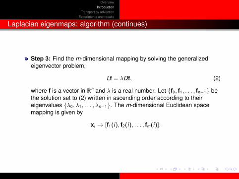
Laplacian eigenmaps: algorithm (continues)

Step 3: Find the m-dimensional mapping by solving the generalizedeigenvector problem,

Lf = λDf, (2)

where f is a vector in Rn and λ is a real number. Let {f0, f1, . . . , fn−1} bethe solution set to (2) written in ascending order according to theireigenvalues {λ0, λ1, . . . , λn−1}. The m-dimensional Euclidean spacemapping is given by

xi → [f1(i), f2(i), . . . , fm(i)].



Example: LE vs PCA

Laplacian eigenmaps is able to represent the data in a reasonablemanner preserving local information.PCA fails to capture the true nature of the data and simply project it to a2-dimensional space.

Figure 1: The leftmost plot represents a set of 2000 3-dimensional points sitting on a swiss roll;the middle plot represents the embedding in 2-dimension using principal component analysis(PCA); and the rightmost plot represents the same embedding using Laplacian eigenmaps (LE)with k = 12 (number of neighbors per node) and σ = 1.



Schroedinger eigenmaps: optimization problem

Czaja and Ehler proposed the Schroedinger eigenmaps (SE) algorithm:

Semi-supervised generalization to the LE algorithm using partialknowledge about the ground truth of the data set.

The minimization problem8

minYT DY=I

12

∑i,j

‖y(i) − y(j)‖2wij + α∑

i

V (i)‖y(i)‖2, (3)

where V is the diagonal matrix with entries V (1) through V (n).

The second component of the sum (3) add an extra level of clustering onthe representation y(i) which are associated with large value of V (i).

Partial knowledge about the data is used to build barrier potential,encoded in the matrix V , to stir the diffusion process in order to obtainsuitable results

8W. Czaja and M. Ehler, Schroedinger eigenmaps for the analysis of biomedical data, IEEE Transactions on Pattern Analysis andMachine Intelligence 35 (2013), no. 5, 1274-1280.



Schroedinger eigenmaps: algorithm

Given a set of n points X = {x1, x2, . . . , xn} in Rd and a function µ,

µ : X → R,

containing the extra information over the set of points X , the SE algorithm wewill be using in our work involves the following steps:

Step 1: Construct the adjacency graph.Step 2: Define a graph Laplacian, L, using the weight matrix, W .Step 3: Define the Schrodinger matrix, S, using the extra information, µ.

S = L + αV ,

where α is a real number, and V is the diagonal potential matrix given by

V =

µ1

µ2

. . .µn

, (4)

where µi = µ(xi) for all i = 1, . . . , n.



Schroedinger eigenmaps: algorithm (continues)


Sf = λDf, (5)


xi → [f1(i), f2(i), . . . , fm(i)].



Outline

1 Overview

2 Introduction





Continuous model: notations

We consider a graph as a set of points X = {x1, x2, . . . , xn} in Rd , orequivalently as a set of indices i in I = {1, 2, . . . , n}.

We denote Ai as the set of adjacent indices to i

We denote A = {(i , j) : j ∈ Ai} as the set of edges of the graph

We denote P as the set of probability distributions µ from I to R+, µ issuch that

µ ∈ P ⇒∑

i

µi = 1.

We denote E as the set of functions from A to R, and

We denote Ea as the set of functions v in E that are antisymmetric, that is

vij = −vji .



Continuous model: definition

Let µ ∈ P, and v ∈ Ea a velocity field that is itself a function of µ. Thetransport model we consider is also known as the transport by advection; itrefers to the active transportation of a distribution, µ, by a flow field, v .

We define the transport operator, T , acting on µ as follows:

Tµ = 4µ− div(vµ). (6)

4 denotes the Laplacian defined as the divergence of the gradient acting on a distribution µ.

div denotes the divergence, a vector operator that produces a scalar field quantifying a vectorfield’s source at each point.

We denote∇ as the gradient acting on a scalar field.

A comprehensive study of the operator in (6) is found in related materials by Benamou et al.9

and Hundsdorfer et al.10.

Given an appropriately chosen flow field, v , we are able to direct the diffusion process inorder to form desirable clusters.

9J-D. Benamou, B. D. Froese, and A. M. Oberman, Numerical solution of the optimal transportation problem using the Monge-Ampeereequation, Journal of Computational Physics 260 (2014), 107-126.

10W. Hundsdorfer and J. G. Verwer, Numerical solution of time-dependent advection-diffusion-reaction equations, vol. 33, SpringerScience & Business Media, 2013.



Discrete model: discretization

We propose the following discretization as well as matrix formulation:

Given a function µ on I, we define the gradient of µ as ∇µ by

(∇µ)ij = wij(µj − µi).

We also define the Laplacian of µ as 4µ = div(∇µ) by

(4µ)i =∑j∈Ai

wij(µj − µi).

The centered discretization of vµ is given by:

(vµ)cij = vij

µi + µj

2.

Our choice of discretization schemes is motivated by its well-defined analyticproperties.



Discrete model and derivative

We consider a purely local type of flow by taking v = β∇µ, where β is a realnumber. Using the central discretization, we obtain the following equation:

(Tµ)i =∑j∈Ai

wij(µj − µi)− β∑j∈Ai

wij(µ2j − µ2

i ), for each i ∈ I

= (Fl(µ))i − β(Fd(µ))i , for each i ∈ I.

The derivatives of Fl and Fd with respect to µ are:

F ′l (µ) = L and F ′d(µ) = 2Cµ ◦ L,

where the operation ◦ is the element-wise multiplication, and the matrix Cµ isgiven by

Cµ =

...

......

...µ1 µ2 . . . µn...

......

...

.



Linearization

We finally write the linearization, T , of the transport operator around anygiven distribution µ as

T (u) = [L− 2βCµ ◦ L](u) ∀u ∈ P. (7)



Transport eigenmaps algorithm

Given a set of n points X = {x1, x2, . . . , xn} in Rd and a function µ

µ : X → R

over the set of points X . The transport eigenmaps algorithm involves thefollowing steps:

Step 1: Construct the adjacency graph.Step 2: Define a graph Laplacian, L, using the weight matrix, W .Step 3: Define the linearized transport matrix, T , using the extrainformation, µ.

T = L− 2βCµ ◦ L,

where β is a real number, the operation ◦ is the element-wisemultiplication and

Cµ =

...

......

...µ1 µ2 . . . µn...

......

...

, (8)

where µi = µ(xi) for all i = 1, . . . , n.



Transport eigenmaps algorithm (continues)


T f = λDf, (9)


xi → [f1(i), f2(i), . . . , fm(i)].



Outline

1 Overview

2 Introduction





Example: Laplacian, transport, and Schroedinger mapping

Figure 2: The first plot represents a set of points, 300 points grouped in 3 clusters of 100 pointseach, in the order blue, green, then yellow. The rest represents various mapping using the first andsecond eigenvectors with corresponding non-zero eigenvalue.



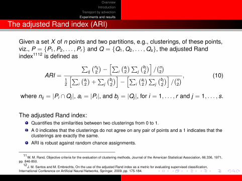
The adjusted Rand index (ARI)

Given a set X of n points and two partitions, e.g., clusterings, of these points,viz., P = {P1,P2, . . . ,Pr} and Q = {Q1,Q2, . . . ,Qs}, the adjusted Randindex1112 is defined as

ARI =

∑ij

(nij2

)−[∑

i

(ai2

)∑j

(bj2

)]/(n

2

)12

[∑i

(ai2

)+∑

j

(bj2

)]−[∑

i

(ai2

)∑j

(bj2

)]/(n

2

) , (10)

where nij = |Pi ∩Qj |, ai = |Pi |, and bj = |Qj |, for i = 1, . . . , r and j = 1, . . . , s.

The adjusted Rand index:Quantifies the similarities between two clusterings from 0 to 1.

A 0 indicates that the clusterings do not agree on any pair of points and a 1 indicates that theclusterings are exactly the same.

ARI is robust against random chance assignments.

11W. M. Rand, Objective criteria for the evaluation of clustering methods, Journal of the American Statistical Association, 66.336, 1971,pp. 846-850.

12J. M. Santos and M. Embrechts, On the use of the adjusted Rand index as a metric for evaluating supervised classification,International Conference on Artificial Neural Networks, Springer, 2009, pp. 175-184.



Representation experiment: setup

We demonstrate the strength of our algorithm in its ability to faithfullyrepresent the data using a large number of experiments.

Clusters are arranged in 2 or 3 dimensions increasing in difficulty.

We increase the difficulty by changing the parameters used to generatethe data set: position, spread or standard deviation, added Gaussiannoise, and number of clusters.

Example: changing the position

We use the adjusted Rand index (ARI) to quantify the representation ofthe data set.



Representation experiment: procedure

For each individual run, the following operations are performed:

Step 1: Generate the data set, X , and corresponding labels.

Step 2: We cluster the data set before and after dimension reductionusing the k-means algorithm.

Step 3: We compute the adjusted Rand index before and afterdimension reduction and store the difference.

The following dimension reduction algorithms are used in the experiment:

Principal components analysis (PCA),

Laplacian eigenmaps (LE),

Diffusion maps (DIF),

Isomap (ISO),

Schroedinger eigenmaps (SE),

Transport eigenmaps (TE).



Representation experiment: result - overall

A positive change in ARI implies a better representation of the data afterdimension reduction:

The rightmost position of the box plot corresponding to TE in relation tothe other DR algorithms implies that in general, TE produces the bestrepresentation of the data.

Figure 3: Box plot for the change of ARI, all 162× 20 = 3240 cases.



Representation experiment: result - complex and simple

The dominant performance of TE is more apparent on difficult cases, seeFigure 4, than it is on simple cases, see Figure 5.

Figure 4: Box plot for the change of adjusted Rand index, 126× 20 = 2520 difficult cases.

Figure 5: Box plot for the change of adjusted Rand index, 36× 20 = 720 simple cases.



Hyperspectral dataset: Indian Pines

In this section, we work with the Indian Pines1314 data set:Gathered by AVIRIS (Airborne Visible/Infrared Imaging Spectrometer) sensor.

Over the Indian Pines test site in North-western Indiana: 145× 145× 200.

Hyperspectral bands covering the region of water absorption have been removed.

Figure 6: Ground truth (left) and sample band: 170 (right.)

13M. F. Baumgardner, L. L. Biehl, and D. A. Landgrebe, 220 band AVIRIS hyperspectral image data set: June 12, 1992 Indian Pines testsite 3, September 2015.

14Hyperspectral remote sensing scenes, http://www.ehu.eus/ccwintco/index.php/Hyperspectral Remote Sensing Scenes, Accessed:2018-04-04.



Indian Pines: ground truth

# Class Sample0 Empty-space 107761 Alfalfa 462 Corn-notill 14283 Corn-mintill 8304 Corn 2375 Grass-pasture 4836 Grass-trees 7307 Grass-pasture-mowed 288 Hay-windrowed 4789 Oats 2010 Soybean-notill 97211 Soybean-mintill 245512 Soybean-clean 59313 Wheat 20514 Woods 126515 Buildings-Grass-Trees-Drives 38616 Stone-Steel-Towers 93

Table 1: Indian Pines classes.



Indian Pines grouped: ground truth

# Class Sample0 Empty-space 107761 Alfalfa 462 Corn 24955 Grass 12418 Hay-windrowed 4789 Oats 2010 Soybean 402013 Wheat 20514 Woods 126515 Buildings-Grass-Trees-Drives 38616 Stone-Steel-Towers 93

Table 2: Indian Pines-G classes, ground truth with corresponding grouped labels.



Extra information and parameters

Given prior knowledge about class 11–soybean-mintill in the IndianPines data set, we would place a potential for SE or an advection for TEon class 11–soybean-mintill using the function µ defined as follows:

µ(x) =

{1, if x ∈ Class 11–soybean-mintill,0, elsewhere.

We ran a set of experiments to obtain the following parameters:We set m = 50 (Indian Pines), k = 12, and σ = 1.We set β = 10 and α = 104, where the parameter α such thatα = α · tr (L)/tr (V ).



Classification and validation metric

After the embedding:We use the 1-nearest neighbor algorithm to classify the data sets.

We use 10% of the data from each class to train the classifier and the rest, Nv , as thevalidation set.

We took an average of ten runs to produce the confusion matrices, C.

We following validation metrics are reported:The adjusted Rand index (ARI) between the predicted labels and the ground truth.

The overall accuracy (OA).

The Cohen’s kappa coefficient1516 (κ) is defined by

κ =Nv

∑i (Ci,i )

2 − ωN2

v − ω,

where ω =∑

i Ci,·C·,i . Similar to ARI, κ measures the agreement between clusterings, a 0indicates no agreement while a 1 indicates complete agreement.

15Smeeton, N. C., Early history of the kappa statistic, 1985, pp. 795-795.16Galton, F, Finger Prints Macmillan, 1892.



Results: Indian Pines

The best representation and accuracy come from TE, with SE as a closesecond, see Table 3.

IP PCA LE DIF ISO SE-2 SE-11 TE-2 TE-11ARI 0.4426 0.3694 0.4210 0.3929 0.5520 0.6955 0.5735 0.7085OA 0.6761 0.6081 0.6556 0.6308 0.7138 0.7353 0.7281 0.7418κ 0.6301 0.5532 0.6065 0.5785 0.6732 0.6981 0.6900 0.7055

Table 3: Classification results for Indian Pines (IP).

Figure 7: Classification map.



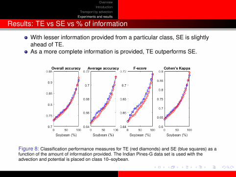
Results: TE vs SE vs % of information

With lesser information provided from a particular class, SE is slightlyahead of TE.As a more complete information is provided, TE outperforms SE.

Figure 8: Classification performance measures for TE (red diamonds) and SE (blue squares) as afunction of the amount of information provided. The Indian Pines-G data set is used with theadvection and potential is placed on class 10–soybean.



Results: robustness against noise

The added Gaussian noise has a mean of 0, we selected 20logarithmically spaced values for the standard deviation from 100 to 105.In general, TE is the most robust algorithm against noise.

Figure 9: TE (red diamonds), SE (blue boxes), PCA (green x’s), and LE (black circles). The IndianPines-G data set is used with the advection and potential is placed on class 10–soybean.



Conclusion

We constructed a novel semi-supervised non-linear dimension reductionalgorithm based on a transport model by advection.

We used advection, the active transportation of a distribution by a flowfield, to stir the diffusion process in order to get better or more desirableresults.

We provided a set of experiments based on artificially generated datasets and on publicly available hyperspectral data set to show that ouralgorithm exhibits superior/competitive performance.

We believe that the performance of our algorithm can be improved bychoosing alternative flow fields and/or using different linearizationtechniques.



Thank You!

computational methods in machine learning: transport … · we deﬁne the transport operator, t,...

Documents