laplacian damping for projective dynamics

Workshop on Virtual Reality Interaction and Physical Simulation VRIPHYS (2018)F. Jaillet, G. Zachmann, K. Erleben, and S. Andrews (Editors)

Laplacian Damping for Projective Dynamics

Jing Li1 Tiantian Liu2 Ladislav Kavan1

1University of Utah, United States2University of Pennsylvania, United States

AbstractDamping is an important ingredient in physics-based simulation of deformable objects. Recent work introduced new fast simu-lation methods such as Position Based Dynamics and Projective Dynamics. Explicit velocity damping methods currently usedin conjunction with Position Based Dynamics or Projective Dynamics are simple and fast, but have some limitations. They maydamp global motion or non-physically transport velocities throughout the simulated object. More advanced damping modelsdo not have these limitations, but are slow to evaluate, defeating the benefits of fast solvers such as Projective Dynamics. Wepresent a new type of damping model specifically designed for Projective Dynamics, which provides the quality of advanceddamping models while adding only minimal computing overhead. The key idea is to define damping forces using Projective Dy-namics’ Laplacian matrix. In a number of simulation examples we show that this damping model works very well in practice.When used with a modified Projective Dynamics solver that uses a non-dissipative implicit midpoint integrator, our dampingmethod provides fully user-controllable damping, allowing the user to quickly produce visually pleasing and vivid animations.

CCS Concepts• Computing methodologies → Physical simulation;

1. Introduction

Dissipation of mechanical energy is an important phenomenon innature. In computer animation, damping is used to enhance sta-bility of non-dissipative time integration schemes or to add aes-thetic control to the results of simulations. Explicit damping meth-ods produce fast damping effects, but may introduce unwanted ar-tifacts. Explicit damping can be as simple as reducing each ve-locity in the system by a fixed ratio. This method is known as“ether drag” [SSF13]. A limitation of the ether drag is that it dampsall velocities, even global rigid body motions. In order to miti-gate this problem, Position Based Dynamics introduced a damp-ing method (“PBD damping”) that modifies the vertex velocitieswithout changing the global motion, i.e. linear and angular mo-menta [MHHR07]. Even though this method successfully preservesthe linear and angular momenta, it can non-physically transport ve-locities throughout the object and make it appear unnaturally rigid,because the underlying idea is to factor out linear and angular ve-locities as in a rigid body simulation. Implicit damping methods,on the other hand, can produce more visually satisfying results, butwith extra computational cost.

Projective Dynamics [LBOK13,BML∗14,LBK17] is a fast time in-tegration method for elastic body simulations. Due to performanceconsiderations, only explicit damping methods were considered inProjective Dynamics so far. In this paper, we propose a fast implicitdamping method that can be naturally integrated into the frame-

work of Projective Dynamics with negligible extra computationalcost.

Our method is inspired by Rayleigh damping, which is extensivelyused in computer graphics [CAP17] [LKSH08] [GMD13] [FM17].One feature of Rayleigh damping is that it is effective at remov-ing high-frequency vibrations because the stiffness matrix acts asa high-pass filter [Wil02]. We use the Laplacian matrix to approx-imate this stiffness matrix because the Laplacian matrix is also ahigh-pass filter [Zha04] [Tau95] The key advantage of using theLaplacian matrix is that it is constant – independent of the currentstate of the simulated system – unlike the stiffness matrix. There-fore, Laplacian Damping can be efficiently incorporated in the Pro-jective Dynamics framework with minimal computing overheads.

The original Projective Dynamics method is derived from back-ward Euler, also known as implicit Euler. Backward Euler is astrongly dissipative integrator, containing significant “built-in” nu-merical damping which is not user-controllable. We can combineProjective Dynamics with different time integrators, such as im-plicit midpoint. Implicit midpoint is non-dissipative and thereforecan produce nice vivid motion, however, it is not always stable forlarge time steps. Our new damping method can be combined withimplicit midpoint in the Projective Dynamics framework, produc-ing stable motion that is as vivid motion as the user desires.

In summary, the main contributions of our new damping modelare:

c© 2018 The Author(s)Eurographics Proceedings c© 2018 The Eurographics Association.

DOI: 10.2312/vriphys.20181065

http://www.eg.org

http://diglib.eg.org

http://dx.doi.org/10.2312/vriphys.20181065

Jing Li, Tiantian Liu, Ladislav Kavan / Laplacian Damping for Projective Dynamics

• Our method does not exhibit the artifacts of fast explicit dampingmethods such as ether drag or PBD damping [MHHR07].

• Our method produces similar visual results to implicit dampingmethods such as lagged Rayleigh damping [GS14] or variationaldamping [KYT∗06] while being much faster.• Our method is easy to implement and fully compatible with the

Projective Dynamics framework.• Our method adds only minimal computing overheads on top of

the underlying Projective Dynamics simulator.

2. Background and Related Work

Damping is commonly observed in nature. For purposes of numer-ical simulations, simple damping model, such as viscous damping,can be often assumed. Force corresponding to viscous damping canbe expressed as:

fd =−Dv (1)

where D is a positive semi-definite damping matrix, v is the veloc-ity of all particles in the simulated system, and fd is the resultingdamping force. D can be arbitrary, even time-dependent. The sim-plest choice of D is a constant scaled identity matrix: D := kdIwhere kd is a constant damping coefficient [TPBF87]. Unfortu-nately, this damping model will also dissipate rigid body motions,i.e., global translation and rotation. This issue can be resolved byusing a strain rate dependent damping matrix.

A special class of viscous damping methods is called Caugheydamping [CO65]. It is designed for controlling the strength ofdamping for different vibrating components with different frequen-cies separately. The damping force in the Caughey damping modelis still proportional to the velocity as described in Eq. 1, but thedamping matrix becomes:

DCaughey := Mp

∑i=1

(αi

[M−1K

]i−1)

(2)

where M is the mass matrix of the system, typically diagonallylumped; K is the stiffness matrix, i.e., the Hessian matrix of theelastic potential energy (or, equivalently, Jacobian of the elasticforces). In Eq. 2, αi controls the strength of damping for vibrationmodes with different frequencies and p is the number of vibrationmodes. When only modes with the smallest vibration frequenciesare considered, i.e. p = 2, the Caughey damping model reduces toits linear case known as Rayleigh damping [Ray96]:

DRayleigh := α1M+α2K (3)

Recently, Xu el al. [XB17] proposed an example based method thatcan converge DRayleigh towards DCaughey by adding user-defined ex-amples. This is essentially an artist-friendly way to approximate aCaughey damping matrix.

A common way to implement damping is by integrating damp-ing forces in a separate numerical integration step, which can beeither explicit or implicit [BMF05]. Ether drag [SSF13] is the mostbasic explicit damping method, which corresponds to multiplyingall velocities by a constant (potentially spatially varying). Althoughthis is very fast, ether drag shares a similar problem as [TPBF87] -even rigid body motions are damped, reducing both linear and an-gular momentum of a system. In order to fix this issue, Müller et

al. [MHHR07] used a momentum-preserving explicit damping inPosition Based Dynamics (PBD), which is almost as fast as etherdrag. However, as we demonstrate in Figure 2, the results can beimplausible in some cases due to non-physical transport of veloci-ties through the simulated object. In cases where visual plausibilityis more important than performance, implicit damping methods canbe used. Bridson et al. [BMF05] combined a half step of implicitdamping and another half step of explicit elastic force integration,producing highly realistic cloth simulation results. Kharevych etal. [KYT∗06] proposed a new variational damping method, alsoincorporated a separate implicit time integration step.

Time Integration is one of the core ingredients of physicallybased simulation. Given the current state consisting of positions xnand velocities vn, we need to predict the next state xn+1, vn+1 usingNewton’s second law of motion. Different time integration methodsuse different discrete estimates (quadratures) of the forces. Withoutdamping, many implicit time integration schemes can be generallyexpressed as the following optimization problem:

g(x) = 12h2 ||x−y||2M + c1E(c2x+ z) (4)

this is a generalization of Eq.3 in [LBK17], where h is the timestep size, ||x||2M = xTMx stands for the norm of x weighted by themass matrix, E(x) is the elastic energy evaluated at position x, andthe scalars c1, c2 and the vectors y, z are time-integrator-dependentconstants. For example, in backward Euler, c1 = c2 = 1, y = xn +hvn and z = 0; in implicit midpoint, c1 = 1, c2 = 0.5, y = xn +hvn

and z = xn2 ; in BDF-2, c1 = 4

9 ,c2 = 1, y =4xn−xn−1

3 +h 8vn−2vn−19

and z = 0. The goal of the time integration is to minimize g(x) tofind the next state position xn+1 = argminxg(x), then to update thenext state velocity vn+1 explicitly according to the integration rules(a local minimum is sufficient). This variational integration formu-lation usually provides a more stable numerical solution comparedto nonlinear root finding [KYT∗06, MTGG11]. This is because theminimization problem could at least find a local minimum, whichcould be a reasonable solution, while the root-finding could simplyfail.

The optimization formulation was investigated by Gast et al.[GS14], who used a “lagged” Rayleigh damping matrix. Specifi-cally, their damping force is defined as:

fd =−D(xn)vn+1 =−(α1M+α2K(xn))vn+1 (5)

∇Ed(x) =−fd = D(xn)vn+1 (6)

With this formulation, it is possible to derive corresponding viscousdamping “energy” Ed which can be appended to Eq. 4 and han-dled just like the elastic potential E (the main difference is that this“damping potential” depends on the current state xn, hence this isnot a classical potential function). The elastic energy is often non-convex and therefore D may be indefinite and the damping modelcan thus erroneously increase velocities. In order to ensure that thedamping energy will be reducing velocities as expected, a “definite-ness fix” process to guarantee semi-definiteness of D(xn) is oftenrecommended [GS14]. After the indefiniteness is eliminated, thisdamping energy can be defined by anti-differentiating Eq. 6 on the


30


position of the vertices x:

Ed(x) =∫

xD(xn)vn+1(x)dx =

c2h2||vn+1(x)||2D(xn) (7)

where c2 is the same as in Eq. 4, and vn+1(x) represents the velocityupdate rule for a chosen time integrator.

Projective Dynamics (PD) [BML∗14] is one of the accelerationschemes to solve Eq. 4, assuming a certain structure of the elasticenergy:

EPD(x) = ∑j

w jE j(x) (8)

where w j is the weight of the j-th element, encoding the size of theelement and the stiffness of the material for that element. E j is aspecial type of elastic energy:

E j(x) = minp j∈M j

E j(x,p) E j(x,p) =12||G jx−S jp||2F (9)

where ||.||F is the Frobenius norm, M j is a constraint manifold,p is a stacked projection variable, S j selects a certain p j = S jpbeing restricted to manifold M j, and G j is the differential oper-ator. For example, if we want to represent an as-rigid-as-possibleenergy [CPSS10], we can simply setM j to SO(3), and use G jx torepresent the deformation gradient of the j-th element.

In projective dynamics, the position x and projection variable pare updated using a local/global solver. After substituting Eq. 8 intoEq. 4, we can rewrite the new objective function as:

12h2 ||x−y||2M +

12

xT(c1c22L)x

−xT(c1c2Jp− c1c2Lz)+ const.(10)

where L = ∑ j w jGTj G j and J = ∑ j w jGT

j S j. Whenever x is fixed,updating p only requires one loop over all elements and projectingG j(c2x+z) onto the desired manifoldsM j; this is usually referredto as the “local step” of PD. With p is fixed, we can compute theoptimal x by solving setting the gradient of Eq. 10 over x equal tozero. The solution x∗ is:

x∗ =(

Mh2 + c1c2

2L)−1(My

h2 + c1c2Jp− c1c2Lz)

(11)

Note that the system matrix Mh2 + c1c2

2L only depends on the topol-ogy of the mesh, the stiffness of all elements, the mass of all ver-tices and the time-step where all of the quantities are unlikely tochange during a simulation. [BML∗14] pre-factorized this matrixand reused this factor to solve for x∗. This solve is usually referredas the "global step". The local/global steps are repeated in an alter-nating way for a fixed number of iterations, typically between 10 to20.

The original Projective Dynamics algorithm uses backwardEuler integration [BML∗14], which features artificial numericaldamping which is not user-controllable. In real-time physics wetypically use large time steps, where this artificial damping canbe significant. If more damping is desired, [BML∗14] uses an ex-plicit post-processing damping method described in [MHHR07] tofurther damp the velocity without reducing the momentum. Im-plicit damping methods such as Rayleigh damping are hard to in-tegrate with Projective Dynamics, because the stiffness matrix K

in Rayleigh damping changes dynamically and thus needs to berefactorized often. This negates the performance gains of Projec-tive Dynamics.

3. Method

We propose a modified implicit Rayleigh damping model, wherethe damping matrix is redefined as:

DOurs = α1M+α2L (12)

where L = ∑ j w jGTj G j is exactly the same Laplacian matrix as

in Eq. 10. Unlike the original Rayleigh damping model where thestiffness matrix K plays the role of slowing down high frequencyvibrations, we choose the Laplacian matrix L to achieve visuallysimilar damping effects. We call our corresponding damping modelthe “Laplacian damping model”.

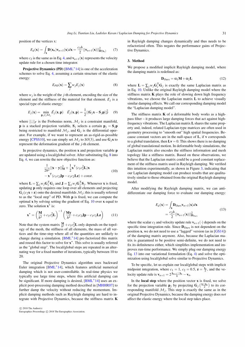
The stiffness matrix K of a deformable body works as a high-pass filter – it produces large damping forces that act against high-frequency vibrations. The Laplacian matrix L shares the same prop-erty and, indeed, related Laplacian-type matrices are often used ingeometry processing to "smooth out" high spatial frequencies. Be-cause constant vectors are in the null-space of L, if v correspondsto a global translation, then Lv= 0. This shows there is no dampingof global translational motion. In deformable body simulations, theLaplacian matrix also encodes the stiffness information and meshtopology like a stiffness matrix. Based on these observations, webelieve that the Laplacian matrix could be a good constant replace-ment of the stiffness matrix used in Rayleigh damping. We verifiedthis intuition experimentally, as shown in Figure 3, indicating thatour Laplacian damping model can produce results that are qualita-tively similar to those obtained from the original Rayleigh dampingmodel.

After modifying the Rayleigh damping matrix, we can anti-differentiate our damping force to evaluate our damping energy:

Ed(x) =∫

xDOursvn+1(x)dx

=c2h2||vn+1(x)||2DOurs

(13)

where the scalar c2 and velocity update rule vn+1(·) depends on thespecific time integration rule. Since DOurs is not dependent on theposition x, we do not need to use a “lagged” version (as in [GS14])of the damping matrix anymore. Also, because the Laplacian ma-trix is guaranteed to be positive semi-definite, we do not need tofix its definiteness either, which simplifies implementation and im-proves run-time performance. We simply plug our damping energyEq. 13 into our variational formulation (Eq. 4) and solve the opti-mization using local/global solve similar to Projective Dynamics.

To be specific, let us explain our local/global steps with implicitmidpoint integration, where c1 = 1, c2 = 0.5, z = xn

2 , and the ve-locity update rule is vn+1 = 2 xn+1−xn

h −vn.

In the local step where the position vector x is fixed, we solvefor the projection variable p j by projecting G j

( x+xn2)

to its cor-responding manifold M j. This step is exactly the same as in theoriginal Projective Dynamics, because the damping energy does notaffect the elastic energy where the local step takes place.


31


Example #Verts #Elems Integration Method Integration Time Integration Time Damping(without damping) (with damping) Overhead

ribbon (Figure 2) 549 728 implicit midpoint 10ms 10ms <1msbar (Figure 8) 738 1920 implicit midpoint 40ms 43ms 3mspenguin (Figure 1) 1979 6915 implicit midpoint 151ms 151ms <1msdummy (Figure 5) 4492 16890 implicit midpoint 670ms 674ms 4mspig (Figure 3) 5122 16505 implicit midpoint 477ms 486ms 9mshair (Figure 7) 1900 600 backward Euler 42ms 43ms 1ms

Table 1: Summary of our example simulations, all using the Projective Dynamics framework with 10 iterations. The “Integration Time” istotal time per frame of our method with / without damping.

In the global step where the projection variable p is already com-puted, we compute the optimal positions by solving the followingproblem:

12h2 ||x−y||2M +

12

xT(14

L)x−xT(12

Jp− 12

Lz)

+h4

∣∣∣∣∣∣2 x−xn

h−vn

∣∣∣∣∣∣2DOurs

+ const. (14)

which is exactly Eq. 10 with our damping energy Eq. 13 appendedat the end. The exact solution x∗ of this global problem can becomputed analytically as follows:

x∗ =(

Mh2 +

14

L+2h

DOurs

)−1

(Myh2 +

12

Jp− 12

Lz+DOurs(2h

xn +vn)

) (15)

Note that because DOurs is the combination of the mass matrix Mand the Laplacian matrix L, we can prefactorize the system ma-trix M

h2 +14 L+ 2

h DOurs as well. Therefore the global system can besolved efficiently at run time. As we can see from Table 1, the over-head of adding damping with our method is typically very smallbecause we do not disturb the efficient local/global solve processof Projective Dynamics.

4. Results

Table 1 summarizes all of our experiments including the run timesfor our method utilizing the Projective Dynamics framework. Allof our simulations use ten Projective Dynamics iterations. We cansee that our damping model adds only a very small computingoverhead compared to Projective Dynamics without damping. Thissmall computational cost is spent on evaluating DOurs(

2h xn +vn) in

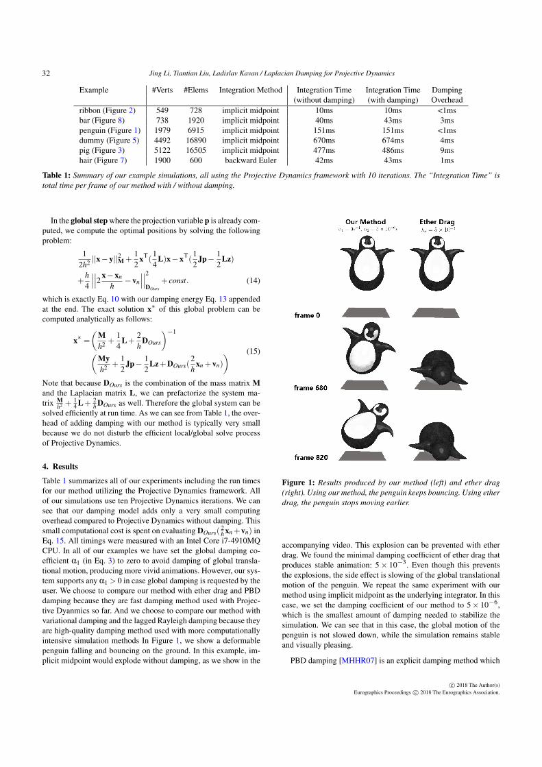
Eq. 15. All timings were measured with an Intel Core i7-4910MQCPU. In all of our examples we have set the global damping co-efficient α1 (in Eq. 3) to zero to avoid damping of global transla-tional motion, producing more vivid animations. However, our sys-tem supports any α1 > 0 in case global damping is requested by theuser. We choose to compare our method with ether drag and PBDdamping because they are fast damping method used with Projec-tive Dyanmics so far. And we choose to compare our method withvariational damping and the lagged Rayleigh damping because theyare high-quality damping method used with more computationallyintensive simulation methods In Figure 1, we show a deformablepenguin falling and bouncing on the ground. In this example, im-plicit midpoint would explode without damping, as we show in the

Figure 1: Results produced by our method (left) and ether drag(right). Using our method, the penguin keeps bouncing. Using etherdrag, the penguin stops moving earlier.

accompanying video. This explosion can be prevented with etherdrag. We found the minimal damping coefficient of ether drag thatproduces stable animation: 5× 10−3. Even though this preventsthe explosions, the side effect is slowing of the global translationalmotion of the penguin. We repeat the same experiment with ourmethod using implicit midpoint as the underlying integrator. In thiscase, we set the damping coefficient of our method to 5× 10−6,which is the smallest amount of damping needed to stabilize thesimulation. We can see that in this case, the global motion of thepenguin is not slowed down, while the simulation remains stableand visually pleasing.

PBD damping [MHHR07] is an explicit damping method which


32


Figure 2: Our method makes the ribbon coil in a natural and fabric-like fashion, similar to ribbon motions seen in rhythmic gymnasticsperformances. In contrast, PBD damping introduces unnatural early rotation of the tail of the ribbon, as if the ribbon was a rigid bar ratherthan fabric. The arrows point out the differences in the motion of the ribbon tail.

preserves both linear and angular momenta. However, since this isachieved by explicitly factoring out global rigid motion, the PBDdamping might preserve momenta in an unnatural, non-physicalway. In Figure 2, we show an example of this behavior using a sim-ulated ribbon attached to a wand. The wand circles around whiletranslating backwards, similar to a performance of rhythmic gym-nast. With the PBD damping applied to the ribbon, the tail of theribbon is moving when the end attached to the wand just startedrotating. But in real physical world, other than rigid body, the ve-locities cannot be transported immediately from one end to theother. The velocities from one end of the object are non-physicallytransported to velocities in the opposite end of the object, and theentire ribbon starts spinning almost like a rigid body. In contrast,our method models local damping forces, resulting in natural coil-ing motion of the ribbon as seen in real-world gymnastics perfor-mances.

In Figure 3, the snout of a pig is pulled and released, result-ing in a comical animation. We compared our method with laggedRayleigh damping [GS14], noticing the methods differ only insmall details such as the motion of the ears. The visual differ-ences are hard to distinguish without careful examination. Thelagged Rayleigh damping uses the definiteness-fixed Hessian ma-trix from the previous time step. Because this matrix changes ateach frame, we recompute the Cholesky factorization each frame,which is slower than our method, see Figure 4. However, we notethat faster numerical methods for the lagged Rayleight dampingare possible [GS14]. In Figure 5 we compare our method withthe “variational damping” approach introduced by Kharevych andcolleagues [KYT∗06]. We implemented variational damping in aseparate integration step, where the previous state is treated as rest-pose configuration. The resulting optimization problem is solvedby Newton’s method, which is more computationally intensive thanProjective Dynamics. The visual difference of the final result withour damping method and the variational damping is barely notice-able, but our method is much faster, as shown in Figure 6.

In Figure 7, we simulate hair strands as a mass-spring system,

shaken from side to side. In this simulation, we use backward Eu-ler and observe that its artificial numerical damping is not suffi-cient – the hair is too bouncy. With our method, we can introduceadditional damping and achieve a more sensible hair animation. InFigure 8 we show that our damping method behaves well under re-

Figure 3: Results produced by our method (left) and the laggedRayleigh damping [GS14] (right). Our method looks almost thesame as the lagged Rayleigh damping, but our method is muchfaster, as shown in Figure 4.


33


02468

101214

1 101 201 301 401 501 601 701 801 901 1001

�m

e (s

ec)

frame number

Timing for Each Frame

Our Method Lagged Rayleigh Damping

Implicit Midpoint without Damping

Figure 4: Computing time per animation frame for our method withimplicit midpoint, lagged Rayleigh damping, and implicit midpointwithout damping in the deformable pig animation (Figure 3). Allmethods use ten iterations.

Figure 5: Results produced by our method (left) and variationaldamping are visually similar, but our method is much faster, asshown in Figure 6.

finement. In this example, a thin sheet is fixed at one edge, and theother end drops freely under gravity. Notice that the results for timesteps of 1.65ms and 0.165ms are very similar, but are different fortime steps of 33ms.

5. Limitations and Future Work

Our method shares one limitations with Projective Dynamics: mod-ifications of the connectivity of the simulated system or its param-eters (including the damping coefficient) require re-factorizationof the Cholesky factors. Our method conserves linear momentum,but does not conserve angular momentum exactly. In the future,we believe that we can derive a modification of our method to ex-actly conserve angular momentum. Another avenue for future workwould involve extending our method to more advanced dampingmodels, such as Caughey damping or example-based damping de-sign [XB17].

6. Conclusion

We introduced a new implicit damping method which can be com-bined with various time integration schemes under the Projective

0

1

2

3

4

5

6

7

1 101 201 301 401 501 601 701 801 901 1001

�m

e(se

c)

frame number

Timing for Each Frame

Our Method Varia�onal Damping Implicit Midpoint without Damping

Figure 6: Computing time per animation frame for variationaldamping, implicit midpoint without damping, and implicit midpointwith our method. Times are for the dummy-punching simulationshown in Figure 5.

Figure 7: Hair animation with backward Euler with damping (ourmethod, left) and without damping (backward Euler only, right).

Dynamics framework. Our method produced higher quality resultsthan explicit damping methods. Unlike more expensive implicitdamping methods such as lagged Rayleigh damping and varia-tional damping, our method did not significantly reduce the per-formance of Projective Dynamics. The visual results of our methodwere comparable to results produced with more computationallyintensive implicit damping methods. We believe our new dampingmethod will find use in interactive applications such as games orsurgical training simulators.

Acknowledgements

We thank Junior Rojas, Saman Sepehri, and Cem Yuksel for manyinspiring discussions. We also thank Yasunari Ikeda for help withhair rendering, Nathan Marshak and Dimitar Dinev for proofread-ing, Shirley Han and Jessica Hair for narrating the accompanyingvideo. This work was supported by NSF awards IIS-1622360 andIIS-1350330


34


Figure 8: Convergence experiment with a flexible sheet simulatedwith different time steps. Small time steps lead to similar results.

References

[BMF05] BRIDSON R., MARINO S., FEDKIW R.: Simulation of clothingwith folds and wrinkles. In ACM SIGGRAPH 2005 Courses (2005),ACM, p. 3. 2

[BML∗14] BOUAZIZ S., MARTIN S., LIU T., KAVAN L., PAULY M.:Projective dynamics: fusing constraint projections for fast simulation.ACM Trans. Graph. 33, 4 (2014), 154. 1, 3

[CAP17] CHEN Y. J., ASCHER U., PAI D.: Exponential rosenbrock-euler integrators for elastodynamic simulation. IEEE Transactions onVisualization and Computer Graphics (2017). 1

[CO65] CAUGHEY T., O’KELLY M. E.: Classical normal modes indamped linear dynamic systems. Journal of Applied Mechanics 32, 3(1965), 583–588. 2

[CPSS10] CHAO I., PINKALL U., SANAN P., SCHRÖDER P.: A simplegeometric model for elastic deformations. In ACM SIGGRAPH 2010Papers (2010), SIGGRAPH ’10, ACM, pp. 38:1–38:6. 3

[FM17] FRÂNCU M., MOLDOVEANU F.: Unified simulation of rigid andflexible bodies using position based dynamics. 1

[GMD13] GLONDU L., MARCHAL M., DUMONT G.: Real-time sim-ulation of brittle fracture using modal analysis. IEEE Transactions onVisualization and Computer Graphics 19, 2 (2013), 201–209. 1

[GS14] GAST T. F., SCHROEDER C.: Optimization integrator for largetime steps. In Eurographics/ACM SIGGRAPH Symposium on ComputerAnimation (Copenhagen, Denmark, 2014), Eurographics Association. 2,3, 5

[KYT∗06] KHAREVYCH L., YANG W., TONG Y., KANSO E., MARS-DEN J. E., SCHRÖDER P., DESBRUN M.: Geometric, variational inte-grators for computer animation. In Proceedings of the 2006 ACM SIG-GRAPH/Eurographics symposium on Computer animation (2006), Eu-rographics Association, pp. 43–51. 2, 5

[LBK17] LIU T., BOUAZIZ S., KAVAN L.: Quasi-newton methods forreal-time simulation of hyperelastic materials. ACM Transactions onGraphics (TOG) 36, 3 (2017), 23. 1, 2

[LBOK13] LIU T., BARGTEIL A. W., O’BRIEN J. F., KAVAN L.: Fastsimulation of mass-spring systems. ACM Transactions on Graphics 32,6 (Nov. 2013), 209:1–7. (Proceedings of ACM SIGGRAPH Asia 2013,Hong Kong). 1

[LKSH08] LLOYD B. A., KIRAC S., SZÉKELY G., HARDERS M.: Iden-tification of dynamic mass spring parameters for deformable body sim-ulation. In Eurographics (Short Papers) (2008), Citeseer, pp. 131–134.1

[MHHR07] MÜLLER M., HEIDELBERGER B., HENNIX M., RATCLIFFJ.: Position based dynamics. Journal of Visual Communication andImage Representation 18, 2 (2007), 109–118. 1, 2, 3, 4

[MTGG11] MARTIN S., THOMASZEWSKI B., GRINSPUN E., GROSSM.: Example-based elastic materials. In ACM Transactions on Graphics(TOG) (2011), vol. 30, ACM, p. 72. 2

[Ray96] RAYLEIGH J. W. S. B.: The theory of sound. Macmillan 2(1896). 2

[SSF13] SU J., SHETH R., FEDKIW R.: Energy conservation for thesimulation of deformable bodies. IEEE Transactions on Visualizationand Computer Graphics 19, 2 (Feb. 2013), 189–200. 1, 2

[Tau95] TAUBIN G.: A signal processing approach to fair surface design.In Proceedings of the 22nd annual conference on Computer graphicsand interactive techniques (1995), ACM, pp. 351–358. 1

[TPBF87] TERZOPOULOS D., PLATT J., BARR A., FLEISCHER K.:Elastically deformable models. SIGGRAPH Comput. Graph. 21, 4 (Aug.1987), 205–214. 2

[Wil02] WILSON E. L.: Three-Dimensional Static and Dynamic Analysisof Structures, 3rd ed. Computers and Structures, Inc., 2002. 1

[XB17] XU H., BARBIC J.: Example-based damping design. ACMTrans. Graph. 36, 4 (July 2017), 53:1–53:14. 2, 6

[Zha04] ZHANG H.: Discrete combinatorial laplacian operators for dig-ital geometry processing. In Proceedings of SIAM Conference on Ge-ometric Design and Computing. Nashboro Press (2004), pp. 575–592.1

Appendices

A. Assembly of G j and p

A.1. Finite Element MethodWe denote the number of vertices as n and the number of elements(tetrahedra) as m. For one single tetrahedron, the four vertex indicesare i1, i2, i3, i4. In this tetrahedron, we assume that i2 < i1 < i3 < i4

G j = D−TM A j⊗ I3 (16)

where DM is the reference shape matrix, and A j ∈ R3×n can bewritten as

A j =

( i2 i1 i3 i41 −1

1 −11 −1

)(17)

where i1, i2, i3, i4 denote the column numbers, and all the entriesother than 1 and -1 are 0.

p =

p1p2...

pm

(18)

where p j ∈ R9×1, p ∈ R9m×1.

A.2. Spring

We denote the number of vertices as n and the number of ele-ments(springs) as m. For one single spring, the two vertex indicesare i1 and i2.

G j =1r

A j⊗ I3 (19)


35


where r is the rest length of the spring, and A j ∈ R1×n can bewritten as

A j = (i1 i21 −1 ) (20)

where i1, i2 denote the column numbers, and all the entries otherthan 1 and -1 are 0.

p =

p1p2...

pm

(21)

where p j ∈ R3×1, p ∈ R3m×1.

B. Proof of preservation of linear momentumFor a single tetrahedron, the vertices of which are x1, x2, x3, x4,the velocities of each vertex are v1, v2, v3, v4. We consider thecase where the motion of the tetrahedron is pure translation, whichmeans v1 = v2 = v3 = v4.

The deformation gradient is given as

F = DSD−1M (22)

We vectorize DS as

vec(DS) =

[x1−x4x2−x4x3−x4

]= (Aj⊗ I3)x

(23)

Thus the deformation gradient can be vectorized as well as:

vec(F) = vec(DSD−1M )

= (D−TM ⊗ I3)vec(DS)

= (D−TM ⊗ I3)(A j⊗ I3)x

= (D−TM A j⊗ I3︸︷︷︸G j∈R9×3n

)x

(24)

Our corresponding Laplacian matrix will be:

L = ∑ω j(D−TM A j⊗ I3)

T (D−TM A j⊗ I3)

= ∑ω j(D−TM A j)

T ⊗ I3D−TM A j⊗ I3

= ∑ω jAjT D−1

M D−TM A j⊗ I3

(25)

yielding the damping force:

Lv = ∑ω jATj D−1

M D−TM (A j⊗ I3v) (26)

where

A j⊗ I3v =

(v1−v4v2−v4v3−v4

)= 0 (27)

Therefore, the damping force Lv is 0 under the translation mode,preserving the linear momentum of the system.


36

laplacian damping for projective dynamics

Documents