computational methods for modelling and analysing ... · computational methods for modelling and...

Tampere University of Technology

Computational Methods for Modelling and Analysing Biological Networks

CitationLarjo, A. (2015). Computational Methods for Modelling and Analysing Biological Networks. (Tampere Universityof Technology. Publication; Vol. 1289). Tampere University of Technology.

Year2015

VersionPublisher's PDF (version of record)

Link to publicationTUTCRIS Portal (http://www.tut.fi/tutcris)

Take down policyIf you believe that this document breaches copyright, please contact [email protected], and we will remove access tothe work immediately and investigate your claim.

Download date:16.07.2018

https://tutcris.tut.fi/portal/en/publications/computational-methods-for-modelling-and-analysing-biological-networks(24628d0e-fce7-484d-93a9-83e2bdff8575).html

Tampereen teknillinen yliopisto. Julkaisu 1289 Tampere University of Technology. Publication 1289 Antti Larjo Computational Methods for Modelling and Analysing Biological Networks Thesis for the degree of Doctor of Science in Technology to be presented with due permission for public examination and criticism in Sähkötalo Building, Auditorium S2, at Tampere University of Technology, on the 27th of March 2015, at 12 noon. Tampereen teknillinen yliopisto - Tampere University of Technology Tampere 2015

ISBN 978-952-15-3483-6 (printed) ISBN 978-952-15-3490-4 (PDF) ISSN 1459-2045

ReviewersDr. Tero AittokallioDr. Florence d’Alché-Buc

OpponentDr. Jens Lagergren

Abstract

The main theme of this thesis is modelling and analysis of biological networks.Measurement data from biological systems is being produced at such a pace thatit is impossible to make use of it without computational models and inferencealgorithms. The methods and models presented here aim at allowing to extractrelevant relationships from the masses of data and formulating complex biologicalhypotheses that can be studied via simulation.

The problem of learning the structure of a popular method class, Bayesiannetworks, from measurement data is investigated in this thesis, and an improve-ment to the standard method is presented that facilitates finding the correctnetwork structure. Furthermore, this thesis studies active learning, where thestructure inference algorithm can itself suggest measurements to be made. Activelearning is applied to realistic scenarios with measured datasets and an activelearning method that can deal with heterogeneous data types is presented.

Another focus of this thesis is on analysing networks whose structure isknown. The utility of a standard method for selecting beneficial mutations inmetabolic networks is evaluated in the context of engineering the network toproduce a desired substance at a higher rate than normally. Metabolic networkmodelling is also used in conjunction with a simulation of a biochemical networkcontrolling bacterial movement in a state-based and executable framework thatcan integrate different submodels. This combined model is then used to simulatethe behaviour of a population of bacteria.

In summary, this thesis presents improvements on methods for learning net-work structures, evaluates the utility of an analysis method for identifying suit-able mutations for producing a substance of interest, and introduces a state-based modelling framework capable of integrating several submodels.

iii

Preface

This thesis is the result of work done mainly at the Department of Signal Pro-cessing, Tampere University of Technology, and also partly when working atDepartment of Information and Computer Science at Aalto University Schoolof Science, and during a short stay at Microsoft Research, Cambridge, UK. Fi-nancial support from Academy of Finland’s Centre of Excellence in MolecularSystems Immunology and Physiology Research (SyMMyS), Emil Aaltonen Foun-dation, TISE graduate school, the Finnish Cultural Foundation, and Tuula andYrjö Neuvo Foundation is gratefully acknowledged.

I acknowledge gratefully my indebtedness to Prof. Olli Yli-Harja for providingthe possibility of working on this subject and supervising this thesis. I also recordmy deep appreciation to my other thesis supervisor, Prof. Harri Lähdesmäki, forhis insightful comments and being a hard-working and inspiring example. Themembers of the Computational Systems Biology research group are also acknowl-edged for creating a great, albeit occasionally distracting atmosphere. A specialmention for making it more fun to go to work goes to former cellmates TimoErkkilä, Pekka Ruusuvuori, Jenni Seppälä and Tarmo Äijö. Also, extra credit isdue to Antti Ylipää, Matti Nykter and Virpi Kivinen, for numerous lunch andcoffee breaks. I am also grateful to Tommi Aho, Ville Santala, Prof. Matti Karpand Dr. Hillel Kugler for collaboration.

I also want to thank the secretaries of the department, and in particularVirve Larmila, without whom the department would undoubtedly not exist.

Above all, I express my sincerest gratitude to my wonderful family and myparents and brother.

v

List of Abbreviations

ABCP algorithm for blocking competing pathwaysBN Bayesian networkCW clockwiseCCW counter-clockwiseDNA deoxyribonucleic acidEM elementary modeEP extreme pathwayFBA flux balance analysisGEM genome-scale modelGRN gene regulatory networkMFA metabolic flux analysisMCMC Markov chain Monte CarlomRNA mature RNAnt nucleotideODE ordinary differential equationqPCR quantitative real-time PCRRNA ribonucleic acidSNP single-nucleotide polymorphismUML Unified Modeling Language

vii

Contents

Abstract iii

Preface v

List of Abbreviations vii

Contents ix

List of Included Publications xi

1 Introduction 11.1 Objectives of the thesis . . . . . . . . . . . . . . . . . . . . . . . . 31.2 Outline of the thesis . . . . . . . . . . . . . . . . . . . . . . . . . 4

2 Models of biological networks 52.1 Gene regulatory networks and signalling networks . . . . . . . . . 52.2 Metabolic networks . . . . . . . . . . . . . . . . . . . . . . . . . . 62.3 Biochemical reaction networks . . . . . . . . . . . . . . . . . . . . 7

2.3.1 Bacterial chemotaxis . . . . . . . . . . . . . . . . . . . . . 82.4 Executable models . . . . . . . . . . . . . . . . . . . . . . . . . . 102.5 Measurement techniques . . . . . . . . . . . . . . . . . . . . . . . 12

3 Bayesian networks 173.1 Definition of BNs . . . . . . . . . . . . . . . . . . . . . . . . . . . 183.2 Learning the structure of BNs . . . . . . . . . . . . . . . . . . . . 203.3 Markov Chain Monte Carlo . . . . . . . . . . . . . . . . . . . . . 22

3.3.1 Convergence . . . . . . . . . . . . . . . . . . . . . . . . . . 243.3.2 Proposal distribution . . . . . . . . . . . . . . . . . . . . . 25

3.4 Active learning . . . . . . . . . . . . . . . . . . . . . . . . . . . . 26

4 Modeling metabolic networks 314.1 Constraint-based models . . . . . . . . . . . . . . . . . . . . . . . 33

4.1.1 Flux balance analysis . . . . . . . . . . . . . . . . . . . . . 37

ix

x CONTENTS

5 Summary of the results 41

6 Conclusions 45

Publications 63

List of Included Publications

This thesis is a compound thesis consisting of the following 5 publications

I A. Larjo and H. Lähdesmäki, “Using multi-step proposal distributionfor improved MCMC convergence in Bayesian network structure learning,”submitted to EURASIP Journal on Bioinformatics and Systems Biology,2014.

II A. Larjo, H. Lähdesmäki, M. Facciotti, N. Baliga, I. Shmulevich,and O. Yli-Harja, “Active learning of Bayesian network structure in a re-alistic setting,” in Fifth International Workshop on Computational SystemsBiology (WCSB 2008), Leipzig, Germany, June 11-13, 2008, pp. 85-88.

III A. Larjo and H. Lähdesmäki, “Active learning for Bayesian networkmodels of biological networks using structure priors,” in IEEE Interna-tional Workshop on Genomic Signal Processing and Statistics, Houston,TX, USA, November 17-19, 2013, pp. 78-81.

IV J.J. Seppälä*, A. Larjo*, T. Aho, O. Yli-Harja, M.T. Karp,and V. Santala, “Prospecting hydrogen production of Escherichia coliby metabolic network modeling,” International Journal of Hydrogen En-ergy, vol. 38, no. 27, pp. 11780-11789, 2013.

V H. Kugler*, A. Larjo*, and D. Harel, “Biocharts: A visual formalismfor complex biological systems,” Journal of the Royal Society Interface,vol. 7, no. 48, pp. 1015–1024, 2010.

* denotes equal contribution.

Author’s Contributions to the Publications

The author of this thesis contributed to the included publications as follows:In Publications I and III the author designed and implemented the methods,

derived the mathematical proofs, ran simulations, and wrote the manuscript. InPublication II the author implemented the methods, did all the simulations andwrote the manuscript.

xi

xii CONTENTS

In Publication IV the author performed all metabolic simulations except forthe ABCP method, and wrote the corresponding sections of the manuscript.This publication has also been part of the thesis of J. Seppälä, who did thebiological work for the manuscript.

In publication V the author designed and implemented the model systemand did all the modeling, simulation and analysis work. H. Kugler supervisedthe study. The manuscript was written by A. Larjo and H. Kugler.

Chapter 1

Introduction

Models have an essential role in may fields of science (and not least in biology(Mogilner et al., 2006)). They aim at representing the system being studied asaccurately as possible and represent crystallizations of the knowledge gained bystudying the system. Models themselves can be studied and simulated, allowing,e.g., quantitative testing of hypotheses, producing predictions, and interpretingmeasurement data.

As an example, a scientist may have a hypothesis about a complex systemand if the hypothesis can be formalized as a model, then comparing the sim-ulation results to new measurements either lends support to the hypothesis orsuggests something needs to be fixed. This validation of hypotheses can becomeimpossible to perform without the help of computational models and simula-tions that can be run on computers. The reason is the growing complexity ofthe hypotheses, which is happening in many fields of science thanks to increas-ing capability to measure more variables at the same time with greater accuracy.This is one of the reasons computational modelling has lately become a centralpart of research in many fields.

Another task impossible to perform “manually” or “by eye” is finding patternsor structure in big datasets that would allow gaining knowledge for exampleabout which entities function together and what are their causal relationships.By using machine learning and suitable computational models as well as analysisand simulation methods, even huge datasets consisting of heterogeneous datatypes can be sifted through and meaningful relationships extracted.

Biology has traditionally been a hypothesis-driven science but it can be ar-gued that lately it has become more and more data-driven because of the recentwhole-cell or genome-wide measurements, together with machine learning ap-proaches. It has also been argued that, largely due to improved computationaland measurement techniques, there has been a paradigm shift form the tradi-tional reductionism towards a holistic approach called systems biology.

In the last decades, network models have become extremely popular (Barabasi,

1

2 CHAPTER 1. INTRODUCTION

2002; Barabasi and Oltvai, 2004). This growth in interest is because people arestudying larger systems of interacting entities that are naturally modelled asnetworks, and to a large extent the network models and their development iswhat has in fact allowed studying such systems. At least one enabling reason isthe ability brought with increased computing power to learn and analyse largermodels. Networks can be found in almost every aspect of life and they havebeen extensively studied using methods from physics, control theory, and graphtheory, becoming something dubbed “network science" (Lewis, 2011). Plenty ofattention has been paid to the topological properties of networks, such as degreedistributions, network motifs and modules (Zhu et al., 2007).

Identifying the network structure of an underlying system from measurementdata is of great interest in many areas. This process is called inference, structurelearning or reverse-engineering of the networks. In this thesis, the inferenceproblem is studied in the field of biological sciences where data suitable for thispurpose is nowadays ample. It can actually be argued that the huge progress ingenerating measurement data has not been completely followed by developmentof computational analysis and modelling methodologies in biosciences. Yet, thereis a pressing need to understand how cellular networks are built and how theyfunction as they govern the cellular activities, and problems in their ability tofunction properly can cause for example trouble for immune system and elicitdiseases such as cancer.

The model class used in this thesis for inference of network structure isBayesian networks and they are based on two sets of methods that have be-come very popular lately. Bayesian networks are a model class with roots inBayesian methods and statistics (Pearl, 1985; Eddy, 2004; Beaumont and Ran-nala, 2004). Bayesian methods are increasingly popular, some seeing them evenas a new paradigm for statistics. Inarguably, they are often able to solve trickyproblems, but they do bring about conceptual and even philosophical issues thatare somewhat debated (Lindley, 2000).

The other set of methods that has in the last decades become popular isMarkov chain Monte Carlo (MCMC), which is a class of estimation methodsthat rely on heavy sampling and can in practice be only done with computers(Diaconis, 2009). In fact, MCMC methods (and in general Monte Carlo methods)have been able to overcome many computational problems in Bayesian methods,together with increasing computing capability. Consequently, the big increase ininterest in Bayesian methods since the 1980s was likely mainly due to discoveryof Markov Chain Monte Carlo methods.

For networks whose structure is known, it is of interest to analyse and simu-late them, e.g., to examine behaviour that can arise due to different conditionsand to predict changes in phenotypes resulting from modifications to the networkstructure. An example of a model class where such analysis is routinely doneis metabolic networks, whose structure can be for some organisms (especially

1.1. OBJECTIVES OF THE THESIS 3

bacteria) well known. Metabolic networks are also studied in this thesis.

1.1 Objectives of the thesis

The objective of the thesis is to present computational methods for inference ofnetwork structures and to simulate biological networks for which the structureis already known.

Although Bayesian networks are a theoretically sound and justified methodfor modelling gene regulatory networks, as well as protein-protein interactionnetworks, inferring the Bayesian network structure from experimental data canbe challenging. For all but the smallest networks one must resort to Markovchain Monte Carlo methods but a major problem with them is difficulty inconvergence. To alleviate this problem, Publication I investigates a new wayto propose transitions in the MCMC chain that is shown to increase rate ofconvergence by escaping local maxima.

Another problem inherent in the inference of network structure is how tomake sure that the learnt relationships are causal and not mere non-causal re-lationships (like correlations). Causality can be separated from correlation byintroducing interventions but they can be costly to perform and selecting themin non-optimal way might waste resources. Thus, selecting interventions in themost beneficial way is an important problem and methods called active learningtry to perform this. Publication II looks at the performance of one such methodin structure inference of Bayesian networks while Publication III studies how tocombine more than one data type in active learning.

Metabolic engineering is a field of growing importance as there is an in-creasing need to modify and design biological organisms to produce beneficialsubstances and get rid of harmful ones. Traditional methods for this rely onbiological experiments and more or less luck. Model-based selection of modifica-tions has the potential to make the process much faster and at least considerablynarrow down the choices that need to be tested. Publication IV looks at thisproblem in the context of trying to find knock-out mutations for increased hy-drogen production.

Publication V investigates the integration of more than one model, whichis important as the submodels by themselves are not always able to explainthe observed behaviour. Another aspect is the utilization of executable models,which is done using a framework where modelled systems are described withstates and transitions between them. The lower-level functionality is encodedusing a programming language so that the whole model is directly compilable toa computer executable program.

4 CHAPTER 1. INTRODUCTION

1.2 Outline of the thesis

Chapter 2 describes how modelling of certain biological networks can be done.It also introduces chemotaxis as an example system and briefly describes thestochastic simulator and chemotactic model used in Publication V.

Chapter 3 presents the theory needed in Bayesian network structure learning,including definition of Bayesian networks and Markov chain Monte Carlo meth-ods, which are the necessary basis for Publication I. Active learning in contextof Bayesian networks is also shortly presented in Chapter 3 as this is the subjectof Publications II and III.

In Chapter 4, methods for analysing metabolic networks under steady-stateare presented. These so called constraint-based methods include flux balanceanalysis, which is applied in Publications IV and V.

Chapter 5 summarizes the results of Publications I-V. Finally, Chapter 6contains concluding remarks with some possible future directions, and the in-cluded publications follow after the list of references.

Chapter 2

Models of biological networks

Development of a biological system and its responses to stimuli depend on acomplex interplay between hundreds or thousands of molecules and these actionsneed to take place in a coordinated and robust manner while ensuring that oftensubtle signals from environment are taken into account. Due to the interactorynature, biological systems are commonly described as networks where nodesrepresent the entities and edges the interactions between them. The emergence ofhigh-throughput measurement technologies has enabled identification of networkcomponents and their interactions in large-scale and spurred the development ofinference and modelling methods.

Although entities of a certain type do not work in isolation, one is usuallyrestricted to concentrate on only some subsystems because of for example limitedmeasurement data and modelling difficulties. Networks of these subsystem typesinclude, e.g., transcription factor binding, protein-protein interaction, proteinphosphorylation, metabolic interaction and genetic interaction networks (Zhuet al., 2007). Due to the diverse nature of molecules and interactions in thesedifferent subsystems, the models used to describe these systems and methods toanalyse and simulate them are often different. This chapter shortly reviews thenetwork types and methods used to model the subsystems that are encounteredin the publications that are part of this thesis.

2.1 Gene regulatory networks and signalling networks

The states of genes can influence other genes, creating networks and cascades.The interaction is (always) indirect, mediated via the downstream products ofa gene. These can be for example RNA molecules or proteins that can bindthe DNA sequence controlling the expression of another gene (or also its ownin autoregulation) or for example inhibit the mRNA produced by another gene.Therefore, genes are meta-level entities in gene regulatory network (GRN) mod-elling and the levels of their expression results (mRNA molecules) are modelled

5

6 CHAPTER 2. MODELS OF BIOLOGICAL NETWORKS

instead. Transcription factor-binding networks are one type of gene regulatorynetworks, where mediation of a gene state is done via its produced protein thatbinds the DNA regions controlling expressions of other genes.

Recent developments of measurement techniques allow huge genomic datasetsto be produced. Some of the notable advancements relevant for inference of generegulatory networks include high-throughput gene expression measurements ca-pable of measuring the expression states of basically all genes at a time, whichcan be done using, e.g., cDNA microarrays (Schena et al., 1995) or RNA-seq(Mortazavi et al., 2008). Technologies to investigate which genes are being af-fected by a protein of interest include chromatin immunoprecipitation (ChIP)followed by either microarray measurement (ChIP-chip) (Ren et al., 2000) orDNA sequencing (ChIP-seq) (Johnson et al., 2007), both of which measure thegenomic binding sites of a protein.

Modelling GRNs has been under intense research and several different mod-els and methods to infer them from experimental data have been developed andused (Bansal et al., 2007; Karlebach and Shamir, 2008; Noor et al., 2013). Dif-ferent models include Boolean networks (Kauffman, 1969), probabilistic Booleannetworks (Shmulevich et al., 2002), Bayesian networks (Friedman et al., 2000),dynamic Bayesian networks (Ghahramani, 1998; Murphy and Mian, 1999), state-space models (Wu et al., 2004; Quach et al., 2007), rule-based simulations (Mey-ers and Friedland, 1984), information theoretic methods (Margolin et al., 2006;Zhao et al., 2006), ordinary and partial differential equations (De Jong, 2002),and Gaussian processes (Äijö and Lähdesmäki, 2009).

Cellular information processing and responses to environmental stimuli areoften implemented in the cells via signalling networks, which consist of inter-acting signalling molecules. These are usually proteins and their interactionscan cause changes in the states of phosphorylation, conformations, and physicallocations of the molecules. Measuring signalling protein expression as well asmodification state levels can also be done in a high-throughput fashion using forexample multi-color flow cytometry, and many of the methods used for GRNinference and modelling can and have been used also in context of signallingnetworks (Sachs et al., 2005).

In this thesis (Publications I, II and III) Bayesian networks are used for thepurpose of modelling biological networks, even though they are applicable tomuch wider set of problems than just biological ones. Bayesian networks aredealt with in Chapter 3.

2.2 Metabolic networks

Metabolism of a cell is the totality of processes responsible for convertingmolecules (called metabolites) into another molecules and producing energy andmaterial for growth and sustenance. Metabolism consists of a set of reactions

2.3. BIOCHEMICAL REACTION NETWORKS 7

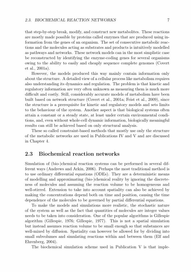
that step-by-step break, modify, and construct new metabolites. These reactionsare mostly made possible by proteins called enzymes that are produced using in-formation from the genes of an organism. The set of consecutive metabolic reac-tions and the molecules acting as substrates and products is intuitively modelledas pathways and networks. These network models can in the most simplistic casebe reconstructed by identifying the enzyme-coding genes for several organismsowing to the ability to easily and cheaply sequence complete genomes (Covertet al., 2001a).

However, the models produced this way mainly contain information onlyabout the structure. A detailed view of a cellular process like metabolism requiresalso understanding its dynamics and regulation. The problem is that kinetic andregulatory information are very often unknown as measuring them is much moredifficult and costly. Still, considerably accurate models of metabolism have beenbuilt based on network structure (Covert et al., 2001a; Feist et al., 2009), sincethe structure is a prerequisite for kinetic and regulatory models and sets limitsto the behaviour of the system. Another aspect is that biological systems oftenattain a constant or a steady state, at least under certain environmental condi-tions, and, even without whole-cell dynamic information, biologically meaningfulresults can still be achieved based on only structural analysis.

These so called constraint-based methods that mostly use only the structureof the metabolic networks are used in Publications IV and V and are discussedin Chapter 4.

2.3 Biochemical reaction networks

Simulation of (bio-)chemical reaction systems can be performed in several dif-ferent ways (Andrews and Arkin, 2006). Perhaps the most traditional method isto use ordinary differential equations (ODEs). They are a deterministic meansof modelling and approximating (bio-)chemical reality by ignoring the discrete-ness of molecules and assuming the reaction volume to be homogeneous andwell-stirred. Extension to take into account spatiality can also be achieved bymaking the concentrations depend both on time and position, causing the timedependence of the molecules to be governed by partial differential equations.

To make the models and simulations more realistic, the stochastic natureof the system as well as the fact that quantities of molecules are integer valuesneeds to be taken into consideration. One of the popular algorithms is Gillespiealgorithm (Gillespie, 1976; Gillespie, 1977). This is not a spatial simulationbut instead assumes reaction volume to be small enough so that substances arewell-mixed by diffusion. Spatiality can however be allowed for by dividing intosmall subvolumes and simulating reactions within and between them (Elf andEhrenberg, 2004).

The biochemical simulation scheme used in Publication V is that imple-


mented in the program StochSim (Morton-Firth and Bray, 1998; Le Novere andShimizu, 2001), which is a mesoscopic-scale stochastic simulator, whose intra-cellular simulations are non-spatial, assuming fast enough diffusion of substanceswithin a cell. The basic functioning of StochSim is such that first the length oftime-slice is chosen by the most rapid reaction and then, within each time slice,two objects (molecules) are chosen randomly and whether a reaction betweenthem happens is determined by a look-up table that tells the probabilities ofreactions happening. The main advantage of the algorithm is its capability ofhandling multi-state molecules, such as a receptor with different methylation orphosphorylation states that can affect the way it functions, which in Gillespiesimulation would require multiple (pseudo-)molecules. StochSim is also able tomodel changes taking place much faster than chemical reactions, such as lig-and binding or conformational changes, by changing such “fast flagged” statesaccording to a probability (that can depend for example on concentrations ofother substances) and only after that continue with the selected two species.

Many other simulation systems exist, including Smoldyn (Andrews and Bray,2004; Andrews, 2012), VCell (Loew and Schaff, 2001; Slepchenko and Loew,2010), Moleculizer (Lok and Brent, 2005), and AgentCell (Emonet et al., 2005).Of these at least the last one has been used to model E. coli chemotaxis that isalso the system modelled in Publication V.

2.3.1 Bacterial chemotaxis

The movement of a bacterium to a beneficial direction is made possible by itsability to sense gradients in its environment. There are several different stim-uli that can affect the movement, for example light (phototaxis) or tempera-ture (thermotaxis). Movement guided by chemical stimulus is called chemotaxis(Wadhams and Armitage, 2004; Armitage, 1999) and its direction can be eithertowards a higher concentration of a substance (positive chemotaxis) or awayfrom it (negative chemotaxis). The sensing is done in a temporal fashion duringmovement since the diameter of most bacteria are likely too small for sensinggradients across their diameter (Adler, 1975), though not necessarily in all cases(Thar and Kühl, 2003). Bacterial chemotaxis is being studied since it plays animportant part for example in pathogenicity and formation of biofilms. Bacterialchemotaxis also serves as an important and well-characterized model system.

Movement of many swimming bacteria consist of repeated straight runs fol-lowed by rapid changes (called tumbling) to another direction. The frequency oftumbling is controlled by the chemosensory system so that the more favourablethe conditions for the bacteria are, the more infrequent the tumbling.

The best-studied case of chemotaxis is the movement of Escherichia coli bac-teria (Adler, 1966; Berg and Brown, 1972) and is also used as a model system inPublication V. The helical semi-rigid filaments (called flagella) or the bacteriumare each rotated by its own motor, in either clockwise (CW) or counter-clockwise

2.3. BIOCHEMICAL REACTION NETWORKS 9

Tar$

CheW$ CheA$p

CheY$

CheY$p

motor$

CheZ$

CheB$

CheB$

p

-CH3 CheR$+CH3

Asp$

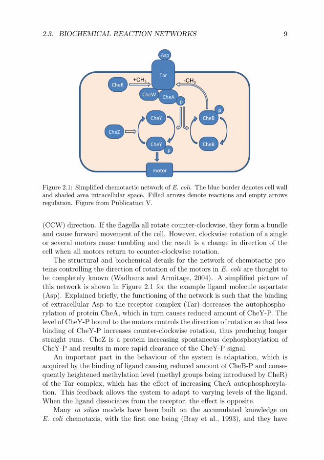
Figure 2.1: Simplified chemotactic network of E. coli. The blue border denotes cell walland shaded area intracellular space. Filled arrows denote reactions and empty arrowsregulation. Figure from Publication V.

(CCW) direction. If the flagella all rotate counter-clockwise, they form a bundleand cause forward movement of the cell. However, clockwise rotation of a singleor several motors cause tumbling and the result is a change in direction of thecell when all motors return to counter-clockwise rotation.

The structural and biochemical details for the network of chemotactic pro-teins controlling the direction of rotation of the motors in E. coli are thought tobe completely known (Wadhams and Armitage, 2004). A simplified picture ofthis network is shown in Figure 2.1 for the example ligand molecule aspartate(Asp). Explained briefly, the functioning of the network is such that the bindingof extracellular Asp to the receptor complex (Tar) decreases the autophospho-rylation of protein CheA, which in turn causes reduced amount of CheY-P. Thelevel of CheY-P bound to the motors controls the direction of rotation so that lessbinding of CheY-P increases counter-clockwise rotation, thus producing longerstraight runs. CheZ is a protein increasing spontaneous dephosphorylation ofCheY-P and results in more rapid clearance of the CheY-P signal.

An important part in the behaviour of the system is adaptation, which isacquired by the binding of ligand causing reduced amount of CheB-P and conse-quently heightened methylation level (methyl groups being introduced by CheR)of the Tar complex, which has the effect of increasing CheA autophosphoryla-tion. This feedback allows the system to adapt to varying levels of the ligand.When the ligand dissociates from the receptor, the effect is opposite.

Many in silico models have been built on the accumulated knowledge onE. coli chemotaxis, with the first one being (Bray et al., 1993), and they have


been observed to capture the main chemotactic behaviour very well. Thus, choos-ing such a very well developed model (implemented and presented in Morton-Firth et al. (1999)) as a part of our model in Publication V allows us to concen-trate on other issues of the modelling and may also hint that if the results donot conform with experiments then the problem is most probably in the otherparts of our model. Comprehensive reviews on modelling bacterial chemotaxisinclude (Tindall et al., 2008b) and (Tindall et al., 2008a).

Chemotactic assays

The most used chemotactic assays include capillary assay tubes (Adler, 1966)and swarm plates. Capillary assay tube is a cylinder filled with a nutritiousmedium and the other end of the tube is placed into a medium containing apopulation of bacteria. If the tube contains a nutrient favoured by the bacteria,they start moving into the tube, all the while consuming the nutrient substrateand thus creating a concentration gradient towards the other end of the tube.This gradient moves with the bacteria and the resulting population behaviouris a band of bacteria travelling along the tube. Depending on the medium andbacteria, more than one bands can be formed.

In swarm plates a population of bacteria is positioned to a small area on aplate containing a medium with chemoattractant(s). Population behaviour sim-ilar to tube assays is observed as expanding concentric rings, resulting from thesame phenomenon of self-created concentration gradients. Also more complexbehaviour is observed for many bacteria, such as formation of patterns. Theseare supposedly created by chemoattractants excreted and sensed by the cellsmoving themselves.

These phenomena derive from interplay between chemotaxis and metabolismin that the metabolic activity causes gradients of chemoattractants to form andthus creates an excitation of the chemotactic network. On the other hand,chemotactic behaviour drives the organism to environments with varying sub-strate profiles, thus having an effect on metabolic behaviour. This “communica-tion” between the metabolic and chemotactic networks was one of the aspectsmodelled in Publication V.

2.4 Executable models

Biochemical pathways presented in many textbooks and publications are rathereasy to comprehend but this is thanks to them covering a very limited scope(often in a simplified way). One feature of such models that can be considereda major shortcoming is that the exact meanings of symbols can vary from onepresentation to another. When trying to depict larger and more complex sys-tems or processes with numerous interconnections and (auto)regulatory loops, it

2.4. EXECUTABLE MODELS 11

quickly becomes impossible to understand how the system behaves without thehelp of computer simulations.

These facts clearly call for a modelling formalism defining unambiguousmeanings for the model entities and interactions, and also allows the system de-piction to be read by a computer and simulated. Additional advantage of such aformalism is that the models described using it are exchangeable and thus easilyshared between people studying the same system. The formal depiction shouldalso be such that it is easily converted between a view that is comprehensibleand easy to modify for humans and a format readable by computers.

Ways to formalize the notation of biological networks have been presented,for example process diagrams (Kitano et al., 2005) and molecular interactionmaps (Kohn et al., 2006), which are included (with some modifications) as sub-languages in the community-developed standard visual language called SystemsBiology Graphical Notation (SBGN) (Le Novere et al., 2009). These enablesharing of models using for example BioPAX (Demir et al., 2010) but usuallylack the information about how to simulate the model, which is often essentialin order to understand the dynamic processes.

Systems Biology Markup Language (SBML) (Hucka et al., 2003) and CellML(Lloyd et al., 2004) are also widely used as a means of exchanging and definingmodels and can incorporate information needed for the simulation of the model,for example as differential equation formulas of reaction rates. In models de-scribed using e.g. SBML, the simulation software is not predetermined but theuser is free to select any simulator that can read in SBML models. In some sensenot being restricted to a single simulator or algorithm is an advantage, but oneproblem with this scenario is that simulation results are not guaranteed to beexactly equivalent when the same model is simulated with two different simu-lators. Discrepancies can be for example due to different ODE solvers and/orparameters, all of which may not be explicitly stated in the model description.

A distinction can be made between computational and mathematical models(Fisher and Henzinger, 2007), the latter of which are the kind of “normal” mod-els consisting of, e.g., ODEs and requiring an algorithm for simulating them.Computational models are built from entities (called state machines (Fisher andHenzinger, 2007) that can also be small computer programs) having differentstates and the state changes are dependent on defined events, such as interac-tions with other entities. Composition of such entities constitutes a reactivesystem, the mathematical analysis of which can be impossible. However, themodel determines the sequence of steps or instructions that can be executed ona computer and its behaviour observed. Examples of computational models in-clude Boolean networks, Petri nets (Murata, 1989) and interacting state machinemodels such as statecharts (Harel, 1987).

Thinking and modelling of a biological system by means of computationalmodels may be more natural in some cases, partly due to more explicitly stat-


ing causal relationships (i.e., a state changes to another given a certain event).Further motivation for using a state-based modelling approach is that manybiological systems and their subparts can be characterized in separate states.Simple examples are the activity of a gene (on / off) or, in the context of Publi-cation V, the swimming state of bacterium (running / tumbling) and directionof rotation of a motor (CW / CCW).

The approach dubbed Biocharts and illustrated in Publication V is well suitedto modelling and simulating systems on different levels of detail as it is a hy-brid modelling framework based on object-oriented version of statecharts (Harel,1987; Harel and Gery, 1996), which allows modelling the high-level behaviourin state-based manner, combined with a well-defined language suitable for de-scribing the lower-level behaviour of the parts of the system, which need notbe state-based. Due to using statecharts, the visual formalism at higher-level isclosely related to notation used in software engineering (like UML). More formaldefinitions and some further developments of Biocharts can be found in Kugler(2013).

The Biocharts framework is modular and allows easy reusability and modi-fication of individual parts. This is because each relevant (sub)system (environ-ment, bacterium, motor, etc.) was represented with a class. This also enablesthe multiplicities of objects (like the number of bacteria) to be changed easily bycreating or deleting instances of the classes even during runtime. The internalfunction of the classes can be divided into states whenever it is sensible. Oneidea is that it should be possible for a biologist to take part in the modellingeffort easily in defining states, transitions between them, and for example also indefining lower-level modelling in particular if it is described in a diagrammaticlanguage.

In Publication V Biocharts were used to model the chemotaxis of E. coli, tak-ing into account simultaneously the chemotactic signalling network, metabolicnetwork and environment models to mimic the situation in capillary assay tubes.A descriptive part of the model is shown in Figure 2.2, which shows a part ofthe statechart modelling the different states of a bacteria and its flagella. Eachof these (sub)states can contain a lower-level model (or just code), for examplethe Growth state under Metabolism triggers an FBA simulation.

Modelling using the same kind of framework has been done for other sys-tems, like stem cell population dynamics in C. elegans (Setty et al., 2012) andpancreatic organogenesis (Setty et al., 2008).

2.5 Measurement techniques

Several different measurement techniques can be employed to obtain data frombiological systems and then used, e.g., for constructing the models and evaluatingsimulation results by comparing to data. All of these experimental techniques

2.5. MEASUREMENT TECHNIQUES 13

Figure 2.2: Part of the statechart of a bacterium used in modelling in PublicationV. The dashed lines divide the bacterium state into substates. Possible transitionsbetween states are shown with arrows and they can have conditions, which are statedwithin square brackets.

have their specific sources of errors and biases.For building models of gene regulatory networks, perhaps the most essential

measurements concern the states of genes under different conditions, timepointsor perturbations. A method for accurate quantification of mRNA levels is reversetranscription quantitative real-time PCR (RT-qPCR) measurement. However,since it is quite tedious and the interrogated genes need to be known beforehandwhen designing the required primer sequences, qPCR can only be performed fora very limited number of genes. Quantitative PCR is also not devoid of sourcesof errors, a major one being that the measured values need to be compared toeither normalizing genes or DNA standards and for example variations in thenormalizing genes between conditions can skew the results. It has also been notedthat there are disagreements in the estimates obtained from different qPCR-based assays (SEQC/MAQC-III Consortium, 2014).

Microarrays (Schena et al., 1995; Pease et al., 1994) are a method for mea-suring the expression states of thousands of genes simultaneously. A simplifieddescription of how microarrays work is that they contain short (about 25-60nucleotide long) oligonucleotides, called probes, designed to target genes of in-terest. Labelled transcripts from the organism under study are then allowedto bind (hybridize) to these probes. Exciting the arrays with laser and mea-


suring the intensities then gives higher values for probes of genes having higherexpression.

The probes on microarrays need to be specifically designed to target genesof interest. Although arrays capturing all the annotated genes are available forseveral different organisms, this requirement of pre-specified design is one of theproblems of microarray technology, complicating studies of uncharacterised or-ganisms and missing those genes that are not included in the array. Other majorproblems and sources of potential biases and errors in microarrays range from is-sues in manufacturing and hybridization (such as malformed or missing spots onarray or targets cross-hybridizing several probes) to experimental design, imag-ing (for example strong and uneven background signal), data analysis (such asinadequate normalizations or batch-effect corrections) and statistical inference(Allison et al., 2006). Gene expression microarray data was used in PublicationII.

Lately, RNA-seq (Mortazavi et al., 2008) has been replacing microarrays asthe preferred assay for gene expression. The technique is based on massivelyparallel sequencing, where the mRNA molecules are extracted from the cells ofthe studied organism and from a subset of them a stretch of nucleotides is readfrom each. These sequences (called reads) vary depending on the used technologybut are usually around 50-150nt long and thus do not cover the whole transcriptsof most (in particular protein coding) genes. These short reads are then mappedto the genome or transcriptome (also called alignment) in order to identify thegenes where they likely originated from. The quantities of reads aligning to eachgene are then used as starting values for expression estimation algorithms.

RNA-seq does not suffer from the same reliance on gene annotations to startwith as microarrays and allows new transcripts to be identified and even tran-scriptomes to be built. It can also be more robust to for example single-nucleotidepolymorphisms (SNPs) than microarrays. However, there are several potentialsources of biases in the analyses, starting with the construction of sequencinglibraries (where, e.g., PCR amplification artifacts and differing GC content canproduce biased counts) and alignment of the reads to the genome (problemsof reads aligning to several locations or sequences having polymorphisms com-pared to the reference genome) (Fang and Cui, 2011). RNA-seq has been foundquite reliable in quantifying relative expressions of genes even between differ-ent platforms but quantification of absolute expression is not yet very accurate(SEQC/MAQC-III Consortium, 2014).

The problems and error sources listed above for large-scale RNA quantifica-tion are mostly shared by a technique for measuring protein-DNA interactions,namely ChIP-chip (Ren et al., 2000) for array-based and ChIP-seq (Johnson etal., 2007) for sequencing-based platforms. Protein-DNA interactions are of greatinterest for example in trying to find regulatory interactions between genes. Inaddition to the potential sources of errors listed above, one notable factor caus-

2.5. MEASUREMENT TECHNIQUES 15

ing uncertainty is due to the imperfect specificity of the antibody used to targetthe protein of interest.

Several cellular parameters, including for example protein expressions andenzyme activities, can be measured using flow cytometry. The technique is basedon labelling certain cellular substances (such as the studied signalling proteins)with different fluorescent dyes, then making the cells pass laser(s) and detector(s)one at a time, thus measuring the fluorescence signal for each individual cellseparately. The fluorescent labels are attached to antibodies targeting desiredproteins on the surface of or inside the cell and therefore the applicability of thetechnique is restricted by the availability of suitable antibodies. Potential sourcesof errors in flow cytometry include for example overlapping emission spectra oflabels and possibility of two instead of one cell passing the laser together. Flowcytometry data was used in Publications I–III.

Most, if not all, of the measurement methods are in addition affected bymany other sources of errors, such as batch effects due to the person performingthe experiments, different dates, and different batches of reagents, which all needto be taken into consideration in the analyses. Furthermore, replicates, whichare essential for reliable statistical analysis, are often very hard to obtain forvarious reasons.

Chapter 3

Bayesian networks

Probabilistic graphical models represent a set of random variables and the prob-abilistic relationships between them using a graph-based representation. Thisallows the joint distribution to be described in a compact manner by encoding theindependence structure as well as the factorization of the distribution. Bayesiannetworks (Pearl, 1985) are a class of probabilistic graphical models with a di-rected and acyclic graph structure. Bayesian networks have also been called withother names, such as belief networks, probabilistic networks, influence diagrams,causal networks, and probabilistic graphical models. The Bayesian network (BN)representation was presented already in 1921 by Wright (1921) and has also beenappearing for example in Good (1961), Rousseau (1968), and Cooper (1984).BNs have been used as expert systems coding uncertain knowledge from expertsand more recently they have largely been constructed from data.

The applicability and usability of BNs has seen a dramatic rise with theavailability of cheap and efficient computing resources. BNs are a versatile modeland their applications range from inference of genetic/cellular networks (Fried-man, 2004; Segal et al., 2002), protein signalling networks (Sachs et al., 2005),protein-protein interaction networks (Jansen et al., 2003), predicting protein-protein interaction sites (Bradford et al., 2006) and numerous other applications(Heckerman et al., 1995b).

Similarly as with other graphical models, the graph-representation is perhapsthe most attractive aspect of BNs. Being an intuitive visualization of the systemstructure, it is also easy to see (and formulate) some assumptions and makeinferences based on the graph. From a mathematical point of view, graphs areinvaluable in coding joint probability distributions efficiently.

Bayesian networks are often used to learn causal relationships between phys-ical entities (Pearl, 2009). As the network structure of the system of interest isin many cases unknown, the aim is to infer it based on experimental data. Givena causal model it is then possible to predict results of interventions and exploreways in which to change the state of the system, for example from a disease state

17

18 CHAPTER 3. BAYESIAN NETWORKS

to a healthy one. The ability of BNs to make use of interventional data to findcorrect edge directions (i.e. causal relationships) has also been found to set themapart from some other models having lower accuracy (Werhli et al., 2006).

Bayesian networks have several additional benefits that make them a veryinteresting model. Probabilistic models are a good choice for modelling stochas-tic systems or measurements, and Bayesian methodology introduces some extraadvantages. For example, in many domains there is prior (expert) knowledgeabout the system and using it in conjunction with data in learning BNs is nat-urally handled via priors of the network. This aspect of utilizing priors as wellas the ability to mix nodes of different types (discrete/continuous, varying di-mensions and parameters) also allows combining data from different domains,such as using gene expression data together with putative promoter elementsto learn gene regulatory network structure (Tamada et al., 2003; Troyanskayaet al., 2003; Myers et al., 2005; Segal et al., 2002; Hartemink et al., 2002) andother data types (Werhli and Husmeier, 2007). BNs can also handle incompletedata, where datapoints may be missing.

As a drawback, applicability of BNs is restricted in many areas by the compu-tational complexity. Another major setback is the acyclicity requirement, whichrepresents an obvious limitation for the usefulness of BNs as many real-life sys-tems include feedback loops and self regulation. One way to circumvent thisrestriction is to use dynamic Bayesian networks (DBNs) (Friedman et al., 1998),however, their applicability is diminished by the requirement to have time-seriesdata, although approaches to learn DBNs with static data have been presented(Lähdesmäki and Shmulevich, 2008).

In order to allow easier applicability to real-world problems, tools have beendeveloped for BN reconstruction and simulation, such as Bayes Net Toolbox(Murphy, 2001b), BDAGL (Eaton and Murphy, 2007c), Banjo (Smith et al.,2006), BNFinder (Wilczyński and Dojer, 2009; Dojer et al., 2013), and manyothers (Murphy, 2013).

3.1 Definition of BNs

Bayesian networks (Pearl, 1985; Heckerman, 1998; Husmeier, 2005) representjoint probability distributions in a semi-graphical way. First, a Bayesian networkincludes a graph structure that describes the dependencies between a set ofrandom variables. Second, for each random variable (represented by a node in thegraph) there is a conditional probability distribution defining the relationshipsbetween its state and the states of its parent nodes. See Figure 3.1 for anexample.

Formally, Bayesian network defines a joint probability distribution and con-sists of a pair (G, ✓), where G is a directed acyclic graph (DAG) whose n nodesrepresent the set of random variables X = {X1, ..., Xn} and its edges give a

3.1. DEFINITION OF BNS 19

A

B C

A P (B = b1|A) P (B = b2|A)a1 b11 b21

a2 b12 b22

a3 b13 b23

A P (C|A)a1 N(µ1,�

21)

a2 N(µ2,�22)

a3 N(µ3,�23)

Figure 3.1: Example Bayesian network graph structure. Square nodes represent discreterandom variables and circle nodes stand for continuous random variables. Values ofP (B|A) are given in a conditional probability table and each row forms a discreteprobability distribution, whereas conditional densities P (C|A) are normal distributionscharacterized by mean µi and variance �

2i .

graphical representation of the conditional independencies between these ran-dom variables, namely each node Xi is conditionally independent of its non-descendants given the values of its parents in G. Parameter set ✓ defines theconditional probability distributions of the variables in X . Based on G one canget the factorization of the joint distribution over X as

P (X1, ..., Xn|G, ✓) =nY

i=1

P (Xi|PaG(Xi), ✓i), (3.1)

where PaG(Xi) is the set of parents of node Xi in G, while ✓i denotes theparameters for the distribution of Xi conditional on its parents. Probabilitydistributions that factorize according to the DAG are said to respect the directedfactorization property and BNs can be used to model such distributions.

Learning the network parameters (i.e. those of the conditional distributions)can be performed for example by maximum likelihood estimation, where pa-rameters ✓ maximizing P (D|✓) are searched for and D is the data. Incompletedatasets can be handled by using for example expectation-maximization (EM)(Dempster et al., 1977) or sampling methods such as Gibbs sampling or otherMonte Carlo methods.

Inference is conceptually simple in Bayesian networks: One just calculatesthe conditional probability for a node of interest, e.g., P (X|Y ), where Y can bea set of nodes. In practice, however, computing this is not usually easy, althoughmany efficient methods for it exist (Cowell et al., 1999).


3.2 Learning the structure of BNs

In many cases the network structure of the system that generated the observeddata is unknown. Bayesian networks can be used to find the most probablenetwork structure with or without any prior knowledge about the domain. Itmust be noted that in strict sense BNs are restricted to acyclic networks buteven in cyclic cases they can reveal many true interactions, in particular if one isnot restricting to a single DAG structure but uses (a sample from) the posteriordistribution.

Searching for the structure that most probably generated the data is per-formed by trying to find the DAG G that maximizes the posterior probabilitygiven the data D

P (G|D) =P (D|G)P (G)

P (D)/ P (D|G)P (G), (3.2)

where P (G) is the prior probability of G,

P (D) =X

G02Gn

P

�

D|G0�P (G0) (3.3)

is the probability of data (also called evidence), Gn is the set of all possible DAGstructures with n nodes, and

P (D|G) =

Z

✓P (D|G, ✓)P (✓|G) d✓ (3.4)

is the marginal likelihood. As P (D) is constant when searching for maximizingG, it can be dropped from Equation 3.2, which is then often called the scorefunction in learning BN structure.

For certain choices of probability distributions and parameter priors, it is pos-sible to arrive at a closed form solution for the marginal likelihood. The two maincases are multinomial distributions with (independent) Dirichlet priors (Cooperand Herskovits, 1992; Heckerman et al., 1995a) and Gaussian distributions withnormal-Wishart priors (Geiger and Heckerman, 1998). It is therefore temptingto choose to use discrete-valued data and BNs having multinomial conditionalprobability distributions. This of course necessitates discretization of data inmany practical cases, which on one hand can be seen to cause quantization noisebut on the other hand can reduce measurement noise, especially in case it isknown that the observables have quantized states, which however is not true for,e.g., genes in general (Hartemink, 2001).

Using uniform Dirichlet parameter priors P (✓|G) (as Dirichlet distributionis the conjugate prior of multinomials), Equation 3.4 becomes (Heckerman et al.,1995a)

P (D|G) =nY

i=1

qiY

j=1

�(↵ij)

�(↵ij +Nij)

riY

k=1

�(↵ijk +Nijk)

�(↵ijk), (3.5)

3.2. LEARNING THE STRUCTURE OF BNS 21

where Nijk is the number of times the configuration (Xi = Vi,k, PaG(Xi) = j)occurs in data D when the set of ri values that variable Xi can take is{Vi,1, Vi,2, ..., Vi,ri}, ↵ijk are hyperparameters (a.k.a. pseudo-counts) of the Dirich-let distributions, Nij =

Prik=1Nijk and ↵ij =

Prik=1 ↵ijk, and qi is the number

of different parent configurations.For many other choices of parameter distributions the marginalization in

Equation 3.4 is impractical, and sampling or approximation methods need to beused. An example is Bayesian information criterion (BIC), which approximatesthe logarithm of the score as �2 ln p(D|✓̂,M)+k lnND, where ✓̂ is the (maximumlikelihood) estimate for parameter values, k is the number of parameters in themodel and ND is the number of data points.

The structure priors P (G) can be used to include information about thenetwork structure gathered from other data sources, either as expert knowledgeor based on previously measured data (Bernard and Hartemink, 2005; Mukherjeeand Speed, 2008). When such information is not available, the usual choicesare uniform prior or priors that penalize for growing complexity (Friedman andKoller, 2003).

For data points where the value of one or more variables has been perturbed(also called “clamped”) to have certain values, the above equations can be usedas such. However, to allow this, the edges that end in the clamped nodes needto be removed first and the parameters of the clamped nodes are not updated(Cooper and Yoo, 1999). This works unless there are hidden nodes, in whichcase Pearl’s “do calculus” (Pearl, 2009) must be used. Another assumption isthat the interventions are ideal, i.e. that the values of nodes are indeed what theywere set to be. In reality some perturbations might not work totally as intended,which has been taken into account in some models (Eaton and Murphy, 2007b).

In some (especially biological) applications, the amount of learning data canbe very restricted. If the dataset size is small relative to the network size,suboptimal models explain the data almost equally well as the optimal one andas a solution Friedman and Koller (2003) suggest using frequently appearingfeatures instead of whole structures. This is also sensible if the underlying systemis not necessarily completely following a DAG structure and thus selecting thestrongest features allows us to extract some information about the system. Theestimated probabilities of features are calculated as

P (f |D) =X

G2Gn

P (G|D)If (G), (3.6)

where If is an indicator function, i.e. If (G) = 1 if graph G contains the wantedfeature f and If (G) = 0 otherwise. An example of features are edges, whoseestimated probabilities can be used to, e.g., derive a network with high confidenceedges taking, say, all edges with P (edge|D) > 0.5.

The space of different DAGs grows super-exponentially with number of nodes,see Table 3.1. Exhaustive evaluation of Equation 3.2 (as well as Equation 3.3 or


number of nodes number of DAGs1 12 33 254 5435 292816 37815037 1.1⇥ 109

8 7.8⇥ 1011

9 1.2⇥ 1015

10 4.2⇥ 1018

Table 3.1: Number of different directed acyclic graphs (DAG) as a function of thenumber of nodes (Robinson, 1977).

3.6) is therefore practically impossible already when n is greater than about 7. Itis therefore necessary to use heuristic or sampling methods for structure learning,e.g. Markov chain Monte Carlo that is discussed in the next section. Someother possibilities for learning include greedy search and simulated annealing.There are also developments for structure learning that can yield the optimalstructure in less than super-exponential time (Koivisto and Sood, 2004; Eatonand Murphy, 2007a).

3.3 Markov Chain Monte Carlo

Only chains with discrete states yi from a finite set Y are considered here. Leta sequence of random variables Y1, Y2, Y3, . . . obey the Markov property

P (Yn+1 = yn+1|Y1 = y1, Y2 = y2, . . . , Yn = yn) = P (Yn+1 = yn+1|Yn = yn)(3.7)

i.e. what happens next depends only on the current state. Such a stochasticprocess is called a (discrete-time) Markov chain of first order. The transitionsbetween consecutive states are determined by a transition matrix Kn(Yn =i, Yn+1 = j) that obeys Kn(Yn = i, Yn+1 = j) � 0 and

P

j Kn(Yn =i, Yn+1 = j) = 1 for all i, j 2 Y. Thus, each element of Kn represents aprobability of transition, i.e., the chain moves from i to j with probabilityP (Yn+1 = j|Yn = i) = Kn(Yn = i, Yn+1 = j). Here we consider only time-homogeneous Markov chains, where

P (Yn+1 = j|Yn = i) = P (Yn = j|Yn�1 = i) = K(i, j) (3.8)

for all n. Consequently, probabilities of transitions of length m are given by themth power of matrix K.

3.3. MARKOV CHAIN MONTE CARLO 23

A state j is said to be accessible from state i if there exists an m � 1 so thatP (Yn+m = j|Yn = i) > 0. The state j communicates with state i if both i isaccessible from j and j is accessible from i. A Markov chain is called irreducibleif all its possible states communicate with each other, thus it is possible to getfrom any state to any other state.

The period of a state i is defined as

m = gcd {m 2 Z : P (Yn+m = i|Yn = i) = K

m(i, j) > 0} , (3.9)

where gcd is greatest common divisor, and a state is said to be aperiodic if m = 1.The chain is aperiodic if all its states are aperiodic. For an irreducible chain asingle aperiodic state suffices to make the whole chain aperiodic. Furthermore,a finite-state irreducible and aperiodic Markov chain is called ergodic.

The stationary distribution of a Markov chain is a probability distribution ⇡

over the state-space that satisfiesX

i2Y⇡(i)K(i, j) = ⇡(j). (3.10)

This means that if the chain is in a stationary distribution then it will stay there,therefore being called also equilibrium distribution.

The fundamental theorem of Markov chains states that an ergodic Markovchain has a unique stationary distribution ⇡ and that

⇡(j) = limm!1

K

m(i, j) (3.11)

for all i and j. In words this says that when running the chain long enough,it will converge to the stationary distribution and the probabilities ⇡(j) areindependent of the initial states i.

Equation 3.10 can also be written as ⇡K = ⇡, where ⇡ is a row vector.Computing a stationary distribution can thus be done by simply solving ⇡ fromthe system of equations ⇡K = ⇡. However, this becomes practically impossiblewhen the state-space is large.

The practical usability of this is that if the cardinality of the state-space,|Y|, is very large and if it is hard to sample directly from ⇡, then it is stillpossible to achieve a good estimate of ⇡ if transitions between states are easilydone using K(i, j). This is the main reason why MCMC methods have becomehugely popular. It is also sufficient to know ⇡ only up to a normalizing constant.

The question then is how to devise a Markov chain that has the distributionof interest as its stationary distribution. The way to sample from ⇡ is describedby the Metropolis-Hastings algorithm (Metropolis et al., 1953; Hastings, 1970),which we briefly review here given the application of sampling from the posteriordistribution of BN structures P (G|D) (Madigan and York, 1995).


The Metropolis-Hastings algorithm starts from an initial structure and theniterates a given number of times using the following transition matrix

K(Gi, Gj) =

8

>

>

>

<

>

>

>

:

Q(Gj |Gi) if Gi 6= Gj , A(Gi, Gj) � 1

Q(Gj |Gi)A(Gi, Gj) if Gi 6= Gj , A(Gi, Gj) < 1

Q(Gj |Gi) +X

Gk:A(Gi,Gk)<1

Q(Gk|Gi)(1�A(Gi, Gk)) if Gi = Gj

(3.12)where Q() is a so called proposal distribution that proposes for example a tran-sition from Gi to Gj with probability Q(Gj |Gi), and

A(Gi, Gj) =P (D|Gj)P (Gj)Q(Gi|Gj)

P (D|Gi)P (Gi)Q(Gj |Gi)(3.13)

is called acceptance ratio, based on which the proposed moves are accepted withprobability 1 if A(Gi, Gj) � 1 and with probability A(Gi, Gj) if it is less than 1,otherwise the chain stays at Gi.

It can be shown that the transition matrix of Equation 3.12 together withthe acceptance ratio of Equation 3.13 satisfies a condition called detailed balance,which guarantees that the stationary distribution of the chain is the desiredposterior distribution P (G|D). To prevent sampling from mostly low-probabilityareas of the state-space, the chain is usually allowed to run for a long time(burn-in phase) after which the sampling is done (sampling phase). Based onthe dimensions and complexities of the state-spaces, these phases might need tobe very long.

3.3.1 Convergence

Even though an ergodic MCMC chain is guaranteed to converge to the stationarydistribution, it is guaranteed to do so only when running infinitely long. Inpractical cases it is thus crucial to assess if the chain has converged and whetherthe obtained sample is representative enough. There exists no way to be surewhether the chain is really converged but several methods representing necessarythough not sufficient criteria for assessing this have been presented (Cowles andCarlin, 1996).

In case of BN structure learning one frequently used heuristic indicator forconvergence is the similarity of edge posterior probabilities (Equation 3.6) thathave been calculated from two or more independent chains. These posteriorestimates need to be close to each other if the chains have converged to thesame area, which can easily be visually examined for example by plotting themagainst each other and observing whether there are noticeable deviations fromthe diagonal.

3.3. MARKOV CHAIN MONTE CARLO 25

3.3.2 Proposal distribution

Based on Equations 3.12 and 3.13 it is evident that, in addition to the burn-in and sampling phase lengths, the proposal distribution is the only adjustablepart in the Metropolis-Hastings algorithm. In cases of continuous state-spaces,the movements may often be tuned more easily and adaptive schemes, wherethe proposal distribution changes during the running of the chain, can be used(Haario et al., 2006). In case of more complex state-spaces, such as the spaceof DAGs, the movements can be more involved. In DAG space the basic move-ments consist of adding, deleting or reversing an edge between a given pair ofnodes, while adhering to the acyclicity constraint. The convergence of MCMCin structure learning of BNs with this simple proposal distribution is often slowin convergence and tends to get trapped in local maxima (Castelo and Koc̆ka,2003; Friedman and Koller, 2003). Improvements to the proposal distributionsin context of Bayesian network structure learning have therefore been developed(Castelo and Koc̆ka, 2003; Moore and Wong, 2003; Grzegorczyk and Husmeier,2008)

In Publication I, a modification is presented that allows efficient movementsto larger than one-step neighbourhoods in the DAG space. An issue when con-structing the proposal distribution stems from the fact that, in order to calculatethe acceptance probability in Equation 3.13, the value of Q(Gi|Gj)

Q(Gj |Gi)(called Hast-

ings ratio) must be determined and to do this the sizes of the neighbourhoodsare needed in case of the usual uniform proposal distribution. For neighbour-hoods consisting of structures that differ by only a single-edge modification thisis not a big problem, as an efficient algorithm for movements taking into accountthe acyclicity requirement has been proposed (Giudici and Castelo, 2003). How-ever, the sizes of neighbourhoods grow super-exponentially and consequently, forlarger than single-edge neighbourhoods, their evaluation and acyclicity checksquickly become computationally very demanding.

As presented in Publication I, instead of evaluating whole neighbourhoods,one can use consecutive single-edge modification steps. Formally, let Qt(k|i, r) bea proposal distribution from structure i to k that can be decomposed into t (heret > 1) independent (sub)distributions Qj , j = 1, . . . , t, and r = (r1, r2, . . . , rt�1)is a tuple of intermediate structures so that the whole move is i ! r1 ! · · · !rt�1 ! k. Note that, for simplicity, we have here marked structures by only theirindices, e.g., structure Gi is denoted by i. Now the probability of proposing amove from i to k is

Q

t (k|i, r) = Q1 (r1|i)Q2 (r2|r1) · · ·Qt (k|rt�1) (3.14)

= Q1 (r1|i)Qt (k|rt�1)t�1Y

j=2

Qj (rj |rj�1)

and each subdistribution Qj (rj |rj�1) is the standard uniform probability distri-


bution over the single-edge modification neighbourhood of rj�1, i.e. Qj (rj |rj�1) =1

q(rj�1), where q(·) is a function giving the number of structures differing by a

single-edge modification from DAG rj�1.It is shown in Publication I that in this case the Hastings ratio becomes

Q

t (i|k)Q

t (k|i) =q(i)

q(k). (3.15)

Thus, it suffices to evaluate only the starting and ending DAG neighbourhoods,which creates only minor increase in computational requirements. It is alsoshown that such composite proposal distributions are ergodic, better than thebasic single-edge proposal distribution in terms of convergence, and allow forconstruction of adaptable proposal distributions.

Other modifications to BN structure learning

Developments where the order of the nodes is first learned have also beenpresented (Friedman and Koller, 2003; Ellis and Wong, 2008; Niinimäki andKoivisto, 2013). Searching in the space of equivalence classes has also beensuggested (Chickering, 2002). The method of Koivisto and Sood (2004), wheredynamic programming is employed to calculate the posterior probabilities of allBNs in exponential time, and variations of this like (Eaton and Murphy, 2007a),are also important contributions in the field. Even though such methods canlead to improvements, e.g., in the convergence of the chains, using informativestructural priors in conjunction with them may be tricky.

3.4 Active learning

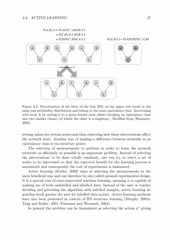
A problem in learning BN structures is that factorization of the joint probabil-ity using Equation 3.1 can lead to the exactly same result for several differentnetworks. In other words, there can be more than one network coding the sameindependence assumptions between variables. The set of network structuresthat produce the same factorization is called an equivalence class. An exampleis given in Figure 3.2. The equivalency of networks can easily be checked graph-ically since two DAGs are equivalent if they have the same structure ignoringedge directions (called skeleton of the graph) and the same v-structures (a nodewith two non-adjacent parents) (Verma and Pearl, 1991). Equivalence classesare in fact a manifestation of the well-known saying that correlation does notimply causation.

Equivalence classes lead to the problem that in learning the network structureseveral different DAGs are score-equivalent and, consequently, one is able to onlydistinguish between equivalence classes but not the DAGs inside them. However,as shown in Figure 3.2, one can break these classes by making interventions, i.e.

3.4. ACTIVE LEARNING 27

A"

C"

B" A"

C"

B" A"

C"

B" A"

C"

B"

( , , ) ( ) ( | ) ( | )( ) ( | ) ( | )( ) ( | ) ( | )

P A B C P A P C A P B CP C P A C P B CP B P C B P A C

=

=

= ),|()()(),,( BACPBPAPCBAP =

A"

C"

B" A"

C"

B" A"

C"

B"

interven+on"on"A"

Figure 3.2: Factorization of the three of the four BNs on the upper row result in thesame join probability distribution and belong to the same equivalence class. Interveningwith node A by setting it to a given known state allows breaking an equivalence classinto two smaller classes (of which the other is a singleton). Modified from (Husmeier,2005).

setting values for certain nodes and then observing how those interventions affectthe network state. Another way of making a difference between networks in anequivalence class is via structure priors.

The selection of measurements to perform in order to learn the networkstructure as efficiently as possible is an important problem. Instead of selectingthe interventions to be done totally randomly, one can try to select a set ofnodes to be intervened so that the expected benefit for the learning process ismaximized and consequently the cost of experiments is minimized.

Active learning (Settles, 2009) aims at selecting the measurements in themost beneficial way and can therefore be also called optimal experimental design.It is a special case of semi-supervised machine learning, meaning it is capable ofmaking use of both unlabelled and labelled data. Instead of the user or teacherdeciding and providing the algorithm with labelled samples, active learning al-gorithm itself queries the user for labelled data points. Active learning methodshave also been presented in context of BN structure learning (Murphy, 2001a;Tong and Koller, 2001; Pournara and Wernisch, 2004).

In general the problem can be formulated as selecting the action a

⇤ giving


the maximal expected utility, as defined by function F (a), i.e.

a

⇤ = argmaxa2A

F (a), (3.16)

where the set A consists of all the possible actions. The actions can be for exam-ple perturbations of nodes in the network before measurement, as in PublicationII. In this case the expected utility was defined as

F (a) =X

G2G

X

y2YG,a

P (y|G, a,D)P (G|D)U (G, a, y,D), (3.17)

where G is the set of possible DAGs and YG,a denotes the set of possible ob-servations that G can produce given that perturbation a has been made. Forthe utility function U(G, a, y,D) we use (assuming equivalent cost for each in-tervention) logP (G|a, y,D) (Murphy, 2001a). Due to the super-exponentiallygrowing number of DAGs and the large amount of different possible states YG,a

the network can take, computational complexity increases so that in trying toselect the action maximizing Equation 3.16, one must use sampling instead ofexhaustive evaluation with networks having more than about 6 nodes.

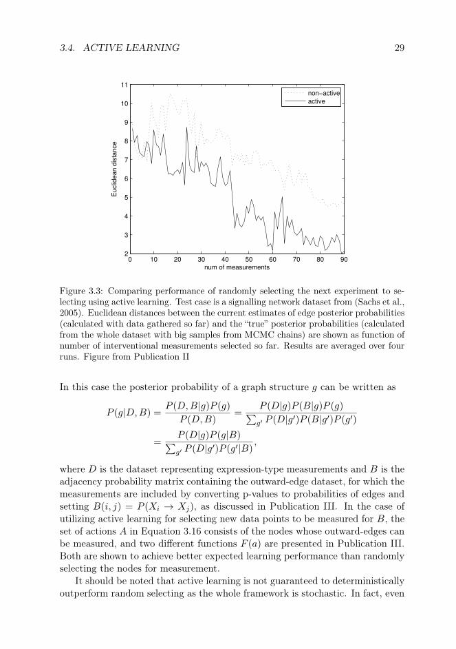
Publication II presents and benchmarks this active learning algorithm intwo realistic cases with actual experimental data. The first dataset consistsof expression measurements of 7 transcription factor genes in Halobacteriumsalinarum, including both wild-type measurements as well as over-expressions.The second one contains flow cytometry measurements of 11 signalling networkproteins, of which for 5 the dataset includes perturbation measurements (Sachset al., 2005). Active learning is found to perform on average more efficientlythan randomly selecting the measurements (or interventions) to perform, seeFigure 3.3 for an example. However, the performance is not quite as good aswith simulated data, which has most often been used to assess the methods.Reasons for lower average performance, although still better than when selectingperturbations randomly, are likely at least factors outside the model affecting themeasured nodes and cyclic regulatory relationships not captured by BNs.

Publication III discusses how to apply active learning in a scenario withheterogeneous datatypes by means of using structure priors. There can oftenexist multiple types of measurement data from the same biological system andincluding those in the inference of network structure can be done with BNs, byincorporating part of the data through likelihoods and the rest via structurepriors. We concentrated on a biologically motivated setting, where one datatypecontains measurements of the states of network nodes, e.g. gene expression mea-surements, whereas the other datatype can be used to measure the probabilitiesof outward-edges for nodes, such as done in for example ChIP-seq measurements.

3.4. ACTIVE LEARNING 29

0 10 20 30 40 50 60 70 80 902

3

4

5

6

7

8

9

10

11

num of measurements

Euclidean d

ista

nce

non−active

active

Figure 3.3: Comparing performance of randomly selecting the next experiment to se-lecting using active learning. Test case is a signalling network dataset from (Sachs et al.,2005). Euclidean distances between the current estimates of edge posterior probabilities(calculated with data gathered so far) and the “true” posterior probabilities (calculatedfrom the whole dataset with big samples from MCMC chains) are shown as function ofnumber of interventional measurements selected so far. Results are averaged over fourruns. Figure from Publication II

In this case the posterior probability of a graph structure g can be written as

P (g|D,B) =P (D,B|g)P (g)

P (D,B)=

P (D|g)P (B|g)P (g)P

g0 P (D|g0)P (B|g0)P (g0)

=P (D|g)P (g|B)

P

g0 P (D|g0)P (g0|B),

where D is the dataset representing expression-type measurements and B is theadjacency probability matrix containing the outward-edge dataset, for which themeasurements are included by converting p-values to probabilities of edges andsetting B(i, j) = P (Xi ! Xj), as discussed in Publication III. In the case ofutilizing active learning for selecting new data points to be measured for B, theset of actions A in Equation 3.16 consists of the nodes whose outward-edges canbe measured, and two different functions F (a) are presented in Publication III.Both are shown to achieve better expected learning performance than randomlyselecting the nodes for measurement.

It should be noted that active learning is not guaranteed to deterministicallyoutperform random selecting as the whole framework is stochastic. In fact, even


worse performance can at times be observed, even though on average activelearning yields beneficial results.

Chapter 4

Modeling metabolic networks

Metabolites interact with each other, being able to combine into new metabo-lites, exchange molecules, or break apart. This process of interactions is naturallydescribed as a network, where nodes represent metabolites and edges the inter-actions between them. Constructing such descriptions or models of metabolism(often called reconstructions or genome-scale models (GEMs) of metabolism)usually starts by identifying genes that code for known metabolic enzymes inthe genome of the organism being studied. Finding out the functions of genesis initially done by homology search and sometimes followed by manual or ex-perimental curation. The rapidly reduced cost of genome sequencing has greatlylowered the threshold of obtaining such annotated (even though often just draft)genomes.

Given a list of enzymes assumed to be present in the cell, one has implicitlyalso a list of metabolites and possible interactions between them. However, theselists are still most likely incomplete, as even the most studied genomes are notthoroughly annotated, and the lists are also prone to contain erroneous items,due to for example inadequacy of homology to resolve functional proteins andindependence of some reactions (like transfer/exchange) on enzymes. As anexample of a well-curated but still incompletely annotated organism one mightconsider human and its metabolic reconstruction, which still in the latest versionapproximately doubled the numbers of both metabolites and reactions (Thieleet al., 2013).

Knowledge of the reactions catalyzed by the set of enzymes allows additionof stoichiometric coefficients to the model, revealing how many molecules of eachmetabolite take part in one interaction step. Some reactions are also thermo-dynamically feasible in only other direction and this directionality informationshould also be included.

The well-known central dogma of molecular biology (Crick, 1958) states thatthe information flow is directed from gene to RNA to protein. Based on this,rules can be generated for reactions in a reconstruction stating whether the

31

32 CHAPTER 4. MODELING METABOLIC NETWORKS

enzyme (which is a protein) needed for the reaction to take place is availablewithin the cell. Thus, in the most basic setting, if gene G codes for RNA R,which is transcribed to enzyme E, then from expression of G it can be deducedthat the reaction catalyzed by E can take place.

Complications with this simple model of gene-enzyme connection arise inmany fronts. First, the relationship between gene expression and protein levelsis far from being simple (Vogel and Marcotte, 2012). Another level of complexityarises in eukaryotic cells, where a single gene can produce multiple transcripts,which in turn can each produce multiple different proteins as depicted in Figure4.1. In addition, many enzymes are protein complexes being built from multiple(different) proteins. Therefore the reconstructions may contain gene-protein-reaction association rules that state in Boolean formalism the required states ofgenes in order for the reaction to be able to occur. This information about thegene-reaction associations is essential in using metabolic models for predictingphenotypic effects in for example knock-out mutants.

Figure 4.1: The synthesis principle of proteins in an eukaryotic cell. G denotes a gene,Ti are the different splice variants and Pi the resulting proteins after post-translationalmodifications.

The above description of the process of building (called reconstruction of)metabolic networks is oversimplified. However, the way to make metabolic re-constructions is quite established (Feist et al., 2009; Thiele and Palsson, 2010)and many advanced tools for the task exist (Karp et al., 2010; Thorleifsson andThiele, 2011; Schellenberger et al., 2011; Pabinger et al., 2014).

Since the first genome-scale metabolic reconstruction in Edwards and Pals-son (1999), over a hundred published reconstructions have appeared (Feist et al.,2009; InSilicoOrganisms, 2009). Some of the most studied and well-developedones include E. coli (Feist et al., 2007; Orth et al., 2011) and S. cerevisiae (Moet al., 2009). Also for some widely-studied organisms, the reconstructions haverecently been developed and improved in a community-driven effort, such asfor human (Thiele et al., 2013) and yeast (Herrgård et al., 2008). However,investigation of the reconstructions reveals that there is still much room for im-

4.1. CONSTRAINT-BASED MODELS 33

provement, for example in that many model mainly only the primary metabolism(Monk et al., 2014).

4.1 Constraint-based models

The structure of metabolic networks can be studied using graph theoretic meth-ods but here we are more interested in the flow (or, more precisely, fluxes) ofmetabolites through the network. Even though kinetic information for the ma-jority of reactions is unknown and absent from the models described above, theconstraints set by the models (such as structural, stoichiometric and thermody-namic ones) limit the allowed functioning of the metabolic network and studyingthe resulting flux space is insightful and can yield accurate predictions. Studyingthe models built given the structure and constraints is called constraint-basedmodelling (Bordbar et al., 2014). In the following, we shortly review basic con-cepts in characterization of the set of all possible flux distributions, which hasalso been called metabolic pathway analysis (Schilling et al., 1999). See also(Schuster et al., 2002) for a good description of the matters discussed below.

In a system of m metabolites and r possible reactions between these metabo-lites, the reaction rates at a given time t can be described as a vector v(t) =[v1(t), v2(t), . . . , vr(t)]

T , where vi(t) is the reaction rate of the ith reaction. Vec-tor v is often called flux distribution (we drop the notation t wherever it is betterfor readability).

Each of the reactions is either reversible or irreversible. The direction isdefined by thermodynamic constraints so that even though a reaction might inreality be able to proceed in both directions, it is still classified as irreversible ifunder the prevailing conditions it can only happen in the other direction. Basedon these, a flux distribution v can be divided into subvectors vrev and virr

containing the reversible and irreversible reactions, respectively, and now we can

write v =

vrev

virr

�

. The directions of the irreversible reactions are defined to

satisfyvirr � 0. (4.1)

System boundary modelling can be done in at least two ways, as shown inFigure 4.2. First, it is possible to define some reactions as transfer reactions ca-pable of bringing a metabolite to the system or removing it from there (i.e. theyare one-ended edges across the system boundary). The other way is to catego-rize metabolites to be either internal or external. In the first category all thereactions having influence on the concentration of the metabolite are includedin the studied model, while in the latter one not all the reactions with an effecton the metabolite are included in the model and their concentration is assumedconstant (sometimes called source or sink metabolites).


A"

B"

C"

F"D"

E"

C"

D"E"

Figure 4.2: Two alternative views for modelling system boundaries. In the left figurethe dashed nodes represent external metabolites and the nodes with solid lines areinternal metabolites. In the figure on the right hand-side dashed lines denote exchangeor transfer reactions. The grey lines depict the system boundaries.

The network structure and stoichiometric coefficients (which define the quan-tity of a molecule taking part in a reaction) of the system can be described by anm⇥ r stoichiometric matrix S. Now, we can define the system to be in steady-state if all the metabolites i are being consumed at the same rate as they arebeing produced, i.e.

dXi

dt

=X

j

Si,jvj = 0, (4.2)

where Xi is the concentration of metabolite i. Thus, for the whole system

Sv = 0, (4.3)

which can be attained (at least approximately) by many biochemical systems insuitable stable conditions, such as in some chemostat cultivations.

Equations 4.3 and 4.1 together define the allowed part of the flux space wherethe system can be given the constraints. If we first look at Equation 4.3, we seethat the vectors v satisfying it form a null-space (also called kernel) of S, i.e.K = null(S) = {v 2 Rr : Sv = 0}.

If all the reactions in the network are reversible, then the limits of themetabolic capabilities can be defined as the linear basis of the null-space. Usuallythis is not the case, and the irreversibility constraints of Equation 4.1 restrictthe null-space into an allowed sub-space, namely every element in virr definesa half-space in the null-space. The result is a convex polyhedral cone, which isreferred to as the flux cone. This is illustrated in Figure 4.3.

In addition to the above constraints, the flux cone can also be defined bythe vectors that form its edges and these vectors are called extreme rays orgenerating vectors (Gagneur and Klamt, 2004). They unambiguously define thecone, much like a set of basis vectors, except that they are not necessarily linearlyindependent.

There are two different but closely related approaches for identifying fluxesthat are close to being generating vectors. These are elementary modes (EM)(Schuster et al., 2000) and extreme pathways (EP) (Schilling et al., 1999;


Figure 4.3: A flux cone in the space of three fluxes. The arrows forming the edges ofthe cone are the generating vectors.

Schilling et al., 2000). See for example (Klamt and Stelling, 2003) for a reviewand comparison of both.

Intuitively, both EMs and EPs represent a minimal set of fluxes (or path-ways) whose superposition can be used to achieve any feasible steady-state ofthe network. For example in case of EMs

v =X

j

↵jej , (4.4)

where ↵j 2 R,↵j � 0, and ej is the jth EM of the network in consideration.This property means that the EMs give the limits of the metabolic network andwork as its basis (although not linearly independent). An example of a networkand its elementary modes is shown in Figure 4.4.

Both EM and EP methods are seriously limited by combinatorial explosion,which has resulted them being mostly of theoretical interest while flux balanceanalysis, which is presented in the next subsection, is the main tool used. How-ever, there are also developments that characterize the flux cone much moreefficiently (Larhlimi and Bockmayr, 2009; Rezola et al., 2011).

Some methods aim at characterizing the flux distributions based on experi-mental data, such as measurements of nutrient uptake rates or isotope labellingdata. Such methods can be called Metabolic Flux Analysis (MFA) (Wiechert,2001) or Metabolic Network Analysis (MNA) (Christensen and Nielsen, 2000).Including such data basically further constraints the flux space and thus en-ables the estimation of intracellular fluxes in greater detail. The possibility ofobtaining such data is limited, e.g., due to difficulties in labeling the substrates


EM1

EM3

EM2

EM4

Figure 4.4: An example network on top. Below are its four elementary modes denotedin black. Metabolites A, G and H are external.

and in addition mass spectrometry or nuclear magnetic resonance techniques arerequired for the measurements.

As the majority of biochemical reactions are mediated by enzymes, whichare proteins coded by genes, it is natural that information about genes and theirexpression states is utilized in metabolic network modelling. The informationabout connection between genes and reactions is often existing as result of thereconstruction of metabolic network being based on identified enzyme-codinggenes, as described above. However, factors complicating this task are that geneexpression values cannot in general be taken as surrogates for protein concentra-tion or expression values as this connection has been shown to be only moderate(Greenbaum et al., 2003; Vogel and Marcotte, 2012) and that transcriptionalregulation has been found insufficient to explain flux changes (Chubukov et al.,2013).

Thus, even though the effect of gene regulation is reduction in the spaceof steady-state solutions (Covert et al., 2001b; Covert and Palsson, 2003) andincluding this extra information in the modelling should in principle make theresults more accurate (and indeed has, e.g., (Covert et al., 2001b; Covert etal., 2004; Lerman et al., 2013)), the combination of metabolic and gene modelsis not easy. For a survey on the methods integrating transcriptomic data toconstraint-based models see, e.g., (Machado and Herrgård, 2014).


4.1.1 Flux balance analysis

The goal of flux balance analysis (FBA) (Varma and Palsson, 1994; Kauffmanet al., 2003; Raman and Chandra, 2009) is to find a particular optimal fluxdistribution given the same constraints as discussed above, i.e. the result is asingle point in the flux cone. The optimal solution v is one that minimizes (ormaximizes) an objective function. This can be stated as a linear programmingproblem where v is subject to the mass balance (steady-state) constraint Sv = 0and constraints on the magnitudes of reactions ↵i vi �i. The objectivefunction is defined as

Z =X

i

ci · vi = cTv, (4.5)

where vector c selects the desired set of fluxes and gives them the weights foroptimization. For example, if one wants to find the maximal cellular growthrate, then c is defined so that it contains each of the requirements of growth incorrect relation to others, which can be found out experimentally for exampleby studying the composition of biomass.

The use of an objective function can be justified from the principle thatevolution drives organisms to function optimally. Then the selection of objectivefunction should follow biological reality as well as possible in order to make theresults meaningful. Finding such an aim for a complex cell type in a complicatedand evolving environment can be close to impossible. For a simple organism, suchas a bacterium, the main aim is often to grow as fast as possible. Then, a sensibleobjective to be maximized is the growth function and results of FBA using thishave been found to closely follow experimental results (Edwards et al., 2001).

However, there are conditions and phenotypes where simple growth objectivefunction clearly does not hold. Several different objective functions can be triedin such conditions (Schuetz et al., 2007). It has also been noted that, for exam-ple in predicting knock-outs, the straight-forward maximization of the objectivefunction (even if it is correct) might not be ideal due to, e.g., limited evolution-ary time (Segre et al., 2002). Also, it is unlikely that the metabolism of a cellcan be characterized sufficiently using only the formalism of FBA together witha suitably chosen objective function, as for example variations in gene activitiesoften have effects on metabolism.

Problems with FBA might arise with the alternate optimal solutions, i.e. thepossible existence of infinitely many solutions resulting the exactly same optimalvalue of the objective function (Mahadevan and Schilling, 2003). This can causeproblems in situations where something else is of interest than the functionbeing maximized in FBA. For example, in trying to predict hydrogen yield,the maximization of biomass might be possible when hydrogen gets any valuewithin some given constraints and is thus not uniquely determined. An approachin which this is often solved is to first run FBA maximizing biomass production,then fix biomass to this value and use FBA again with objective function being


on the flux of interest.Flux balance analysis (and constraint-based methods in general) have been

shown to perform well when compared to experimental results, see e.g. (Edwardset al., 2001; Famili et al., 2003; Feist et al., 2007) and correct prediction ratesof more than 80% have been achieved (Duarte et al., 2004) when predicting via-bility in knock-out experiments. However, the accuracy of predictions is highlydependent on the coverage and quality of the metabolic reconstruction and howwell the phenomenon at hand can be approximated given the assumptions ofFBA.

Computationally FBA is easy to solve as it is a simple optimization problemsolvable by linear programming. Thus, as a method it is easily implemented andsolved on most of the current programming languages (using an external solver ifneeded). There are also software tools developed that can perform FBA analysis(including FBA-SimVis (Grafahrend-Belau et al., 2009), CycSim (Le Fèvre et al.,2009), BioMet Toolbox (Cvijovic et al., 2010), COBRA toolbox (Schellenbergeret al., 2011), and others (Lakshmanan et al., 2014)), some of which also offervisualizations and other analysis possibilities.

Flux balance analysis has been applied for already quite long, e.g., in mod-elling (Jørgensen et al., 1995; Edwards et al., 2001), predicting drug targets(Folger et al., 2011; Oberhardt et al., 2013), and metabolic engineering (Liaoet al., 1996) due to the possibility to aid in redesigning the network for overpro-duction of a desired substance (Burgard et al., 2003; Pharkya et al., 2004; Broet al., 2006).

In Publication IV, the accuracy of predicting yields of a specific metabolite(hydrogen) in E. coli was studied in anaerobic batch-cultures that are suitablefor screening beneficial mutations but challenge in particular the steady-stateassumption of FBA as well as the used metabolic reconstruction, which was de-veloped for and tested on mostly aerobic conditions (Feist et al., 2007). Thedata against which the predictions were compared was obtained by gas chro-matography and optical density measurements. Although the performance ofFBA in predicting viability of mutants is also in this case rather good (⇠78%),predicting the yields was found to be much more difficult, with only 33% of thecases with predicted increase in hydrogen production yielding increase experi-mentally. Reasons for the encountered discrepancies were likely due to imperfectreconstruction and in particular its unsuitability to model anaerobic conditions.Also the differences in alternate metabolic intake (glucose vs. galactose) werefound to be not captured by the model, where modelling the phosphotransferasesystem and its regulation would be needed. Despite the differences in predictedyields, computational predictions are valuable in screening out cases that showno change so that they can be omitted in further investigation.

It is noted that modifications to FBA that may be better suited for knock-out(or perturbed) mutants have been presented. One approach, called minimization


of metabolic adjustment (MOMA) (Segre et al., 2002), does not calculate theoptimum value for knock-out mutants but instead a projection of the wild-typeoptimal value to the feasible space of the knock-out mutant, which in general isnot the same as the optimal result obtained via FBA. A closely related approach,named regulatory on/off minimization (ROOM) (Shlomi et al., 2005), minimizesthe number of significant alterations of fluxes in the knock-out mutant whencompared to the wild-type. Both of these approaches are based on the ideathat a knock-out mutant has not had enough time to evolve into optimality, asrequired by FBA, but instead the flux configuration of the mutant strain liesclose to the wild-type one without in general being optimal. Investigating theperformance of these models in the same scenario would be interesting in thefuture.

In Publication V, FBA was used as a part of a model aiming to simulatethe interplay between chemotactic movement of a population of E. coli cellsand substrate concentration in the environment. FBA was used to model themetabolic state of each individual bacterium of the population given the con-centration of the substrates in the environment. As the environmental stateand consequently the metabolic state of the bacteria evolve over a time-course,the modelling was done by simply dividing the time into intervals and assuming(pseudo-)steady-state within each interval, which is sometimes called dynamicflux balance analysis (Mahadevan et al., 2002). The state of the environment isthen updated based on the uptake rates of the bacteria.

Chapter 5

Summary of the results

Identification of interacting entities, such as genes or proteins, and the networksthey form is one of the key targets in many biological studies. These networkscan be inferred and modelled using several different formalisms, one of which isBayesian networks. Learning the structure of BNs gets complicated because ofthe huge model-space even at low numbers of nodes in the network. Therefore itis often done by using some way of approximating or sampling, such as generatinga sample from the posterior distribution of the space of network structures asdone with Markov Chain Monte Carlo.

One of the main problems related to MCMC is the rate of convergence tothe actual target distribution. This can be to some extent tackled with modifiedproposal distributions but an issue when constructing them in the context ofBayesian networks is that their structure is restricted to directed acyclic graphs(DAGs).

In Publication I, a modification to MCMC for BN structure learning is pre-sented that allows efficient movements to larger than the standard single-stepneighbourhoods in the DAG space, which is achieved by using composite pro-posal distributions consisting of one or more single-step transitions. The methodis compared to the standard one that proposes only single-step transitions usinga big dataset of about 5,400 datapoints, each containing the states of 11 sig-nalling network proteins measured using flow-cytometry. The standard methodis noted to have serious difficulties in convergence while the method presentedin Publication I is shown to improve convergence by avoiding the MCMC chainsgetting stuck to local maxima and increasing computational demands only verylittle. The possibility to tune the proportions of different length transitions isalso demonstrated and it is shown that a mixture of for example one- and two-step transitions seems to produce the best outcome in this application. Thus,the method increases the possibility of finding the correct network structure fora given biological system.

As the causal relationships are usually of ultimate interest in studying bio-

41

42 CHAPTER 5. SUMMARY OF THE RESULTS

logical systems, it is necessary to introduce interventions to the studied systems.Bayesian networks can readily handle interventional data together with obser-vational data but they can also be used to predict which interventions would bebeneficial to perform in order to learn the structure of the network with max-imum efficiency. This is called active learning and Publication II investigateshow such methods perform in comparison with normal, “non-active” learning,with two different sets of real measurement data. One dataset consists of ex-pression measurements from seven transcription factor genes of a bacterium, andthe other dataset is the same signalling protein dataset as used in Publication I.Both test cases show that active learning does on average produce better resultsin the sense that fewer measurements are needed to get to the same accuracy ofresults.

However, in these cases with real data the improvements of active versusrandom learning can be relatively modest, whereas the gap between the twohas been wider for most studies where simulated datasets have been used. Onereason why the improvement is not so dramatic in the presented cases is that thereal underlying biological systems are usually not acyclic and thus cannot fullybe modelled using Bayesian networks, whereas the simulated datasets are usuallygenerated from a BN. Another reason is that although the simulated data alsohas a certain level of uncertainties, the noise is likely much more prevalent inactual measurements.

Publication III presents an active learning method for Bayesian networks,where the measurement data subject to active learning selection is incorporatedvia structure priors. In addition, other data without active learning selection isincluded through likelihoods as normally. Since the structure priors define beliefsin different structures and therefore edges in the network, the most naturalmeasurements to be included using them are for example such that somehowmeasure more directly the interactions between entities, denoted in PublicationIII as binding data.

In the first test case with simulated gene regulatory networks, binding datawould correspond to, e.g., ChIP-seq data, which can be used to quantify bindingof the product of a gene to the promoter (or another regulatory element) of atarget gene. In the other test case the same signalling protein network as previ-ously was used, in which case the real binding data could come from some wayof quantifying protein-protein interactions. Due to lack of suitable measurementdatasets, the binding measurements were simulated in Publication III. Again,active learning is shown on average to outperform randomly selecting the mea-surements to be done. Taken together, Publications II and III demonstrate thatactive learning methods are potentially very useful in biological research becauseof their ability to reduce the amount of required experiments, which are oftentedious and expensive to carry out.

A computational network model for one of the best-known and most widely-

43

used bacterium, Escherichia coli, is used in Publication IV to predict effects ofsingle gene knock-outs on the amount of hydrogen produced by the bacterium.The used model was a well-developed version based on whole-genome data andthe predictions of the metabolic network performance for all different knock-outsavailable were made using flux balance analysis. Predictions were also made withtwo other methods: (1) based on an algorithm looking at reactions that competefor precursors of hydrogen and (2) selecting knock-outs manually.

The knock-outs giving highest yields of hydrogen were selected and the corre-sponding mutants were then ordered and cultivated, and the measured biomassand hydrogen productions were compared to the predicted values. Viability,as determined by the ability to produce biomass, was correct in about 78% ofcases. However, increased hydrogen production was observed in only 33% of thecases predicted to have increased yield. One reason for the relatively bad pre-diction accuracy is that the metabolic model is primarily developed and testedunder aerobic conditions whereas the cultivations were in anaerobic conditions.Another reason is that batch cultures do not necessarily attain a steady-state,which is the assumption underlying FBA. Even if the cells at some point in theculture are in a steady-state, the end-point measurements made in PublicationIV represent a mixture of all the states and thus might not give a correct pictureof the steady-state performance.

Part of the discrepancies between measurements and predictions - in partic-ular for viability predictions, i.e. formation of biomass - can also be explainedby difficulties in defining the growth media completely in FBA since the usedcasamino acids included in the growth medium contain several of the essentialamino acids. The metabolic reconstructions are usually not tested and developedin such complex growth media and thus might not correctly take into account theuptakes and usage routes of extracellular amino acids, which may be the reasonbehind some of the erroneous predictions. The use of metabolic models for mak-ing predictions to guide in engineering organisms for production of substances isanyhow a useful tool in evaluating potential usefulness of the mutations and inparticular the viability of the mutants.

In Publication V, the simulation of metabolic network of E. coli is com-bined with a model for its chemotactic network and environmental substrateconcentration. For a single bacterium, one submodel simulates the chemotacticnetwork response as a function of the extracellular aspartate concentration andthe resulting changes in the swimming behaviour, and the other submodel simu-lates the effect of metabolism on both the external aspartate concentration andgrowth of the bacterium using flux balance analysis. Even though the bacteriaare independent, they depend on each other indirectly by influencing their sharedenvironment by creating concentration gradients which redirect the movementsof the (sub)populations.

The modelling is done in a state-based and executable framework, which is

44 CHAPTER 5. SUMMARY OF THE RESULTS

convenient in that for example states of bacteria (running/tumbling) are natu-rally handled and that the executable components can be easily run indepen-dently and created or destroyed dynamically. In Publication V, the modelledpopulation sizes were small (⇠100 bacteria) and further development is clearlyneeded.

Chapter 6

Conclusions

Inference of structure of many networks is a task needed in several fields andapplications. For example, advanced methods for measuring activities of allthe genes of an organism have become available within the last decades. Suchdatasets in effect represent measurements of thousands of variables at a timeand trying to, for example, find the network structure explaining the data is nota trivial problem. In Publication I, an improvement to one specific inferenceproblem has been presented, which improves the performance of the standardmethod for learning the structure of a Bayesian network. Besides increased rateof convergence, the method is also flexible and allows, e.g., adjustments to bedone based on the dataset. The potential next steps could include studyingadaptive MCMC schemes for BN structure learning.

Limiting the use of static Bayesian networks is the requirement for acyclicityof the structure, which in biological systems is clearly not justified due to theubiquitous feed-back loops that have been observed. However, even though oneBN structure might not be the biologically correct one, it is still possible tofind the interactions with high posterior probabilities. In fact, often one is notnecessarily so interested in the maximum a posteriori network but instead it ismore useful to calculate posterior probabilities over certain features based ona sample from the posterior distribution, which is the rationale behind MCMCand thus also Publication I. The usability of Bayesian networks is also restrictedby the huge size of structure-space, making them unusable for genome scaleanalyses or necessitating other modifications, such as dividing the problem intomanageable-sized subparts, to be used.

In order to guarantee that the inferred relationships between entities of thenetwork are causal, it is necessary to introduce interventions to the system andmeasure the effects of them. Selecting those interventions and/or measurementsthat maximally increase our knowledge about the network structure, thereforealso making inference as fast and efficient as possible, is a problem tackled byactive learning methods. As presented in Publications II and III, active learning

45

46 CHAPTER 6. CONCLUSIONS

improves learning on average.For many complex systems it is generally not possible to get enough infor-

mation using only one data type and several different “views” into the systemare instead used to measure various aspects. Therefore, the ability to integrateseveral different data types into the same inference framework is very benefi-cial, as done in Publication III. In the same publication, the ability of activelearning in the context of Bayesian networks is shown to improve efficiency ofstructure learning also when the data is included via priors. Further study onthe subject could include investigating cost functions that allow suggesting mea-surements from more than one data type by balancing the cost of performinga measurement and expected benefit from receiving the result of the measure-ment. Moreover, improvements in the computational efficiency of the methodsare necessary in order to allow applications to larger systems. The method couldalso be updated to utilize the calculation of exact edge posterior probabilities(Koivisto and Sood, 2004).

Biological organisms are increasingly being used in producing substances ofinterest as well as for degrading unwanted substances. As all wanted metaboliccapabilities are rarely available in a single organism or the desired end-productsmight be consumed by the organism itself, metabolic engineering needs to beperformed to modify existing cells. Simplest forms of such modifications areknock-outs and computationally predicting their effect on metabolism would beextremely beneficial. As presented in Publication IV, the state of the methodsdoes not completely allow doing this, highlighting the difficulty of capturingbiological complexity in a model. Still, modelling offers an invaluable way tonarrow down the list of possibilities in deciding which modifications to make,even though there is plenty of room for improvements.

In the future, it could be interesting to study the predictability under dif-ferent growth conditions (such as chemostat cultures) and using for exampledynamic flux balance analysis given that time-course measurements would beavailable. Performing the experiments in a much simpler growth medium wouldalso be sensible, which probably would allow the models to fit the experimentaldata better. Besides FBA, the utility of other methods, such as MOMA (Segreet al., 2002) and ROOM (Shlomi et al., 2005), should in addition be evaluated.None of the methods has been reported to produce best results consistently, soa reasonable test could be to use them all in a kind of ensemble approach to se-lect the most promising candidate mutations. The performance of the methodsfor predicting more than single-gene deletions or additions would be interest-ing to study, as usually modifying only single gene might not give considerableimprovements.

Often biological systems are studied not as a whole due to the very highcomplexity. Instead, focus is more on certain subsystems, for which highly de-veloped and accurate models may have been built. An example of such separate

47

subsystems are metabolism and chemotaxis in E. coli. Integration of submodelsis of importance because certain responses and behaviours can only arise as thecombined action of all of them. The chemotaxis model presented in PublicationV is able to integrate both metabolic and signalling network models into an ex-ecutable model that can give rise to behaviour at population-level as a result oftheir interplay via the state of environment. The presented approach, Biocharts,also allows easily producing predictions and further hypotheses as the model isbasically a program and its subprogram parameters are easily modified. Includ-ing some recent advances in stochastic models of chemotaxis has been done afterthe publication, which allows simulations of much larger populations of bacteria,thus getting closer to numbers in real biological assays.

In the future it would be interesting and rather easy to extend the model forscenarios with multiple substrates for which the bacteria have varying prefer-ences, thereby generating several subpopulations as also shown in experiments.However, limitations set by the incapabilities of metabolic and chemotactic mod-els correctly taking into account uptakes and effects of other substrates is likelya major problem.

Computational analysis and mathematical modelling of biological phenom-ena are arguably needed more than ever nowadays, and their importance is likelyto increase in the future. All the models suffer from being incomplete and areto varying extent unable to make accurate predictions, necessitating further de-velopments. This thesis has addressed some of the issues related to learning andsimulation of the models, and has hopefully taken some small steps in the pathtowards increased applicability of the models.

Bibliography

Adler, J. (1966), “Chemotaxis in Bacteria”, Science, 153 (3737): 708–716.Adler, J. (1975), “Chemotaxis in Bacteria”, Annual Review of Biochemistry ,

44 (1): 341–356.Äijö, T. and Lähdesmäki, H. (2009), “Learning Gene Regulatory Networks

from Gene Expression Measurements Using Non-Parametric Molecular Ki-netics”, Bioinformatics , 25 (22): 2937–2944.

Allison, D. B., Cui, X., Page, G. P., and Sabripour, M. (2006), “Microar-ray Data Analysis: From Disarray to Consolidation and Consensus”, NatureReviews Genetics, 7 (1): 55–65.

Andrews, S. S. (2012), “Spatial and Stochastic Cellular Modeling with theSmoldyn Simulator”, in: Bacterial Molecular Networks, Springer: pp. 519–542.

Andrews, S. S. and Arkin, A. P. (2006), “Simulating Cell Biology”, CurrentBiology , 16 (14): R523–R527.

Andrews, S. S. and Bray, D. (2004), “Stochastic Simulation of Chemical Reac-tions with Spatial Resolution and Single Molecule Detail”, Physical Biology ,1 (3): 137–151.

Armitage, J. P. (1999), “Bacterial Tactic Responses”, Advances in MicrobialPhysiology , 41: 229–289.

Bansal, M., Belcastro, V., Ambesi-Impiombato, A., and Bernardo, D.di (2007), “How to Infer Gene Networks from Expression Profiles”, MolecularSystems Biology , 3: 78.

Barabasi, A.-L. (2002), Linked: How Everything Is Connected to EverythingElse and What It Means, Plume Editors.

Barabasi, A.-L. and Oltvai, Z. N. (2004), “Network Biology: Understandingthe Cell’s Functional Organization”, Nature Reviews Genetics , 5 (2): 101–113.

Beaumont, M. A. and Rannala, B. (2004), “The Bayesian Revolution inGenetics”, Nature Reviews Genetics , 5 (4): 251–261.

Berg, H. C. and Brown, D. A. (1972), “Chemotaxis in Escherichia coli Anal-ysed by Three-Dimensional Tracking”, Nature, 239 (5374): 500–504.

49

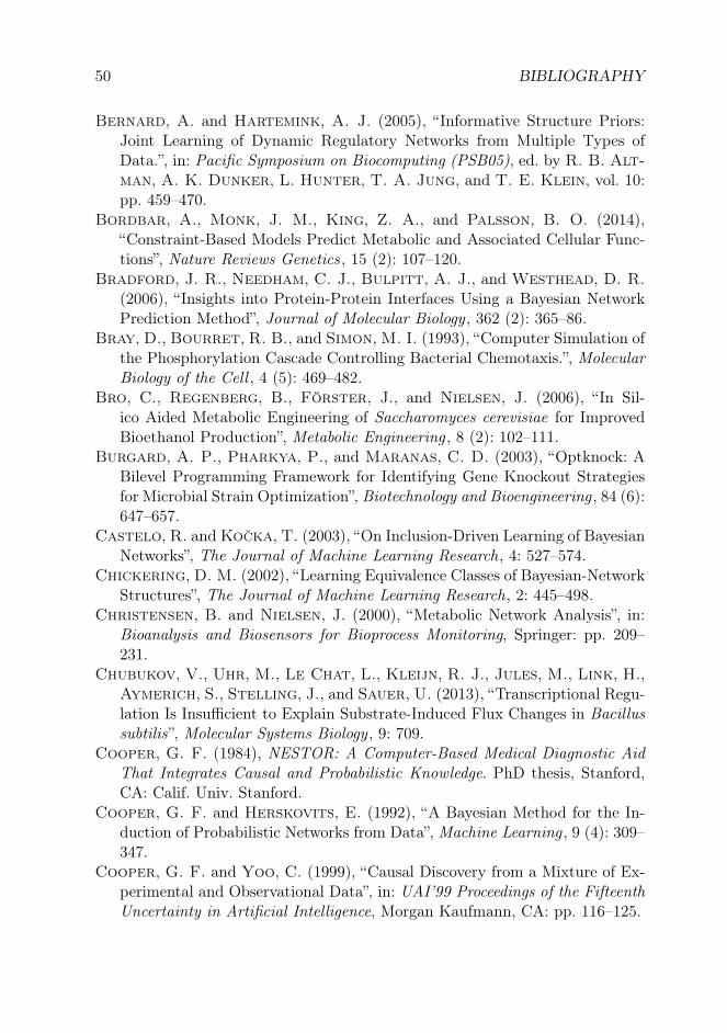
50 BIBLIOGRAPHY

Bernard, A. and Hartemink, A. J. (2005), “Informative Structure Priors:Joint Learning of Dynamic Regulatory Networks from Multiple Types ofData.”, in: Pacific Symposium on Biocomputing (PSB05), ed. by R. B. Alt-man, A. K. Dunker, L. Hunter, T. A. Jung, and T. E. Klein, vol. 10:pp. 459–470.

Bordbar, A., Monk, J. M., King, Z. A., and Palsson, B. O. (2014),“Constraint-Based Models Predict Metabolic and Associated Cellular Func-tions”, Nature Reviews Genetics , 15 (2): 107–120.

Bradford, J. R., Needham, C. J., Bulpitt, A. J., and Westhead, D. R.(2006), “Insights into Protein-Protein Interfaces Using a Bayesian NetworkPrediction Method”, Journal of Molecular Biology , 362 (2): 365–86.

Bray, D., Bourret, R. B., and Simon, M. I. (1993), “Computer Simulation ofthe Phosphorylation Cascade Controlling Bacterial Chemotaxis.”, MolecularBiology of the Cell , 4 (5): 469–482.

Bro, C., Regenberg, B., Förster, J., and Nielsen, J. (2006), “In Sil-ico Aided Metabolic Engineering of Saccharomyces cerevisiae for ImprovedBioethanol Production”, Metabolic Engineering , 8 (2): 102–111.

Burgard, A. P., Pharkya, P., and Maranas, C. D. (2003), “Optknock: ABilevel Programming Framework for Identifying Gene Knockout Strategiesfor Microbial Strain Optimization”, Biotechnology and Bioengineering , 84 (6):647–657.

Castelo, R. and Koc̆ka, T. (2003), “On Inclusion-Driven Learning of BayesianNetworks”, The Journal of Machine Learning Research, 4: 527–574.

Chickering, D. M. (2002), “Learning Equivalence Classes of Bayesian-NetworkStructures”, The Journal of Machine Learning Research, 2: 445–498.

Christensen, B. and Nielsen, J. (2000), “Metabolic Network Analysis”, in:Bioanalysis and Biosensors for Bioprocess Monitoring, Springer: pp. 209–231.

Chubukov, V., Uhr, M., Le Chat, L., Kleijn, R. J., Jules, M., Link, H.,Aymerich, S., Stelling, J., and Sauer, U. (2013), “Transcriptional Regu-lation Is Insufficient to Explain Substrate-Induced Flux Changes in Bacillussubtilis”, Molecular Systems Biology , 9: 709.

Cooper, G. F. (1984), NESTOR: A Computer-Based Medical Diagnostic AidThat Integrates Causal and Probabilistic Knowledge. PhD thesis, Stanford,CA: Calif. Univ. Stanford.

Cooper, G. F. and Herskovits, E. (1992), “A Bayesian Method for the In-duction of Probabilistic Networks from Data”, Machine Learning , 9 (4): 309–347.

Cooper, G. F. and Yoo, C. (1999), “Causal Discovery from a Mixture of Ex-perimental and Observational Data”, in: UAI’99 Proceedings of the FifteenthUncertainty in Artificial Intelligence, Morgan Kaufmann, CA: pp. 116–125.

BIBLIOGRAPHY 51

Covert, M. W. and Palsson, B. O. (2003), “Constraints-Based Models: Regu-lation of Gene Expression Reduces the Steady-State Solution Space”, Journalof Theoretical Biology , 221 (3): 309–325.

Covert, M. W., Schilling, C. H., Famili, I., Edwards, J. S., Goryanin,I. I., Selkov, E., and Palsson, B. O. (2001a), “Metabolic Modeling ofMicrobial Strains in silico”, Trends in Biochemical Sciences, 26 (3): 179–186.

Covert, M. W., Schilling, C. H., and Palsson, B. (2001b), “Regulation ofGene Expression in Flux Balance Models of Metabolism”, Journal of Theo-retical Biology , 213 (1): 73–88.

Covert, M. W., Knight, E. M., Reed, J. L., Herrgard, M. J., and Pals-son, B. O. (2004), “Integrating High-Throughput and Computational DataElucidates Bacterial Networks”, Nature, 429 (6987): 92–96.

Cowell, R. G., Dawid, A. P., Lauritzen, S. L., and Spiegelhalter, D. J.(1999), Probabilistic Networks and Expert Systems, New York: Springer.

Cowles, M. K. and Carlin, B. P. (1996), “Markov Chain Monte Carlo Con-vergence Diagnostics: A Comparative Review”, Journal of the American Sta-tistical Association, 91 (434): 883–904.

Crick, F. H. (1958), “On Protein Synthesis”, in: Symposia of the Society forExperimental Biology, vol. 12: p. 138.

Cvijovic, M., Olivares-Hernández, R., Agren, R., Dahr, N., Vongsang-nak, W., Nookaew, I., Patil, K. R., and Nielsen, J. (2010), “BioMetToolbox: Genome-Wide Analysis of Metabolism”, Nucleic Acids Research,38 (suppl 2): W144–W149.

De Jong, H. (2002), “Modeling and Simulation of Genetic Regulatory Systems:A Literature Review”, Journal of Computational Biology , 9 (1): 67–103.

Demir, E., Cary, M. P., Paley, S., Fukuda, K., Lemer, C., Vastrik, I.,Wu, G., D’Eustachio, P., Schaefer, C., Luciano, J., et al. (2010), “TheBioPAX Community Standard for Pathway Data Sharing”, Nature Biotech-nology , 28 (9): 935–942.

Dempster, A. P., Laird, N. M., and Rubin, D. B. (1977), “Maximum Like-lihood from Incomplete Data Via the EM Algorithm”, Journal of the RoyalStatistical Society. Series B (Methodological), 39 (1): 1–38.

Diaconis, P. (2009), “The Markov Chain Monte Carlo Revolution”, Bulletin ofthe American Mathematical Society , 46 (2): 179–205.

Dojer, N., Bednarz, P., Podsiadlo, A., and Wilczynski, B. (2013), “BN-Finder2: Faster Bayesian Network Learning and Bayesian Classification”,Bioinformatics , 29 (16): 2068–70.

Duarte, N. C., Herrgård, M. J., and Palsson, B. Ø. (2004), “Reconstruc-tion and Validation of Saccharomyces cerevisiae IND750, a Fully Compart-mentalized Genome-Scale Metabolic Model”, Genome Research, 14 (7): 1298–1309.

52 BIBLIOGRAPHY

Eaton, D. and Murphy, K. (2007a), “Bayesian Structure Learning Using Dy-namic Programming and MCMC”, in: UAI 2007, Proceedings of the Twenty-Third Conference on Uncertainty in Artificial Intelligence, Vancouver, BC,Canada: Morgan Kaufmann, CA: pp. 101–108.

Eaton, D. and Murphy, K. (2007b), “Exact Bayesian Structure Learningfrom Uncertain Interventions”, in: Proceedings of the Eleventh InternationalConference on Artificial Intelligence and Statistics, San Juan, Puerto Rico:pp. 107–114.

Eaton, D. and Murphy, K. (2007c), BDAGL: Bayesian DAG Learning, http://www.cs.ubc.ca/~murphyk/Software/BDAGL/.

Eddy, S. R. (2004), “What Is Bayesian Statistics?”, Nature Biotechnology ,22 (9): 1177–1178.

Edwards, J. S., Ibarra, R. U., and Palsson, B. O. (2001), “In silico Pre-dictions of Escherichia coli Metabolic Capabilities Are Consistent with Ex-perimental Data”, Nature Biotechnology , 19 (2): 125–130.

Edwards, J. S. and Palsson, B. O. (1999), “Systems Properties of theHaemophilus influenzae Rd Metabolic Genotype”, Journal of BiologicalChemistry , 274 (25): 17410–17416.

Elf, J. and Ehrenberg, M. (2004), “Spontaneous Separation of Bi-Stable Bio-chemical Systems into Spatial Domains of Opposite Phases”, Systems Biol-ogy , 1 (2): 230–236.

Ellis, B. and Wong, W. H. (2008), “Learning Causal Bayesian Network Struc-tures from Experimental Data”, Journal of the American Statistical Associ-ation, 103 (482): 778–789.

Emonet, T., Macal, C. M., North, M. J., Wickersham, C. E., andCluzel, P. (2005), “AgentCell: A Digital Single-Cell Assay for BacterialChemotaxis”, Bioinformatics , 21 (11): 2714–2721.

Famili, I., Förster, J., Nielsen, J., and Palsson, B. O. (2003), “Saccha-romyces cerevisiae Phenotypes Can Be Predicted by Using Constraint-BasedAnalysis of a Genome-Scale Reconstructed Metabolic Network”, Proceedingsof the National Academy of Sciences, 100 (23): 13134–13139.

Fang, Z. and Cui, X. (2011), “Design and Validation Issues in RNA-seq Exper-iments”, Briefings in Bioinformatics, bbr004.

Feist, A. M., Henry, C. S., Reed, J. L., Krummenacker, M., Joyce, A.R., Karp, P. D., Broadbelt, L. J., Hatzimanikatis, V., and Palsson,B. Ø. (2007), “A Genome-Scale Metabolic Reconstruction for Escherichiacoli K-12 MG1655 That Accounts for 1260 ORFs and Thermodynamic In-formation”, Molecular Systems Biology , 3: 121.

Feist, A. M., Herrgård, M. J., Thiele, I., Reed, J. L., and Palsson,B. Ø. (2009), “Reconstruction of Biochemical Networks in Microorganisms”,Nature Reviews Microbiology , 7 (2): 129–143.

BIBLIOGRAPHY 53

Fisher, J. and Henzinger, T. A. (2007), “Executable Cell Biology”, NatureBiotechnology , 25 (11): 1239–1249.

Folger, O., Jerby, L., Frezza, C., Gottlieb, E., Ruppin, E., and Shlomi,T. (2011), “Predicting Selective Drug Targets in Cancer Through MetabolicNetworks”, Molecular Systems Biology , 7: 501.

Friedman, N., Linial, M., Nachman, I., and Pe’er, D. (2000), “UsingBayesian Networks to Analyze Expression Data”, Journal of ComputationalBiology , 7 (3-4): 601–620.

Friedman, N. (2004), “Inferring Cellular Networks Using Probabilistic Graph-ical Models”, Science, 303 (5659): 799–805.

Friedman, N. and Koller, D. (2003), “Being Bayesian About Network Struc-ture – a Bayesian Approach to Structure Discovery in Bayesian Networks”,Machine Learning , 50 (1-2): 95–125.

Friedman, N., Murphy, K., and Russell, S. (1998), “Learning the Struc-ture of Dynamic Probabilistic Networks”, in: Proceedings of the FourteenthConference on Uncertainty in Artificial Intelligence, UAI’98, Madison, Wis-consin: Morgan Kaufmann Publishers Inc.: pp. 139–147.

Gagneur, J. and Klamt, S. (2004), “Computation of Elementary Modes: AUnifying Framework and the New Binary Approach”, BMC Bioinformatics,5 (1): 175.

Geiger, D. and Heckerman, D. (1998), “A Characterization of the BivariateWishart Distribution”, Probability and Mathematical Statistics, 18 (1): 119–131.

Ghahramani, Z. (1998), “Learning Dynamic Bayesian Networks”, in: AdaptiveProcessing of Sequences and Data Structures, Springer: pp. 168–197.

Gillespie, D. T. (1976), “A General Method for Numerically Simulating theStochastic Time Evolution of Coupled Chemical Reactions”, Journal of Com-putational Physics, 22 (4): 403–434.

Gillespie, D. T. (1977), “Exact Stochastic Simulation of Coupled ChemicalReactions”, The Journal of Physical Chemistry , 81 (25): 2340–2361.

Giudici, P. and Castelo, R. (2003), “Improving Markov Chain Monte CarloModel Search for Data Mining”, Machine Learning , 50 (1-2): 127–158.

Good, I. J. (1961), “A Causal Calculus (I)”, The British Journal for the Phi-losophy of Science, 11 (44): 305–318.

Grafahrend-Belau, E., Klukas, C., Junker, B. H., and Schreiber, F.(2009), “FBA-SimVis: Interactive Visualization of Constraint-Based MetabolicModels”, Bioinformatics , 25 (20): 2755–2757.

Greenbaum, D., Colangelo, C., Williams, K., and Gerstein, M. (2003),“Comparing Protein Abundance and mRNA Expression Levels on a GenomicScale”, Genome Biology , 4 (9): 117.

54 BIBLIOGRAPHY

Grzegorczyk, M. and Husmeier, D. (2008), “Improving the StructureMCMC Sampler for Bayesian Networks by Introducing a New Edge ReversalMove”, Machine Learning , 71 (2-3): 265–305.

Haario, H., Laine, M., Mira, A., and Saksman, E. (2006), “DRAM: EfficientAdaptive MCMC”, Statistics and Computing , 16: 339–354.

Harel, D. (1987), “Statecharts: A Visual Formalism for Complex Systems”,Science of Computer Programming , 8 (3): 231–274.

Harel, D. and Gery, E. (1996), “Executable Object Modeling with State-charts”, in: Proceedings of the 18th International Conference on SoftwareEngineering, IEEE Computer Society: pp. 246–257.

Hartemink, A. J., Gifford, D. K., Jaakkola, T. S., and Young, R. A.(2002), “Combining Location and Expression Data for Principled Discoveryof Genetic Regulatory Network Models”, in: Pacific Symposium on Biocom-puting, vol. 7: pp. 437–449.

Hartemink, A. J. (2001), Principled Computational Methods for the Validationand Discovery of Genetic Regulatory Networks. PhD thesis, MIT.

Hastings, W. K. (1970), “Monte Carlo Sampling Methods Using MarkovChains and Their Applications”, Biometrika, 57 (1): 97–109.

Heckerman, D. (1998), “A Tutorial on Learning with Bayesian Networks”,English, in: Learning in Graphical Models, ed. by M. Jordan, vol. 89, NATOASI Series, Springer Netherlands: pp. 301–354.

Heckerman, D., Geiger, D., and Chickering, D. M. (1995a), “LearningBayesian Networks: The Combination of Knowledge and Statistical Data”,Machine Learning , 20 (3): 197–243.

Heckerman, D., Mamdani, A., and Wellman, M. P. (1995b), “Real-WorldApplications of Bayesian Networks”, Communications of the ACM , 38 (3):24–26.

Herrgård, M. J., Swainston, N., Dobson, P., Dunn, W. B., Arga, K. Y.,Arvas, M., Blüthgen, N., Borger, S., Costenoble, R., Heinemann,M., et al. (2008), “A Consensus Yeast Metabolic Network ReconstructionObtained from a Community Approach to Systems Biology”, Nature Biotech-nology , 26 (10): 1155–1160.

Hucka, M., Finney, A., Sauro, H. M., Bolouri, H., Doyle, J. C., Kitano,H., Arkin, A. P., Bornstein, B. J., Bray, D., Cornish-Bowden, A.,et al. (2003), “The Systems Biology Markup Language (SBML): A Mediumfor Representation and Exchange of Biochemical Network Models”, Bioinfor-matics, 19 (4): 524–531.

Husmeier, D. (2005), Probabilistic Modeling in Bioinformatics and MedicalInformatics. In: ed. by D. Husmeier, R. Dybowski, and S. Roberts,Springer Berlin Heidelberg, chap. Introduction to Learning Bayesian Net-works from Data: pp. 17–57.

BIBLIOGRAPHY 55

InSilicoOrganisms, Available Predictive Genome-Scale Metabolic Network Re-constructions, http://gcrg.ucsd.edu/InSilicoOrganisms/OtherOrganisms.

Jansen, R., Yu, H., Greenbaum, D., Kluger, Y., Krogan, N. J., Chung,S., Emili, A., Snyder, M., Greenblatt, J. F., and Gerstein, M. (2003),“A Bayesian Networks Approach for Predicting Protein-Protein Interactionsfrom Genomic Data”, Science, 302 (5644): 449–53.

Johnson, D. S., Mortazavi, A., Myers, R. M., and Wold, B. (2007),“Genome-Wide Mapping of in Vivo Protein-DNA Interactions”, Science,316 (5830): 1497–1502.

Jørgensen, H., Nielsen, J., Villadsen, J., and Møllgaard, H. (1995),“Metabolic Flux Distributions in Penicillium chrysogenum During Fed-BatchCultivations”, Biotechnology and Bioengineering , 46 (2): 117–131.

Karlebach, G. and Shamir, R. (2008), “Modelling and Analysis of Gene Reg-ulatory Networks”, Nature Reviews Molecular Cell Biology , 9 (10): 770–780.

Karp, P. D., Paley, S. M., Krummenacker, M., Latendresse, M., Dale,J. M., Lee, T. J., Kaipa, P., Gilham, F., Spaulding, A., Popescu, L.,et al. (2010), “Pathway Tools Version 13.0: Integrated Software for Path-way/genome Informatics and Systems Biology”, Briefings in Bioinformatics,11 (1): 40–79.

Kauffman, K. J., Prakash, P., and Edwards, J. S. (2003), “Advances inFlux Balance Analysis”, Current Opinion in Biotechnology , 14 (5): 491–496.

Kauffman, S. A. (1969), “Metabolic Stability and Epigenesis in RandomlyConstructed Genetic Nets”, Journal of Theoretical Biology , 22 (3): 437–467.

Kitano, H., Funahashi, A., Matsuoka, Y., and Oda, K. (2005), “UsingProcess Diagrams for the Graphical Representation of Biological Networks”,Nature Biotechnology , 23 (8): 961–966.

Klamt, S. and Stelling, J. (2003), “Two Approaches for Metabolic PathwayAnalysis?”, TRENDS in Biotechnology , 21 (2): 64–69.

Kohn, K. W., Aladjem, M. I., Weinstein, J. N., and Pommier, Y. (2006),“Molecular Interaction Maps of Bioregulatory Networks: A General Rubricfor Systems Biology”, Molecular Biology of the Cell , 17 (1): 1–13.

Koivisto, M. and Sood, K. (2004), “Exact Bayesian Structure Discovery inBayesian Networks”, Journal of Machine Learning Research, 5: 549–573.

Kugler, H. (2013), “Biocharts: Unifying Biological Hypotheses with Modelsand Experiments”, in: EScience (eScience), 2013 IEEE 9th InternationalConference On, IEEE: pp. 317–325.

Lähdesmäki, H. and Shmulevich, I. (2008), “Learning the Structure of Dy-namic Bayesian Networks from Time Series and Steady State Measurements”,Machine Learning , 71 (2-3): 185–217.

Lakshmanan, M., Koh, G., Chung, B. K., and Lee, D.-Y. (2014), “SoftwareApplications for Flux Balance Analysis”, Briefings in Bioinformatics, 15 (1):108–122.

56 BIBLIOGRAPHY

Larhlimi, A. and Bockmayr, A. (2009), “A New Constraint-Based Descrip-tion of the Steady-State Flux Cone of Metabolic Networks”, Discrete AppliedMathematics , 157 (10): 2257–2266.

Le Fèvre, F., Smidtas, S., Combe, C, Durot, M, d’Alché-Buc, F., andSchachter, V (2009), “CycSim—an Online Tool for Exploring and Ex-perimenting with Genome-Scale Metabolic Models”, Bioinformatics , 25 (15):1987–1988.

Le Novere, N. and Shimizu, T. S. (2001), “STOCHSIM: Modelling of Stochas-tic Biomolecular Processes”, Bioinformatics , 17 (6): 575–576.

Le Novere, N., Hucka, M., Mi, H., Moodie, S., Schreiber, F., Sorokin,A., Demir, E., Wegner, K., Aladjem, M. I., Wimalaratne, S. M., etal. (2009), “The Systems Biology Graphical Notation”, Nature Biotechnology ,27 (8): 735–741.

Lerman, J. A., Chang, R. L., Hyduke, D. R., Palsson, B. Ø., et al. (2013),“Genome-Scale Models of Metabolism and Gene Expression Extend and Re-fine Growth Phenotype Prediction”, Molecular Systems Biology , 9: 693.

Lewis, T. G. (2011), Network Science: Theory and Applications, John Wiley &Sons.

Liao, J. C., Hou, S.-Y., and Chao, Y.-P. (1996), “Pathway Analysis, Engineer-ing, and Physiological Considerations for Redirecting Central Metabolism”,Biotechnology and Bioengineering , 52 (1): 129–140.

Lindley, D. V. (2000), “The Philosophy of Statistics”, Journal of the RoyalStatistical Society: Series D , 49 (3): 293–337.

Lloyd, C. M., Halstead, M. D., and Nielsen, P. F. (2004), “CellML: ItsFuture, Present and Past”, Progress in Biophysics and Molecular Biology ,85 (2): 433–450.

Loew, L. M. and Schaff, J. C. (2001), “The Virtual Cell: A Software Environ-ment for Computational Cell Biology”, TRENDS in Biotechnology , 19 (10):401–406.

Lok, L. and Brent, R. (2005), “Automatic Generation of Cellular ReactionNetworks with Moleculizer 1.0”, Nature Biotechnology , 23 (1): 131–136.

Machado, D. and Herrgård, M. (2014), “Systematic Evaluation of Meth-ods for Integration of Transcriptomic Data into Constraint-Based Models ofMetabolism”, PLoS Computational Biology , 10 (4): e1003580.

Madigan, D. and York, J. (1995), “Bayesian Graphical Models for DiscreteData”, International Statistical Review , 63 (2): 215–232.

Mahadevan, R and Schilling, C. (2003), “The Effects of Alternate OptimalSolutions in Constraint-Based Genome-Scale Metabolic Models”, MetabolicEngineering , 5 (4): 264–276.

Mahadevan, R., Edwards, J. S., and Doyle III, F. J. (2002), “DynamicFlux Balance Analysis of Diauxic Growth in Escherichia coli”, BiophysicalJournal , 83 (3): 1331–1340.

BIBLIOGRAPHY 57

Margolin, A. A., Nemenman, I., Basso, K., Wiggins, C., Stolovitzky,G., Favera, R. D., and Califano, A. (2006), “ARACNE: An Algorithm forthe Reconstruction of Gene Regulatory Networks in a Mammalian CellularContext”, BMC Bioinformatics, 7 (Suppl 1): S7.

Metropolis, N., Rosenbluth, A. W., Rosenbluth, M. N., Teller, A. H.,and Teller, E. (1953), “Equation of State Calculations by Fast ComputingMachines”, The Journal of Chemical Physics, 21 (6): 1087–1092.

Meyers, S. and Friedland, P. (1984), “Knowledge-Based Simulation ofGenetic Regulation in Bacteriophage Lambda”, Nucleic Acids Research,12 (1Part1): 1–9.

Mo, M. L., Palsson, B. Ø., and Herrgård, M. J. (2009), “Connecting Ex-tracellular Metabolomic Measurements to Intracellular Flux States in Yeast”,BMC Systems Biology , 3 (1): 37.

Mogilner, A., Wollman, R., and Marshall, W. F. (2006), “QuantitativeModeling in Cell Biology: What Is It Good For?”, Developmental Cell , 11 (3):279 –287.

Monk, J., Nogales, J., and Palsson, B. O. (2014), “Optimizing Genome-Scale Network Reconstructions”, Nature Biotechnology , 32 (5): 447–452.

Moore, A. W. and Wong, W.-K. (2003), “Optimal Reinsertion: A New SearchOperator for Accelerated and More Accurate Bayesian Network StructureLearning”, in: Proceedings of the Twentieth International Conference on Ma-chine Learning, ed. by T. Fawcett and N. Mishra, AAAI Press: pp. 552–559.

Mortazavi, A., Williams, B. A., McCue, K., Schaeffer, L., and Wold,B. (2008), “Mapping and Quantifying Mammalian Transcriptomes by RNA-Seq”, Nature Methods, 5 (7): 621–628.

Morton-Firth, C. J. and Bray, D. (1998), “Predicting Temporal Fluctua-tions in an Intracellular Signalling Pathway”, Journal of Theoretical Biology ,192 (1): 117–128.

Morton-Firth, C. J., Shimizu, T. S., and Bray, D. (1999), “A Free-Energy-Based Stochastic Simulation of the Tar Receptor Complex”, Journal of Molec-ular Biology , 286 (4): 1059–1074.

Mukherjee, S. and Speed, T. P. (2008), “Network Inference Using InformativePriors”, Proceedings of the National Academy of Sciences, 105 (38): 14313–14318.

Murata, T. (1989), “Petri Nets: Properties, Analysis and Applications”, Pro-ceedings of the IEEE , 77 (4): 541–580.

Murphy, K. (2001a), Active Learning of Causal Bayes Net Structure, tech. rep.,Department of Computer Science, U.C. Berkeley.

Murphy, K. (2001b), “The Bayes Net Toolbox for Matlab”, Computing Scienceand Statistics, 33 (2): 1024–1034.

58 BIBLIOGRAPHY

Murphy, K. (2013), Software Packages for Graphical Models, http://people.cs.ubc.ca/~murphyk/Software/bnsoft.html.

Murphy, K. and Mian, S. (1999), Modelling Gene Expression Data Using Dy-namic Bayesian Networks, tech. rep. 104, University of California, Berkeley,CA: Computer Science Division.

Myers, C. L., Robson, D., Wible, A., Hibbs, M. A., Chiriac, C., Theesfeld,C. L., Dolinski, K., and Troyanskaya, O. G. (2005), “Discovery of Bio-logical Networks from Diverse Functional Genomic Data”, Genome Biology ,6 (13): R114.

Niinimäki, T. and Koivisto, M. (2013), “Annealed Importance Sampling forStructure Learning in Bayesian Networks”, in: Proceedings of the Twenty-Third International Joint Conference on Artificial Intelligence, AAAI Press:pp. 1579–1585.

Noor, A., Serpedin, E., Nounou, M., Nounou, H., Mohamed, N., andChouchane, L. (2013), “An Overview of the Statistical Methods Used forInferring Gene Regulatory Networks and Protein-Protein Interaction Net-works”, Advances in Bioinformatics , 2013.

Oberhardt, M. A., Yizhak, K., and Ruppin, E. (2013), “Metabolically Re-Modeling the Drug Pipeline”, Current Opinion in Pharmacology , 13 (5): 778–785.

Orth, J. D., Conrad, T. M., Na, J., Lerman, J. A., Nam, H., Feist, A. M.,and Palsson, B. Ø. (2011), “A Comprehensive Genome-Scale Reconstruc-tion of Escherichia coli Metabolism”, Molecular Systems Biology , 7: 535.

Pabinger, S., Snajder, R., Hardiman, T., Willi, M., Dander, A., andTrajanoski, Z. (2014), “MEMOSys 2.0: An Update of the BioinformaticsDatabase for Genome-Scale Models and Genomic Data”, Database, 2014:bau004.

Pearl, J. (1985), “Bayesian Networks: A Model of Self-Activated Memory forEvidential Reasoning”, in: Proceedings of the 7th Conference of the CognitiveScience Society, University of California, Irvine: pp. 329–334.

Pearl, J. (2009), Causality: Models, Reasoning and Inference, 2nd edition,Cambridge University Press.

Pease, A. C., Solas, D., Sullivan, E. J., Cronin, M. T., Holmes, C. P.,and Fodor, S. (1994), “Light-generated Oligonucleotide Arrays for RapidDNA Sequence Analysis”, Proceedings of the National Academy of Sciences,91 (11): 5022–5026.

Pharkya, P., Burgard, A. P., and Maranas, C. D. (2004), “OptStrain: AComputational Framework for Redesign of Microbial Production Systems”,Genome Research, 14 (11): 2367–2376.

Pournara, I. and Wernisch, L. (2004), “Reconstruction of Gene NetworksUsing Bayesian Learning and Manipulation Experiments”, Bioinformatics ,20 (17): 2934–2942.

BIBLIOGRAPHY 59

Quach, M., Brunel, N., and d’Alché-Buc, F. (2007), “Estimating Parame-ters and Hidden Variables in Non-Linear State-Space Models Based on ODEsfor Biological Networks Inference”, Bioinformatics , 23 (23): 3209–3216.

Raman, K. and Chandra, N. (2009), “Flux Balance Analysis of BiologicalSystems: Applications and Challenges”, Briefings in Bioinformatics, 10 (4):435–449.

Ren, B., Robert, F., Wyrick, J. J., Aparicio, O., Jennings, E. G., Simon,I., Zeitlinger, J., Schreiber, J., Hannett, N., Kanin, E., et al. (2000),“Genome-Wide Location and Function of DNA Binding Proteins”, Science,290 (5500): 2306–2309.

Rezola, A., Figueiredo, L. F. de, Brock, M, Pey, J., Podhorski, A.,Wittmann, C., Schuster, S., Bockmayr, A., and Planes, F. J. (2011),“Exploring Metabolic Pathways in Genome-Scale Networks Via GeneratingFlux Modes”, Bioinformatics , 27 (4): 534–540.

Robinson, R. W. (1977), “Counting Unlabeled Acyclic Digraphs”, in: Proceed-ings of the Fifth Australian Conference on Combinatorial Mathematics, ed.by C. Little, Springer, Berlin.

Rousseau, W. F. (1968), A Method for Computing Probabilities in ComplexSituations. Tech. rep., Center for Systems Research, Stanford University.

Sachs, K., Perez, O., Pe’er, D., Lauffenburger, D. A., and Nolan, G.P. (2005), “Causal Protein-Signaling Networks Derived from MultiparameterSingle-Cell Data”, Science, 308 (5721): 523–529.

Schellenberger, J., Que, R., Fleming, R. M., Thiele, I., Orth, J. D.,Feist, A. M., Zielinski, D. C., Bordbar, A., Lewis, N. E., Rahma-nian, S., et al. (2011), “Quantitative Prediction of Cellular Metabolism withConstraint-Based Models: The COBRA Toolbox V2. 0”, Nature Protocols,6 (9): 1290–1307.

Schena, M., Shalon, D., Davis, R. W., and Brown, P. O. (1995), “Quanti-tative Monitoring of Gene Expression Patterns with a Complementary DNAMicroarray”, Science, 270 (5235): 467–470.

Schilling, C. H., Letscher, D., and Palsson, B. Ø. (2000), “Theory forthe Systemic Definition of Metabolic Pathways and Their Use in Interpret-ing Metabolic Function from a Pathway-Oriented Perspective”, Journal ofTheoretical Biology , 203 (3): 229–248.

Schilling, C. H., Schuster, S., Palsson, B. O., and Heinrich, R. (1999),“Metabolic Pathway Analysis: Basic Concepts and Scientific Applications inthe Post-Genomic Era”, Biotechnology Progress, 15 (3): 296–303.

Schuetz, R., Kuepfer, L., and Sauer, U. (2007), “Systematic Evaluation ofObjective Functions for Predicting Intracellular Fluxes in Escherichia coli”,Molecular Systems Biology , 3: 119.

60 BIBLIOGRAPHY

Schuster, S., Fell, D. A., and Dandekar, T. (2000), “A General Definitionof Metabolic Pathways Useful for Systematic Organization and Analysis ofComplex Metabolic Networks”, Nature Biotechnology , 18 (3): 326–332.

Schuster, S., Hilgetag, C., Woods, J. H., and Fell, D. A. (2002), “Re-action Routes in Biochemical Reaction Systems: Algebraic Properties, Val-idated Calculation Procedure and Example from Nucleotide Metabolism”,Journal of Mathematical Biology , 45: 153–181.

Segal, E., Barash, Y., Simon, I., Friedman, N., and Koller, D. (2002),“From Promoter Sequence to Expression: A Probabilistic Framework”, in:Proceedings of the Sixth Annual International Conference on ComputationalBiology, ACM: pp. 263–272.

Segre, D., Vitkup, D., and Church, G. M. (2002), “Analysis of Optimalityin Natural and Perturbed Metabolic Networks”, Proceedings of the NationalAcademy of Sciences , 99 (23): 15112–15117.

SEQC/MAQC-III Consortium (2014), “A Comprehensive Assessment ofRNA-seq Accuracy, Reproducibility and Information Content by the Se-quencing Quality Control Consortium”, Nature Biotechnology , 32 (9): 903–914.

Settles, B. (2009), Active Learning Literature Survey, Computer SciencesTechnical Report 1648, University of Wisconsin–Madison.

Setty, Y., Cohen, I. R., Dor, Y., and Harel, D. (2008), “Four-DimensionalRealistic Modeling of Pancreatic Organogenesis”, Proceedings of the NationalAcademy of Sciences , 105 (51): 20374–20379.

Setty, Y., Dalfó, D., Korta, D. Z., Hubbard, E. J. A., and Kugler, H.(2012), “A Model of Stem Cell Population Dynamics: In Silico Analysis andin Vivo Validation”, Development , 139: 47–56.

Shlomi, T., Berkman, O., and Ruppin, E. (2005), “Regulatory On/Off Mini-mization of Metabolic Flux Changes After Genetic Perturbations”, Proceed-ings of the National Academy of Sciences, 102 (21): 7695–7700.

Shmulevich, I., Dougherty, E. R., Kim, S., and Zhang, W. (2002), “Prob-abilistic Boolean Networks: A Rule-Based Uncertainty Model for Gene Reg-ulatory Networks”, Bioinformatics , 18 (2): 261–274.

Slepchenko, B. M. and Loew, L. M. (2010), “Use of Virtual Cell in Studiesof Cellular Dynamics”, International Review of Cell and Molecular Biology ,283: 1–56.

Smith, V. A., Yu, J., Smulders, T. V., Hartemink, A. J., and Jarvis, E.D. (2006), “Computational Inference of Neural Information Flow Networks”,PLoS Computational Biology , 2 (11): e161.

Tamada, Y., Kim, S., Bannai, H., Imoto, S., Tashiro, K., Kuhara, S., andMiyano, S. (2003), “Estimating Gene Networks from Gene Expression Databy Combining Bayesian Network Model with Promoter Element Detection”,Bioinformatics , 19 Suppl 2: ii227–ii236.

BIBLIOGRAPHY 61

Thar, R. and Kühl, M. (2003), “Bacteria Are Not Too Small for Spatial Sens-ing of Chemical Gradients: An Experimental Evidence”, Proceedings of theNational Academy of Sciences, 100 (10): 5748–5753.

Thiele, I. and Palsson, B. Ø. (2010), “A Protocol for Generating a High-Quality Genome-Scale Metabolic Reconstruction”, Nature Protocols, 5 (1):93–121.

Thiele, I., Swainston, N., Fleming, R. M., Hoppe, A., Sahoo, S., Aurich,M. K., Haraldsdottir, H., Mo, M. L., Rolfsson, O., Stobbe, M.D., et al. (2013), “A Community-Driven Global Reconstruction of HumanMetabolism”, Nature Biotechnology , 31 (5): 419–425.

Thorleifsson, S. G. and Thiele, I. (2011), “rBioNet: A COBRA ToolboxExtension for Reconstructing High-Quality Biochemical Networks”, Bioin-formatics, 27 (14): 2009–2010.

Tindall, M. J., Maini, P. K., Porter, S. L., and Armitage, J. P. (2008a),“Overview of Mathematical Approaches Used to Model Bacterial ChemotaxisII: Bacterial Populations”, Bulletin of Mathematical Biology , 70 (6): 1570–1607.

Tindall, M., Porter, S., Maini, P., Gaglia, G, and Armitage, J. (2008b),“Overview of Mathematical Approaches Used to Model Bacterial ChemotaxisI: The Single Cell”, Bulletin of Mathematical Biology , 70 (6): 1525–1569.

Tong, S. and Koller, D. (2001), “Active Learning for Structure in BayesianNetworks”, in: IJCAI’01 Proceedings of the 17th International Joint Con-ference on Artificial Intelligence, vol. 2, Seattle, Washington, USA: MorganKaufmann: pp. 863–869.

Troyanskaya, O. G., Dolinski, K., Owen, A. B., Altman, R. B., andBotstein, D. (2003), “A Bayesian Framework for Combining HeterogeneousData Sources for Gene Function Prediction (in Saccharomyces Cerevisiae)”,Proceedings of the National Academy of Sciences, 100 (14): 8348–53.

Varma, A. and Palsson, B. O. (1994), “Metabolic Flux Balancing: Basic Con-cepts, Scientific and Practical Use”, Nature Biotechnology , 12 (10): 994–998.

Verma, T. and Pearl, J. (1991), “Equivalence and Synthesis of Causal Mod-els”, in: Proceedings of the Sixth Annual Conference on Uncertainty in Ar-tificial Intelligence, UAI ’90, New York, NY, USA: Elsevier Science Inc.:pp. 255–270.

Vogel, C. and Marcotte, E. M. (2012), “Insights into the Regulation ofProtein Abundance from Proteomic and Transcriptomic Analyses”, NatureReviews Genetics, 13 (4): 227–232.

Wadhams, G. H. and Armitage, J. P. (2004), “Making Sense of It All: Bacte-rial Chemotaxis”, Nature Reviews Molecular Cell Biology , 5 (12): 1024–1037.

Werhli, A. V. and Husmeier, D. (2007), “Reconstructing Gene RegulatoryNetworks with Bayesian Networks by Combining Expression Data with Mul-

62 BIBLIOGRAPHY

tiple Sources of Prior Knowledge”, Statistical Applications in Genetics andMolecular Biology , 6 (1).

Werhli, A. V., Grzegorczyk, M., and Husmeier, D. (2006), “Compar-ative Evaluation of Reverse Engineering Gene Regulatory Networks withRelevance Networks, Graphical Gaussian Models and Bayesian Networks”,Bioinformatics , 22 (20): 2523–2531.

Wiechert, W. (2001), “13C Metabolic Flux Analysis”, Metabolic Engineering ,3 (3): 195–206.

Wilczyński, B. and Dojer, N. (2009), “BNFinder: Exact and Efficient Methodfor Learning Bayesian Networks”, Bioinformatics , 25 (2): 286–7.

Wright, S. (1921), “Correlation and Causation”, Journal of Agricultural Re-search, 20 (7): 557–585.

Wu, F.-X., Zhang, W.-J., and Kusalik, A. J. (2004), “Modeling Gene Ex-pression from Microarray Expression Data with State-Space Equations.”, in:Pacific Symposium on Biocomputing, vol. 9: pp. 581–592.

Zhao, W., Serpedin, E., and Dougherty, E. R. (2006), “Inferring GeneRegulatory Networks from Time Series Data Using the Minimum DescriptionLength Principle”, Bioinformatics , 22 (17): 2129–2135.

Zhu, X., Gerstein, M., and Snyder, M. (2007), “Getting Connected: Analysisand Principles of Biological Networks”, Genes & Development , 21 (9): 1010–1024.

Publications

Publication I

A. Larjo and H. Lähdesmäki, “Using multi-step proposal distribution for im-proved MCMC convergence in Bayesian network structure learning,” submittedto EURASIP Journal on Bioinformatics and Systems Biology, 2014.

Publication II

A. Larjo, H. Lähdesmäki, M. Facciotti, N. Baliga, I. Shmulevich, and O. Yli-Harja, “Active learning of Bayesian network structure in a realistic setting,” inFifth International Workshop on Computational Systems Biology (WCSB 2008),Leipzig, Germany, June 11-13, 2008, pp. 85-88.

Publication III

A. Larjo and H. Lähdesmäki, “Active learning for Bayesian network models ofbiological networks using structure priors,” in IEEE International Workshop onGenomic Signal Processing and Statistics, Houston, TX, USA, November 17-19,2013, pp. 78-81.

© 2013 IEEE

Publication IV

J.J. Seppälä*, A. Larjo*, T. Aho, O. Yli-Harja, M.T. Karp, and V. Santala,“Prospecting hydrogen production of Escherichia coli by metabolic network mod-eling,” International Journal of Hydrogen Energy, vol. 38, no. 27, pp. 11780-11789, 2013.

Publication V

H. Kugler*, A. Larjo*, and D. Harel, “Biocharts: A visual formalism for com-plex biological systems,” Journal of the Royal Society Interface, vol. 7, no. 48,pp. 1015–1024, 2010.

computational methods for modelling and analysing ... · computational methods for modelling and...

Documents