Phylogeny-based methods for analysing genomes and metagenomes

Presented by Aaron Darling

OTUs for ecology

Operational Taxonomic Unit: a grouping of similar sequences that can be treated as a single “species”

● Strengths

– Conceptually simple

– Mask effect of poor quality data● Sequencing error● in vitro recombination

● Weaknesses

– Limited resolution

– Logically inconsistent definition

Logical inconsistency: OTUs at 97% ID

A

B

OTU pipelines will arbitrarily pick one of the three solutions.Is this actually a problem??

C

Assume the true phylogeny:

A, B > 97% identityB, C > 97% identityA and C not > 97% ID

Possible valid OTUs:AB, C (with A & C centroids)A, BC (with A & C centroids)ABC (with B centroid)

0.02

0.005

0.005

0.01

Limited resolution

OTU groupingsignore the finestructure presentin phylogeny

Same species, different genomes

Perna et al 2001 Nature, Welch et al 2002 PNAS

Three genomes, same species only 40% genes in common

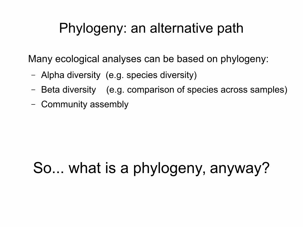
Phylogeny: an alternative path

Many ecological analyses can be based on phylogeny:

– Alpha diversity (e.g. species diversity)

– Beta diversity (e.g. comparison of species across samples)

– Community assembly

So... what is a phylogeny, anyway?

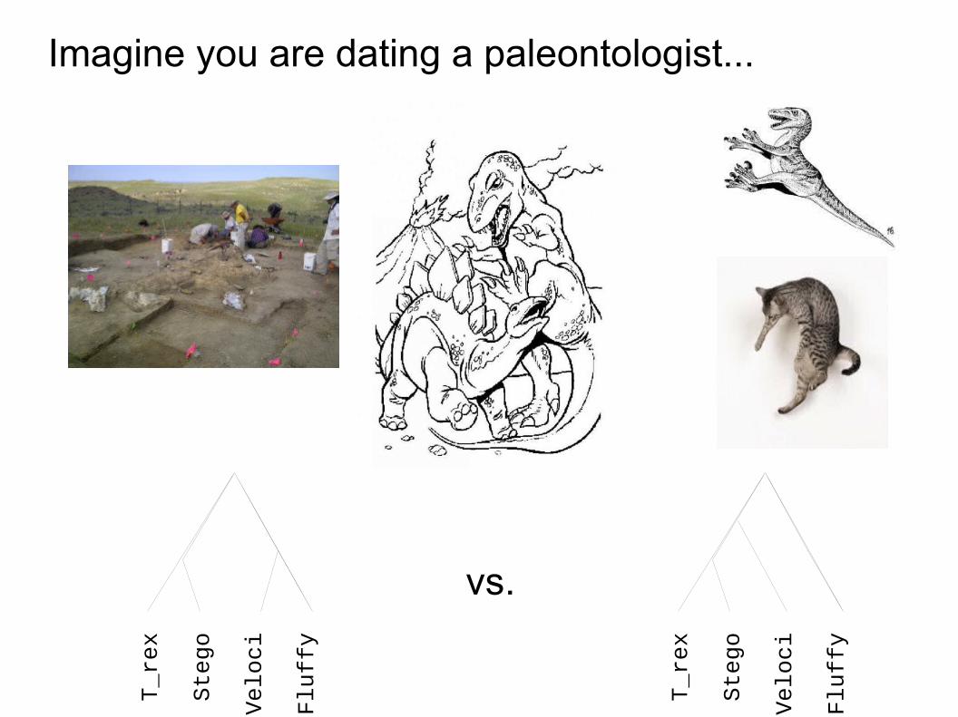
Imagine you are dating a paleontologist...

T_rex

Stego

Veloci

Fluffy

T_rex

Stego

Veloci

Fluffy

vs.

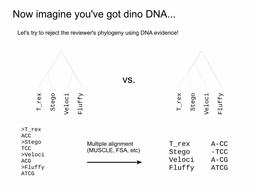
Now imagine you've got dino DNA...

>T_rexACC>StegoTCC>VelociACG>FluffyATCG

T_rex A-CCStego -TCCVeloci A-CGFluffy ATCG

Multiple alignment(MUSCLE, FSA, etc)

T_rex

Stego

Veloci

Fluffy

T_rex

Stego

Veloci

Fluffy

vs.

Let's try to reject the reviewer's phylogeny using DNA evidence!

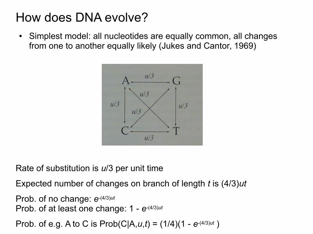
How does DNA evolve?● Simplest model: all nucleotides are equally common, all changes

from one to another equally likely (Jukes and Cantor, 1969)

Rate of substitution is u/3 per unit time

Expected number of changes on branch of length t is (4/3)ut

Prob. of no change: e-(4/3)ut

Prob. of at least one change: 1 - e-(4/3)ut

Prob. of e.g. A to C is Prob(C|A,u,t) = (1/4)(1 - e-(4/3)ut )

Calculating the likelihood of data given a tree

Steps:

1) Branch lengths

2) Finite-time transition probabilities

3) Leaf node partial probabilities

T_rex

Stego

Veloci

Fluffy

A-CC

-TCC

A-CG

ATCG

A 1 1 0 0C 0 1 1 1G 0 1 0 0T 0 1 0 0

A 1 0 0 0C 0 0 1 0G 0 0 0 1T 0 1 0 0

A 1 1 0 0C 0 1 1 0G 0 1 0 1T 0 1 0 0

A 1 0 0 0C 1 0 1 1G 1 0 0 0T 1 1 0 0

1.0 1.0units of time

P(X|Y,u,t) = (1/4)(1 - e-(4/3)ut )

P(X|Y,0.1,1.0) = 0.0312P(X|X,0.1,1.0) = 0.9064

P(X|Y,0.1,2.0) = 0.0585P(X|X,0.1,2.0) = 0.8244q

r

s A C G TA 0.91 0.03 0.03 0.03C 0.03 0.91 0.03 0.03G 0.03 0.03 0.91 0.03T 0.03 0.03 0.03 0.91

u=0.1, t=1.0:Finite time transition matrix

Calculating the likelihood of data given a treeSites evolve independently. Calculate site likelihoods one-at-a-time

T_rex

Stego

A-CC

-TCC

A 1 1 0 0C 0 1 1 1G 0 1 0 0T 0 1 0 0

A 1 0 0 0C 1 0 1 1G 1 0 0 0T 1 1 0 0

q

Matrix multiply site T_rex 1:

A C G TA 0.91 0.03 0.03 0.03C 0.03 0.91 0.03 0.03G 0.03 0.03 0.91 0.03T 0.03 0.03 0.03 0.91

1000

1*0.91 + 0*0.03 + 0*0.03 + 0*0.031*0.03 + 0*0.91 + 0*0.03 + 0*0.031*0.03 + 0*0.03 + 0*0.91 + 0*0.031*0.03 + 0*0.03 + 0*0.03 + 0*0.91

=

0.91 A0.03 C0.03 G0.03 T

Matrix multiply site Stego 1: A C G TA 0.91 0.03 0.03 0.03C 0.03 0.91 0.03 0.03G 0.03 0.03 0.91 0.03T 0.03 0.03 0.03 0.91

1111

=

1 A1 C1 G1 T

Joint prob T_rex & Stego:

0.91*1 A0.03*1 C0.03*1 G0.03*1 T

A .91C .03G .03T .03

.03

.03

.03

.91

.01

.82

.01

.01

.01

.82

.01

.01

Calculating the likelihood of data given a tree

T_rex

Stego

Veloci

Fluffy

A-CC

-TCC

A-CG

ATCG

A 1 1 0 0C 0 1 1 1G 0 1 0 0T 0 1 0 0

A 1 0 0 0C 0 0 1 0G 0 0 0 1T 0 1 0 0

A 1 1 0 0C 0 1 1 0G 0 1 0 1T 0 1 0 0

A 1 0 0 0C 1 0 1 1G 1 0 0 0T 1 1 0 0

q

r

s

A .91 .03 .01 .01C .03 .03 .82 .82G .03 .03 .01 .01T .03 .91 .01 .01

A .82 .03 .01 .01C .01 .03 .82 .01G .01 .03 .01 .82T .01 .91 .01 .01

A .614 .025 .009 .009C .015 .025 .548 .022G .015 .025 .009 .022T .015 .689 .009 .009

A .614*.25 .025*.25 .009*.25 .009*.25C .015*.25 .025*.25 .548*.25 .022*.25G .015*.25 .025*.25 .009*.25 .022*.25T .015*.25 .689*.25 .009*.25 .009*.25

A .154 .006 .002 .002C .004 .006 .137 .006G .004 .006 .002 .006T .004 .172 .002 .002

.166 .190 .143 .016

Tree likelihood isproduct of sites:

L = .00007216log(L) = -9.536

Multiply by background nt probabilities:A=0.25,C=0.25,G=0.25,T=0.25

Site likelihoods by adding prob. of each nt:

Hypothesis testing with tree likelihoodsThe likelihood ratio test

T_rex

Stego

Veloci

Fluffy

T_rex

Stego

Veloci

Fluffy

vs.

L = .00007216 L = 0.000010348

Take the ratio of likelihoods: 0.000072160.000010348

= 6.973328

Reviewer's tree ~7 times less likely

What if you don't know the tree?

Many methods for tree inference● Parsimony, Distance, Maximum Likelihood, Bayesian

● Maximum Likelihood

– FastTree, RAxML, GARLI, PHYML, etc.

● Bayesian

– MrBayes, BEAST, PhyloBayes

– All based on Markov chain Monte Carlo (MCMC) algorithms

Bottom line: tree inference is hard

Number of unrooted tree topologies with n tips: trees with:4 tips 36 tips 1058 tips 20,39510 tips 2,027,02550 tips 2.84 x 1074

Estimated number of atoms in observable universe: ~1080

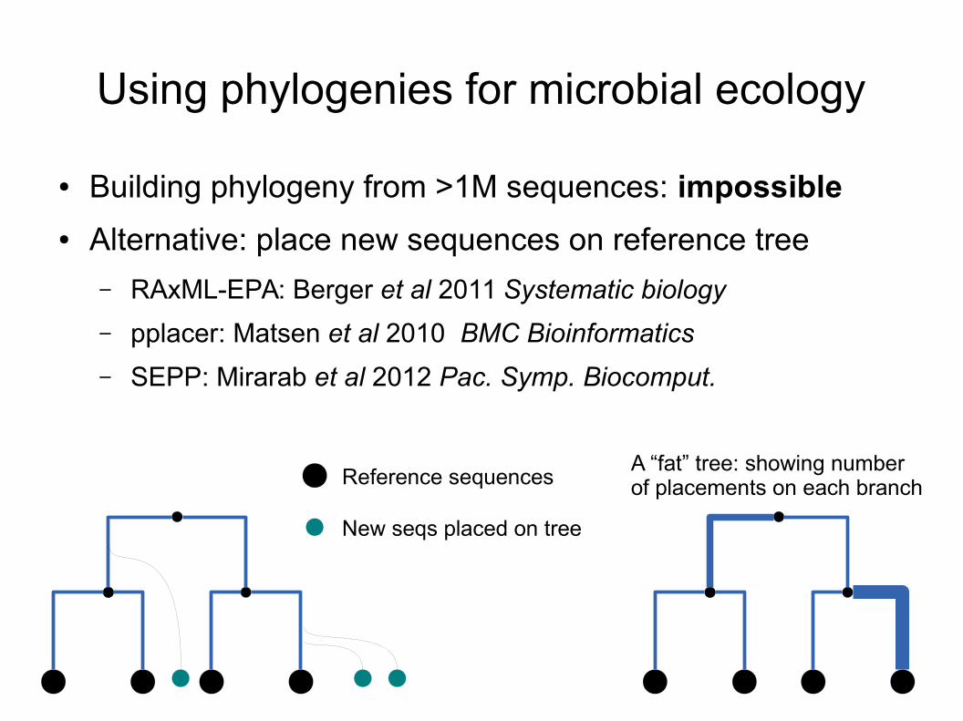
Using phylogenies for microbial ecology

● Building phylogeny from >1M sequences: impossible

● Alternative: place new sequences on reference tree

– RAxML-EPA: Berger et al 2011 Systematic biology

– pplacer: Matsen et al 2010 BMC Bioinformatics

– SEPP: Mirarab et al 2012 Pac. Symp. Biocomput.

Reference sequences

New seqs placed on tree

A “fat” tree: showing numberof placements on each branch

Handling uncertainty

● Bayesian placement (pplacer)

– Calculate probability of new sequence on each branch

– pplacer can do this quickly, analytically (no MCMC)

placement distributionviewed as a fat tree

A single sequence with uncertain placement

Placement is starting to look better than OTUs

Uncertainty in many sequences

● Combine placement distributions from all seqs in sample

+ =

Sequence 1 Sequence 2 Whole sample

Using a placement distrib.: alpha diversity

● Phylogenetic diversity is sum length of branches covered

● BWPD: Balance-weighted phylogenetic diversity (Barker 2002)

– Intuition: weight the contribution each lineage makes to PD by its relative abundance

– Weights can reflect placement uncertainty

} 0.01

Sample PD is 0.01 + 0.01 + 0.01 + 0.01 + 0.01 = 0.05

BWPDθ: partial weighting for PD

● A 1-parameter function interpolates between PD and BWPD (Matsen & McCoy 2013, PeerJ)

● When θ = 0 it is simply PD. θ = 1 it is BWPD.

● Matsen & McCoy compare:

– OTU-based diversity metrics

– Phylogenetic diversity (Faith 1992)

– Phylogenetic entropy (Rao 1982, Warwick & Clarke 1995)

– Phylogenetic quadratic entropy (Allen, Kon & Bar-Yam 2009)

– qD(T) (Chao, Chiu, Jost 2010)

– BWPD (Barker 2002)

– BWPDθ

on 3 different microbial communities, measuring correlation of diversity & phenotype

– Vaginal, oral, & skin microbiomes

● θ=0.25 & θ=0.5 have highest correlation with microbial community phenotypes

● OTU based diversity metrics have least correlation with phenotype

Beta diversity: Edge Principal Component Analysis

● Edge PCA for exploratory data analysis (Matsen and Evans 2013)

● Given E edges and S samples:

– For each edge, calculate difference in placement mass on either side of edge

– Results in E x S matrix

– Calculate E x E covariance matrix

– Calculate eigenvectors, eigenvalues of covariance matrix

● Eigenvector: each value indicates how “important” an edge is in explaining differences among the S samples

Example calculating a matrix entry for an edge:This edge gets 5-2=3

mass=5 mass=2

Edge PCA: visually

Branches are thickened & colored according to the amount they shift the sample along an axis

Matsen & Evans 2012 PLoS ONE

(full tree not shown)

Edge PCA and the vagina

● Samples colored according to Nugent score of bacterial vaginosis: blue → healthy, red → sick (Matsen & Evans 2012)

How to do it?

1. Find reference sequences

2. Align reference sequences

3. Infer reference phylogeny

4. For each sample:

4.1. Add sequences to alignment

4.2. Place sequences on tree

5. Alpha & Beta diversity analysis

Each step is a unix command

PhyloSift: genome and metagenome phylogeny

Illumina reads placed onto reference gene family trees● 40 “elite” families: universal among ~4000 Bact, Arch, Euk genomes (Lang et al 2013, Wu et al 2013)● 350,000 “extended” families: SFAMs (Sharpton et al 2012)● Amino-acid and nucleotide alignments+phylogenies

Treangen et al 2013.

Darling et al 2014 PeerJ.

Using phylosift

Download phylosift: phylosift.wordpress.org

bin/phylosift all --output=hmp tutorial_data/HMP_1.fastq.gz

open hmp/HMP_1.fastq.gz.html

bin/guppy fpd --theta 0.25,0.5 hmp/*.gz.jplace

bin/guppy epca --prefix pca hmp/*.gz.jplace

More examples at: phylosift.wordpress.org

Raw illumina data

Shows taxonomic plot (Mac)

Alpha diversity

Beta diversity (min 3 samples)

QIIME vs. PhyloSift

Data from Yatsunenko et al 2012. 16S amplicon & metagenomes from same samples

Phylosift on proteins &16S produces similarresults to QIIME onamplicon data

Phylogenetic alpha diversity

Data from Yatsunenko et al 2012

● Growth in PD over life

● BWPD is biphasic

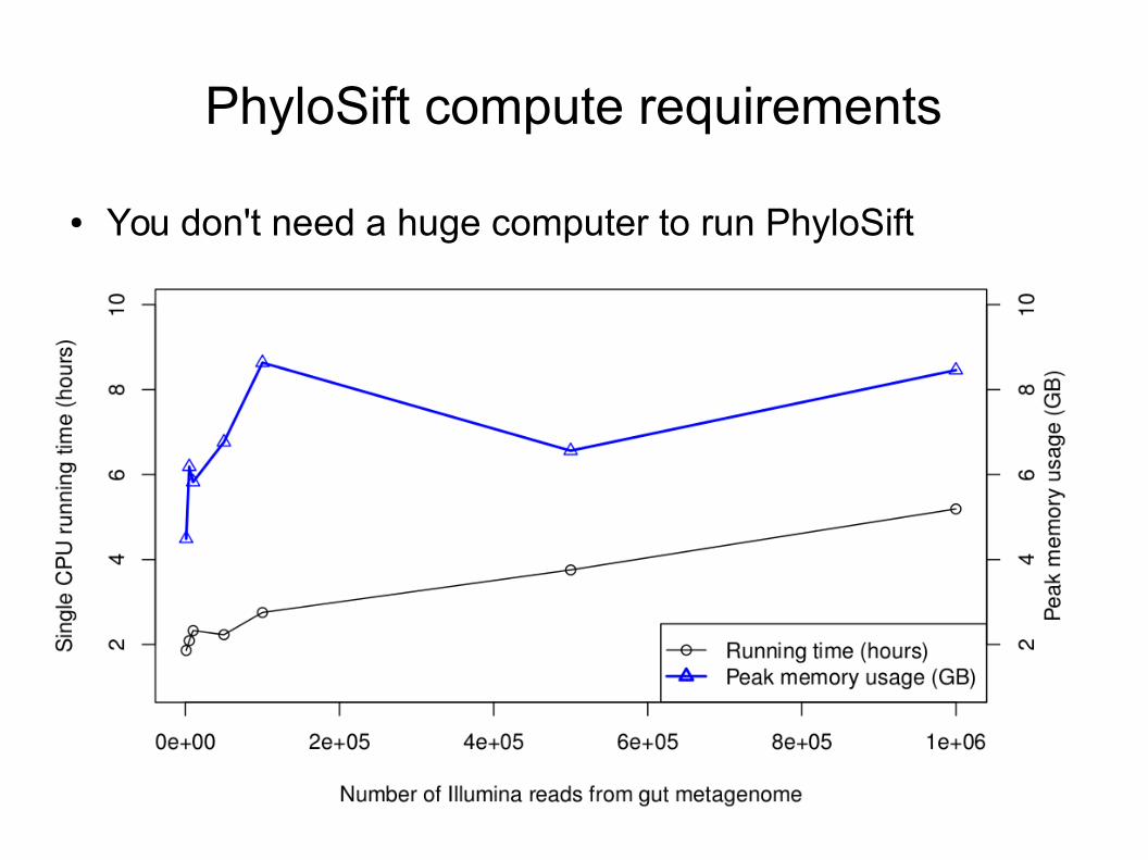
PhyloSift compute requirements

● You don't need a huge computer to run PhyloSift

phylosift and major life events

On December 3rd 2010, Kai and his microbiome were born

Lots of nappies, lots of sampling

March 1st 2011: a lot of poop in tubes and no idea how to get it through USA quarantine

Tiffanie Nelson at UNSW:Extracted DNA with PowerSoil kits, mailed to USA

Kai Darling born 3rd Dec. 2010 in California, flew to Sydney 3.5 weeks later

Metagenomics on a shoestring budget*

“Homebrew” Illumina Nextera library prep protocol:

Goal: metagenomics as easy as 16S amplicon studies

Strategy: Transposon-catalyzed library prep. Express & purify Tn5 from pWH1891. Custom adapters. 2.5ng inputPool samples as early as possible.

Results: Sequenced 45 time points in HiSeq 2000 lane~ $1 / library reagent costs, 100s of libraries in a day, NO ROBOTS

*Infant microbiome sequencing sponsored by private funds

PhyloSift view of fecal microbiome at three weeks age

● Tree-browsing of read placement mass (via archaeopteryx)

● Taxonomic summary plots in Krona (Ondov et al 2011)

Alpha diversity of gut communities vs. time

● Standard & balance-weighted PD (McCoy & Matsen, 2013)

● Phylogenetic diversity (PD) decreases?!

Pearson's cor: -0.44, p = 0.005(p < 10-6 without formula samples)

Pearson's cor: 0.21, p = 0.18 (p = 0.0071 w/o formula)

B. thetaiotaomicron becomes dominant

Formula-fed days (red)

Phylogenetic “Edge PCA” on infant fecal microbiome

Up: Bacteroides, Down: Bifidobacterium

Up:

Bifi

doba

cter

ium

long

um

3rd PC (1%):StaphylococcusVeillonella

Edge PCA: explain variation in community structure among many samplesMatsen & Evans 2013 PLoS ONE

Chan et al In prep

Formula-fed samples within one day

One week on formula,

Six poops in one day.

Up: Bacteroides, Down: Bifidobacterium

Up:

Bifi

doba

cter

ium

long

um

Chan et al In prep

Thanks!