computational geomechanics: simulations of static...
TRANSCRIPT

Computational Geomechanics:Simulations of Static and Dynamic
Behavior of Foundation System
Boris JeremicDepartment of Civil and Environmental Engineering
University of California, Davis
OpenSees User Workshop
August 21-22, 2003 , Richmond Field Station
Supported in part by the NSF, PEER, Caltrans, and Cal–EPA.
Collaborators: Professors Zhaohui Yang (UAA), Sashi Kunnath (UCD), Gregory Fenves (UCB),
Jacobo Bielak (CMU), Zhaojun Bai (UCD), George Karypis (UMN), Drs. Francis McKenna
(UCB), and graduate students Xiaoyan Wu (UCD) Ritu Jain (UCD), Qing Liu (UCD), Jinxiu
Liao (UCD). Guanzhou Jie (UCD).
Jeremic, OpenSees Workshop, Aug. 2003 1

Motivation
• Create high fidelity models of constructed facilities (bridges, build-
ings, port structures, dams...).
• Models will live concurrently with the physical system they repre-
sent.
• Models to provide owners and operators with the capabilities to
assess operations and future performance.
• Use observed performance to update and validate models through
simulations.
Jeremic, OpenSees Workshop, Aug. 2003 2
Goal
• Develop and use Computational tools based on
• Geomechanics to
• Investigate behavior of solids and structures made of geomaterials
Jeremic, OpenSees Workshop, Aug. 2003 3

Overview
• Enabling Technologies (ET)
– Template Elasto–Plasticity– Full Coupling of Solid and Fluid– Domain Reduction Method– Distributed Memory Parallel Computing
• Geomechanics Applications (GA)
– Constitutive behavior of test specimens– Behavior of piles in layered soils– Interactions of piles in pile groups– Wave propagation in saturated soils– Seismic behavior of soils and soil-structure interactions
• Currently in Works (CW)
– General Large Deformations– Distributed Parallel Computing
Jeremic, OpenSees Workshop, Aug. 2003 4

ET: Template Elasto–Plasticity
Yield function (or lack of YF), potential function (and/or flow
directions), hardening/softening laws (scalar, rotational/translational
kinematic, distortional...)
• Independent definitions of:
1. Yield function (and it’s derivatives)
2. Plastic flow direction (first and second derivatives of potential
function)
3. Evolutions laws for the above two
• This is used to create Template Elastic–Plastic Models
Jeremic, OpenSees Workshop, Aug. 2003 5

ET: Template Elastic–PlasticModels
• von Mises
• Drucker–Prager
• Rounded Mohr–Coulomb
• Cam–Clay
• Mazari–Dafalias (bounding surface plasticity)
• Parabolic Leon
• User added
• Any combination of the above using isotropic or kinematic hard-
ening
• Hierarchical database of models (by materials)
Jeremic, OpenSees Workshop, Aug. 2003 6

ET: Template Examples
0 2 4 6 8 100
5
10
15
20
25
30
35
40
εa (%)
q (k
Pa)
0 2 4 6 8 10−7
−6
−5
−4
−3
−2
−1
0
1
εa (%)
ε v (%
)
0 2 4 6 8 100
5
10
15
20
25
30
εa (%)
q (k
Pa)
0 2 4 6 8 100
0.1
0.2
0.3
0.4
0.5
εa (%)
ε v (%
)
0 2 4 6 8 100
5
10
15
20
25
30
εa (%)
q (k
Pa)
0 2 4 6 8 100
0.5
1
1.5
2
2.5
3
3.5
εa (%)
ε v (%
)
0 2 4 6 8 100
5
10
15
20
25
30
35
40
εa (%)
q (k
Pa)
0 2 4 6 8 10−1
−0.5
0
0.5
εa (%)
ε v (%
)
0 2 4 6 8 100
50
100
150
200
εa (%)
q (k
Pa)
0 2 4 6 8 100
0.5
1
1.5
2
2.5
3
εa (%)
ε v (%
)
0 5 10 150
10
20
30
40
50
60
εa (%)
q (k
Pa)
0 5 10 15−12
−10
−8
−6
−4
−2
0
2
εa (%)
ε v (%
)
Jeremic, OpenSees Workshop, Aug. 2003 7

ET: Template Cyclic Examples
−0.4 −0.2 0 0.2 0.4−10
−5
0
5
10
15
εa (%)
q (k
Pa)
−0.4 −0.2 0 0.2 0.40
0.1
0.2
0.3
0.4
0.5
0.6
0.7
εa (%)
ε v (%
)
−0.4 −0.2 0 0.2 0.4−10
−5
0
5
10
εa (%)
q (k
Pa)
−0.4 −0.2 0 0.2 0.4−0.15
−0.1
−0.05
0
0.05
0.1
0.15
0.2
0.25
εa (%)
ε v (%
)
−0.15 −0.1 −0.05 0 0.05 0.1 0.15−20
−10
0
10
20
30
εa (%)
q (k
Pa)
−0.1 −0.05 0 0.05 0.1 0.15−0.5
0
0.5
1
1.5
2
2.5
3
εa (%)
ε v (%
)
Jeremic, OpenSees Workshop, Aug. 2003 8

ET: Full Coupling of Solid and Fluid
General form (Zienkiewicz et al.), full coupling, (currently only small
deformations)
DOFs: uLj → solid displacement pL → fluid pressure ULj → fluid
displacement
(Ms)KijL 0 0
0 0 0
0 0 (Mf)KijL
¨uLj
¨pL¨ULj
+
(C1)KijL 0 −(C2)KijL0 0 0
−(C2)LjiK 0 (C3)KijL
˙uLj
˙pL˙ULj
+
(KEP )KijL −(G1)KiL 0
−(G1)LjK −(P )KL −(G2)LjK0 −(G2)KiL 0
uLjpLULj
=
(fs)Ki0
(ff)Ki
(C1)KijL = (C2)KijL = (C3)KijL =
∫Ω
Nu,UK n
2k−1ij N
u,UL dΩ
Jeremic, OpenSees Workshop, Aug. 2003 9

ET: Domain Reduction Method
• Based on work by Bielak et al. at CMU.
• Superposition of the large scale domain + local geologic feature
• Seismic motions and accelerations input at the layer of elements
that encompass an elastic–plastic zone (using SHAKE, Green’s
functions, Quake, SCEC...)
• Non–reflecting boundaries
Fault
Plastic (Soil) "Bowls"
Jeremic, OpenSees Workshop, Aug. 2003 10

Geomechanics Applications
Constitutive behavior of test specimens
Behavior of piles in layered soils
Interactions of piles in pile groups
Wave propagation in saturated soils
Seismic behavior of soils and soil-structure interactions
Jeremic, OpenSees Workshop, Aug. 2003 11
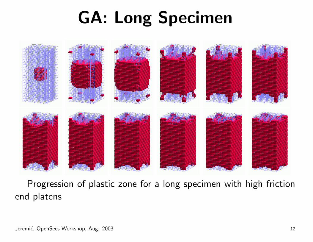
GA: Long Specimen
Progression of plastic zone for a long specimen with high friction
end platens
Jeremic, OpenSees Workshop, Aug. 2003 12

GA: Non–Level End Platens
Jeremic, OpenSees Workshop, Aug. 2003 13

GA: Constitutive Response?
0 0.5 1 1.5 2 2.5 30
50
100
150
200
250
300
350
Shear Strain ε (%)
q (k
Pa)
Without Friction − Cubic Sample With Friction − Cubic SampleWithout Friction − 2 to 1 Sample With Friction − 2 to 1 Sample
Jeremic, OpenSees Workshop, Aug. 2003 14

GA: Constitutive Response?
0 0.5 1 1.5 2 2.5 3 3.534
34.5
35
35.5
36
36.5
37
37.5
38
Max. inclination angle (deg)
Mob
ilize
d fr
ition
ang
le a
t 2.0
% a
xial
str
ain
Actual friction angle: 37.0o
Jeremic, OpenSees Workshop, Aug. 2003 15

GA: Single Pile in Layered Soils
−1000 0 1000 2000−10
−8
−6
−4
−2
0
2
SAND
φ = 37.1o
−1.718
SOFT CLAY
Cu = 21.7 kPa
−3.436
SAND
φ = 37.1o
Bending Moment (kN.m)
Dep
th (
m)
SAND
φ = 37.1o
−1.718
SOFT CLAY
Cu = 21.7 kPa
−3.436
SAND
φ = 37.1o
SAND
φ = 37.1o
−1.718
SOFT CLAY
Cu = 21.7 kPa
−3.436
SAND
φ = 37.1o
−400 −200 0 200 400 600−10
−8
−6
−4
−2
0
2
Shear Force (kN)−100 0 100 200 300
−10
−8
−6
−4
−2
0
2
Lateral Resistance (kN/m)−1000 0 1000 2000
−10
−8
−6
−4
−2
0
2
SAND
φ = 37.1o
−1.718
SOFT CLAY
Cu = 21.7 kPa
−3.436
SAND
φ = 37.1o
Bending Moment (kN.m)
Dep
th (
m)
−400 −200 0 200 400 600−10
−8
−6
−4
−2
0
2
Shear Force (kN)−100 0 100 200 300
−10
−8
−6
−4
−2
0
2
Lateral Resistance (kN/m)
Jeremic, OpenSees Workshop, Aug. 2003 16

GA: p− y Response for Single Pilein Layered Soils
0 2 4 6 8 10 120
50
100
150
200
250
300
Lateral Displacement y (cm)
Late
ral P
ress
ure
p (k
N/m
)
Depth −0.322Depth −0.537Depth −0.752Depth −0.966Depth −1.181Depth −1.396Depth −1.611Depth −1.825Depth −2.040Depth −2.255Depth −2.470Depth −2.684
0 2 4 6 8 10 120
50
100
150
200
250
300
Lateral Displacement y (cm)La
tera
l Pre
ssur
e p
(kN
/m)
Depth −0.322Depth −0.537Depth −0.752Depth −0.966Depth −1.181Depth −1.396Depth −1.611Depth −1.825Depth −2.040Depth −2.255Depth −2.470Depth −2.684
• Influence of soft layers propagates to stiff layers and vice versa
• Can have significant effects in soils with many layers
Jeremic, OpenSees Workshop, Aug. 2003 17
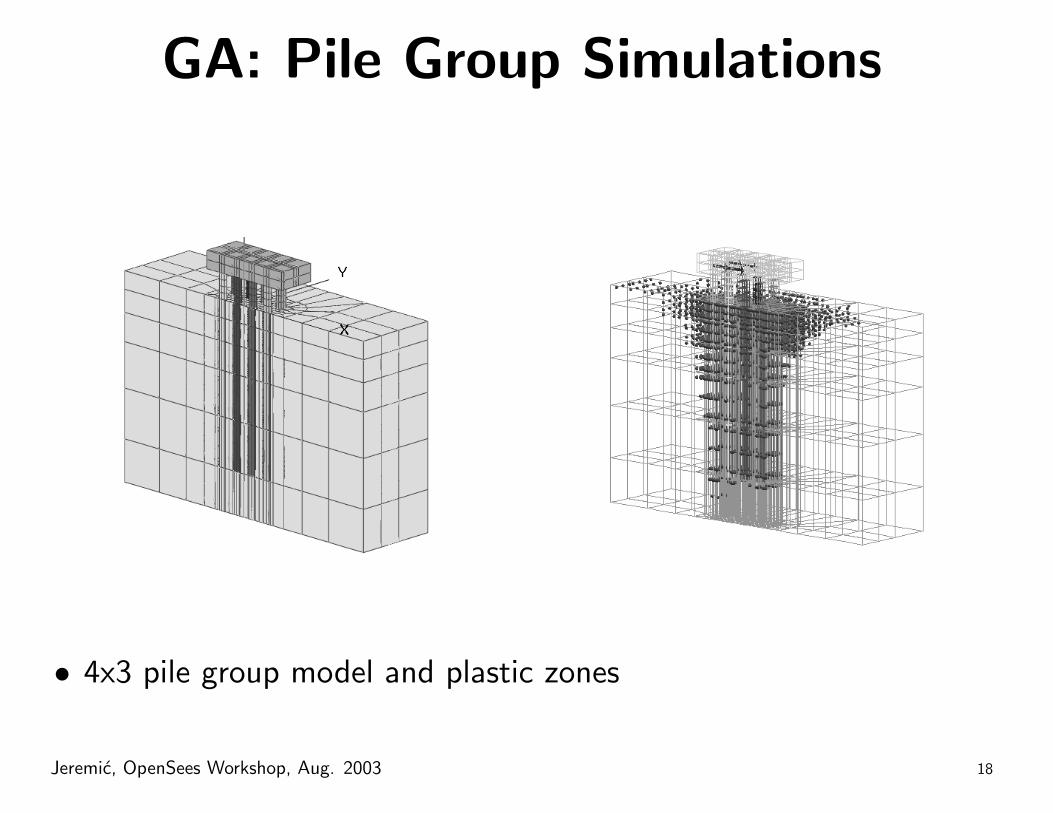
GA: Pile Group Simulations
• 4x3 pile group model and plastic zones
Jeremic, OpenSees Workshop, Aug. 2003 18

GA: Out of Plane Effects
• Out-of-loading-plane bending moment diagram,
• Out-of-loading-plane deformation.
Jeremic, OpenSees Workshop, Aug. 2003 19

GA: Load Distribution per Pile
0 1 2 3 4 5 6 7 8 9 10 115
6
7
8
9
10
11
12
13
14
15La
tera
l Loa
d D
istr
ibut
ion
in E
ach
Pile
(%
)
Displacement at Pile Group Cap (cm)
Trail Row, Side PileThird Row, Side PileSecond Row, Side PileLead Row, Side PileTrail Row, Middle PileThird Row, Middle PileSecond Row, Middle PileLead Row, Middle Pile
Jeremic, OpenSees Workshop, Aug. 2003 20

GA: Piles Interaction at -2.0m
• Note the difference in response curves (cannot scale single pile
response for multiple piles)
Jeremic, OpenSees Workshop, Aug. 2003 21
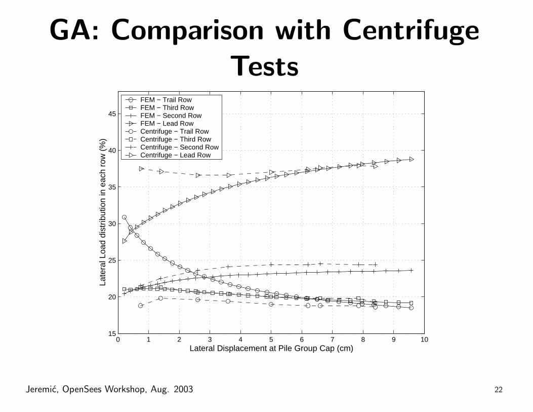
GA: Comparison with CentrifugeTests
0 1 2 3 4 5 6 7 8 9 1015
20
25
30
35
40
45
Late
ral L
oad
dist
ribut
ion
in e
ach
row
(%
)
Lateral Displacement at Pile Group Cap (cm)
FEM − Trail RowFEM − Third RowFEM − Second RowFEM − Lead RowCentrifuge − Trail RowCentrifuge − Third RowCentrifuge − Second RowCentrifuge − Lead Row
Jeremic, OpenSees Workshop, Aug. 2003 22

GA: Layering Effects (S–C–S)
0.5 0.6 0.7 0.8 0.9 1 1.10
0.5
1
1.5
2
2.5
3
3.5
4
4.5
5
Dis
tanc
e fr
om L
ayer
Inte
rfac
e (x
D)
Lateral Pressure Ratio Psand clay
/ Psand
Sand:φ = 37o, Clay:Su = 15kPaSand:φ = 37o, Clay:Su = 25kPaSand:φ = 37o, Clay:Su = 35kPa
Strength reduction (layering effects) extending to 4xD (in thiscase)
Jeremic, OpenSees Workshop, Aug. 2003 23

GA: Seismic Wave PropagationModel
0 0.5 1 1.5 2 2.5 3 3.5 4 4.5 5
−27.3
−23.3
−21.8
−18.3
−14.8
−11.8
−8.8
−6.3
−3.3
−1.8
0.0
Time (s)
Acc
eler
atio
n (m
/s2 )
0 0.5 1 1.5 2 2.5 3 3.5 4 4.5 5−27.3
−23.3
−21.8
−18.3
−14.8
−11.8
−8.8
−6.3
−3.3
−1.8
0.0
Time (s)
Dis
plac
emen
t (m
)
Jeremic, OpenSees Workshop, Aug. 2003 24

GA: Seismic Wave PropagationSoft Soil
0 0.5 1 1.5 2 2.5 3 3.5 4 4.5 5
0.0625−27.3
0.0633−23.3
0.0678−21.8
0.0749−18.3
0.0846−14.8
0.0960−11.8
0.1076 −8.8
0.1160 −6.3
0.1208 −3.3
0.1207 −1.8
0.1181 0.0
Max
Time (s)
Dis
plac
emen
t (m
)
Z
0 0.5 1 1.5 2 2.5 3 3.5 4 4.5 5
0.0622−25.0
0.0779−21.0
0.0837−19.5
0.0982−15.0
0.1069−11.0
0.1123 −7.0
0.1169 −4.3
0.1174 −3.6
0.1179 −1.8
0.1181 0.0
0.1183 1.8
0.1178 3.6
0.1173 4.3
0.1129 7.0
0.1075 11.0
0.0984 15.0
0.0837 19.5
0.0779 21.0
0.0622 25.0
Max
Time (s)
Dis
pala
cem
ent (
m)
Y
Jeremic, OpenSees Workshop, Aug. 2003 25
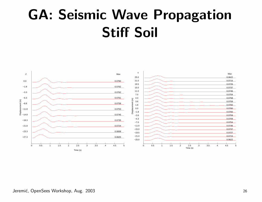
GA: Seismic Wave PropagationStiff Soil
0 0.5 1 1.5 2 2.5 3 3.5 4 4.5 5
0.0625−27.3
0.0658−23.3
0.0724−21.8
0.0735−18.3
0.0745−14.8
0.0753−11.8
0.0758 −8.8
0.0761 −6.3
0.0762 −3.3
0.0762 −1.8
0.0760 0.0
Max
Time (s)
Dis
plac
emen
t (m
)
Z
0 0.5 1 1.5 2 2.5 3 3.5 4 4.5 5
0.0622−25.0
0.0715−21.0
0.0727−19.5
0.0737−15.0
0.0746−11.0
0.0754 −7.0
0.0759 −4.3
0.0759 −3.6
0.0760 −1.8
0.0760 0.0
0.0760 1.8
0.0759 3.6
0.0758 4.3
0.0754 7.0
0.0746 11.0
0.0737 15.0
0.0726 19.5
0.0715 21.0
0.0622 25.0
Max
Time (s)
Dis
plac
emen
t (m
)
Y
Jeremic, OpenSees Workshop, Aug. 2003 26

GA: SSI Model
0 0.5 1 1.5 2 2.5 3 3.5 4 4.5 5
−38.0
−30.0−28.0
−20.0
−16.0
−12.0
−8.0
−4.0
0.0
Time (s)
Acc
eler
atio
n (m
/s2 )
0 0.5 1 1.5 2 2.5 3 3.5 4 4.5 5−38.0−30.0
−28.0
−20.0
−16.0
−12.0
−8.0
−4.0
0.0
Time (s)
Dis
plac
emen
t (m
)
Jeremic, OpenSees Workshop, Aug. 2003 27

GA: SSI Model Free FieldStiff Elastic–Plastic Soil
0 1 2 3 4 5 6 7 8 9 10
0.0000−38.0
0.0052−30.00.1055−28.0
0.1142−20.0
0.1183−16.0
0.1219−12.0
0.1576 −8.0
0.1947 −4.0
0.2002 0.0
Time (s)
Dis
plac
emen
t (m
)
Z(m) Max
0 1 2 3 4 5 6 7 8 9 10
0.2002 0.0
0.1937 4.0
0.1749 8.0
0.1261 12.0
0.1231 16.0
0.1139 24.0
0.0124 26.0
0.0000 34.0
Time (s)
Dis
plac
emen
t (m
)
Z(m) Max
Jeremic, OpenSees Workshop, Aug. 2003 28
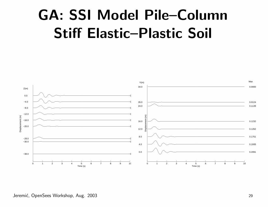
GA: SSI Model Pile–ColumnStiff Elastic–Plastic Soil
0 1 2 3 4 5 6 7 8 9 10
0.0000−38.0
0.0052−30.00.1055−28.0
0.1142−20.0
0.1183−16.0
0.1222−12.0
0.1496 −8.0
0.1899 −4.0
0.2091 0.0
Time (s)
Dis
plac
emen
t (m
)
Z(m) Max
0 1 2 3 4 5 6 7 8 9 10
0.2091 0.0
0.1935 4.0
0.1751 8.0
0.1262 12.0
0.1232 16.0
0.1139 24.0
0.0124 26.0
0.0000 34.0
Time (s)
Dis
plac
emen
t (m
)
Y(m) Max
Jeremic, OpenSees Workshop, Aug. 2003 29
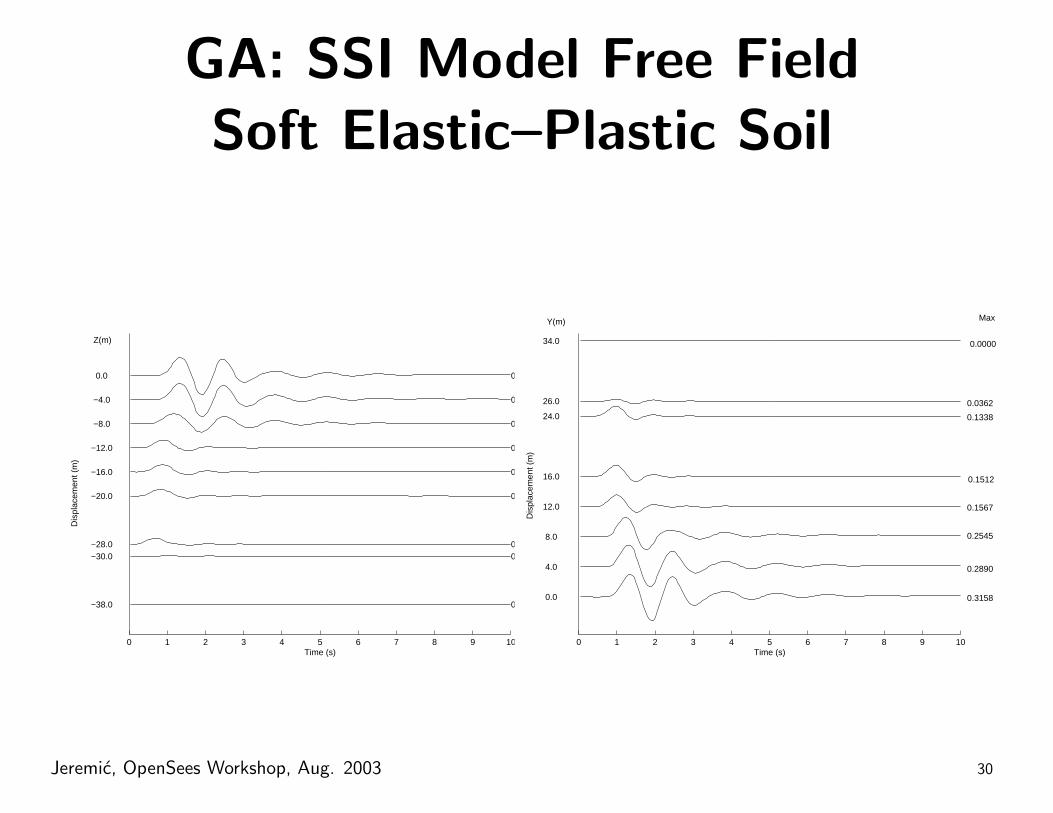
GA: SSI Model Free FieldSoft Elastic–Plastic Soil
0 1 2 3 4 5 6 7 8 9 10
0.0000−38.0
0.0140−30.00.0971−28.0
0.1096−20.0
0.1190−16.0
0.1261−12.0
0.1622 −8.0
0.2823 −4.0
0.3158 0.0
Time (s)
Dis
plac
emen
t (m
)
Z(m)
0 1 2 3 4 5 6 7 8 9 10
0.3158 0.0
0.2890 4.0
0.2545 8.0
0.1567 12.0
0.1512 16.0
0.1338 24.0
0.0362 26.0
0.0000 34.0
Time (s)
Dis
plac
emen
t (m
)
Y(m) Max
Jeremic, OpenSees Workshop, Aug. 2003 30

GA: SSI Model Pile–ColumnSoft Elastic–Plastic Soil
0 1 2 3 4 5 6 7 8 9 10
0.0000−38.0
0.0140−30.00.0976−28.0
0.1094−20.0
0.1207−16.0
0.1227−12.0
0.1328 −8.0
0.2448 −4.0
0.3680 0.0
Time (s)
Dis
plac
emen
t (m
)
Z(m) Max
0 1 2 3 4 5 6 7 8 9 10
0.3680 0.0
0.2896 4.0
0.2536
8.0
0.1549
12.0
0.1497
16.0
0.1331
24.0 0.0356
26.0
0.0000 34.0
Time (s)
Jeremic, OpenSees Workshop, Aug. 2003 31

SSI Model: Pile–Column Behavior
0 1 2 3 4 5 6 7 8 9 10−0.03
−0.02
−0.01
0
0.01
0.02
0.03
0.04
Dis
plac
emnt
(m
)
Time (s)0 1 2 3 4 5 6 7 8 9 10
−0.25
−0.2
−0.15
−0.1
−0.05
0
0.05
0.1
0.15
0.2
0.25
Dis
plac
emen
t (m
)
Time (s)
Stiff soil Soft soil
Jeremic, OpenSees Workshop, Aug. 2003 32

SSI Model: Preliminary SeismicResults
0 5 10 15 20 25 30 35 40
0.0000−38.0
0.0077−30.0
0.0783−28.0
0.0791−20.0
0.0844−16.0
0.0878−12.0
0.1248 −8.0
0.1800 −4.0
0.1946 0.0
Time (s)
Dis
plac
emen
t (m
)
Z(m) Max
0 5 10 15 20 25 30 35 40
0.0000−38.0
0.0224−30.0
0.0879−28.0
0.1102−20.0
0.1161−16.0
0.1227−12.0
0.3961 −8.0
0.6258 −4.0
0.6928 0.0
Time (s)
Dis
plac
emen
t (m
)
Z(m) Max
Stiff soil Soft soil
Jeremic, OpenSees Workshop, Aug. 2003 33

GA: Wave Propagation inSaturated Soils
0 0.05 0.1 0.15 0.2 0.25 0.3−4
−3
−2
−1
0
1
2x 10
−3
Sol
id D
ispl
acem
ent (
m)
Top node2m from top4m from top6m from top
0 0.05 0.1 0.15 0.2 0.25 0.3−0.5
0
0.5
1
Por
e pr
essu
re (
kPa)
0 0.05 0.1 0.15 0.2 0.25 0.3−4
−3
−2
−1
0
1
2x 10
−3
Time (sec)
Flu
id D
ispl
acem
ent (
m)
0 0.05 0.1 0.15 0.2 0.25 0.3−4
−3
−2
−1
0
1
2x 10
−3
Sol
id D
ispl
acem
ent (
m)
Top node2m from top4m from top6m from top
0 0.05 0.1 0.15 0.2 0.25 0.3−0.5
0
0.5
1
Por
e pr
essu
re (
kPa)
0 0.05 0.1 0.15 0.2 0.25 0.3−4
−3
−2
−1
0
1
2x 10
−3
Time (sec)
Flu
id D
ispl
acem
ent (
m)
Half space, ramp load k = 10−3,5m/s
Jeremic, OpenSees Workshop, Aug. 2003 34

GA: Soil–Structure Interaction
Jeremic, OpenSees Workshop, Aug. 2003 35

GA: SSI AdvantageousH
oriz
anta
l Dis
plac
emen
t (m
)
0.1
0.05
0
−0.05
−0.1
−0.150 5 10 15 20 25 30 35 40 45 50
Time (Sec)
Fixed Model SFSI Model
She
ar F
orce
(N
)
4
6
2
0
−2
−4
−6
−8
x 10
Fixed ModelSFSI model
−0.15 −0.1 −0.05 0Displacement (m)
0.05 0.1
6
Kobe–JMA
Jeremic, OpenSees Workshop, Aug. 2003 36

GA: SSI DisadvantageousH
oriz
anta
l Dis
plac
emen
t (m
)
Time (Sec)0 5 10 15 20 25 30 35 40
Fixed Model SFSI Model
0.5
0.4
0.3
0.2
0.1
0
−0.1
−0.2
−0.3
−0.4
−0.5
6
She
ar F
orce
(N
)
−2
0
2
4
6
−4
−6
−8−0.5 −0.4 −0.3 −0.2 −0.1 0 0.1 0.2 0.3 0.4 0.5
Displacement (m)
Fixed ModelSFSI model
x 10
LP–Corralitos
Jeremic, OpenSees Workshop, Aug. 2003 37

Currently in Works
General Large Deformations
Distributed Parallel Computing
Jeremic, OpenSees Workshop, Aug. 2003 38

CW: General Large Deformations
• LD (Eij = 12 (ui,j + uj,i + ui,juj,i)) vs. SD (εij = 1
2(ui,j + uj,i)• Multiplicative decomposition of (Fij = xi,j = F eki F
pkj)
• MacLaurin series expansion of the exponent of flow direction, for
general anisotropic material and cyclic loading• Stress measures (first and second Piola–Kirchhoff, Mandel, Kirch-
hoff, Cauchy)
ijε
Eij
500%
1000%
1500%
2000%
2500%
0.0 1.0 2.0 3.0 4.0 5.0 6.0
Errorshea
r st
rain
deformation (arctan )Φ
Φ
Fp
Fe Fe
-1
Reference
Configuration
X
d X
Ω0Intermediate
Configurationdx
Ω
dx
Current
Configuration
x
Ω
σ x
F
X ux
Jeremic, OpenSees Workshop, Aug. 2003 39

CW: Distributed MemoryParallel Computing
• Distributed memory parallel (DMP) computational model.
• Portable from Beowulf clusters (local networks, bootable CDs) to
commercial parallel machines.
Jeremic, OpenSees Workshop, Aug. 2003 40

Pre– and Post–Processing
• Many small packages around, available for UNIX–like and/or MS
Windows systems (Mac?).
• Work on pre and post processing packages that are problem specific
Jeremic, OpenSees Workshop, Aug. 2003 41

Joey3D
Jeremic, OpenSees Workshop, Aug. 2003 42
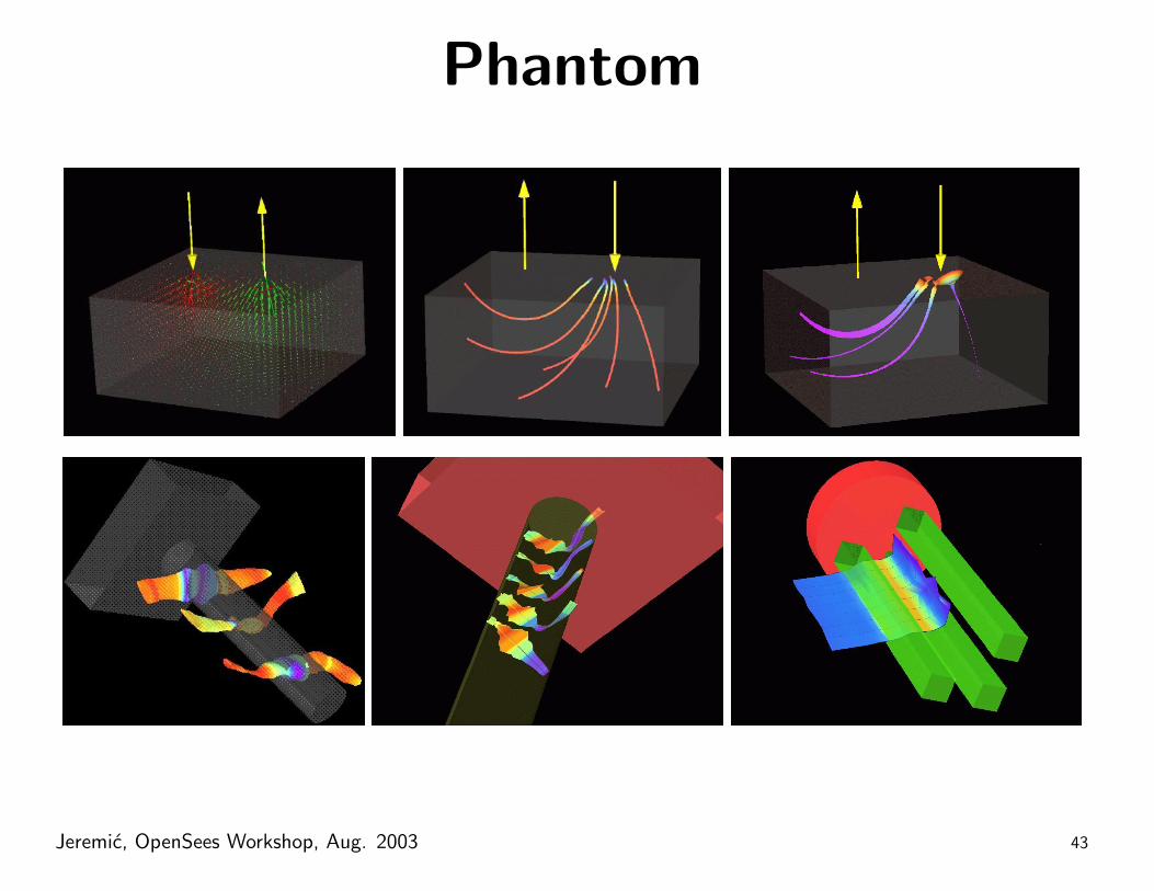
Phantom
Jeremic, OpenSees Workshop, Aug. 2003 43

Conclusions
• Examples, lecture notes, executables available at:
http://sokocalo.engr.ucdavis.edu/ jeremicand at
http://opensees.berkeley.edu/
• Manual is constantly being improved
• Executables available for both UNIX-like (up–to–date, preferable)
and MS Windows.
• MS Windows, soon to have up to date executables
Jeremic, OpenSees Workshop, Aug. 2003 44