ARTICLE IN PRESS

Chemical Engineering Science 65 (2010) 753–771

Contents lists available at ScienceDirect

Chemical Engineering Science

0009-25

doi:10.1

� Corr

E-m

journal homepage: www.elsevier.com/locate/ces

Computational design of thermoset nanocomposite coatings: Methodologicalstudy on coating development and testing

Jie Xiao, Yinlun Huang �, Charles Manke

Department of Chemical Engineering and Materials Science, Wayne State University, Detroit, MI 48202, USA

a r t i c l e i n f o

Article history:

Received 21 March 2009

Received in revised form

8 July 2009

Accepted 11 September 2009Available online 17 September 2009

Keywords:

Thermoset nanocomposites

Nanocoating

Computational design

Off-lattice Monte Carlo simulation

Microstructure

Curing

09/$ - see front matter & 2009 Elsevier Ltd. A

016/j.ces.2009.09.028

esponding author. Tel.: +1313 577 3771; fax:

ail address: yhuang@wayne.edu (Y. Huang).

a b s t r a c t

Thermoset nanocomposites (TSNCs) may offer significantly improved performance over conventional

thermoset materials, and thus are attractive for wide industrial applications, especially in the coating

industry. Design of TSNCs via experiment, however, faces various technical challenges due to design

complexity. Computational design can provide deep insights and identify superior design solutions

through exploring opportunities in a usually huge design space. This paper introduces a generic

computational methodology for the design, characterization, and testing of TSNC-based coatings. A

distinct feature of the methodology is its capability of generating quantitative correlations among

material formulation, processing condition, coating microstructure and property, coating performance,

and processing efficiency. The correlations can enable a comprehensive analysis for optimal TSNC

coating design. Case studies will demonstrate the methodological efficacy and attractiveness.

& 2009 Elsevier Ltd. All rights reserved.

1. Introduction

Development of thermoset nanocomposites (TSNCs) for coat-ing applications has drawn increasing attention over recent years.This type of nanocomposites is usually designed by adding a smallamount of organo-modified inorganic nanoparticles into a con-ventional thermoset resin. The resulting material is then appliedto a substrate and cured at an elevated temperature to form acoating layer. TSNCs, when compared with conventional thermo-set polymers, are capable of substantially improving coatingperformance, in terms of coating’s mechanical, barrier and flame-retardant properties, and even possessing new functionalities, e.g.,self-cleaning and self-healing. It is believed that TSNCs will havewide industrial applications (Kotsikova, 2007).

In TSNC development, a deep understanding of the dependenceof coating properties on material composition is essential. Variousexperimental efforts have been made to reveal the dependence.Nobel et al. (2007) developed a number of waterborne nanocom-posite resins for automotive coating applications. It was foundthat an incorporation of needle-shaped Boehmite, disc-shapedLaponite, or plate-shaped Montmorillonite into an aqueous acrylicresin could increase dramatically the stiffness of the cured filmand make the rheology of the binder more adjustable. Jalili et al.(2007) investigated a number of nanocomposite polyurethanecoatings. It was shown that adding 4–8 wt% of hydrophobic

ll rights reserved.

+1313 577 3810.

nano-silica to a two-pack acrylic polyol polyurethane clearcoatcould enhance the coating’s morphological, rheological, mechan-ical, and optical properties. Hosseinpour et al. (2005) showed thatan acrylic-melamine resin filled with spherical, polar-surface-treated alumina particles could improve greatly the mechanicalperformance of the coating.

The existing studies have improved the understanding on TSNCmaterials and their correlation to the properties of the nanos-tructured coatings. However, due to the existence of a largenumber of adjustable material parameters, the identification of anoptimal formulation solely through experiments is extremelychallenging. It must be pointed out that computational materialdesign can provide us with impressive freedom and control overthe investigated material parameters and product propertiesthrough allowing virtually any number of in silico experiments.Moreover, computational modeling and simulation should greatlyfacilitate identification of vast correlations among material,microstructure, property, and performance. Nevertheless, therehas been no such a computational methodology available forinvestigating TSNCs.

The known computational studies on polymer nanocompositematerials are nearly all for thermoplastic nanocomposites (TPNCs)(see Zeng et al., 2008). Molecular dynamics (MD) simulation (Starret al., 2002; Bedrov et al., 2003) and lattice and off-lattice MonteCarlo (MC) simulations (Vacatello, 2001, 2002; Zhang and Archer,2004; Ozmusul et al., 2005; Dionne et al., 2006) are among thetechniques used to investigate polymer chain conformation,nanoscale interactions, and material structural evolution andproperties. Investigation of TSNCs is much more challenging. First,

ARTICLE IN PRESS

J. Xiao et al. / Chemical Engineering Science 65 (2010) 753–771754

the polymeric material structural complexity in terms of themolecular weight distribution and the functional group distribu-tion must be taken into account. Second, multiple inter-correlatedchemical and physical phenomena occurred during the coatingformation process have to be properly characterized. Note that athermoset material must undergo a crosslinking reaction processin coating formation, but this is not the case for a thermoplasticmaterial application.

Most of the computational studies on structure–propertycorrelations for polymer nanocomposites are focused on model-based mechanical property quantification. The continuum-basedmicromechanics methods (e.g., Eshelby, Halphin-Tsai, and finiteelement based) and the non-continuum-based nanomechanicsmethods (e.g., MC, MD, and molecular mechanics based) are thetwo major types of techniques (Valavala and Odegard, 2005).Recently, multiscale methods received a great deal of attention(Sheng et al., 2004; Zeng et al., 2008), since they can characterizeappropriately the hierarchical morphology of polymer nanocom-posites, which is essential for accurate prediction of materialproperties. It has been noted by experimentalists that the detailedknowledge of the structure of crosslinked polymer networkmatrix is essential for developing structure–property relation-ships in TSNC systems (Bharadwaj et al., 2002; Nobel et al., 2007;Pluart et al., 2005). However, the known computational methodsare insufficient in studying TSNCs, because they either addressthermoplastic polymer matrix only or neglect detailed informa-tion about the microstructure of polymer matrix.

As the goal of this work is to extend the fundamentalknowledge and conduct optimal design of TSNC coatings; a mainfocus of this paper is to develop a comprehensive computationalmethodology for in silico synthesis (fabrication), characterization,and testing of TSNC coatings. This methodology should establishsystematic correlations between material formulation, processingcondition, coating microstructure, property, and performance. Inthe following text, a coarse-grained modeling method is intro-duced for TSNCs characterization at the outset. Then, a detailedsimulation method for generating TSNC coating samples isdescribed. Succeedingly, a unique microstructure characterizationmethod is presented in order to gain insights into the structure–property correlation. After that, a computational tensile testmethod is proposed, which can be used to reveal the stress–strain behavior and evaluate the scratch resistance performance ofthe coatings. The methodological efficacy will be demonstratedthrough a comprehensive study on the design and analysis of aTSNC material.

2. General modeling of TSNCs

To fully characterize TSNCs, a modeling method must becapable of describing the polymeric material and nanoparticles ina 3D space of a computational environment and quantifying theinteractions between them.

2.1. Polymer network model

Kremer and Grest (1990) introduced a coarse-grained bead-spring (CGBS) model. In that model, each polymer chain isrepresented by a sequence of equal-size beads (i.e., effectivemonomers) connected by anharmonic springs (i.e., bonds). In thiswork, the original CGBS model is extended, where each cross-linker is represented by a bead with the same size as an effectivemonomer, and a bond created by reactions connects an effectivemonomer and a crosslinker by the same type of spring in aprecursor polymer chain.

The potential energy between each pair of non-bondedpolymer beads i and j, designated GI

i;j, can be evaluated by theLennard–Jones (LJ) potential as follows:

GIi;j ¼ 4epp s

ri;j

� �12

�sri;j

� �6 !

; rppminrri;jrrpp

max ð1Þ

where ri;j is the distance between beads i and j; epp is an energyparameter; s is a distance parameter; rpp

min and rppmax are,

respectively, the minimum distance and the cutoff distancebetween any two polymer beads. Note that the potential energyis set to zero when ri;j4rpp

max.The potential energy between each pair of bonded beads i and

j, denoted GIIi;j, can be evaluated by both the finite extension

nonlinear elastic (FENE) potential and the LJ potential (Kremerand Grest, 1990), i.e.,

GIIi;j ¼ �

m2

epp

s2ðlbmaxÞ

2 ln 1�ri;j

lbmax

� �2 !

þ4epp sri;j

� �12

�sri;j

� �6 !

; rppminrri;jr lbmax ð2Þ

where m is a spring constant; lbmax is the maximum allowable bondlength.

2.2. Nanoparticle model

In this work, only spherical nanoparticles are investigated.Each nanoparticle is represented by a single (spherical) bead. Thepolymer beads interact with the nanoparticle beads through thefollowing potential (Vacatello, 2001, 2002):

GIIIi;j ¼ 4epn s

ri;j � Rn

� �12

�s

ri;j � Rn

� �6 !

; rpnminrri;jrrpn

max ð3Þ

where GIIIi;j is the potential energy shared by polymer bead i and

nanoparticle bead j; epn is an energy parameter, whose value isrelated to the size ratio of a nanoparticle bead to a polymer bead;Rn is the nanoparticle radius; rpn

min and rpnmax are, respectively, the

minimum distance and the cutoff distance between a nanoparticlebead and a polymer bead.

The interaction potential between two nanoparticle beads canbe evaluated as

GIVi;j ¼ 4enn s

ri;j � 2Rn

� �12

�s

ri;j � 2Rn

� �6 !

; rnnminrri;jrrnn

max ð4Þ

where GIVi;j is the potential energy shared by nanoparticle beads i

and j; enn is an energy parameter; rnnmin and rnn

max are, respectively,the minimum distance and the cutoff distance between twonanoparticle beads.

Note that the values of the minimum distance and the cutoffdistance in Eqs. (1)–(4) are determined based on the potentialenergy. At the minimum distance, the potential energy should belarger than 50epp. At the cut-off distance, the absolute value of thepotential energy should be smaller than 0.017epp. Also note that inthis work, instead of modeling a nanoparticle as a cluster of beads(Starr et al., 2002; Cho and Sun, 2007), each nanoparticle issimplified as a single bead. It can help decrease the number ofinteraction potentials to be calculated in the simulation; therebyimproving computational efficiency. However, the simplificationmay not be applicable to the cases where nanoparticles aresignificantly larger than the polymer beads and the shape changeof nanoparticles is not negligible. In such circumstances, thetreatment of a nanoparticle as a cluster of beads should bepreferred.

ARTICLE IN PRESS

J. Xiao et al. / Chemical Engineering Science 65 (2010) 753–771 755

3. TSNC coating development

As stated above, a critical need for computational design ofTSNC coatings is to establish comprehensive correlations amongTSNC material, processing condition, coating microstructure,property, and performance (see Fig. 1). Thus, the first essentialtask is to capture and understand the material’s microstructuralevolution information obtainable from the coating formationprocess. A number of methods are available for studying TPNCswhere the microstructure is a mono-dispersed thermoplasticpolymer matrix that contains regularly distributed nanoparticles(Starr et al., 2002; Zhang and Archer, 2004). The known methodsare not applicable to the study of TSNCs where the microstructureis a crosslinked polymer network containing randomly distributednanoparticles. This requires development of a new simulationmethod that can resolve the following problems: (i) how to takeinto account the special characteristics of thermoset polymers, (ii)how to impose processing conditions, (iii) how to form polymernetworks that interact with nanoparticles, and (iv) how toevaluate the effect of polymer network formation on thedistribution of nanoparticles.

3.1. Simulation overview

In this work, an off-lattice MC simulation method is developedfor TSNC coating development. There are two reasons for choosingMC rather than MD based method. The first is a concern of timescale. Note that a crucial step in preparing a TSNC coating sampleis a polymer network formation through crosslinking reactions,for which the time scale involved is in the order of 103 s; this has amultiple-order difference from MD simulation (a time step in theorder of 10�15 s). The second reason for choosing MC ratherthan MD based method is a concern of length scale. MDsimulation can be difficult for studying a polymer–nanoparticlesystem that contains long chains (4100 effective units in apolymer chain) and large particles (410s in diameter) (Zhangand Archer, 2004).

Metropolis algorithm: The Metropolis algorithm is directlyadopted in the simulation (Metropolis et al., 1953). By thismethod, system microstructure evolution is realized throughgenerating a Markov chain of configurations (Allen and Tildesley,1987). For a constant entity-number/volume/temperature (NVT)ensemble, each configuration in the Markov chain is the resultof a trial move involving an entity displacement, while for anisobaric–isothermal (NPT) ensemble, each configuration is the

Nanoparticles (size, surface modification, volume fraction)

Thermoset polymer (MW, number density)

Formulation

Microstructure

Mechanical (modulus)

Barrier (permeability)

Rheological (viscosity)

Properties

Performance

Scratch resistance

Corrosion prevention

Surface appearance

Processing

Energy efficiency

MC cycle

T*

Coating fabrication &

structural characterization

Coating property testing & performance

evaluation

Fig. 1. Multiscale correlation establishment for TSNC coating design.

result of a trial move involving either an entity displacement or avolume change. The probability of accepting a trial configurationin the Markov chain can be expressed as (Allen and Tildesley,1987)

p¼min 1; exp �Gtrial

�GnowþPðV trial � VnowÞ

kBT

!V trial

Vnow

� �Ne( )ð5Þ

where Gtrial and Gnow are, respectively, the potential energy of thetrial configuration and that of the current one; V trial and Vnow are,respectively, the volume of the trial configuration and that of thecurrent one; kB is Boltzmann’s constant; T is the systemtemperature; P is the pressure; Ne is the total number of entitiesin the system.

Periodic boundary condition (PBC): For all simulations, the PBCmust be applied to all the faces of the simulation box in order toensure the validity of the MC simulation results extendable to theentire system at the macroscale. The PBC implies that whenleaving the simulation box from one side (or face), the entity willenter the same box but from the opposite side.

Simulation procedure: A TSNC coating sample can be formedthrough a three-stage process. The first stage involves system set-up and then system equilibration in an NVT ensemble. In thesecond stage, crosslinking reactions and then another systemequilibration in the NVT ensemble should be implemented. In thelast stage, the system undergoes cool down and proceeds toequilibration in the NPT ensemble. These stages are delineatedbelow.

3.2. Simulation system set-up

To setup a simulation system, all the involved system entities,including polymers and nanoparticles, must be created in aspecified simulation box.

Polymeric material creation: The distribution of polymermolecular weights and functional groups is critical for thermosetpolymer characterization. This disqualifies the simulation entitycreation methods for the systems of mono-dispersed end-linkedpolymers (Gina et al., 2000) or those for the systems of mono-dispersed thermoplastic polymers (Zhang and Archer, 2004; Choand Sun, 2007). Very recently, Xiao and Huang (2009) introduceda method for creating precursor polymer chains and crosslinkermolecules for studying the design of paints—a type of TSNCmaterial. That method is directly adopted in this work.

Nanoparticle creation and dimensional determination of simula-

tion box: The total number of nanoparticles ðNnÞ can bedetermined as follows:

Nn ¼ int3fnðNmþNcÞ

4rpð1�fnÞpðRnÞ

3

!ð6Þ

where rp is the number density of polymeric materials; Nm and Nc

are, respectively, the total number of effective monomers and thatof crosslinkers; Rn and fn are, respectively, the radius and volumefraction of nanoparticles.

For a regular cubic simulation box, its initial edge length canthen be calculated as

lx0 ¼

ffiffiffiffiffiffiffiffiffiffiffiffiNn4p3fn

3

sRn ð7Þ

For each entity created in the simulation box, a unique index isassigned to it. For convenience, the entity numbers from 1 to Nm

are reserved for Nm effective monomers, the numbers from Nmþ1

ARTICLE IN PRESS

J. Xiao et al. / Chemical Engineering Science 65 (2010) 753–771756

to NmþNc are given to Nc crosslinkers, and the numbers fromNmþNcþ1 to NmþNcþNn are assigned to Nn nanoparticles.

3.3. Initial configuration generation

An initial system configuration can be generated by properlyplacing all the entities including nanoparticles, precursor polymerchains, and crosslinkers into the simulation box. The placementshould satisfy three restrictions: (a) the distance between any twoadjacent entities should be sufficient to avoid an extraordinarilyhigh steric repulsion in between, (b) the distance between anypair of bonded polymer beads cannot exceed the maximum bondlength, and (c) polymer chain backfolding must be preventedthrough separating every other polymer bead in the sameprecursor polymer chain so that the distance in between can belarger than a preset minimum distance ðlbf

minÞ. According to Kremerand Grest (1990), this third restriction can ensure basically a rightpolymer chain persistence length.

Entity placement: To ensure an efficient placement, the largeentities (i.e., nanoparticles) should be first placed randomly intothe simulation box where restriction (a) is applied. Then, thepolymeric materials are placed in two steps: (i) to generate aqueue of polymer chains according to their lengths, where thelongest chain is at the beginning, and the molecules of individualeffective monomers and crosslinkers not involved in any chain inthe end and (ii) to place the entities from the top of the queue oneby one into the simulation box by following the procedure below.Needless to say, every placement must satisfy the restrictionslisted above.

Step 1.

Place the first polymer bead of a chain in the queue to arandomly selected feasible location in the box.

Step 2.

Identify the next polymer bead (e.g., bead i) of the chainin the queue and try to place it to a feasible location thatis specified by the following equation:

ri ¼ ri�1þDr ð8Þ

where ri�1 is the position vector of the most recentlyplaced polymer bead (i.e., bead i�1), whose relativeposition to the polymer bead i is given by Dr

Dr¼ ðlb0 sin y1 cosy2; lb0 sin y1 siny2; lb0 cosy1Þ ð9Þ

where lb0 is the initial bond length; y1 and y2 are tworandom numbers between 0 and 2p. If the placement issuccessful, then go to Step 4; otherwise, continue.

Step 3.

Check if the number of placement attempts is larger thanthe preset limit or not. If yes, move both the currentpolymer bead and the bead most recently placed in thesimulation box back to the queue, and return to Step 2;otherwise, return to Step 2 to conduct another placementattempt.

Step 4.

Check if the chain has any polymer bead left forplacement. If yes, return to Step 2; otherwise, continue.

Step 5.

Check if any chain in the queue has not been placed ornot. If yes, return to Step 1; otherwise, continue.

Step 6.

Place all the individual polymer beads in the queue oneby one to the feasible locations.

Note that all the bonds have the same initial length ðlb0Þ, whichcan be set as the equilibrium length between any pair of bondedpolymer beads. This setting, together with the application of thepolymer chain backfolding restriction, will be necessary for theconstruction of an initial structure that is close to an equilibrium

state; this should greatly help to reduce computational time forachieving a system equilibration.

3.4. System equilibration

There are three system equilibrations that the simulationsystem needs to reach during coating sample development. Thefirst equilibration occurs after an initial configuration is generated,the second appears after the crosslinking reaction is accom-plished, and the third is needed after the sample is cooled. Theseequilibration processes involve both the NVT and NPT ensembles,which can be accomplished by following a general procedurebelow:

Step 1.

Initialize an equilibration process by setting the MC cycleindex (I) to 0, and enter system temperature T, pressure P,and volume V.

Step 2.

Start a new MC cycle by setting I=I+1. Step 3. Attempt to displace all entities by following the sub-steps

below:Step 3.1. Initiate a new MC step and select randomly an

entity that has not been selected in the currentMC cycle. The position of the entity (the i-th) is ri.

Step 3.2. Determine a new position for entity i to move.The attempted new position is given by vectorrtrial

i

rtriali ¼ riþDr ð10Þ

and

Dr¼ ðldi;maxz siny1 cosy2; ldi;maxz siny1 siny2;

ldi;maxz cosy1Þ ð11Þ

where z is a random number between 0 and 1;ldi;max is a maximum displacement distance forentity i in an MC step.

Step 3.3. Reject this move attempt and go to Step 3.5, ifit violates either the minimum distance re-striction or the bond length restriction; other-wise, continue.

Step 3.4. Move the entity to the new position, if theattempt is accepted according to the Metropo-lis criterion in Eq. (5); otherwise, this moveattempt must be discarded.

Step 3.5. Check if all the entities have been attempted todisplace once in the current MC cycle. If yes, goto Step 4; otherwise, return to Step 3.1.

Step 4.

Attempt to change the volume of the simulation box byfollowing the sub-steps below, if the system is in an NPTensemble; otherwise, go to Step 5 directly.

Step 4.1. Determine the new volume of the simulationbox according to

V trial ¼ ðffiffiffiffiffiffiffiffiffiffiffiVnow3p

þ lvmaxð2z� 1ÞÞ3 ð12Þ

where lvmax is the maximum length change ofeach edge of the simulation box in an MC step.

Step 4.2. The trial positions of all the Ne entities are re-calculated as

rtriali ¼ ri

ffiffiffiffiffiffiffiffiffiffiffiV trial

Vnow

3

r !; i¼ 1;2; . . . ;Ne ð13Þ

ARTICLE IN PRESS

J. Xiao et al. / Chemical Engineering Science 65 (2010) 753–771 757

Step 4.3. Reject the volume change attempt and go toStep 5, if it violates either the minimumdistance restriction or the bond length restric-tion; otherwise, continue.

Step 4.4. Change the simulation box volume and moveall the entities to the new positions, if theattempt is accepted according to the Metropo-lis criterion in Eq. (5); otherwise, this volumechange attempt must be discarded.

Step 5.

Check if the number of MC cycles has reached the presetmaximum number ðNMCC

max Þ. If yes, the equilibrationprocess is finished; otherwise, return to Step 2.

Note that ldi;max in Eq. (11) and lvmax in Eq. (12) are automaticallyadjusted during the course of the simulation in order to keep theacceptance rates of the following attempts all at �50%: (i) thedisplacement attempts of effective monomers, crosslinkers, andnanoparticles and (ii) the simulation box volume change attempt.In this way, the algorithm can be more efficient, since neitherlarge displacement (with a low acceptance rate) nor smalldisplacement (with a high acceptance rate) is desirable (Chuiand Boyce, 1999).

3.5. Crosslinking reaction

In the simulation system, crosslinking reactions are introducedto form 3D crosslinked polymer networks; this is essential forcreating a TSNC coating sample. During the course of the networkformation, interrelated physical and chemical phenomena (i.e.,polymer and nanoparticle movement and crosslinking reaction)occur simultaneously, which are influenced by the dynamicallychanged curing environment. The phenomena should be properlycharacterized in order to have a reliable prediction on micro-structure evolution. A detailed procedure below is designed forthis purpose.

Step 1.

Initialize the reaction simulation by setting the MC cycleindex (I) and the crosslinking reaction conversionpercentage (aI) to 0.

Step 2.

Start a new MC cycle by setting I= I+1, and let T ¼ TI toupdate the system temperature.

Step 3.

Attempt to displace a randomly selected entity byfollowing the sub-steps below:

Step 3.1. Select randomly an entity that has not beenselected in the current MC cycle. The positionvector of the entity (namely entity i) is ri.

Step 3.2. Calculate a new position for entity i, rtriali , using

Eqs. (10) and (11).Step 3.3. Reject the attempt and go to Step 4 if it violates

the minimum distance restriction and thebond length restriction; otherwise, continue.

Step 3.4. Move the entity to the new position, if theattempt is accepted according to the Metropo-lis criterion; otherwise, this move attemptmust be discarded.

Step 4.

Perform crosslinking reactions between the selectedentity and other entities by following the sub-stepsbelow:

Step 4.1. Check if the selected entity i is a polymer beador not. If yes, continue; otherwise, go to Step 5.

Step 4.2. Check if there is a remaining functional groupon this polymer bead or not. If yes, continue;otherwise, go to Step 5.

Step 4.3. Check if there is such a neighboring polymerbead j: (i) it has not been attempted to react

with polymer bead i in the current run of Step4, (ii) it is located within a reaction distanceðlrmaxÞ from polymer bead i, (iii) it has adifferent type of functional groups, and (iv) ithas at least one remaining functional group forreaction. If all these conditions are met,continue; otherwise, go to Step 5.

Step 4.4. Create a bond between polymer beads i and j

with a specified probability. This reactionprobability, pr, is a function of system tem-perature T, i.e.,

pr ¼min 1;Zexp�Gr

kBT

� �� �ð14Þ

where Z and Gr are material dependentparameters (both positive).

Step 4.5. Return to Step 4.2 for another possible bondcreation.

Step 5.

Check if all the entities have been attempted to displaceonce or not in the current MC cycle. If yes, continue;otherwise, return to Step 3.

Step 6.

Calculate crosslinking conversion aI using

aI ¼ aI�1þNA

I�1 � NAI

NA0

ð15Þ

where NAI is the number of remaining Type A functional

groups in the end of the I-th MC cycle. Thus, NAI�1 � NA

I

gives the number of bonds created in the I-th MCcycle.

Step 7.

Check if aI oamax, where amax is the target crosslinkingconversion. If yes, return to Step 2; otherwise, terminatethe simulation as the network formation is accomplished.

Note that the system configuration and the potential energywill be changed due to bond creation. Whenever two non-bondedpolymer beads become bonded, the FENE potential is added (seeEqs. (1) and (2)). The changes of configuration and energy willaffect the succeeding entity movement, in turn the subsequentcrosslinking reaction. This type of sophisticated interactions iseffectively handled by the proposed procedure. Note that in orderto satisfy the bond length restriction when creating new bonds,the reaction distance should be shorter than the maximum bondlength, i.e., lrmaxo lbmax.

3.6. Cooling process

After the crosslinking reaction and the second-stage equilibra-tion, the TSNC coating sample needs to be cooled down to anormal temperature. The cooling process is conducted at aconstant pressure. Thus the volume change of the coating sampleshould be taken into account. This process can be accomplishedby the following procedure:

Step 1.

Initialize the cooling process simulation by setting theMC cycle index (I) to 0, and then enter an initialtemperature (Th), an ending temperature ðTtÞ, an externalpressure ðPextÞ, and a desirable cooling rate (DT), and thenlet the system temperature TI be Th.

Step 2.

Start a new MC cycle by setting I= I+1 and letTI ¼ TI�1þDT.

Step 3.

Attempt to displace each entity by following Sub-steps3.1 to 3.5 of the System Equilibration Procedure intro-duced previously.

ARTICLE IN PRESS

J. Xiao et al. / Chemical Engineering Science 65 (2010) 753–771758

Step 4.

Attempt a volume change of the simulation box byfollowing Sub-steps 4.1 to 4.4 of the System EquilibrationProcedure introduced previously.

Step 5.

Check if TI rTt or not. If yes, the cooling process is ended;otherwise, return to Step 2.

4. Characterization of TSNC coating microstructures

The information about the microstructural evolution in acoating sample is very valuable for gaining a deep understandingof the TSNC coating formation. An in-depth quantitative analysisof microstructures and dynamics can provide insights into thestructural origin of material properties.

The microstructures can be characterized by quantifying thespatial distribution of the polymer beads surrounding thenanoparticles. The available methods are mostly limited toanalyzing simple microstructures, where either a single nanopar-ticle is placed in the center of a simulation box or multiplenanoparticles are placed regularly in a simulation box (Starr et al.,2002; Zhang and Archer, 2004; Cho and Sun, 2007). The methodintroduced by Vacatello (2001, 2002) could be applied to the casewhere nanoparticles are randomly distributed; however, themethod is very complicated and could generate misleadingresults. Most importantly, all known methods are not suitablefor the study of TSNC coating microstructures where the polymernetworks contain effective monomers as well as crosslinkers.

In the following section, three indicators and one characteriza-tion procedure are introduced. They are applicable to themicrostructures with no restriction on the quantity and distribu-tion of the nanoparticles in the system, and are capable ofdifferentiating the effective monomer and crosslinker distribu-tions and evaluating polymer network properties.

4.1. Microstructure indicators

Polymer—bead number—density distribution. The number den-sity (ND) distribution of the effective monomers and that of thecrosslinkers are defined below:

rmðrkÞ ¼1

Nn

XNn

j ¼ 1

Nmðrk; jÞ

0@

1A 1

VðrkÞ; k¼ 1;2; . . . ; kmax ð16Þ

rcðrkÞ ¼1

Nn

XNn

j ¼ 1

Ncðrk; jÞ

0@

1A 1

VðrkÞ; k¼ 1;2; . . . ; kmax ð17Þ

where Nmðrk; jÞ and Ncðrk; jÞ are, respectively, the number ofeffective monomers and that of crosslinkers, both within thek-th shell at distance rk from the center of the j-th nanoparticle.Fig. 2(a) gives an example involving three nanoparticles, where

rδ

kr

rδ

kr

kr

rδ

Fig. 2. Illustration of the shells surrounding nanoparticles: (a) the

the k-th shell of each nanoparticle has the thickness of dr. Thedistance rk is given as

rk ¼ Rnþ2k� 1

2

� �dr; k¼ 1;2; . . . ; kmax ð18Þ

The terms in the parentheses of Eqs. (16) and (17) are,respectively, the average number of effective monomers and thatof crosslinkers in the k-th shell of each nanoparticle. VðrkÞ is thevolume of the k-th shell, which can be obtained by

VðrkÞ ¼pdr

3ð12r2

k þdr2Þ; k¼ 1;2; . . . ; kmax ð19Þ

Note that the total number of shells, kmax, for each nanoparticle is

kmax ¼ intrmax � Rn

dr

� �ð20Þ

and

rmax ¼minlx

2;ly

2;lz

2

� �ð21Þ

where lx, ly, and lz are, respectively, the edge length of thesimulation box in the x, y, and z directions.

The polymer-bead ND distribution can be readily obtained byadding Eqs. (16) and (17), i.e.,

rpðrkÞ ¼ rmðrkÞþrcðrkÞ ð22Þ

Crosslink density distribution: For thermoset polymers, animportant structural property is the crosslink density or theconcentration of elastically effective junction points (EEJPs) in theinfinite (INF) polymer network. Note that an EEJP is a polymer bead(either an effective monomer or a crosslinker) that has three ormore arms leading out to the INF network (Miller and Macosko,1976). Xiao and Huang (2009) introduced a method for EEJPidentification, which is omitted here. An indicator, namely crosslinkdensity (CD) distribution, is introduced to characterize thedistribution of EEJPs surrounding nanoparticles. It is defined as

rwðrkÞ ¼1

Nn

XNn

j ¼ 1

Nwðrk; jÞ

0@

1A 1

VðrkÞ; k¼ 1;2; . . . ; kmax ð23Þ

where Nwðrk; jÞ is the number of EEJPs within the k-th shell of thej-th nanoparticle.

Polymer-bead cumulative-number-percentage distribution: Thecumulative number percentage (CNP) distributions of effectivemonomers and crosslinkers are, respectively, defined as

cmðrkÞ ¼

1

Nm

Xk

l ¼ 1

NmðrlÞ; k¼ 1;2; . . . ; kmax ð24Þ

ccðrkÞ ¼

1

Nc

Xk

l ¼ 1

NcðrlÞ; k¼ 1;2; . . . ; kmax ð25Þ

rδ rδ

rδ

kr

krkr

k-th shells for three nanoparticles and (b) the k-th super-shell.

ARTICLE IN PRESS

J. Xiao et al. / Chemical Engineering Science 65 (2010) 753–771 759

where NmðrkÞ and NcðrkÞ are, respectively, the number of effectivemonomers and that of crosslinkers within a ‘‘super-shell’’ atdistance rk from the centers of all nanoparticles. Note that a super-shell has a complex geometry and it may contain more than oneshell. Fig. 2(b) shows an example of a k-th super-shell (see theshaded area). cm

ðrkÞ and ccðrkÞ give, respectively, the number

percentage of effective monomers and that of crosslinkers withina distance of rkþdr=2 from the centers of all nanoparticles. Thepolymer-bead CNP distribution is given by

cpðrkÞ ¼

1

NmþNc

Xk

l ¼ 1

ðNmðrlÞþNcðrlÞÞ; k¼ 1;2; . . . ; kmax ð26Þ

4.2. Evaluation procedure

The polymer-bead ND and CNP distributions and the CDdistribution in any given microstructure can be obtained byfollowing a general procedure below:

Step 1.

Input all the entity positions, the entity numbers (Nm,Nc, and Nn), the nanoparticle radius (Rn), and thesimulation box size (lx, ly, and lz), and specify the shellthickness (dr) and calculate distance rk using Eq. (18),and the total number of shells ðkmaxÞ using Eqs. (20) and(21).

Step 2.

Initialize the calculation by setting Nmðrk; jÞ, Ncðrk; jÞ,Nwðrk; jÞ, NmðrkÞ, and NcðrkÞ (j¼ 1;2; . . . ;Nn; k¼ 1;2; . . . ;kmax) to 0, and both polymer-bead index i andnanoparticle index j to 1.

Step 3.

Read the position of the i-th polymer bead, ri. Step 4. Read the position of the j-th nanoparticle, rj. Step 5. Calculate and record the center-to-center distance

between the i-th polymer bead and the j-th nanoparti-cle, ri;j.

Step 6.

Determine the index of the j-th nanoparticle’s shellwhere the i-th polymer bead resides. This shell indexcan be calculated as

k¼ri;j � Rn

dr

� �ð27Þ

where the symbol, d e, gives the smallest integer not lessthan the number inside.

Step 7.

Go to Step 9 if k4kmax; otherwise, continue. Step 8. Increase Nmðrk; jÞ by 1 if the i-th polymer bead is an

effective monomer, increase Ncðrk; jÞ by 1 if the i-thpolymer bead is a crosslinker, and increase Nwðrk; jÞ by 1if the i-th polymer bead is an EEJP.

Step 9.

Check if joNn or not. If yes, increase j by 1 and return toStep 4; otherwise, continue.

Step 10.

Compare the distances between the i-th polymer beadand all the Nn nanoparticles, and then identify theminimum distance that is to be assigned to rmin

i;j .

Step 11. Determine the index of the super-shell where the i-th

polymer bead resides. The index k can be calculated bysubstituting rmin

i;j into Eq. (27) as ri;j.

z z zz z z

Step 12. Go to Step 14 if k4kmax; otherwise, continue. Step 13.

yyl

zIl 1− yl

zIl 1− y

yzIl

yxxIτ 1− xx

IτxxIτyyl

zIl 1− yl

zIl 1− y

yzIl

yxxIτ 1− xx

IτxxIτ

Increase NmðrkÞ by 1 if the i-th polymer bead is aneffective monomer, and increase NcðrkÞ by 1 if the i-thpolymer bead is a crosslinker.

I 1− I 1−IlI 1− I 1−Il

Step 14.

xxl xl x xl xxxl xl x xl x

Check if ioNm+Nc or not. If yes, increase i by 1, reset j to1 and return to Step 3; otherwise, continue.

I 1− I II 1− I I

Step 15.

Fig. 3. Sketch of a simulation box: (a) before imposing the I-th strain increment,

(b) after imposing the I-th strain increment, and (c) after the system relaxation.

Calculate the ND distributions using Eqs. (16), (17) and(22), the CD distribution using Eq. (23), and the CNPdistributions using Eqs. (24)–(26).

5. TSNC coating testing and quality evaluation

Fig. 1 shows that the evaluation of a cured TSNC coatingsample requires prediction of mechanical, barrier and rheologicalproperties, etc. As the first step towards a thorough understandingeventually, this work focuses on a mechanical elastic property.This property is qualitatively correlated to the scratch resistanceperformance of a TSNC coating.

The elastic property or the stiffness of the coating can bedetermined by Young’s modulus. This modulus can be quantifiedbased on a stress–strain curve, which can be obtained using eitherMD or MC based deformation simulation techniques. Note thatMD techniques have been used to predict the elastic properties ofTPNCs (Frankland et al., 2003; Cho and Sun, 2007; Adnan et al.,2007). The studies have shown some technical limitations, such asrequiring a small system size and a huge unrealistic deformationrate. To simulate a relatively large system deformed under arelatively low deformation rates, MC techniques should be moredesirable (Li et al., 2006; Mulder et al., 2007), as it has beenproven a useful tool for simulating the deformation of polymers atlow temperatures, which is inherently a non-equilibrium dynamicprocess (Chui and Boyce, 1999). Various lattice and off-lattice MCmethods are available for the deformation simulation of a singlepolymer chain, polymer melts and crosslinked polymer networks(Wittkop et al., 1994; Holzl et al., 1997; Chui and Boyce, 1999; Li etal., 2006). The known methods for simulating pure polymerscannot be directly used for the polymer nanocomposite study. Thelimitations of the existing methods render a need to develop anMC-based deformation simulation method that can be used toreveal the stress–strain behavior of TSNCs.

5.1. Deformation simulation

The deformation of a TSNC coating sample is a nonequilibriumprocess. The simulation of such a process is accomplished by anoff-lattice MC-based method in this work. According to Chui andBoyce (1999), MC-based deformation simulation can be consid-ered as an energy minimization procedure, where the attainablelowest energy configuration is governed by the amount ofavailable thermal energy and the number of MC cycles insimulation. For a highly crosslinked TSNC coating sample, themobility of the polymer chains in it is highly restricted. Thismeans the polymer structure is effectively trapped in a metastablestate, which implies a system reaching a local minimum energy.This justifies the use of MC techniques to perform deformationsimulation for a TSNC sample and the nonequilibrium mechanicalbehavior of the coating structure can be sampled feasibly.

Strain imposition: Tensile test simulation of a coating sample isperformed by imposing a series of strain increments (Dx) on thesimulation box along a preferred direction (e.g., the x direction)until the strain reaches the maximum (xmax). The box lengthincrement for each strain increment should be

Dlx ¼ lxI � lxI�1 ¼ lx0Dx; I¼ 1;2; . . . ; Imax ð28Þ

ARTICLE IN PRESS

J. Xiao et al. / Chemical Engineering Science 65 (2010) 753–771760

where lxI�1 and lxI are the box lengths in the x direction before andafter imposing the I-th strain increment, respectively; Imax is thetotal number of strain increments to impose, which is

Imax ¼ intxmax

Dx

� �ð29Þ

Fig. 3(a) and (b) show the simulation box before and afterimposing the I-th strain increment in the x direction. Note that thebox lengths in y and z directions are not changed at this stage. Dueto the change of the simulation box, the positions of all entitiesshould be changed accordingly. Affine motion is used as an initialguess for the entity positions (Chui and Boyce, 1999; Li et al.,2006), which gives

ri;I ¼lxI

lxI�1

� �xi;I�1; yi;I�1; zi;I�1

� �ð30Þ

System relaxation: Between two adjacent strain increments, thesystem must be relaxed in an extended ensemble in order toresemble a real material deformation process. Here, the selectedensemble has the total number of entities (Ne) fixed, and keeps thetemperature and the transverse normal stresses (i.e., the normal

stresses in the directions normal to the applied strain, tyyx and tzz

x )

constant. This extended ensemble, namely the Neðlxtyyx tzz

x ÞT en-

semble, is the one similar to the NVT ensemble in the x direction andthe NPT ensemble in the y and z directions (Yang et al., 1997).

In order to achieve a system relaxation in an Neðlxtyyx tzz

x ÞT

ensemble, the procedure presented in the system equilibrationsection is adopted, where Step 4 (i.e., a method for changing thesize of the simulation box) should be replaced by the followingnew step. The modification involves the box size changes in the y

and z directions so that the stresses in these two directions can be

maintained at the atmospheric pressure, Pext , which is close tozero as compared with the applied stress in the x direction. Asimulation box after the system relaxation is shown in Fig. 3(c).The revised Step 4 is described below.

Step 4.

Change the size of the simulation box by following thesub-steps below:

Step 4.1. Check if Pdif ¼ j12ðtyyx þtzz

x Þ � Pextj is lower thanthe maximum allowable deviation ðPdif

maxÞ ornot. If yes, go to Step 5; otherwise, continue.

Step 4.2. Attempt to change the box size by calculatingthe new box lengths in the y and z directions, i.e.,

ly;trial ¼ ly;nowþ lvmaxð2z� 1Þ ð31Þ

lz;trial ¼ ly;trial ð32Þ

Step 4.3. The trial positions of all the entities become

rtriali ¼ xnow

i ;ly;trial

ly;now

� �ynow

i ;lz;trial

lz;now

� �znow

i

� �;

i¼ 1;2; . . . ;Ne ð33Þ

Step 4.4. Reject the attempt and return to Step 4.2, if itviolates either the minimum distance restric-tion or the bond length restriction; otherwise,continue.

Step 4.5. Move all the entities to the new positions, andreturn to Step 4.1 if Pdif ;trialoPdif ;now; other-wise, return to Step 4.2.

Note that a major difference between the system equilibrationin the coating formation and the system relaxation in the tensiletest is the setting of the number of MC cycles ðNMCC

max Þ. For theformer case, the number of MC cycles should be sufficiently largeso that an equilibrium status can be reached. For the latter case,

the number will be much smaller because the tensile test isessentially a non-equilibrium dynamic process. The number of MCcycles should be specified to ensure that the deformation iscontinuously applied before the system is allowed to fullyequilibrate thermodynamically (Chui and Boyce, 1999). Also notethat different strain rates can be studied by adjusting themagnitude of strain increment (Dx) and the number of MC cyclesafter each strain increment ðNMCC

max Þ. The smaller the Dx and thelarger the NMCC

max , the lower the stain rate.Stress evaluation: For a unidirectional tensile test, only the

normal stress needs to be evaluated. For a system containingequally sized entities, the normal stress can be calculatedaccording to the Virial theorem (Allen and Tildesley, 1987), whichis the sum of a kinetic stress (due to the thermal motion effect)and an inter-entity stress (due to the inter-entity interaction).Since the cured coating sample is tested at a normal temperature,the kinetic stress contribution can be safely neglected (Cho andSun, 2007), which gives

tbb ¼ 1

V0

XNe�1

i ¼ 1

XNe

j ¼ iþ1

dGi;j

drri;j

ðrbi;jÞ2

ri;j

!;bb¼ xx; yy; or zz

ð34Þ

where tbb is the bb component of the stress; V0 is the volume ofthe undeformed simulation box; ri;j and rbi;j are the norm and theb-component (i.e., x, y, or z) of the vector separating entities i andj, respectively.

Note that for the system of interest, the entities have twodifferent sizes. Since the nanoparticle beads are much larger thanthe polymer beads, Eq. (34) must be modified through replacingri;j by ri;j �oi;jR

n and rbi;j by rbi;jð1�oi;jRn=ri;jÞ, which yields

tbb ¼ 1

V0

XNe�1

i ¼ 1

XNe

j ¼ iþ1

dGi;j

drri;j

rbi;jri;j

!2

ðri;j �oi;jRnÞ

1A;bb¼ xx; yy; or zz

0@

ð35Þ

where oi;j is an integer determined by

oi;j ¼

0; i and j are all polymer beads

1; i and j are one nanoparticle and one polymer bead

2; i and j are all nanoparticles

8><>:

ð36Þ

The total stress includes the contributions from four types ofinteractions: Type I—the polymer–polymer nonbonded interac-tion, Type II—the polymer–polymer bonded interaction, TypeIII—the polymer–nanoparticle interaction, and Type IV—thenanoparticle–nanoparticle interaction. That is

tbb ¼ tbb;Iþtbb;IIþtbb;IIIþtbb;IV;bb¼ xx; yy; or zz ð37Þ

According to Eqs. (1)–(4) where four types of potential energiesare defined and using Eq. (35), the four types of stresses can bequantitatively evaluated as

tbb;I ¼ 24epps6

V0

� � XNmþNc�1

i ¼ 1

XNmþNc

j ¼ iþ1j&i are nonbonded

rbi;jri;j

!2

1

ri;j

� �6

� 2s6 1

ri;j

� �12 !

ð38Þ

tbb;II ¼mðlbmaxÞ

2

V0

! XNmþNc�1

i ¼ 1

XNmþNc

j ¼ iþ1j&i are bonded

ðrbi;jÞ2

ðlbmaxÞ2� ðri;jÞ

2

þ24epps6

V0

� � XNmþNc�1

i ¼ 1

XNmþNc

j ¼ iþ1j&i are bonded

rbi;jri;j

!2

1

ri;j

� �6

� 2s6 1

ri;j

� �12 !

ð39Þ

ARTICLE IN PRESS

J. Xiao et al. / Chemical Engineering Science 65 (2010) 753–771 761

tbb;III ¼ 24epns6

V0

� � XNmþNc

i ¼ 1

XNe

j ¼ NmþNc þ1

rbi;jri;j

!2

1

ri;j � Rn

� �6

�2s6 1

ri;j � Rn

� �12!

ð40Þ

tbb;IV ¼ 24enns6

V0

� � XNe�1

i ¼ NmþNc þ1

XNe

j ¼ iþ1

rbi;jri;j

!2

1

ri;j � 2Rn

� �6

�2s6 1

ri;j � 2Rn

� �12!

ð41Þ

Simulation procedure: It is known that molecular materialmodels often show anisotropic mechanical properties, which is incontrast to the fact that bulk materials usually possess isotropicmechanical properties. In order to have a more reliable prediction,three independent tensile tests in x, y, and z directions should beperformed to obtain three stress–strain curves. The overall stress–strain behavior of a coating sample should be represented by anaveraged stress–strain curve (Cho and Sun, 2007). A procedure isintroduced below for conducting tensile tests on a coating sample.

Step 1.

Specify the maximum strain (xmax), the strain increment(Dx), and the number of MC cycles ðNMCC

max Þ between twoadjacent strain increments.

Step 2.

Initialize a tensile test simulation in a coordinate

direction b (i.e., x, y, or z) that has not been tested andset the strain increment index (I) and the initial strain

(x0) to 0. Then input the original simulation box size (lx0,ly0,

and lz0) and the undeformed coating microstructure, and

succeedingly calculate the stresses, tbb0 , tbb;I0 , tbb;II0 , tbb;III0 ,

and tbb;IV0 using Eqs. (37)–(41).

Step 3.

Update the strain increment index (let I= I+1), increasethe strain by Dx (thus, xI=xI�1+Dx), and increase thelength of simulation box by Dlb according to Eq. (28)(thus, lbI ¼ lbI�1þDlb). Note that the positions of all theentities should be rescaled (see Eq. (30)) in order to fit allinto the new simulation box.

Step 4.

Relax the system in the extended ensemble for NMCCmax MC

cycles.

Step 5. Evaluate stresses tbbI , tbb;II , tbb;III , tbb;IIII , and tbb;IVI using

Eqs. (37)–(41).

Step 6. Check if xI oxmax or not. If yes, return to Step 3;

otherwise, the tensile test in one coordinate direction isfinished, and thus record all the strain and stress data.

Step 7.

Check if all three coordinate directions have been testedor not. If no, return to Step 2; otherwise, output the strainand stress data in the three directions, and the coatingsample testing is accomplished.

5.2. Property and quality evaluation

The stress–strain behavior of a TSNC coating can be correlatedto its elastic property and scratch resistance performance usingthe following methods:

Elastic property quantification: The elastic property (stiffness) ofa TSNC coating is evaluated using Young’s modulus (E), which isquantified as the initial slope of the average stress–strain curve inthe strain range up to xY

max (about 1–2%). The quantification of E

from the stress–strain data can be formulated as the followingoptimization problem

minE

XIYmax

I ¼ 0

ðExI � tIÞ2

ð42Þ

where

tI ¼txx

I þtyyI þt

zzI

3ð43Þ

IYmax ¼ int

xYmax

Dx

!ð44Þ

Note that IYmax is the number of strain increments imposed when

the strain reaches xYmax.

Material property–scratch resistance correlation establishment:Scratch resistance is an important performance for coatingsystems in numerous applications. Various efforts have beendevoted to correlating this performance to a wide variety ofmaterial properties, such as crosslink density, network homo-geneity, glass transition temperature, modulus, toughness, hard-ness, and coefficient of friction (Kutschera and Sander, 2006;Ryntz and Britz, 2002; Shen et al., 1997). However, since nocommon benchmark or scale for scratch resistance is generallyaccepted (Kutschera and Sander, 2006), contradictory conclusionscan be identified in different studies and the quantitativecorrelations are not available in the open literature.

In this work, the coating scratch resistance is correlated to theelastic modulus only and a qualitative correlation is adopteddirectly, i.e., an increment of the elastic modulus of a coating canimprove the performance on scratch resistance. This relationshiphas been experimentally validated for various types of coatingmaterials including the pure polymers and polymer nanocompo-sites (Garces et al., 2000; Kutschera and Sander, 2006; Misra et al.,2004).

6. Case study

The developed methodology can enable thorough investiga-tions on the development of TSNC materials. It is particularlyhelpful for studying the correlations among the key materialparameters, processing and testing conditions, and the finalcoating performance. The gained knowledge can be sufficientlyvaluable for experimentalists to develop superior TSNC materialswith desired properties and at the lowest possible cost. In thissection, the efficacy of the methodology is demonstrated througha detailed investigation on one type of TSNC coating material. Foran understandable reason, the specifics of the material, includingits type and key technical parameters, are omitted. To ensure thegenerality of the design methodology and that of the obtainedconclusions, all the parameter values are expressed in a reducedform (i.e., dimensionless) (Allen and Tildesley, 1987). In thefollowing text, all the quantities will be in the reduced form; theterm ‘‘reduced’’ will be omitted for convenience, unless otherwisestated.

6.1. Material specification

Polymeric material: The thermoset material of interest is a resinwith a polymer number average molecular weight ðM

�

nÞ rangingfrom 2.78 to 16.68. The weight of the resin per mole of Type A

functional group ðMeq�

A Þ is 1.81. The crosslinker has the molecularweight ðMc� Þ of 1.08 and the functionality (fc) of 6. The numberratio of Type B to Type A functional groups (gBA) is 1.5. Theseparameters can be used to characterize a wide range of resinmaterials, one of which is a high solid acrylic-melamine resin,where the polymer is a hydroxyl-functional acrylic copolymer andthe crosslinker is hexamethoxy-methylmelamine (Xiao andHuang, 2009).

Nanoparticle: Spherical nanoparticles are studied with a sizeðRn� Þ ranging from 2.33 to 7.00. Varying the settings of energy

ARTICLE IN PRESS

J. Xiao et al. / Chemical Engineering Science 65 (2010) 753–771762

parameters (i.e., enn� and epn� ) allows investigation of differentorganomodified nanoparticles, such as alumina, silicate, andceramic. In this work, enn� is set to 10.0, and epn� can be selectedfrom 0.4 to 16.0.

6.2. Base case analysis

In the base case (Case 1), the polymer number averagemolecular weight ðM

�

nÞ and the nanoparticle size ðRn� Þ are,respectively, set to 8.34 and 7.00. A relatively strong polymer–nanoparticle interaction is imposed, which gives epn� a value of8.0. The volume fraction of nanoparticles ðfn

Þ is 10.39% andthe number density of polymeric materials is 79.89% ðrp� Þ (seeTable 1). With these settings, a simulation system is created,which contains 8510 effective monomers, 1386 crosslinkers andone nanoparticle allocated in a simulation box (24.0�24.0�24.0). The values of other parameters used in the model andsimulation are listed in Table 2.

Coating formation. A TSNC coating sample is prepared byfollowing the procedure introduced before. The system is firstequilibrated in the NVT ensemble at a temperature of 0.75 for2000 MC cycles. The equilibrated system is then cured under aspecified temperature profile to reach 80% of conversion. Theapplied curing temperature profile consists of a heating-up stageat a constant rate of 1.25�10�4 MCC�1 and the succeedingisothermal stage at a temperature of 1. After that, a second-stageequilibration is conduced for 2000 MC cycles. The TSNC coatingsample is then cooled down from the temperature of 1 to 0.75 at aconstant rate of �2.5�10�4 MCC�1. Finally, the system isequilibrated in the NPT ensemble at a temperature of 0.75 and apressure of 0 for 5000 MC cycles.

Table 1Material parameters and performance comparison for different design cases.

Case No. Study type Material parametersa Produ

epn� Rn� M�

nE�=E�p

1 Base case 8.0 7.00 8.34 1.2472 Polymer–nanoparticle interaction effect 0.4 7.00 8.34 0.9173 1.0 0.9774 4.0 1.0975 12.0 1.2876 16.0 1.257

7 Nanoparticle size effect 8.0 2.33 8.34 1.4978 2.67 1.3879 3.06 1.32710 3.50 1.33711 4.41 1.28712 5.56 1.247

13 Polymer molecular weight effect 8.0 7.00 2.78 0.93714 5.56 1.18715 11.12 1.19716 13.90 1.29717 16.68 1.337

a For all cases, fn=10.39% and rp� � 79:89%.

Table 2Parameter settings for TSNCs model and simulation for all cases.

Parameters rpp�

max rpp�

min rpn�

max � Rn�

Values 2.50 0.79 4.49

Parameters lb�

max lbf �

minlb�

0

Values 1.5 1.02 0.97

Initial configuration and first-stage equilibration: Fig. 4(a)demonstrates a snapshot of the initial system structure. As a note,all the 3D structures shown in this work are plotted using thevisual molecular dynamics (VMD) software (Humphrey et al.,1996). The silver, green, and red beads represent thenanoparticles, the effective monomers, and the crosslinkers,respectively. The bonds connecting the polymer beads aredisplayed by cylindrical rods. In this structure, one nanoparticleis embedded in a polymer matrix containing 1038 precursorpolymer chains with 44 different lengths and 1386 individualcrosslinker molecules. Due to the imposed PBC, 492 bonds (out of7472) cross the simulation box boundary. These bonds are notshown explicitly and the effective monomers connected by thesebonds are shown as the blue beads. Note that if one nanoparticleis involved in the simulation system, it is initially placed at thecenter of the simulation box in Fig. 4(a). The nanoparticle is notvisible in the figure as it is covered completely by the polymerbeads.

During the first-stage equilibration, the entities move aroundrandomly to find their energetically favorable positions, which cangive the lowest system potential energy. It is shown that thepercentages of the accepted movements of the effective mono-mers, crosslinkers, and nanoparticles are all �50%; and theirmaximum allowable displacements in one MC step are, respec-tively, 0.1488, 0.2999, and 0.0385. Since a higher value of themaximum allowable displacement indicates a higher mobility, thecrosslinkers have the highest mobility during the first-stageequilibration, which is twice more than the mobility of effectivemonomers. This is understandable because all the crosslinkers areindividual beads, while most effective monomers are bondedbeads and thus with a poor mobility. The nanoparticle has thelowest mobility due to its size. A small position perturbation of a

ct performance (scratch resistance) Process performance (energy efficiency)

NMCC=NMCCp

0.09 1.0470.04

0.08 k Better 1.0270.04 m Better

0.11 1.0670.09

0.08 1.0470.06

0.03 1.0770.05

0.11 1.1170.05

0.11 Better m 1.4170.11 k Better

0.03 1.4470.11

0.06 1.2970.05

0.15 1.1870.02

0.12 1.1470.09

0.02 1.0970.12

0.05 k Better 0.8270.01 Better m

0.06 0.9770.03

0.07 1.1170.06

0.14 1.2670.08

0.07 1.2770.06

rpn�

min � Rn� rnn�max � 2Rn� rnn�

min � 2Rn� m0.85 4.49 0.85 30.00

lr�

maxZ Gr� xY

max

1.20 1�1010 27.7 0.02

ARTICLE IN PRESS

z

y

xz

y

x

z

y

xz

y

x

Fig. 4. TSNC coating microstructures of (a) the initial configuration, (b) the configuration after the first-stage equilibration, (c) the configuration after the second-stage

equilibration, and (d) the configuration after the third-stage equilibration.

J. Xiao et al. / Chemical Engineering Science 65 (2010) 753–771 763

nanoparticle could cause a violation of the minimum distancerestriction and/or a large increase of system potential energy.

A sufficiently equilibrated system can be obtained using theintroduced algorithm, which is evidenced by the system potentialenergy curve in Fig. 5(a). The equilibrated structure is shown inFig. 4(b). The difference between Fig. 4(a) and (b) in terms of thepolymer bead distribution cannot be visually identified. However, itwill be shown later that the polymer bead distribution actually hasa considerable difference. On the other hand, due to the lowmobility, the position change of the nanoparticle is negligible, sincethe displaced distance of the nanoparticle during equilibration is0.0285, which is only 0.2% of the nanoparticle diameter.

Crosslinking reaction and second-stage equilibration: Theconversion dynamics of the curing process is shown in Fig. 5(b),where the curing temperature profile is also plotted. In the initialstage of reaction (i.e., about the first 1000 MC cycles), the reactiontakes place very slowly because the temperature is relatively low.The reaction is then accelerated as the result of curing tempera-ture increment. The reaction slows down in the final stage of thereaction due to the decrease of the mobility of crosslinkers andeffective monomers and the reduction of the number of unreactedfunctional groups. Compared to those known athermal ap-proaches for simulating polymer network formation (Gina et al.,2000), the introduced algorithm can successfully take intoaccount the temperature effect on curing dynamics. Thus, itpromotes a more realistic and reliable prediction of microstruc-ture evolution.

In the second-stage equilibration, the maximum allowabledisplacements of the effective monomers, crosslinkers, andnanoparticles are, respectively, 0.1213, 0.0948, and 0.0169. All

types of entities demonstrate decreased mobility as comparedwith the situation in the first-stage equilibration. The mostsignificant decrease is for the crosslinkers, since they areoriginally individual beads, but then become connected, whichrestricts significantly their mobility. Also note that the mobility ofcrosslinkers becomes lower than that of the effective monomers,which is not the case in the first-stage equilibration. This can beattributed to the high functionality of crosslinkers. In this work, acrosslinker is allowed to connect six other polymer beads. But aneffective monomer can be connected to no more than three otherpolymer beads (i.e., two neighboring effective monomers in thesame precursor polymer chain and one crosslinker). A polymerbead having more connections shows a lower mobility.

The system structure after curing and reaching the second-stage equilibration is given in Fig. 4(c). In this structure, there are4436 bonds newly created that connect effective monomers andcrosslinkers. Note that some crosslinkers are connected to otherpolymer beads beyond the simulation box boundary by bonds,which are not shown in the figure; those crosslinkers aredisplayed as pink beads.

Cooling and third-stage equilibration: Cooling the coatingsample leads to its shrinkage. This is revealed in Fig. 5(c), wherethe simulation box volume is decreased by 8% (from 13,824 to12,635). The volume decrease causes an increment of the polymernumber density. Note that the cooling process also causes areduction of system potential energy by �4% (see Fig. 5(d)).

In the third-stage equilibration, the system volume and energyare decreased further, but at a much lower speed (see Fig. 5(c) and(d)). The mobility of the entities is further reduced as compared tothat in the second-stage equilibration. This is mainly due to the

ARTICLE IN PRESS

0 400 800MC cycle

1200 1600 20000.8

11.21.41.61.8

22.22.4

0.81

1.21.41.61.8

22.22.4

Γ* ×1

0−5Γ

* ×10−5

0 500 1000 1500 2000 2500 30180

0.2

0.4

0.6

0.8

1

α T*

MC cycle

0.75

0.8

0.85

0.9

0.95

1

0 1000 2000 3000 4000 5000 60001.76

1.78

1.8

1.82

1.84

1.86

1.88

1.9

Γ* ×1

0−5

MC cycle

End of cooling

0 1000 2000 3000 4000 5000 60001.15

1.2

1.25

1.3

1.35

1.4

V*×

10−4

MC cycle

End of cooling

Fig. 5. System dynamics during TSNC coating formation: (a) potential energy evolution during the first-stage equilibration, (b) curing temperature and crosslinking

conversion dynamics of the curing process, (c) volume change during the cooling and the third-stage equilibration processes, and (d) potential energy evolution during the

cooling and the third-stage equilibration processes.

J. Xiao et al. / Chemical Engineering Science 65 (2010) 753–771764

decrease of system temperature and volume. Note that a lowertemperature leads to a lower acceptance rate for a move attempt(see Eq. (5)). A smaller system volume makes the space less vacantfor entities to move around. The more compact system structureafter the third-stage equilibration is displayed in Fig. 4(d).

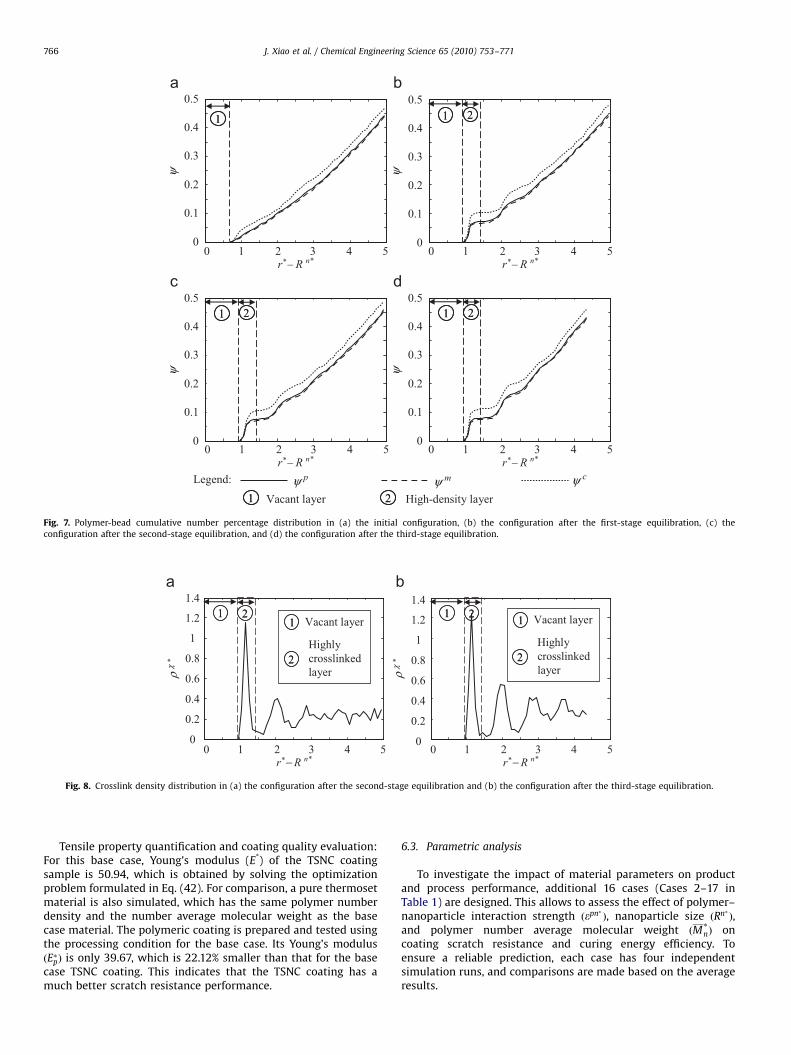
Microstructure analysis. Four structures shown in Fig. 4 possessa common feature: rp� or cp begins to rise from 0 at a certaindistance away from the nanoparticle surface. It means that thereexists a vacant layer next to the nanoparticle surface. Beyond thisvacant layer, the effective monomers and crosslinkers distributedifferently in the four structures.

In the initial structure, the distribution of polymer beads isrelatively uniform. As shown in Fig. 6(a), rp� is slightly fluctuatedaround a bulk density of 0.7989 (i.e., the initial setting for thepolymer-bead ND presented in Table 1). The uniform distributionis also confirmed in Fig. 7(a), where cp increases nearly linearlywith the distance.

After the first-stage equilibration, the shape of the distributioncurves changes dramatically. Fig. 6(b) shows that a high-polymer-density layer forms next to the vacant layer. This layer starts at thedistance of 0.95 from the nanoparticle surface and has a width of0.5. A prominent peak occurs at the distance of 1.15 to thenanoparticle surface, where both the effective monomers and thecrosslinkers reach their highest number densities. The maximumvalue of rp� reaches 5.535, which is 6.9 times greater than thebulk density of 0.7989. The formation of this high-density layer isdue to the aggregation of a noticeable number of effectivemonomers and crosslinkers during equilibration. As shown inFig. 7(b), this layer accumulates 7.2% of the polymer beads withthe distance range of 0.95–1.45 to the surface of the nanoparticle.On the other hand, only 5.5% of the polymer beads are initiallyallocated within the same distance range to the nanoparticlesurface (see Fig. 7(a)). In detail, the effective monomers in thelayer are increased from 5.2% by 1.5%, while the crosslinkers are

increased from 7.5% by 2.8%. It shows that the crosslinkers have ahigher propensity to aggregate towards the nanoparticle surface.

As shown in Fig. 6(b) and (c), the polymer-bead numberdensity distribution patterns after the first and the secondequilibration are very similar, but the maximum number densityof the effective monomers ðrm� Þ and that of the crosslinkers ðrc� Þ

are decreased by 9.5% and 14.1%, respectively, after the secondequilibration. On the other hand, the effective monomers andthe crosslinkers in the high-density layer are slightly increasedfrom 6.67% to 7.03% and from 10.32% to 10.53%, respectively (seeFig. 7(b) and (c)). These findings evidently show that duringcuring, more effective monomers than the crosslinkers, percen-tage wise move into the high-density layer, which means amoderate redistribution of the polymer beads. These help toachieve a high crosslinking conversion.

It is interesting to note that the high-density layer in Fig. 6(c) isa highly crosslinked layer shown in Fig. 8(a), and it possesses ahigh number density of EEJPs. Also note that the third-stageequilibration (after cooling) makes the heavily crosslinked layereven more concentrated. The maximum number density and thenumber percentage of the effective monomers and those of thecrosslinkers in the layer are all slightly increased (see Figs. 6(d)and 7(d)). The same trend is found for the crosslink density (seeFig. 8(b)). The volume shrinkage of the coating after coolingcontributes to the increase of the polymer bead number densityand crosslink density.

Coating testing and quality evaluation. The tensile test isconducted at the temperature of 0.75 and the pressure of 0. Thecoating sample is stretched in the required directions at aconstant strain rate until reaching the maximum strain of 5%.The constant strain increment of 0.05% is applied once every 10MC cycles, which indicates a strain rate of 0.005% MCC�1.According to Papakonstantopoulos et al. (2005), polymer nano-composites have glass transition temperature T�g of around 0.4, at

ARTICLE IN PRESS

0 1 2 3 4 50

1

2

3

4

5

6

711

ρ*ρ*

ρ*ρ*

0 1 2 3 4 50

1

2

3

4

5

6

711 22

0 1 2 3 4 50

1

2

3

4

5

6

711 22

0 1 2 3 4 50

1

2

3

4

5

6

711 22

*mρ *cρ*pρ

11 22Vacant layer High-density layer

Legend:

r*− R n* r*− R n*

r*− R n* r*− R n*

Fig. 6. Polymer-bead number density distribution in (a) the initial configuration, (b) the configuration after the first-stage equilibration, (c) the configuration after the

second-stage equilibration, and (d) the configuration after the third-stage equilibration.

J. Xiao et al. / Chemical Engineering Science 65 (2010) 753–771 765

which the number density of polymer beads is �1.01. In this casestudy, the TSNC coating sample to be tested is at the temperatureof 0.75, which is above T�g , at which the polymer bead numberdensity is 0.944. It indicates that this sample is in a rubbery state.

Stress–strain behavior: Stress evolution during tensile tests iscritical for mechanical property quantification. To obtain insightsinto the origin of the stress and to have a deep and comprehensiveunderstanding on the deformation behavior of a TSNC material,stress partitioning should be studied to differentiate the con-tributions by different types of stresses. The known studies onstress partitioning are only for studying the deformation behaviorof amorphous polymers (Chui and Boyce, 1999; Li et al., 2006;Mulder et al., 2007), but not for polymer nanocomposites.

The average normal stress in the tensile direction ðtÞ is givenby Eq. (43), while the average transverse normal stress ðtt

Þ isdefined as

tt¼

1

3

tyyx þtzz

x

2þtxx

y þtzzy

2þtxx

z þtyyz

2

� �ð45Þ

Fig. 9(a) plots two types of reduced stresses (t� and tt� ) as afunction of strain (x). It is shown that t� increases nearly linearlybefore x reaches �0.025, and its further increment becomes low,but tt� fluctuates around zero, which is at the pre-specifiedpressure. This means that the simulation is under excellentcontrol over the transverse stress in the tensile test. Fig. 9(b) givesthe behavior of the partitioned stresses against strain. As a note, apositive stress value indicates an attractive stress, while a

negative one is a repulsive stress. This figure provides thefollowing important information:

(i)

Type I stress—tI� (between the nonbonded polymer beads) isalways attractive. This means that the average distance betweenany pair of nonbonded polymer beads during a tensile test isalways greater than the minimum-energy distance (i.e., 1.12).

�

(ii)

Type II stress—tII (between the bonded polymers) is alwaysrepulsive, but its magnitude ðjt II�

jÞ is decreased along thestrain. This indicates that the bond is stretched. When twobonded polymer beads are repulsive to each other, increasingthe distance between them (i.e., the bond length) willdecrease the magnitude of the repulsive stress.

�

(iii)

Type III stress—tIII (between the polymer beads and thenanoparticle) is always attractive, but its magnitude isincreased only slightly along the strain. It indicates that theaverage polymer–nanoparticle surface distance is alwayslarger than 1.12 (i.e., the minimum-energy distance in apolymer–nanoparticle potential). The increase of the stress isa result of the increase of average polymer–nanoparticledistance, i.e., the polymer beads are pulled away from thenanoparticle surface during a tensile test.

�

(iv)

Type IV stress—tIV (between the nanoparticles) is always zero,because only one nanoparticle is involved in this case.

Overall, Type II stress causes the most significant stressfluctuation as compared to the others.

ARTICLE IN PRESS

0

0.1

0.2

0.3

0.4

0.5

11

ψ

0

0.1

0.2

0.3

0.4

0.5

ψ

11 22

0

0.1

0.2

0.3

0.4

0.5

ψ

11 22

0

0.1

0.2

0.3

0.4

0.5

ψ

11 22

Legend: 11 22Vacant layer High-density layer

ψ p ψ m ψ c

0 1 2 3 4 5r*− R n*

0 1 2 3 4 5r*− R n*

0 1 2 3 4 5r*− R n*

0 1 2 3 4 5r*− R n*

Fig. 7. Polymer-bead cumulative number percentage distribution in (a) the initial configuration, (b) the configuration after the first-stage equilibration, (c) the

configuration after the second-stage equilibration, and (d) the configuration after the third-stage equilibration.

0

0.2

0.4

0.6

0.8

1

1.2

1.411 22

ρχ

*

11 Vacant layer

22Highly crosslinkedlayer

0

0.2

0.4

0.6

0.8

1

1.2

1.411 22

ρχ

*

11 Vacant layer

22Highly crosslinkedlayer

0 1 2 3 4 5r*− R n*

0 1 2 3 4 5r*− R n*

Fig. 8. Crosslink density distribution in (a) the configuration after the second-stage equilibration and (b) the configuration after the third-stage equilibration.

J. Xiao et al. / Chemical Engineering Science 65 (2010) 753–771766

Tensile property quantification and coating quality evaluation:For this base case, Young’s modulus (E*) of the TSNC coatingsample is 50.94, which is obtained by solving the optimizationproblem formulated in Eq. (42). For comparison, a pure thermosetmaterial is also simulated, which has the same polymer numberdensity and the number average molecular weight as the basecase material. The polymeric coating is prepared and tested usingthe processing condition for the base case. Its Young’s modulusðE�pÞ is only 39.67, which is 22.12% smaller than that for the basecase TSNC coating. This indicates that the TSNC coating has amuch better scratch resistance performance.

6.3. Parametric analysis

To investigate the impact of material parameters on productand process performance, additional 16 cases (Cases 2–17 inTable 1) are designed. This allows to assess the effect of polymer–nanoparticle interaction strength ðepn� Þ, nanoparticle size ðRn� Þ,and polymer number average molecular weight ðM

�

nÞ oncoating scratch resistance and curing energy efficiency. Toensure a reliable prediction, each case has four independentsimulation runs, and comparisons are made based on the averageresults.

ARTICLE IN PRESS

0 0.01 0.02 0.03 0.04 0.05

−

−1

0.5

0

0.5

1

1.5

2

ξ

τ*

*τ

*tτ

0 0.01 0.02 0.03 0.04 0.05

*τ

*Iτ

*IIτ

*IIIτ

*IVτ

ξ

τ*

−

−1

0.5

0

0.5

1

1.5

2

Fig. 9. Stress–strain behavior: (a) average normal stress and average transverse normal stress as a function of strain and (b) partitioning of stresses.

*mρ *cρ*pρ 11 22Vacant layer High-density/highly crosslinked layerLegend: , ψ p , ψ m , ψ c

0 1 2 3 4.5

ρχ

*ρ

*ψ

ρχ

*ρ

*ψ

ρχ

*ρ

*ψ

1 2

r*− R n*r*− R n*0 1 2 3 4.5

1 2

0

0.4

0.8

1.2

0

0

0.2

0.4

2

4

6

0

0.4

0.8

1.2

0

0

0.2

0.4

2

4

6

0

0

0.2

0.4

2

4

6 11 22

r*− R n*

0

2

4

6

0

0.2

0.4

0

0.4

0.8

1.2

11 22

0 1 2 3 4.5 0 1 2 3 4.5

1

r*− R n*r*− R n*0 1 2 3 4.5

0

0

0.2

0.4

2

4

6

0

0.4

0.8

1.2

0

0

0.2

0.4

2

4

6

0

0.4

0.8

1.2

11

Fig. 10. Distributions of the polymer-bead number density (r*), cumulative number percentage (c), and crosslink density ðrw� Þ as a function of the polymer–nanoparticle

interaction strength for (a) Case 1 ðepn� ¼ 8:0Þ, (b) Case 4 ðepn� ¼ 4:0Þ, and (c) Case 2 ðepn� ¼ 0:4Þ.

J. Xiao et al. / Chemical Engineering Science 65 (2010) 753–771 767

Effect of epn� on product performance. Cases 2–6, together withCase 1, are designed to have different polymer–nanoparticleinteraction strengths, which is reflected by the value of the energyparameter ðepn�A ½0:4216:0�Þ (see Table 1). The TSNC coatingsamples are prepared and tested under the condition the same asthat for Case 1. For simplicity, the analysis of microstructure andstress–strain behavior below are only for Case 1 ðepn� ¼ 8:0Þ, Case 2ðepn� ¼ 0:4Þ, and Case 4 ðepn� ¼ 4:0Þ.

Coating microstructure: The microstructures of the unde-formed coating samples in Cases 1, 2 and 4 are characterizedbased on the distributions of the polymer-bead number densityðr�Þ, the cumulative number percentage (c), and the crosslinkdensity ðrw� Þ. As shown in Fig. 10(a), the microstructure in Case 1contains a prominent high-density layer, and the crosslinkers showa higher propensity to aggregate towards the nanoparticle surface

than the effective monomers. In that layer, cc reaches 11.18%, andcm is only 7.45%. In Case 4 (see Fig. 10(b)), the high-density layerbecomes less prominent, with the maximum rp� of 4.30 (29%lower than that in Case 1). The crosslinkers do not have a clearhigher propensity to aggregate towards the nanoparticle surfacethan the effective monomers. Note that Case 2 shows a completelydifferent distribution (see Fig. 10(c)), as there is no high-densitylayer and the polymer beads are more or less uniformlydistributed. Note that the difference of the rw� distributions inthree cases is also clear. The maximum rw� are 1.246 for Case 1 and0.935 for Case 4; all appear in the highly crosslinked layer. But thisis not the case for Case 2 as there is no such a layer.

The above analysis reveals that decreasing the polymer–nanoparticle interaction strength can give rise to: (i) a lessprominent high-density layer, (ii) a reduction of the number of

ARTICLE IN PRESS

J. Xiao et al. / Chemical Engineering Science 65 (2010) 753–771768

polymer beads in the high-density layer, (iii) a less prominenthighly crosslinked layer, and eventually (iv) a uniform distributionof polymer beads and EEJPs.

Stress-strain behavior: It is found that the polymer–nanoparticle stress ðtIII�

Þ in Case 1 is greater than the other twocases. This indicates that in order to have more contributions fromthe polymer–nanoparticle stress, a greater polymer–nanoparticleinteraction strength ðepn� Þ should be imposed.

Tensile property quantification and quality evaluation: Thecorrelation between E�=E�p and epn� is presented by a regressioncurve based on the results of Cases 1–6 (see Fig. 11). The detaileddata of E�=E�p with the mean value and standard deviation for allsix cases are listed in Table 1. It shows clearly that when epn� isincreased (i.e., the polymer–nanoparticle interaction strength is

*mρ *cρ*pρLegend: , ψ p , ψ m ,

0 1 2 3 4.5

ρ*

ψρ

χ*

ρ*

ψρ

χ*

1 2

0 1 2 3 4.5r*− R n*r*− R n*

0

0

0.2

0.4

0.6

0.8

1

2

4

6

0

0.4

0.8

1.2

0

0

0.2

0.4

0.6

0.8

1

2

4

6

0

0.4

0.8

1.2

11 22

0 1.5

1 2

0 1.5 3.53.5r*r*

0

0.2

0.4

0.6

0.8

10

2

4

6

0

0.4

0.8

1.2

0

0.2

0.4

0.6

0.8

10

2

4

6

0

0.4

0.8

1.2

11 22

Fig. 12. Distributions of the polymer-bead number density (r*), cumulative number per

(a) Case 1 ðRn� ¼ 7:00Þ, (b) Case 10 ðRn� ¼ 3:50Þ, and (c) Case 7 ðRn� ¼ 2:33Þ.

0 4 8 12 16 180.8

1

1.2

1.4

*pnε

E/E

E*/E* p

deterioration

enhancement

Fig. 11. Dependence of Young’s modulus of the TSNC coating on the polymer–

nanoparticle interaction strength.

enhanced), E* is increased as well and thus the tensile property/scratch resistance performance is improved. Fig. 11 also showsthat adding nanoparticles into a conventional thermoset materialdoes not guarantee enhancement of coating performance. A key toachieving performance improvement is to ensure that thepolymer–nanoparticle interaction strength ðepn� Þ is greater thana critical value (1.2 in this case, see Fig. 11).

Effect of Rn� on product performance. Six new cases (Case 7–12)are designed to explore the quantitative correlation betweennanoparticle size and coating performance, as compared to Case 1.As shown in Table 1, the only material parameter different fromeach other is the radius of nanoparticles ðRn� Þ. Note that the same-size simulation box is used for all cases. In order to achieve thesame nanoparticle volume fraction (fn=10.39%) and polymernumber density ðrp� ¼ 79:89%Þ, the numbers of nanoparticlesinvolved in Cases 1 and 7–12 are, respectively, 1, 27, 18, 12, 8, 4,and 2. The coating samples are prepared and tested under thesame condition as that for the base case. For simplicity, Case 1ðRn� ¼ 7:00Þ, Case 7 ðRn� ¼ 2:33Þ, and Case 10 ðRn� ¼ 3:50Þ areselected for analysis below.

Coating microstructure: As shown in Fig. 12, in each case, thecrosslinkers have a higher propensity than the effectivemonomers to move towards the nanoparticle surface (see the ccurves in Fig. 12, where the dotted line is above the dashed line ineach high-density layer). The number percentages of the polymerbeads within the high-density layers are, respectively, 7.97%,19.93%, and 35.31% for Cases 1, 10, and 7.

The study shows that the nanoparticle size has a minorinfluence on the polymer-bead r� distribution and rw� distribu-tion, but it plays a major role on the c distribution. Decreasing thenanoparticle radius can cause a significant increase in the numberpercentage of polymer beads within the high-density layer. One

11 22Vacant layer High-density/highly crosslinked layerψ c

ρ*

ψρ

χ*

885.55.5− R n*− R n*

0 1.67 3.67 5.67 7.67 9.17

1 2

0 1.67 3.67 5.67 7.67r*− R n*r*− R n*

9.17

0

0

0.2

0.4

0.6

0.8

1

2

4

6

0

0.4

0.8

1.2

0

0

0.2

0.4

0.6

0.8

1

2

4

6

0

0.4

0.8

1.2

11 22

centage (c), and crosslink density ðrw� Þ as a function of the nanoparticle radius for

ARTICLE IN PRESS

1.4

J. Xiao et al. / Chemical Engineering Science 65 (2010) 753–771 769

reason is the difference of the total surface areas of nanoparticles.For the systems having the nanoparticle radii of 7.00, 3.50, and2.33, the total surface areas of the nanoparticles are 616, 1,232,and 1,847, respectively.

Stress–strain behavior: It is found that the nanoparticle sizehas a very small influence on the polymer–polymer bonded stressðtII�Þ and the nanoparticle–nanoparticle stress ðtIV�

Þ. The differ-ence of the total stresses ðt�Þ in the three cases is mainly due tothe difference of the polymer–nanoparticle stresses ðtIII�

Þ and thepolymer–polymer nonbonded stresses ðtI�

Þ. Decreasing nanopar-ticle size makes tIII� increased in the whole range of strain understudy. This can be understood by checking the c distributions inthese cases (see Fig. 12). In the high-density layer, the c value forCase 7 (using the smallest nanoparticles) is larger than that for theother two cases; this causes a greater polymer–nanoparticlestress. It is also noticed that when smaller nanoparticles are used,

2 3 4 5 6 71.2

1.3

1.4

1.5

*nR

E*/E* p

E*/E* p

Fig. 13. The effect of nanoparticle size on Young’s modulus of the TSNC coating.

0 1 2 3 4.5

0

0

0.2

0.4

2

4

6

0

0.4

0.8

1.2

1.6

1 2

0 1 2 3 4.5r*− R n*r*− R n*

0

0

0.2

0.4

ρρ*ψ

2

4

6

0

0.4

0.8

1.2

1.6

ρ*

ρχ

*

ρρ*ψ

ρ*

ρχ

*

11 22 1 2

0 1 2

11 22

0

0

0.2

0.4

2

4

6

0

0.4

0.8

1.2

1.6

0

0

0.2

0.4

2

4

6

0

0.4

0.8

1.2

1.6

0 1 2r*r*

*mρ *cρ*pρLegend: , ψ p , ψ m

Fig. 14. Distributions of the polymer-bead number density (r*), cumulative number perc

molecular weight for (a) Case 17 ðM�

n ¼ 16:68Þ, (b) Case 1 ðM�

n ¼ 8:34Þ, and (c) Case 13 ð

the stress between the nonbonded polymer beads ðtI�Þ becomes

smaller throughout the range of the strain studied. The reason forthis phenomenon is yet to be investigated.

Tensile property quantification and quality evaluation: Fig. 13provides the relationship between E�=E�p and Rn� . It shows thatusing smaller nanoparticles can improve the tensile property ofthe TSNC coating and thereby scratch resistance performance. Theimprovement will be more significant when the nanoparticles aremuch smaller. This is difficult to be explained using thecontinuum mechanics theory, but can be readily understoodwhen examining the microstructures and the stress partitioning.

Effect of M�

n on product performance: The performance of a TSNCcoating heavily depends on the type of polymeric material used.

ρρ*ψ

ρ*

ρχ

*

3 4.53 4.5− R n*− R n*

0 1 2 3 4 4.5

1 2

0 1 2 3 4 4.5

1 2

0 1 2 3 4 4.5r*− R n*r*− R n*r*− R n*

0

0.2

0.4

0

2

4

6

0

0.4

0.8

1.2

1.60

0.2

0.4

0

2

4

6

0

0.4

0.8

1.2

1.60

0.2

0.4

0

2

4

6

0

0.4

0.8

1.2

1.6

11 22

11 22Vacant layer High-density/highly crosslinked layer, ψ c

entage (c), and crosslink density ðrw� Þ as a function of the polymer number average

M�

n ¼ 2:78Þ.

2 6 10 14 180.9

1

1.1

1.2

1.3

E/E

E*/E* p

*nM

Fig. 15. Effect of the polymer number average molecular weight on Young’s

modulus of the TSNC coating.

ARTICLE IN PRESS

J. Xiao et al. / Chemical Engineering Science 65 (2010) 753–771770

In this regard, five new cases (Cases 13–17) are designed, wherethe polymer number average molecular weights are different fromeach other as well as Case 1 (see Table 1). In the following, Case 1ðM�

n ¼ 8:34Þ, Case 13 ðM�

n ¼ 2:78Þ, and Case 17 ðM�

n ¼ 16:68Þ areselected for a more detailed investigation.

Coating microstructure: The r� and c distributions for Cases17, 1, and 13 are plotted in Fig. 14, where no major difference canbe observed. However, this is not the case for the rw� distribution;the rw� always has a greater value when M

�

n is greater. Thissuggests that M

�

n has a negligible effect on the distributions ofeffective monomers and crosslinkers, but has a pronouncedinfluence on the distribution of EEJPs. The crosslink density, orthe number density of EEJPs, increases along M

�

n. This is becausefor the same conversion the chance for a polymer bead to be anEEJP in a higher M

�

n system is much greater than that in a lowerM�

n system.

2 6 14 180.6

0.8

1

1.2

1.4

10*nM

2 3 4 5 6 70.8

1

1.2

1.4

1.6

2 3 4 5 6 70.8

1

1.2

1.4

1.6

*nR *nR

0 4 8 12 16 180.95

1

1.05

1.1

1.15

0 4 8 12 16 180.95

1

1.05

1.1

1.15

*pnε *pnε

N/N

N/N

NMCC/NMCC

pN

/NN

/NNMCC/NMCC

pN

/NN

/NNMCC/NMCC

p

Fig. 16. Curing time dependence on (a) the polymer–nanoparticle interaction

strength, (b) the nanoparticle radius, and (c) the polymer number average

molecular weight.

Stress–strain behavior, tensile property, and quality evaluation:Simulation shows that the selection of M

�

n has almost no effect onthe polymer–nanoparticle stress ðtIII�

Þ and the nanoparticle–nanoparticle stress ðt IV�

Þ, but is relatively sensitive to the slopeof the polymer–polymer bonded stress ðtII�

Þ when the strain iso2%. This makes the overall stress curves ðt�Þ different,particularly for a smaller M

�

n. Fig. 15 shows how Young’smodulus (E*) behaves as the polymer number average molecularweight ðM

�

nÞ changes. Clearly, the TSNC coating scratch resistanceis more robust when M

�

n is larger, and thus that the crosslinkdensity in the system is greater (see Fig. 14).

Effect on process performance. Another uniqueness of theintroduced methodology is its capability of identifying opportu-nities for improving processing efficiency. The processing effi-ciency considered in this work is evaluated by the time needed forcuring the TSNC coating to a specific crosslinking conversionpercentage. If the pattern of the curing temperature profile (or theheating policy) is given (see Fig. 5(b)), and the time duration forcuring at temperature T*=1 is adjustable, it is certain that thelonger the time duration, the higher the energy consumption.

Note that in MC simulation, the curing time elapsed can bereflected by the MC cycles used. Their exact correlation, however,is difficult to derive, because for any specific MC cycle, itsequivalence of real curing time varies. But it is certain that moreMC cycles imply a longer curing time and thus more energy

required. Fig. 16 demonstrates how the ratio of NMCC to NMCCp

changes for a material that is characterized by epn� , Rn� , or M�

n;

where NMCC and NMCCp are, respectively, the needed number of MC

cycles for the TSNC coating and that for the pure-polymer coatingto reach 80% of crosslinking conversion. It is shown that to reduceenergy consumption for coating curing, the nanomaterial should

have a smaller epn� and M�

n, but a larger Rn�. However, according to

the discussion in the previous sections, such a type of material canlead to a less or even much less superior performance on scratchresistance (see the summarized data in Table 1). Consequently,material designers should be prepared to make trade-offsbetween product performance and processing efficiency. Thisintroduced methodology can provide detailed, quantitativeinformation for the purpose.

7. Conclusions and future work

Thermoset nanocomposites (TSNCs) are the polymer compositematerials that can significantly improve appealing properties andoffer new functionalities in the resulting coatings. However, howto effectively and efficiently design TSNCs to achieve anticipatedcoating properties and performance as well as material processingefficiency is an extremely challenging task. The computationalmethodology introduced in this work is probably among the firstof this kinds for TSNC material design. The 3D simulation andstructural and parametric analysis techniques can provide materialdesigners with various types of insightful information, and helpgain a comprehensive and deep understanding on how the TSNCsformulation can influence coating property and energy efficiency.This is also among the earliest efforts on stress partitioning whenstudying the deformation of TSNCs. Through examining thecontributions by different stresses, the deformation behavior ofthe material can be clearly visualized.

The developed methodology builds a solid basis for the futurestudy on optimal TSNC coating design. Undoubtedly, morecomprehensive and sophisticated studies are needed. The meth-odology is currently being extended for characterizing TSNCsusing different shapes of nanoparticles. In analyzing the stress–strain behavior, a large strain will be imposed so that other

ARTICLE IN PRESS

J. Xiao et al. / Chemical Engineering Science 65 (2010) 753–771 771

properties, e.g., yield strength and yield strain, can be quantified.Furthermore, quantitative correlations between the scratchresistance and various properties need to be developed. Othercoating performance, such as corrosion prevention, appearance,and inter-coat adhesion, should also be investigated. Needless tosay, all the correlations and design improvement strategiesidentified through simulation must be experimentally validated.

Acknowledgments

This work is supported in part by NSF (CMMI 0700178) and theInstitute of Manufacturing Research of Wayne State University.

References

Adnan, A., Sun, C.T., Mahfuz, H., 2007. A molecular dynamics simulation study toinvestigate the effect of filler size on elastic properties of polymernanocomposites. Compos. Sci. Technol. 67, 348–356.

Allen, M.P., Tildesley, D.J., 1987. Computer Simulation of Liquids. Clarendon Press,Oxford.

Bedrov, D., Smith, G.D., Smith, J.S., 2003. Matrix-induced nanoparticle interactionsin a polymer melt: a molecular dynamics simulation study. J. Chem. Phys. 119,10438–10447.

Bharadwaj, R.K., Mehrabi, A.R., Hamilton, C., Trujillo, C., Murga, M., Fan, R., Chavira,A., Thompson, A.K., 2002. Structure–property relationships in cross-linkedpolyester–clay nanocomposites. Polymer 43, 3699–3705.

Cho, J., Sun, C.T., 2007. A molecular dynamics simulation study of inclusion sizeeffect on polymeric nanocomposites. Comput. Mater. Sci. 41, 54–62.

Chui, C., Boyce, M.C., 1999. Monte Carlo modeling of amorphous polymerdeformation: evolution of stress with strain. Macromolecules 32, 3795–3808.

Dionne, P.J., Picu, C.R., Ozisik, R., 2006. Adsorption and desorption dynamics oflinear polymer chains to spherical nanoparticles: a Monte Carlo investigation.Macromolecules 39, 3089–3092.

Frankland, S.J.V., Harik, V.M., Odegard, G.M., Brenner, D.W., Gates, T.S., 2003. Thestress–strain behavior of polymer–nanotube composites from moleculardynamics simulation. Compos. Sci. Technol. 63, 1655–1661.

Garces, J.M., Moll, D.J., Bicerano, J., Fibiger, R., McLeod, D.G., 2000. Polymericnanocomposites for automotive applications. Adv. Mater. 12, 1835–1839.

Gina, N., Cohen, C., Panagiotopoulos, A.Z., 2000. A Monte Carlo study of thestructural properties of end-linked polymer networks. J. Chem. Phys. 112,6910–6916.

Holzl, T., Wittkop, M., Kreitmeier, S., Goritz, D., 1997. Uniaxial deformation ofbridging polymer systems: a Monte Carlo study. J. Chem. Phys. 106, 7792–7801.

Hosseinpour, D., Guthrie, J.T., Berg, J.C., Stolarski, V.L., 2005. The effect of interfacialinteraction contribution to the mechanical properties of automotive topcoats.Prog. Organic Coatings 54, 182–187.

Humphrey, W., Dalke, A., Schulten, K., 1996. VMD—visual molecular dynamics.J. Mol. Graphics 14, 33–38.

Jalili, M.M., Moradian, S., Dastmalchian, H., Karbasi, A., 2007. Investigating thevariations in properties of 2-pack polyurethane clear coat through separateincorporation of hydrophilic and hydrophobic nano-silica. Prog. OrganicCoatings 59, 81–87.

Kotsikova, R. (Ed.), 2007. Thermoset Nanocomposites for Engineering Applications.Smithers Rapra Technology, UK.

Kremer, K., Grest, G.S., 1990. Dynamics of entangled linear polymer melts: amolecular dynamics simulation. J. Chem. Phys. 92, 5057–5086.

Kutschera, M., Sander, R., 2006. Scratch resistance of automobile clearcoat:chemistry and characterization on the micro- and nanoscale. JCT Research 3,91–97.

Li, J., Mulder, T., Vorselaars, B., Lyulin, A.V., Michels, M.A.J., 2006. Monte Carlosimulation of uniaxial tension of an amorphous polyethylene-like polymerglass. Macromolecules 39, 7774–7782.

Metropolis, N., Rosenbluth, A.W., Rosenbluth, M.N., Teller, A.H., Teller, E., 1953.Equation of state calculations by fast computing machines. J. Chem. Phys. 21,1087–1092.

Miller, D.R., Macosko, C.W., 1976. A new derivative of post gel properties ofnetwork polymers. Macromolecules 9, 206–211.

Misra, R.D.K., Hadal, R., Duncan, S.J., 2004. Surface damage behavior during scratchdeformation of mineral reinforced polymer composites. Acta Mater. 52,4363–4376.

Mulder, T., Li, J., Lyulin, A.V., Michels, M.A.J., 2007. Monte Carlo simulation ofuniaxial deformation of polyethylene-like polymer glass: role of constraintsand deformation protocol. Macromol. Theory Simul. 16, 348–358.

Nobel, M.L., Picken, S.J., Mendes, E., 2007. Waterborne nanocomposite resin forautomotive coating applications. Prog. Organic Coatings 58, 96–104.

Ozmusul, M.S., Picu, C.R., Sternstein, S.S., Kumar, S.K., 2005. Lattice Monte Carlosimulations of chain conformations in polymer nanocomposites. Macromole-cules 38, 4495–4500.

Papakonstantopoulos, G.J., Yoshimoto, K., Doxastakis, M., Nealey, P.F., de Pablo, J.J.,2005. Local mechanical properties of polymeric nanocomposites. Phys. Rev. E72, 031801-1–031801-6.

Pluart, L.L., Duchet, J., Sautereau, H., 2005. Epoxy/montmorillonite nanocompo-sites: influence of organophilic treatment on reactivity, morphology andfracture properties. Polymer 46, 12267–12278.

Ryntz, R.A., Britz, D., 2002. Scratch resistance behavior of automotive plasticcoatings. JCT 74, 77–81.

Shen, W., Smith, S.M., Jones, F.N., Ji, C., Ryntz, R.A., Everson, M.P., 1997. Use of ascanning probe microscope to measure marring mechanisms and microheard-ness of crosslinked coatings. JCT 69, 123–135.

Sheng, N., Boyce, M.C., Parks, D.M., Rutledge, G.C., Abes, J.I., Cohen, R.E., 2004.Multiscale micromechanical modeling of polymer/clay nanocomposites andthe effective clay particle. Polymer 45, 487–506.

Starr, F.W., Schroder, T.B., Glotzer, S.C., 2002. Molecular dynamics simulation of apolymer melt with a nanoscopic particle. Macromolecules 35, 4481–4492.

Vacatello, M., 2001. Monte Carlo simulations of polymer melts filled with solidnanoparticles. Macromolecules 34, 1946–1952.

Vacatello, M., 2002. Molecular arrangements in polymer-based nanocomposites.Macromol. Theory Simul. 11, 757–765.

Valavala, P.K., Odegard, G.M., 2005. Modeling techniques for determinationof mechanical properties of polymer nanocomposites. Rev. Adv. Mater. Sci. 9,34–44.

Wittkop, M., Sommer, J.U., Kreitmeier, S., Goritz, D., 1994. Monte Carlo simulationof a single polymer chain under an external force in two and three dimensions.Phys. Rev. E 49, 5472–5476.

Xiao, J., Huang, Y.L., 2009. Microstructure-property-quality-correlated paintdesign: an LMC-based approach. A.I.Ch.E. J. 55, 132–149.

Yang, L., Srolovitz, D.J., Yee, A.F., 1997. Extended ensemble molecular dynamicsmethod for constant strain rate uniaxial deformation of polymer systems.J. Chem. Phys. 107, 4396–4407.

Zeng, Q.H., Yu, A.B., Lu, G.Q., 2008. Multiscale modeling and simulation of polymernanocomposites. Prog. Polymer Sci. 33, 191–269.

Zhang, Q., Archer, L.A., 2004. Monte Carlo simulation of structure and nanoscaleinteractions in polymer nanocomposites. J. Chem. Phys. 121, 10814–10824.