computation of implied dividend based on option...

Computation of implied dividend based on option

market data

Qi Cao

September 26, 2005

I really appreciate the the help from my superviser Kees Oosterlee, myColleagues Ariel Almendral, Jasper Anderluh, Coen Leentvaar and XinzhengHuang.

1

Contents

1 Introduction 4

2 Black-Scholes Analysis with European Options 62.1 Black-Scholes model without dividend . . . . . . . . . . . . . 62.2 Boundary and Initial conditions for European option . . . . . 82.3 Derive the Black-Scholes Formula . . . . . . . . . . . . . . . . 92.4 Put-Call Parity . . . . . . . . . . . . . . . . . . . . . . . . . . 122.5 Some option pricing models with discrete dividend . . . . . . 13

3 Black-Scholes Analysis for American Options 153.1 Basic idea of American Options . . . . . . . . . . . . . . . . . 153.2 American put option as free boundary problems . . . . . . . . 173.3 American options with discrete dividend . . . . . . . . . . . . 19

4 Finite-difference methods for pricing options 224.1 Difference Approximations . . . . . . . . . . . . . . . . . . . . 224.2 Explicit Method . . . . . . . . . . . . . . . . . . . . . . . . . 234.3 Implicit Method . . . . . . . . . . . . . . . . . . . . . . . . . 244.4 The Crank-Nicolson Method . . . . . . . . . . . . . . . . . . . 284.5 Discretization of the general form of the PDE . . . . . . . . . 29

4.5.1 Fourth order accuracy . . . . . . . . . . . . . . . . . . 304.5.2 Coordinate transformation with stretching . . . . . . . 31

4.6 Methods for American Options . . . . . . . . . . . . . . . . . 33

5 Parameter Study based on Black-Scholes Equation 375.1 Effect of single dividend and interest rate . . . . . . . . . . . 375.2 Effect of two dividends and interest rate . . . . . . . . . . . . 395.3 Effect of the parameters using volatility adjustment . . . . . 41

5.3.1 Effect of single dividend and interest rate using volatil-ity adjustment . . . . . . . . . . . . . . . . . . . . . . 41

5.3.2 Effect of two dividends and interest rate using volatil-ity correction . . . . . . . . . . . . . . . . . . . . . . . 43

2

6 Calibration of the Implied Variables 456.1 Implied volatility and implied dividend . . . . . . . . . . . . . 466.2 Calibration Methods . . . . . . . . . . . . . . . . . . . . . . . 476.3 Comparison of fmincon and fminsearch . . . . . . . . . . . . . 506.4 Algorithm of the whole approach . . . . . . . . . . . . . . . . 516.5 Objective Functions . . . . . . . . . . . . . . . . . . . . . . . 526.6 Calibration Results . . . . . . . . . . . . . . . . . . . . . . . . 53

6.6.1 Single dividend from ING . . . . . . . . . . . . . . . . 536.6.2 Two dividends from ING . . . . . . . . . . . . . . . . 596.6.3 Calibrated parameters for Fortis option . . . . . . . . 63

7 Conclusion 69

3

Chapter 1

Introduction

Options are popularly traded in today’s financial market. They are oftenconnected to some item, such as a listed stock, an exchange index, futurescontracts, or real estate. In this thesis, the stock option is discussed. Thereare two basic types of options, the European and American. A Europeanoption is an option contract that can only be exercised on the expirationdate. Futures contracts (i.e., options on commodities) are generally Euro-pean style options. An American option is an option contract that can beexercised at any time between the date of purchase and the expiration date.Most exchange-traded options are American-Style. Stock options are typi-cally American style.

The famous Black-Scholes model is a fast and effective way to calculatethe option price. An analytical solution for European options exist, how-ever, for the stock options which are American style, a numerical approach isnecessary. In real markets, many companies pay dividends to the stock hold-ers not to the option holders. Whereas, the classical Black-Scholes modelcannot deal with the dividend payment, so we use Wilmott’s model which isan improvement of the Black-Scholes model to include the discrete dividend.

Sometimes, the announcement of the amount of dividend payment and theex-dividend date cannot be obtained by the investors. At this time, thedividend is implied. To calculate the implied dividend as well as the impliedvolatility, two calibration methods are applied with the fixed risk-free inter-est rate. The data set is collected from the ING Group from Jan 2005 tillJun 2006.

In this thesis, the following issues are discussed. In chapter 2, the defi-nitions and properties of European options are discussed; the Black-Scholesequation is derived and some simple dividend payment models are intro-duced. In chapter 3, the properties of American options are discussed. In

4

chapter 4, some finite difference approximation methods for computing bothof the European and American styles option prices are introduced. In chap-ter 5, we illustrate how the option pricing parameters needed in the B-Smodel influence the option price. In chapter 6, two basic optimization ap-proaches for computing implied parameters are introduced and the resultsof the thesis are presented.

5

Chapter 2

Black-Scholes Analysis withEuropean Options

2.1 Black-Scholes model without dividend

With European Options: the holder of the option has the right, not theobligation to buy (call) or to sell (put), at a fixed date (expiry date) for afixed price (exercise price) an asset (share, goods, derivative).

The value V (premium) of an option (C for a call, P for a put) will de-pend on the following parameters:

• present value of the asset S

• time t till expiry T

• volatility of asset

• the risk-free interest rate r

• the exercising price E

The Black-Scholes model is valid under the following assumptions:

• the asset price S follows a lognormal random walk

• the risk free interest rate r and the volatility σ of the assets are as-sumed constant for the entire life time of the option

• no transaction costs for portfolio-hedging are included

• no dividends are paid on the asset during the option contract

6

• there are no arbitrage possibilities

• trading with the underlying asset can be done continuously

• short selling is permitted, and the asset can be divided arbitrarily

The asset price S is assumed to follow a lognormal random walk, a simplemathematical formula for S is

dS

S= µdt + σdX (2.1)

Where µ is known as the drift, usually µ is constant and it represents theaverage rate of growth of the asset price. σ is defined as the volatility, whichmeasures the standard deviation of the return. Here both µ and σ are as-sumed to be constant. dX is a Wiener process, a normal distribution withmean 0 and variance dt, which describes the randomness of the asset price.

If f(S, t) is a smooth function in both S and t, discarding the stochasticmoment of S and t, expand f(S, t) by the Taylor series up to second orderterms, given

df =∂f

∂SdS +

∂f

∂tdt +

12(∂2f

∂S2dS2 + 2

∂2f

∂S∂tdSdt +

∂2f

∂t2dt2) + . . . (2.2)

dS is given by (2.1), so

dS2 = σ2S2dX2 + 2σµS2dtdX + µ2S2dt2 (2.3)

where dX2 = dt, and the other terms are of lower order. So that

df = σSdf

dSdX + (µS

df

dS+

12σ2S2 d2f

dS2dS2 +

∂f

∂t)dt (2.4)

Eq. (2.4) is called Ito’s lemma.

We suppose the option price V (S, t) satisfies Ito’s lemma defined by (2.4),so

dV (S, t) = σS∂V

∂SdX + (µS

∂V

∂S+

12σ2S2 ∂2V

∂S2+

∂V

∂t)dt (2.5)

To eliminate the stochastic part dX, we construct a portfolio consisting oneoption and −∆ assets. The value of this portfolio is

Π = V −∆S (2.6)

The change in portfolio dΠ reads:

dΠ = dV −∆dS (2.7)

7

Here ∆ is constant for dt, and Π then follows the random walk

dΠ = σS(∂V

∂S−∆)dX + (µS

∂V

∂S+

12σ2S2 ∂2V

∂S2+

∂V

∂t− µ∆S)dt (2.8)

Choosing ∆ = ∂V∂S the randomness can be eliminated to some extent, so

that a deterministic portfolio is obtained. Due to the absence of arbitrage,the return of the portfolio in dt must equal that of the risk-free bank account:

rΠdt = dΠ (2.9)

This leads to the famous Black-Scholes equation!

∂V

∂t+

12σ2S2 ∂2V

∂S2+ rS

∂V

∂S− rV = 0 (2.10)

Remarks:

• A derivative satisfying the above assumptions and which only dependson the present value S and t can be described by the Black-Scholesequation

• The value of an option is independent of the drift parameter µ

• The (linear) Black-Scholes operator

LBS =∂

∂t+

12σ2S2 ∂2

∂S2+ rS

∂

∂S− r (2.11)

has a financial interpretation as the difference between the hedgedportfolio and the return of a bank deposit.

2.2 Boundary and Initial conditions for Europeanoption

The Black-Scholes equation needs a final condition and boundary conditionsto derive the unique solution of the partial differential equation. For the Eu-ropean call, one can define a vanilla option value by C(S, t), with exerciseprice E and expiry date T .

The final condition at t = T , the value of call option is known to be thepayoff

C(S, T ) = max(S − E, 0) (2.12)

When S = 0, then dS = 0, so that the asset price doesn’t change during dt,

8

and at expiry the payoff is zero. We have

C(0, t) = 0 (2.13)

When S → ∞, the option will be exercised and the magnitude of exerciseprice is less important. So the option value becomes the asset value at thistime:

C(S, t) ∼ S −Ee−r(T−t) as S →∞ (2.14)

For a European call option, it is not possible to exercise early, (2.10) and(2.12)-(2.14) can be solved to give the Black-Scholes analytical solution ofthe call option.

For a put option, with value P (S, t), the final condition is the payoff

P (S, T ) = max(E − S, 0) (2.15)

Similar to the European call case, as S = 0, the final payoff of Europeanput is certainly E.P (0, t) is the present value of E received at T . Assumingthe risk-free interest rate is r, then

P (0, t) = Ee−r(T−t) (2.16)

As S ∼ ∞, the option is unlikely to be exercised, then

P (S, t) → 0 as S →∞ (2.17)

2.3 Derive the Black-Scholes Formula

A European call C(S, t) price given by the Black-Scholes equation can bewritten as:

∂C

∂t+

12σ2S2 ∂2C

∂S2+ rS

∂C

∂S− rC = 0 (2.18)

withC(0, t) = 0, C(S, t)− Ee−r(T−t) ∼ S at S →∞

andC(S, T ) = max(S − E, 0)

In order to transform (2.18) to a diffusion equation

∂u

∂τ=

∂2u

∂x2(2.19)

9

we need to set

S = Eex, t = T − τ/12σ2, C = Ev(x, τ) (2.20)

Then we get∂v

∂τ=

∂2v

∂x2+ (k − 1)

∂v

∂x− kv (2.21)

where k = r/12σ2, and the initial condition for v is

v(x, 0) = max(ex − 1, 0)

Then letv(x, τ) = eαx+βτu(x, τ) (2.22)

The two unknowns α and β needs to be solved, so put (2.22) to (2.21), anddifferentiate it, then

βu +∂u

∂τ= α2u + 2α

∂u

∂x+

∂2v

∂x2+ (k − 1)(αu +

∂u

∂x)− ku

To eliminate the terms of u and ∂u/∂x, we have

β = α2 + (k − 1)α− k, 0 = 2α + (k − 1)

then α and β are calculated as:

α = −12(k − 1), β = −1

4(k + 1)2

After these transformations, we finally substitute (2.18) into (2.19), where

v = e−12(k−1)x− 1

4(k+1)2τu(x, τ)

with the initial condition

u(x, 0) = u0(x) = max(e12(k+1)x − e

12(k−1)x, 0)

so that we obtain the diffusion equation:

∂u

∂τ=

∂2u

∂x2for −∞ < x < ∞, τ > 0

The solution of the diffusion equation is

u(x, τ) =1

2√

πτ

∫ ∞

−∞u0(S)e−(x−s)2/4τds (2.23)

10

To evaluate the integral in (2.23), make the transformation x′ = (s−x)/√

2τ ,we get

u(x, τ) =1

2√

π

∫ ∞

−∞u0(x′

√2τ + x)e−

12x′2dx′

=1

2√

π

∫ ∞

−x/√

2τe

12(k+1)(x+x′

√2τ)e−

12x′2dx′

− 12√

π

∫ ∞

−x/√

2τe

12(k−1)(x+x′

√2τ)e−

12x′2dx′

= I1 − I2

To evaluate I1 by completing the square in the component to get a standardintegral:

I1 =1

2√

π

∫ ∞

−x/√

2τe

12(k+1)(x+x′

√2τ)e−

12x′2dx′

=e

12(k+1)x

√2π

∫ ∞

−x/√

2τe

14(k+1)2τe−

12(x′− 1

2(k+1)

√2τ)2dx′

=e

12(k+1)x+ 1

4(k+1)2τ

√2π

∫ ∞

−x/√

2τ− 12(k+1)

√2τ

e−12η2

dη

= e12(k+1)x+ 1

4(k+1)2τN(d1),

whered1 =

x√2τ

+12(k + 1)

√2τ

and

N(d1) =1√2π

∫ d1

−∞e−

12s2

ds

The computation of I2 is similar to the approach of I1 except replacing(k + 1) by (k − 1). Recall that

v(x, τ) = e−12(k−1)x− 1

4(k+1)2τu(x, τ) (2.24)

and x = log(S/E), τ = 12σ2(T −t) so for a European call option the solution

of the BS equation reads

CE(S, t) = SN(d1)−Ee−r(T−t)N(d2) (2.25)

With N(x), the cumulative normal distribution function, and

d1 =log(S/E) + (r + 1

2σ2)(T − t)σ√

T − t(2.26)

d2 =log(S/E) + (r − 1

2σ2)(T − t)σ√

T − t(2.27)

11

2.4 Put-Call Parity

The Put-Call parity is a relationship, first identified by Stoll (1969), thatexists between the prices of European put and call options that both havethe same underlying, strike price and expiration date. The relationship isderived using arbitrage arguments. Consider two portfolios consisting of:

1.The call option and an amount of cash equal to the present value of thestrike price.

2.The put option and the underlying.

Comparing the expiration value for these two portfolios, with E representingthe common strike price, we find the following:

A portfolio comprising a call option and an amount x of cash equal to thepresent value of the option’s strike price has the same expiration value as aportfolio comprising the corresponding put option and the underlying. ForEuropean options, early exercise is not possible. If the expiration values ofthe two portfolios are the same, then their present values must also be thesame. This equivalence is the so-called Put-Call parity.

If the two portfolios are going to have the same value at expiration, thenthey must have the same value today. Otherwise, an investor can make anarbitrage profit by purchasing the less expensive portfolio, selling the moreexpensive one and holding the long-short position to expiration. Accord-ingly, we have the price equality:

c + Ee−r(T−t) = p + S (2.28)

Where c is the price of European call option, p is the price of Europeanput option, S is the asset price and r is the risk-free interest rate given theoption’s lifetime T and the time right now t.

Note that, the Put-Call parity applies only to European options, since apossibility of early exercise can cause a divergence in the present values ofthe two portfolios.

The Put-Call parity offers a simple test of option pricing models. Anyoption pricing model that produces put and call prices that do not satisfyput-call parity must be rejected as unsound. Such a model will suggesttrading opportunities where none exist.

12

2.5 Some option pricing models with discrete div-idend

During the life time of the option we have a single dividend payment D attd. Due to the absence of arbitrage:

S(t+d ) = S(t−d )−D (2.29)

where t+d and t−d are the instants immediately before and after the ex-dividend date. The value V of the option must be smooth as a functionof time over the time of payment

V (S(t+d ), t+d ) = V (S(t−d ), t−d ) (2.30)

We distinguish the following approaches to include a discrete dividend.

a. Wilmott’s method: This method is derived directly from (5.7) and(5.8), which follows the following steps:-solve BS differential equation backwards from expiry T to t+d-incorporate jump condition (5.7) and (5.8) to find value for t−d-solve BS differential equation backwards with this value as final conditionfrom t−d to t

Cd(S, t) = C(S, t, E), t+d ≤ t ≤ T

Cd(S, t−d ) = Cd(S −D, t+d ) = C(S −D, t+d , E)

C(S −D, t, E) is still a solution for all t ≤ t−d .

b. Back to Basics’s method [1]:In the ”Back to Basics” article, the extreme situation has been consideredfor paying dividend. For instance, the company want to pay S (liquidator)or 0 (survivor) for the dividend. Actually, we usually assume S, so today’sprice of a European call option can be calculated by the following integral:

CE(S, 0, D, td) = e−rtd

∫ ∞

DCBS(S −D, td)φ(S0, S, td)dS (2.31)

c. Volatility adjusted modelBased on the solution of BS equation, Merton (1973) used S − e−rtdD in-stead of S, which means the asset price is replaced by the difference of assetprice minus the discounted dividend D:

CE(S, 0, D, td) = (S − e−rtdD)N(d1)−Ee−rT N(d2) (2.32)

Because there is some jump in S, the volatility of the asset price will changeafter the dividend payment. To keep the volatility constant, there are some

13

methods to adjust it. From an adjusted S, one can derive the adjusted σdirectly:

σ(S, t,D) =

{σc

S−e−rtdDS (t ∈ [0, td])

σc (t ∈ [td, T ])(2.33)

σ(S, t,D) =

{σc (t ∈ [0, td])σc

S+e−rtdDS (t ∈ [td, T ])

(2.34)

In some situations, like the Japanese market, the interest rate is close to 0.The adjustment can be simplified to:

σ(S, t, D) =

{σc

S−DS (t ∈ [0, td])

σc (t ∈ [td, T ])

σ(S, t, D) =

{σc (t ∈ [0, td])σc

S+DS (t ∈ [td, T ])

In this situation, the option price produced by Wilmott’s method changes bytime, which is contrary to the real world, because the option price should beindependent of tD when r = 0. Applying the volatility adjusted approach,(2.33) or (2.34), we can get the unchanged option price C in the option’slifetime independent of tD.

When r 6= 0, each of the method performs well, whereas the option pricegiven by (2.34) is a bit higher than that by (2.33) for the volatility generatedby (2.34) is a bit larger than that by (2.33). There is also a drawback in ourmodel. For an American option, the price should be higher than its equiva-lent of a European option without dividend payment. But in the volatilityadjusted model, the European option is more expensive than the Americanoption when dividend payment is close to the expiry date.

14

Chapter 3

Black-Scholes Analysis forAmerican Options

3.1 Basic idea of American Options

An American Option is an option that can be exercised anytime during itslife time. The majority of exchange-traded options are American in the realmarket.

In fact, the American option holders have greater flexibility than the Eu-ropean counterpart, because of their right to exercise early. Therefore theAmerican options have typically higher values than the European equiva-lents. For the American call option,

C(S, t) ≥ max(S − E, 0)

and for the American put option,

P (S, t) ≥ max(E − S, 0)

In this case, during the life of the option there will be some values of S forwhich it is optimal for the holders to exercise the American option. Unlikethe European option, one may be interested in determining the value ofSf (t), for which it is optimal to exercise.

If there is no dividend paid during the option’s life time, the Americancall option is equal to the European call option, which means that it is notoptimal to exercise the American call option prematurely if the asset is non-dividend payment. And if there is some dividend paid, it may be optimal toexercise the American call option early. See Fig.(3.1) and (3.2), the Ameri-can call will never cross the payoff unlike its European equivalent, in the caseof dividend. If the American call price is below the payoff function, there is

15

0 10 20 30 40 50 60 700

5

10

15

20

25

30

35

40

45

S

P

Figure 3.1: European call option with strike price E = 22, implied volatilityσ = 0.25, risk-free interest rate r = 0.02, dividend payment D = 1 ex-dividend date td = 0.5T

0 10 20 30 40 50 60 700

5

10

15

20

25

30

35

40

45

P

S

Figure 3.2: American call option with strike price E = 22, implied volatilityσ = 0.25, risk-free interest rate r = 0.02, dividend payment D = 1 ex-dividend date td = 0.5T

16

0 10 20 30 40 50 60 700

5

10

15

20

25

S

P

Figure 3.3: European put option with strike price E = 22, implied volatilityσ = 0.25, risk-free interest rate r = 0.02, non-dividend payment

an arbitrage opportunity to make instant profit by buying the option andexercise it immediately.

In contrast, for the American put option, it is always optimal to exerciseprematurely, compared to the European put option with the same parame-ters. Fig.(3.3) and (3.4) show that for the non-dividend American put it iseven optimal to exercise early. If some dividend payment exists, the Amer-ican put will be optimal to exercise right after the ex-dividend date, whichwill be discussed later.

3.2 American put option as free boundary prob-lems

The valuation of American options is known as solving a free boundaryproblem. Typically at each time t there is a value of S, which marks theboundary between two regions: to one side one should hold the option andto the other side one should exercise it. Define the optimal exercise priceby Sf (t). Unfortunately, we don’t know Sf (t) analytically, so we call theunknown boundary the free boundary.

For the Delta-hedged portfolio Π the change in value over time dt is dΠ.Arbitrage considerations show that it is impossible to have dΠ > rΠdt be-

17

0 10 20 30 40 50 60 700

5

10

15

20

25

S

P

Figure 3.4: American put option with strike price E = 22, implied volatilityσ = 0.25, risk-free interest rate r = 0.02, non-dividend payment

cause an investor can borrow money at the risk-free rate and invest in therisk-free portfolio Π to make a risk-free profit. However, if dΠ < rΠdt theequivalent strategy (short the portfolio and earn the risk-free rate on themoney) is not always possible in the presence of early exercise. While in thecase of a European option the return on the option in a risk-neutral worldmust be equal to the risk-free rate, in the case of the American option thefollowing inequality holds:

dΠ =∂V

∂tdt +

12σ2S2 ∂2V

∂S2dt ≤ rΠdt = r(V − ∂V

∂SS)dt

So that,∂V

∂t+

12σ2S2 ∂2V

∂S2+ r

∂V

∂SS − rV ≤ 0 (3.1)

For American call option without dividend, (3.1) indicates the equation,which is the same as the European counterpart, because the optimal exercisestrategy. For an American put option, it is a free boundary problem, as

P = E − S,∂P

∂t+

12σ2S2 ∂2P

∂S2+ r

∂P

∂SS − rP < 0

P > E − S,∂P

∂t+

12σ2S2 ∂2P

∂S2+ r

∂P

∂SS − rP = 0

(3.2)

The boundary conditions at S = Sf (t) are that P and its slope are contin-

18

uous:P (Sf (t), t) = max(E − Sf (t), 0),

∂P

∂S(Sf (t), t) = −1 (3.3)

The first equation of (3.3) is to determine the option price at the free bound-ary, and the second one is to determine the location of the free boundary.

The American option pricing usually implemented as a Linear Complemen-tary Problem. Firstly, transform the original (S, t) variables to (x, τ) as(2.20), while there is an optimal exercise boundary S = Sf (t), which can berewritten as x = xf (τ). The payoff function max(E − S, 0) now reads

g(x, τ) = e12(k+1)2τmax(e

12(k−1)x − e

12(k+1)x, 0) (3.4)

Then we obtain

∂u

∂τ=

∂2u

∂x2for x > xf (τ)

u(x, τ) = g(x, τ) for x ≤ xf (τ)(3.5)

with the initial condition

u(x, 0) = g(x, 0) = max(e12(k−1)x − e

12(k+1)x, 0) (3.6)

and the boundary conditions read

u(x+, τ) = 0, u(−x−, τ) = g(−x−, τ) (3.7)

where x+ and x− are large numbers. Then linear complementary problemfor the American option transforms into

(∂u

∂τ− ∂2u

∂x2)(u(x, τ)− g(x, τ)) = 0

(∂u

∂τ− ∂2u

∂x2) ≥ 0, (u(x, τ)− g(x, τ)) ≥ 0

(3.8)

with the initial condition (3.6) and boundary conditions (3.7). And bothu(x, τ) and ∂u

∂x(x, τ) are continuous. The same transformation to the lin-ear complementary formulation can be done for the original option pricingformulation with the Black-Scholes operator.

3.3 American options with discrete dividend

When the asset pays discrete dividends, the asset price will decrease by thesame amount as the dividend right after the dividend date if there are noother factors affecting the income.

Early exercise policies for American call options are as following:

19

First consider an American call option on an asset which pays one dividendD at time td. And let S−d (S+

d ) denote the asset price right before (after)the discrete dividend payment at time t−d (t+d ). If the option is exercisedat time td, then the option price will be Sd − E, otherwise, the asset pricewill go down to S+

d = S−d − D immediately after the dividend payment.In the period of t+d → T , the American call will be equal to its Europeancounterpart. At time td, the option price is

V (Sd, td) = max(S−d − E,S+d − Ee−r(T−t+

d))

which compares the option price of being optimal to exercise the option rightbefore td and the option price of being optimal to hold the option right aftertd. The situation that

S−d −E ≤ S+d − Ee−r(T−td) = (S−d −D)− Ee−r(T−td) (3.9)

is not optimal to exercise the option the American call because the call isworth more when it is held than exercised for all S−d . Here

D ≤ E(1− e−r(T−td)) (3.10)

When D > E(1−e−r(T−td)), it may be optimal to exercise the American callif the asset price S−d is larger than some Sf . Given the continuity propertyof the option price across the ex-dividend date,

CBS(S+d , T − t−d ) = CBS(S−d −D, T − t+d ) (3.11)

where CBS(S−d −D,T − t+d ) is the option price derived by the Black-Scholesequation with asset price S−d −D and time to maturity T − t−d . When D islarge enough, there will be a Sf satisfying:

CBS(Sf −D, T − td) = Sf −E (3.12)

Sf in (3.12) is a critical point that, if S−d < Sf it is never optimal to ex-ercise the American call prematurely. Actually, the holder of an Americancall option with discrete dividend would only exercise the option immedi-ately before the ex-dividend date provided both D > E(1 − e−r(T−td)) andS−d ≥ Sf .

Early exercise policies for American put optionsThe holder of American put which pays single or multiple dividends tend tohold the option until the ex-dividend date in order to benefit from the de-cline of the asset price. From the date of the last ex-dividend, the Americanput will behave like a European put.

For the one-dividend American put option, let the ex-dividend date be td,

20

the expiry date T and the dividend amount D. Before the ex-dividend date,to exercise the option before td or not depends on the strike price E and D.The interest rate income from t to td is E(er(td−t) − 1), where r is the risk-free interest rate. If E(er(td−t) − 1) < D, then it is not optimal to exercisethe option before td. In this case, the holder will gain more benefit from thedecline of the asset price than the interest income.

Observing that the interest rate income E(er(td−t) − 1) depends on td − t.So there is a critical value ts so that

E(er(td−ts) − 1) = D (3.13)

Solve the equation,

ts = td − 1rln(1 +

D

E) (3.14)

When t < ts, we have E(er(td−t) − 1) > D, and under such condition, earlyexercise may become optimal if the asset price is below a critical value.

Let τ = T − t, the optimal exercise boundary Sf (τ) of an American putoption with single dividend follows the criteria:

1. Sf (τ) is a continuous decreasing function of τ with Sf (0) = E whenτ ∈ [0, T − td)

2. at T − td, Sf (τ) jumps to zero and remains to be zero till T − ts

3. after T − ts, Sf (τ) increases smoothly from zero to a peak value thendecreases smoothly to a certain value at a higher value of τ

21

Chapter 4

Finite-difference methods forpricing options

In this chapter we report the basics of the finite difference methods in spaceand time. Finite-difference methods are elementary approaches to approxi-mate partial differential equations and linear complementarity problems. Tosimplify the approach to price the options, diffusion equation

∂u

∂τ=

∂2u

∂x2

would be solved firstly, then the solution transformed back to the Black-Scholes variables

∂V

∂t+

12σ2S2 ∂2V

∂S2+ rS

∂V

∂S− rV = 0

with τ = 12σ2(T − t), k = r/1

2σ2, similar to (2.20), the option price is

V = E12(1+k)S

12(1−k)e

14(1+k)2τu(log(S/E), τ)

4.1 Difference Approximations

The basic idea of finite-difference methods is based on Taylor series expan-sions, such as

∂u

∂τ(x, τ) =

u(x, τ + ∆τ)− u(x, τ)∆τ

+ O(∆τ) (4.1)

which is a finite-difference approximation of ∂u/∂τ . (2.1) is called forwarddifference, because differencing is in the forward τ direction.

Similar to the forward difference, the backward difference is

∂u

∂τ(x, τ) =

u(x, τ)− u(x, τ −∆τ)∆τ

+ O(∆τ) (4.2)

22

The second partial derivative ∂2u/∂x2 can be approximated by symmetriccentral-difference approximation.

∂2u

∂x2(x, τ) =

u(x + ∆x, τ)− 2u(x, τ) + u(x−∆x, τ)(∆x)2

+ O((∆x)2) (4.3)

4.2 Explicit Method

Apply forward difference (4.1) for ∂u/∂τ and symmetric central differences(4.3) for ∂2u/∂x2, discarding the error term leads to

um+1n − um

n

∆τ=

umn+1 − 2um

n + umn−1

(∆x)2(4.4)

Rearrange (4.4), we obtain

um+1n = λum

n+1 + (1− 2λ)umn + λum

n−1 (4.5)

whereλ =

∆τ

(∆x)2(4.6)

At timestep m, if umn for all n are known, then um+1

n can be calculated ex-plicitly.

For u(m) = (umN−+1, ...u

mN+−1)

tr, where −N− and N+ are large positivenumbers, it is possible to implement the method. Define A as

A :=

1− 2λ λ 0 . . . 0

λ 1− 2λ. . . . . .

...

0. . . . . . . . . 0

.... . . . . . . . . λ

0 . . . 0 λ. . .

(4.7)

In order to calculate the option price, the non-dimensional time is dividedinto M equal time steps

∆τ =12σ2T/M

So that we solve the partial differential equation for N− < n < N+ and0 < m ≤ M , and the boundary conditions are

umN− ≈ u−∞(N−∆x,m∆τ), 0 < m ≤ M (4.8)um

N+ ≈ u∞(N+∆x,m∆τ), 0 < m ≤ M (4.9)

And the initial condition is

u0n = u0(n∆x), N− ≤ n ≤ N+ (4.10)

23

Now the explicit method can be given in the matrix notation:

u(m+1) = Au(m) (4.11)

Investigating the truncated error of the numerical solution and the theoret-ical solution of (4.11)

e(m) = u(m) − u(m)

where the u is the theoretical solution. Obviously, there is a relation suchas

Ae(m) = Au(m) −Au(m) = u(m+1) − u(m+1) = e(m+1)

then apply it repeatedly, we get

e(m) = Ame(0)

For the method to be stable, previous errors must be damped, whichleads to Ame(0) → 0 for m → ∞. It can be easily proved that the stabilitycriterion is

0 <∆τ

(∆x)2≤ 0

4.3 Implicit Method

The fully-implicit finite-difference method uses the backward-difference ap-proximation (4.2) for ∂u/∂τ and symmetric central difference (4.3) for ∂2u/∂x2,which leads to

umn − um−1

n

∆τ=

umn+1 − 2um

n + umn−1

(∆x)2(4.12)

which yields the alternative to (4.5)

−λumn−1 + (1 + 2λ)um

n − λumn+1 = um−1

n (4.13)

In (4.13), only the right-hand side value um−1n is known, whereas the three

unknown values of u on the left-hand side wait to be calculated. Similar tothe explicit counterpart, define A as

A :=

2λ + 1 −λ 0 . . . 0

−λ 2λ + 1 −λ. . . 0

0 −λ. . . . . .

.... . . . . . −λ

0 0 −λ 1 + 2λ

(4.14)

24

To be more specific, write (4.13) as

2λ + 1 −λ 0 . . . 0

−λ 2λ + 1 −λ. . . 0

0 −λ. . . . . .

.... . . . . . −λ

0 0 −λ 1 + 2λ

umN−+1

...um

0...

umN+−1

=

um−1N−+1

...um−1

0...

um−1N+−1

+ λ

umN−0...0

umN+

=

bmN−+1

...bm0...

bmN+−1

Then the compact form of the matrix notation is

Au(m) = b(m) (4.15)

Here b(m) = u(m−1) + λ(umN− , 0, ...0, um

N+). So in principle, the u(m) can besolved by the inverse of A and b(m), such as

u(m) = A−1b(m) (4.16)

For A is symmetric and tridiagonal, both LU and SOR algorithms are usu-ally applied to solve (4.15).

The LU Method The LU decomposition is trying to find a lower triangularmatrix L and a upper triangular matrix U to make A = LU .

2λ + 1 −λ 0 . . . 0

−λ 2λ + 1 −λ. . . 0

0 −λ. . . . . .

.... . . . . . −λ

0 0 −λ 1 + 2λ

=

1 0 0 . . . 0

lN−+1 1. . .

...

0. . . . . . . . . 0

.... . . . . . 0

0 . . . 0 lN+−2 1

yN−+1 zN−+1 0 . . . 0

0 yN−+2. . .

...

0. . . . . . . . . 0

.... . . . . . zN+−2

0 . . . 0 0 yN+−1

After simple multiplication, the ln, yn and zn can be given as follows:

yN−+1 = 1 + 2λ

25

yn = (1 + 2λ)− λ2/yn−1, n = N− + 2, ..., N+ − 1

zn = −λ, ln = −λ/yn, n = N− + 1, ..., N+ − 2

So we only need to calculate yn, n = N− + 1, ..., N+ − 1. Given A = LU ,rewrite Au(m) = b(m) as

Lq(m) = b(m), Uu(m) = q(m)

q(m) is an intermediate vector. Using yn to eliminate ln and zn, we get

1 0 0 . . . 0

− λyN−+1

1 0...

0 − λyN−+2

. . . . . . 0...

. . . . . . 00 . . . 0 − λ

yN+−21

qmN−+1

qmN−+2

...qmN+−2

qmN+−1

=

bmN−+1

bmN−+2

...bmN+−2

bmN+−1

and

yN−+1 −λ 0 . . . 0

0 yN−+2 −λ...

0 0. . . . . . 0

.... . . yN+−2 0

0 . . . 0 0 yN+−1

umN−+1

umN−+2

...um

N+−2

umN+−1

=

qmN−+1

qmN−+2

...qmN+−2

qmN+−1

Then the intermediate qmn can be solved as

qmN−+1 = bm

N−+1, qmn = bm

n +λqm

n−1

yn−1, n = N− + 2, ..., N+ − 1

Similar for all the umn ,

umN+−1 =

qmN+−1

ymN+−1

, umn =

qmn + λum

n+1

yn, n = N+ − 2, ..., N− + 1

The LU method is a direct method which aims to find the unknowns withoutiteration. This kind of methods is fast. And one of the drawback is thatthey cannot include easily the transaction costs in the calculation.

The SOR Method SOR is short for Successive Over Relaxation, whichis an algorithm of iterative method. The basic idea of SOR is to searchthe approximated solution near the exact solution by iteration. Rearrange(4.13)

umn =

11 + 2λ

(bmn + λ(um

n−1 + umn−1)) (4.17)

26

The SOR method is a refinement of the Gauss-Seidel method and, the Gauss-Seidel method is a development of the Jacobi method. The basic idea of theJacobi method is to derive some a guess um

n by some initial guess of u whichis substituted into the right-hand side of (4.17). Generally, the value ofprevious step is a sound one, such as

um,k+1n =

11 + 2λ

(bmn + λ(um,k

n−1 + um,kn−1)) (4.18)

Where um,k+1 is the k + 1-th iteration of umn . One expects that um,k

n → umn

as k →∞. Set a small number ε, as long as the measure∑n

(um,k+1n − um,k

n )2 < ε

then stop the iteration and let umn = um,k+1

n .

For the Gauss-Seidel method, one replaces um,kn−1 by um,k+1

n−1 in (4.18). Sothat

um,k+1n =

11 + 2λ

(bmn + λ(um,k+1

n−1 + um,kn−1)) (4.19)

The Gauss-Seidel method is more efficient than the Jacobi method, becausethe Gauss-Seidel method uses the most recent guess of um

n .

The SOR method is based on the Gauss-Seidel method, while the SORmethod is a little bit complex. Write um,k+1

n as following:

um,k+1n = um,k

n + (um,k+1n − um,k

n )

where (um,k+1n −um,k

n ) can be thought as an error term or a correction term.Put

ym,k+1n =

11 + 2λ

(bmn + λ(um,k+1

n−1 + um,kn+1))

um,k+1n = um,k

n + ω(ym,k+1n − um,k

n )(4.20)

When ω > 1, it is called the over relaxation parameter. Here ym,k+1n is

derived by the Gauss-Seidel method, and um,k+1n can be obtained by the

correction of (ym,k+1n − um,k

n ). The SOR method can be proved to convergewhen 0 < ω < 2, while 0 < ω < 1 is called under relaxation. It is also canbe shown that there is one optimal value of ω when 1 < ω < 2, which makesthe convergence most rapidly. Actually, in the numerical implementation,one can change ω each iteration to accelerate the SOR approach.

The implicit method is stable for all λ, so one can apply larger time step tocompensate the heavier task in each iteration.

27

4.4 The Crank-Nicolson Method

Both the explict method and the implicit method produce the order ∆τaccurate approximation to ∂u

∂τ . One expects a higher order ∆τ2 accuracy ofthe time discretization of ∂u

∂τ with the unconditional stability. Crank andNicolson adviced the average of the forward difference and the backwarddifference. Then firstly apply the forward difference to derive the explicitscheme

um+1n − um

n

∆τ=

umn+1 − 2um

n + umn−1

(∆x)2

then apply the backward difference to derive the implicit scheme

umn − um−1

n

∆τ=

um+1n+1 − 2um+1

n + um+1n−1

(∆x)2

Take the average of the two equations, gives

umn − um−1

n

∆τ=

12(um

n+1 − 2umn + um

n−1

(∆x)2+

umn+1 − 2um

n + umn−1

(∆x)2) (4.21)

Rearrange (4.21), the Crank-Nicolson method can be written as:

um+1n − 1

2λ(um+1

n+1 − 2um+1n + um+1

n−1 ) = umn +

12λ(um

n+1− 2umn + um

n−1) (4.22)

Where umn−1, um

n and umn+1 are known, which are used to calculate um+1

n−1 ,um+1

n and um+1n+1 . λ here is still ∆τ/(∆x)2. Because the right-hand side of

(4.22) can be solved explicitly, we perform the Crank-Nicolson method intwo steps, firstly calculate

Zmn = (1− λ)um

n +12λ(um

n−1 + umn+1) (4.23)

and then calculate

(1 + λ)um+1n − 1

2λ(um+1

n−1 + um+1n+1 ) = Zm

n (4.24)

Write (4.23) and (4.24) in matrix notation,

Au(m) = Bu(m+1) (4.25)

where

A =

1− λ λ2 0

λ2

. . . . . .

. . . . . . . . .. . . . . . . . .

0. . . . . .

, B =

1 + λ −λ2 0

−λ2

. . . . . .

. . . . . . . . .. . . . . . . . .

0. . . . . .

28

Similar to the implicit method, define b(m)

b(m) =

ZmN−+1

...Zm

0...

ZmN+−1

+12λ

um+1N−0...0

um+1N+

(4.26)

Then we getBu(m+1) = b(m) (4.27)

It is obvious that the only difference between the Crank-Nicolson methodand the fully implicit method is that λ in the fully implicit method is thesubstitution of 1

2λ in the Crank-Nicolson method.

So the left-hand side of (4.25) can be solved explicitly similar to the for-ward difference scheme, while the right-hand side of (4.25) can be derivedsimilar to the backward difference scheme using either LU method or SORmethod given the boundary conditions and the initial condition describedin (4.8), (4.9) and (4.10).

4.5 Discretization of the general form of the PDE

In our code, a general form of a parabolic partial differential equation withnon-constant coefficients, Dirichlet boundary conditions and an initial con-dition, reads

∂u

∂t= α(x)

∂2u

∂x2+ β(x)

∂u

∂x+ γ(x)u(x, t) + f(x, t) (4.28)

u(a, t) = L(t) (4.29)

u(b, t) = R(t) (4.30)

u(x, 0) = φ(x) (4.31)

These equations are solved on a grid with N points on interval [a, b]. Letxi = a + ih, where h = (b− a)/N . Rewrite (4.28) in matrix form:

du

dt= Au + b(t) + f(t) (4.32)

29

4.5.1 Fourth order accuracy

Apply Taylor’s expansion with the neighbor points, we can obtain the fourthorder accurate discretization of (4.28). Write ∆x = h for ease, in the pointsxi±1,

u(xi±1) = u(xi)± h∂u

∂x|xi +

12h2 ∂2u

∂x2|xi ±

16h3 ∂3u

∂x3|xi

+124

h4 ∂4u

∂x4|xi ±

1120

h5 ∂5u

∂x5|xi + O(h6)

(4.33)

And in the points xi±2,

u(xi±2) = u(xi)± 2h∂u

∂x|xi + 2h2 ∂2u

∂x2|xi ±

43h3 ∂3u

∂x3|xi

+23h4 ∂4u

∂x4|xi ±

415

h5 ∂5u

∂x5|xi + O(h6)

(4.34)

With (4.33) and (4.34) and assuming that all derivatives exist, the fourthorder approximations of the derivatives are

∂2u

∂x2|xi + O(h4) =

112h2

(−ui+2 + 16ui+1 − 30ui + 16ui−1 − ui−2) (4.35)

∂u

∂x|xi + O(h4) =

112h

(−ui+2 + 8ui+1 − 8ui−1 + ui−2) (4.36)

Combine (4.35) and (4.36), we obtain

∂ui

∂t=

112h2

(−ui+2 + 16ui+1 − 30ui + 16ui−1 − ui−2)

+1

12h(−ui+2 + 8ui+1 − 8ui−1 + ui−2) + γiui + fi(t)

(4.37)

In the fourth order scheme, points x1 and x2 need special treatment onthe left boundary and xN−1 and xN−2 need special treatment on the rightboundary. The equation of the system at point x2 is:

∂u2

∂t=

112h2

α2(−u4 + 16u3 − 30u2 + 16u1 − u0)

+1

12hβ2(−u4 + 8u3 − 8u1 + u0) + γ2u2 + f2(t)

(4.38)

and at point x1:

∂u1

∂t=

112h2

α2(−u3 + 16u2 − 30u1 + 16u0 − u−1)

+1

12hβ2(−u3 + 8u2 − 8u0 + u−1) + γ1u1 + f1(t)

(4.39)

The fourth order ghost value u−1 can be derived by extrapolation:

u−1 = 4u0 − 6u1 + 4u2 − u3 + O(h4) (4.40)

30

The situation for the points xN−2 and xN−1 on the right boundary is similaras the points on the left boundary.

The elements in matrix A of (4.32) read:

aii = − 154h2

αi + γi

aii+1 =4

3h2αi +

4h

βi

aii−1 =4

3h2αi − 4

hβi

aii+2 = − 112h2

αi − 112h

βi

aii−2 = − 112h2

αi +1

12hβi

(4.41)

Correct the first and last row from (4.41)

a11 = − 2h2

α(a + h)− 12h

β(a + h) + γ(a + h)

a12 =1h2

α(a + h) +1h

β(a + h)

a13 = − 16h

β(a + h)

aN−1,N−1 = − 2h2

α(b− h) +12h

β(b− h) + γ(b− h)

aN−1,N−2 =1h2

α(b− h)− 1h

β(b− h)

aN−1,N−3 =16h

β(b− h)

(4.42)

Apply (4.40), we obtain the vector b in (4.32):

bi =

(α(a + h)

h2− β(a + h)

3h)L(t) i = 1

(−α(a + 2h)12h2

+β(a + 2h)

12h)L(t) i = 2

0 3 ≤ i ≤ N − 3

(−α(b− 2h)12h2

− β(b− 2h)12h

)R(t) i = N − 2

(α(b− h)

h2+

β(b− h)3h

)R(t) i = N − 1

(4.43)

4.5.2 Coordinate transformation with stretching

The finite difference methods are based on the derivatives provided by theTaylor expansion, however, in option pricing the final conditions are typi-cally not differentiable. A local grid refinement around the non-differentiablepayoff condition can improve the accuracy. The basic idea of the refinementis using more points near the non-differentiable condition. A coordinatetransformation with stretching will be applied. After an analytic coordinate

31

transformation, the original differential equation changes. An equidistantgrid is then used in the discretization in (4.28), while this discretization canalso be used after the transformation, as only the coefficients of the deriva-tives change.

Make a coordinate transformation y = ψ(x), with the inverse x = ϕ(y) =ψ−1(y), by the chain rule we obtain the first order derivative:

du

dx=

du

dy

dy

dx=

1ϕ′(y)

du

dy(4.44)

and the second order derivative reads:

d2u

dx2=

1(ϕ′(y))2

d2u

dy2− ϕ′′(y)

(ϕ′(y))3du

dy(4.45)

Put (4.44) and (4.45) into (4.28), the transformation of the coefficients α, βand γ will be:

α(y) =αϕ(y)

(ϕ′(y))2

β(y) =βϕ(y)ϕ′(y)

− α(ϕ(y))ϕ′′(y)

(ϕ′(y))3γ(y) = γ(ϕ(y))

(4.46)

The left and right boundaries are transformed to ψ(a) and ψ(b). Then thenew step of the transformed equation is h = ((ψ(b) − ψ(a)))/N . In optionpricing, the transformation

y = ψ(S) = sinh−1(S − E) + sinh−1E (4.47)

is used here, where ψ is a monotonically increasing function. In this case, aspecific point can be focused on by the grid refinement, for instance at thestrike price E. The transformation applied in this thesis is

y = ψ(S) = sinh−1(µ(S − E)) + sinh−1(µE) (4.48)

where µ is the rate of stretching.

ϕ(y) and its derivatives can be derived as following:

ϕ(y) =1µ

sinh(y − sinh−1(µS0)) + S0 (4.49)

ϕ′(y) =1µ

cosh(y − sinh−1(µS0)) (4.50)

ϕ′′(y) =1µ

sinh(y − sinh−1(µS0)) (4.51)

32

The time grid can also be generated by the fourth order discretizationmethod. Apply a transformation of the equation which is backward in timeinto an equation forward in time, we get

(2512

I − kL)um+1 = 4um − 3um−1 +43um−2 +

14um−3 (4.52)

with the time step k, the identity matrix I. And L here represents thediscrete version of

L =12σ2S2 ∂2

∂S2+ rS

∂

∂S− r

With the fourth order approximation, the result can be obtained accurately.The detail of the fourth order Crank-Nicolson method is omitted for itssimilarity of the second order scheme.

4.6 Methods for American Options

The situation of calculating American options is not as straightforward astheir European counterparts. Since there can be early exercised, which giverise to a free boundary problem. To simplify the free boundary problem, wetry to transform the original problem to a fixed boundary problem, and dealwith the free boundary afterwards. Recall Chapter 3, the American optionpricing problem can be given as the linear complementary from:

(∂u

∂τ− ∂2u

∂x2)(u(x, τ)− g(x, τ)) = 0

(∂u

∂τ− ∂2u

∂x2) ≥ 0, (u(x, τ)− g(x, τ)) ≥ 0

(4.53)

where the transformed payoff function g(x, τ) is given by


12(k−1)x − e

12(k+1)x, 0) (4.54)

for the American put option, and the payoff function for the American calloption is similar,


12(k+1)x − e

12(k−1)x, 0) (4.55)

The initial and fixed boundary conditions are

u(x, 0) = g(x, 0),u(x, τ) is continuous,

∂u

∂x(x, τ) is as continuous as g(x, τ),

limx→±∞u(x, τ) = lim

x→±∞ g(x, τ)

(4.56)

33

The linear complementary formulation (4.53) does not treat the free bound-ary explicitly. If one solves (4.53), then one can find the free boundaryx = xf (τ) by the following conditions:

u(xf (τ), τ) = g(xf (τ), τ), but for x > xf (τ), u(x, τ) > g(x, τ)

for the American put option, and

u(xf (τ), τ) = g(xf (τ), τ), but for x > xf (τ), u(x, τ) < g(x, τ)

for the American call option.

The procedure to solve the linear complementary problem is as follows.

Divide the (x, τ)-plane into a regular finite grid as usual. Then apply theCrank-Nicolson method to the inequality of

(∂u

∂τ− ∂2u

∂x2) ≥ 0

then

um+1n − um

n

∆τ≥ 1

2(um+1

n+1 − 2um+1n + um+1

n−1

(∆x)2+

umn+1 − 2um

n + umn−1

(∆x)2) (4.57)

rearrange (4.57),

um+1n − 1

2λ(um+1

n+1 − 2um+1n + um+1

n−1 ) ≥ umn +

12λ(um

n+1− 2umn + um

n−1) (4.58)

where λ = ∆τ/(∆)2. Then define

gmn = g(n∆x, m∆τ) (4.59)

Discretise the condition u(x, τ) ≥ g(x, τ) as

umn ≥ gm

n for m ≥ 1 (4.60)

And the initial and boundary conditions are

umN− = gm

N− , umN+ = gm

N+ , u0n = g0

n (4.61)

where −N− and N+ are both large numbers satisfiying

N−∆x ≤ x = n∆x ≤ N+∆x

DefineZm

n = (1− λ)umn +

12λ(um

n−1 + umn+1) (4.62)

34

Then (4.58) becomes

(1 + λ)um+1n − 1

2λ(um+1

n−1 + um+1n+1 ) ≥ Zm

n (4.63)

At time-step (m + 1)∆τ , one can find Zmn explicitly, for one has already

knows umn . Equation

(∂u

∂τ− ∂2u

∂x2)(u(x, τ)− g(x, τ)) = 0 (4.64)

can be approximated by

((1 + λ)um+1n − 1

2λ(um+1

n−1 + um+1n+1 )− Zm

n )(um+1n − gm+1

n ) = 0 (4.65)

Now we give the matrix notation of the

um =

umN−+1

...um

N+−1

, gm =

gmN−+1

...gmN+−1

(4.66)

Discarding the boundary values umN− and um

N+ as they can be determinedby the boundary conditions. Let bm defined by

bm =

bmN−+1

...bm0...

bmN+−1

=

ZmN−+1

...Zm

0...

ZmN+−1

+12λ

gm+1N−0...0

bm+1N+

(4.67)

If one introduces the (N+−N−−1), with the symmetric tridiagonal matrix

C =

1 + λ −λ2 0

−λ2

. . . . . .

. . . . . . . . .. . . . . . . . .

0. . . . . .

(4.68)

then the linear complementary problem (4.53) can be given by the matrixnotation:

(u(m+1) − g(m+1))(Cu(m+1) − b(m)) = 0Cu(m+1) ≥ b(m), u(m+1) ≥ g(m+1) (4.69)

The time-stepping is inherent in the approach. Similar to the SOR method,one can use the projected SOR method which is a modification of SOR to

35

solve (4.69).

Apply in the Crank-Nicolson method the SOR algorithm we obtain

ym+1,k+1n =

11 + λ

(bmn +

12λ(um+1,k+1

n−1 + um+1,kn+1 ))

um+1,k+1n = um+1,k

n + ω(ym+1,k+1n − um+1,k

n )(4.70)

To satisfy the constraint u(m+1) ≥ g(m+1), rewrite the second equation of(4.70),

ym+1,k+1n =

11 + λ

(bmn +

12λ(um+1,k+1

n−1 + um+1,kn+1 ))

um+1,k+1n = max(um+1,k

n + ω(ym+1,k+1n − um+1,k

n ), gm+1n )

(4.71)

Where um+1,k+1n is used immediately to calculate um+1,k+1

n+1 . And put um+1 =um+1,k+1 when ‖ um+1,k+1 − um+1,k ‖< ε, where ε is a small number.

36

Chapter 5

Parameter Study based onBlack-Scholes Equation

There are several factors influencing the option price, such as volatility,dividend, time to maturity, strike price and risk-free interest rate. In thischapter, only dividend amount and interest rate will be discussed for theAmerican options.

5.1 Effect of single dividend and interest rate

With one discrete dividend D, the solution of the European call can bewritten as

CE(S, t) = (S −De−r(td−t))N(d1)− Ee−r(T−t)N(d2) (5.1)

where td is the ex-dividend date. And the solution to the European put is

PE(S, t) = Ee−r(T−t)N(−d2)− (S −De−r(td−t))N(−d1) (5.2)

In order to examine the behavior of the option price provided the changeof dividend amount D and interest rate r, put the parameters needed bythe Black-Scholes equation as strike price E = 22, time to maturity T = 1,ex-dividend date td = 0.5 and implied volatility σ = 0.25.

For the American put, when the dividend amount D is fixed, the optionprices decrease as interest rate r increases, see Table (5.1). Since the dis-counted strike price Ee−r(T−t) and the discounted dividend amount De−r(td−t)

becomes smaller when r goes up, the American put price given by (5.2) goesdown.

Secondly, we fix the interest rate r. As the dividend amount D goes up, theAmerican put price P also goes up, see Table (5.2). That is because when

37

Grid 20 by 20 40 by 40 80 by 80r=0.015 P=2.5513 P=2.5563 P=2.5568r=0.020 P=2.5009 P=2.5046 P=2.5052r=0.025 P=2.4513 P=2.4544 P=2.4522r=0.015 C=1.9621 C=1.9621 C=1.9626r=0.020 C=1.9983 C=1.9990 C=1.9991r=0.025 C=2.0347 C=2.0362 C=2.0360

Table 5.1: Test for American option for fixed D=1, changing r, where C forcall option price, P for put option price

Grid 20 by 20 40 by 40 80 by 80D=0.9 P=2.4463 P=2.4498 P=2.4504D=1.0 P=2.5009 P=2.5046 P=2.5052D=1.1 P=2.5564 P=2.5601 P=2.5607D=0.9 C=2.0229 C=2.0251 C=2.0253D=1.0 C=1.9983 C=1.9990 C=1.9991D=1.1 C=1.9743 C=1.9744 C=1.9748

Table 5.2: Test for American option for fixed r=0.02, changing D, where Cfor call option price, P for put option price

D increases, the put price given by (5.2)increases as the the discounted div-idend amount De−r(td−t) increases and other parts remain the same.

Contrary to the American put, the American call prices C increase asthe interest rate increases, see Table (5.1). Applying (5.1), as r goes up,the discounted strike price Ee−r(T−t) and the discounted dividend amountDe−r(td−t) go down, so that the call option prices go up.

When D increases, the American call prices decrease since S becomes smaller,for the discounted dividend amount De−r(td−t) also gets larger with otherparts unchanged, see Table (5.2).

The call option price rises when the interest rate rises. That is becauseoptions are priced on a risk-neutral basis, i.e. on a delta-neutral basis. Soa long call would be paired with a short-stock, and a short-stock positiongenerates interest revenue. That makes the call option worth more. If inter-est rates go up, the interest revenue from the short stock position increases,which makes the call worth still more. Note that for put options it worksthe opposite way. Dividends also work in the opposite direction.

38

grid r D1,2 = 0.5, 0.5 D1,2 = 0.45, 0.55 D1,2 = 0.55, 0.45

20 by 20r=0.015 2.5436 2.5414 2.5458r=0.020 2.4869 2.4847 2.4890r=0.025 2.4309 2.4288 2.4330

40 by 40r=0.015 2.5457 2.5434 2.5480r=0.020 2.4890 2.4868 2.4912r=0.025 2.4336 2.4314 2.4357

80 by 80r=0.015 2.5462 2.5439 2.5485r=0.020 2.4896 2.4874 2.4918r=0.025 2.4342 2.4320 2.4363

Table 5.3: Test for American put price P

So, in an optimization strategy where r and D are parameters to be opti-mized multiple optimal solutions (r up, D down, or vice versa) are expected.

Table (5.1) and (5.2) show that we obtain stable, converged put and callprices with 20-80 grid points in space and time. We will use 40 points inthe calibration to follow.

5.2 Effect of two dividends and interest rate

The solution to the two dividends Black-Scholes model is similar to that ofthe single dividend model, such as

CE(S, t) = (S−D1e−r(td1−t)−D2e

−r(td2−t))N(d1)−Ee−r(T−t)N(d2) (5.3)

where td1 and td2 are the ex-dividend dates and D1, D2 are the dividendamounts. The solution to the European put is

PE(S, t) = Ee−r(T−t)N(−d2)− (S −D1e−r(td1−t) −D2e

−r(td2−t))N(−d1)(5.4)

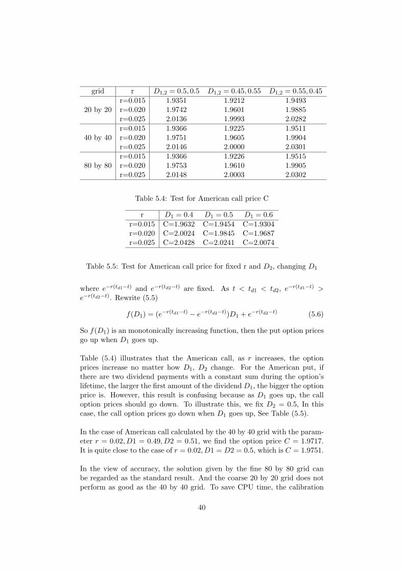
To illustrate how two dividends D1, D2 influence the option price with risk-free interest rate, we put E = 22, td1 = 0.25, td2 = 0.75, σ = 0.25 and T = 1,and change D1, D2 simultaneously with different r. Let D = D1 + D2 = 1.Table (5.3) illustrates that the American put, as r increases, the option pricesdecrease no matter how D1, D2 change. As D = D1 + D2 holds constant,D1 and D2 behave reversely. When td1 and td2 are fixed, the option pricegiven by D1 > D2 is higher than that given by D1 < D2. When applying(5.4), put our attention to D1e

−r(td1−t) + D2e−r(td2−t), we define a function

of D1 asf(D1) = D1e

−r(td1−t) + (1−D1)e−r(td2−t) (5.5)

39

grid r D1,2 = 0.5, 0.5 D1,2 = 0.45, 0.55 D1,2 = 0.55, 0.45

20 by 20r=0.015 1.9351 1.9212 1.9493r=0.020 1.9742 1.9601 1.9885r=0.025 2.0136 1.9993 2.0282

40 by 40r=0.015 1.9366 1.9225 1.9511r=0.020 1.9751 1.9605 1.9904r=0.025 2.0146 2.0000 2.0301

80 by 80r=0.015 1.9366 1.9226 1.9515r=0.020 1.9753 1.9610 1.9905r=0.025 2.0148 2.0003 2.0302

Table 5.4: Test for American call price C

r D1 = 0.4 D1 = 0.5 D1 = 0.6r=0.015 C=1.9632 C=1.9454 C=1.9304r=0.020 C=2.0024 C=1.9845 C=1.9687r=0.025 C=2.0428 C=2.0241 C=2.0074

Table 5.5: Test for American call price for fixed r and D2, changing D1

where e−r(td1−t) and e−r(td2−t) are fixed. As t < td1 < td2, e−r(td1−t) >e−r(td2−t). Rewrite (5.5)

f(D1) = (e−r(td1−t) − e−r(td2−t))D1 + e−r(td2−t) (5.6)

So f(D1) is an monotonically increasing function, then the put option pricesgo up when D1 goes up.

Table (5.4) illustrates that the American call, as r increases, the optionprices increase no matter how D1, D2 change. For the American put, ifthere are two dividend payments with a constant sum during the option’slifetime, the larger the first amount of the dividend D1, the bigger the optionprice is. However, this result is confusing because as D1 goes up, the calloption prices should go down. To illustrate this, we fix D2 = 0.5, In thiscase, the call option prices go down when D1 goes up, See Table (5.5).

In the case of American call calculated by the 40 by 40 grid with the param-eter r = 0.02, D1 = 0.49, D2 = 0.51, we find the option price C = 1.9717.It is quite close to the case of r = 0.02, D1 = D2 = 0.5, which is C = 1.9751.

In the view of accuracy, the solution given by the fine 80 by 80 grid canbe regarded as the standard result. And the coarse 20 by 20 grid does notperform as good as the 40 by 40 grid. To save CPU time, the calibration

40

Grid 20 by 20 40 by 40 80 by 80r=0.015; P=2.5006 P=2.5044 P=2.5051r=0.020; P=2.4490 P=2.4523 P=2.4531r=0.025; P=2.3992 P=2.4020 P=2.4026r=0.015; C=1.9035 C=1.9621 C=1.9057r=0.020; C=1.9411 C=1.9425 C=1.9427r=0.025; C=1.9789 C=1.9057 C=1.9802

Table 5.6: Test for American option for fixed D=1, changing r with volatilitycorrection (2.33), where C for call option price, P for put option price

methods introduced in chapter 6 will apply the 40 by 40 grid to balance theperformance and the accuracy.

5.3 Effect of the parameters using volatility ad-justment

5.3.1 Effect of single dividend and interest rate using volatil-ity adjustment

During the life time of the option we have a single dividend payment D attd. Due to the absence of arbitrage:

S(t+d ) = S(t−d )−D (5.7)

where t+d and t−d are the instants immediately before and after the ex-dividend date. The value V of the option must be smooth as a functionof time over the time of payment

V (S(t+d ), t+d ) = V (S(t−d ), t−d ) (5.8)

We distinguish the following approaches to include a discrete dividend.

The volatility correction (2.33) is volatility correction after td and (2.34)is volatility correction before td which are both applied in the following re-sults. The result given by (2.33) see Tables (5.6), (5.7). The result given by(2.34) see Tables (5.8), (5.9).

Both the volatility correction models behave similarly to the classicalWilmott’s model. The volatility correction method before td provides thelargest option values while the volatility correction method after td providesthe smallest values, and Wilmott’s model gives the results which are almostthe average of the former two.

41


Table 5.7: Test for American option for fixed r=0.02, changing D withvolatility correction (2.33), where C for call option price, P for put optionprice

Grid 20 by 20 40 by 40 80 by 80r=0.015; P=2.5977 P=2.6015 P=2.6021r=0.020; P=2.5450 P=2.5490 P=2.5497r=0.025; P=2.4948 P=2.4980 P=2.4989r=0.015; C=1.9995 C=2.0002 C=2.0007r=0.020; C=2.0364 C=2.0367 C=2.0375r=0.025; C=2.0737 C=2.0747 C=2.0751

Table 5.8: Test for American option for fixed D=1, changing r with volatilitycorrection (2.34), where C for call option price, P for put option price


Table 5.9: Test for American option for fixed r=0.02, changing D withvolatility correction (2.34), where C for call option price, P for put optionprice

42

grid r D1,2 = 0.5, 0.5 D1,2 = 0.45, 0.55 D1,2 = 0.55, 0.45

20 by 20r=0.015 P=2.5048 P=2.5038 P=2.5058r=0.020 P=2.4478 P=2.4469 P=2.4488r=0.025 P=2.3921 P=2.3912 P=2.3930

40 by 40r=0.015 P=2.5078 P=2.5067 P=2.5088r=0.020 P=2.4512 P=2.4501 P=2.4522r=0.025 P=2.3957 P=2.3947 P=2.3966

80 by 80r=0.015 P=2.5086 P=2.5075 P=2.5096r=0.020 P=2.4518 P=2.4508 P=2.4529r=0.025 P=2.3963 P=2.3954 P=2.3973

Table 5.10: Test for American put with volatility correction (2.33)

grid r D1,2 = 0.5, 0.5 D1,2 = 0.45, 0.55 D1,2 = 0.55, 0.45

20 by 20r=0.015 C=1.8938 C=1.8815 C=1.9087r=0.020 C=1.9326 C=1.9201 C=1.9477r=0.025 C=1.9729 C=1.9604 C=1.9871

40 by 40r=0.015 C=1.8970 C=1.8846 C=1.9110r=0.020 C=1.9358 C=1.9231 C=1.9499r=0.025 C=1.9755 C=1.9627 C=1.9896

80 by 80r=0.015 C=1.8976 C=1.8851 C=1.9112r=0.020 C=1.9363 C=1.9235 C=1.9503r=0.025 C=1.9761 C=1.9629 C=1.9902

Table 5.11: Test for American call with volatility correction (2.33)

5.3.2 Effect of two dividends and interest rate using volatil-ity correction

The situation of two discrete dividends model using volatility correction issimilar to the non-volatility correction model. So we just put the resultshere. The result given by (2.33) see Table (5.10) and (5.11). The resultgiven by (2.34) see Table (5.12) and (5.13).

Although the interest rate and the dividend are not the primary factorsaffecting an option’s price, the option trader should still be aware of theireffects. In fact, the primary drawback we have seen in many of the optionanalysis tools available is that they use a simple Black Scholes model whichcan only give the analytical solution to the European style options. Whilein the real market, the options traded are usually American style options.It is better to derive much accurate tools to model the American options bychecking the possibility of early exercise.

43

grid r D1,2 = 0.5, 0.5 D1,2 = 0.45, 0.55 D1,2 = 0.55, 0.45

20 by 20r=0.015 P=2.5538 P=2.5504 P=2.5571r=0.020 P=2.4965 P=2.4933 P=2.4998r=0.025 P=2.4409 P=2.4377 P=2.4441

40 by 40r=0.015 P=2.5565 P=2.5531 P=2.5599r=0.020 P=2.4998 P=2.4965 P=2.5031r=0.025 P=2.4443 P=2.4411 P=2.4475

80 by 80r=0.015 P=2.5573 P=2.5539 P=2.5607r=0.020 P=2.5006 P=2.4973 P=2.5039r=0.025 P=2.4449 P=2.4417 P=2.4482

Table 5.12: Test for American put with volatility correction (2.34)

grid r D1,2 = 0.5, 0.5 D1,2 = 0.45, 0.55 D1,2 = 0.55, 0.45

20 by 20r=0.015 C=1.9420 C=1.9277 C=1.9591r=0.020 C=1.9816 C=1.9670 C=1.9979r=0.025 C=2.0219 C=2.0071 C=2.0370

40 by 40r=0.015 C=1.9454 C=1.9308 C=1.9614r=0.020 C=1.9845 C=1.9696 C=2.0001r=0.025 C=2.0241 C=2.0089 C=2.0400

80 by 80r=0.015 C=1.9460 C=1.9313 C=1.9617r=0.020 C=1.9849 C=1.9698 C=2.0008r=0.025 C=2.0245 C=2.0092 C=2.0406

Table 5.13: Test for American call with volatility correction (2.34)

44

Chapter 6

Calibration of the ImpliedVariables

We use the data of the ING Groep NV to calibrate the implied interest rate,implied dividend and implied volatility. And the data from Fortis Bank willbe used to test the calibration approach. The data is in given the form ofthe following format for one time point in a specific day:

22.140Strike price CallBid CallAsk PutBid PutAsk

15.000 7.150 7.250 0.000 0.05016.000 6.150 6.300 0.000 0.10017.000 5.200 5.300 0.050 0.10018.000 4.200 4.300 0.100 0.15019.000 3.250 3.350 0.150 0.25020.000 2.400 2.450 0.300 0.40021.000 1.550 1.650 0.550 0.65022.000 0.900 0.950 0.950 1.05023.000 0.450 0.500 1.550 1.65024.000 0.150 0.250 2.350 2.45025.000 0.050 0.150 3.250 3.350

Table 6.1: Data of ING on 03-Feb-2005

In Table (6.1), the value 22.140 is the asset closing price at 03-Feb-2005.The values of the first column from 15.000 to 25.000 are the strike prices.The second column is the call option price for bid, the third column is thecall option price for ask, the fourth column is the put option price for bidand the last column is the put option price for ask.

45

To do the calibration, we use two approaches supplied by Matlab. Oneis fminsearch, the other one is fmincon. Both of these methods will bediscussed in the following sections.

6.1 Implied volatility and implied dividend

Implied volatility is a theoretical value designed to represent the volatilityof the security underlying an option as determined by the price of the option.In general, implied volatility decreases when the market is bullish (meanspeople have an optimistic outlook for the market) and increases when themarket is bearish (means people have a pessimistic outlook for the market).This is due to the common belief that bearish markets are more risky thanbullish markets. Implied volatilities are often referred to as a ”market con-sensus”, which is an indication of risk that combines the insights of manymarket participants. However, implied volatilities are essentially parame-ters. They can be biased for some instances. The factors that affect impliedvolatility are the exercise price, the risk-free interest rate, the expiry date,the asset price and the price of the option.

Paying dividend is the one of most important ways of the business to fulfillthe mission of creating profit for the owners. When a company earns a profit,some of this money is typically reinvested in the business and called retainedearnings, and some of it can be paid to its shareholders as a dividend. Theamount of the dividend is determined every year at the company’s annualgeneral meeting, and declared as either a cash amount or a percentage ofthe company’s profit. When a share is sold shortly before the dividend is tobe paid, the seller rather than the buyer is entitled to the dividend. At thepoint at which the buyer is not entitled to the dividend if the share is sold,the share is said to go ex-dividend. This is usually two business days beforethe dividend is to be paid, depending on the rules of the stock exchange.When a share goes ex-dividend, its price will generally fall by the amountof the dividend. Implied dividend in this paper is the market expectationof the dividend, which we want to test if it is close to the dividend havingbeen announced by the company.

In the option pricing formulas, such as the Black Scholes formula, the onlyunknown parameter is the implied volatility of the underlying stock. Ourpurpose in option pricing is to find the implied volatility, given the observedprice quoted in the market. For example, given C0, a price of a call option,the following equation should be solved for the value of σ:

C0 = CBS(S,E, r, σ, T ) (6.1)

46

Actually, it is an inverse problem to solve σ in (6.1), and this equation hasno closed form solution, which means the equation need to be numericallysolved.

If there is a dividend payment during the option’s lifetime, we can use anadjusted form of (6.1):

C0 = CBS(S −D,E, r, σS

S −D,T ) (6.2)

C0 = CBS(S − e−rtdD,E, r, σS

S − e−rtdD,T ) (6.3)

Adjustments (6.2) and (6.3) are similar, and the only difference is that (6.3)uses a discounted dividend D instead of D itself.

In this case, the unknown variables are both D and σ, and not only σmentioned in (6.1), because we assume the dividend payment is also impliedin the real market. So an optimization method has been derived to solvethe two unknown variables problem:

min(σ,D)

N∑

i=1

|Cmarket − C(S, Ei, T, td, (σimp, Dimp))|2 (6.4)

Formula (6.4) is minimized to find the most suitable (σ,D) in our analyticalmodel to fit the market option price.

6.2 Calibration Methods

I. fminsearchfminsearch finds the minimum of a scalar function of several variables, start-ing at an initial estimate. This is generally referred to as unconstrainednonlinear optimization. To do this, using x = fminsearch(fun, x0), whichstarts at the initial point x0 and finds a local minimum x of the functiondescribed in fun.

fminsearch uses the simplex search method named the Nelder-Mead algo-rithm [2]. Four scalar parameters must be specified to define a completeNelder-Mead method: coefficients of reflection ρ, expansion χ, contractionγ, and shrinkage σ. According to the original Nelder-Mead paper, theseparameters should satisfy

ρ > 0, χ > 1, χ > ρ, 0 < γ < 1 and 0 < σ < 1

At the beginning of the kth iteration, k ≥ 0, a nondegenerate simplex (a

47

geometrical figure consisting of N +1 vertices in N dimensions, whereas theN + 1 vertices span a N -dimensional vector space) ∆k is given, along withits n + 1 vertices, each of which is a point in Rn. It is always assumed thatiteration k begins by ordering and labelling these vertices as x

(k)1 , ..., x

(k)n+1,

such thatf

(k)1 ≤ f

(k)2 ≤ ... ≤ f

(k)n+1

Where f(k)i denotes f(x(k)

i ). The kth iteration generates a set of n+1 verticesthat define a different simplex for the next iteration, so that ∆k+1 6= ∆k.Because we seek to minimize f , we refer to x

(k)1 as the best point, to x

(k)n+1

as the worst point. Similarly, we refer to f(k)n+1 as the worst function value,

and so on.

One iteration of the Nelder-Mead algorithm:

1. Order. Order the n+1 vertices to satisfy f(x1) ≤ f(x2) ≤ ... ≤ f(xn+1),using the tie-breaking rules given below.

2. Reflection. Compute the reflection point xr from

xr = x + ρ(x− xn + 1) = (1 + ρ)x− ρxn+1

where x = (1/n)∑n

i=1 xi is the centroid of the n best points (all points ex-cept for xn+1).Evaluate fr = f(xr), if f1 ≤ fr < fn, accept the reflected point xr andterminate the iteration.

3. Expand. If fr < f1, calculate the expansion point xe,

xe = x + χ(xr − x) = x + ρχ(x− xn+1) = (1 + ρχ)x− ρχxn+1

and evaluate fe = f(xe). If fe < fr, accept xe and terminate the iteration;if fe ≥ fr, accept xr and terminate the iteration.

4.Contract. If fr ≥ fn, perform a contraction between x and the bet-ter of xn+1 and xr.

a.Outside. If fn ≤ fr < fn + 1, perform an outside contraction: calculate

xc = x + γ(xr − x) = x + γρ(x− xn+1) = (1 + ργ)x− ργxn+1

Evaluate fc = f(xc). If fc ≤ fr, accept xc and terminate the iteration;otherwise, go to step 5.b.Inside. If fr ≥ fn+1, perform an inside contraction:

xcc = x− γ(x− xn+1) = (1− γ)x + γxn+1

48

Evaluate fcc = f(xcc). If fcc < fn+1, accept xcc and terminate the iteration;otherwise go to step 5.

5. Perform a shrink step. Evaluate f at the n points vi = x1+σ(xi−x1),i = 2, 3, ..., n + 1. The (unordered) vertices of the simplex at the next itera-tion consist of x1, v2, ..., vn + 1.

The limitation is that fminsearch can only give local solutions, and fmin-search is a quite slow algorithm.

II. fiminconfmincon attempts to find a constrained minimum of a scalar function ofseveral variables starting at an initial estimate. This is generally referredto as constrained nonlinear optimization or nonlinear programming. Inx = fmincon(fun, x0, A, b, Aeq, beq, lb, ub), fun is the objective function,x0 is the starting point. A, b present the constrained linear inequalitiesAx ≤ b. Aeq, beq present the constrained linear equalities Aeq · x = beq.And lb, ub give the lower and upper bounds of x, respectively.

In our situation, the medium-scale algorithm of fmincon is used, which usesthe sequential quadratic programming (SQP) method with BFGS method[3].

The SQP implementation consists of three main stage:

1. Updating the Hessian MatrixAt each major iteration a positive definite quasi-Newton approximation ofthe Hessian of the Lagrangian function, H, is calculated using the BFGSmethod, where λi(i = 1, ..., m) is an estimate of the Lagrange multipliers.

Hk+1 = Hk +qkq

Tk

qTk sk

− HTk Hk

sTk Hksk

where

sk = xk+1 − xk

qk = ∇f(xk+1) +n∑

i=1

λi∇gi(xk+1)− (∇f(xk) +n∑

i=1

λi∇gi(xk))

2.Quadratic Programming SolutionAt each major iteration of the SQP method, a QP problem of the followingform is solved

minimize q(d) =12dT Hd + cT d

Aid = bi i = 1, ...,me

Aid ≤ bi i = me + 1, ..., m

49

3.Line Search and Merit FunctionThe solution to the QP subproblem produces a vector dk, which is used toform a new iterate

xk+1 = xk + αkdk

The step length parameter αk is determined in order to produce a sufficientdecrease in a merit function, given by the following implementation.

Ψ(x) = f(x) +me∑

i=1

rigi(x) +m∑

i=me+1

rimax(0, gi(x))

In our model, only the upper and lower bounds of the variables are de-fined, such that implied interest rate 0.01 ≤ r ≤ 1, implied dividend0.01 ≤ D ≤ S0 and implied volatility 0.01 ≤ σ ≤ 0.5.

6.3 Comparison of fmincon and fminsearch

Compare the results derived by fminsearch and fmincon by taking the ex-ample of Table (6.1):

fminsearchr D0.01886 0.89670sigma0.25688 0.21438 0.18943 0.18019 0.17082 0.16451 0.15506 0.15633error0.00016

Table 6.2: Test for fminsearch

fminconr D0.01883 0.89621sigma0.25650 0.21434 0.18944 0.18018 0.17079 0.16451 0.15507 0.15631error0.00016

Table 6.3: Test for fmincon

50

The CPU time for the fminsearch is 1442.648s and for fmincon is 232.664s,and the calibrated results of these two methods are nearly the same. Giventhe similar results, fmincon performs much faster than fminsearch. So wechoose fmincon as our main optimization approach.

6.4 Algorithm of the whole approach

The algorithm of the whole approach can be described by the picture below.Firstly, the program reads the all of the data from the directory; then weset the initial guess of the parameters which need to be calibrated; afterthat we use Black-Scholes equation to calculate the option price given theinitial parameters; finally, fmincon is used to find the optimal solution of theparameters in such a way that if the value of the objective function (in thiscase it is the difference between the calibrated option prices and the marketprices) is larger than a certain constant (in our case it is 10−6), fmincon willupdate the initial parameters. The updated parameters will be set as theinitial parameters and put into the algorithm to produce another value ofthe objective function and so on.

Figure 6.1: Algorithm of the whole approach

51

6.5 Objective Functions

The basic objective function we use is the Sum of Relative Error (SRE):

MSE =n∑

i=1

[Cicalib − Ci

market]2

Cimarket

+n∑

i=1

[P icalib − P i

market]2

P imarket

(6.5)

Where Cmarket = (CallAsk+CallBid)/2 and Pmarket = (PutAsk+PutBid)/2.Take the third row in Table (6.1) for example, where the strike price E = 20,and CallBid = 2.600, CallAsk = 2.700, PutBid = 0.850 and PutAsk =0.950.Traders who make markets routinely quote two prices, one to buy(bid) and one to sell (ask), where his selling price is always higher than hisbuying price. This difference is known as the Bid-Ask spread. Essentially,the dealer is offering a put to sell to him at his bid price and a call to buyfrom him at his ask price. The price he charges for these two options is theBid-Ask spread.

According to the bid-ask spread, we add some extra features to the ob-jective function. In more detail, if the calibrated option price falls into theinterval of [Bid,Ask], we put a weight µ ∈ (0, 1) in front of [Ci

calib−Cimarket]

2

Cimarket

and [P icalib−P i

market]2

P imarket

.

This objective function (6.5) does not perform very well when the calibratedoption price may lay outside the interval of [Bid,Ask]. Because it is only us-ing the average of Ask and Bid, while in the real market, the option price issometimes close to Ask and sometimes close to Bid but outside the interval.An example will be illustrated later. So we derive another objective functionto deal with the situation that the calibrated option prices lay outside theinterval of [Bid,Ask]:

MSE =n∑

i=1

CiMSE +

n∑

i=1

P iMSE (6.6)

where

CiMSE =

[Cicalib − CallBidi]2

Cimarket

Cicalib < CallBid

[Cicalib − CallAski]2

Cimarket

Cicalib > CallAsk

µ[Ci

calib − Cimarket]

2

Cimarket

Cicalib ∈ [CallBid, CallAsk]

(6.7)

52

P iMSE =

[P icalib − PutBidi]2

P imarket

P icalib < PutBid

[P icalib − PutAski]2

P imarket

P icalib < PutAsk

µ[P i

calib − P imarket]

2

P imarket

P icalib ∈ [PutBid, PutAsk]

(6.8)

6.6 Calibration Results

6.6.1 Single dividend from ING

We first examine the single dividend case, and aim to deduce from the datawhen the dividend is announced and how the dividend amount of the INGbehaves in 2005. The option data has been collected day by day, startingfrom 22-Jan-2005, and in this test the options expire on 17-Jun-2005. Thedate string 22-Jan-2005 can be transformed to the number 38373 by Matlab.

As we have already know that the ING Groep pays the dividend twice ayear, in 2005 on 28-Apr-2005 and 12-Aug-2005. The dividend are e0.58 ande0.49, respectly. The dividend announcement date is 17-Feb-2005.

There are some aims we want to achieve:

• The first implied dividend amount after 17-Feb-2005 should be around0.58

• The dividend announcement date should be made visible, if the markethad a different guess of the size of the dividend

• The errors in the optimization should be reasonably small

• The calibrated results should be stable over several days

In the first test, all of the parameters are calibrated simultaneously. The re-sults are in Table (6.4), where Sigma15 is according to the implied volatilityfor the strike price 15. The calibrated risk-free interest rate is around 0.02,while the interest rate given by the European Central Bank is also around0.02 in the first six months in 2005. To simplify the problem and to avoidmultiple optimal solutions with unstable parameters among r and D, therisk-free interest rate r will be fixed at 0.02 in later calculations.

Using the objective function with (6.5), we obtain the results in Table(6.5). The implied dividend amount, one of the implied volatilities and theerrors are given with the initial date, the expiry date and the fixed risk-freeinterest rate. It is obvious that there is a jump in the dividend amount at

53

Initial date Expiry date Interest rate Dividend Sigma15 Error38373 38527 0.021939 0.515946 0.296387 0.00015538376 38527 0.020103 0.490714 0.307422 0.00036438377 38527 0.020962 0.493104 0.279730 0.00008538378 38527 0.021357 0.505352 0.276019 0.00034138379 38527 0.021553 0.512003 0.305813 0.00019738380 38527 0.018829 0.439513 0.276437 0.00006338383 38527 0.025857 0.515767 0.281370 0.00008138384 38527 0.021164 0.507776 0.318473 0.00049638385 38527 0.018968 0.499693 0.286197 0.00011538386 38527 0.023126 0.497379 0.287140 0.00027838387 38527 0.022551 0.511048 0.292522 0.00037738390 38527 0.020036 0.511128 0.300797 0.00031838392 38527 0.021459 0.533613 0.298096 0.00027538393 38527 0.022667 0.508263 0.298962 0.00045638394 38527 0.020933 0.487833 0.312863 0.00015638397 38527 0.022944 0.506561 0.318011 0.00014338398 38527 0.019561 0.487557 0.322057 0.00022138399 38527 0.018607 0.467708 0.318818 0.00012538400 38527 0.020575 0.558542 0.324225 0.00027338401 38527 0.021078 0.583934 0.322581 0.00038138404 38527 0.022588 0.574570 0.324551 0.00078438405 38527 0.021921 0.584837 0.320452 0.00039638406 38527 0.022080 0.575445 0.320655 0.000303

Table 6.4: ING option with all parameters calibrated

38399 of the initial date, which is 17-Feb-2005. Before 17-Feb-2005, the div-idend amount is around 0.50 which is the dividend amount paid by ING in2004, while after 17-Feb-2005, the dividend amount moves around 0.58. Theerrors are always less than 0.01, so the calibrated results can be accepted.And the results can be thought stable in some sense.

Table 6.5: ING option with fixed interest rate

Initial date Expiry date Interest rate Dividend Sigma15 Error38373 38527 0.02 0.508066 0.294281 0.00013238376 38527 0.02 0.499899 0.305448 0.00038238377 38527 0.02 0.493971 0.277986 0.00009538378 38527 0.02 0.502031 0.274090 0.00033238379 38527 0.02 0.508028 0.303789 0.00017738380 38527 0.02 0.509099 0.273610 0.000598

54

38383 38527 0.02 0.470633 0.279811 0.00016238384 38527 0.02 0.507680 0.316680 0.00052838385 38527 0.02 0.521320 0.284080 0.00020938386 38527 0.02 0.478650 0.285420 0.00027338387 38527 0.02 0.499800 0.290870 0.00038738390 38527 0.02 0.478660 0.299560 0.00031038392 38527 0.02 0.489680 0.296750 0.00034738393 38527 0.02 0.471200 0.297490 0.00049038394 38527 0.02 0.492670 0.310990 0.00015638397 38527 0.02 0.493430 0.316120 0.00014638398 38527 0.02 0.504317 0.319456 0.00027438399 38527 0.02 0.508441 0.316489 0.00044038400 38527 0.02 0.571386 0.321308 0.00029338401 38527 0.02 0.551329 0.320453 0.00044838404 38527 0.02 0.572366 0.322161 0.00099438405 38527 0.02 0.574956 0.318423 0.00028438406 38527 0.02 0.579970 0.318630 0.00036438407 38527 0.02 0.608180 0.318177 0.00073438408 38527 0.02 0.567505 0.332179 0.00021338411 38527 0.02 0.602965 0.344433 0.00127538412 38527 0.02 0.593130 0.350710 0.00045438413 38527 0.02 0.565210 0.356530 0.00024838414 38527 0.02 0.573970 0.362660 0.00010938415 38527 0.02 0.583940 0.370070 0.00067238418 38527 0.02 0.562920 0.378490 0.00156738419 38527 0.02 0.562630 0.373690 0.00051738420 38527 0.02 0.588990 0.375460 0.00051838421 38527 0.02 0.576980 0.367810 0.00063738422 38527 0.02 0.543080 0.370860 0.00028938427 38527 0.02 0.570239 0.371011 0.00025838428 38527 0.02 0.576388 0.369521 0.00044038429 38527 0.02 0.586651 0.376288 0.00076038432 38527 0.02 0.568003 0.383667 0.00053438433 38527 0.02 0.575822 0.378273 0.00058838434 38527 0.02 0.578276 0.380609 0.00048238435 38527 0.02 0.577024 0.393358 0.00074838436 38527 0.02 0.572623 0.396551 0.00064938439 38527 0.02 0.564013 0.403160 0.00049738440 38527 0.02 0.597608 0.404688 0.00147038441 38527 0.02 0.587600 0.402521 0.00068538442 38527 0.02 0.607204 0.404909 0.00181338443 38527 0.02 0.576860 0.405670 0.00044238446 38527 0.02 0.559460 0.403110 0.00035738447 38527 0.02 0.573040 0.402880 0.000479

55

38448 38527 0.02 0.567140 0.411290 0.00079238449 38527 0.02 0.584720 0.424580 0.00041738450 38527 0.02 0.569100 0.423700 0.00037338454 38527 0.02 0.593440 0.425780 0.00123738455 38527 0.02 0.596220 0.437540 0.00056838457 38527 0.02 0.582936 0.432096 0.00046438460 38527 0.02 0.595361 0.406600 0.00114538461 38527 0.02 0.606763 0.393427 0.00246338462 38527 0.02 0.570960 0.395335 0.00065338463 38527 0.02 0.612593 0.401268 0.00046938464 38527 0.02 0.588554 0.415965 0.00039738467 38527 0.02 0.560588 0.436865 0.00072838469 38527 0.02 0.573752 0.410784 0.001139

However, using the objective function with (6.5), the implied volatility be-comes larger and larger when the option is close to its maturity, which canbe shown in the Table (6.6).

As we all know that the implied volatility cannot go beyond 1 in the

Initial date Expiry date Interest rate Sigma15 Sigma25 Error38492 38527 0.02 0.624756 0.239844 0.00175038495 38527 0.02 0.629482 0.263826 0.00132638496 38527 0.02 0.623689 0.269366 0.00101338497 38527 0.02 0.652232 0.262197 0.00104438498 38527 0.02 0.678379 0.256337 0.00108638499 38527 0.02 0.695198 0.261571 0.00071138509 38527 0.02 0.844717 0.327253 0.00773138510 38527 0.02 0.864703 0.296577 0.00872538511 38527 0.02 0.893884 0.313207 0.00165038512 38527 0.02 0.936581 0.316499 0.00188038513 38527 0.02 0.979555 0.328685 0.01042138516 38527 0.02 1.080919 0.366025 0.00917838517 38527 0.02 1.075210 0.374596 0.02210238518 38527 0.02 1.145459 0.389684 0.02878138519 38527 0.02 1.240903 0.396630 0.05045938520 38527 0.02 1.355987 0.414168 0.110484

Table 6.6: ING option close to maturity with the objective function (6.5)

real market, so the calibrated implied volatility is clearly too high. The

56

calibrated implied volatility which is according to the strike price 15 is in-creasing to 1.355987. Take the data of the day 38520 for example, see Table(6.7):


15.000 8.200 8.300 0.000 0.05016.000 7.200 7.300 0.000 0.05017.000 6.200 6.300 0.000 0.05018.000 5.200 5.250 0.000 0.05019.000 4.200 4.300 0.000 0.05020.000 3.200 3.250 0.000 0.05021.000 2.200 2.250 0.000 0.05022.000 1.200 1.250 0.000 0.05023.000 0.200 0.250 0.050 0.05024.000 0.000 0.050 0.700 0.80025.000 0.000 0.050 1.700 1.800

Table 6.7: Data of ING on 17-Jun-2005

We can see that when the option is close to its maturity, only as the strikeprices are around the asset price, the option price for bid is not zero. Thereason is simple, the market assumes that the asset price cannot move toohigh or too low in a few days, so the option cannot be exercised when thestrike prices are far away from the asset price. When the strike price is 15,the option put price is close to 0, while the strike price is 22, the option putprice will be close to 0.05. So applying the objective function with (6.5),we cannot calibrate the option price very well, since it is only calculate theaverage of Bid and Ask. To improve the results, the objective function (6.6)will be used, and the results are presented in Table (6.8):

Using the objective function (6.6), the calibrated implied volatility ac-cording to the strike price 15 becomes quite stable around 0.4. However,the calibrated implied volatility according to the strike price 25 is not yetstable, for sometimes it reaches the lower bound 0.05 of the fmincon opti-mization method, and at this time, the some errors are larger than 0.01.

To avoid the situation that calibrated parameters reach their lower or up-per bound, we set the calibrated parameters p0(t) of data(t) as the initialguess of date(t+1). We set p0(t)− bI as the lower bound for date(t+1) andp0(t)+bI as the upper bound for date (t), where b is a small value dependingon how the parameters behave and I is the vector with all elements equal

57

Initial date Expiry date Interest rate Sigma15 Sigma25 Error38492 38527 0.02 0.400001 0.160288 0.00004238495 38527 0.02 0.399997 0.050000 0.01001438496 38527 0.02 0.400001 0.050000 0.01001038497 38527 0.02 0.400000 0.050000 0.01365138498 38527 0.02 0.400004 0.171814 0.00001138499 38527 0.02 0.399994 0.195138 0.00000938509 38527 0.02 0.400000 0.050000 0.00425638510 38527 0.02 0.399999 0.050000 0.01078338511 38527 0.02 0.400000 0.256493 0.00011138512 38527 0.02 0.400000 0.050003 0.01006438513 38527 0.02 0.399999 0.050029 0.01006738516 38527 0.02 0.399999 0.276694 0.00011538517 38527 0.02 0.400000 0.282023 0.00012038518 38527 0.02 0.399999 0.296542 0.00006138519 38527 0.02 0.400000 0.310489 0.00021138520 38527 0.02 0.400005 0.330762 0.047473

Table 6.8: ING option close to maturity with the objective function (6.6)

to 1. So the calibrated parameters p0(t + 1) is bounded by a small rangederived by p0(t). With the updated p0, the results become much better,which can be seen in Table (6.6.1):

Using the objective function (6.6) with the updated p0, the calibrated im-plied volatility according to the strike price 15 becomes quite stable around0.41944. The calibrated implied volatility according to the strike price 22does not reach its lower bound any longer. Also the error remaining after theoptimization with objective function (6.6) and updated p0 performs muchbetter than the results given by objective function (6.5) as well as objectivefunction (6.6) without updated p0. The only drawback is that the error ofthe last day is larger than 0.01.

With the updated p0, the CPU time can be saved because the difference be-tween two arbitrary adjacent p0 is small, so fmincon can easily find p0(t+1)given p0(t). How much CPU time can saved with updated p0 depends onthe initial guess of p0 in a time step. In my case, I put the initial guessas p0 = [0.4, 0.38, 0.36, ..., 0.2] for each step. While using the updated p0,the gain in CPU time is 20%-25%. If the initial guess is far away from thecalibrated result, updated p0 can save even more CPU time.

58

The implied volatility can be shown by the pictures as Figure (6.2)-(6.5):

6.6.2 Two dividends from ING

For the ING Groep pays dividend twice in 2005, we calibrate next the sec-ond dividend amount of the ING stock. All options we used here will expireon 16-Dec-2005 (38701). Firstly, both of the first dividend and the seconddividend will be calibrated simultaneously, and the results are put in Ta-ble (6.10). In this table, the dividend announcement date cannot be foundin the column of Dividend 1. And after the dividend announcement date(38399), the first dividend does not move around 0.58, meanwhile the seconddividend does not move around 0.49, although the error performs well. Thisis due to the existence of multiple optimal solutions if both D1 and D2 arechosen as parameters to be optimized.

Therefore we fix the first dividend amount given by Table (6.5), and weonly calibrate the second dividend amount and the implied volatilities. Thistime the amount of the second dividend goes round 0.49 with the error alsoperforming well. The results are presented in Table (6.11).

Initial date Expiry date Interest rate Sigma15 Sigma25 Error38492 38527 0.02 0.41944 0.24428 1.67E-0538495 38527 0.02 0.41944 0.26386 6.98E-0638496 38527 0.02 0.41944 0.26936 0.00011338497 38527 0.02 0.41944 0.26215 4.64E-0638498 38527 0.02 0.41945 0.25653 1.26E-0538499 38527 0.02 0.41945 0.26158 9.80E-0638509 38527 0.02 0.41945 0.32742 0.00071738510 38527 0.02 0.41945 0.29669 0.00069338511 38527 0.02 0.41945 0.31324 7.31E-0638512 38527 0.02 0.41945 0.31652 1.23E-0538513 38527 0.02 0.41945 0.32905 9.85E-0538516 38527 0.02 0.41945 0.35405 9.70E-0538517 38527 0.02 0.41945 0.35869 9.25E-0538518 38527 0.02 0.41945 0.37623 4.38E-0538519 38527 0.02 0.41945 0.39153 0.00012638520 38527 0.02 0.41945 0.41505 0.046697

Table 6.9: ING option close to maturity with the objective function (6.6)and updated p0

59

15 16 17 18 19 20 21 22 23 24 25

0.16

0.18

0.2

0.22

0.24

0.26

0.28

0.3Implied volatility of 21−Jan−2005

Figure 6.2: Implied volatility of ING on 21-Jan-2005

15 16 17 18 19 20 21 22 23 24 25

0.2

0.25

0.3

0.35

0.4

0.45

0.5Implied volatility of 28−Apr−2005

Figure 6.3: Implied volatility of ING on 28-Apr-2005

60

15 16 17 18 19 20 21 22 23 24 25

0.2

0.25

0.3

0.35

0.4

0.45

0.5Implied volatility of 29−Apr−2005

Figure 6.4: Implied volatility of ING on 29-Apr-2005

15 16 17 18 19 20 21 22 23 24 250.1

0.15

0.2

0.25

0.3

0.35

0.4

0.45

0.5Implied volatility of 17−Jun−2005

Figure 6.5: Implied volatility of ING on 17-Jun-2005

61

Initial date Expiry date Dividend 1 Dividend 2 Error38373 38701 0.482873 0.480260 0.00001738376 38701 0.474995 0.484836 0.00016138377 38701 0.475825 0.516397 0.00013638378 38701 0.468500 0.488297 0.00050538379 38701 0.476493 0.515834 0.00043138380 38701 0.507224 0.497765 0.00044138383 38701 0.472092 0.476802 0.00023638384 38701 0.432050 0.534076 0.00005938385 38701 0.499337 0.500311 0.00016838386 38701 0.431131 0.522670 0.00026438387 38701 0.446490 0.508677 0.00022738390 38701 0.477264 0.481752 0.00027738392 38701 0.463684 0.496962 0.00028138393 38701 0.459182 0.484533 0.00044238394 38701 0.441031 0.541017 0.00005938397 38701 0.443271 0.527188 0.00031838398 38701 0.441893 0.546166 0.00026338399 38701 0.461823 0.525720 0.00022138400 38701 0.449991 0.610474 0.00018238401 38701 0.444835 0.598729 0.00022038404 38701 0.514305 0.564121 0.00021438405 38701 0.499460 0.571135 0.00027038406 38701 0.503694 0.573947 0.000252

Table 6.10: ING option with two dividends calibrated simultaneously

62

Initial date Expiry date Dividend 1 Dividend 2 Error38373 38701 0.508066 0.459462 0.00004838376 38701 0.499899 0.464669 0.00013338377 38701 0.493971 0.506920 0.00015838378 38701 0.502031 0.457849 0.00038438379 38701 0.508028 0.490483 0.00036838380 38701 0.509099 0.498679 0.00031638383 38701 0.470633 0.484704 0.00022138384 38701 0.507680 0.468061 0.00005138385 38701 0.521320 0.479604 0.00010838386 38701 0.478650 0.484413 0.00022638387 38701 0.499800 0.459513 0.00012138390 38701 0.478660 0.484386 0.00016838392 38701 0.489680 0.476040 0.00024538393 38701 0.471200 0.479320 0.00036538394 38701 0.492670 0.503361 0.00006238397 38701 0.493430 0.486962 0.00032338398 38701 0.504317 0.499030 0.00027738399 38701 0.508441 0.488948 0.00023938400 38701 0.571386 0.508508 0.00021738401 38701 0.551329 0.511860 0.00027638404 38701 0.572366 0.484170 0.00019838405 38701 0.574956 0.504191 0.00007738406 38701 0.579970 0.510321 0.000267

Table 6.11: ING option the 2nd dividend is calibrated with the 1st dividendfixed

The calibration results given in this section are calculated by the objec-tive function (6.5) without the updated p0. We find that when the option isfar from maturity, the objective function (6.5) performs well. Without theupdated p0, we can investigate how the implied dividend behaves in a muchwider range.

6.6.3 Calibrated parameters for Fortis option

Fortis Bank pays one dividend on 27-May-2005, and the dividend amountis e1.17 with the dividend announcement date 10-Mar-2005 (38420). Theobjective function (6.6) with the updated p0 is applied, the results are shownin Table (6.13). The risk-free interest rate is fixed to 0.02, which is not shownin Table (6.13). And the data from Fortis are presented in Table (6.12).

63


10.000 11.35 11.45 0.000 0.05015.000 6.400 6.500 0.050 0.10016.000 5.400 5.500 0.050 0.10017.000 4.450 4.550 0.100 0.15018.000 3.500 3.550 0.200 0.25019.000 2.550 2.650 0.350 0.45020.000 1.750 1.800 0.650 0.70021.000 1.000 1.100 1.100 1.15022.000 0.500 0.600 1.750 1.85023.000 0.250 0.300 2.550 2.65025.000 0.000 0.100 4.400 4.500

Table 6.12: Data of Fortis on 21-Jan-2005

Table 6.13: Fortis option with fixed interest rate

Initial date Expiry date Dividend Sigma10 Sigma25 Error38373 38527 0.934826 0.479580 0.155082 0.00000338376 38527 0.933933 0.479580 0.158532 0.00000938377 38527 0.906764 0.479583 0.147468 0.00000538378 38527 0.907638 0.479584 0.154727 0.00000838379 38527 0.922589 0.479584 0.157866 0.00000438380 38527 0.942229 0.479585 0.157668 0.00000538383 38527 0.934152 0.479585 0.163426 0.00001038384 38527 0.934003 0.479586 0.170400 0.00000838385 38527 0.933845 0.479586 0.164047 0.00001138386 38527 0.932407 0.479587 0.160272 0.00001038387 38527 0.922614 0.479587 0.158921 0.00000338390 38527 0.925925 0.479587 0.160187 0.00000438392 38527 0.925607 0.479587 0.152542 0.00000338393 38527 0.912323 0.479588 0.151124 0.00001338394 38527 0.952026 0.479588 0.142895 0.00000538397 38527 0.949771 0.479589 0.149649 0.00002338398 38527 0.958215 0.479596 0.139104 0.00000738399 38527 0.957089 0.479597 0.141944 0.00001338400 38527 0.960785 0.479597 0.144045 0.00000638401 38527 0.927932 0.479599 0.142476 0.00000638404 38527 0.939053 0.479599 0.149856 0.00000138405 38527 0.926781 0.479599 0.156725 0.00010438406 38527 0.927193 0.479599 0.165605 0.000002

64

38407 38527 0.926990 0.479599 0.162830 0.00000338408 38527 0.927654 0.479599 0.162117 0.00000938411 38527 0.929799 0.479599 0.158942 0.00001338412 38527 0.930128 0.479599 0.166958 0.00002438413 38527 0.929641 0.479599 0.167150 0.00000238414 38527 0.931700 0.479599 0.165220 0.00000938415 38527 0.964984 0.479599 0.160406 0.00004938418 38527 0.976377 0.479599 0.159571 0.00000438419 38527 1.000629 0.479594 0.154133 0.00000338420 38527 1.011569 0.479594 0.147061 0.00000438421 38527 1.010606 0.479594 0.152109 0.00000538422 38527 1.010516 0.479594 0.154522 0.00000238427 38527 1.009660 0.479594 0.164579 0.00000438428 38527 1.009484 0.479594 0.164527 0.00001038429 38527 1.019464 0.479595 0.149867 0.00000138432 38527 1.033535 0.479594 0.145934 0.00000338433 38527 1.032625 0.479594 0.146997 0.00000538434 38527 1.032301 0.479594 0.158290 0.00000638435 38527 1.030352 0.479593 0.150290 0.00001838436 38527 1.030852 0.479593 0.151442 0.00000438439 38527 1.031113 0.479593 0.154709 0.00000438440 38527 1.081113 0.479591 0.151861 0.00000638441 38527 1.031113 0.479588 0.165305 0.00005038442 38527 1.030962 0.479588 0.161890 0.00000338443 38527 1.030629 0.479588 0.164521 0.00000338446 38527 1.030070 0.479588 0.177992 0.00000238447 38527 1.027633 0.479587 0.171208 0.00000638448 38527 1.021150 0.479586 0.172900 0.00000238449 38527 1.035994 0.479582 0.168697 0.00000238450 38527 1.008158 0.479582 0.163340 0.00000538454 38527 1.008731 0.479581 0.174451 0.00000838455 38527 1.004585 0.479581 0.170320 0.00000338456 38527 1.004665 0.479581 0.177057 0.00000238457 38527 1.005419 0.479581 0.184053 0.00000838460 38527 1.039402 0.479581 0.213607 0.00001138461 38527 1.039944 0.479581 0.214393 0.00000738462 38527 1.039629 0.479581 0.221684 0.00000238463 38527 1.032678 0.479580 0.225774 0.00000238464 38527 1.045315 0.479580 0.224126 0.00000438467 38527 1.062951 0.479580 0.225187 0.00001038469 38527 1.045876 0.479580 0.241575 0.00000538470 38527 1.057039 0.479575 0.250408 0.00010038471 38527 1.057493 0.479575 0.253198 0.00002038474 38527 1.056956 0.479575 0.247895 0.000012

65

38475 38527 1.056514 0.479575 0.248678 0.00000538476 38527 1.042808 0.479575 0.240271 0.00000738477 38527 1.042729 0.479575 0.233832 0.00001138478 38527 1.029811 0.479575 0.234915 0.00000438481 38527 1.028795 0.479574 0.240241 0.00000538482 38527 1.023615 0.479574 0.245488 0.00001338483 38527 1.021258 0.479574 0.255283 0.00000738484 38527 1.031844 0.479574 0.252362 0.00001038485 38527 1.029856 0.479574 0.260979 0.00000438488 38527 1.042315 0.479574 0.268128 0.00002038489 38527 1.042897 0.479574 0.265446 0.00000438490 38527 1.040857 0.479574 0.256947 0.00000538491 38527 1.043940 0.479574 0.243960 0.00001038492 38527 1.068721 0.479574 0.245937 0.00002238495 38527 1.062535 0.479574 0.247910 0.00001138496 38527 1.072398 0.479574 0.250730 0.00003138497 38527 1.052399 0.479574 0.253154 0.00003438498 38527 1.050820 0.479574 0.254159 0.00005338499 38527 0.000000 0.479574 0.246641 0.00001038509 38527 0.000000 0.479574 0.285461 0.00000238510 38527 0.000000 0.479548 0.270867 0.00005738511 38527 0.000000 0.479548 0.280724 0.00003338512 38527 0.000000 0.479548 0.275813 0.00072338513 38527 0.000000 0.479548 0.284427 0.00007138516 38527 0.000000 0.479548 0.307466 0.00000538517 38527 0.000000 0.479548 0.298895 0.00013638518 38527 0.000000 0.479548 0.314530 0.00000638519 38527 0.000000 0.479548 0.320255 0.00010938520 38527 0.000000 0.479548 0.315301 0.010113

In Table (6.13), the implied dividend moves up to 1 on the date (38419)which is one day before the dividend announcement. This situation hap-pening may be resulted from the market having expected that the dividendof Fortis bank will be announced. And the calibrated implied dividend isaround 1.05 which is a little lower than the announcement. The impliedvolatility according to both strike price 15 and 25 both perform quite well.And most of the errors are smaller than 0.01 except the last one.

The implied volatility of Fortis can be shown by the pictures as Figure(6.6)-(6.9):

66

10 15 20 25

0.2

0.25

0.3

0.35

0.4

0.45

0.5Implied volatility of 21−Jan−2005 of Fortis

Figure 6.6: Implied volatility of Fortis on 21-Jan-2005

10 15 20 250.1

0.15

0.2

0.25

0.3

0.35

0.4

0.45

0.5Implied volatility of 26−May−2005 of Fortis

Figure 6.7: Implied volatility of Fortis on 26-May-2005

67

10 15 20 250.1

0.15

0.2

0.25

0.3

0.35

0.4

0.45

0.5Implied volatility of 27−May−2005 of Fortis

Figure 6.8: Implied volatility of Fortis on 27-May-2005

10 15 20 250.05

0.1

0.15

0.2

0.25

0.3

0.35

0.4

0.45

0.5Implied volatility of 17−Jun−2005 of Fortis

Figure 6.9: Implied volatility of Fortis on 17-Jun-2005

68

Chapter 7

Conclusion

The Black-Scholes equation is a useful and fundamental tool to calculate theoption prices. Since the stock options in the real market are all of Ameri-can type, there is no closed form to solve the Black-Scholes equation. In ourcode, the fourth order finite difference method has been applied to discretizethe partial differential equation with stretching. In the Black-Scholes equa-tion, there are several parameters. The implied volatility and the implieddividend are unknown, while the risk free-interest rate, the stock price, thestrike price and the lifetime of the option are all known.

Given the market prices of the ING and Fortis options, the two unknownparameters implied volatility and the implied dividend can be calibrated bythe other known parameters using the Matlab’s optimization functions. Ithas been shown that there is no unique solution of the calibration approach,but we can obtain some useful results and insights:

• The implied dividend amount can be calibrated to a value around theamount given by the company

• The dividend announcement date can be visualized for ING and forFortis

• The errors are sufficiently small except for the data of the last optionday

• The calibrated results are stable

There are some aspects need to be improved in the approach:

• The risk-free interest rate changes a little weekly. To obtain moreaccurate results, it is better use the interest rate provided by LIBOR

• Close to the option’s maturity, the implied volatility becomes unstable,the volatility correction model could be used to handle this problem

69

Bibliography

[1] Espen G.Haug, Jorgen Haug, Alan Lewis,: Back to Basics: a newapproach to the discrete dividend problem, May 26, 2003.

[2] Lagarias, J.C., J. A. Reeds, M. H. Wright, and P. E. Wright, Conver-gence Properties of the Nelder-Mead Simplex Method in Low Dimen-sions SIAM Journal of Optimization, Vol. 9 Number 1, pp. 112-147,1998.

[3] Goldfarb, D., A Family of Variable Metric Updates Derived by Varia-tional Means, Mathematics of Computing, Vol. 24, pp. 23-26, 1970.

[4] Black, Fischer, Fact and Fantasy In the Use of Options, Financial An-alysts Journal, July-August 1975, pp. 36-72.

[5] Black, Fischer, Myron Scholes, The Pricing of Options and CorporateLiabilities, Journal of Political Economy, May-June 1973, 81, 637-654.

[6] Hull, John, Options, Futures, and Other Derivatives, fourth ed., Engle-wood Cliffs, New Jersey: Prentice-Hall, 2000.

[7] Paul Wilmott, Quantitative Finance, John Wiley & Sons, 2000.

[8] Rudiger Seydel, Tools for Computational Finance, 2nd ed, Springer,2004

[9] Kwok Yue-Kuen, Mathematical Models of Financial Derivatives, 1st ed,Springer, 1998

[10] Tomas Bjork, Arbitrage Theory in Continuous Time, 2nd ed, OxfordUniversity Press, 2004

70

computation of implied dividend based on option...

Documents