computable markov-perfect industry dynamics

RAND Journal of EconomicsVol. 41, No. 2, Summer 2010pp. 215–243

Computable Markov-perfect industrydynamics

Ulrich Doraszelski∗and

Mark Satterthwaite∗∗

We provide a general model of dynamic competition in an oligopolistic industry with investment,entry, and exit. To ensure that there exists a computationally tractable Markov-perfect equilibrium,we introduce firm heterogeneity in the form of randomly drawn, privately known scrap valuesand setup costs into the model. Our game of incomplete information always has an equilibriumin cutoff entry/exit strategies. In contrast, the existence of an equilibrium in the Ericson andPakes’ model of industry dynamics requires admissibility of mixed entry/exit strategies, contraryto the assertion in their article, that existing algorithms cannot cope with. In addition, we providea condition on the model’s primitives that ensures that the equilibrium is in pure investmentstrategies. Building on this basic existence result, we first show that a symmetric equilibriumexists under appropriate assumptions on the model’s primitives. Second, we show that, as thedistribution of the random scrap values/setup costs becomes degenerate, equilibria in cutoffentry/exit strategies converge to equilibria in mixed entry/exit strategies of the game of completeinformation.

1. Introduction

� Building on the seminal work of Maskin and Tirole (1987, 1988a, 1988b), the industrialorganization literature has made considerable progress over the past few years in analyzingindustry dynamics. In an important article, Ericson and Pakes (1995) provide a computablemodel of dynamic competition in an oligopolistic industry with investment, entry, and exit.Their framework is a valuable addition to economists’ toolkits. Its applications to date haveyielded numerous novel insights and it provides a starting point for ongoing research in industrial

∗Harvard University and CEPR; [email protected].∗∗Northwestern University; [email protected] are indebted to Lanier Benkard, David Besanko, Michaela Draganska, Dino Gerardi, Gautam Gowrisankaran, KenJudd, Patricia Langohr, Andy Skrzypacz, and Eilon Solan for useful discussions. The comments of the editor, JoeHarrington, and two anonymous referees greatly helped to improve the article. Satterthwaite acknowledges gratefullythat this material is based upon work supported by the National Science Foundation under grant no. 0121541 and by theGeneral Motors Research Center for Strategy in Management at Kellogg. Doraszelski is grateful for the hospitality of theHoover Institution during the academic year 2006/07 and financial support from the National Science Foundation undergrant no. 0615615.

Copyright C© 2010, RAND. 215

216 / THE RAND JOURNAL OF ECONOMICS

organization and other fields (see Doraszelski and Pakes, 2007 for a survey). More recently,Aguirregabiria and Mira (2007), Bajari, Benkard, and Levin (2007), Pakes, Ostrovsky, and Berry(2007), and Pesendorfer and Schmidt-Dengler (2008) have developed estimation procedures thatallow the researcher to recover the primitives that underlie the dynamic industry equilibrium.Consequently, it is now possible to take these models to the data with the goal of conductingcounterfactual experiments and policy analyses (e.g., Gowrisankaran and Town, 1997; Jofre-Bonet and Pesendorfer, 2003; Benkard, 2004; Beresteanu and Ellickson, 2006; Collard-Wexler,2006; Ryan, 2006).

To achieve this goal, the researcher has to be able to compute the stationary Markov-perfectequilibrium using the estimated primitives. This, in turn, requires that an equilibrium exists.Unfortunately, existence cannot be guaranteed under the conditions in Ericson and Pakes (1995).Moreover, existence by itself is not enough for two reasons. First, contrary to the assertion intheir article, the existence of an equilibrium in the Ericson and Pakes’ (1995) model of industrydynamics requires admissibility of mixed strategies over discrete actions such as entry and exit.But computing mixed strategies poses a formidable challenge (even in the context of finitegames; see McKelvey and McLennan, 1996 for a survey). Second, the state space of the modelexplodes in the number of firms and quickly overwhelms current computational capabilities. Animportant means of mitigating this “curse of dimensionality” is to impose symmetry restrictions.For these reasons, computational tractability requires existence of a symmetric equilibrium inpure strategies.

Our goal in this article is to modify the Ericson and Pakes’ (1995) model just enough toensure that there exists for it a stationary Markov-perfect equilibrium that is computable in boththeory and practice.1 In doing so, we have to resolve three difficulties that we now discuss indetail.

� Cutoff entry/exit strategies. In the Ericson and Pakes’ (1995) model, incumbent firmsdecide in each period whether to remain in the industry and potential entrants decide whether toenter the industry. But the existence of an equilibrium cannot be ensured without allowing firms torandomize, in one way or another, over these discrete actions. Because Ericson and Pakes (1995)do not provide for such mixing, a simple example suffices to show that their claim of existencecannot possibly be correct (see Section 3).2

To eliminate the need for mixed entry/exit strategies without jeopardizing existence, weextend Harsanyi’s (1973) technique for purifying mixed-strategy Nash equilibria of static gamesto Markov-perfect equilibria of dynamic stochastic games, and assume that at the beginning ofeach period each potential entrant is assigned a random setup cost payable upon entry and eachincumbent firm is assigned a random scrap value received upon exit. Setup costs/scrap values areprivately known, that is, whereas a firm learns its own setup cost/scrap value prior to making itsdecisions, its rivals’ setup costs/scrap values remain unknown to it. Adding firm heterogeneity inthe form of these randomly drawn, privately known setup costs/scrap values leads to a game ofincomplete information. This game always has an equilibrium in cutoff entry/exit strategies thatexisting algorithms—notably Pakes and McGuire (1994, 2001)—can handle after minor changes.Although a firm formally follows a pure strategy in making its entry/exit decision, the dependenceof its entry/exit decision on its randomly drawn, privately known setup cost/scrap value impliesthat its rivals perceive the firm as though it were following a mixed strategy. Note that random

1 Given that an equilibrium exists, an important question is whether or not it is unique. In the online appendix to thisarticle, we show that multiplicity may be an issue in Ericson and Pakes’ (1995) framework even if symmetry restrictionsare imposed by providing three examples of multiple symmetric equilibria.

2 The game-theoretic literature has, of course, recognized the importance of randomization, but relies oncomputationally intractable mixed strategies (see Mertens, 2002 for a survey). Strictly speaking, the existence theoremsin the extant literature are not even applicable because they cover dynamic stochastic games with either discrete (e.g.,Fink, 1964; Sobel, 1971; Maskin and Tirole, 2001) or continuous actions (e.g., Federgruen, 1978; Whitt, 1980), whereasEricson and Pakes’ (1995) model combines discrete entry/exit decisions with continuous investment decisions.

C© RAND 2010.

DORASZELSKI AND SATTERTHWAITE / 217

setup costs/scrap values can substitute for mixed entry/exit strategies only if they are privatelyknown. If they were publicly observed, then its rivals could infer with certainty whether or notthe firm will enter/exit the industry. In this manner, Harsanyi’s (1973) insight that a perturbedgame of incomplete information can purify the mixed-strategy equilibria of an underlying gameof complete information enables us to settle the first and perhaps central difficulty in devising acomputationally tractable model.3

Over the years, the idea of using random setup costs/scrap values instead of mixed entry/exitstrategies has become part of the folklore in the literature following Ericson and Pakes (1995).Pakes and McGuire (1994) suggest treating a potential entrant’s setup cost as a random variableto overcome convergence problems in their algorithm. Gowrisankaran (1999a) has an informalbut very clear discussion of how randomization can resolve existence issues whenever entry, exit,or mergers are allowed. Nevertheless, neither that article nor Gowrisankaran (1995) provide aprecise, rigorous, and reasonably general statement of how randomization can be inserted intothe Ericson and Pakes’ (1995) model so as to guarantee existence.

More recently, in independent work, Aguirregabiria and Mira (2007) and Pesendorfer andSchmidt-Dengler (2008) use randomly drawn, privately known shocks to establish the existenceof a Markov-perfect equilibrium in general dynamic stochastic games with finite state and actionspaces.4 The primary difference between their discrete-choice frameworks and our model is thatwe allow for continuous as well as discrete actions. Because discretizing continuous actionstends to complicate both the estimation and computation of the model, most applied worktreats actions such as advertising (e.g., Doraszelski and Markovich, 2007), investment (e.g.,Besanko and Doraszelski, 2004; Beresteanu and Ellickson, 2006; Ryan, 2006), and price (e.g.,Besanko, Doraszelski, Kryukov, and Satterthwaite, 2010) as continuous variables. The argumentswe develop here can be used to guarantee existence in all these cases.

The existing literature also leaves open the important question of whether the “trick” ofusing random setup costs/scrap values changes the nature of strategic interactions among firms.We show that, as the distribution of the random scrap values/setup costs becomes degenerate,an equilibrium in cutoff entry/exit strategies of the incomplete-information game converges toan equilibrium in mixed entry/exit strategies of the complete-information game (see Section 7).Hence, the addition of random scrap values/setup costs does not change the nature of strategicinteractions among firms. An immediate consequence of our convergence result is that there existsan equilibrium in the Ericson and Pakes’ (1995) model, provided that mixed entry/exit strategiesare admissible.

� Pure investment strategies. In addition to deciding whether to remain in the industry,incumbent firms also decide how much to invest in each period in the Ericson and Pakes’ (1995)model. Because mixed strategies over continuous actions are impractical to compute, the seconddifficulty is to ensure pure investment strategies. One way to forestall the possibility of mixing isto make sure that a firm’s optimal investment level is always unique. To achieve this, we define aclass of transition functions—functions which specify how firms’ investment decisions affect theindustry’s state-to-state transitions—that we call unique investment choice (UIC) admissible andprove that if the transition function is UIC admissible, then a firm’s investment choice is indeeduniquely determined (see Section 5). UIC admissibility is an easily verifiable condition on themodel’s primitives and is not overly limiting. Indeed, although the transition functions used in thevast majority of applications of Ericson and Pakes’ (1995) framework are UIC admissible, theyall restrict a firm to transit to immediately adjacent states. Our condition establishes that this isunnecessary, and we show how to specify more general UIC admissible transition functions.

3 There is an interesting parallel between our article, which puts “noise” in the payoffs, and papers that put “noise”in the state-to-state transitions in order to overcome existence problems in dynamic stochastic games with continuousstate spaces; see the excellent summary of this literature in Chakrabarti (1999).

4 The working paper versions of all three articles were initially circulated between May 2003 and September 2004;see Pesendorfer and Schmidt-Dengler (2003), Doraszelski and Satterthwaite (2003), and Aguirregabiria and Mira (2004).

C© RAND 2010.


In subsequent work, Escobar (2008) establishes the existence of a Markov-perfect equi-librium in pure strategies in a general dynamic stochastic game with a countable state spaceand a continuum of actions. He follows an approach similar to ours by first proving existenceunder the assumption that a player’s best reply is convex for any value of continued play andthen characterizing the class of per-period payoffs and transition functions that ensure that this isindeed the case. Because a unique best reply is a special case of a convex best reply, his conditionis more general than ours and may be applied to games with continuous actions other than theinvestment decisions in the Ericson and Pakes’ (1995) model.5

� Symmetry. The third and final difficulty in devising a computationally tractable model isto ensure that the equilibrium is not only in pure strategies but is also symmetric. We showthat this is the case under appropriate assumptions on the model’s primitives (see Section 6).Symmetry is important because it eases the computational burden considerably. Instead of havingto compute value and policy functions for all firms, under symmetry it suffices to compute valueand policy functions for one firm. In addition, symmetry reduces the size of the state space onwhich these functions are defined. Besides its computational advantages, a symmetric equilibriumis an especially convincing solution concept in models of dynamic competition with entry andexit because there is often no reason why a particular entrant should be different from any otherentrant. Rather, firm heterogeneity arises endogenously from the idiosyncratic outcomes that theex ante identical firms realize from their investments.

Resolving these difficulties allows us to fulfill our goal of establishing that there alwaysexists a stationary Markov-perfect equilibrium that is symmetric and in pure strategies. A furthergoal of this article is to provide a step-by-step guide to formulating models of dynamic industryequilibrium that is detailed enough to allow the reader to easily adapt its techniques to modelsthat are tailored to specific industries. We hope that such a guide enables others to construct theirmodels with the confidence that if their algorithm fails to converge, it is a computational problem,not a poorly specified model for which no equilibrium exists.

The plan of the article is as follows. We develop the model in Section 2. In Section 3, weprovide simple examples to illustrate the key themes of the subsequent analysis. We turn to theanalysis of the full model in Sections 4–7. Section 8 concludes.

2. Model

� We study the evolution of an industry with heterogeneous firms. The model is dynamic,time is discrete, and the horizon is infinite. There are two groups of firms, incumbent firms andpotential entrants. An incumbent firm has to decide each period whether to remain in the industryand, if so, how much to invest. A potential entrant has to decide whether to enter the industryand, if so, how much to invest. Once these decisions are made, product market competition takesplace.

Our model accounts for firm heterogeneity in two ways. First, we encode all characteristicsthat are relevant to a firm’s profit from product market competition (e.g., production capacity,cost structure, or product quality) in its “state.” A firm is able to change its state over timethrough investment. Although a higher investment today is no guarantee for a more favorablestate tomorrow, it does ensure a more favorable distribution over future states. By acknowledgingthat a firm’s transition from one state to another is subject to an idiosyncratic shock, our modelallows for variability in the fortunes of firms even if they carry out identical strategies. Second,

5 Other work on existence in pure strategies includes Dutta and Sundaram (1992) (resource extraction games),Amir (1996) (capital accumulation games), Curtat (1996) and Nowak (2007) (supermodular games), and Horst (2005)(games with weak interactions among players). Chakrabarti (2003) studies games with a continuum of players in whichthe per-period payoffs and the transition density function depend only on the average response of the players.

C© RAND 2010.


to account for differences in opportunity costs across firms, we assume that incumbents haverandom scrap values (received upon exit) and that entrants have random setup costs (payableupon entry). Because a firm’s particular circumstances change over time, we model scrap valuesand setup costs as being drawn anew each period.

� States and firms. Let N denote the number of firms. Firm n is described by its state ωn ∈ �,where � = {1, . . . , M, M + 1} is its set of possible states. States 1, . . . , M describe an activefirm whereas state M + 1 identifies the firm as being inactive.6 At any point in time the industryis completely characterized by the list of firms’ states ω = (ω1, . . . , ωN ) ∈ S, where S = �N isthe state space.7 We refer to ωn as the state of firm n and to ω as the state of the industry.

If N ∗ is the number of incumbent firms (i.e., active firms), then there are N − N ∗ potentialentrants (i.e., inactive firms). Thus, once an incumbent firm exits the industry, a potential entrantautomatically takes its “slot” and has to decide whether or not to enter the industry.8 Potentialentrants are drawn from a large pool. They are short lived and base their entry decisions on the netpresent value of entering today; potential entrants do not take the option value of delaying entryinto account. In contrast, incumbent firms are long lived and solve intertemporal maximizationproblems to reach their exit decisions. They discount future payoffs using a discount factor of β.

� Timing. In each period the sequence of events is as follows:

(i) Incumbent firms learn their scrap value and decide on exit and investment. Potentialentrants learn their setup cost and decide on entry and investment.

(ii) Incumbent firms compete in the product market.(iii) Exit and entry decisions are implemented.(iv) The investment decisions of the remaining incumbents and new entrants are carried out

and their uncertain outcomes are realized.

Throughout, we use ω to denote the state of the industry at the beginning of the period and ω′

to denote its state at the end of the period after the state-to-state transitions are realized. Firmsobserve the state at the beginning of the period as well as the outcomes of the entry, exit, andinvestment decisions during the period.

Whereas the entry, exit, and investment decisions are made simultaneously, we assume thatan incumbent’s investment decision is carried out only if it remains in the industry. Similarly, weassume that an entrant’s investment decision is carried out only if it enters the industry. It followsthat an optimizing incumbent firm will choose its investment at the beginning of each periodunder the presumption that it does not exit this period, and an optimizing potential entrant willdo so under the presumption that it enters the industry.

� Incumbent firms. Suppose ωn �= M + 1 and consider incumbent firm n. We assume thatat the beginning of each period each incumbent firm draws a random scrap value φn from adistribution F(·) with expectation E(φn) = φ.9 Scrap values are independently and identicallydistributed across firms and periods. Incumbent firm n learns its scrap value φn prior to makingits exit and investment decisions, but the scrap values of its rivals remain unknown to it. Let

6 This formulation allows firms to differ from each other in more than one dimension. Suppose that a firm ischaracterized by its capacity and its marginal cost of production. If there are M1 levels of capacity and M2 levels of cost,then each of the M = M1 M2 possible combinations of capacity and cost defines a state.

7 Time-varying characteristics of the competitive environment are easily added to the description of the industry.Besanko and Doraszelski (2004), for example, add a demand state to the list of firms’ states in order to study the effectsof demand growth and demand cycles on capacity dynamics.

8 Limiting the number of potential entrants to N − N ∗ is not innocuous. Increasing N − N ∗ by increasing Nexacerbates the coordination problem that potential entrants face.

9 It is straightforward to allow firm n’s scrap value φn to vary systematically with its state ωn by replacing F(·) byFωn (·).C© RAND 2010.


χn(ω, φn) = 1 indicate that the decision of incumbent firm n, who has drawn scrap value φn , isto remain in the industry in state ω and let χn(ω, φn) = 0 indicate that its decision is to exit theindustry, collect the scrap value φn , and perish. Because this decision is conditioned on its privateφn , it is a random variable from the perspective of other firms. We use ξn(ω) = ∫

χn(ω, φn)d F(φn)to denote the probability that incumbent firm n remains in the industry in state ω.

This is the first place where our model diverges from Ericson and Pakes’ (1995), who assumethat scrap values are constant across firms and periods. As we show in Section 3, deterministicscrap values raise serious existence issues. In the limit, however, as the distribution of φn becomesdegenerate, our model collapses to theirs.

If an incumbent remains in the industry, it competes in the product market. Let πn(ω) denotethe current profit of incumbent firm n from product market competition in state ω. We stipulatethat πn(·) is a reduced-form profit function that fully incorporates the nature of product marketcompetition in the industry. In addition to receiving a profit, the incumbent incurs the investmentxn(ω) ∈ [0, x] that it decided on at the beginning of the period and moves from state ωn to stateω′

n �= M + 1 in accordance with the transition probabilities specified below.

� Potential entrants. Suppose that ωn = M + 1 and consider potential entrant n. We assumethat at the beginning of each period each potential entrant draws a random setup cost φe

n from adistribution Fe(·) with expectation E(φe

n) = φe. Like scrap values, setup costs are independentlyand identically distributed across firms and periods, and are private to each firm. If potentialentrant n enters the industry, it incurs the setup cost φe

n . If it stays out, it receives nothing andperishes. We use χ e

n (ω, φen) = 1 to indicate that the decision of potential entrant n, who has drawn

setup cost φen , is to enter the industry in state ω and χ e

n (ω, φen) = 0 to indicate that its decision

is to stay out. From the point of view of other firms, ξ en (ω) = ∫

χ en (ω, φe

n)d Fe(φen) denotes the

probability that potential entrant n enters the industry in state ω.Unlike an incumbent, the entrant does not compete in the product market. Instead, it

undergoes a setup period upon committing to entry. The entrant incurs its previously choseninvestment xe

n(ω) ∈ [0, x e] and moves to state ω′n �= M + 1. Hence, at the end of the setup period,

the entrant becomes an incumbent.This is the second place where we generalize the Ericson and Pakes’ (1995) model. They

assume that, unlike exit decisions, entry decisions are made sequentially. We assume that entrydecisions are made simultaneously, thus allowing more than one firm per period to enter theindustry in an uncoordinated fashion. We also allow the potential entrant to make an initialinvestment in order to improve the odds that it enters the industry in a more favorable state. Thiscontrasts with Ericson and Pakes (1995), where the entrant is randomly assigned to an arbitraryposition and thus has no control over its initial position within the industry.10

We make these two changes because industry evolution frequently takes the form of apreemption race (e.g., Fudenberg, Gilbert, Stiglitz, and Tirole, 1983; Harris and Vickers, 1987;Besanko and Doraszelski, 2004; Doraszelski and Markovich, 2007). During such a race, firmsinvest heavily as long as they are neck and neck. But once one of the firms manages to pull ahead,the lagging firms “give up,” thereby allowing the leading firm to attain a dominant position. In apreemption race, an early entrant has a head start over a late entrant, so an imposed order of entrymay prove to be decisive for the structure of the industry. Moreover, denying an entrant controlover its initial position within the industry makes it all the harder to “catch up.” Our specificationof the entry process does not suffer from these drawbacks and makes the model more realisticby endogenizing the intensity of entry activity. As an additional benefit, our parallel treatment ofentry and exit as well as incumbents’ and entrants’ investment decisions simplifies the model’sexposition and eases the computational burden.

10 We may nest their formulation by setting x e = 0.

C© RAND 2010.


� Notation. In what follows, we identify the nth incumbent firm with firm n in states ωn �=M + 1 and the nth potential entrant with firm n in state ωn = M + 1. That is, we define

χ en (ω1, . . . , ωn−1, ωn, ωn+1, . . . , ωN , φe) = χn(ω1, . . . , ωn−1, M + 1, ωn+1, . . . , ωN , φe),

ξ en (ω1, . . . , ωn−1, ωn, ωn+1, . . . , ωN ) = ξn(ω1, . . . , ωn−1, M + 1, ωn+1, . . . , ωN ),

xen(ω1, . . . , ωn−1, ωn, ωn+1, . . . , ωN ) = xn(ω1, . . . , ωn−1, M + 1, ωn+1, . . . , ωN ).

Because ωn indicates whether firm n is an incumbent firm or a potential entrant, we henceforthomit the superscript e to distinguish entrants from incumbents.

� Transition probabilities. The probability that the industry transits from today’s state ω totomorrow’s state ω′ is determined jointly by the investment decisions of the incumbent firms thatremain in the industry and the potential entrants that enter the industry. Formally, the transitionprobabilities are encoded in the transition function P : S2 × {0, 1}N × [0, max{x, x e}]N → [0, 1].Thus, P(ω′, ω, χ (ω, φ), x(ω)) is the probability that the industry moves from state ω to state ω′

given that firms’ exit and entry decisions are χ (ω, φ) = (χ1(ω, φ1), . . . , χN (ω, φN )) and theirinvestment decisions are x(ω) = (x1(ω), . . . , xN (ω)).11 Necessarily, P(ω′, ω, χ (ω, φ), x(ω)) ≥ 0and

∑ω′∈S P(ω′, ω, χ (ω, φ), x(ω)) = 1.

In the special case of independent transitions, the transition function P(·) can be factored as∏n=1,...,N

Pn(ω′n, ωn, χn (ω, φn) , xn(ω)),

where Pn(·) gives the probability that firm n transits from state ωn to state ω′n conditional on its exit

or entry decision being χn(ω, φn) and its investment decision being xn(ω). In general, however,transitions need not be independent across firms. Independence is violated, for example, in thepresence of demand or cost shocks that are common to firms or in the presence of externalities.

Because a firm’s scrap value or setup cost is private information, its exit or entry decisionis a random variable from the perspective of an outside observer. The outside observer thus hasto “integrate out” over all possible realizations of firms’ exit and entry decisions to obtain theprobability that the industry transits from state ω to state ω′:∫

. . .

∫P(ω′, ω, χ (ω, φ), x(ω))

∏n = 1, . . . , N ,

ωn �= M + 1

d F(φn)∏

n = 1, . . . , N ,

ωn = M + 1

d Fe(φe

n

)

=∑

ι∈{0,1}N

[P(ω′, ω, ι, x(ω))

∏n=1,...,N

ξn(ω)ιn (1 − ξn(ω))1−ιn

]. (1)

To see this, recall that scrap values and setup costs are independently distributed across firms.Because, from the point of view of other firms, the probability that incumbent firm n remainsin the industry in state ω is ξn(ω) = ∫

χn(ω, φn)d F(φn) and the probability that potential entrantn enters the industry is ξn(ω) = ∫

χn(ω, φen)d Fe(φe

n), a particular realization ι = (ι1, . . . , ιN ) offirms’ exit and entry decisions occurs with probability

∏n=1,...,N ξn(ω)ιn (1 − ξn(ω))1−ιn . In this

manner, equation (1) results from conditioning on all possible realizations of firms’ exit and entrydecisions ι.

The crucial implication of equation (1) is that the probability of a transition from state ω tostate ω′ hinges on the exit and entry probabilities ξ (ω). Thus, when forming an expectation overthe industry’s future state, a firm does not need to know the entire exit and entry rules χ−n(ω, ·)of its rivals; rather, it suffices to know their exit and entry probabilities ξ−n(ω).

11 Given our notational convention, if ωn = M + 1 so that firm n is a potential entrant, then we interpret χn(ω, φn)as χ e

n (ω, φen), the decision of potential entrant n, who has drawn setup cost φe

n , to enter the industry in state ω, and wesimilarly interpret xn(ω) as xe

n(ω).

C© RAND 2010.


� An incumbent’s problem. Suppose that the industry is in state ω with ωn �= M + 1.Incumbent firm n solves an intertemporal maximization problem to reach its exit and investmentdecisions. Let Vn(ω, φn) denote the expected net present value of all future cash flows to incumbentfirm n, computed under the presumption that firms behave optimally, when the industry is in stateω and the incumbent has drawn scrap value φn . Note that its scrap value is part of the payoff-relevant characteristics of the incumbent firm. This is rather obvious: an incumbent that can selloff its assets for one dollar may behave very differently from an otherwise identical incumbentthat can sell off its assets for one million dollars. Hence, once incumbent firm n has learnedits scrap value φn , its decisions and thus also the expected net present value of its future cashflows, Vn(ω, φn), depend on it. Unlike deterministic scrap values, random scrap values are partof the state space of the game. This is undesirable from a computational perspective becausethe computational burden is increasing with the size of the state space. Fortunately, as we showbelow, integrating out over the random scrap values eliminates their disadvantage but preservestheir advantage for ensuring the existence of an equilibrium.

Vn(ω, φn) is defined recursively by the solution to the following Bellman equation,

Vn(ω, φn) = supχn (ω, φn ) ∈ {0, 1},

xn (ω) ∈ [0, x]

πn(ω) + (1 − χn(ω, φn))φn + χn(ω, φn)

×{−xn(ω) + βE {Vn(ω′)|ω,ω′n �= M + 1, xn(ω), ξ−n(ω), x−n(ω)}}, (2)

where, with an overloading of notation, Vn(ω) = ∫Vn(ω, φn)d F(φn) is the expected value

function. Note that whereas Vn(ω, φn) is the value function after the firm has drawn its scrapvalue, Vn(ω) is the expected value function, that is, the value function before the firm has drawnits scrap value. The right-hand side of the Bellman equation is composed of the incumbent’s profitfrom product market competition πn(ω) and, depending on the exit decision χn(ω, φn), either thereturn to exiting, φn , or the return to remaining in the industry. The latter is given by the termwithin brackets and is in turn composed of two parts: the investment xn(ω, φn) and the net presentvalue of the incumbent’s future cash flows, βE {Vn(ω′)|·}. Several remarks are in order. First,because scrap values are independent across periods, the firm’s future returns are described by itsexpected value function Vn(ω′). Second, recall that ω′ denotes the state at the end of the currentperiod after the state-to-state transitions have been realized. The expectation operator reflectsthe fact that ω′ is unknown at the beginning of the current period when the decisions are made.The incumbent conditions its expectations on the decisions of its rivals, ξ−n(ω) and x−n(ω). Italso conditions its expectations on its own investment choice and presumes that it remains in theindustry in state ω, that is, it conditions on ω′

n �= M + 1.Because investment is chosen conditional on remaining in the industry, the problem of

incumbent firm n can be broken up into two parts. First, the incumbent chooses its investment.The optimal investment choice is independent of the firm’s scrap value, and there is thus no needto index xn(ω) by φn . This also justifies making the expectation operator conditional on x−n(ω)(as opposed to scrap-value-specific investment decisions). Second, given its investment choice,the incumbent decides whether or not to remain in the industry. The incumbent’s exit decisionclearly depends on its scrap value, just as its rivals’ exit and entry decisions depend on their scrapvalues and setup costs. Nevertheless, it is enough to condition on ξ−n(ω) in light of equation (1).

The optimal exit decision of incumbent firm n who has drawn scrap value φn is a cutoff rulecharacterized by

χn(ω, φn) ={

1 if φn < φn(ω),

0 if φn ≥ φn(ω),

where

φn(ω) = supxn (ω)∈[0,x]

−xn(ω) + βE {Vn(ω′)|ω,ω′n �= M + 1, xn(ω), ξ−n(ω), x−n(ω)} (3)

C© RAND 2010.


denotes the cutoff scrap value for which the incumbent is indifferent between remaining in theindustry and exiting. Hence, the solution to the incumbent’s decision problem has the reservationproperty. Moreover, under appropriate assumptions on F(·) (see Section 4), incumbent firm nhas a unique optimal exit choice for all scrap values. Without loss of generality, we can thereforerestrict attention to decision rules of the form 1[φn < φn(ω)], where 1[·] denotes the indicatorfunction. These decision rules can be represented in two ways:

(i) with the cutoff scrap value φn(ω) itself; or(ii) with the probability ξn(ω) of incumbent firm n remaining in the industry in state ω.

This is without loss of information because ξn(ω) = ∫χn(ω, φn)d F(φn) = ∫

1[φn <

φn(ω)]d F(φn) = F(φn(ω)) is equivalent to F−1(ξn(ω)) = φn(ω).12 The second representationproves to be more useful, and we use it below almost exclusively.

Next we turn to payoffs. Imposing the reservation property and integrating over φn on bothsides of equation (2) yields

Vn(ω) = ∫sup

ξn (ω) ∈ [0, 1],xn (ω) ∈ [0, x]

πn(ω) + (1 − 1[φn < F−1(ξn(ω))])φn + 1[φn < F−1(ξn(ω))]

×{−xn(ω) + βE {Vn(ω′)|ω,ω′n �= M + 1, xn(ω), ξ−n(ω), x−n(ω)}}d F(φn)

= supξn (ω) ∈ [0, 1],xn (ω) ∈ [0, x]

πn(ω) + (1 − ξn(ω))φ + ∫φn>F−1(ξn (ω))

(φn − φ)d F(φn) + ξn(ω)

×{−xn(ω) + βE {Vn(ω′)|ω,ω′n �= M + 1, xn(ω), ξ−n(ω), x−n(ω)}}.

(4)

Two essential points should be noted. First, an optimizing incumbent cares about the expectationof the scrap value conditional on collecting it, E{φn|φn > F−1(ξn(ω))}, rather than its uncon-ditional expectation, E(φn) = φ. The term

∫φn>F−1(ξn (ω))

(φn − φ)d F(φn) = (1 − ξn(ω))(E{φn|φn >

F−1(ξn(ω))} − φ) captures the difference between the conditional and the unconditional expecta-tion. It reflects our assumption that scrap values are random and, consequently, it is not present ina game of complete information such as Ericson and Pakes (1995) where scrap values are constantacross firms and periods. Second, the state space is effectively the same in the games of incompleteand complete information, because the constituent parts of the Bellman equation (4) depend onthe state of the industry ω but not on the random scrap value φn . Hence, by integrating out overthe random scrap values, we have successfully eliminated their computational disadvantage.

� An entrant’s problem. Suppose that the industry is in state ω with ωn = M + 1. Theexpected net present value of all future cash flows to potential entrant n when the industry is instate ω and the firm has drawn setup cost φe

n is

Vn

(ω, φe

n

) = supχn (ω, φe

n ) ∈ {0, 1},xn (ω) ∈ [0, x e]

χn

(ω, φe

n

){ − φen − xn(ω)

+βE {Vn(ω′)|ω,ω′n �= M + 1, xn(ω), ξ−n(ω), x−n(ω)}}. (5)

Because the entrant is short lived, it does not solve an intertemporal maximization problem toreach its decisions.13 Depending on the entry decision χn(ω, φe), the right-hand side of the aboveequation is either 0 or the expected return to entering the industry, which is in turn composed oftwo parts. First, the entrant pays the setup cost and sinks its investment, yielding a current cashflow of −φe

n − xn(ω). Second, the entrant takes the net present value of its future cash flows into

12 If the support of F(·) is bounded, we define F−1(0) to be its minimum and F−1(1) to be its maximum.13 It is easy to allow for long-lived entrants by adding the term (1 − χn(ω, φe

n))βE {Vn(ω′)|ω, ω′n = M +

1, xn(ω, φen), ξ−n(ω), x−n(ω)} to equation (5).

C© RAND 2010.


account. Because potential entrant n becomes incumbent firm n at the end of the setup period, thisis given by βE {Vn(ω′)|·}. The entrant conditions its expectations on the decisions of its rivals,ξ−n(ω) and x−n(ω). It also conditions its expectations on its own investment choice and presumesthat it enters the industry in state ω, that is, it conditions on ω′

n �= M + 1.Similar to the incumbent’s problem, the entrant’s problem can be broken up into two parts.

Because investment is chosen conditional on entering the industry, the optimal investment choicexn(ω) is independent of the firm’s setup cost φe

n . Given its investment choice, the entrant thendecides whether or not to enter the industry. The optimal entry decision is characterized by

χn

(ω, φe

n

) ={

1 if φen ≤ φe

n(ω),

0 if φen > φe

n(ω),

where

φen(ω) = sup

xn (ω)∈[0,x e]−xn(ω) + βE

{Vn(ω′)|ω,ω′

n �= M + 1, xn(ω), ξ−n(ω), x−n(ω)}

(6)

denotes the cutoff setup cost. As with incumbents, the solution to the entrant’s decision problem hasthe reservation property and we can restrict attention to decision rules of the form 1[φe

n < φen(ω)]

that can be alternatively represented by the probability ξn(ω) of potential entrant n entering theindustry in state ω. Imposing the reservation property and integrating over φe

n on both sides ofequation (5) yields

Vn(ω) = supξn (ω) ∈ [0, 1],xn (ω) ∈ [0, x e]

− ∫φe

n<Fe−1(ξn (ω))

(φe

n − φe)

d Fe(φe

n

) + ξn(ω)

×{−φe − xn(ω) + βE {Vn(ω′)|ω,ω′n �= M + 1, xn(ω), ξ−n(ω), x−n(ω)}}. (7)

The term − ∫φe

n<Fe−1(ξn (ω))(φe

n − φe)d Fe(φen) is again not present in a setting with complete

information.

� Actions, strategies, and payoffs. An action or decision for firm n in state ω specifies eitherthe probability that the incumbent remains in the industry or the probability that the entrant entersthe industry along with an investment choice: un(ω) = (ξn(ω), xn(ω)) ∈ Un(ω), where

Un(ω) ={

[0, 1] × [0, x] if ωn �= M + 1,

[0, 1] × [0, x e] if ωn = M + 1(8)

denotes firm n’s feasible actions in state ω.We restrict attention to stationary Markovian strategies. A strategy or policy for firm n is a

single function from states into actions; it specifies an action un(ω) ∈ Un(ω) for each state ω. Sucha strategy is called Markovian because it is restricted to be a function of the current state ratherthan the entire history of the game. It is called stationary because it does not directly depend oncalendar time, that is, the firm plays the same action un(ω) each time the industry is in state ω.14

Define Un = ×ω∈SUn(ω) to be the strategy space of firm n. Any element of the set Un is astationary Markovian strategy. Further define U = ×N

n=1Un to be the strategy space of the entireindustry. By construction in equation (8), the set of feasible actions Un(ω) is nonempty, convex,and compact (as long as x < ∞ and x e < ∞). It follows that the strategy spaces Un and U arealso nonempty, convex, and compact.

Turning to payoffs, the Bellman equations (4) and (7) of incumbent firm n and potentialentrant n, respectively, can be more compactly stated as

Vn(ω) = supun∈Un (ω)

hn(ω, un(ω), u−n(ω), Vn), (9)

14 Nonstationary strategies are computationally infeasible in infinite-horizon models like ours because they requirecomputing a different function for each period. Stationarity is also a compelling modeling restriction whenever nothingin the economic environment depends directly on calendar time.

C© RAND 2010.


where

hn(ω, u(ω), Vn)

=

⎧⎪⎪⎪⎪⎪⎪⎪⎨⎪⎪⎪⎪⎪⎪⎪⎩

πn(ω) + (1 − ξn(ω))φ + ∫φn>F−1(ξn (ω))

(φn − φ)d F (φn)

+ ξn(ω){− xn(ω)+βE

{Vn(ω′)|ω,ω′

n �= M + 1, ξ−n(ω), x(ω)}}

if ωn �= M + 1,

− ∫φe

n<Fe−1(ξn (ω))

(φe

n − φe)d Fe

(φe

n

)+ ξn(ω)

{− φe−xn(ω) + βE

{Vn(ω′)|ω,ω′

n �= M + 1, ξ−n(ω), x(ω)}}

if ωn = M + 1.

(10)

The number hn(ω, u(ω), Vn) represents the return to firm n in state ω when the firms use actionsu(ω) and firm n’s future returns are described by the value function Vn . The function hn(·) iscalled firm n’s return (Denardo, 1967) or local income function (Whitt, 1980).

Enumerate the state space as S = �N = {ω1, . . . , ω|S|} and define the |S| × N matrix V by

V = (V1, . . . , VN ) =

⎛⎜⎜⎜⎝

V1(ω1) . . . VN (ω1)

......

V1(ω|S|) . . . VN (ω|S|)

⎞⎟⎟⎟⎠

and the |S| × (N − 1) matrix V−n by V−n = (V1, . . . , Vn−1, Vn+1, . . . , VN ). Vn represents the valuefunction of firm n or, more precisely, the value function of incumbent firm n if ωn �= M + 1and the value function of potential entrant n if ωn = M + 1. Define V (ω) = (V1(ω), . . . , VN (ω))and V−n(ω) = (V1(ω), . . . , Vn−1(ω), Vn+1(ω), . . . , VN (ω)). Define the |S| × N matrices ξ and xsimilarly. Finally, define the |S| × 2N matrix u by u = (ξ, x). In what follows, we use the termsmatrix and function interchangeably.

� Equilibrium. Our solution concept is that of stationary Markov-perfect equilibrium. Anequilibrium involves value and policy functions V and u such that (i) given u−n, Vn solves theBellman equation (9) for all n and (ii) given u−n(ω) and Vn, un(ω) solves the maximization problemon the right-hand side of this equation for all ω and all n. A firm thus behaves optimally in everystate, irrespective of whether this state is on or off the equilibrium path. Moreover, becausethe horizon is infinite and the influence of past play is captured in the current state, there is aone-to-one correspondence between subgames and states. Hence, any stationary Markov-perfectequilibrium is subgame perfect. Note that because a best reply to stationary Markovian strategiesu−n is a stationary Markovian strategy un , a stationary Markov-perfect equilibrium remains asubgame-perfect equilibrium even if nonstationary strategies are considered. Of course, this doesnot rule out that there may also exist nonstationary Markov-perfect equilibria.

3. Examples

� In this section, we provide two simple examples to illustrate the key themes of the subsequentanalysis. Our first example demonstrates that if scrap values/setup costs are constant across firmsand periods as in the Ericson and Pakes’ (1995) model, then a symmetric equilibrium in pureentry/exit strategies may fail to exist, contrary to their assertion.15 Our second example shows howto incorporate random scrap values/setup costs in order to ensure that a symmetric equilibriumin cutoff entry/exit strategies exists.

� Example: deterministic scrap values/setup costs. We set N = 2 and M = 1. This impliesthat the industry is either a monopoly (states (1,2) and (2,1)) or a duopoly (state (1,1)). Moreover,

15 We defer a formal definition of our symmetry notion to Section 6.

C© RAND 2010.


because there is just one “active” state, there is no incentive to invest, so we set xn(ω) = 0 forall ω and all n in what follows. To simplify further, we assume that entry is prohibitively costlyand focus entirely on exit. Let π (ω1, ω2) denote firm 1’s current profit in state ω = (ω1, ω2). Weassume that the profit function is symmetric. This implies that firm 2’s current profit in state ω isπ (ω2, ω1). Pick the deterministic scrap value φ such that

βπ (1, 1)

1 − β< φ <

βπ (1, 2)

1 − β. (11)

Hence, whereas a monopoly is viable, a duopoly is not. This gives rise to a “war of attrition.”The sole decision that a firm must make is whether or not to exit the industry. Consider firm

1. Given firm 2’s exit decision χ (1, 1) ∈ {0, 1}, the Bellman equation defines its value function:

V (1, 2) = supχ (1,2)∈{0,1}

π (1, 2) + (1 − χ(1, 2))φ + χ(1, 2)βV (1, 2),

V (1, 1) = supχ (1,1)∈{0,1}

π (1, 1) + (1 − χ(1, 1))φ + χ(1, 1)β{χ (1, 1)V (1, 1) + (1 − χ (1, 1))V (1, 2)}.

Recall that χ (ω) = 1 indicates that firm 1 remains in the industry in state ω and χ (ω) = 0indicates that it exits. The optimal exit decisions χ (1, 2) and χ(1, 1) of firm 1 satisfy

χ (ω) ={

1 if φ ≤ φ(ω),

0 if φ ≥ φ(ω),

where

φ(1, 2) = βV (1, 2), (12)

φ(1, 1) = β{χ (1, 1)V (1, 1) + (1 − χ (1, 1))V (1, 2)}. (13)

Moreover, in a symmetric equilibrium, we must have χ (ω1, ω2) = χ (ω2, ω1).To show that there is no symmetric equilibrium in pure exit strategies, we show that

(χ (1, 2), χ (1, 1)) ∈ {(0, 0), (0, 1), (1, 0), (1, 1)} leads to a contradiction. Working through thesecases, suppose first that χ (1, 2) = 0. Then V (1, 2) = π (1, 2) + φ, and the assumed optimality ofχ (1, 2) = 0 implies

φ ≥ φ(1, 2) = β(π (1, 2) + φ) ⇔ φ ≥ βπ (1, 2)

1 − β.

This contradicts assumption (11); therefore no equilibrium with χ (1, 2) = 0 exists. Next considerχ (1, 1) = 1. Then V (1, 1) = π (1,1)

1−β, and the assumed optimality of χ (1, 1) = 1 implies

φ ≤ φ(1, 1) = βπ (1, 1)

1 − β.

This contradicts assumption (11); therefore no equilibrium with χ (1, 1) = 1 exists. This leaves uswith one more possibility: χ (1, 2) = 1 and χ (1, 1) = 0. Here V (1, 2) = π (1,2)

1−β, and the assumed

optimality of χ (1, 2) = 1 implies

φ ≥ φ(1, 1) = βπ (1, 2)

1 − β,

which again contradicts assumption (11). Hence, there cannot be a symmetric equilibrium in pureexit strategies.16

16 In this particular example, there exist two asymmetric equilibria in pure exit strategies. In each of them, withinstate (1,1), one firm exits for sure and the other firm remains for sure.

C© RAND 2010.


For future reference we note that, although there is no symmetric equilibrium in pure exitstrategies, there is one in mixed exit strategies, given by

V (1, 2) = π (1, 2)

1 − β, V (1, 1) = π (1, 1) + φ,

ξ (1, 2) = 1, ξ (1, 1) = (1 − β)φ − βπ (1, 2)

β ((1 − β)(π (1, 1) + φ) − π (1, 2)).

� Example: random scrap values/setup costs. Pakes and McGuire (1994) suggest the useof random setup costs to overcome convergence problems in their algorithm. Convergenceproblems may be indicative of nonexistence in pure entry/exit strategies. In the example above,an algorithm that seeks a (nonexistent) symmetric equilibrium in pure strategies tends to cyclebetween prescribing that neither firm should exit from a duopolistic industry and prescribing thatboth firms should exit.

To restore existence, we assume that scrap values are independently and identicallydistributed across firms and periods, and that its scrap value is private to itself. We write firm1’s scrap value as φ + εθ , where ε > 0 is a constant scale factor that measures the importanceof incomplete information. Overloading notation, we assume that θ ∼ F(·) with E (θ ) = 0. TheBellman equation of firm 1 is

V (1, 2) = supξ (1,2)∈[0,1]

π (1, 2) + (1 − ξ (1, 2))φ + ε∫

θ>F−1(ξ (1,2))θd F(θ ) + ξ (1, 2)βV (1, 2),

V (1, 1) = supξ (1,1)∈[0,1]

π (1, 1) + (1 − ξ (1, 1))φ + ε∫

θ>F−1(ξ (1,1))θd F(θ )

+ ξ (1, 1)β{ξ (1, 1)V (1, 1) + (1 − ξ (1, 1))V (1, 2)},where ξ (1, 1) ∈ [0, 1] is firm 2’s exit decision. The optimal exit decisions of firm 1, ξ (1, 2) andξ (1, 1), are characterized by ξ (ω) = F( φ(ω)−φ

ε), where17

φ(1, 2) = βV (1, 2),

φ(1, 1) = β{ξ (1, 1)V (1, 1) + (1 − ξ (1, 1))V (1, 2)}.Moreover, in a symmetric equilibrium, we must have ξ (ω1, ω2) = ξ (ω2, ω1). This yields a systemof four equations in four unknowns: V (1, 2), V (1, 1), ξ (1, 2), and ξ (1, 1).

To facilitate the analysis, let θ be uniformly distributed on the interval [−1, 1].18 This implies

∫θ>F−1(ξ (ω))

θd F(θ ) =

⎧⎪⎪⎪⎨⎪⎪⎪⎩

0 if F−1(ξ (ω)) ≤ −1,

1 − F−1(ξ (ω))2

4if −1 < F−1(ξ (ω)) < 1,

0 if F−1(ξ (ω)) ≥ 1,

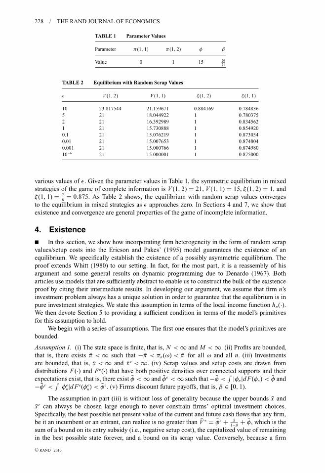
where F−1(ξ (ω)) = 2ξ (ω) − 1. There are nine cases to be considered, depending on whetherξ (1, 1) is equal to 0, between 0 and 1, or equal to 1 and on whether ξ (1, 2) is equal to 0, between0 and 1, or equal to 1. Table 1 specifies parameter values.

A case-by-case analysis shows that, with random scrap values, there always exists a uniquesymmetric equilibrium. If ε > 5, the equilibrium involves 0 < ξ (1, 2) < 1 and 0 < ξ (1, 1) < 1,and if ε ≤ 5, it involves ξ (1, 2) = 1 and 0 < ξ (1, 1) < 1. Table 2 describes the equilibrium for

17 To see this, note that the first and second derivatives of the right-hand side of the Bellman equation are given byd(.)

d ξ (ω)= −φ − εF−1(ξ (ω)) + φ(ω) and d2(.)

d ξ (ω)2 = −ε 1F ′ (F−1(ξ (ω)))

, respectively.18 Besides the uniform distribution, many others yield a closed-form expression, including triangular and Beta

distributions.

C© RAND 2010.


TABLE 1 Parameter Values

Parameter π (1, 1) π (1, 2) φ β

Value 0 1 15 2021

TABLE 2 Equilibrium with Random Scrap Values

ε V (1, 2) V (1, 1) ξ (1, 2) ξ (1, 1)

10 23.817544 21.159671 0.884169 0.7848365 21 18.044922 1 0.7803752 21 16.392989 1 0.8345621 21 15.730888 1 0.8549200.1 21 15.076219 1 0.8730340.01 21 15.007653 1 0.8748040.001 21 15.000766 1 0.87498010−6 21 15.000001 1 0.875000

various values of ε. Given the parameter values in Table 1, the symmetric equilibrium in mixedstrategies of the game of complete information is V (1, 2) = 21, V (1, 1) = 15, ξ (1, 2) = 1, andξ (1, 1) = 7

8= 0.875. As Table 2 shows, the equilibrium with random scrap values converges

to the equilibrium in mixed strategies as ε approaches zero. In Sections 4 and 7, we show thatexistence and convergence are general properties of the game of incomplete information.

4. Existence

� In this section, we show how incorporating firm heterogeneity in the form of random scrapvalues/setup costs into the Ericson and Pakes’ (1995) model guarantees the existence of anequilibrium. We specifically establish the existence of a possibly asymmetric equilibrium. Theproof extends Whitt (1980) to our setting. In fact, for the most part, it is a reassembly of hisargument and some general results on dynamic programming due to Denardo (1967). Botharticles use models that are sufficiently abstract to enable us to construct the bulk of the existenceproof by citing their intermediate results. In developing our argument, we assume that firm n’sinvestment problem always has a unique solution in order to guarantee that the equilibrium is inpure investment strategies. We state this assumption in terms of the local income function hn(·).We then devote Section 5 to providing a sufficient condition in terms of the model’s primitivesfor this assumption to hold.

We begin with a series of assumptions. The first one ensures that the model’s primitives arebounded.

Assumption 1. (i) The state space is finite, that is, N < ∞ and M < ∞. (ii) Profits are bounded,that is, there exists π < ∞ such that −π < πn(ω) < π for all ω and all n. (iii) Investmentsare bounded, that is, x < ∞ and x e < ∞. (iv) Scrap values and setup costs are drawn fromdistributions F(·) and Fe(·) that have both positive densities over connected supports and theirexpectations exist, that is, there exist φ < ∞ and φe < ∞ such that −φ <

∫ |φn|d F(φn) < φ and−φe <

∫ |φen|d Fe(φe

n) < φe. (v) Firms discount future payoffs, that is, β ∈ [0, 1).

The assumption in part (iii) is without loss of generality because the upper bounds x andx e can always be chosen large enough to never constrain firms’ optimal investment choices.Specifically, the best possible net present value of the current and future cash flows that any firm,be it an incumbent or an entrant, can realize is no greater than V ∗ = φe + π

1−β+ φ, which is the

sum of a bound on its entry subsidy (i.e., negative setup cost), the capitalized value of remainingin the best possible state forever, and a bound on its scrap value. Conversely, because a firm

C© RAND 2010.


always has the option of investing zero, it can guarantee that the net present value of its currentand future cash flows is no worse than −V ∗. Because no firm is ever willing to invest more thanβ(V ∗ − (−V ∗)) = 2β V ∗ in order to reap the best instead of the worst possible net present value,upper bounds on investment in excess of 2β V ∗ never constrain firms’ optimal choices.

The assumption in part (iv) admits distributions F(·) and Fe(·) with either bounded orunbounded support. From a theorist’s perspective, it is natural to assume bounded supportsbecause unbounded supports essentially stipulate that some agent is willing to pay an arbitrarilylarge amount to acquire the assets of a firm that makes bounded profits from product marketcompetition. From an empiricist’s perspective, unbounded supports (as assumed by Aguirregabiriaand Mira, 2007 and Pesendorfer and Schmidt-Dengler, 2008) may be attractive because theyguarantee that in the data there cannot be an observation that has zero probability of occurring.

Next we assume continuity of the transition function P(·). Similar continuity assumptionsare commonplace in the literature on dynamic stochastic games (see Mertens, 2002).

Assumption 2. P(ω′, ω, χ (ω, φ), x(ω)) is a continuous function of x(ω) for all ω′, ω, and allχ (ω, φ).

Observe from equation (10) that current profit is additively separable from investment.The continuity of the transition function P(·) in x(ω) therefore ensures the continuity of thelocal income function hn(·) in x(ω). In addition, hn(·) is continuous in ξ (ω) because, analogousto equation (1), firm n integrates out over all possible realizations of its rivals’ exit and entrydecisions χ−n(ω, φ−n) to obtain the probability that the industry transits from state ω to state ω′.Observe further that hn(·) is always continuous in Vn because Vn enters hn(·) in equation (10) viathe expected value of firm n’s future cash flows, E {Vn(ω′)|·}. We record these observations forlater use.

Proposition 1. Under Assumption 2, hn(ω, u(ω), Vn) is a continuous function of u(ω) and Vn forall ω and all n.

Due to the random scrap values/setup costs, our model is formally a dynamic stochasticgame with a finite state space and a continuum of actions given by the probability that anincumbent firm remains in the industry/a potential entrant enters the industry and the set of feasibleinvestment choices. Under Assumptions 1 and 2, standard arguments (e.g., Federgruen, 1978;Whitt, 1980) yield the existence of an equilibrium in mixed strategies. However, mixed strategiesover continuous actions are infeasible to compute. To guarantee the existence of an equilibrium inpure investment strategies, we make the additional assumption that firm n’s investment problemalways has a unique solution.

Assumption 3. A unique xn(ω) exists that attains the maximum of hn(ω, 1, xn(ω), u−n(ω), Vn) forall u−n(ω), Vn, ω, and all n.19

In Section 5, we provide a sufficient condition for Assumption 3 to hold in terms of themodel’s primitives. Specifically, we define UIC admissibility of the transition function P(·) andprove that this condition ensures uniqueness of investment choice. Therefore, Assumption 3holds and an equilibrium that is amenable to computation exists. Constructing our argumentin this modular form makes it simple and transparent for other researchers to insert alternativesufficient conditions for uniqueness of investment choice into our proof and immediately obtainexistence.

Recall that we assume entry and exit decisions are implemented before investmentdecisions are carried out. Thus, firm n chooses xn(ω) to maximize hn(ω, 1, xn(ω), u−n(ω), Vn)in accordance with equations (3) and (6), and the resulting investment choice also maximizes

19 Assumption 3 can be weakened to hold for all possible maximal return functions V ∗n,u−n

∈ [−V ∗, V ∗]|S|.

C© RAND 2010.


hn(ω, ξn(ω), xn(ω), u−n(ω), Vn) for all ξn(ω) > 0, u−n(ω), Vn, ω, and all n. Clearly any investmentwould be optimal whenever an incumbent firm exits for sure or a potential entrant stays out forsure. Consequently, we adopt the following convention: if ξn(ω) = 0, then we take xn(ω) to havethe value alluded to in Assumption 3. It follows that hn(ω, ξn(ω), xn(ω), u−n(ω), Vn) attains itsmaximum for a unique value of xn(ω) independent of the value of ξn(ω). This is a natural conven-tion because if there were even the slightest chance that firm n would remain in the industry eventhough it sets ξn(ω) = 0, then the firm would want to choose this value of xn(ω) as its investment.

The above assumptions ensure existence of an equilibrium.

Proposition 2. Under Assumptions 1, 2, and 3, an equilibrium exists in cutoff entry/exit and pureinvestment strategies.

The proof is based on the following idea.20 Fix strategies u−n and consider firm n’s problem.Because its competitors’ strategies are fixed, firm n has to solve a decision problem (as opposedto a game problem). We can thus employ dynamic programming techniques to analyze the firm’sproblem. In particular, a contraction mapping argument establishes that the firm’s best reply toits competitors’ strategies is well defined. It remains to show that there exists a fixed point in thefirms’ best-reply correspondences.

Before stating the proof of Proposition 2, we introduce and discuss a number of constructs.We start with the decision problem. Let Vn denote the space of bounded |S| × 1 vectors endowedwith the sup norm. Fix u−n ∈ U−n and define the maximal return operator H ∗

n,u−n: Vn → Vn

pointwise by

(H ∗n,u−n

Vn)(ω) = supun (ω)∈Un (ω)

hn(ω, un(ω), u−n(ω), Vn).

The number (H ∗u−n

Vn)(ω) represents the return to firm n in state ω when firm n chooses its optimalaction while the other firms use actions u−n(ω) and firm n’s future returns are described by Vn .Note that the right-hand side of the above equation coincides with the right-hand side of theBellman equation (9).

Because profits and investments are bounded and the expectations of scrap values and setupcosts exist by Assumption 1, H ∗

n,u−ntakes bounded vectors into bounded vectors. Application

of Blackwell’s sufficient conditions (Blackwell, 1965, Theorem 5; see also Stokey and Lucas,1989, Theorem 3.3) shows that H ∗

n,u−nis a contraction with modulus β. First, inspection of

equation (10) shows that Vn(ω) ≥ Vn(ω) for all ω implies (H ∗n,u−n Vn)(ω) ≥ (H ∗

n,u−nVn)(ω) for all

ω (“monotonicity”). Second, given a constant c ≥ 0, (H ∗n,u−n(Vn + c))(ω) ≤ (H ∗

n,u−n Vn)(ω) + βcfor all ω (“discounting”).

Because H ∗n,u−n

is a contraction, the contraction mapping theorem (see Stokey and Lucas,1989, Theorem 3.2) implies that there exists a unique V ∗

n,u−n∈ Vn that satisfies V ∗

n,u−n= H ∗

n,u−nV ∗

n,u−n

or, equivalently,

V ∗n,u−n

(ω) = supun (ω)∈Un (ω)

hn(ω, un(ω), u−n(ω), V ∗n,u−n

) (14)

for all ω. The fixed point V ∗n,u−n

of H ∗n,u−n

is called the maximal return function given policies u−n;it should be thought of as a mapping from U−n into Vn . Clearly, given u−n , the maximal returnfunction V ∗

n,u−nsolves the Bellman equation (9); it plays a major role in our existence proof.

Before proceeding to the existence proof, we introduce and discuss another operator. Fixu ∈ U and define the return operator Hn,u : Vn → Vn pointwise by

(Hn,u Vn)(ω) = hn(ω, u(ω), Vn).

The number (Hu Vn)(ω) represents the return to firm n in state ω when the firms use actionsu(ω) and Vn describes firm n’s future returns. Like H ∗

n,u−n, Hn,u is a contraction with modulus β

20 Given that standard arguments establish the existence of an equilibrium in mixed strategies, it actually sufficesto show that a firm is never willing to mix. The reason that we start from first principles is that we need the machineryfrom the proof of Proposition 2 for the proofs of Propositions 3, 5, and 6.

C© RAND 2010.


that takes bounded vectors into bounded vectors. Hence, a unique Vn,u ∈ Vn exists that satisfiesVn,u = Hn,u Vn,u , that is,

Vn,u(ω) = hn(ω, u(ω), Vn,u) (15)

for all ω. The fixed point Vn,u of Hn,u is called the return function given policies u; it should bethought of as a mapping from U into Vn .

The return function Vn,u and the maximal return function V ∗n,u−n

are tightly connected.Because the return operator Hn,u is monotonic (meaning that Vn(ω) ≥ Vn(ω) for all ω implies(Hn,u Vn)(ω) ≥ (Hn,u Vn)(ω) for all ω), Denardo (1967) establishes that

V ∗n,u−n

(ω) = supun∈Un

Vn,un ,u−n (ω) (16)

for all ω, where Vn,un ,u−n is the fixed point of the return operator given policy (un, u−n).With this machinery in place, we turn to the game problem. Consider the mapping

ϒn : U−n → Un defined by

ϒn(u−n) ={

un ∈ Un : un(ω) ∈ arg supun (ω)∈Un (ω)

hn(ω, un(ω), u−n(ω), V ∗n,u−n

) for all ω

}. (17)

ϒn(·) is the best-reply correspondence of firm n and ϒn(u−n) is the set of best replies of firm ngiven rivals’ policies u−n . Consider further the mapping ϒ : U → U obtained by stacking thesebest-reply correspondences. ϒ(u) = (ϒ1(u−1), . . . , ϒN (u−N )) is the set of best replies of firm 1given rivals’ policies u−1, those of firm 2 given rivals’ policies u−2, etc. An equilibrium exists ifthere is a u ∈ U such that u ∈ ϒ(u). To show that such a u exists, we show that ϒ(·) is, in fact, acontinuous function to which Brouwer’s fixed-point theorem applies.

Proof of Proposition 2. We begin by establishing that ϒ(·) is nonempty and upper hemicon-tinuous. Given policies u−n , firm n’s maximal return function V ∗

n,u−nis well defined due to

Assumption 1, as shown above. Fix ω. Proposition 1 states that firm n’s local income functionhn(ω, u(ω), Vn) is continuous in u(ω) and Vn. The maximand, hn(ω, un(ω), u−n(ω), V ∗

n,u−n), in the

definition of ϒn(·) in equation (17) is therefore continuous in un(ω) and u−n if firm n’s maximalreturn function V ∗

n,u−nis continuous in u−n . That this is so is established through appeal to two

lemmas by Whitt (1980).In Lemma 3.2 he states that if Hn,u Vn is continuous in u for all Vn , then the return function

Vn,u is continuous in u.21 This establishes that Vn,u is a continuous function of u. In Lemma 3.1he states that if Un(ω), firm n’s set of feasible actions in state ω, is a compact metric space forall ω, if the state space S is countable, and if the return function Vn,u is continuous in u, thensupun∈Un

Vn,un ,u−n (ω) is continuous in u−n for all ω. These requirements are satisfied. Equation (16)thus implies that V ∗

n,u−n(ω) is continuous in u−n for all ω. This, of course, implies that firm n’s

maximal return function V ∗n,u−n

is continuous in u−n .Because hn(ω, un(ω), u−n(ω), V ∗

n,u−n) is continuous in un(ω) and u−n and Un(ω) is compact

and independent of u−n , the theorem of the maximum (see Stokey and Lucas, 1989, Theorem 3.6)implies that arg supun (ω)∈Un (ω) hn(ω, un(ω), u−n(ω), V ∗

n,u−n) is nonempty and upper hemicontinuous

in u−n . Because ω was arbitrary, this establishes that ϒn(·) is a nonempty and upper hemicontinuouscorrespondence that maps U−n into Un . Hence, ϒ(·) is a nonempty and upper hemicontinuouscorrespondence that maps U into U .

We next show that ϒ(·) is single valued. Recall that, given policies u−n , firm n’s maximalreturn function V ∗

n,u−nis well defined, and consider firm n’s best reply in state ω. Uniqueness

of the investment choice follows from Assumption 3 and our convention covering the specialcase of ξn(ω) = 0. This, in turn, implies that equations (3) and (6) give unique exit and entry

21 It is immediate to verify that the return operator Hn,u satisfies the boundedness, monotonicity, and contractionassumptions in Whitt (1980). Whitt (1980) denotes the return function Vn,u by vδ(·, i) and the maximal return functionV ∗

n,u−nby fδ(·, i). We set Wn = Vn to obtain a special case of Lemma 3.2 in Whitt (1980).

C© RAND 2010.


cutoffs, φn(ω) and φen(ω). Given that these cutoffs are unique, the corresponding exit and entry

probabilities, ξn(ω) = F(φn(ω)) (if ωn �= M + 1) and ξn(ω) = Fe(φen(ω)) (if ωn = M + 1), must

be unique. Because ω was arbitrary, this establishes that ϒn(·) and hence ϒ(·) is single valued.Because ϒ(·) is nonempty, single valued, and upper hemicontinuous, it is, in fact, a

continuous function that maps the nonempty, convex, and compact set U into itself. Brouwer’sfixed-point theorem therefore applies: a u ∈ U exists such that u ∈ ϒ(u). Q.E.D.

5. A sufficient condition for pure investment strategies

� Assumption 3 requires that the local income function hn(ω, 1, xn(ω), u−n(ω), Vn) is maxi-mized at a unique investment choice xn(ω) for all u−n(ω), Vn, ω, and all n. Fortunately, a judiciouschoice of transition probabilities guarantees that the investment choice is indeed unique. In thissection, we first define UIC admissibility of the transition function P(·) and show in Proposition 3that if this condition on the model’s primitives is satisfied, then Assumption 3 holds. We thenprovide a series of examples of transition functions that are UIC admissible and provide areasonable amount of flexibility.

Condition 1. The transition function P(·) is unique investment choice (UIC) admissible if, forall χ−n(ω, φ−n), x(ω), ω′, ω, and all n, the probability P(ω′, ω, 1, χ−n(ω, φ−n), x(ω)) that theindustry moves from state ω to state ω′ given that firm n remains in the industry (or enters theindustry if firm n is an entrant rather than an incumbent) can be written in a separable form as

Kn (ω′, ω, χ−n (ω, φ−n) , x−n(ω)) Qn(ω, xn(ω)) + Ln (ω′, ω, χ−n (ω, φ−n) , x−n(ω)) , (18)

where Qn(ω, x(ω)) is twice differentiable, strictly increasing, and strictly concave in xn(ω), thatis,

d

dxn(ω)Qn(ω, xn(ω)) > 0,

d2

dxn(ω)2Qn(ω, xn(ω)) < 0 (19)

for all xn(ω) ∈ [0, x] (or xn(ω) ∈ [0, x e] if firm n is an entrant rather than an incumbent).22

UIC admissibility ensures that firm n’s local income function hn(. . . , 1, xn(ω), . . .) either isstrictly concave—and therefore has a unique maximizer—in the interval [0, x] (or in the interval[0, x e] if firm n is an entrant rather than an incumbent) or that the unique maximizer is a cornersolution. This establishes the following.

Proposition 3. If the transition function P(·) is UIC admissible (Condition 1), then Assumption 3holds.

Proof. Because the proof for a potential entrant is the same with x e replacing x , we focus onthe investment problem of an incumbent firm in what follows. UIC admissibility ensures that theexpected value of firm n’s future cash flow, E {Vn(ω′)|ω,ω′

n �= M + 1, ξ−n(ω), x(ω)}, in its localincome function hn(. . . , 1, xn(ω), . . .) can be written in a separable form as

An(ω, u−n(ω), Vn)Qn(ω, xn(ω)) + Bn(ω, u−n(ω), Vn). (20)

To see this, recall from equation (1) that firm n has to integrate out over all possible realizationsof its rivals’ exit and entry decisions to obtain the probability that the industry moves from stateω to state ω′. Hence,

22 Condition 1 can be generalized to allow for Q(·) to depend on x−n(ω).

C© RAND 2010.


∑ω′∈S

Vn(ω′)∑

ι−n∈{0,1}N−1

P(ω′, ω, 1, ι−n, x(ω))∏k �=n

ξk(ω)ιk (1 − ξk(ω))1−ιk

=∑ω′∈S

Vn(ω′)∑

ι−n∈{0,1}N−1

[Kn (ω′, ω, ι−n, x−n(ω)) Qn(ω, xn(ω)) + Ln (ω′, ω, ι−n, x−n(ω))]

×∏k �=n


=[∑

ω′∈S

Vn(ω′)∑

ι−n∈{0,1}N−1

Kn (ω′, ω, ι−n, x−n(ω))∏k �=n


]︸︷︷︸

An (ω,u−n (ω),Vn )

Qn(ω, xn(ω))

+[∑

ω′∈S

Vn(ω′)∑

ι−n∈{0,1}N−1

Ln (ω′, ω, ι−n, x−n(ω))∏k �=n


]︸︷︷︸

Bn (ω,u−n (ω),Vn )

,

where the first equality uses the separability condition (18).Next we differentiate hn(. . . , 1, xn(ω), . . .) with respect to xn(ω). By virtue of equation (20),

the first-order condition for an unconstrained solution to firm n’s investment problem is

−1 + β An(ω, u−n(ω), Vn)d

dxn(ω)Qn(ω, xn(ω)) = 0.

There are two cases to consider. First suppose that An(ω, u−n(ω), Vn) > 0. If there existsa solution to the first-order condition in [0, x], say xn(ω), then it must be unique because theobjective function is strictly concave on [0, x] in light of the derivative condition (19). Hence,xn(ω) = xn(ω) is the unique maximizer. If there does not exist a solution to the first-order conditionin [0, x], then the objective function is either strictly decreasing or strictly increasing on [0, x].In the former case the unique maximizer is xn(ω) = 0, and in the latter case it is xn(ω) = x .

Next suppose that An(ω, u−n(ω), Vn) ≤ 0. The objective function is strictly decreasing.Hence, the unique maximizer is xn(ω) = 0. Q.E.D.

UIC admissibility allows for much more flexibility in the transition probabilities than thesimple schemes seen in the extant literature where each firm each period is restricted to move upone state, stay the same, or drop down one state. We demonstrate this with a series of increasinglycomplex examples all involving an industry with N = 2 firms, M ≥ 3 “active” states, and noentry and exit.

� Example: independent transitions to immediately adjacent states. Consider a game ofcapacity accumulation similar to that in Besanko and Doraszelski (2004). A firm’s state describesits capacity. In each period, the firm decides how much to spend on an investment project in orderto add to its capacity. If firm n invests xn(ω) ≥ 0, then the probability that its investment projectsucceeds is

pn = αxn(ω)

1 + αxn(ω),

where the parameter α > 0 measures the effectiveness of investment. Depreciation tends to offsetinvestment, and we assume that each firm is independently hit by a depreciation shock withprobability δ. The transition probabilities at an interior state ω ∈ {2, . . . , M − 1}2 are given inTable 3.

Without loss of generality, consider firm 1. The probability of remaining in state ω can bewritten as

C© RAND 2010.


TABLE 3 Transition Probabilities for Independent Transitions to Immediately Adjacent States

ω′2 = ω2 + 1 ω′

2 = ω2 ω′2 = ω2 − 1

ω′1 = ω1 + 1 (1 − δ)p1(1 − δ)p2 (1 − δ)p1[δ p2 + (1 − δ)(1 − p2)] (1 − δ)p1δ p2

ω′1 = ω1 [δ p1 + (1 − δ)(1 − p1)]

× (1 − δ)p2

[δ p1 + (1 − δ)(1 − p1)]

× [δ p2 + (1 − δ)(1 − p2)]

[δ p1 + (1 − δ)(1 − p1)]

× δ p2

ω′1 = ω1 − 1 δ(1 − p1)(1 − δ)p2 δ(1 − p1)[δ p2 + (1 − δ)(1 − p2)] δ(1 − p1)δ p2

TABLE 4 Transition Probabilities for Dependent Transitions to Immediately Adjacent States

ω′2 = ω2 + 1 ω′

2 = ω2 ω′2 = ω2 − 1

ω′1 = ω1 + 1 (1 − δ)p1 p2 (1 − δ)p1(1 − p2) 0

ω′1 = ω1 (1 − δ)(1 − p1)p2 (1 − δ)(1 − p1)(1 − p2) + δ p1 p2 δ p1(1 − p2)

ω′1 = ω1 − 1 0 δ(1 − p1)p2 δ(1 − p1)(1 − p2)

[δ p1 + (1 − δ)(1 − p1)][δ p2 + (1 − δ)(1 − p2)]

= [2δ − 1][δ p2 + (1 − δ)(1 − p2)]︸︷︷︸K1(ω,ω,x2(ω))

p1︸︷︷︸Q1(ω,x1(ω))

+ [1 − δ][δ p2 + (1 − δ)(1 − p2)]︸︷︷︸L1(ω,ω,x2(ω))

.

This expression satisfies the separability condition (18), as do the corresponding expressions forthe probabilities of moving to some other state ω′ �= ω. In addition, the derivative condition (19)is satisfied because

d

dx1(ω)Q1(ω, x1(ω)) = α

(1 + αx1(ω))2> 0,

d2

dx1(ω)2Q1(ω, x1(ω)) = − 2α2

(1 + αx1(ω))3< 0.

� Example: dependent transitions to immediately adjacent states. Next we introducecorrelation into firms’ transitions by replacing the firm-specific depreciation shocks of the aboveexample by an industry-wide depreciation shock (e.g., Pakes and McGuire, 1994). Decompose, forpurposes of exposition, the transition of each firm into two stages. In the first stage, the probabilitythat firm n’s state increases by one is again given by pn . In the second stage, a depreciation shockreduces the states of all firms by one with probability δ. The transition probabilities at an interiorstate ω ∈ {2, . . . , M − 1}2 are given in Table 4.

For the sake of brevity, we just spell out the probability of remaining in state ω,

(1 − δ)(1 − p1)(1 − p2) + δ p1 p2 = [δ − 1 + p2]︸︷︷︸K1(ω,ω,x2(ω))

p1︸︷︷︸Q1(ω,x1(ω))

+ [(1 − δ)(1 − p2)]︸︷︷︸L1(ω,ω,x2(ω))

,

and note that conditions (18) and (19) are again both satisfied.

� Example: dependent transitions to arbitrary states. Using the above two-stage decom-position, much more flexible transitions can be constructed. In the first stage, firm n’s investmentxn(ω) determines a set of transition probabilities to all possible “active” states. For example, theprobability that firm n moves from its initial state ωn to the intermediate state ωn ∈ {1, . . . , M}may be

C© RAND 2010.


⎧⎪⎪⎪⎪⎪⎪⎪⎪⎪⎪⎪⎪⎪⎪⎨⎪⎪⎪⎪⎪⎪⎪⎪⎪⎪⎪⎪⎪⎪⎩

ζn,ωn ,1 + ηn,ωn ,1 pn if ωn = 1,

......

...

ζn,ωn ,ωn−1 + ηn,ωn ,ωn−1 pn if ωn = ωn − 1,

ζn,ωn ,ωn + ηn,ωn ,ωn pn if ωn = ωn,

ζn,ωn ,ωn+1 + ηn,ωn ,ωn+1 pn if ωn = ωn + 1,

......

...

ζn,ωn ,M + ηn,ωn ,M pn if ωn = M,

where xn(ω) affects the probability of a transition from state ωn to state ωn either positively ofnegatively depending on the sign of ηn,ωn ,ωn .23 In the second stage, the industry transits fromits intermediate state ω to its final state ω′ according to some arbitrary, exogenously givenprobabilities that may depend on ω.

Clearly, pn does not have to equal αxn (ω)1+αxn (ω)

; it can be of any form that satisfies the derivativecondition (19). For example, let

pn = 1 − e−αxn (ω),

where α > 0. As another example, let

pn =arctan

(2α1xn(ω) + α2√

4 − α22

)− arctan

(α2√

4 − α22

)

π

2− arctan

(α2√

4 − α22

) ,

where α1 > 0 and 0 ≤ α2 < 2. Then pn is increasing in α1 (just as αxn (ω)1+αxn (ω)

and 1 − eαxn (ω) areincreasing in α) and increasing (decreasing) in α2 to the left (right) of xn(ω) = 1

α1. That is,

whereas increasing α1 makes investments of all sizes more effective, increasing α2 makes smallinvestments more and large ones less effective. In addition, xn(ω) = 1

α1implies pn = 1

2. Hence,

increasing α2 preserves the median but increases the spread of pn as measured, for example, bythe interquartile range.

UIC admissibility is a sufficient condition and, if it fails, uniqueness of investment choicecan often be achieved by other means. Purification is again a very valuable tool. In particular, apart of the subsequent literature has assumed that the cost of investment is randomly drawn andprivately known. Ryan (2006) and Besanko, Doraszelski, Lu, and Satterthwaite (2010) extend ourhandling of entry and exit to the case of discrete (or “lumpy”) investment. Their models remainscomputationally tractable because the equilibrium is in cutoff investment strategies. Focusingon the case of continuous investment, Jenkins, Liu, Matzkin, and McFadden (2004) restrict thefunctional form of per-period payoffs to ensure that a firm’s optimal investment level is almostalways unique given a realization of the cost of investment. Again its rivals perceive the firm asthough it were following a mixed strategy, thereby facilitating the existence of an equilibrium,although computing these perceptions—as one must in order to determine the rivals’ best repliesto them—becomes somewhat more involved.

6. Symmetry

� In Section 4, we established the existence of a possibly asymmetric equilibrium. We nowshow that if the model’s primitives satisfy an additional symmetry assumption, then a symmetricequilibrium exists.

23 The parameters ζn,ωn ,ωn and ηn,ωn ,ωn must be chosen to ensure that the probabilities stay in the unit interval for allxn(ω) ∈ [0, x] and sum to one. In particular, this requires

∑Mωn =1 ζn,ωn ,ωn = 1 and

∑Mωn =1 ηn,ωn ,ωn = 0.

C© RAND 2010.


Informally, the notion of symmetry in Ericson and Pakes (1995) is this: consider an industrywith five firms and suppose that when firm 2 is in state 3 and the other four firms are in states 1,3, 3, and 6, it invests 50. Symmetry means that when firm 4 is in state 3 and the other four firmsare in states 1, 3, 3, and 6, it also invests 50. Thus, in a symmetric equilibrium, a firm’s policy isa common function of its own state and the distribution of its rivals’ states.

To formalize this notion of symmetry, let κ = (κ1, . . . , κN ) be a permutation of (1, . . . , N ).The policy functions u = (u1, . . . , uN ) are symmetric if

un(ωκ1 , . . . , ωκn−1 , ωκn , ωκn+1 , . . . , ωκN ) = uκn (ω1, . . . , ωn−1, ωn, ωn+1, . . . , ωN ) (21)

for all ω, n, and all κ . We say that an equilibrium is symmetric if its policy functions are symmetric.Moreover, in a symmetric equilibrium, the value functions V = (V1, . . . , VN ) are symmetric andsatisfy the analog of equation (21).

This definition implies two key properties that capture the essence of symmetry:

(i) If the states of two firms are the same, then their actions must be the same. Forexample, if ω = (2, 3, 3), then set κ = (2, 3, 1) in equation (21) to obtain u2(3, 3, 2) =u2(ω2, ω3, ω1) = u3(ω1, ω2, ω3) = u3(2, 3, 3).

(ii) A firm does not care about the identity of its rivals; hence, the firm’s action must be thesame after its rivals’ exchange states. For example, if ω = (2, 3, 4), then set κ = (3, 2, 1)in equation (21) to obtain u2(4, 3, 2) = u2(ω3, ω2, ω1) = u3(ω1, ω2, ω3) = u2(2, 3, 4).

Inspection shows that these properties imply the notion of symmetry in Ericson and Pakes(1995): a firm’s policy is a common function of its own state and the distribution of its rivals’states.

One of the reasons symmetry is important is that it eases the computational burdenconsiderably. Instead of having to compute value and policy functions for all firms, undersymmetry it suffices to compute value and policy functions for one firm, say firm 1. To seethis, let κ = (n, 2, . . . , n − 1, 1, n + 1, . . . , N ) in equation (21) to obtain

un(ωn, ω2, . . . , ωn−1, ω1, ωn+1, . . . , ωN ) = u1(ω1, ω2, . . . , ωn−1, ωn, ωn+1, . . . , ωN ), (22)

and similarly for the value function. That is, the value and policy of firm n is the same as thevalue and policy of firm 1 had their states been interchanged. In addition, symmetry reduces thesize of the state space on which the value and policy functions of firm 1 are defined because firm1 does not care about the identity of its competitors. To see this, let n = 1 and κ = (1, 2, . . . , k −1, l, k + 1, . . . , l − 1, k, l + 1, . . . , N ) with k ≥ 2 and l ≥ 2 in equation (21) to obtain

u1(ω1, ω2, . . . , ωl, . . . , ωk, . . . , ωN ) = u1(ω1, ω2, . . . , ωk, . . . , ωl, . . . , ωN ), (23)

and similarly for the value function. That is, only the firm’s own state and the distribution of rivals’states matter. This latter property is commonly referred to as anonymity or exchangeability.24

We are now ready to state our symmetry assumption.

Assumption 4. The local income functions are symmetric, that is,

hn(ωκ1, . . . , ωκN , uκ1 (ω), . . . , uκN (ω), Vn) = hκn (ω1, . . . , ωN , u1(ω), . . . , uN (ω), Vκn ) (24)

for all u(ω), symmetric V , ω, n, and all κ .

Note that the value functions that enter the local income functions are themselves symmetric.Some further explanation may be helpful. A permutation κ shuffles firms’ states, actions,

and value functions in a way that preserves the values of their local income functions according

24 Equations (22) and (23) are often together taken as the definition of symmetry (e.g., Doraszelski and Pakes,2007). It is easy to see that they are equivalent to our notion of symmetry in equation (21). Working with equation (21)instead of equations (22) and (23) simplifies the notation in the remainder of this section.

C© RAND 2010.


to the principle that identical actions in identical situations yield identical payoffs. Let n = 2 andκ = (2, 3, 1) in equation (24) to obtain

h2(ω2, ω3, ω1, u2(ω), u3(ω), u1(ω), V2) = h3(ω1, ω2, ω3, u1(ω), u2(ω), u3(ω), V3).

On the left-hand side, firm 2 is in state ω3 and takes action u3(ω) while it faces two rivals, one instate ω1 and one in state ω2. On the right-hand side, firm 3 is in state ω3 and takes action u3(ω)while it faces two rivals, one in state ω1 and one in state ω2. Because the state of firm 2 on theleft-hand side is that of firm 3 on the right-hand side and the distribution over states and actions offirm 2’s rivals on the left-hand side is that of firm 3’s rivals on the right-hand side, their respectivesituations are identical.

Although we have stated Assumption 4 in terms of the local income functions to facilitatethe adaptation of our existence proof to other models, it is readily tied to the model’s primitives.

Condition 2. The model’s primitives are symmetric if (i) the profit functions are symmetric, thatis,

πn(ωκ1 , . . . , ωκN ) = πκn (ω1, . . . , ωN )

for all ω, n, and all κ and (ii) the transition function is symmetric, that is,

P(ω′κ1, . . . , ω′

κN, ωκ1 , . . . , ωκN , χκ1 (ω, φκ1 ), . . . , χκN (ω, φκN ), xκ1 (ω), . . . , xκN (ω))

= P(ω′1, . . . , ω

′N , ω1, . . . , ωN , χ1(ω, φ1), . . . , χN (ω, φN ), x1(ω), . . . , xN (ω))

for all χ (ω, φ), x(ω), ω′, ω, and all κ .

Proposition 4. If the model’s primitives are symmetric (Condition 2), then Assumption 4 holds.

The proof of Proposition 4 is straightforward but tedious and therefore omitted. Notethat in the special case of independent transitions, part (ii) of Condition 2 is satisfiedwhenever the factors Pn(·) of the transition function P(·) are the same across firms, that is,Pn(ω′

n, ωn, χn(ω, φn), xn(ω)) = P1(ω′n, ωn, χn(ω, φn), xn(ω)) for all n.

Together with Assumptions 1, 2, and 3 in Section 4, Assumption 4 ensures existence of asymmetric equilibrium.

Proposition 5. Under Assumptions 1, 2, 3, and 4, a symmetric equilibrium exists in cutoffentry/exit and pure investment strategies.

The idea of the proof is as follows. Symmetry allows us to restrict attention to the best-replycorrespondence of firm 1. To enforce the anonymity that symmetry implies, we redefine the statespace employing Ericson and Pakes’ (1995) notion that symmetry means each firm’s investmentis a common function of its own state and the distribution of its rivals’ states. This reduced statespace makes it impossible for firm 1 to tailor its policy to the identity of its competitors. Anargument analogous to the proof of Proposition 2 shows that there exists a fixed point to thebest-reply correspondence of firm 1. We use this fixed point to construct a candidate equilibriumby specifying symmetric policies for all firms. The associated value functions are also symmetric.Finally, to complete the argument, we exploit the symmetry of the local income functions to showthat no firm has an incentive to deviate from the candidate equilibrium.

In preparation for proving Proposition 5, we introduce the necessary notation to construct thecandidate equilibrium. To understand our notation, it is helpful to keep in mind that the candidateequilibrium will be symmetric. We begin with defining the reduced state space. Consider firm n andstate ω. Define σn = (σn,1, . . . , σn,M , σn,M+1), where σn,m denotes the number of competitors of firm

n that are in state m (excluding firm n), and � ={σn ∈ {0, 1, . . . , N − 1}|∑M+1

m=1 σn,m = N − 1}

to be the set of values that σn can take on. Rewrite ω as (ωn, σn). Let S◦ = � × � denote thereduced state space and S = �N the full state space. Define a function τn : S → S◦ such thatτn(ω) = (ωn, σn); it maps the full to the reduced state space. For example, if N = 4, M = 3,and ω = (3, 2, 2, 4), then (ω1, σ1) = τ1(ω) = (3, 0, 2, 0, 1) and (ω3, σ3) = τ3(ω) = (2, 0, 1, 1, 1).

C© RAND 2010.


Note that no information is lost in going from the full to the reduced state space, provided that theequilibrium is symmetric. In particular, τ1(ω) contains all the information in ω that is required toevaluate the value and policy functions of firm 1. Note also that in general the reduced state spaceis considerably smaller than the full state space: it has just |S◦| = (M + 1)(M+N−1

N−1) < (M + 1)N =

|S| states.25

Define the inverse function τ−1n : S◦ → S such that ω = τ−1

n (ωn, σn) is a fixed selectionfrom the set {ω|(ωn, σn) = τn(ω)}. We adopt the convention that ω = τ−1

n (ωn, σn) satisfies ω1 ≤ω2 ≤ · · · ≤ ωn−1 ≤ ωn+1 ≤ · · · ≤ ωN . Observe that, if ω = τ−1

n (τn(ω)), then ω is obtained from ω

by rearranging the elements of ω−n . For example, (3, 2, 2, 5) = τ−11 (τ1(3, 2, 5, 2)), (2, 2, 3, 5) =

τ−12 (τ2(3, 2, 5, 2)), and so forth. A state ω is called canonical if and only if ω = τ−1

1 (ω1, σ1) forsome (ω1, σ1). We use the symbol ˇ to distinguish canonical states in the remainder of this section.

Next we redefine actions, strategies, and payoffs on the reduced state space. We use thesymbol ◦ to distinguish objects defined on the reduced state space from the correspondingobjects defined on the full state space. For example, we write u◦

1(ω1, σ1) ∈ U ◦1 (ω1, σ1) instead

of u1(ω) ∈ U1(ω), where U ◦1 (ω1, σ1) = U1(τ

−11 (ω1, σ1)) because U1(ω) merely hinges on ω1 (see

equation (8)). By construction, a strategy u◦1 = ×(ω1,σ1)∈S◦u◦

1(ω1, σ1) ∈ ×(ω1,σ1)∈S◦U ◦1 (ω1, σ1) = U ◦

1

defined on the reduced state space satisfies anonymity. Consequently, in terms of the reducedstate space, a symmetric equilibrium is one in which all firms use the same strategy, that is,u◦

n(ωn, σn) = u◦1(ωn, σn) for all ωn and all σn . Turning to payoffs, we take the local income

function of firm 1 on the reduced state space to be

h◦1

((ω1, σ1), u◦

1(ω1, σ1), u◦2

(τ2

(τ−1

1 (ω1, σ1)))

, . . . , u◦N

(τN

(τ−1

1 (ω1, σ1)))

, V ◦1

)= h1

(τ−1

1 (ω1, σ1), u◦1(ω1, σ1), u◦

2

(τ2

(τ−1

1 (ω1, σ1)))

, . . . , u◦N

(τN

(τ−1

1 (ω1, σ1)))

,�1

(V ◦

1

)),

(25)

where �n maps firm 1’s value (or policy) function, V ◦1 , defined on the reduced state space to

firm n’s value (or policy) function, Vn , defined on the full state space. That is, the mapping �n isdefined such that Vn = �n(V ◦

1 ) if and only if

Vn(ω) = V ◦1 (τn(ω))

for all ω.This notation permits us to define the best-reply correspondence for firm 1 and to construct

the candidate equilibrium. Define the maximal return operator H ◦∗1,u◦

1: V◦

1 → V◦1 pointwise by(

H ◦∗1,u◦

1V ◦

1

)(ω1, σ1) = sup

u◦1(ω1,σ1)∈U◦

1 (ω1,σ1)

h◦1

((ω1, σ1), u◦

1(ω1, σ1),

u◦1

(τ2

(τ−1

1 (ω1, σ1)))

, . . . , u◦1

(τN

(τ−1

1 (ω1, σ1)))

, V ◦1

),

where, to enforce symmetry, we take all rivals of firm 1 to use the same strategy, namely u◦1. The

maximal return function V ◦∗1,u◦

1satisfies V ◦∗

1,u◦1= H ◦∗

1,u◦1V ◦∗

1,u◦1. It is well defined and continuous in u◦

1

as in the proof of Proposition 2. Note that there is no circularity involved in the construction ofV ◦∗

1,u◦1

because u◦1 is taken as given. Define the best-reply correspondence ϒ ◦

1 : U ◦1 → U ◦

1 by

ϒ ◦1

(u◦

1

) ={

u◦1 ∈ U ◦

1 : u◦1(ω1, σ1) ∈ arg sup

u◦1(ω1,σ1)∈U◦

1 (ω1,σ1)

h◦1

((ω1, σ1), u◦

1(ω1, σ1),

u◦1

(τ2

(τ−1

1 (ω1, σ1)))

, . . . , u◦1

(τN

(τ−1

1 (ω1, σ1)))

, V ◦∗1,u◦

1

)for all (ω1, σ1)

}. (26)

Under Assumptions 1, 2, and 3, a u◦1 ∈ U ◦

1 exists such that u◦1 ∈ ϒ ◦

1 (u◦1). To see this note that, as

in the proof of Proposition 2, ϒ ◦1 (·) is nonempty, single valued, and upper hemicontinuous and

thus a function to which Brouwer’s fixed-point theorem applies.

25 Gowrisankaran (1999b) develops an algorithm for the efficient representation of the reduced state space.

C© RAND 2010.


Construct a candidate equilibrium by using u◦1 to define firm n’s policy function on the full

state space to be

un = �n(u◦1). (27)

Turning from the equilibrium policy functions to the corresponding value functions, similarlydefine firm n’s value function on the full state space to be

V ∗n,u−n

= �n

(V ◦∗

1,u◦1

). (28)

By construction, the above value and policy functions are symmetric.It remains to show that no firm has an incentive to deviate from the candidate equilibrium

that, by construction, is symmetric. Specifically, we show that even if we allowed a firm to tailorits policy to the identity of its competitors (as it is always free to do in the original state space andperhaps also in reality), the firm has no incentive to do so.26 This justifies the common practiceof computing equilibria directly on the reduced state space.

Proof of Proposition 5. The proof has three steps. The first step is to show that the problem offirm n in state ω is identical to the problem of firm 1 in state ω that is obtained by switching thefirst with the nth element of ω. Equation (8) implies Un(ω) = U1(ω) so that the set of feasibleactions of firm n in state ω is the same as that of firm 1 in state ω. Moreover, for an arbitraryaction un(ω) ∈ Un(ω), we have

hn

(ω, u1(ω), u2(ω), . . . , un−1(ω), un(ω), un+1(ω), . . . , uN (ω), V ∗

n,u−n

)= h1

(ω, un(ω), u2(ω), . . . , un−1(ω), u1(ω), un+1(ω), . . . , uN (ω), V ∗

1,u−1

)= h1

(ω, un(ω), u2(ω), . . . , un−1(ω), un(ω), un+1(ω), . . . , uN (ω), V ∗

1,u−1

),

where the first equality follows from the symmetry of the value and local income functions andthe second from the symmetry of the policy functions. Hence, the local income function of firmn in state ω is the same as that of firm 1 in state ω.

The second step is to show that the problem of firm 1 in the (possibly) noncanonical state ω

is identical to the problem of firm 1 in the canonical state ω that is obtained from ω by rearrangingthe elements of ω−1. Formally, ω1 = ω1 and ωn = ωκn for some permutation κ−1 = (κ2, . . . , κN )of (2, . . . , N ). We have U1(ω) = U1(ω) for the set of feasible actions and, for an arbitrary actionu1(ω) ∈ U1(ω),

h1

(ω, u1(ω), u2(ω), . . . , uN (ω), V ∗

1,u−1

)= h1

(ω, u1(ω), uκ2 (ω), . . . , uκN (ω), V ∗

1,u−1

)= h1

(ω, u1(ω), u2(ω), . . . , uN (ω), V ∗

1,u−1

),

where the first equality follows from the symmetry of the value and local income functions andthe second from the symmetry of the policy functions.

The third and final step is to show that firm 1 in the canonical state ω has no incentive todeviate from the candidate equilibrium. For an arbitrary action u1(ω) ∈ U1(ω), we have

h1

(ω, u1(ω), u2(ω), . . . , uN (ω), V ∗

1,u−1

)= h1

(ω, u1(ω), u◦

1(τ2(ω)), . . . , u◦1(τN (ω)),�1

(V ◦∗

1,u◦1

))= h1

(τ−1

1 (ω1, σ1), u1(ω), u◦1

(τ2

(τ−1

1 (ω1, σ1)))

, . . . , u◦1

(τN

(τ−1

1 (ω1, σ1)))

,�1

(V ◦∗

1,u◦1

))= h◦

1

((ω1, σ1), u1(ω), u◦

1

(τ2

(τ−1

1 (ω1, σ1)))

, . . . , u◦1

(τN

(τ−1

1 (ω1, σ1)))

, V ◦∗1,u◦

1

), (29)

26 This final step is absent from Pesendorfer and Schmidt-Dengler’s (2008) proof of their Corollary 1 asserting thata symmetric equilibrium exists if the primitives are symmetric.

C© RAND 2010.


where the first equality follows from equations (27) and (28), the second from the fact thatω = τ−1(ω1, σ1) for some (ω1, σ1) because ω is canonical, and the last from equation (29).Moreover, we have U1(ω) = U1(τ−1

1 (ω1, σ1)) = U ◦1 (ω1, σ1) for the set of feasible actions. Because

the last line of equation (29) is the maximand of firm 1 in the best-reply correspondence inequation (26), firm 1 has no incentive to deviate. Moreover, because the problem of firm n in stateω is identical to the problem of firm 1 in state ω by the first two steps of the proof, no firm has anincentive to deviate from the candidate equilibrium. Q.E.D.

Combining Propositions 3, 4, and 5, we are ready to state our main result establishing that acomputationally tractable equilibrium exists in our model.

Theorem 1. Suppose Assumptions 1 and 2 hold. If the transition function P(·) is UIC admissible(Condition 1) and the model’s primitives are symmetric (Condition 2), then a symmetricequilibrium exists in cutoff entry/exit and pure investment strategies.

7. Convergence to equilibria in mixed strategies

� In this section, we relate our game with random scrap values/setup costs to the game ofcomplete information. To do so, we write firm n’s scrap value as φ + εθn if ωn �= M + 1 andits setup cost as φe + εθ e

n if ωn = M + 1, where ε > 0 is a constant scale factor that measuresthe importance of incomplete information. Overloading notation, we assume that θn ∼ F(·) andθ e

n ∼ Fe(·) with E (θn) = E (θ en ) = 0. Substituting into equation (10), firm n’s return or local

income function hεn(·) becomes

hε

n(ω, un(ω), Vn)

=

⎧⎪⎪⎪⎪⎪⎪⎨⎪⎪⎪⎪⎪⎪⎩

πn(ω) + (1 −ξn(ω))φ + ε∫

θn>F−1(ξn (ω))θnd F(θn)

+ ξn(ω){

−xn(ω) + βE {Vn(ω′)|ω,ω′n �= M + 1, ξ−n(ω), x(ω)}

}if ωn �= M + 1,

− ε∫

θen <Fe−1(ξn (ω))

θ en d Fe

(θ e

n

)+ ξn(ω)

{−φe − xn(ω) + βE {Vn(ω′)|ω,ω′

n �= M + 1, ξ−n(ω), x(ω)}}

if ωn = M + 1,

where ξn(ω) = ∫χn(ω, θn)d F(θn) = ∫

1(φ + εθn < φn(ω))d F(θn) = F( φn (ω)−φ

ε), and so forth.

Proposition 2 in Section 4 guarantees the existence of an equilibrium in cutoff entry/exit andpure investment strategies for any fixed ε > 0. Note that h0

n(·) is the local income function thatobtains in a game of complete information. As our example in Section 3 has shown, there is a needto allow for mixed entry/exit strategies in a game with deterministic scrap values/setup costs suchas in Ericson and Pakes (1995). We thus ask whether the equilibrium of the game of incompleteinformation converges to the equilibrium in mixed entry/exit strategies as ε approaches zero. Thefollowing proposition gives an affirmative answer.

Proposition 6. Suppose Assumptions 1, 2, and 3 hold, and consider a sequence {εl} such thatliml→∞ εl = 0. Let {ul} be a corresponding sequence of equilibria in cutoff entry/exit strategiessuch that liml→∞ ul = u. Then u is an equilibrium in mixed entry/exit strategies.

Proof. Let {V εl

ul } be the corresponding sequence of return functions where V εl

n,ul satisfies V εl

n,ul =H εl

n,ul V εl

n,ul . Repeating the argument that led to equation (15) in Section 4 shows that each elementof {V εl

ul } is well defined due to Assumption 1. Moreover, because H εn,u Vn is continuous in ε and

u for all Vn , Whitt (1980) implies that the return function V εn,u is continuous in ε and u. Let

Vn,u = liml→∞ V εl

n,ul for all n.The proof proceeds in two steps. In the first step, we verify that the limiting strategy un

is optimal given the return function Vn,u for all n. In the second step, we verify that the returnfunction Vn,u coincides with the maximal return function for all n.

C© RAND 2010.


Suppose un(ω) �∈ arg supun (ω)∈Un (ω) h0n(ω, un(ω), u−n(ω), Vn,u) for some ω and some n. Then

there exists un(ω) ∈ Un(ω) such that

h0n(ω, un(ω), u−n(ω), Vn,u) > h0

n(ω, un(ω), u−n(ω), Vn,u).

Because hεn(ω, u(ω), Vn,u) is a continuous function of ε, u(ω), and Vn,u , there exists L large enough

such that

hεl

n

(ω, un(ω), ul

−n(ω), V εl

n,ul

)> hεl

n

(ω, ul

n(ω), ul−n(ω), V εl

n,ul

)for all l ≥ L . Hence, ul

n(ω) �∈ arg supun (ω)∈Un (ω) hεl

n (ω, un(ω), ul−n(ω), V εl

n,ul ) and we obtain a contra-diction.

It remains to verify that the return function Vn,u coincides with the maximal return functionfor all n. By construction, V εl

n,ul satisfies V εl

n,ul (ω) = hεl

n (ω, ul(ω), V εl

n,ul ) for all ω. Taking limits onboth sides shows that Vn,u satisfies Vn,u(ω) = h0

n(ω, u(ω), Vn,u) for all ω. Using the first step ofthe proof, we have

Vn,u(ω) = h0n(ω, u(ω), Vn,u) = sup

un (ω)∈Un (ω)h0

n(ω, un(ω), u−n(ω), Vn,u)

for all ω. Because Vn,u is a fixed point of the maximal return operator of the game of completeinformation, it is the maximal return function. Q.E.D.

Convergence results for static games date back at least to Harsanyi (1973) but, to the bestof our knowledge, ours is the first such result for dynamic stochastic games.27 The proof ofProposition 6 relies on the continuity of the return function V ε

n,u . The fact that continuity obtainsfurther illustrates the power of the dynamic programming approach.

Note that Proposition 6 does not imply that liml→∞ ul exists. On the other hand, because Uis compact, every sequence {ul} has a convergent subsequence, and Proposition 6 applies to thesubsequential limit. This establishes the following.

Corollary 1. Under Assumptions 1, 2, and 3, an equilibrium exists in mixed entry/exit and pureinvestment strategies in the Ericson and Pakes’ (1995) model.

8. Conclusions

� This article provides a general model of dynamic competition in an oligopolistic industrywith investment, entry, and exit and ensures that there exists a computationally tractableequilibrium for it. Our starting point is the observation that existence of an equilibrium inthe Ericson and Pakes’ (1995) game of complete information requires mixed entry/exit strategies.This is problematic from a computational point of view because the existing algorithms—notablyPakes and McGuire (1994, 2001)—cannot cope with mixed strategies. We therefore introducefirm heterogeneity in the form of randomly drawn, privately known scrap values and setupcosts into the model. We show that the resulting game of incomplete information always has anequilibrium in cutoff entry/exit strategies that is no more demanding to compute than a (possiblynonexistent) equilibrium in pure entry/exit strategies of the original game of complete information.We further ensure that the equilibrium is in pure investment strategies by first assuming that afirm’s investment choice always is uniquely determined. We then show that this assumption issatisfied provided the transition function is UIC admissible. This, in fact, is a key contributionbecause UIC admissibility is defined with respect to the model’s primitives and is easily checked.

We build on our basic existence result in three ways. First, we show that a symmetricequilibrium exists under the appropriate assumptions on the model’s primitives. Requiring the

27 In subsequent work, Doraszelski and Escobar (2010) provide a convergence result for general dynamic stochasticgames with finite state and action spaces. They also show that the approachability part of Harsanyi’s (1973) purificationtheorem carries over from static games to dynamic stochastic games. That is, all equilibria of the original game areapproached by some equilibrium of the perturbed game as the perturbation vanishes.

C© RAND 2010.


equilibrium to be symmetric is important because it reduces the computational burden and forcesheterogeneity to arise endogenously among ex ante identical firms. Second, we show that, asthe distribution of the random scrap values/setup costs becomes degenerate, equilibria in cutoffentry/exit strategies converge to equilibria in mixed entry/exit strategies of the game of completeinformation. Third, as a byproduct, this last result implies that there exists an equilibrium inthe Ericson and Pakes’ (1995) model, provided that mixed entry/exit strategies are admissible.

References

AGUIRREGABIRIA, V. AND MIRA, P. “Sequential Estimation of Dynamic Discrete Games.” Working Paper, CEMFI, 2004.—— AND ——. “Sequential Estimation of Dynamic Discrete Games.” Econometrica, Vol. 75 (2007), pp. 1–54.AMIR, R. “Continuous Stochastic Games of Capital Accumulation with Convex Transitions.” Games and Economic

Behavior, Vol. 15 (1996), pp. 111–131.BAJARI, P., BENKARD, L., AND LEVIN, J. “Estimating Dynamic Models of Imperfect Competition.” Econometrica, Vol. 75

(2007), pp. 1331–1370.BENKARD, L. “A Dynamic Analysis of the Market for Wide-Bodied Commercial Aircraft.” Review of Economic Studies,

Vol. 71 (2004), pp. 581–611.BERESTEANU, A. AND ELLICKSON, P. “The Dynamics of Retail Oligopoly.” Working Paper, Duke University, 2006.BESANKO, D. AND DORASZELSKI, U. “Capacity Dynamics and Endogenous Asymmetries in Firm Size.” RAND Journal of

Economics, Vol. 35 (2004), pp. 23–49.——, ——, KRYUKOV, Y., AND SATTERTHWAITE, M. “Learning-by-Doing, Organizational Forgetting, and Industry

Dynamics.” Econometrica, Vol. 78 (2010), pp. 453–508.——, ——, LU, L., AND SATTERTHWAITE, M. “Lumpy Capacity Investment and Disinvestment Dynamics.” Operations

Research (2010), forthcoming.BLACKWELL, D. “Discounted Dynamic Programming.” Annals of Mathematical Statistics, Vol. 36 (1965), pp. 226–235.CHAKRABARTI, S. “Markov Equilibria in Discounted Stochastic Games.” Journal of Economic Theory, Vol. 85 (1999),

pp. 392–327.——. “Pure Strategy Markov Equilibrium in Stochastic Games with a Continuum of Players.” Journal of Mathematical

Economics, Vol. 39 (2003), pp. 693–724.COLLARD-WEXLER, A. “Demand Fluctuations and Plant Turnover in Ready-Mix Concrete.” Working Paper, New York

University, 2006.CURTAT, L. “Markov Equilibria of Stochastic Games with Complementarities.” Games and Economic Behavior, Vol. 17

(1996), pp. 177–199.DENARDO, E. “Contraction Mappings in the Theory Underlying Dynamic Programming.” SIAM Review, Vol. 9 (1967),

pp. 165–177.DORASZELSKI, U. AND ESCOBAR, J. “A Theory of Regular Markov Perfect Equilibria in Dynamic Stochastic Games:

Genericity, Stability, and Purification.” Theoretical Economics (2010), forthcoming.—— AND MARKOVICH, S. “Advertising Dynamics and Competitive Advantage.” RAND Journal of Economics, Vol. 38

(2007), pp. 557–592.—— AND PAKES, A. “A Framework for Applied Dynamic Analysis in IO.” In M. Armstrong and R. Porter, eds., Handbook

of Industrial Organization, Vol. 3. Amsterdam: North-Holland, 2007.—— AND SATTERTHWAITE, M. “Foundations of Markov-Perfect Industry Dynamics: Existence, Purification, and

Multiplicity.” Working Paper no. 1383, Center for Mathematical Studies in Economics and Management Science,Northwestern University, 2003.

DUTTA, P. AND SUNDARAM, R. “Markovian Equilibrium in a Class of Stochastic Games: Existence Theorems for Discountedand Undiscounted Models.” Economic Theory, Vol. 2 (1992), pp. 197–214.

ERICSON, R. AND PAKES, A. “Markov-Perfect Industry Dynamics: A Framework for Empirical Work.” Review of EconomicStudies, Vol. 62 (1995), pp. 53–82.

ESCOBAR, J. “Existence of Pure and Behavior Strategy Stationary Markov Equilibrium in Dynamic Stochastic Games.”Working Paper, Stanford University, 2008.

FEDERGRUEN, A. “On N-Person Stochastic Games with Denumerable State Space.” Advances in Applied Probability,Vol. 10 (1978), pp. 452–471.

FINK, A. “Equilibrium Points of Stochastic Noncooperative Games.” Journal of Science of the Hiroshima UniversitySeries A, Vol. 28 (1964), pp. 89–93.

FUDENBERG, D., GILBERT, R., STIGLITZ, J., AND TIROLE, J. “Preemption, Leapfrogging and Competition in Patent Races.”European Economic Review, Vol. 22 (1983), pp. 3–31.

GOWRISANKARAN, G. “A Dynamic Analysis of Mergers.” Ph.D. Thesis, Department of Economics, Yale University, 1995.——. “A Dynamic Model of Endogenous Horizontal Mergers.” RAND Journal of Economics, Vol. 30 (1999a), pp. 56–83.——. “Efficient Representation of State Spaces for Some Dynamic Models.” Journal of Economic Dynamics and Control,

Vol. 23 (1999b), pp. 1077–1098.

C© RAND 2010.


—— AND TOWN, R. “Dynamic Equilibrium in the Hospital Industry.” Journal of Economics and Management Strategy,Vol. 6 (1997), pp. 45–74.

HARRIS, C. AND VICKERS, J. “Racing with Uncertainty.” Review of Economic Studies, Vol. 54 (1987), pp. 1–21.HARSANYI, J. “Games with Randomly Disturbed Payoffs: A New Rationale for Mixed-Strategy Equilibrium Points.”

International Journal of Game Theory, Vol. 2 (1973), pp. 1–23.HORST, U. “Stationary Equilibria in Discounted Stochastic Games with Weakly Interacting Players.” Games and Economic

Behavior, Vol. 51 (2005), pp. 83–108.JENKINS, M., LIU, P., MATZKIN, R., AND MCFADDEN, D. “The Browser War: Econometric Analysis of Markov Perfect

Equilibrium in Markets with Network Effects.” Working Paper, Stanford University, 2004.JOFRE-BONET, M. AND PESENDORFER, M. “Estimation of a Dynamic Auction Game.” Econometrica, Vol. 71 (2003),

pp. 1143–1489.MASKIN, E. AND TIROLE, J. “A Theory of Dynamic Oligopoly, III: Cournot Competition.” European Economic Review,

Vol. 31 (1987), pp. 947–968.—— AND ——. “A Theory of Dynamic Oligopoly, I: Overview and Quantity Competition with Large Fixed Costs.”

Econometrica, Vol. 56 (1988a), pp. 549–569.—— AND ——. “A Theory of Dynamic Oligopoly, II: Price Competition, Kinked Demand Curves, and Edgeworth

Cycles.” Econometrica, Vol. 56 (1988b), pp. 571–599.—— AND ——. “Markov Perfect Equilibrium, I: Observable Actions.” Journal of Economic Theory, Vol. 100 (2001),

pp. 191–219.MCKELVEY, R. AND MCLENNAN, A. “Computation of Equilibria in Finite Games.” In H. AMMAN, D. KENDRICK, AND J.

RUST, eds., Handbook of Computational Economics. Amsterdam: North-Holland, 1996.MERTENS, J. “Stochastic Games.” In R. Aumann and S. Hart, eds., Handbook of Game Theory, Vol. 3. Amsterdam:

Elsevier, 2002.NOWAK, A. “On Stochastic Games in Economics.” Mathematical Methods of Operations Research, Vol. 66 (2007),

pp. 513–530.PAKES, A. AND MCGUIRE, P. “Computing Markov-Perfect Nash Equilibria: Numerical Implications of a Dynamic

Differentiated Product Model.” RAND Journal of Economics, Vol. 25 (1994), pp. 555–589.—— AND ——. “Stochastic Algorithms, Symmetric Markov Perfect Equilibrium, and the ‘Curse’ of Dimensionality.”

Econometrica, Vol. 69 (2001), pp. 1261–1281.——, OSTROVSKY, M., AND BERRY, S. “Simple Estimators for the Parameters of Discrete Dynamic Games (with Entry/Exit

Examples).” RAND Journal of Economics, Vol. 38 (2007), pp. 373–399.PESENDORFER, M. AND SCHMIDT-DENGLER, P. “Identification and Estimation of Dynamic Games.” Working Paper no.

9726, NBER, 2003.—— AND ——. “Asymptotic Least Squares Estimators for Dynamic Games.” Review of Economic Studies, Vol. 75

(2008), pp. 901–928.RYAN, S. “The Costs of Environmental Regulation in a Concentrated Industry.” Working Paper, MIT, 2006.SOBEL, M. “Noncooperative Stochastic Games.” Annals of Mathematical Statistics, Vol. 42 (1971), pp. 1930–1935.STOKEY, N. AND LUCAS, R., WITH PRESCOTT, E. Recursive Methods in Economic Dynamics. Cambridge, Mass.: Harvard

University Press, 1989.WHITT, W. “Representation and Approximation of Noncooperative Sequential Games.” SIAM Journal of Control and

Optimization, Vol. 18 (1980), pp. 33–48.

C© RAND 2010.

computable markov-perfect industry dynamics

Documents