The Islamic University of Gaza

Deanery of Higher Studies

Faculty of Science

Department of Mathematics

Markov Chain Monte Carlo

Method and Perfect Simulation

Presented By

Arwah Noaman Karam

SupervisorProfessor Mohamed I. Riffi

SUBMITTED IN PARTIAL FULFILLMENT OF THE

REQUIREMENTS FOR THE DEGREE OF

MASTER OF MATHEMATICS

2007

i

To my parents,,,

ii

Contents

1 Markov Chains 3

1.1 Definitions and Basic Properties . . . . . . . . . . . . . . . . . 3

1.2 Higher Transition Probabilities . . . . . . . . . . . . . . . . . 6

1.3 Irreducible and Aperiodic Markov Chains . . . . . . . . . . . . 11

1.4 Important Properties of Markov Chains . . . . . . . . . . . . . 13

1.5 Stationary Distributions . . . . . . . . . . . . . . . . . . . . . 16

1.6 Detailed Balance and Time Reversal . . . . . . . . . . . . . . 21

2 Markov Chain Monte Carlo Algorithms 25

2.1 Metropolis Algorithm . . . . . . . . . . . . . . . . . . . . . . . 26

2.2 Metropolis-Hastings Algorithm . . . . . . . . . . . . . . . . . 28

2.3 The Gibbs Sampler . . . . . . . . . . . . . . . . . . . . . . . . 31

3 Coupling 36

3.1 Convergence in Variation and Coupling . . . . . . . . . . . . . 36

3.2 Coalescence . . . . . . . . . . . . . . . . . . . . . . . . . . . . 38

3.3 Forward Coupling . . . . . . . . . . . . . . . . . . . . . . . . 45

4 Perfect Simulation 49

4.1 Introduction . . . . . . . . . . . . . . . . . . . . . . . . . . . . 49

4.2 Coupling From The Past Algorithm . . . . . . . . . . . . . . . 50

4.3 Monotonicity and Anti-Monotonicity . . . . . . . . . . . . . . 60

4.4 The Ising Model . . . . . . . . . . . . . . . . . . . . . . . . . . 66

4.5 Dominated Coupling From The Past . . . . . . . . . . . . . . 70

iii

List of Figures

1.1 Transition graphs for the Markov chain in Examples (1.1.1), (1.2.1). 11

3.1 Forward simulation with t=4 of Example (3.3.1). . . . . . . . . . 46

3.2 Forward simulation for Example (3.3.2) with t=8. . . . . . . . . 48

4.1 All possible transitions for Example (4.2.1). . . . . . . . . . . . . 52

4.2 A run of the Propp-Wilson algorithm “CFTP” for the Markovchain of Example (4.2.1). Transitions that are carried out in therunning of the algorithm are indicated with solid lines; others aredashed. . . . . . . . . . . . . . . . . . . . . . . . . . . . . . . . 53

4.3 Simulation from the past for Example (3.3.1) with t=1. . . . . . 54

4.4 CFTP for Example (3.3.1) with t=4. . . . . . . . . . . . . . . . 54

4.5 CFTP for Example (3.3.2). The paths started in state 0 and instate 3 are shown as solid lines. The dotted lines are the pathsstarted from intermediate states. . . . . . . . . . . . . . . . . . 55

4.6 CFTP for the Markov chain in Example (4.3.2). The dotted lineshow the maximal and minimal path. . . . . . . . . . . . . . . . 65

iv

Acknowledgements

First of all, praise is to God who gives me the chance to complete my Master

Degree. I am grateful to my supervisor, Professor Mohammed I. Riffi, for a

substantial amount of guidance, advice and support in producing this thesis.

I am also grateful to all the members of the Mathematics Department in the

Islamic University of Gaza, in particular Professor Eissa D. Habil, and Dr.

Samir K. Safi for checking and valuable suggestions.

My sincere gratitude to my family, specially my mother for her love and

great deal of support and patience and my brother Dr. Emad, for his effort

to provide me with many references which helped me. A special thanks to

my little brother Mohammed for excellent cooperation. He has been helpful.

Finally, I am also thankful to all my friends for their love and encouragement.

v

Abstract

Markov Chain Monte Carlo method is used to sample from complicated mul-

tivariate distribution with normalizing constants that may not be computable

and from which direct sampling is not feasible. Recent years have seen the

development of a new, exciting generation of Markov Chain Monte Carlo

method: perfect simulation algorithms.

In this thesis, we give a review of the new perfect simulation algorithms us-

ing Markov chains, focussed on the method called Coupling From The Past,

since it allows not only an approximate but perfect (exact) simulation of the

stationary distribution of finite state space Markov chain.

vi

Introduction

The method of simulating a Markov chain whose stationary distribution is

the distribution we want to sample from is known in general as Markov

chain Monte Carlo or in short (MCMC) algorithms such as the Metropolis-

Hastings algorithm and the Gibbs sampler are widely used in statistics,

chemistry and physics for exploring complicated probability distributions,

also they have become extremely popular for Bayesian inference problems

([7], [9], [20], [23]) and for problems in other areas, such as spatial statistics,

statistical physics, and computer science ([5], [18]).

The traditional way to proceed is to run the Markov chain for a long

time (called the burn-in time) in the hope that by the end of this period the

Markov chain will be sufficiently close to stationarity that we may assume

that we are now sampling from the required distribution. The problem in

MCMC is that it is rarely possible to know when the Markov chain which is

used for simulation has reached equilibrium. This problem was solved by the

introduction of Coupling From The Past (CFTP) which was introduced by

Propp and Wilson [18] (see also [7] and [9]) and has been studied and used by

a number of authors ([12], [16], [17]). By searching backwards in time until

paths from all starting states have coalesced, this algorithm uses the Markov

transition kernel P to sample exactly from the stationary distribution π.

The main purpose of this thesis is to give a detailed introduction to the

general idea of MCMC methods and perfect simulation, and concentrate on

one particular method called CFTP and its extensions.

This thesis is organized in four chapters. In the first chapter we present

the theory of Markov chains, basic definitions, important properties of Markov

chains and give the conditions for stationary distribution to exist.

In the second chapter, we talk about MCMC, and their algorithms which

1

attempt to simulate direct draws from some complex distributions of interest,

explain the need to MCMC.

The third chapter describes coupling for Markov chains which are a basic

tool in perfect simulation from the desired distribution.

Finally, in the fourth chapter, we discuss perfect simulation focusing on

CFTP as developed in Propp and Wilson [18], and moving on to very useful

extensions of the method, Dominated Coupling From The Past.

Notation: Throughout this thesis we will use the symbols:

• π for the stationary distribution of some Markov chain.

• MCMC for Markov chain Monte Carlo.

• CFTP for Coupling From The Past.

• DCFTP for Dominated Coupling From The Past.

• L(X) for the probability distribution of a random variable X.

2

Chapter 1

Markov Chains

To understand the properties of a probability measure, which may have a

complicated state space, or may be hard to deal with by explicit calculation,

we construct a suitable Markov chain whose long run stationary distribution

is the target probability measure.

In this chapter, we will introduce the concepts of Markov chains and

common algorithms for their simulation, that are necessary to understand

the rest of the chapters. So we will be dealing with Markov chains which

have a finite state space, and so the definitions we give here will apply to

this discrete case, for continuous case, we change summation to integration.

1.1 Definitions and Basic Properties

Suppose we have some experiments X1, X2, X3, . . . whose results (outcomes)

fulfil the following properties:

(1) Any outcome belong to a set of outcomes x1, x2, . . . , xm, which we will

call the sample space or the state space for this system. For example:

if the outcome of the experiment numbered t is xi, then we say the

system is in state xi at step t if Xt = xi.

(2) The outcome of any experiment is dependent only upon the immediate

previous outcome.

3

For every couple of states (x, y), we can find the probability P (x, y) =

P (x → y) which is the probability of moving from one state x to another

state y at a given time t.

More precisely, P (x, y) = P(Xt+1 = y | Xt = x). Such these stochastic

experiments are called finite Markov Chains.

Definition 1.1.1. [10] A Markov chain is a sequence of random variables

X0, X1, X2, . . . : Ω −→ E defined on a probability space and mapping to

a finite state space E with the property (Markov property) the conditional

probability distribution of the next future state Xt+1 given the present and

past states is a function of the present state Xt alone, i.e.,

P(Xt+1 = y | X0 = x0, X1 = x1, . . . , Xt = x)

= P(Xt+1 = y | Xt = x) = P (x, y)

for all steps t, all states x0, x1, . . . , x, y.

It is called a Homogeneous Markov Chain (HMC) if the right hand side

of this equation is independent of t. The range of the variables, i.e., the set

of their values, is called the state space.

Definition 1.1.2. [10] An |E| × |E| matrix P with elements P (x, y) : x, y ∈E is a transition matrix for a Markov chain with finite state space E if

P (x, y) = P(Xt+1 = y | Xt = x)

for all x, y ∈ E.

The elements of the transition matrix P are called transition probabilities

(transition kernel). The transition probability P (x, y) is the conditional

probability of being in state y “ tomorrow” given that we are in state x “to-

day”. Every transition matrix is a stochastic square matrix with zero or pos-

itive elements less than or equal to one such that the summation of elements

in each row is unity, i.e.,

P (x, y) ≥ 0, x, y ∈ E, and∑y∈E

P (x, y) = 1, x ∈ E. (1.1.1)

4

A stochastic matrix P is regular if some matrix power Pk contains only

strictly positive entries.

Remark 1.1.1. If the transition probabilities are fixed for all t, then the

chain is considered homogeneous; meaning they don’t change over time, so

the probability of going from state x at time t + 1 to state y at time t + k + 1

is the same as the probability of going from state x at time t to state y at

time t + k.

Example 1.1.1. A very simple weather model.

The probabilities of weather conditions, given the weather on the preceding

day, can be represented by a transition matrix P=

(0.9 0.1

0.5 0.5

).

The matrix P represents the weather model in which a sunny day is 90%

likely to be followed by another sunny day, and a rainy day is 50% likely to

be followed by another rainy day. The columns can be labelled “sunny” and

“rainy” respectively, and the rows can be labelled in the same order.

P (x, y) is the probability that, if a given day is of type x, it will be

followed by a day of type y.

Notice that the rows of P sum to 1, this is because P is a stochastic

matrix.

Example 1.1.2. At an intersection, a working traffic light will be out of

order the next day with probability 0.07, and an out-of order light will be

working the next day with probability 0.88. Let Xt = 1 if on day t the light

will work; Xt = 0 if on day t it will not work. Then the transition probability

matrix is given by P =

(0.12 0.88

0.07 0.93

).

Definition 1.1.3. In mathematics and statistics, a probability vector or a

stochastic vector is a vector with non-negative entries that add up to one.

Here are examples of probability vectors

x0 =

121414

, x1 =

(0.65

0.35

).

5

1.2 Higher Transition Probabilities

Definition 1.2.1. The “one-step” transition probability is defined as

P(Xt+1 = y | Xt = x) = P (x, y), which is known as the “short term”

behavior of a Markov chain. Suppose now that the probability that the system

is in state xi at an arbitrary time (step) t is pti = P(Xt = xi) which is known

as the “long term” behavior of the Markov chain, and if this probability is a

probability vector like P t, then the initial probability distribution at time zero

is p0i = P(X0 = xi) represented as a row vector of the state space probabilities

at step zero is given by

P 0 = (p01, p

02, . . . , p

0m)

= (P(X0 = x1),P(X0 = x2), . . . ,P(X0 = xm)),

andm∑

i=1

p0i = 1.

Often all elements of P 0 are zero except for a single element of one, corre-

sponding to the process starting in that particular state.

Similarly, the probability distribution at the first time (step) is

P 1 = (p11, p

12, . . . , p

1m).

And the probability distribution of the Markov chain at time t is

P t = (pt1, p

t2, . . . , p

tm)

= (P(Xt = x1),P(Xt = x2), . . . ,P(Xt = xm)).

Suppose we know the transition matrix and the distribution of the initial

state X0 = xi, then we can compute P n(xi, xj) = P(Xn = xj|X0 = xi), the

probability for moving from state xi to state xj at n-steps exactly.

First: if the chain starts in state xi 6= xj and then moves to state xj in

6

one step, then,

p1j = P(X1 = xj)

=m∑

i=1

P(X0 = xi, X1 = xj)

=m∑

i=1

P(X0 = xi).P(X1 = xj | X0 = xi)

=m∑

i=1

p0i P (xi, xj).

Second: if the chain starts in state xi 6= xj and then moves to state xj

after two additional transitions, we can compute this probability from the

one step as follows:

P 2(xi, xj) = P(X2 = xj|X0 = xi)

=m∑

k=1

P(X2 = xj, X1 = xk|X0 = xi)

=m∑

k=1

P(X2 = xj | X1 = xk, X0 = xi).P(X1 = xk|X0 = xi) by Bayes’formula

=m∑

k=1

P(X2 = xj | X1 = xk).P(X1 = xk|X0 = xi) by Markov property

=m∑

k=1

P (xi, xk)P (xk, xj).

(1.2.1)

In general, we define the n-step transition probabilities P n(x, y) by

P n(x, y) = P(Xt+n = y | Xn = x),

which is just the x, yth element of the matrix Pn, where Pn is the nth power

of the matrix P.

Let us show that the transition probabilities P n(x, y) satisfy Chapman-

Kolmogorov equation.

7

Theorem 1.2.1. [19] Chapman-Kolmogorov Equation.

For all x, y ∈ E = x1, x2, . . . , xm, we have that

P n+1(x, y) =m∑

z=1

P n(x, z)P 1(z, y)

Proof.

P n+1(x, y) = P(Xn+1 = y|X0 = x)

=m∑

z=1

P(Xn+1 = y,Xn = z|X0 = x)

=m∑

z=1

P(Xn+1 = y, Xn = z,X0 = x)

P(X0 = x)

=m∑

z=1

P(Xn+1 = y|Xn = z, X0 = x).P(Xn = z,X0 = x)

P(X0 = x)

=m∑

z=1

P(Xn+1 = y | Xn = z).P(Xn = z|X0 = x) by Markov property

=m∑

z=1

P n(x, z)P 1(z, y).

(1.2.2)

If Pn = P n(x, y) denotes the matrix of the n− step transition probabilities

P n(x, y), then

Pn = Pn−1.P1

Example 1.2.1. Let P be the four by four transition matrix

P =

0 12

0 12

12

0 12

0

0 12

0 12

12

0 12

0

.

8

If the Markov chain is in state 3 at time t, then to find the probability

that it will stay in state 3 at time t+2, we calculate P 2(3, 3) from Chapman-

Kolmogorov equation

P 2(3, 3) =4∑

z=1

P 1(3, z)P 1(z, 3)

= P 1(3, 1)P 1(1, 3) + P 1(3, 2)P 1(2, 3) + P 1(3, 3)P 1(3, 3) + P 1(3, 4)P 1(4, 3)

= (0)(0) + (1

2)(

1

2) + (0)(0) + (

1

2)(

1

2)

=1

2.

And if the Markov chain is in state 4 at time t, then the probability that it

will go to state 1 at time t + 2 is

P 2(4, 1) =4∑

z=1

P 1(4, z)P 1(z, 1)

= P 1(4, 1)P 1(1, 1) + P 1(4, 2)P 1(2, 1) + P 1(4, 3)P 1(3, 1) + P 1(4, 4)P 1(4, 1)

= (1

2)(0) + (0)(

1

2) + (

1

2)(0) + (0)(

1

2)

= 0.

The answer may also be calculated as the appropriate elements of the

product of the transition matrix with itself, that is P2, which is given as

P2 =

12

0 12

0

0 12

0 12

12

0 12

0

0 12

0 12

.

The probability P 2(3, 3) is the vector product of the third row of the first

matrix with the third column of the second matrix, that is,

P 2(3, 3) = P(Xt+2 = 3|Xt = 3) =1

2.

Similarly,

P 2(4, 1) = P(Xt+2 = 1|Xt = 4) = 0.

9

The Chapman-Kolmogorov equation in matrix form becomes

P n+1 = P nP.

Using the matrix form, we find that

P n = P n−1P = (P n−2P)P = P n−2P2 = . . . = P 0Pn.

Theorem 1.2.2. [10] Let P be the transition matrix of a Markov chain with

initial distribution P 0, we have for any t that the distribution P t at time t

satisfies

P t = P 0Pt.

Example 1.2.2. Predicting the weather.

Refer to Example (1.1.1). The weather on day 0 is known to be sunny. This

is represented by a vector P 0 =(1 0

)in which the “sunny” entry is 100%,

and the “rainy” entry is 0%.

The weather on day 1 can be predicted by:

P 1 = P 0P =(1 0

) (0.9 0.1

0.5 0.5

)=

(0.9 0.1

).

Thus, there is an 90% chance that day 1 will also be sunny.

The weather on day 2 can be predicted in the same way:

P 2 = P 1P = P 0P2 =(1 0

) (0.9 0.1

0.5 0.5

)2

=(0.86 0.4

).

As we saw before, if the state space is finite, the transition probability

distribution can be represented as a matrix, called the transition matrix,

with the x, yth element equal to P (x, y) = P(Xt+1 = y | Xt = x). But the

transition probabilities can be described by a (directed) graph whose vertices

are the states, and an arrow from state x to state y with the number P (x, y)

over it indicates that it is possible to pass from point x to point y with

probability P (x, y).

When P (x, y) = 0, the corresponding arrow is omitted.

•P (x,y)

** •This is explained by showing the transition graph of the transition matrix of

Examples (1.1.1), (1.2.1).

10

'&%$Ã!"#s0.9%% 0.1

** '&%$Ã!"#r 0.5ee0.5

jj

/.-,()*+112 **

12

¢¢

/.-,()*+212

jj

12

¢¢/.-,()*+4

12

AA

12 **/.-,()*+312

jj

12

AA

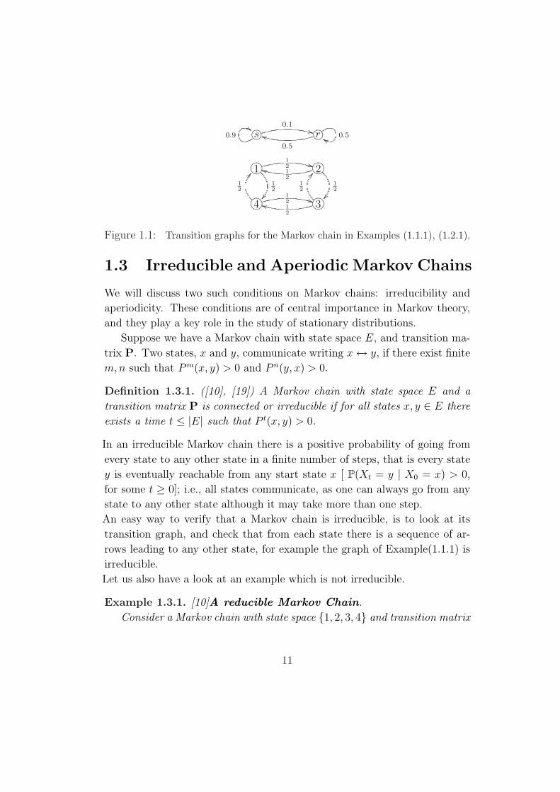
Figure 1.1: Transition graphs for the Markov chain in Examples (1.1.1), (1.2.1).

1.3 Irreducible and Aperiodic Markov Chains

We will discuss two such conditions on Markov chains: irreducibility and

aperiodicity. These conditions are of central importance in Markov theory,

and they play a key role in the study of stationary distributions.

Suppose we have a Markov chain with state space E, and transition ma-

trix P. Two states, x and y, communicate writing x ↔ y, if there exist finite

m,n such that Pm(x, y) > 0 and P n(y, x) > 0.

Definition 1.3.1. ([10], [19]) A Markov chain with state space E and a

transition matrix P is connected or irreducible if for all states x, y ∈ E there

exists a time t ≤ |E| such that P t(x, y) > 0.

In an irreducible Markov chain there is a positive probability of going from

every state to any other state in a finite number of steps, that is every state

y is eventually reachable from any start state x [ P(Xt = y | X0 = x) > 0,

for some t ≥ 0]; i.e., all states communicate, as one can always go from any

state to any other state although it may take more than one step.

An easy way to verify that a Markov chain is irreducible, is to look at its

transition graph, and check that from each state there is a sequence of ar-

rows leading to any other state, for example the graph of Example(1.1.1) is

irreducible.

Let us also have a look at an example which is not irreducible.

Example 1.3.1. [10]A reducible Markov Chain.

Consider a Markov chain with state space 1, 2, 3, 4 and transition matrix

11

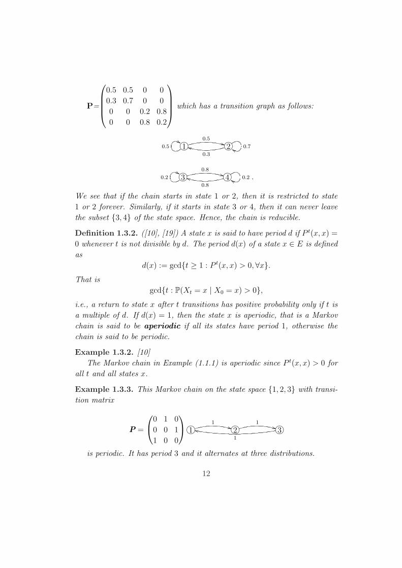
P=

0.5 0.5 0 0

0.3 0.7 0 0

0 0 0.2 0.8

0 0 0.8 0.2

which has a transition graph as follows:

/.-,()*+10.5%% 0.5

**/.-,()*+2 0.7ee0.3

jj

/.-,()*+30.2%% 0.8

**/.-,()*+4 0.2ee0.8

jj .

We see that if the chain starts in state 1 or 2, then it is restricted to state

1 or 2 forever. Similarly, if it starts in state 3 or 4, then it can never leave

the subset 3, 4 of the state space. Hence, the chain is reducible.

Definition 1.3.2. ([10], [19]) A state x is said to have period d if P t(x, x) =

0 whenever t is not divisible by d. The period d(x) of a state x ∈ E is defined

as

d(x) := gcdt ≥ 1 : P t(x, x) > 0, ∀x.That is

gcdt : P(Xt = x | X0 = x) > 0,i.e., a return to state x after t transitions has positive probability only if t is

a multiple of d. If d(x) = 1, then the state x is aperiodic, that is a Markov

chain is said to be aperiodic if all its states have period 1, otherwise the

chain is said to be periodic.

Example 1.3.2. [10]

The Markov chain in Example (1.1.1) is aperiodic since P t(x, x) > 0 for

all t and all states x.

Example 1.3.3. This Markov chain on the state space 1, 2, 3 with transi-

tion matrix

P =

0 1 0

0 0 1

1 0 0

/.-,()*+1

1**/.-,()*+2

1**/.-,()*+3

1

ll

is periodic. It has period 3 and it alternates at three distributions.

12

The transition graph of the Markov chain in Example (1.2.1) has period

d = 2, since a particle can return to each state after 2, 4, 6, . . . steps.

Lemma 1.3.1. If the states x and y communicate, and if x has period d,

then so has state y.

This means that the state x is aperiodic if x ↔ y and P (y, y) > 0.

One reason for the usefulness of aperiodicity is the following theorem.

Theorem 1.3.1. [10] Suppose that we have an aperiodic Markov chain X0, X1, . . . with state space E and transition matrix P. Then there exists an T < ∞ such

that

P t(x, x) > 0

for all x ∈ E and all t ≥ T.

By combining aperiodicity and irreducibility, we get the following im-

portant corollary, which will be used to prove the so-called Markov chain

convergence theorem, see Theorem 3.2.1.

Corollary 1.3.1. [10] Now suppose our Markov chain is aperiodic and irre-

ducible. Then there exist an T < ∞ such that

P t(x, y) > 0

for all x, y ∈ E and all t ≥ T.

1.4 Important Properties of Markov Chains

In the following section we will summarize some of the most common prop-

erties of Markov chains that are used in the context of MCMC. We always

refer to a Markov chain X0, X1, X2, . . . with transition matrix P on a finite

state space E.

Given an initial state X0 = x of a Markov chain with transition matrix

P, the probability of first return to state x at time t is given by

f t(x, x) = P(Xt = x, and for 1 ≤ s ≤ t− 1, Xs 6= x|X0 = x)

13

and for x 6= y,

f t(x, y) = P(Xt = y, and for 1 ≤ s ≤ t− 1, Xs 6= y|X0 = x)

is the probability of first arrival at state y at time t, (i.e., first transition into

state y occurs at time t).

For each x ∈ E, let

f(x, x) =∞∑

t=1

f t(x, x)

be the probability that leaves state x sooner or later, return to that state,

(i.e., there is a transition into state x at some time t > 0).

In other words, f(x, x) = P(T < ∞), where T = inft ≥ 1 : Xt = x is the

number of steps for reaching state x for the first time known as the hitting

time with T = ∞ if no such time exists.

The expected number of time steps to reach state y starting at x is

h(x, y) =∞∑

t=1

tf t(x, y).

Definition 1.4.1. [19] A state, x, is a recurrent state if f(x, x) = 1.

It is called transient if f(x, x) < 1, and therefore h(x, x) = ∞. Thus,

x is a transient state if given that we start in state x, there is a non-zero

probability that we will never return back to x. Positive recurrent means

that the expected return time is finite for every state.

Lemma 1.4.1. [19]

(a) The state x is recurrent if and only if∞∑

t=1

P t(x, x) = ∞.

(b) If state y is transient, then∞∑

t=1

P t(x, y) < ∞.

Theorem 1.4.1. [3]If x is recurrent and P (x, y) > 0, then y is recurrent

and P (y, x) = 1.

14

A simple example of Markov chain with two recurrent classes [a class

will be called recurrent, if all (one) of the states are (is) recurrent] can be

represented by transition matrix of Example (1.3.1), since states 1 ↔ 2 but

neither state 1 nor state 2 communicates with state 3 or 4.

Example 1.4.1. Here is a Markov chain on state space E = x1, x2, x3,with transition matrix

P =

0 1 012

0 12

0 1 0

76540123x1

1++ 76540123x2

12

kk

12

++ 76540123x3

1

kk .

The transition graph of this Markov chain has three recurrent states, and

one recurrent class.

Note: Sometimes the terms indecomposable, a cyclic, and persistent are

used as synonyms for “irreducible”, “aperiodic”, and “recurrent” respectively.

Example 1.4.2. Consider the Markov chain with state space 0, 1, 2, 3, 4and transition matrix

P =

0 13

0 0 23

0 0 14

34

012

0 0 0 12

0 0 0 0 1

0 0 0 35

25

.

Since P (4, 4) > 0 and states 3 and 4 communicate, it follows from Lemma

(1.3.1) that these states are aperiodic. State 0 has period 3. From 0 the chain

moves to either 1 or 4. From 4 it never moves back to 0 while from 1 the

chain moves to either 2 or 3. From 3 it never moves back to 0. From 2 it

moves to either 0 or 4. This shows that 0 is transient and that P n(0, 0) > 0

only if n is a multiple of 3. As a result, the transient state 0 has period 3.

Since 0 ↔ 1 ↔ 2. By Lemma (1.3.1) the states 1 and 2 also have period

3. P (4, 3) > 0 and P (3, 4) = 1 so 4 must be recurrent, but P (1, 3) > 0 and

P (3, 1) = 0 so 1 must be transient, or we would contradict Theorem (1.4.1).

15

In the context of MCMC a question of particular interest is the question

of the long-term behavior of a Markov chain. Given certain conditions, does

the distribution of the chain converge to a well defined and unique limit?.

The concept of irreducibility and aperiodicity will provide an answer.

1.5 Stationary Distributions

We consider one of the central issues in Markov theory: asymptotic for the

long-term behavior of Markov chains.

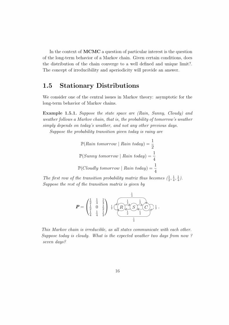
Example 1.5.1. Suppose the state space are (Rain, Sunny, Cloudy) and

weather follows a Markov chain, that is, the probability of tomorrow’s weather

simply depends on today’s weather, and not any other previous days.

Suppose the probability transition given today is rainy are

P(Rain tomorrow | Rain today) =1

2

P(Sunny tomorrow | Rain today) =1

4

P(Cloudly tomorrow | Rain today) =1

4

The first row of the transition probability matrix thus becomes (12, 1

4, 1

4).

Suppose the rest of the transition matrix is given by

P =

12

14

14

12

0 12

14

14

12

GFED@ABCR1

2

++14 **

@GF ED14

²²GFED@ABCS

12

kk

12 ++GFED@ABCC14

jj12kkBCD@GA

14

??.

This Markov chain is irreducible, as all states communicate with each other.

Suppose today is cloudy. What is the expected weather two days from now ?

seven days?

16

Here P 0 =(0 0 1

). Hence

P 2 = P 0P2 = (001)

12

14

14

12

0 12

14

14

12

12

14

14

12

0 12

14

14

12

=(0 0 1

)

716

316

38

38

14

38

38

316

716

=(

38

316

716

)

=(0.375 0.1875 0.4375

),

and

P 7 = P 0P7 =(

8192048

8194096

16394096

)

=(0.3999 0.1999 0.4001

)

=(0.4 0.2 0.4

).

Conversely, suppose today is rainy, so that P 0 =(1 0 0

).

The expected weather becomes

P 2 =(1 0 0

)

716

316

38

38

14

38

38

316

716

=(

716

316

38

)

=(0.4375 0.1875 0.375

),

and P 7 =(0.4 0.2 0.4

).

After a sufficient amount of time, the expected weather is independent of

the starting value. In other words, the chain has reached a stationary distri-

bution, where the probability values are independent of the actual starting

value. The previous example illustrates, a Markov chain may reach a station-

ary distribution π, where the vector of probabilities of being in any particular

given state is independent of the initial condition.

Example 1.5.2. Consider the Markov chain on state space E = 0, 1, 2with the transition matrix

17

P=

13

13

13

0 1 0

0 0 1

. Then Pt=

13t

1−3−t

21−3−t

2

0 1 0

0 0 1

t→∞−−−→

0 12

12

0 1 0

0 0 1

,

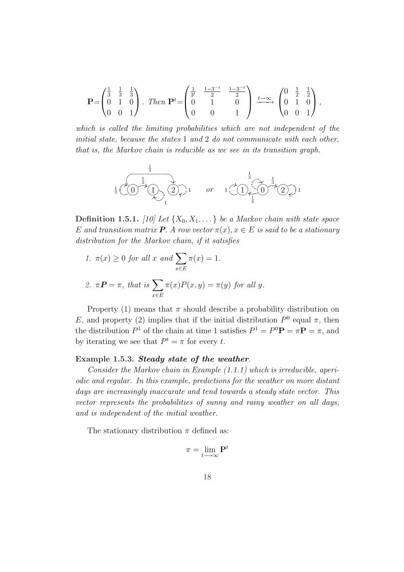
which is called the limiting probabilities which are not independent of the

initial state, because the states 1 and 2 do not communicate with each other,

that is, the Markov chain is reducible as we see in its transition graph.

?>=<89:;013

))13 **

@GF ED13

²²?>=<89:;1

1

TT?>=<89:;2 1ii or ?>=<89:;11

)) ?>=<89:;0

13

··

13

jj

13 ** ?>=<89:;2 1ii

Definition 1.5.1. [10] Let X0, X1, . . . be a Markov chain with state space

E and transition matrix P. A row vector π(x), x ∈ E is said to be a stationary

distribution for the Markov chain, if it satisfies

1. π(x) ≥ 0 for all x and∑x∈E

π(x) = 1.

2. πP = π, that is∑x∈E

π(x)P (x, y) = π(y) for all y.

Property (1) means that π should describe a probability distribution on

E, and property (2) implies that if the initial distribution P 0 equal π, then

the distribution P 1 of the chain at time 1 satisfies P 1 = P 0P = πP = π, and

by iterating we see that P t = π for every t.

Example 1.5.3. Steady state of the weather.

Consider the Markov chain in Example (1.1.1) which is irreducible, aperi-

odic and regular. In this example, predictions for the weather on more distant

days are increasingly inaccurate and tend towards a steady state vector. This

vector represents the probabilities of sunny and rainy weather on all days,

and is independent of the initial weather.

The stationary distribution π defined as:

π = limt−→∞

Pt

18

but only converges if P is a regular transition matrix (that is, there is at

least one P t with all non-zero entries). For the weather example:

P =

(0.9 0.1

0.5 0.5

).

And since πP = π [π is unchanged byP].

Then π[P− I] = 0

= π

[(0.9 0.1

0.5 0.5

)−

(1 0

0 1

)]

= π

(−0.1 0.1

0.5 −0.5

).

Therefore(π(1) π(2)

) (−0.1 0.1

0.5 −0.5

)=

(0 0

).

So

−0.1π(1) + 0.5π(2) = 0 and since they are a probability vector we know

that

π(1) + π(2) = 1. Solving this pair of simultaneous equations gives the

steady state distribution:

(π(1) π(2)

)=

(0.833 0.167

).

In conclusion, in the long term, 0.83 of days are sunny.

Example 1.5.4. Markov chains are used in the study of probabilities con-

nected to genetic models. Genes come in pairs; and for any trait governed

by a pair of genes, an individual may have genes of the gene type GG (dom-

inant), Gg (hybrid), or gg (recessive). Each offspring inherits one gene from

one parent, at random and independently.

1. Suppose that an individual of unknown genetic makeup is matched with

a hybrid. Set up a transition matrix to describe the possible states of

a resulting offspring and their probabilities.

2. What will happen to the genetic makeup of the offspring after many

generations of matching with a hybrid?

19

Solution: If the unknown is dominant (GG) and is matched with a hybrid

(Gg), the offspring has a probability of 12

of being dominant and a probability

of 12

of being hybrid. If two hybrids are matched, the offspring may be

dominant, hybrid or recessive with probabilities 14, 1

2, and 1

4, respectively. If

the unknown is recessive (gg), the offspring of it and a hybrid has probability12

of being recessive and a probability of 12

of being hybrid. So, a transition

matrix from the unknown parent to an offspring is given by

P =

12

12

014

12

14

0 12

12

,

where the states are E = d, h, r. Since the matrix P2 has all positive

entries, and hence a stationary distribution π = (π(1), π(2), π(3)) exists.

From the matrix equation

π = πP

along with π(1) + π(2) + π(3) = 1 we obtain

π = (1

4,1

2,1

4).

No matter what the genetic makeup of the unknown parent happens to be,

the ratio to dominant to hybrid to recessive offspring among its descendants,

after many generations of mating with hybrids, should be 1 : 2 : 1.

Definition 1.5.2. A Markov chain is ergodic if it is both irreducible and

aperiodic.

Example 1.5.5. The Markov chain on state space E = 0, 1, 2 with tran-

sition matrix

P =

12

0 12

13

13

13

0 1 0

?>=<89:;01

2

))@GF ED

12

²²?>=<89:;1

13jj

13 **

13

TT?>=<89:;2BCD@GA

1

??

is an ergodic since it is irreducible and aperiodic.

20

Definition 1.5.3. A Markov chain X0, X1, X2, . . . is called ergodic if the

limit

π(y) = limt−→∞

P t(x, y)

(1) exists for all y ∈ E

(2) is positive and does not depend on x

(3) π(x), x ∈ E is a probability distribution on E.

Ergodic Markov chain are useful for convergence theorem:

Theorem 1.5.1. [10]Existence of stationary distribution.

For any irreducible and aperiodic Markov chain, there exists at least one

stationary distribution.

1.6 Detailed Balance and Time Reversal

We are interested in constructing Markov chains for which the distribution

we wish to sample from, given by π, is invariant (stationary), so we need to

find transition matrices P that satisfies π = πP. That is, if P (x, y) denotes

the probability of a transition from x ∈ E to y ∈ E under P, we require that∑x

π(x)P (x, y) = π(y) for all y. We introduced a special class of Markov

chains known as the reversible ones.

Definition 1.6.1. A stationary Markov chain X0, X1, X2, . . . : Ω −→ E

with transition matrix P and stationary distribution π is called reversible

if its finite-dimensional distributions do not depend on the orientation of

the time axis, i.e., if P(X0 = x0, X1 = x1, . . . , Xt−1 = xt−1, Xt = xt)=

P(Xt = x0, Xt−1 = x1, . . . , X1 = xt−1, X0 = xt) for arbitrary t ≥ 0 and

x0, . . . , xt ∈ E.

The reversibility of Markov chains is a particularly useful property for

the construction of dynamic simulation algorithms, see Section (4.2).

21

Definition 1.6.2. [10] A probability distribution π on the state space E is

reversible for the Markov chain X0, X1, . . . with transition matrix P if for

all x, y ∈ E we have

π(x)P (x, y) = π(y)P (y, x),

which is also known as detailed balance equation.

Definition 1.6.3. A Markov chain with state space E = Z is called a random

walk if, for some number p ∈ (0, 1) we have

P (x, x + 1) = p and P (x, x− 1) = 1− p for x ∈ E.

We can call it a random walk because we may think of it as being a model for

an individual walking on a straight line who at each point of time either takes

one step to the right with probability p or one step to the left with probability

1− p.

Example 1.6.1. [10] Consider a “random walk” on the vertices of a graph

G = (V, E)(a square) consists of a vertex set V together with an edge set E.

Each edge connects two of the vertices; an edge connecting the vertices vi and

vj is denoted (vi, vj). No two edges are allowed to connect the same pair of

vertices. Two vertices are said to be neighbours if they share an edge.

This random walk is a Markov chain with state space V = v1, v2, v3, v4and here E = (v1, v2), (v2, v3), (v3, v4), (v4, v1).

v1• •v2

v4• •v3

If we denote the number of neighbours of a vertex vi by di, then the elements

of the transition matrix are given by

P (i, j) =

1di

= 12

if vi and vj are neighbours

0 otherwise,(1.6.1)

22

which is a reversible Markov chain, with reversible distribution π given by

π =

(d1

d, . . . ,

d4

d

)=

(1

4,1

4,1

4,1

4

),

where d =4∑

i=1

di since it satisfies detailed balance equation. To see that, we

calculate

π(i)P (i, j) =

di

d1di

= 1d

= 18

=dj

d1dj

= π(j)P (j, i) if vi and vj are neighbours

0 = π(j)P (j, i) otherwise.

It is possible for a distribution to be stationary without detailed balance

holding.

Example 1.6.2. A nonreversible Markov chain.

Let X1, . . . , Xt be the Markov chain in Example (1.3.3), then the uni-

form distribution π = (13, 1

3, 1

3) on the state space 1, 2, 3 is stationary (in-

variant) but detailed balance does not hold, to see this: let x = 1, y = 2, we

get

π(1)P (1, 2) =1

3.1 =

1

3> 0 =

1

3.0 = π(2)P (2, 1),

so that π(1)P (1, 2) 6= π(2)P (2, 1) and reversibility fails.

Also, if we let X0 = 1, then Xt = 1 whenever t = 0, 3, 6, 9, ...( a multiple

of 3), thus P(Xt = 1) = 0 or 1, so P(Xt = 1) 6−→ π(3), and there is again

no convergence to π.

Example 1.6.3. The following example is not reversible. Let E = 1, 2, 3, 4and

P =

0 34

0 14

14

0 34

0

0 14

0 34

34

0 14

0

/.-,()*+134 **

14

¢¢

/.-,()*+214

jj

34

¢¢/.-,()*+4

34

AA

14 **/.-,()*+334

jj

14

AA .

The transition matrix P is irreducible, but not aperiodic, and stationary

distribution (which is uniquely determined by Definition (1.5.1)) is given by

23

π = (14, 1

4, 1

4, 1

4). However,

π(1)P (1, 2) =1

4.3

4=

3

16>

1

16=

1

4.1

4= π(2)P (2, 1).

This cyclic random walk is not reversible as clockwise steps are much more

likely than counterclockwise movements.

The next simple theorem will help us in constructing MCMC algorithms

that (approximately) sample from a given distribution π.

Theorem 1.6.1. [10]Detailed Balance Test.

If the probability distribution π is reversible for a Markov chain, then it is

also a stationary distribution for the chain.

Proof. Since π is reversible, we have ∀ x, y,

π(x)P (x, y) = π(y)P (y, x).

For fixed x ∈ E, we sum this equation with respect to y ∈ E to get

∑y

π(x)P (x, y) =∑

y

π(y)P (y, x).

But the left hand side equals π(x)∑

y

P (x, y) = π(x), since rows sum to one.

Thus, ∀ x, y,

π(x) =∑

y

π(y)P (y, x),

and this implies π = πP, which makes π a stationary distribution.

If a Markov chain satisfies the detailed balance condition, then it is time

reversible, i.e., one could not tell whether a sequence of samples is being ac-

quired forward or backward in time. That is, at stationarity, the probability

of transition being from state x to state y is the same as the probability of

it being from state y to state x.

24

Chapter 2

Markov Chain Monte Carlo

Algorithms

It is often difficult to sample directly from the distribution π; the reason is

that they are defined as π(x) = f(x)z

, where f(x) is an easily computable

density function, and z is unknown normalizing constant that is often very

difficult to compute. In such circumstance we can use algorithms (Markov

Chain Monte Carlo MCMC simulation) that help us with sampling from

complicated and high dimensional distributions, so the method of simulating

a Markov chain whose stationary distribution is the distribution we want to

sample from is known in general as Markov Chain Monte Carlo.

MCMC method is a class of algorithms for sampling from probability distri-

butions based on constructing a Markov chain X0, X1, X2, . . . having state

space E and has the desired (target) distribution as its stationary distribution

π. When used in MCMC algorithms, Markov chains are usually constructed

from a Markov transition kernel P, a conditonal probability density on E such

that Xt+1|Xt ∼ P (Xt, Xt+1). As we saw in Section 1.2, ∀ x ∈ E, P (x, y) rep-

resents the probability of moving from x to y, and P t(x, y) is the probability

that the Markov chain with initial state x is in state y after t iterations. The

transition kernel must satisfy P t(x, y) −→ π as t −→∞, for all initial states

x.

Now suppose we want to draw a sample from a density distribution π.

The main idea behind MCMC is to start from an arbitrary state in E, run a

25

Markov chain, whose stationary distribution equals to π, for a long time, say

t iterations, and note what state the chain is in after these t iterations, and

then take the result“output” as an approximate sample from π. The ergodic-

ity means that, by taking t large enough, we can ensure that the distribution

of the output state is arbitrarily close to the desired distribution π. So if

the Markov chain has reached equilibrium, the output is distributed accord-

ing to the stationary distribution, as desired. MCMC techniques provide a

powerful tool for statistical analysis for data.

In this chapter, we construct Markov chains with the required station-

ary distribution by presenting two common techniques which have ignited

MCMC: The Metropolis-Hastings algorithms and the Gibbs sampler.

2.1 Metropolis Algorithm

The classic paper of Metropolis et al. [15], was the first to use Markov chain

sampling, in the form now known as the Metropolis algorithm. This algo-

rithm has since been applied extensively to problems in statistical physics.

The Metropolis algorithm, was born in 1953, uses a symmetric candidate

generating distribution (a transition matrix Q = q(x, y)) on E for which

q(x, y) = q(y, x). Suppose our goal is to draw samples from some distribu-

tion π(x) where π(x) = f(x)z

, such that the normalizing constant z may not

be known, and very difficult to compute.

Define a Markov chain with the following process:

(1) Start with any initial value x0 satisfying f(x0) > 0.

(2) Using current value xt, sample a candidate point x∗ from a symmetric

candidate distribution q(x, y) which is the probability of returning a

value of y given a previous value of x.

(3) Calculate the ratio r of the density at the candidate x∗ and current point

xt (this is easy since the normalization constant z cancels)

r =π(x∗)π(xt)

=f(x∗)

zf(xt)

z

.

26

(4) If the above calculation gives (r > 1), accept the candidate point (set

xt+1 = x∗), and return to step 2.

In detail, this can be done by generating a random number, U, from

the uniform distribution on [0, 1], and then sitting the next state as

follows:

xt+1 =

x∗ if U < α(xt, x∗)

xt otherwise.(2.1.1)

This generates a Markov chain x0, x1, . . . , xk, . . . as the transition proba-

bilities from xt to xt+1 depends only on xt and not on x0, . . . , xt−1.

Following a sufficient burn-in period (of k steps), the chain approaches its

stationary distribution and samples from xk+1, . . . , xk+m are samples from

π(x).

Example 2.1.1. Consider the scalar inverse χ2 distribution,

π(x) = C.x−n2 exp

(−a

2x

)(2.1.2)

and suppose we wish to simulate draws from the distribution with (n = 5)

degrees of freedom, and scaling factor a = 4 using the Metropolis algorithm.

Suppose that a uniform distribution on [0, 100] is the candidate distribution.

Take x0 = 1 as starting (initial) value, and suppose the uniform returns a

candidate value of x∗ = 39.82. Here

α = min(r, 1) = min

(f(x∗)f(xt)

, 1

)= min

((39.82)−2.5 exp( −2

39.82)

(1)−2.5 exp(−21

), 1

)= 0.0007

α = 0.0007 < 1, implies x∗ is accepted with probability 0.0007.

Thus, we randomly draw U from a uniform [0, 1] and accept x∗ if U ≤ α.

In this case, the candidate is rejected, and we draw another candidate value

from the candidate distribution (which turns out to be 71.36), then

α = min

((71.36)−2.5 exp( −2

71.36)

(1)−2.5 exp(−21

), 1

)= 0.0002 < 1,

implies 71.36 is accepted with probability 0.0002, and continue as above for

(say) 500 values of x.

27

2.2 Metropolis-Hastings Algorithm

If we want to sample from some distribution π that has a sample space

of high dimension, then we want a Markov chain whose unique stationary

distribution is π, and run this chain long enough and then take the result

as an approximate sample from π. A very general way to construct such

a Markov chain is the Metropolis-Hastings algorithm. Since the symmetry

requirement of the Metropolis proposal distribution can be hard to satisfy,

Hastings in (1970)[11] extended the Metropolis algorithm to a more general

candidate transition which converges to π(x) by using an arbitrary transition

probability function q(x, y) = P(x −→ y), (i.e., a Markov transition kernel).

The algorithm proposes a new point (state) on the Markov chain which

is either accepted or rejected.

• If the state is accepted, the Markov chain moves to the new state.

• If the state is rejected, the Markov chain remains in the same state.

By choosing the acceptance probability correctly, we create a Markov chain

which has π as a stationary distribution. We begin with a state space E and

a probability distribution π on E. Then we choose a candidate distribution

q(x, y) : x, y ∈ E with q(x, y) ≥ 0 and∑

y

q(x, y) = 1 for each x ∈ E.

The algorithm works as follows:

(1) Sample a candidate point “ state” x∗ from the candidate distribution

q(x, y) which is not necessarily symmetric.

(2) Compute the ratio r =π(x∗)q(x∗, xt)

π(xt)q(xt, x∗).

(3) With probability α(xt, x∗) = min(r, 1), transition to x∗ “ accept the can-

didate” . Otherwise, stay in the same state xt “ reject the candidate”,

where

α(xt, x∗) =

min(r, 1) if π(xt)q(xt, x∗) > 0

1 if π(xt)q(xt, x∗) = 0.(2.2.1)

28

(4) Discard initial “ burn in” values.

(5) Remaining x′s are ∼ independent and identically distribution (i.i.d.)

π(x).

The initial value is arbitrarily selected, which means Metropolis-Hastings

typically has “ burn in” period at the start of a simulation.

Now for reversible chains it is impossible to distinguish between forward

and backward running of the chain. So, to construct the transition probabil-

ities P (x, y), we set

P (x, y) = q(x, y)α(x, y), (2.2.2)

where q(x, y)’s are the transition probabilities for another Markov chain ful-

filling

q(x, y) > 0 =⇒ q(y, x) > 0 ∀ x, y ∈ E. (2.2.3)

Finally, to see why the Metropolis-Hastings algorithm work (generates a

Markov chain whose equilibrium density is that candidate density f(x)), it is

sufficient to show that the implied transition kernel q(x, y) of any Metropolis-

Hastings algorithm satisfies the detailed balance equation, i.e., we want to

show that the Markov chain resulting from the Metropolis-Hastings algorithm

is reversible with respect to π.

Theorem 2.2.1. [4] The Metropolis-Hastings algorithm produces a Markov

chain X0, X1, . . . which is reversible with respect to π.

Proof. We must show that π(x)P (x, y) = π(y)P (y, x).

Obviously this holds if x = y, so we will consider x 6= y, then

π(x)P (x, y) = π(x)q(x, y)α(x, y)

= π(x)q(x, y) min

1,

π(y)q(y, x)

π(x)q(x, y)

= minπ(x)q(x, y), π(y)q(y, x). (2.2.4)

Similarly, we find that

π(y)P (y, x) = minπ(x)q(x, y), π(y)q(y, x).

29

This implies that

π(x)P (x, y) = π(y)P (y, x).

Therefore, the chain is reversible.

It follows that the Metropolis-Hastings algorithm converges to the target

distribution π which is the stationary distribution by detailed balance.

Example 2.2.1. If x has a χ2 distribution with n degrees of freedom, short-

hand notation for this x ∼ χ2n, then the pdf of x is given by

f(x) =

1

Γ(n2)2

n2x(n

2)−1e

−x2 if x > 0

0 otherwise.(2.2.5)

Now suppose we wish to use a χ2 distribution as our candidate density, by

simply drawing from a χ2 distribution independent of the current position.

Thus, q(x, y) = f(y) =1

Γ(n2)2

n2

y(n2)−1e

−y2 which implies that q(x, y) is not

symmetric, since q(x, y) = f(y) 6= f(x) = q(y, x). Hence, we must use the

Metropolis-Hastings sampling, with acceptance probability

α(x, y) = min

(π(y)q(y, x)

π(x)q(x, y), 1

)= min

(π(y)x(n

2)−1e

−x2

π(x)y(n2)−1e

−y2

, 1

),

move to y, otherwise stay at x.

Using the target distribution as in (2.1.2),

π(x) = C.x−52 exp

(−2

x

),

the rejection probability becomes

α(x, y) =

min

[y−52 exp(−2

y )x( n2 )−1e

−x2

x−52 exp(−2

x )y( n2 )−1e

−y2

, 1

]if π(x)q(x, y) > 0

1 if π(x)q(x, y) = 0.

(2.2.6)

30

2.3 The Gibbs Sampler

Gibbs sampling is a statistical method that allows us to generate random vari-

ables from highly complicated distributions without calculating their density

functions. Gibbs sampling was introduced by [15]. Later, the approach was

modified and improved by [11]. A good introduction into Gibbs sampling

can be found in [2]. One of the first applications of Gibbs sampling is shown

in [8], where it is used for the digital restoration of images.

The Gibbs sampler introduced by Geman and Geman [8], also known as the

Heat Bath Algorithm for simulating a Markov chain X0, X1, . . . which

is converging to the target distribution π(x), by successively sampling from

the full conditional component distribution π(xi | x−i), i = 1, . . . , n, where

x−i denotes the components of x other than xi. The idea behind the Gibbs

sampler is that one only considers univariate conditional distributions-the

distribution when all of the random variables but one are assigned fixed val-

ues. Such conditional distributions are far easier to simulate than complex

joint distributions and usually have simple forms often being normals, or in-

verse χ2. The Gibbs sampler is a method for generating samples from the

joint distribution of two or more variables and it is a special case of the

Metropolis-Hastings algorithm where the proposals q (the candidate distri-

butions) are the full conditionals and the acceptance probability is always

1.

To show this let the candidate distribution be

q(x, y) =

π(yi | x−i) if y−i = x−i

0 otherwise.(2.3.1)

31

The importance ratio is

r =π(y)q(y, x)

π(x)q(x, y)

=π(y)π(xi | y−i)

π(x)π(yi | x−i)Definition of the candidate distribution

=π(y)π(xi | x−i)

π(x)π(yi | y−i)

=π(y)π(xi, x−i)π(y−i)

π(x)π(yi, y−i)π(x−i)Definition of conditional probability

=π(y−i)

π(x−i)= 1. We did not change other variables.

(2.3.2)

So the acceptance probability is α(x, y) = min

(1,

π(y)π(xi|x−i)

π(x)π(yi|y−i)

)= 1.

This means that the Gibbs sampler is the best, since the candidate is

always accepted.

Let π(X) be the joint distribution of X = (X1, . . . , Xn), and let π(Xi |X−i) = π(Xi | X1, . . . , Xi−1, Xi+1, . . . , Xn) be the pdf for Xi given all other

components. These distributions are called the full conditionals. To use the

Gibbs sampler, the marginal distribution of all the variables must be known.

Now for simplicity consider the case when n = 2.

The Gibbs sampler generates a Markov chain (X1, Y1), (X2, Y2), . . . , (Xk, Yk)converging to π(X, Y ), by successively sampling

X1 from π(X | Y0)

Y1 from π(Y | X1)

X2 from π(X | Y1)...

Xk from π(X | Yk−1)

Yk from π(Y | Xk).To get started, prespecify an initial value for Y0.

32

Example 2.3.1. [2] Suppose the joint distribution of x = 0, 1, ..., n which is

discrete, and 0 ≤ y ≤ 1 which is continuous is given by

f(x, y) =n!

(n− x)!x!

Γ(α + β)

Γ(α)Γ(β)yx+α−1(1− y)n−x+β−1,

where the joint density is complex.

The Gibbs sampler, having f as its stationary distribution proceeds by suc-

cessively sampling from the conditional distributions X|y ∼ b(n, y), and the

conditional density y|x ∼ Beta(x+α, n−x+β). To see this, first recall that

a binomial random variable z has a density function

f(z|p, n) =n!

(n− z)!z!pz(1− p)n−z for z = 0, 1, 2, . . . , n,

where 0 < p < 1 is the success parameter and n is the number of trails, and

we denote z ∼ b(n, p).

Likewise recall the density for z ∼ Beta(a, b), a beta distribution with shape

parameters a and b is given by

f(z|a, b) =Γ(a + b)

Γ(a)Γ(b)za−1(1− z)b−1 for 0 ≤ z ≤ 1.

The marginal distribution of x is given by

f(x) = P(X = x) =

1∫

0

f(x, y)dy =

1∫

0

n!

(n− x)!x!

Γ(α + β)

Γ(α)Γ(β)yx+α−1(1− y)n−x+β−1dy

=n!

(n− x)!x!

Γ(α + β)

Γ(α)Γ(β)

1∫

0

yx+α−1(1− y)n−x+β−1dy

=n!

(n− x)!x!

Γ(α + β)

Γ(α)Γ(β)

Γ(x + α)Γ(n− x + β)

Γ(α + β + n).

Which is called the beta-binomial (n, α, β).

33

And the marginal distribution of y is given by

f(y) = P(Y = y) =n∑

x=0

f(x, y) =n∑

x=0

n!

(n− x)!x!

Γ(α + β)

Γ(α)Γ(β)yx+α−1(1− y)n−x+β−1

=Γ(α + β)

Γ(α)Γ(β)yα−1(1− y)β−1

n∑x=0

n!

(n− x)!x!yx(1− y)n−x

=Γ(α + β)

Γ(α)Γ(β)yx(1− y)n−x.1

=Γ(α + β)

Γ(α)Γ(β)yx(1− y)n−x.

Hence, y ∼ Beta(α, β).

With these probability distributions, the conditional distribution of x ( y is

a fixed constant) is

f(X|y) =f(x, y)

f(y)

=

n!(n−x)!x!

Γ(α+β)Γ(α)Γ(β)

yx+α−1(1− y)n−x+β−1

Γ(α+β)Γ(α)Γ(β)

yα−1(1− y)β−1

=n!

(n− x)!x!yx(1− y)n−x.

Thus, X|y ∼ b(n, y). While

f(y|x) =f(x, y)

f(x)

=

n!(n−x)!x!

Γ(α+β)Γ(α)Γ(β)

yx+α−1(1− y)n−x+β−1

n!(n−x)!x!

Γ(α+β)Γ(α)Γ(β)

Γ(x+α)Γ(n−x+β)Γ(α+β+n)

=Γ(α + β + n)

Γ(x + α)Γ(n− x + β)yx+α−1(1− y)n−x+β−1.

Therefore, y|x ∼ Beta(x + α, n− x + β).

To illustrate the Gibbs sampler for the above, suppose n = 10 and α = 1, β = 2.

The algorithm of the sampler is as follows:

34

(1) Start with some initial value y0 = Beta(α, β) = Beta(1, 2) = Γ(1)Γ(2)Γ(3)

=0!1!2!

= 12

for y and obtain X0 by generating a random variable from

the conditional distribution X|y = y0 = 12∼ b(n, y0) = b(10, 1

2), giving

X0 = 5 in our simulation.

(2) Use x0 = 5 to generate a new value of y1, drawing from the conditional

distribution y|x = 5 ∼ Beta(x0+α, n−x0+β) = Beta(5+1, 10−5+2) =

Beta(6, 7) based on the value x0 = 5, giving y1 = 0.33.

(3) Repeat step (1) to obtain X1 = 3 which is a realisation of b(n, y1) =

b(10, 0.33) random variable.

(4) Repeat step (2) to obtain y2 = 0.56 from Beta(x1 + α, n − x1 + β) =

Beta(3 + 1, 10− 3 + 2) = Beta(4, 9).

(5) Similarly X2 = 7 is obtained from b(n, y2) = b(10, 0.56) random variable.

Thus, after repeating this process three times “iterations”, we generate a

Gibbs sequence “a Markov chain” of length k = 3, where a subset of points

(5, 0.5), (3, 0.33), (7, 0.56) are taken as our simulated draws from the full joint

distribution.

Remark 2.3.1. Note that, the initial values in the chain (the Gibbs sequence)

are dependent on the y0 value chosen to start the chain. This dependence

decays as the sequence length increases and so we typically start after a suf-

ficient number of “burn-in” iterations have occurred to remove any effects of

the starting conditions (initial sampling values).

The Gibbs sequence converges to a stationary (equilibrium) distribution

that is independent of the starting values, and by construction this stationary

distribution is the target distribution we are trying to simulate [23].

Remark 2.3.2. As we have seen, we use the Gibbs sampler and the Metropolis-

Hastings algorithms to simulate a Markov chain X1, . . . , Xk which converges

in distribution to π(X), [i.e., as k increases, the distribution of Xk gets closer

and closer to π(X)]. Simulation of a Markov chain requires a starting value

X0 such that if the chain is converging to π(X), then the dependence between

say Xj and X0 diminishes as j increases. After a suitable “burn in” period

of N iterations, XN , . . . , Xk behaves like a dependent sample from π(X).

35

Chapter 3

Coupling

A fundamental problem of MCMC algorithms is the determination

of the number of iterations required, so that the result will be approximately

a sample from the distribution of interest.

Recently, a new variant of MCMC method, which is called perfect sim-

ulation algorithms, have been developed. These are algorithms which au-

tomatically ensure that the Markov chain is only sampled after equilibrium

has been reached. The basis of perfect simulation are couplings. The cou-

pling method, deals with comparison of probability measures on a measurable

space. It is an important tool in probability theory and its applications, is

primarily used in estimates of total variation distances. The method also

works well in establishing inequalities and has been highly successful in the

study of Markov chain.

In this chapter, we will discus how to couple paths of a Markov chain

which are started in different initial states.

3.1 Convergence in Variation and Coupling

Let µ and ν be two probability distributions on a finite state space E. That

is, µ(x)= probability that x occurs. A distribution ω on E×E is a coupling

if:

36

For all x ∈ E,∑y∈E

ω(x, y) = µ(x), and

For all y ∈ E,∑x∈E

ω(x, y) = ν(y).

In other words, ω is a joint distribution whose marginal distributions are

the appropriate distributions.

Definition 3.1.1. [14] A coupling of the probability measures P and P ′ on

a measurable space (E, E) is a probability measure P on (E2, E2) such that

P = P π−1 and P ′ = P π′−1,

where π(x, x′) = x, π′(x, x′) = x′ for (x, x′) ∈ E2.

Thus P and P ′ are the marginal distributions of P . The marginal distri-

butions in this chapter are the distributions of Markov chains with different

initial states. Coupling provides a method to bound the variation distance

between a pair of distributions.

Definition 3.1.2. The distance between two probability distributions µ and

ν is variation distance, defined as

‖µ− ν‖ = supA|µ(A)− ν(A)|.

Definition 3.1.3. [10]Let µ and ν be two probability distributions on the

finite state space E. The total variation distance between µ and ν is defined

as

dTV (µ, ν) =1

2

∑x∈E

| µ(x)− ν(x)| = supA⊆E

| µ(A)− ν(A)|. (3.1.1)

The bias or error in the distribution of the Markov chain after running

the chain for t steps can be measured by the total variation distance between

the distribution of the state at that time P t and the stationary distribution

π. This means for Markov chains with initial state x, transition matrix P

and stationary distribution π, we are interested in how close the distribution

of states at time t is to π, i.e.,

dTV (P t, π) = ‖P t − π‖ =1

2

∑x∈E

| P t(x)− π(x)| = supA⊆E

|P t(A)− π(A)|,

as we will see it in Theorem (3.2.1).

37

Theorem 3.1.1. [14]Coupling Inequality.

Suppose we have two random variables X and Y, defined jointly on state space

E. Let L(X) and L(Y ) be their respective probability distributions, then

‖L(X)− L(Y )‖ ≤ P(X 6= Y ). (3.1.2)

Proof.

‖L(X)− L(Y )‖ = supA| P(X ∈ A)− P(Y ∈ A)|

= supA| P(X ∈ A,X = Y ) + P(X ∈ A,X 6= Y )

− P(Y ∈ A, Y = X)− P(Y ∈ A, Y 6= X)|= sup

A| P(X ∈ A,X 6= Y )− P(Y ∈ A, Y 6= X)|

≤ P(X 6= Y ).

Since we have used that P(X ∈ A,X = Y ) = P(Y ∈ A, Y = X) and

the difference between two nonnegative quantities each less than or equal

P(X 6= Y ) must itself be less than or equal P(X 6= Y ).

3.2 Coalescence

The first step in obtaining a perfect sample is to make Xt independent of the

starting value by coupled parallel chains. Suppose there are m states in E,

and we start a Markov chain in each state at time t = 0. These are parallel

chains, which can be coupled through the following [10]:

1. Construct valid initiation function ψ : [0, 1] −→ E, to generate the

starting value X0, where X0 = ψ(U0), and P(X0 = x) = P(ψ(U0) =

38

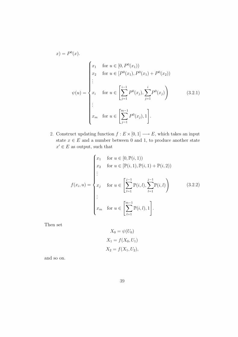
x) = P 0(x).

ψ(u) =

x1 for u ∈ [0, P 0(x1))

x2 for u ∈ [P 0(x1), P0(x1) + P 0(x2))

...

xi for u ∈[

i−1∑j=1

P 0(xj),i∑

j=1

P 0(xj)

)

...

xm for u ∈[

m−1∑j=1

P 0(xj), 1

].

(3.2.1)

2. Construct updating function f : E× [0, 1] −→ E, which takes an input

state x ∈ E and a number between 0 and 1, to produce another state

x′ ∈ E as output, such that

f(xi, u) =

x1 for u ∈ [0,P(i, 1))

x2 for u ∈ [P(i, 1),P(i, 1) + P(i, 2))...

xj for u ∈[

j−1∑

l=1

P(i, l),

j−1∑

l=1

P(i, l)

)

...

xm for u ∈[

m−1∑

l=1

P(i, l), 1

].

(3.2.2)

Then set

X0 = ψ(U0)

X1 = f(X0, U1)

X2 = f(X1, U2),

and so on.

39

Definition 3.2.1. The transition of a Markov chain X0, X1, . . . with tran-

sition matrix P can be described by a deterministic update function f by

Xt+1 = f(Xt, Ut+1) if

P(f(x, U) = y) = P(Xt+1 = y | Xt = x) = P (x, y) (3.2.3)

for all x, y ∈ E and for a uniform random number U .

Definition 3.2.2. A random map f : E → E is consistent with a Markov

chain with transition matrix P if P(f(x, U) = y) = P (x, y), for all x, y.

The transition rule is a random map which specifies for each state of E

the transition of the chain from time t to time t + 1.

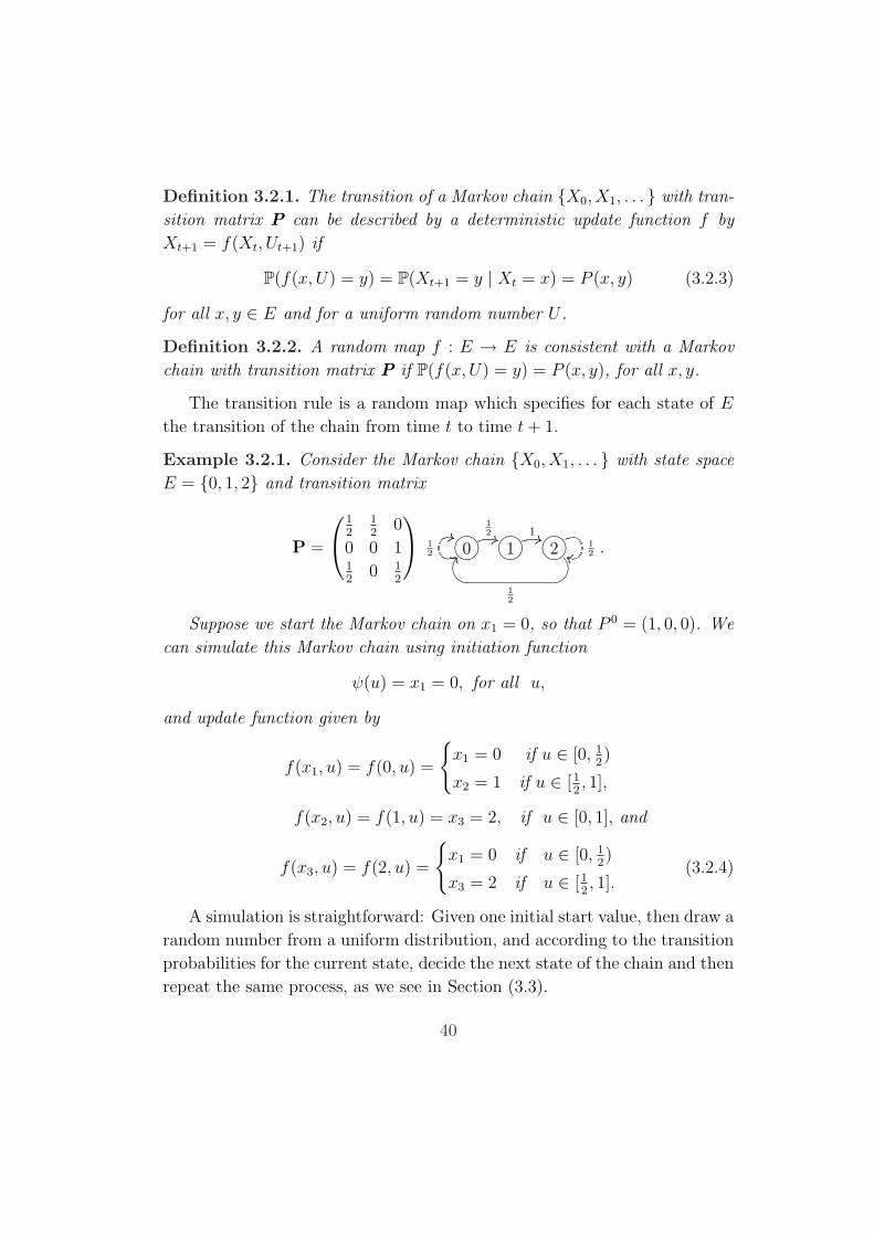
Example 3.2.1. Consider the Markov chain X0, X1, . . . with state space

E = 0, 1, 2 and transition matrix

P =

12

12

0

0 0 112

0 12

?>=<89:;01

2

))12 ** ?>=<89:;1

1 ** ?>=<89:;2 12iiBCD@GA

12

?? .

Suppose we start the Markov chain on x1 = 0, so that P 0 = (1, 0, 0). We

can simulate this Markov chain using initiation function

ψ(u) = x1 = 0, for all u,

and update function given by

f(x1, u) = f(0, u) =

x1 = 0 if u ∈ [0, 1

2)

x2 = 1 if u ∈ [12, 1],

f(x2, u) = f(1, u) = x3 = 2, if u ∈ [0, 1], and

f(x3, u) = f(2, u) =

x1 = 0 if u ∈ [0, 1

2)

x3 = 2 if u ∈ [12, 1].

(3.2.4)

A simulation is straightforward: Given one initial start value, then draw a

random number from a uniform distribution, and according to the transition

probabilities for the current state, decide the next state of the chain and then

repeat the same process, as we see in Section (3.3).

40

Definition 3.2.3. Two Markov chains X0, X1, . . . , X ′0, X

′1, . . . taking

their values in the same state space E are said to couple if there exists an

almost surely finite random time T such that

Xt = X′t for t ≥ T.

The random time T is called coupling time of the two chains, and obtain from

Theorem (3.1.1) that

‖ P(Xt = x)− P(X′t = x)‖ ≤ P(T > t),

since Xt 6= X ′t ⊂ T > t.

Definition 3.2.4. [13]Coalescence

A family of random processes X, Y, Z, . . . are said to coalesce if there is some

random time T (the coalescence time) at which they are all equal: X(T ) =

Y (T ) = Z(T ) = . . . Sometimes called grand coupling, since two processes

X, Y are said to couple if X(T ) = Y (T ) for some random time T .

Definition 3.2.5. We say that two chains have coalesced if they at one step

reach the same state. From that step and onward the two chains will follow

the same sample path, since they used the same updating function.

Definition 3.2.6. Convergence in Variation

Let X0, X1, . . . be a Markov chain with state space E. If for some proba-

bility distribution π on E, the distribution µ of Xt converges in variation to

π, that is

limt→∞

|P(Xt = x)− π(x)| = limt→∞

dTV (µ, π) = 0,

then X0, X1, . . . is said to converge in variation to π.

We are now ready to state the main result about convergence to station-

arity.

Theorem 3.2.1. [10] Markov chain convergence theorem.

Consider an irreducible aperiodic Markov chain X0, X1, . . . . If we denote

the chains distribution after the tth transition by P t, we have for any initial

distribution P 0 and a stationary distribution π

P t TV−−→ π (3.2.5)

41

In words: If we run the Markov chain for a long time, its distribution will

be very close to the stationary distribution π. This is often referred to as the

Markov chain approaching equilibrium as t −→∞.

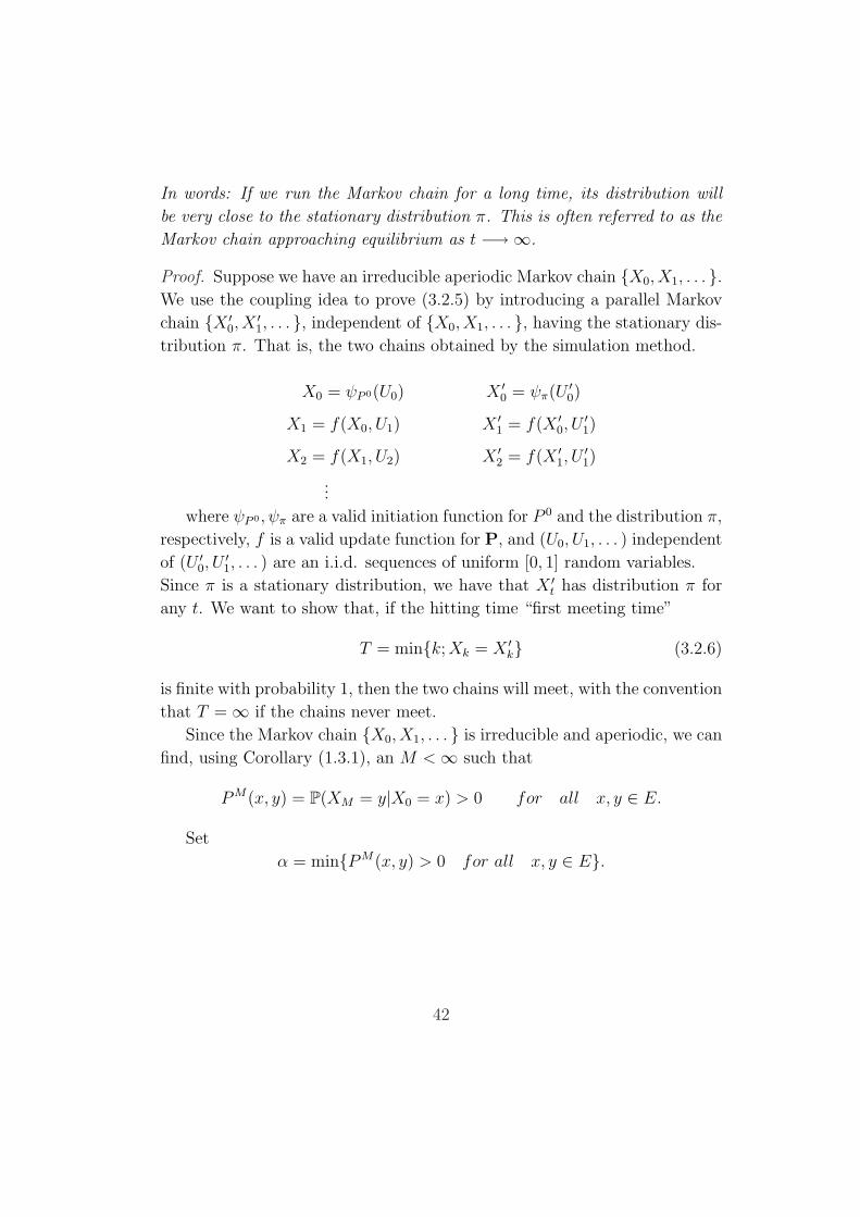
Proof. Suppose we have an irreducible aperiodic Markov chain X0, X1, . . . .We use the coupling idea to prove (3.2.5) by introducing a parallel Markov

chain X ′0, X

′1, . . . , independent of X0, X1, . . . , having the stationary dis-

tribution π. That is, the two chains obtained by the simulation method.

X0 = ψP 0(U0) X ′0 = ψπ(U ′

0)

X1 = f(X0, U1) X ′1 = f(X ′

0, U′1)

X2 = f(X1, U2) X ′2 = f(X ′

1, U′1)

...

where ψP 0 , ψπ are a valid initiation function for P 0 and the distribution π,

respectively, f is a valid update function for P, and (U0, U1, . . . ) independent

of (U ′0, U

′1, . . . ) are an i.i.d. sequences of uniform [0, 1] random variables.

Since π is a stationary distribution, we have that X ′t has distribution π for

any t. We want to show that, if the hitting time “first meeting time”

T = mink; Xk = X ′k (3.2.6)

is finite with probability 1, then the two chains will meet, with the convention

that T = ∞ if the chains never meet.

Since the Markov chain X0, X1, . . . is irreducible and aperiodic, we can

find, using Corollary (1.3.1), an M < ∞ such that

PM(x, y) = P(XM = y|X0 = x) > 0 for all x, y ∈ E.

Set

α = minPM(x, y) > 0 for all x, y ∈ E.

42

Then we get,

P(T ≤ M) ≥ P(XM = X ′M)

≥ P(XM = x1, X′M = x1)

= P(XM = x1)P(X′M = x1)

=

(m∑

i=1

P(X0 = xi, XM = x1)

)(m∑

i=1

P(X ′0 = xi, X

′M = x1)

)

=

(m∑

i=1

P(X0 = xi)P(XM = x1 | X0 = xi)

)(m∑

i=1

P(X ′0 = xi)P(X ′

M = x1|X ′0 = xi)

)

≥(

α

m∑i=1

P(X0 = xi)

)(α

m∑i=1

P(X ′0 = xi)

)= α2.

So that

P(T > M) ≤ 1− α2.

Similarly, given every thing that has happened up to time M , we have con-

ditional probability at least α2 of having X2M = X ′2M = x1. This implies

P(T > 2M) = P(T > M)P(T > 2M | T > M)

≤ (1− α2)P(T > 2M | T > M)

≤ (1− α2)P(X2M 6= X ′2M | T > M)

= (1− α2)(1− P(X2M = X ′2M | T > M))

≤ (1− α2)2.

By iterating this argument, we get for any l that

P(T > lM) ≤ (1− α2)l,

which tend to 0 as l →∞. Hence,

limt→∞

P(T > t) = 0. (3.2.7)

Therefore, the two chains will meet with probability 1.

Now, Define X ′′0 , X ′′

1 , . . . to make a coupling of X and X ′ at T which

is called the coupling time, by

X ′′t =

Xt if t < T

X ′t if t ≥ T,

(3.2.8)

43

where T as in (3.2.6). This implies that for all x ∈ E

| P(Xt = x)− π(x)| = | P(X ′′t = x)− P(X

′t = x)|

= | P(X ′′t = x, T ≤ t) + P(X ′′

t = x, T > t)

− P(X′t = x, T ≤ t)− P(X

′t = x, T > t)|

= | P(Xt = x, T > t)− P(X ′t = x, T > t)| due to (3.2.8)

≤ | P(Xt = x, T > t)− P(Xt = x,X ′t = x, T > t)|

= P(Xt = x, X ′t 6= x)

≤ P(Xt 6= X ′t)

≤ P(T > t),

which tend to 0 as t →∞. Hence,

limt→∞

|P t(x)− π(x)| = limt→∞

| P(Xt = x)− π(x)| = 0. (3.2.9)

This implies that

limt→∞

dTV (P t, π) = limt→∞

(1

2

m∑i=1

|P t(x)− π(x)|)

= 0 due to (3.2.9).

Hence, P t TV−−→ π.

Theorem 3.2.2. [10] Uniqueness of the stationary distribution.

Any irreducible and aperiodic Markov chain has exactly one stationary dis-

tribution.

Proof. By Theorem (1.5.1), an irreducible and aperiodic Markov chain has at

least one stationary distribution. So assume the chain X0, X1, . . . has more

than one stationary distribution, say π and π′. Then the chain distribution

after t transitions is P t = π′. On the other hand we have got

P t TV−−→ π.

Since P t = π′, meaning that lim dTV (π, π′) = 0 and this does not depend on

t at all, this implies dTV (π, π′) = 0. We conclude π = π′.

44

Remark 3.2.1. Even if a Markov chain has stationary distribution π, it may

still fail to converge to stationarity.

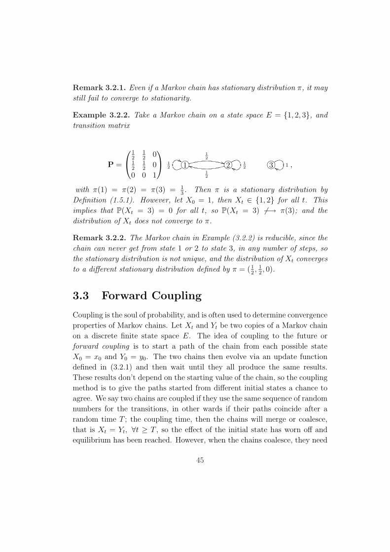
Example 3.2.2. Take a Markov chain on a state space E = 1, 2, 3, and

transition matrix

P =

12

12

012

12

0

0 0 1

/.-,()*+11

2

%%12

**/.-,()*+2 12ee

12

jj /.-,()*+3 1ee ,

with π(1) = π(2) = π(3) = 13. Then π is a stationary distribution by

Definition (1.5.1). However, let X0 = 1, then Xt ∈ 1, 2 for all t. This

implies that P(Xt = 3) = 0 for all t, so P(Xt = 3) 6−→ π(3); and the

distribution of Xt does not converge to π.

Remark 3.2.2. The Markov chain in Example (3.2.2) is reducible, since the

chain can never get from state 1 or 2 to state 3, in any number of steps, so

the stationary distribution is not unique, and the distribution of Xt converges

to a different stationary distribution defined by π = (12, 1

2, 0).

3.3 Forward Coupling

Coupling is the soul of probability, and is often used to determine convergence

properties of Markov chains. Let Xt and Yt be two copies of a Markov chain

on a discrete finite state space E. The idea of coupling to the future or

forward coupling is to start a path of the chain from each possible state

X0 = x0 and Y0 = y0. The two chains then evolve via an update function

defined in (3.2.1) and then wait until they all produce the same results.

These results don’t depend on the starting value of the chain, so the coupling

method is to give the paths started from different initial states a chance to

agree. We say two chains are coupled if they use the same sequence of random

numbers for the transitions, in other wards if their paths coincide after a

random time T ; the coupling time, then the chains will merge or coalesce,

that is Xt = Yt, ∀t ≥ T , so the effect of the initial state has worn off and

equilibrium has been reached. However, when the chains coalesce, they need

45

not have reached the stationary distribution, i.e., the state distribution of the

Markov chain at the coupling time is in general not equal to the stationary

distribution π, and this will not yield a correct algorithm, as the following

example show.

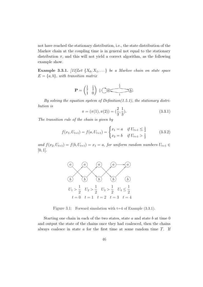
Example 3.3.1. [12]Let X0, X1, . . . be a Markov chain on state space

E = a, b, with transition matrix

P =

(12

12

1 0

)'&%$Ã!"#a1

2

%%12

**/.-,()*+b1

jj .

By solving the equation system of Definition(1.5.1), the stationary distri-

bution is

π = (π(1), π(2)) = (2

3,1

3). (3.3.1)

The transition rule of the chain is given by

f(x1, Ut+1) = f(a, Ut+1) =

x1 = a if Ut+1 ≤ 1

2

x2 = b if Ut+1 > 12

(3.3.2)

and f(x2, Ut+1) = f(b, Ut+1) = x1 = a, for uniform random numbers Ut+1 ∈[0, 1].

?>=<89:;a

ÂÂ???

????

???>=<89:;a

ÂÂ???

????

???>=<89:;a

ÂÂ???

????

???>=<89:;a // ?>=<89:;a

?>=<89:;b

??ÄÄÄÄÄÄÄÄÄ ?>=<89:;b

??ÄÄÄÄÄÄÄÄÄ ?>=<89:;b

??ÄÄÄÄÄÄÄÄÄ ?>=<89:;b

??ÄÄÄÄÄÄÄÄÄ ?>=<89:;b

U1 >1

2U2 >

1

2U3 >

1

2U4 ≤ 1

2

t = 0 t = 1 t = 2 t = 3 t = 4

Figure 3.1: Forward simulation with t=4 of Example (3.3.1).

Starting one chain in each of the two states, state a and state b at time 0

and output the state of the chains once they had coalesced, then the chains

always coalesce in state a for the first time at some random time T . If

46

X(1)T−1 6= X

(2)T−1, we necessarily obtain X

(1)T−1 = b or X

(2)T−1 = b and therefore

X(1)T = X

(2)T = a, because the chain moves deterministically to state a from

state b.

Figure 3.1 shows the forward simulation with stopping time T = 4 in state a

(XT = a), i.e., in distribution (1, 0). This does not agree with the stationary

distribution in (3.3.1), and hence XT 6∼ π, so the distribution at the time of

coalescence is not correct, that is the algorithm is incorrect.

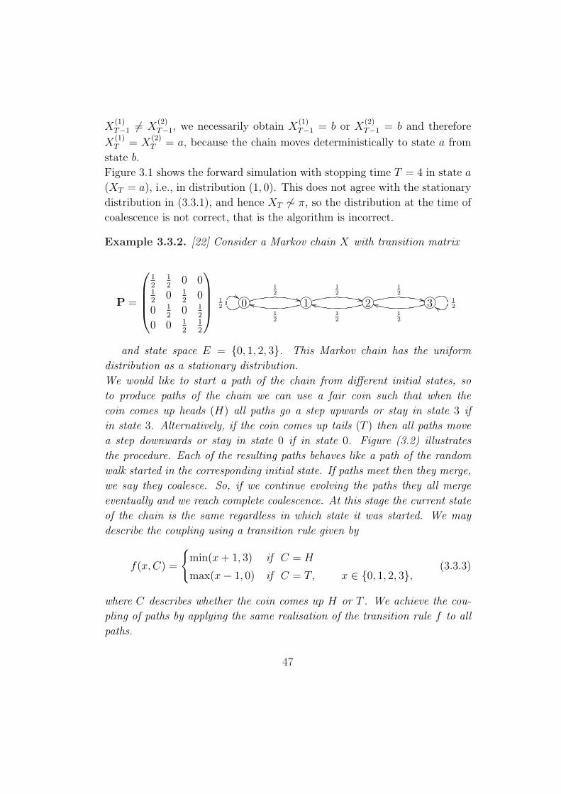
Example 3.3.2. [22] Consider a Markov chain X with transition matrix

P =

12

12

0 012

0 12

0

0 12

0 12

0 0 12

12

/.-,()*+012

%%12

**/.-,()*+112

jj

12

**/.-,()*+212

**

12

jj /.-,()*+312

jj 12ee

and state space E = 0, 1, 2, 3. This Markov chain has the uniform

distribution as a stationary distribution.

We would like to start a path of the chain from different initial states, so

to produce paths of the chain we can use a fair coin such that when the

coin comes up heads (H) all paths go a step upwards or stay in state 3 if

in state 3. Alternatively, if the coin comes up tails (T ) then all paths move

a step downwards or stay in state 0 if in state 0. Figure (3.2) illustrates

the procedure. Each of the resulting paths behaves like a path of the random

walk started in the corresponding initial state. If paths meet then they merge,

we say they coalesce. So, if we continue evolving the paths they all merge

eventually and we reach complete coalescence. At this stage the current state

of the chain is the same regardless in which state it was started. We may

describe the coupling using a transition rule given by

f(x,C) =

min(x + 1, 3) if C = H

max(x− 1, 0) if C = T, x ∈ 0, 1, 2, 3,(3.3.3)

where C describes whether the coin comes up H or T . We achieve the cou-

pling of paths by applying the same realisation of the transition rule f to all

paths.

47

?>=<89:;0

ÁÁ>>>

>>>>

>>?>=<89:;0 ?>=<89:;0 ?>=<89:;0 ?>=<89:;0

ÁÁ>>>

>>>>

>>?>=<89:;0 ?>=<89:;0 ?>=<89:;0 ?>=<89:;0

?>=<89:;1

ÁÁ>>>

>>>>

>>?>=<89:;1

ÁÁ>>>

>>>>

>>?>=<89:;1 ?>=<89:;1

@@¡¡¡¡¡¡¡¡¡ ?>=<89:;1

ÁÁ>>>

>>>>

>>?>=<89:;1

ÁÁ>>>

>>>>

>>?>=<89:;1 ?>=<89:;1 ?>=<89:;1

?>=<89:;2

ÁÁ>>>

>>>>

>>?>=<89:;2

ÁÁ>>>

>>>>

>>?>=<89:;2

@@¡¡¡¡¡¡¡¡¡ ?>=<89:;2

@@¡¡¡¡¡¡¡¡¡ ?>=<89:;2 ?>=<89:;2

ÁÁ>>>

>>>>

>>?>=<89:;2

ÁÁ>>>

>>>>

>>?>=<89:;2 ?>=<89:;2

?>=<89:;3 // ?>=<89:;3 // ?>=<89:;3

@@¡¡¡¡¡¡¡¡¡ ?>=<89:;3 ?>=<89:;3 ?>=<89:;3 ?>=<89:;3 // ?>=<89:;3

@@¡¡¡¡¡¡¡¡¡ ?>=<89:;3

H H T T H H H T

t = 0 t = 1 t = 2 t = 3 t = 4 t = 5 t = 6 t = 7 t = 8

Figure 3.2: Forward simulation for Example (3.3.2) with t=8.

Recall from Equation (3.2.3) that P(f(x, C) = y) = P (x, y), for all

x, y ∈ E = 0, 1, 2, 3 where P (x, y) are the transition probabilities of the

target chain X. Furthermore, at time t we update all states using the same

realisation of C. This is motivated by the fact that in this case

∀ x, y ∈ 0, 1, 2, 3, P(f(x,C) = f(y, C)) ≥3∑

z=0

P (x, z)P (y, z).

This means that at each step of our coupling the probability of two paths

merging when using the transition rule f is greater or equal than the prob-

ability of two paths merging in an independent coupling. An independent

coupling is achieved if we use an independent coin for each path.

At the time of complete coalescence, the chain is necessarily either in

state 0 or 3, which is not a sample of the stationary distribution (14, 1

4, 1

4, 1

4).

To solve this problem, there is a very effective modification enables us to

sample X in equilibrium. This modification is called backward coupling or

Coupling From The Past and is due to Propp and Wilson (1996).

48

Chapter 4

Perfect Simulation

4.1 Introduction

In 1906, Andry Markov produced the first result about a class of stochastic

processes. In such a process, the previous states are irrelevant for predicting

the subsequent states, given knowledge of the current state. This property

is now known as the Markov property. A generalization to countably in-

finite state spaces was given by Kolmogorov(1936). Markovian systems are

related to Brownian motion and the ergodic hypothesis, two topics in physics

which were important in the early years of the twentieth century. Markov

chain methods were then used as the building stone for generating sequences

of random numbers to accurately reflect very complicated desired proba-

bility distribution-a process called Markov Chain Monte Carlo (MCMC).

MCMC method is a class of algorithms for sampling from probability dis-

tributions, based on constructing a Markov chain that has the desired distri-

bution as its stationary distribution.

In the last ten years, the extensive use of MCMC methods to sample

from complicated multivariate probability distribution attracts much atten-

tion among statisticians ([6],[20],[23]).

In (1992) Asmussen et al.[1] gave the first algorithm for sampling from

the stationary distribution π of a Markov chain without knowledge of the

mixing time of the Markov chain “time that guarantees that the distribution

49

will not be much far from π whenever the chain starts”. They give a gen-

eral procedure, which given m and a Markov chain on m states, simulates

the Markov chain for a while, stops after a finite time, and then outputs a

random state distributed exactly according to π. Recent years have seen the

development of a new, exciting generation of MCMC: perfect or exact sim-

ulation algorithms. In contrast to conventional MCMC, perfect simulation

produces samples which are guaranteed to have exact equilibrium distribu-

tion, i.e., the feature of sampling after equilibrium has been reached is that

it produced samples which are guaranteed to have the target (desired) dis-

tribution and solve the problem of choosing an adequate burn in period.

Given a Markov chain which is irreducible and aperiodic that starts from

any probability distribution P , and run the chain for t steps, obtain the prob-

ability distribution P t which we want to be close to the desired distribution

π. As we mentioned in the introduction one of the long standing problems in

MCMC is that it is rarely possible to know when the Markov chain which

is used for simulation has reached equilibrium. This problem was solved in

(1995, 1996) by the introduction of Coupling From The Past which was in-

troduced by Propp and Wilson [18].

In this chapter, we discuss perfect simulation, beginning with ordinary

CFTP and moving on to the Dominated Coupling From The Past.

4.2 Coupling From The Past Algorithm

Coupling From The Past is an MCMC method devised by Propp and Wil-

son [18], also called backward coupling to produce a perfect sample from

the equilibrium distribution of a Markov chain through coupling multiple

Markov chains with the same equilibrium distribution but different initial

states. Consider a finite state space E with m states and an ergodic Markov

chain (irreducible and aperiodic) with stationary distribution π that can be

described by a deterministic update function f as in definition (3.2.1).

The idea of CFTP is to couple the Markov chain starting in all possible

states of E at some time −T < 0 in the past, and to run them until time

50

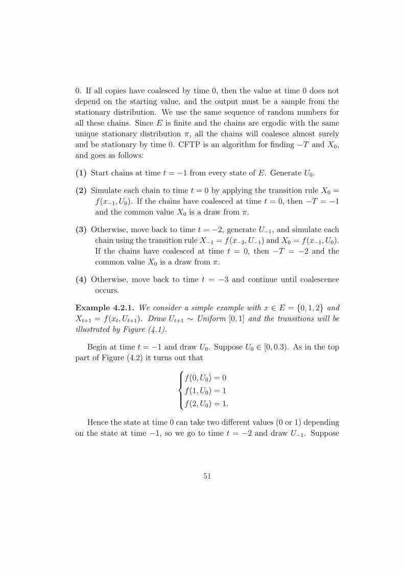
0. If all copies have coalesced by time 0, then the value at time 0 does not

depend on the starting value, and the output must be a sample from the

stationary distribution. We use the same sequence of random numbers for

all these chains. Since E is finite and the chains are ergodic with the same

unique stationary distribution π, all the chains will coalesce almost surely

and be stationary by time 0. CFTP is an algorithm for finding −T and X0,

and goes as follows:

(1) Start chains at time t = −1 from every state of E. Generate U0.

(2) Simulate each chain to time t = 0 by applying the transition rule X0 =

f(x−1, U0). If the chains have coalesced at time t = 0, then −T = −1

and the common value X0 is a draw from π.

(3) Otherwise, move back to time t = −2, generate U−1, and simulate each

chain using the transition rule X−1 = f(x−2, U−1) and X0 = f(x−1, U0).

If the chains have coalesced at time t = 0, then −T = −2 and the

common value X0 is a draw from π.

(4) Otherwise, move back to time t = −3 and continue until coalescence

occurs.

Example 4.2.1. We consider a simple example with x ∈ E = 0, 1, 2 and

Xt+1 = f(xt, Ut+1). Draw Ut+1 ∼ Uniform [0, 1] and the transitions will be

illustrated by Figure (4.1).

Begin at time t = −1 and draw U0. Suppose U0 ∈ [0, 0.3). As in the top

part of Figure (4.2) it turns out that

f(0, U0) = 0

f(1, U0) = 1

f(2, U0) = 1.

Hence the state at time 0 can take two different values (0 or 1) depending

on the state at time −1, so we go to time t = −2 and draw U−1. Suppose

51

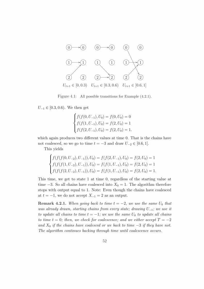
?>=<89:;0 // ?>=<89:;0 ?>=<89:;0 // ?>=<89:;0 ?>=<89:;0

ºº...

....

....

....

.?>=<89:;0

?>=<89:;1 // ?>=<89:;1 ?>=<89:;1

ÁÁ>>>

>>>>

>>?>=<89:;1 ?>=<89:;1 // ?>=<89:;1

?>=<89:;2

@@¡¡¡¡¡¡¡¡¡ ?>=<89:;2 ?>=<89:;2 // ?>=<89:;2 ?>=<89:;2

@@¡¡¡¡¡¡¡¡¡ ?>=<89:;2

Ut+1 ∈ [0, 0.3) Ut+1 ∈ [0.3, 0.6) Ut+1 ∈ [0.6, 1]

Figure 4.1: All possible transitions for Example (4.2.1).

U−1 ∈ [0.3, 0.6). We then get

f(f(0, U−1), U0) = f(0, U0) = 0

f(f(1, U−1), U0) = f(2, U0) = 1

f(f(2, U−1), U0) = f(2, U0) = 1.

which again produces two different values at time 0. That is the chains have

not coalesced, so we go to time t = −3 and draw U−2 ∈ [0.6, 1].

This yields

f(f(f(0, U−2), U−1)), U0) = f(f(2, U−1), U0) = f(2, U0) = 1

f(f(f(1, U−2), U−1)), U0) = f(f(1, U−1), U0) = f(2, U0) = 1

f(f(f(2, U−2), U−1)), U0) = f(f(1, U−1), U0) = f(2, U0) = 1.

This time, we get to state 1 at time 0, regardless of the starting value at

time −3. So all chains have coalesced into X0 = 1. The algorithm therefore

stops with output equal to 1. Note: Even though the chains have coalesced

at t = −1, we do not accept X−1 = 2 as an output.

Remark 4.2.1. When going back to time t = −2, we use the same U0 that

was already drawn, starting chains from every state; drawing U−1; we use it

to update all chains to time t = −1; we use the same U0 to update all chains

to time t = 0; then, we check for coalescence; and we either accept T = −2

and X0 if the chains have coalesced or we back to time −3 if they have not.

The algorithm continues backing through time until coalescence occurs.

52

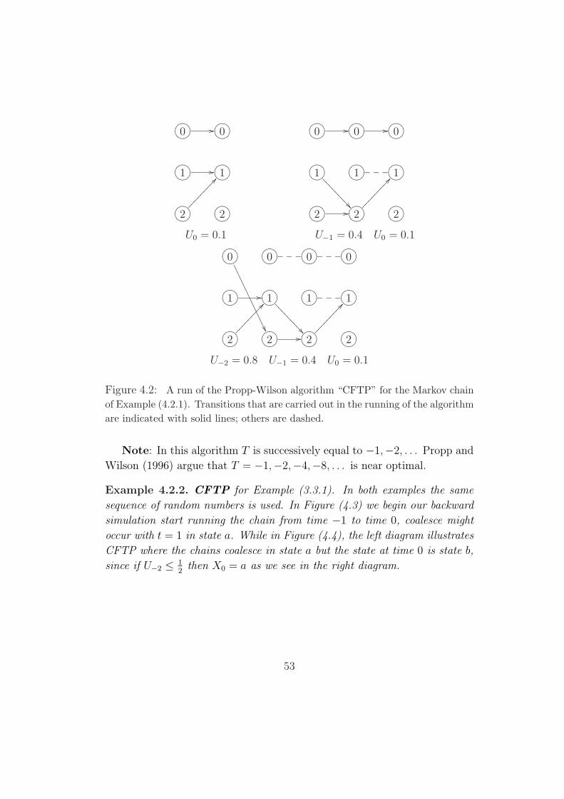
?>=<89:;0 // ?>=<89:;0 ?>=<89:;0 // ?>=<89:;0 // ?>=<89:;0

?>=<89:;1 // ?>=<89:;1 ?>=<89:;1

ÁÁ>>>

>>>>

>>?>=<89:;1 ___ ?>=<89:;1

?>=<89:;2

@@¡¡¡¡¡¡¡¡¡ ?>=<89:;2 ?>=<89:;2 // ?>=<89:;2

@@¡¡¡¡¡¡¡¡¡ ?>=<89:;2

U0 = 0.1 U−1 = 0.4 U0 = 0.1

?>=<89:;0

ºº...

....

....

....

.?>=<89:;0 ___ ?>=<89:;0 ___ ?>=<89:;0

?>=<89:;1 // ?>=<89:;1

ÁÁ>>>

>>>>

>>?>=<89:;1 ___ ?>=<89:;1

?>=<89:;2

@@¡¡¡¡¡¡¡¡¡ ?>=<89:;2 // ?>=<89:;2

@@¡¡¡¡¡¡¡¡¡ ?>=<89:;2

U−2 = 0.8 U−1 = 0.4 U0 = 0.1

Figure 4.2: A run of the Propp-Wilson algorithm “CFTP” for the Markov chainof Example (4.2.1). Transitions that are carried out in the running of the algorithmare indicated with solid lines; others are dashed.

Note: In this algorithm T is successively equal to −1,−2, . . . Propp and

Wilson (1996) argue that T = −1,−2,−4,−8, . . . is near optimal.

Example 4.2.2. CFTP for Example (3.3.1). In both examples the same

sequence of random numbers is used. In Figure (4.3) we begin our backward

simulation start running the chain from time −1 to time 0, coalesce might

occur with t = 1 in state a. While in Figure (4.4), the left diagram illustrates

CFTP where the chains coalesce in state a but the state at time 0 is state b,

since if U−2 ≤ 12

then X0 = a as we see in the right diagram.

53

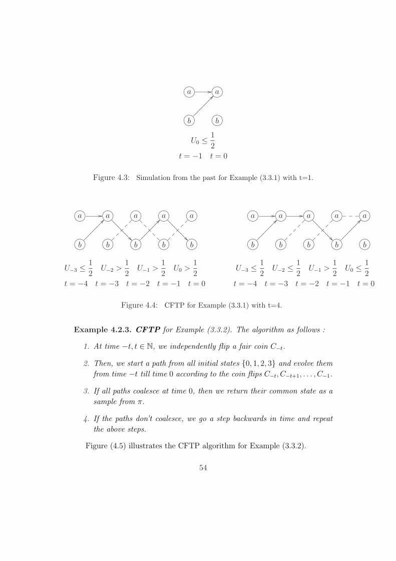
?>=<89:;a // ?>=<89:;a

?>=<89:;b

??ÄÄÄÄÄÄÄÄÄ ?>=<89:;b

U0 ≤ 1

2

t = −1 t = 0

Figure 4.3: Simulation from the past for Example (3.3.1) with t=1.

?>=<89:;a // ?>=<89:;a

ÂÂ???

????

???>=<89:;a

??

??

??>=<89:;a

ÂÂ???

????

???>=<89:;a ?>=<89:;a // ?>=<89:;a // ?>=<89:;a

ÂÂ???

????

???>=<89:;a ___ ?>=<89:;a

?>=<89:;b

??ÄÄÄÄÄÄÄÄÄ ?>=<89:;b

ÄÄ

ÄÄ

Ä ?>=<89:;b

??ÄÄÄÄÄÄÄÄÄ ?>=<89:;b

ÄÄ

ÄÄ

Ä ?>=<89:;b ?>=<89:;b

??ÄÄÄÄÄÄÄÄÄ ?>=<89:;b

ÄÄ

ÄÄ

Ä ?>=<89:;b

ÄÄ

ÄÄ

Ä ?>=<89:;b

??ÄÄÄÄÄÄÄÄÄ ?>=<89:;b

U−3 ≤ 1

2U−2 >

1

2U−1 >

1

2U0 >

1

2U−3 ≤ 1

2U−2 ≤ 1

2U−1 >

1

2U0 ≤ 1

2

t = −4 t = −3 t = −2 t = −1 t = 0 t = −4 t = −3 t = −2 t = −1 t = 0

Figure 4.4: CFTP for Example (3.3.1) with t=4.

Example 4.2.3. CFTP for Example (3.3.2). The algorithm as follows :

1. At time −t, t ∈ N, we independently flip a fair coin C−t.

2. Then, we start a path from all initial states 0, 1, 2, 3 and evolve them

from time −t till time 0 according to the coin flips C−t, C−t+1, . . . , C−1.

3. If all paths coalesce at time 0, then we return their common state as a

sample from π.

4. If the paths don’t coalesce, we go a step backwards in time and repeat

the above steps.

Figure (4.5) illustrates the CFTP algorithm for Example (3.3.2).

54

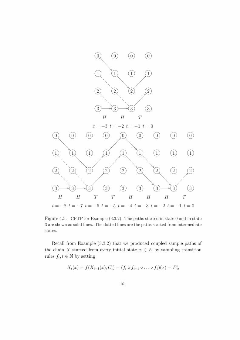
?>=<89:;0

ÁÁ>>>

>>>>

>>?>=<89:;0 ?>=<89:;0 ?>=<89:;0

?>=<89:;1

>>

>>

>?>=<89:;1

ÁÁ>>>

>>>>

>>?>=<89:;1 ?>=<89:;1

?>=<89:;2

>>

>>

>?>=<89:;2

>>

>>

>?>=<89:;2

@@¡¡¡¡¡¡¡¡¡ ?>=<89:;2

?>=<89:;3 // ?>=<89:;3 // ?>=<89:;3

@@¡¡¡¡¡¡¡¡¡ ?>=<89:;3

H H T

t = −3 t = −2 t = −1 t = 0

?>=<89:;0

ÁÁ>>>

>>>>

>>?>=<89:;0 ?>=<89:;0 ?>=<89:;0 ?>=<89:;0

ÁÁ>>>

>>>>

>>?>=<89:;0 ?>=<89:;0 ?>=<89:;0 ?>=<89:;0

?>=<89:;1

>>

>>

>?>=<89:;1

ÁÁ>>>

>>>>

>>?>=<89:;1 ?>=<89:;1

@@¡¡¡¡¡¡¡¡¡ ?>=<89:;1

ÁÁ>>>

>>>>

>>?>=<89:;1

ÁÁ>>>

>>>>

>>?>=<89:;1 ?>=<89:;1 ?>=<89:;1

?>=<89:;2

>>

>>

>?>=<89:;2

>>

>>

>?>=<89:;2

@@¡¡¡¡¡¡¡¡¡ ?>=<89:;2

@@¡¡¡¡¡¡¡¡¡ ?>=<89:;2 ?>=<89:;2

ÁÁ>>>

>>>>

>>?>=<89:;2

ÁÁ>>>

>>>>

>>?>=<89:;2 ?>=<89:;2

?>=<89:;3 // ?>=<89:;3 // ?>=<89:;3

@@¡¡¡¡¡¡¡¡¡ ?>=<89:;3 ?>=<89:;3 ?>=<89:;3 ?>=<89:;3 // ?>=<89:;3

@@¡¡¡¡¡¡¡¡¡ ?>=<89:;3

H H T T H H H T

t = −8 t = −7 t = −6 t = −5 t = −4 t = −3 t = −2 t = −1 t = 0

Figure 4.5: CFTP for Example (3.3.2). The paths started in state 0 and in state3 are shown as solid lines. The dotted lines are the paths started from intermediatestates.

Recall from Example (3.3.2) that we produced coupled sample paths of

the chain X started from every initial state x ∈ E by sampling transition

rules ft, t ∈ N by setting

Xt(x) = f(Xt−1(x), Ct) = (ft ft−1 . . . f1)(x) = F t0,

55

which becomes a constant function as t →∞ and f is defined as in (3.3.3).

In Figure (3.1) F t0(x) = a always, and in Figure (3.2) F t

0(x) = 2.

Propp and Wilson reverse the order of composition and have the equiva-

lent procedure

F 0−t = f−1 . . . f−t, t ∈ N.

Let F s−t = X−t

s (x) = f−s−1 . . . f−t(x), then X−ts (x),−t ≤ s ≤ 0

behaves like a path of X started at time −t in state x. Thus F 0−t(x) is

the state at time 0 of a path of X started at time −t in state x. The

transition rules f−t, t ∈ N describe transitions according to the transition

kernel P of X. As πP = π the transition rules preserve the equilibrium

distribution and so it follows that F 0−T (x) is also a sample from π, where

T = mint : F 0−t is a constant function.

In general: The idea of Coupling From The Past is simple.

Let Ut, t ∈ Z be independent, each chosen uniformly at random from [0, 1]

associated with time t. Consider the simulation of a Markov chain on E using

independent identically distributed transition map ft : E −→ E such that

ft(x) = f(x, Ut), where f is a deterministic function defined in (3.2.1). For

a chain (Xt), the function ft will define the evolution at time t. That is,

we construct a Markov chain X−t, . . . , X0 by constructing a set of update

functions fs(x, u), such that:

Xs = fs(Xs−1, Us), s = 0,−1, . . . ,−t

where Us is uniform at random variable on [0, 1].

For any realisation of the set of independent random variables U0, U−1, . . . , U−t

these update functions specify the transition from a state Xs−1 at time s to

a state Xs at time s + 1. If P (x, y) are the transition probabilities of the

Markov chain to move from x to y then the common distribution of the ft

should be such that P(ft(x, u) = y) = P (x, y).

Let t1 < t2 be integers, and

F t2t1 (x) = (ft2−1 ft2−2 . . . ft1)(x) = ft2−1(ft2−2(. . . ft1(x) . . . )).

Thus, F t2t1 defines the evolution from times t1 to t2, so F t

0 is the standard

forwards simulation for t steps starting at time 0, and F 0−t is the t−step

56

evolution of the Markov chain from time −t to time 0 (from the past). The

compositions F 0−t can be updated via the rule F 0

−t = F 0−t+1 f−t. More to the

point is the observation that if the map F 0−t ever becomes a constant map,

with F 0−t(x) = F 0

−t(y) for all x, y.

From (3.2.3) it follows that for every x, y ∈ E

P(F t2t1 (x, U) = y) = P t2−t1(x, y).

As F 0−t = X−t

0 = f−1 . . . f−t(x), then these update functions determine

a value of F 0−t = X−t

0 for all values of X−ts . If t is such that, for some x,

regardless of the value of X−ts , F 0

−t = X−t0 = x, then x is a draw from the

stationary distribution of the Markov chain. Therefore, if F 0−t maps the state

space to a single value, then for any t′ > t, F 0−t′ will also map the state space

to this same value. So with probability 1, all but finitely many of the random

variables F 0−1, F

0−2, . . . will take the same value.

Definition 4.2.1. Suppose that a Markov chain is defined via a random of

functions ft, t ∈ Z consistent with a transition matrix P as in Definition

(3.2.2). We refer to such a chain as a complete coupling chain. If F 0−t(x) =

F 0−t(y), we say that the two Markov chains X and Y have coupled. If F 0

−t

is a constant function, then we say that the chain has completely coupled at

time 0, and we denote the first time this occurs by T .

Theorem 4.2.1. [18] Suppose an ergodic Markov chain is constructed so

that there exists a time L < ∞ such that

P(FL0 (x, U) = y) = PL(x, y) > 0,

then,

(a) with probability 1 the CFTP algorithm returns a value, and

(b) this value is a realisation of a random variable distributed according to

the stationary distribution of the Markov chain.

Proof. (a) Since the chain is ergodic, there is an L such that for all states

x and y, there is a positive chance of going from x to y in L steps. let

F tt−L be the event that the chain started from all states in E at time t−l

57

have all coalesced by time t. Hence, F tt−L, ∀t has a positive chance

of being constant. Since each of the maps F−(k−1)L−kL , k ∈ 1, 2, . . .

has some positive probability of being constant, and since these map

are independent [because coalescence in (-kL, -(k-1)L)) only depends

on U−kL, U−kL+1, . . . , U−(k−1)L which are independent of all of the other

Us and does not depend on the initial states] and by assumption of the

theorem, it will happen with probability 1 that at least one of them is

constant. This implies that the algorithm terminates with probability

1.

(b) let T = mint : F 0−t is a constant function. Define

T ′ = mint : F 1−t is a constant.

Couple the Markov chain for F 0−t and F 1

−t, using the same ft′ at some

time t′ (hence T ′ ≤ T ). Let Z1−∞ = F 1

−T ′(X) be the constant value

of the function F 1−T ′ , and π0, π1 be the distribution of Z0

−∞ and Z1−∞,

respectively. Since Z0−∞, Z1

−∞ have the same probability distribution

(because they are the value of the constant function obtained by CFTP

up to some fixed time 0 or 1 respectively), we have π0 = π1. Since

Z1−∞ = f(Z0

−∞) is obtained from Z0−∞ by running the Markov chain

one step, the common distribution π0 = π1 is a fixed point of f , so it

must be the unique stationary distribution of the Markov chain.

A similar theorem can be found in [21],[24] with a slightly different proof.

Definition 4.2.2. A random variable T is called a stopping time with re-

spect to U−t , t = 0, 1, . . . if for any t, the event T ≤ t is determined by

U0, U−1, . . . , U−t.

The following theorem is an important tool in determining the mixing

time of a Markov chain.

Theorem 4.2.2. Suppose that we have a completely coupling chain, X0 has

some distribution over E and Y0 has a stationary distribution π. Then

dTV (F t0(X0), π) = ‖F t

0(X0)− π‖ ≤ P (Xt 6= Yt) = P(T > t).

58

Proof. By assumption, since Y0 has a stationary distribution π, then P(Yt ∈A) = π(A) for all A ⊂ E, so

‖F t0(X0)− π‖ = sup

A⊂E| P(Xt ∈ A)− π(A)|

= supA⊂E

| P(Xt ∈ A, T > t) + P(Xt ∈ A, T ≤ t)− P(Yt ∈ A)|

= supA⊂E

| P(Xt ∈ A, T > t) + P(Yt ∈ A, T ≤ t)

− (P(Yt ∈ A, T > t) + P(Yt ∈ A, T ≤ t))|= sup

A⊂E|P(Xt ∈ A, T > t)− P(Yt ∈ A, T > t)|

≤ supA⊂E

[supP(Xt ∈ A, T > t),P(Yt ∈ A, T > t)]

≤ supA⊂E

P(T > t)

= P(T > t).

Theorem 4.2.3. Assume that

1) the distribution of Ut , t ∈ Z is a stationary in time,

2) there exists a state x ∈ E so that for any event A ⊆ E, P(F t0(x) ∈ A) →

π(A) as t →∞, and

3) T ≥ 0 is an almost surely finite stopping time with respect to U−t , t =

0, 1, . . . such that F 0−t(x) = F 0

−T (x) whenever T ≤ t. Then F 0−T (x) ∼ π

Proof.

P(F 0−T (x) ∈ A) = P( lim

t→∞F 0−t(x) ∈ A)

= limt→∞

P(F 0−t(x) ∈ A) by monotone convergence theorem

= limt→∞

P(F t0(x) ∈ A) due to (1)

= π(A) due to (2).

59

4.3 Monotonicity and Anti-Monotonicity

As we saw, the method of simulating a Markov chain whose stationary dis-

tribution is the distribution we want to sample from is known in general as

MCMC. The traditional way to proceed is to run the Markov chain for a

long time (called the burn in time), so that by the end of this period the

Markov chain will be sufficiently close to stationarity that we may assume

that we are now sampling from the required distribution. The question is

“how long is long enough?”. One partial solution, (CFTP) was developed

by Propp and Wilson [18]. Other methods of sampling from the equilibrium

distribution of a Markov chain have since been developed, and the general

class of such algorithms is now commonly referred to as “Perfect Simulation”,

a name first coined by Kendall [12].

In Section (3.3), we showed how to couple paths of a Markov chain from

different initial states such that after a random time T , the paths have merged

into one. Although the state of any of these paths at this time doesn’t depend

on its starting value, it is still biased. This is because T is not a fixed time

but a random time. The solution to the biased sampling problem is to run

the chains from the past to the present, that is, we assume that at time −∞one chain is started in each of the states of E and run until 0. Also, we use

the same sequence of random numbers for all these chains. To see why this

gives a correct sampling scheme, Propp and Wilson assume that the state

space is finite with the following conditions:

Condition 1: There exist a partial ordering ¹ on the state space E :

that is, if Xt ¹ Yt, then

Xt+1 = f(Xt, Ut+1) ¹ f(Yt, Ut+1) = Yt+1, ∀ t.

Condition 2: ∃ xmin and xmax such that xmin ¹ x ¹ xmax for any state

x.

Monotonicity of P is guaranteed when one can couple transitions using a

monotone transition rule, and some Markov chains exhibits the property of

monotonicity, which depends on the existence of a partial ordering of the

state space E.

Definition 4.3.1. A partial order on E is a binary relation ¹ on E such

that, for all x, y, z ∈ E,

60

(i) x ¹ x,

(ii) x ¹ y and y ¹ x imply x = y,

(iii) x ¹ y and y ¹ z imply x ¹ z.

The set (E,¹) is said to be a partially ordered set (abbreviated: poset).

Definition 4.3.2. Suppose the functions ft, t ∈ Z determine a completely

coupling Markov chain. The Markov chain is said to be preserve the partial

order ¹ if for all x, y ∈ E and all times t, ft(x) ¹ ft(y) whenever x ¹ y.

Now by induction, if the Markov chain preserves the partial order, that

is X0 ¹ Y0, then F 0−t(X0) ¹ F 0

−t(Y0).

Definition 4.3.3. A monotone transition rule for a transition matrix P on a

partially ordered state space (E,¹) is a measurable function f : E×U −→ E,

together with a random number U taking values in an arbitrary probability

space U , such that:

(i) f(x, u) ¹ f(y, u) ∀ u ∈ U whenever x ¹ y,

(ii) P(f(x, u) = y) = P(Xt+1 = y | Xt = x) = P (x, y), for all x, y ∈ E,

(iii) Xt+1 = f(Xt, Ut+1) which present a Markov chain,

where the function f is the updating function, and the Ut+1 are i.i.d. sequence

distributed uniformly on [0, 1] defined in Section (3.2).

If all realisations of the random map are monotone functions, then we

call it a monotone transition rule, and when it exists, we can simultaneously

generate transitions from various states in such a way as to maintain relations

for each realisation. In other words, if we consider two paths generated by

the updating rule, using the same random sequence, and started in the states

x ¹ y, respectively, then with respect to ¹, the path started in x remains

beneath the path started in y.

Definition 4.3.4. When a monotone transition rule and xmin, xmax exist for

a given transition matrix P, we shall say that monotone case obtains.

61

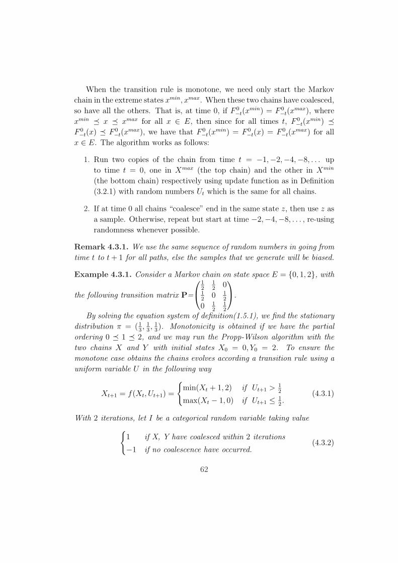
When the transition rule is monotone, we need only start the Markov

chain in the extreme states xmin, xmax. When these two chains have coalesced,

so have all the others. That is, at time 0, if F 0−t(x

min) = F 0−t(x

max), where

xmin ¹ x ¹ xmax for all x ∈ E, then since for all times t, F 0−t(x

min) ¹F 0−t(x) ¹ F 0

−t(xmax), we have that F 0

−t(xmin) = F 0

−t(x) = F 0−t(x

max) for all

x ∈ E. The algorithm works as follows:

1. Run two copies of the chain from time t = −1,−2,−4,−8, . . . up

to time t = 0, one in Xmax (the top chain) and the other in Xmin

(the bottom chain) respectively using update function as in Definition

(3.2.1) with random numbers Ut which is the same for all chains.

2. If at time 0 all chains “coalesce” end in the same state z, then use z as

a sample. Otherwise, repeat but start at time −2,−4,−8, . . . , re-using

randomness whenever possible.

Remark 4.3.1. We use the same sequence of random numbers in going from

time t to t + 1 for all paths, else the samples that we generate will be biased.

Example 4.3.1. Consider a Markov chain on state space E = 0, 1, 2, with

the following transition matrix P=

12

12

012

0 12

0 12

12

.

By solving the equation system of definition(1.5.1), we find the stationary

distribution π = (13, 1

3, 1

3). Monotonicity is obtained if we have the partial

ordering 0 ¹ 1 ¹ 2, and we may run the Propp-Wilson algorithm with the

two chains X and Y with initial states X0 = 0, Y0 = 2. To ensure the

monotone case obtains the chains evolves according a transition rule using a

uniform variable U in the following way

Xt+1 = f(Xt, Ut+1) =

min(Xt + 1, 2) if Ut+1 > 1

2

max(Xt − 1, 0) if Ut+1 ≤ 12.

(4.3.1)

With 2 iterations, let I be a categorical random variable taking value

1 if X, Y have coalesced within 2 iterations

−1 if no coalescence have occurred.(4.3.2)

62

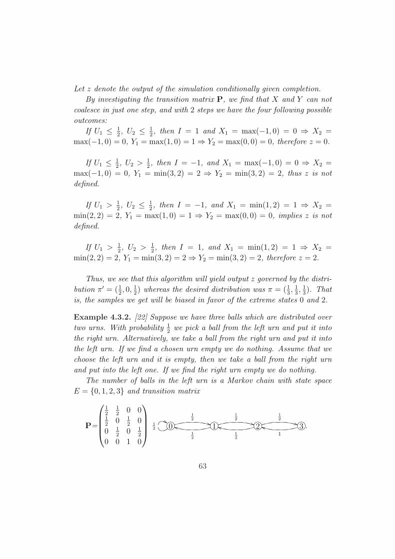
Let z denote the output of the simulation conditionally given completion.

By investigating the transition matrix P, we find that X and Y can not

coalesce in just one step, and with 2 steps we have the four following possible

outcomes:

If U1 ≤ 12, U2 ≤ 1

2, then I = 1 and X1 = max(−1, 0) = 0 ⇒ X2 =

max(−1, 0) = 0, Y1 = max(1, 0) = 1 ⇒ Y2 = max(0, 0) = 0, therefore z = 0.

If U1 ≤ 12, U2 > 1

2, then I = −1, and X1 = max(−1, 0) = 0 ⇒ X2 =

max(−1, 0) = 0, Y1 = min(3, 2) = 2 ⇒ Y2 = min(3, 2) = 2, thus z is not

defined.

If U1 > 12, U2 ≤ 1

2, then I = −1, and X1 = min(1, 2) = 1 ⇒ X2 =

min(2, 2) = 2, Y1 = max(1, 0) = 1 ⇒ Y2 = max(0, 0) = 0, implies z is not

defined.

If U1 > 12, U2 > 1

2, then I = 1, and X1 = min(1, 2) = 1 ⇒ X2 =

min(2, 2) = 2, Y1 = min(3, 2) = 2 ⇒ Y2 = min(3, 2) = 2, therefore z = 2.

Thus, we see that this algorithm will yield output z governed by the distri-

bution π′ = (12, 0, 1

2) whereas the desired distribution was π = (1

3, 1

3, 1

3). That

is, the samples we get will be biased in favor of the extreme states 0 and 2.

Example 4.3.2. [22] Suppose we have three balls which are distributed over

two urns. With probability 12

we pick a ball from the left urn and put it into

the right urn. Alternatively, we take a ball from the right urn and put it into

the left urn. If we find a chosen urn empty we do nothing. Assume that we

choose the left urn and it is empty, then we take a ball from the right urn

and put into the left one. If we find the right urn empty we do nothing.

The number of balls in the left urn is a Markov chain with state space

E = 0, 1, 2, 3 and transition matrix

P=

12

12

0 012

0 12

0

0 12

0 12

0 0 1 0

/.-,()*+012

%%12

**/.-,()*+112

jj

12

**/.-,()*+212

**

12

jj /.-,()*+31

jj .

63

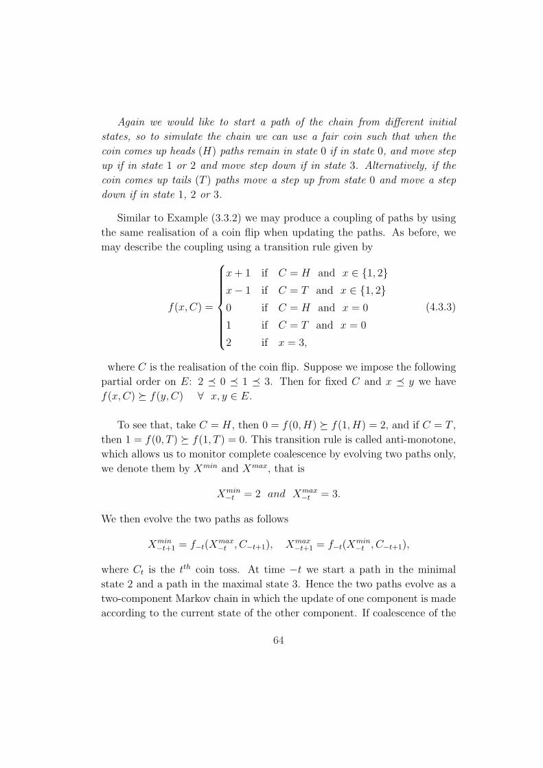
Again we would like to start a path of the chain from different initial

states, so to simulate the chain we can use a fair coin such that when the

coin comes up heads (H) paths remain in state 0 if in state 0, and move step

up if in state 1 or 2 and move step down if in state 3. Alternatively, if the

coin comes up tails (T ) paths move a step up from state 0 and move a step

down if in state 1, 2 or 3.

Similar to Example (3.3.2) we may produce a coupling of paths by using

the same realisation of a coin flip when updating the paths. As before, we

may describe the coupling using a transition rule given by

f(x,C) =

x + 1 if C = H and x ∈ 1, 2x− 1 if C = T and x ∈ 1, 20 if C = H and x = 0

1 if C = T and x = 0

2 if x = 3,

(4.3.3)

where C is the realisation of the coin flip. Suppose we impose the following

partial order on E: 2 ¹ 0 ¹ 1 ¹ 3. Then for fixed C and x ¹ y we have

f(x,C) º f(y, C) ∀ x, y ∈ E.

To see that, take C = H, then 0 = f(0, H) º f(1, H) = 2, and if C = T ,

then 1 = f(0, T ) º f(1, T ) = 0. This transition rule is called anti-monotone,

which allows us to monitor complete coalescence by evolving two paths only,

we denote them by Xmin and Xmax, that is

Xmin−t = 2 and Xmax

−t = 3.

We then evolve the two paths as follows

Xmin−t+1 = f−t(X

max−t , C−t+1), Xmax

−t+1 = f−t(Xmin−t , C−t+1),

where Ct is the tth coin toss. At time −t we start a path in the minimal

state 2 and a path in the maximal state 3. Hence the two paths evolve as a

two-component Markov chain in which the update of one component is made

according to the current state of the other component. If coalescence of the

64

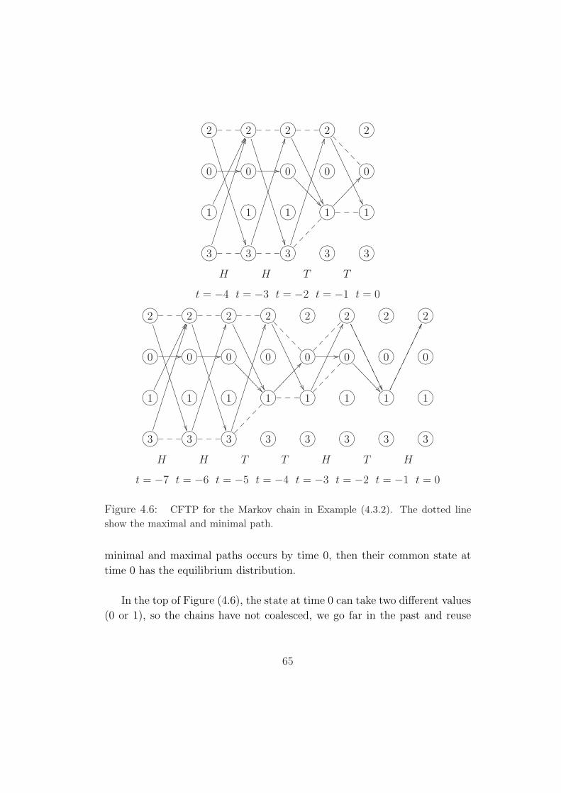
?>=<89:;2

··)))

))))

))))

))))

))))

))))

)___ ?>=<89:;2

··)))

))))

))))

))))

))))

))))

)___ ?>=<89:;2

ºº...

....

....

....

.___ ?>=<89:;2

ºº...

....

....

....

.

>>

>>

>?>=<89:;2

?>=<89:;0 // ?>=<89:;0 // ?>=<89:;0

ÁÁ>>>

>>>>

>>?>=<89:;0 ?>=<89:;0

?>=<89:;1

GG³³³³³³³³³³³³³³³³ ?>=<89:;1 ?>=<89:;1 ?>=<89:;1

@@¡¡¡¡¡¡¡¡¡___ ?>=<89:;1

?>=<89:;3

JJ¸¸¸¸¸¸¸¸¸¸¸¸¸¸¸¸¸¸¸¸¸¸¸

___ ?>=<89:;3

JJ¸¸¸¸¸¸¸¸¸¸¸¸¸¸¸¸¸¸¸¸¸¸¸

___ ?>=<89:;3

JJ¸¸¸¸¸¸¸¸¸¸¸¸¸¸¸¸¸¸¸¸¸¸¸

¡¡

¡¡

¡ ?>=<89:;3 ?>=<89:;3

H H T T

t = −4 t = −3 t = −2 t = −1 t = 0

?>=<89:;2

··)))

))))

))))

))))

))))

))))

)___ ?>=<89:;2

··)))

))))

))))

))))

))))

))))

)___ ?>=<89:;2

ºº...

....

....

....

.___ ?>=<89:;2

ºº...

....

....

....

.

>>

>>

>?>=<89:;2 ?>=<89:;2

ºº...

....

....

....

.

..

..

..

..

?>=<89:;2 ?>=<89:;2

?>=<89:;0 // ?>=<89:;0 // ?>=<89:;0

ÁÁ>>>

>>>>

>>?>=<89:;0 ?>=<89:;0 //

¡¡

¡¡

¡ ?>=<89:;0

ÁÁ>>>

>>>>

>>?>=<89:;0 ?>=<89:;0

?>=<89:;1

GG³³³³³³³³³³³³³³³³ ?>=<89:;1 ?>=<89:;1 ?>=<89:;1

@@¡¡¡¡¡¡¡¡¡___ ?>=<89:;1

GG³³³³³³³³³³³³³³³³

¡¡

¡¡

¡ ?>=<89:;1 ?>=<89:;1

GG³³³³³³³³³³³³³³³³

³³

³³

³³

³³ ?>=<89:;1

?>=<89:;3

JJ¸¸¸¸¸¸¸¸¸¸¸¸¸¸¸¸¸¸¸¸¸¸¸

___ ?>=<89:;3

JJ¸¸¸¸¸¸¸¸¸¸¸¸¸¸¸¸¸¸¸¸¸¸¸

___ ?>=<89:;3

JJ¸¸¸¸¸¸¸¸¸¸¸¸¸¸¸¸¸¸¸¸¸¸¸

¡¡

¡¡

¡ ?>=<89:;3 ?>=<89:;3 ?>=<89:;3 ?>=<89:;3 ?>=<89:;3

H H T T H T H

t = −7 t = −6 t = −5 t = −4 t = −3 t = −2 t = −1 t = 0

Figure 4.6: CFTP for the Markov chain in Example (4.3.2). The dotted lineshow the maximal and minimal path.

minimal and maximal paths occurs by time 0, then their common state at

time 0 has the equilibrium distribution.

In the top of Figure (4.6), the state at time 0 can take two different values

(0 or 1), so the chains have not coalesced, we go far in the past and reuse

65

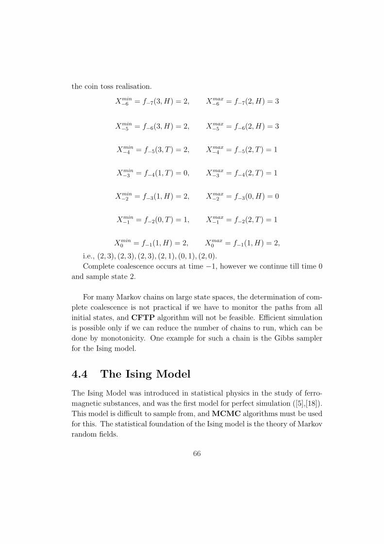
the coin toss realisation.

Xmin−6 = f−7(3, H) = 2, Xmax

−6 = f−7(2, H) = 3

Xmin−5 = f−6(3, H) = 2, Xmax

−5 = f−6(2, H) = 3

Xmin−4 = f−5(3, T ) = 2, Xmax

−4 = f−5(2, T ) = 1

Xmin−3 = f−4(1, T ) = 0, Xmax

−3 = f−4(2, T ) = 1

Xmin−2 = f−3(1, H) = 2, Xmax

−2 = f−3(0, H) = 0

Xmin−1 = f−2(0, T ) = 1, Xmax

−1 = f−2(2, T ) = 1

Xmin0 = f−1(1, H) = 2, Xmax

0 = f−1(1, H) = 2,

i.e., (2, 3), (2, 3), (2, 3), (2, 1), (0, 1), (2, 0).

Complete coalescence occurs at time −1, however we continue till time 0

and sample state 2.

For many Markov chains on large state spaces, the determination of com-

plete coalescence is not practical if we have to monitor the paths from all

initial states, and CFTP algorithm will not be feasible. Efficient simulation

is possible only if we can reduce the number of chains to run, which can be

done by monotonicity. One example for such a chain is the Gibbs sampler

for the Ising model.

4.4 The Ising Model

The Ising Model was introduced in statistical physics in the study of ferro-

magnetic substances, and was the first model for perfect simulation ([5],[18]).

This model is difficult to sample from, and MCMC algorithms must be used

for this. The statistical foundation of the Ising model is the theory of Markov

random fields.

66

Definition 4.4.1. Random Field

Let I be a vertex set, and let X = xi, i ∈ I be a random vector with

state space E defined on I. If we have P(X = x) = π(x) > 0 for all x ∈ E,

then we say we have a random field.

Definition 4.4.2. A collection δ = δ(i); i ∈ I of subsets of I is called a

neighbourhood system if

(i) i /∈ δ(i).

(ii) i ∈ δ(j) if and only if j ∈ δ(i).

The sites i ∈ δ(j) are called the neighbours of j, and we write i ∼ j if i

and j are neighbours.

Definition 4.4.3. Consider a finite set I of vertices, regarded as sites. A

configuration X = (xi; i ∈ I) assigns to each site i a spin xi, either +1

“upward” or −1 “downward”.

We denote (xi = σ | x−i) for the configuration whose spin at site i is σ

and whose spins at other sites agree with these for x.

Let π be a probability distribution on E and let x ∈ E with π(x) > 0.

If the site i is to be updated, the spin at this site is therefore set to

+1 with probability P(xi = +1 | x−i) =π(xi = +1, x−i)

π(xi = +1, x−i) + π(xi = −1, x−i)

−1 with the complementary probability P(xi = −1 | x−i).

(4.4.1)

These transition probabilities do not depend on xi.

We order the set of configuration by putting x ¹ y if and only if

xj ¹ yj for all j ∈ I.

Definition 4.4.4. [24] We say that π is attractive if the conditional proba-

bility of the event π(xi = 1 | x−i) is an increasing function of the values of

x−i (in the partial order).

67

Example 4.4.1. ([22],[24])Ising model:

The Ising model has energy function

E(x) = −J∑i∼j

xixj −∑

i

αixi,

where

xi= spin at site i of I,

i ∼ j =nearest neighbours in I,

J= the interaction strength between i and j, such that: when J > 0, the

state of lowest energy is when all spins are aligned. This is called a ferro-

magnetic, and J < 0 is an anti-ferromagnetic,

αi= external field measured at site i.

A certain spin configuration is chosen according to the probability distri-

bution π with

π(x) =1

zexp(−E(x)),

where z is the normalizing constant known as a “partition function”. Sam-

pling can be done effectively via Gibbs sampling with no need of calculating

the partition function z, to produce a Markov chain whose distribution con-

verges to the Ising model. Recall that the Gibbs sampling method updates one

site at a time, and that the conditional distribution is used as proposal.

Let x−i denotes the configuration x on I excluding the site i, then the

conditional probability of the Ising model having an upwards spin at site i

given the current spin configuration on all other sites is

P(xi = +1 | x−i) = π(xi = 1 | x−i)

=π(xi = +1, x−i)

π(xi = +1, x−i) + π(xi = −1, x−i). (4.4.2)

Let (xi = +1, x−i) be the configuration which we obtain by setting x = +1

and leaving the spins of all other sites in x unchanged, then from Equation

68

(4.4.2), we have

P(xi = +1 | x−i) = π(xi = 1 | x−i)

=

exp(J∑i∼j

xixj +∑

i

αixi)

exp(J∑i∼j

xixj +∑

i

αixi) + exp(−J∑i∼j

xixj −∑

i

αixi)

=

exp(J∑i∼j

xixj +∑

i

αixi) + exp(−J∑i∼j

xixj −∑

i

αixi)

exp(J∑i∼j

xixj +∑

i

αixi)

−1

= [1 + exp(−2J∑j∼i

xj − 2αi)]−1

= [1 + exp(−2(αi + J∑j∼i

xj))]−1,

(4.4.3)

which does not depend on the partition function z.

Remark 4.4.1. Since Equation (4.4.3) is increasing in x−i, the Gibbs sam-

pler is monotone for the Ising model with an external field.

Proof. We can couple paths of the Gibbs Sampler started from different

initial states by reusing the sampled random variates Ut+1 and Nt+1, such

that Ut+1 is uniformly distributed on [0, 1] and Nt+1 is drawn uniformly on

(1, . . . , n). At time t we update the same site Nt+1 in each path using the

same realisation of Ut+1 for all paths.

We may defined the Gibbs sampler through the update function f given

by

f(x, U,N) =

(xN = +1, x−N) if U ≤ P(xN = +1 | x−N)

(xN = −1, x−N) otherwise.(4.4.4)

To show that f is monotone, we need to show that f(x, U,N) ¹ f(y, U,N)

for fixed U,N, when x ¹ y.

Now if the system is attractive then, π(xN = 1 | x−N) ¹ π(yN = 1 | y−N)

for x ¹ y, hence P(xN = +1 | x−N) ≤ P(yN = +1 | y−N). Thus, for fixed

U,N, we have

69

1. Whenever f assigns an upwards spin to xN then, it also assigns an

upwards spin to yN , as U ≤ P(xN = +1 | x−N) ≤ P(yN = +1 | y−N).

2. Analogously, whenever f assigns a downward spin to yN then, it assigns

a downward spin to xN .

Thus, if x ¹ y then, the updated configurations maintain their partial order-

ing, that is, f(x, U,N) ¹ f(y, U,N) for fixed U,N. Therefore our transition

rule f is monotone with respect to ¹ .

The basic idea of the Propp-Wilson method is not to run the Markov chain

forward in time, but rather to run the Markov chain from time −t in the past

up to time t = 0. CFTP can be used in the Ising model by running two

coupled realisations X and Y of the Markov chains (two spin configurations),

starting in the maximal and minimal states at some time −t in the past, with

all spin up or all spin down, using the updating function f defined in (4.4.4),

such that Xt+1 = f(Xt, Ut+1, Nt+1) and Yt+1 = f(Yt, Ut+1, Nt+1). [The same

random numbers are used for each spin configurations]. If X0 = Y0, then

this value is our sample. That is, if the two chains have coupled at time 0,

the state at time 0 is an exact sample from the Markov chain’s stationary

distribution.

Since f is monotone, we have that F t2t1 (E) is constant ⇐⇒ F t2

t1 (xmin) =

F t2t1 (xmax), where xmin, xmax ∈ E. The coupling time of f is the smallest T

such that F T0 (xmin) = F T

0 (xmax). The coupling from the past time of f is

the smallest M such that F 0−M(xmin) = F 0

−M(xmax). We have that

P(T > t) = P(F t0(x

min) 6= F t0(x

max)) = P(F 0−t(x

min) 6= F 0−t(x

max)) = P(M > t).

Hence M has the same distribution as T .

4.5 Dominated Coupling From The Past

It follows from the very existence of CFTP constructions that all the chains

discussed so far have been uniformly ergodic.

70

Definition 4.5.1. A Markov chain having stationary distribution π is uni-

formly ergodic if

dTV (P t(x), π) = ‖P t(x)− π‖ ≤ Mρt, t = 1, 2, . . .

for some ρ < 1 and M < ∞.

If the Markov chain is not uniformly ergodic, what should we use?

Suppose T ≥ 0 is the smallest random time such that coupled paths of the

target chain started in all initial states at time −T have coalesced by time 0.

As pointed in [6], uniform ergodicity is a sufficient and necessary property for

applying the Propp and Wilson algorithm, the failure of uniform ergodicity

implies that coalescence of the Markov chain can not happen in finite time,

so the original CFTP algorithm of finite state space E of [18] needs modi-

fication. This modification is an extension of the original CFTP algorithm,

called Dominated coupling from the past (DCFTP) or horizontal CFTP,

which is an example of perfect simulation for sampling from the equilibrium

distribution of a Markov chain.

In [6], vertical CFTP is a coupling of realisations started at a fixed time for

all possible initial states, while horizontal CFTP is a coupling of realisations

started at the minimal state at all sufficiently early initial times.

The idea of DCFTP is as follows: generate target chains coupled to

dominating process for which equilibrium is known. We consider a discrete

time monotic chain defined on [0,∞).

Definition 4.5.2. [13]DCFTP

Consider X, an ergodic Markov chain on [0,∞). Suppose it can be coupled

as follows: for each x ≥ 0,−t < 0 we can construct X−t(x) to be X begun at

x at time −t, such that if s ≥ −t, s ≥ −u, then

X−ts (x) ≤ X−u

s (y) implies X−ts+1(x) ≤ X−u

s+1(y).

Furthermore, suppose we can build a dominating process Y on [0,∞), which

is stationary, defined for all time, and coupled to the X−t(x) by

X−ts (x) ≤ Ys implies X−t

s+1(x) ≤ Ys+1,

71

whenever s ≥ −t. Then the following algorithm delivers a perfect sample

from the equilibrium distribution of X, so long as it terminates almost surely:

(1) Draw Y0 from its equilibrium distribution;

(2) Simulate Y backwards in time to time −T ;

(3) Set y = Y−T , and simulate the upper process X−T (y) and the lower

process X−T (0) forwards in time to time 0 (The upper and lower must

be coupled to each other, to Y , and at later stages of the algorithm

they must be coupled to other simulations of X at the same process

time);

(4) If X−T0 (y) = X−T

0 (0), then return their common value as a perfect

draw from the equilibrium distribution of X. Otherwise, extend the

previous simulation of Y back to time −2T , update −T to −2T , and

repeat from step (3).

Theorem 4.5.1. [13],[22] If coalescence is almost sure then dominated CFTP

samples from equilibrium.

Proof. Suppose the target process X is monotone, and that it and the dom-

inating process Y are nonnegative.

Let Xupper,−t, X lower,−t = X−t be versions of the target chain started at

time −t at Y (−t), 0 respectively. Let

T = inft ≥ 0 : Xupper,−t(0) = X lower,−t(0),so, −T (the coalescence time) is the latest time such that Xupper,−T (0) =

X lower,−T (0) = X−T (0). So,

X−t0 = X−T

0 whenever− t ≤ −T ;

L(X−t0 ) = L(X0

t ), where X−ts = F s

−t(0) for −t ≤ s.

If X converges to an equilibrium π in total variation dTV , then

dTV (L(X−T0 ), π) = lim

tdTV (L(X−t

0 ), π) = limt

dTV (L(X0t ), π) = 0.

This proves the theorem.

72

Conclusion

Random sampling has found numerous applications in computer science, sta-

tistics, and physics. The most widely applicable method of random sampling

is to use a Markov chain whose stationary distribution is the probability

distribution π from which we wish to sample. After the Markov chain has

been run for long enough, its state is distributed exactly according to π. The

principal problem with this approach is that it is often difficult to determine

how long to run the Markov chain. This thesis provides the motivation for

perfect simulation. It begins with the concept of a Markov chain on finite

state space, and attempts to explain and summaries MCMC algorithms.

Then gives a review of the basic ideas in the new methods of perfect simula-

tion, the concepts of Coupling From The Past, which is a class of algorithms

for generating perfectly random samples from a Markov chain in the discrete

case, produces samples which are guaranteed to have the exact equilibrium

distribution. We have seen that CFTP of uniformly ergodic Markov chain

is based on couplings of paths of the target Markov chain started in different

initial states such that after an almost surely finite time the paths coincide

(they merge into one or coalesce), and does not depend on its starting value.

Monotonicity and anti-monotonicity with respect to a partial order of the

chosen coupling help in checking for complete coalescence by reducing the

number of paths to run into lower and upper path, such that if they coa-

lesce at time 0, their common state is an exact sample from the stationary

distribution. If the Markov chain is not uniformly ergodic, we have to use

DCFTP.

73

Bibliography

[1] Asmussen, S., Glynn, P.W. and Thorisson, H. Stationary detection in the

initial transient problem, ACM Transactions on Modeling and Computer

Simulation, 2(2)( 1992), 130-157.

[2] Casella, G. and George, E. I. Explaining the Gibbs sampler , Am. Stat.

46(1992), 167-174.

[3] Durrett, R. Probability: Theory and Examples, Wadsworth Publishing

Company, Second Edition, 1996.

[4] Evans, Michael J. and Rosenthal, J. S. probability and statistics, The

science of Uncertainty, W. H. Freeman and Company, NewYork, 2003.

[5] Fill, J.A. An interruptible algorithm for perfect sampling via Markov

chains, Annals of Applied Probability, 8( 1998), 131-162.

[6] Foss, S.G. and Tweede, R.L. Perfect simulation and backward coupling,

Stochastic models 14( 1998), 187-203.

[7] Gelfand, A.E. and Smith, A.F.M. Sampling based approaches to calculat-

ing marginal densities, Journal of the American Statistical Association,

85(1990), 398-409.

[8] Geman, S. and Geman, D. Stochastic Relaxation, Gibbs Distributions,

and the Bayesian Restoration of Images, I.E.E.E. Trans. On Patten

Analysis Machine Intelligence, 6(1984), 721-741.

74

[9] Gilks, W.R., Richardson, S. and Spiegelhater, D.J. Markov Chain Monte

Carlo In Practice, Chapman and Hall, London, 1996.

[10] Haggstrom, O. Finite Markov Chains and Algorithmic Applications,

Cambridge University Press, 2000.

[11] Hastings, W.K. Monte Carlo sampling using Markov chains and their

Applications Biometrika, 57(1970), 97-109.

[12] Kendall, W.S. and Thonnes, E. Perfect Simulation in Stochastic Geom-

etry, 1998.

[13] Kendall, W.S., Liang, F. and Wang, J-S. Markov Chain Monte Carlo

Innovations and Applications, World Scientific Publishing Co. Pte. Ltd.,

2005.

[14] Lindvall, T. Lectures on the Coupling Method, Dover Publications Inc.,

Mineola, NY, 2002.

[15] Metropolis, N., Rosenbluth, A.W., Rosenbluth, M.N., Teller, A.H. and

Teller, E. Equations Of State Calculations by Fast Computing Machine,

Journel of chemical physics, Vd., 21( 1953), 1087-1092.

[16] Mφller, J. A Note On Perfect Simulation of Conditionally Specified Mod-

els, 1997.

[17] Murdoch, D.J. and Rosenthal, J.S. An extension of Fill’s exact sampling

algorithm to non-monotone chains, 1998.

[18] Propp, J.G. and Wilson, D.B. Exact Sampling With Coupled Markov

Chains and applications to statistical mechanics, Random Structures

Algorithms, 9( 1996), 223-252.

[19] Shiryayev, A.N. Probability, Springer-Verlag , NewYork, 1984.

[20] Smith, A.F.M. and Robert, G.G. Bayesian computation via the Gibbs

sampler and related Markov chain Monte Carlo methods, Journel of the

Royal Statistical Society, Series B(1993), 553-23.

75

[21] Thonnes, E. A primer on Perfect Sampling, International Statistical

Review, 69(1)( 2000), 27-48.

[22] Thonnes, E. A primer on Perfect Simulation, Technical report, Depart-

ment of Mathematical Statistics, Chalmers University of Technology,

1999.

[23] Tierney, L. Markov Chains for exploring posterior distributions, (with

discussion). Annals of statistics, 22( 1994), 1701-1762.

[24] Xeni, k. Dimakos. A Guide To Exact Simulation, Statistical Physics and

Spatial Statistic, ed. Klaus R. Mecke and D. stoyan, Springer Lecture

Notes in physics, 554(2001), 349-378.

76