compound poisson integer-valued garch processes po… · na literatura vários modelos para séries...
TRANSCRIPT

Filipa Alexandra Cardoso da Silva
COMPOUND POISSON INTEGER-VALUED
GARCH PROCESSES
Tese de Doutoramento do Programa Inter-Universitário de Doutoramento
em Matemática, orientada pela Professora Doutora Maria de Nazaré
Mendes Lopes e pela Professora Doutora Maria Esmeralda Gonçalves e
apresentada ao Departamento de Matemática da Faculdade de Ciências e
Tecnologia da Universidade de Coimbra.
Fevereiro 2016


Compound Poisson integer-valuedGARCH processes
Filipa Alexandra Cardoso da Silva
UC|UP Joint PhD Program in Mathematics
Programa Inter-Universitário de Doutoramento em Matemática
PhD Thesis | Tese de Doutoramento
February 2016


Acknowledgements
Firstly, I would like to express my sincere gratitude to my advisors Prof. Dr. Nazaré and Prof. Dr.Esmeralda for the continuous support on my PhD, for their patience, generosity, dedication, motivationand immense knowledge. Their excellent guidance helped me in all the time of research and writingof this thesis. I could not have imagined having better advisors for my PhD study. It was an honor towork with them and to have been their student in several subjects during my training.
Besides my advisors, I would like to thank the rest of my professors that along this work gave mesome support and caring, in particular, the Prof. Dr. Adérito who always helped me with my Matlabquestions and the Prof. Dr. José Augusto for his encouraging words and advices. My sincere thanksalso goes to Prof. Dr. Christian H. Weiß and Prof. Dr. René Ferland, for their availability to visitDMUC, for their valuable comments and for the great and stimulating seminars that they provided us.
A special thanks to the Fundação para a Ciência e a Tecnologia and to the Centro de Matemáticada Universidade de Coimbra for their financial support which was essential for the development anddissemination of my work. Without them it would not be possible to conduct this research.
To the DMUP that welcomed me for one year, to the DMUC that once again proved to be a greatinstitution providing me an excellent atmosphere for doing research and for the Steering Committeeof the PhD Program in Mathematics, for them also I reserve my gratitude.
I would like to thank my old friends and the new ones that this experience gave me. As Cicerosaid: "Life is nothing without friendship". I would also like to thank Joana Leite, the better roommateand traveling companion of international conferences I could have had. For her willingness to helpme, for her support, advices, and for the great experiences we shared. My sincere thanks also goes tomy friend Fernando Marçal who kindly ceded me his painting for the front cover of this thesis.
Last but not the least, I would like to thank my family: my parents, my sisters and my godparents.They were always supporting me and encouraging me with their best wishes, they never let medemotivate. Thank you Júlia for all the fun we have had in the last four years and for endure my longspeeches about football. Thank you mother for letting me sleep late. Thank you parents, Elsa andgodfather for being my drivers when I needed.


Abstract
Count time series modeling has drawn much attention and considerable development in the recentdecades since many of the observed stochastic systems in various contexts and scientific fields aredriven by such kind of data. The first modelings, with linear character and essentially inspired by theclassic ARMA models, are proved to be insufficient to give an adequate answer for some empiricalcharacteristics, also observed in this type of data, such as the conditional heteroscedasticity. In orderto capture such kind of characteristics several models for nonnegative integer-valued time series arisein literature inspired by the classic GARCH model of Bollerslev [10], among which is highlightedthe integer-valued GARCH model with conditional Poisson distribution (briefly INGARCH model),proposed in 2006 by Ferland, Latour and Oraichi [25].
The aim of this thesis is to introduce and analyze a new class of integer-valued models havingan analogous evolution as considered in [25] for the conditional mean, but with an associatedcomprehensive family of conditional distributions, namely the family of infinitely divisible discretelaws with support in N0, inflated (or not) in zero. So, we consider a family of conditional distributionsthat in its more general form can be interpreted as a mixture of a Dirac law at zero with any discreteinfinitely divisible law, whose specification is made by means of the corresponding characteristicfunction. Taking into account the equivalence, in the set of the discrete laws with support N0, betweeninfinitely divisible and compound Poisson distributions, this new model is designated as zero-inflatedcompound Poisson integer-valued GARCH model (briefly ZICP-INGARCH model).
We point out that the model is not limited to a specific conditional distribution; moreover, thismodel has as main advantage to unify and enlarge substantially the family of integer-valued stochasticprocesses. It is stressed that it is possible to present new models with conditional distributions withinterest in practical applications as, in particular, the zero-inflated geometric Poisson INGARCH andthe zero-inflated Neyman type-A INGARCH models, and also recover recent contributions such as the(zero-inflated) negative binomial INGARCH [81, 84], (zero-inflated) INGARCH [25, 84] and (zero-inflated) generalized Poisson INGARCH [52, 82] models. In addition to having the ability to describedifferent distributional behaviors and consequently, different kinds of conditional heteroscedasticity,the ZICP-INGARCH model is able to incorporate simultaneously other stylized facts that have beenrecorded in real count data, in particular overdispersion and high occurrence of zeros.
The probabilistic analysis of these models, concerning in particular the development of necessaryand sufficient conditions of different kinds of stationarity (first-order, weak and strict) as well as theproperty of ergodicity and also the existence of higher order moments, is the main goal of this study.It is still derived estimates for the parameters of the model using a two-step approach which is basedon the conditional least squares and moments methods.


Resumo
A modelação de séries temporais de contagem conheceu nas últimas décadas grande impulso edesenvolvimento, devido sobretudo ao fato de muitos dos sistemas estocásticos observados, nos maisdiversos contextos e áreas científicas, terem como resposta tal tipo de dados. As primeiras modelações,de caráter linear e essencialmente inspiradas nos clássicos modelos ARMA, revelaram-se insuficientespara dar resposta a algumas características empíricas, também observadas neste tipo de dados, comoa heteroscedasticidade condicional. De modo a ter em conta tal tipo de características, surgiramna literatura vários modelos para séries temporais de valores inteiros não negativos inspirados nosGARCH clássicos de Bollerslev [10], entre os quais se destacam os modelos GARCH de valoresinteiros com distribuição condicional de Poisson (designados modelos INGARCH), propostos em2006 por Ferland, Latour e Oraichi [25].
O objetivo fundamental deste trabalho é introduzir e analisar uma nova classe de modelos devalores inteiros com evolução para a média condicional análoga à considerada em [25] mas emque se considera associada uma família abrangente de leis condicionais, nomeadamente a das leisinfinitamente divisíveis discretas com suporte em N0, inflacionadas (ou não) em zero. Consideramosentão uma família de leis condicionais que, na sua forma mais geral, podem ser interpretadas comomisturas de uma lei de Dirac com uma qualquer lei discreta infinitamente divisível, sendo a suaespecificação feita através da função característica. Em consequência da equivalência, no conjuntodas leis discretas com suporte N0, entre leis infinitamente divisíveis e leis de Poisson compostas, estenovo modelo denomina-se modelo GARCH de valor inteiro Poisson Composto inflacionado em zero(abreviadamente ZICP-INGARCH).
Para além de não se limitar a considerar como lei condicional uma lei específica, este modelotem como principal vantagem unificar e alargar significativamente a família de processos estocásticosde valores inteiros. Destaca-se que é possível evidenciar novos modelos com leis condicionais cominteresse nas aplicações práticas como, em particular, os modelos INGARCH Poisson geométrico eINGARCH Neyman tipo-A eventualmente inflacionados em zero, e também reencontrar contribuiçõesrecentes como os modelos INGARCH binomial negativo [81, 84], INGARCH Poisson [25, 84] eINGARCH Poisson generalizado [52, 82] eventualmente inflacionados em zero. Para além de ter acapacidade de descrever diferentes comportamentos distribucionais e, consequentemente, diferentestipos de heteroscedasticidade condicional, o modelo ZICP-INGARCH consegue incorporar outrosfactos estilizados muito associados a séries de contagem, nomeadamente a sobredispersão e a elevadaocorrência de zeros. A análise probabilista destes modelos, no que diz respeito em particular aodesenvolvimento de condições necessárias e suficientes de estacionaridade (de primeira ordem, forte efraca) e ergodicidade e também de existência de momentos de ordem elevada, é o objeto principaldeste estudo. São ainda determinados estimadores para os parâmetros do modelo seguindo umametodologia em duas etapas que envolve o método dos mínimos quadrados e o dos momentos.

Table of contents
List of figures xi
List of tables xiii
1 Introduction 11.1 Count time series . . . . . . . . . . . . . . . . . . . . . . . . . . . . . . . . . . . . 11.2 A review in count data literature . . . . . . . . . . . . . . . . . . . . . . . . . . . . 31.3 Overview of the Thesis . . . . . . . . . . . . . . . . . . . . . . . . . . . . . . . . . 5
2 The compound Poisson integer-valued GARCH model 72.1 Infinitely divisible distributions and their fundamental properties . . . . . . . . . . . 72.2 The definition of the CP-INGARCH model . . . . . . . . . . . . . . . . . . . . . . 172.3 Important cases - known and new models . . . . . . . . . . . . . . . . . . . . . . . 20
3 Stationarity and Ergodicity in the CP-INGARCH process 273.1 First-order stationarity . . . . . . . . . . . . . . . . . . . . . . . . . . . . . . . . . 273.2 Weak stationarity . . . . . . . . . . . . . . . . . . . . . . . . . . . . . . . . . . . . 283.3 Moments structure . . . . . . . . . . . . . . . . . . . . . . . . . . . . . . . . . . . 41
3.3.1 The autocovariance function . . . . . . . . . . . . . . . . . . . . . . . . . . 413.3.2 Moments of a CP-INGARCH(1,1) . . . . . . . . . . . . . . . . . . . . . . 44
3.4 Strict stationarity and Ergodicity . . . . . . . . . . . . . . . . . . . . . . . . . . . . 49
4 CP-INARCH(1) process: Moments and Estimation Procedure 614.1 Moments and Cumulants . . . . . . . . . . . . . . . . . . . . . . . . . . . . . . . . 624.2 Two-step estimation method based on Conditional Least Squares Approach . . . . . 70
5 The zero-inflated CP-INGARCH model 815.1 Zero-inflated distributions . . . . . . . . . . . . . . . . . . . . . . . . . . . . . . . 815.2 The definition of the ZICP-INGARCH model . . . . . . . . . . . . . . . . . . . . . 845.3 Weak and strict stationarity . . . . . . . . . . . . . . . . . . . . . . . . . . . . . . . 88
6 Conclusions and future developments 103
Appendix References 105
x Table of contents
Appendix A 111A.1 Matrices Bk of the autoregressive equation (3.5) . . . . . . . . . . . . . . . . . . . 111A.2 Matrices Ak of the autoregressive equation (5.10) . . . . . . . . . . . . . . . . . . . 112
Appendix B Another necessary condition for weak stationarity of CP-INGARCH pro-cesses 115B.1 Some matrix results . . . . . . . . . . . . . . . . . . . . . . . . . . . . . . . . . . . 115B.2 The necessary condition . . . . . . . . . . . . . . . . . . . . . . . . . . . . . . . . 116
Appendix C Auxiliary Results 123C.1 Lemma 3.1 . . . . . . . . . . . . . . . . . . . . . . . . . . . . . . . . . . . . . . . 123C.2 Proof of formula (4.3) . . . . . . . . . . . . . . . . . . . . . . . . . . . . . . . . . 125C.3 Proof of Theorem 4.2 . . . . . . . . . . . . . . . . . . . . . . . . . . . . . . . . . . 128C.4 Proof of Corollary 4.2 . . . . . . . . . . . . . . . . . . . . . . . . . . . . . . . . . . 136
Appendix D Programs 141D.1 Trajectories of Sections 2.3 and 5.2 . . . . . . . . . . . . . . . . . . . . . . . . . . 141D.2 Stationarity regions of Sections 3.2 and 5.3 . . . . . . . . . . . . . . . . . . . . . . 146D.3 Simulation Study - Section 4.2 . . . . . . . . . . . . . . . . . . . . . . . . . . . . . 151
List of figures
1.1 Daily number of hours in which the price of electricity of Portugal and Spain aredifferent. . . . . . . . . . . . . . . . . . . . . . . . . . . . . . . . . . . . . . . . . . 2
2.1 Probability mass function of X ∼ NTA(λ ,φ). From the top to the bottom in abscissax = 2, (λ ,φ) = (10,0.1) (approximately Poisson(1), with p.m.f. represented in blue),(4,1), (0.3,4) (approximately ZIP(4,0.7), with p.m.f. represented in red). . . . . . . 14
2.2 Probability mass function of X ∼ GEOMP(λ , p) with λ/p = 10 and p taking severalvalues. From the top to the bottom in abscissa x = 10, p equals 1, 0.8, 0.6, 0.4, 0.2. . 15
2.3 Trajectories and descriptives of INGARCH(1,1) models with α0 = 10, α1 = 0.4 andβ1 = 0.5 (on top); α0 = 10, α1 = 0.5 and β1 = 0.5 (below). . . . . . . . . . . . . . . 23
2.4 Trajectory and descriptives of a NTA-INGARCH(1,1) model with α0 = 10, α1 = 0.4,β1 = 0.5 and φ = 2. . . . . . . . . . . . . . . . . . . . . . . . . . . . . . . . . . . . 23
2.5 Trajectory and descriptives of a GEOMP-INGARCH(1,1) model with α0 = 10,α1 = 0.4, β1 = 0.5 and r = 2. . . . . . . . . . . . . . . . . . . . . . . . . . . . . . . 24
2.6 Trajectory and descriptives of a CP-INGARCH(1,1) model with ϕt the characteristicfunction of a binomial(5000, 1
t2+1) distribution considering α0 = 10, α1 = 0.4, andβ1 = 0.5. . . . . . . . . . . . . . . . . . . . . . . . . . . . . . . . . . . . . . . . . 24
2.7 Trajectory and descriptives of a GEOMP2-INARCH(1) model with α0 = 10, α1 = 0.4,and p∗ = 0.3. . . . . . . . . . . . . . . . . . . . . . . . . . . . . . . . . . . . . . . 24
2.8 Trajectory and descriptives of a GP-INARCH(1) model with α0 = 10, α1 = 0.4, andκ = 0.5. . . . . . . . . . . . . . . . . . . . . . . . . . . . . . . . . . . . . . . . . . 24
3.1 Weak stationarity regions of a CP-INGARCH(p, p) model under the condition αp +
βp < 1, with the coefficients α1 = ...= αp−1 = β1 = ...= βp−1 = 0 and consideringv1 = 5 (darkest gray), 0.5 (darkest and medium gray) and 0 (dark to lightest gray). . . 39
3.2 Weak stationarity regions of a CP-INGARCH(2,1) model with α1 +α2 +β1 < 1,considering v1 = 0 (lightest gray), 0.5 (medium gray) and 5 (darkest gray). . . . . . . 40
3.3 The three planes that define the weak stationarity regions of Figure 3.2. . . . . . . . 40
3.4 Autocorrelation function of an INGARCH(1,1) (on the left) and NTA-INGARCH(1,1)model with φ = 2 (on the right): α0 = 10, α1 = 0.4 and β1 = 0.5. . . . . . . . . . . 43
xi

xii List of figures
4.1 Simultaneous confidence region based on CLS estimates for the INARCH(1) (on theleft) and the NTA-INARCH(1) (on the right, with φ = 2) models with α0 = 2 andα1 = 0.2. Confidence level γ = 0.9 (lightest gray), 0.95 (lightest and medium gray)and 0.99 (dark to lightest gray). . . . . . . . . . . . . . . . . . . . . . . . . . . . . . 79
5.1 Probability mass function of X ∼ ZIP(λ ,ω). From the top to the bottom in abscissax = 4, (λ ,ω) = (4,0) (simple Poisson case with parameter 4), (4,0.3), (4,0.7), (1,0.3). 83
5.2 Trajectories and descriptives of ZIP-INGARCH(1,1) models with α0 = 10, α1 = 0.4and β1 = 0.5: ω = 0.2 (on top) and ω = 0.6 (below). . . . . . . . . . . . . . . . . . 87
5.3 Trajectory and descriptives of a ZINTA-INGARCH(1,1) model with α0 = 10, α1 =
0.4, β1 = 0.5, φ = 2 and ω = 0.6. . . . . . . . . . . . . . . . . . . . . . . . . . . . 875.4 First-order stationarity regions of a ZICP-INGARCH(2,1) model considering ω = 0.6
(darkest gray), 0.4 (medium gray) and 0 (lightest gray). . . . . . . . . . . . . . . . . 885.5 The three planes that define the first-order stationarity regions of Figure 5.4. . . . . . 885.6 Weak stationarity regions of a ZICP-INGARCH(p, p) model under (1−ω)αp+βp <
1, considering α1 = ...= αp−1 = β1 = ...= βp−1 = 0 and ω = 0 (lightest gray), 0.4(lightest and medium gray) and 0.9 (light to darkest gray). We have v1 = 0 (on theleft) and v1 = 5 (on the right). . . . . . . . . . . . . . . . . . . . . . . . . . . . . . 92

List of tables
4.1 CLS estimators performance for the INARCH(1) model-tentativa2. . . . . . . . . . . 764.2 Expected values, variances and covariances for the CLS estimates of the INARCH(1)
model for different sample sizes n and with coefficients α0 = 2 and α1 = 0.2. . . . . 764.3 Expected values, variances and covariances for the CLS estimates of the NTA-
INARCH(1) model for different sample sizes n and with coefficients α0 = 2, α1 = 0.2and φ = 2. . . . . . . . . . . . . . . . . . . . . . . . . . . . . . . . . . . . . . . . . 77
4.4 Expected values, variances and covariances for the CLS estimates of the GEOMP2-INARCH(1) model for different sample sizes n and with coefficients α0 = 2, α1 = 0.4and p∗ = 0.1. . . . . . . . . . . . . . . . . . . . . . . . . . . . . . . . . . . . . . . 77
4.5 Empirical correlations for the CLS estimates of the NTA-INARCH(1) model fordifferent sample sizes n and with coefficients α0 = 2, α1 = 0.2 and φ = 2. . . . . . . 78
4.6 Confidence intervals for the mean of ρest(α0, φ) and for the mean of ρest(α1, φ), withconfidence level γ = 0.99 and for different sample sizes n and n. . . . . . . . . . . . 78
4.7 Estimated coverage probabilities of the confidence region CLS I0.90 . . . . . . . . . 794.8 Estimated coverage probabilities of the confidence region CLS I0.95 . . . . . . . . . 804.9 Estimated coverage probabilities of the confidence region CLS I0.99 . . . . . . . . . 80
xiii

Chapter 1
Introduction
"God made the integers, all the rest is the work of man." - Kronecker
A time series is a collection of observations made sequentially through time. The list of areasin which time series are studied is endless. Examples include meteorology (e.g., the temperature ata particular location at noon on successive days), electricity (e.g., electricity prices in a particularcountry for successive one-hour periods), or tourism (e.g., the monthly number of tourist arrivals in acertain city). The main goal of time series analysis is to develop mathematical models that enable plau-sible description of the phenomena, allowing to understand its past and to predict its future behavior.
1.1 Count time series
Until the end of the seventies, the studies of time series models were dominated by real-valuedstochastic processes. However, many authors have underlined that such models do not give anadequate answer for integer-valued time series. For instance, when we deal with low dimensionsamples disregarding the nature of the data leads, in general, to senseless results as the asymptoticbehavior of the corresponding statistical parameters or distributions is not available ([27]).
Thus, the investigation of appropriate methodologies for integer-valued time series has attractedmuch attention in the last years, also motivated by its importance and common occurrence in variouscontexts and scientific fields. In particular, the interest in nonnegative integer-valued time series, orcount time series, has been growing since integer-valued time series often arise as counts of events.The hourly number of visits to a web site, the daily number of hospital patient admissions, the monthlynumber of claims reported by an insurance company, the yearly number of plants in a region or theannual number of couples who marry in Portugal are some examples of count time series.
This type of data exhibits certain empirical characteristics which are crucial for correct modelspecification and consequent estimation and forecasting. The variance greater than the mean (oroverdispersion) and an excess of zeros (or zero inflation) are commonly observed in count time seriesbeing its modeling of great interest for many researchers. The reasons frequently reported in literaturefor such overdispersion are the presence of positive correlation between the monitored events or avariation in the probability of the monitored events (see Weiß [77] and references therein).
1

2 Introduction
The observed overdispersion may also be the result of excess of zeros in the count data. Suchdata sets are abundant in many disciplines, including econometrics, environmental sciences, speciesabundance, medical, and manufacturing applications ([67]). This potential cause of overdispersionis of great interest because zero counts frequently have special status. First, the zeros may be truevalues concerning the absence of the event of interest (e.g. no pregnancies, no diseases, no alcoholconsumption and no victimizations). These are called expected or sampling zeros. Second, some ofthe zeros may reflect those individuals who produce always a zero in the event of interest. For example,it is reasonable to assume that among the women who have not been pregnant, at least a few of themare simply unable to get pregnant; an individual may have no disease response because of immunityor resistance to the disease; a student may never drink alcohol for health, religious, or legal reasons.These zeros are inevitable and are called structural zeros. Finally, the zeros may be the result ofunderreporting of the occurrence of the event or they may be due to design, survey or observer errors.For example, respondents may not report victimizations due to forgetfulness or social desirability.It has also been noted that certain crimes go unreported to the police such as victimless crimes (e.g.drug offenses, gambling, and prostitution), intimate partner violence, and minor offenses in general([62]). Zuur et al. [87], about the bird abundances in forest patches, referred that a design error can beobtained from sampling for a very short time period, sampling in the wrong season, or sampling in asmall area. Sometimes these zeros are called false zeros. The production of structural zeros or theunderreporting events can be conceptualized as sources of zero inflation. Perumean-Chaney et al. [62]used simulations to assess the importance of accounting for zero inflation and the consequences of itsmisspecifying in the statistical model.
To illustrate the importance of taking into account the characteristics referred above we consider atime series that represents counts of hours in a day in which the prices of electricity for Portugal andSpain are different. OMIE is the company that manages the wholesale electricity market (referredto as cash or “spot”) on the Iberian Peninsula. Electricity prices in Europe are set on a daily basis(every day of the year) at 12 noon, for the twenty-four hours of the following day, known as dailymarket. The market splitting is the mechanism used for setting the price of electricity on the dailymarket. When the price of electricity is the same in Portugal and Spain, which corresponds to thedesired situation, it means that the integration of the Iberian market is working properly. (1)
Fig. 1.1 Daily number of hours in which the price of electricity of Portugal and Spain are different.
1This information was taken from the OMIE site (http://www.omie.es).

1.2 A review in count data literature 3
The data presented in Figure 1.1 consists of 153 observations, starting from April 2013 and endingin August 2013. Empirical mean and variance of the data are 1.8039 and 9.4481, respectively. Thereare 92 zeros which corresponds to 60.13% of the series. Thus, this series presents a large proportion ofzeros, as well as evidence of overdispersion. Let us observe that this series exhibits also characteristicsof heteroscedasticity.
1.2 A review in count data literature
It is not possible to list here all the integer-valued models available in the literature. We present asample of what has been developed hoping to illustrate the great interest in this subject in recentyears. Many of the proposed integer-valued models take as reference the modeling by the real-valuedstochastic processes, namely the autoregressive moving average (or briefly, ARMA) evolution.
One of these approaches was proposed by Jacobs and Lewis [43, 44] developing a discreteARMA (DARMA) model using a mixture of a sequence of independent and identically distributed(i.i.d.) discrete random variables. Another way to obtain models for integer-valued data consistsin replacing the usual multiplication in the standard ARMA models by a random operator, whichpreserves the discreteness of the process, denominated thinning operator. This operator was introducedas the binomial thinning and leads to the family of integer-valued ARMA (INARMA) models.Although originally introduced by Steutel and van Harn [72] for theoretical purposes, adding to itsintuitive interpretation and mathematical elegance the fact that it has similar properties with the scalarmultiplication turned it quite popular. The first INARMA model, the INAR(p) model, was proposedby McKenzie [54] and Al-Osh and Alzaid [4] for the case p = 1, and it has been developed by severalauthors (e.g., [6], [20], [70] and [71]). Therefore, several alternative thinning concepts have beendeveloped as the signed thinning or the generalized thinning, yielding the SINAR(p) model [49] andthe GINAR(p) model [30], respectively. The first INMA(q) models have been introduced by Al-Oshand Alzaid [5] and McKenzie [55] and more recent approaches may be found in [11] and [76]. For arecent review of a broad variety of such thinning operations as well as how they can be applied todefine ARMA-like processes we refer, for example, Weiß [76] and Turkman et al. [74, chapter 5].
Alternatively to the thinning operation, Kachour and Yao [48] used the rounding operator to thenearest integer to introduce the called p-th order rounded integer-valued autoregressive (RINAR(p))model. One of the advantages of this model is the fact that it can be used to analyse a time series withnegative values, a situation also covered by the SINAR(p) model. Recently, Jadi et al. [45] studiedthe INAR(1) process with zero-inflated Poisson innovations and Kachour [47] proposed a modifiedand generalized version of the RINAR(p) model. Some integer-valued bilinear models have been alsointroduced by Doukhan et al. [18] and Drost et al. [19].
As in real-valued modeling, the introduction of conditionally heteroscedastic models seems to bevery useful in many important situations. To take into account this feature, Heinen [40] defined anautoregressive conditional Poisson (ACP) model by adapting the autoregressive conditional durationmodel of Engle and Russell [23] to the integer-valued case, assuming a conditional Poisson distribution.Because of its analogy with the standard GARCH model introduced by Bollerslev [10] in 1986, Ferlandet al. [25] suggested to denominate these models as integer-valued GARCH (INGARCH, hereafter)

4 Introduction
processes. Specifically, they defined the INGARCH model as a process X = (Xt , t ∈ Z) such thatXt |X t−1 : P(λt), ∀t ∈ Z,
λt = α0 +p
∑j=1
α jXt− j +q
∑k=1
βkλt−k,
(1.1)
with α0 > 0, α j ≥ 0, βk ≥ 0, j = 1, ..., p, k = 1, ...,q, p ≥ 1, q ≥ 1, X t−1 the σ−field generated byXt−1,Xt−2, . . . and where P(λ ) represents the Poisson distribution with parameter λ . If q = 1 andβ1 = 0, the INGARCH(p,q) model is simply denoted by INARCH(p).
This model has already received considerable study in the literature. In particular, it has beenpresented by Heinen [40] a first-order stationarity condition of the model for any orders p and q, andthe corresponding variance and autocorrelation function for the particular case p = q = 1. Ferland et al.[25] extended the studies of this model establishing a condition for the existence of a strictly stationaryprocess which has finite first and second-order moments and deduced the maximum likelihoodparameters estimators. They also stated a condition under which all moments of an INGARCH(1,1)model are finite. Fokianos et al. [26] considered likelihood-based inference when p = q = 1 usinga perturbed version of the model. Weiß [77] derived a set of equations from which the varianceand the autocorrelation function of the general model can be obtained. Neumann [56], Davis andLiu [16] and Christou and Fokianos [13] discussed some aspects related to the ergodicity. For theINARCH(p) model, Zhu and Wang [86] derived conditional weighted least squares estimators of theparameters and presented a test for conditional heteroscedasticity. Given the simple structure andthe practical relevance of the INARCH(1) process, Weiß [77, 78, 79] studied its properties in moredetail. He characterized the stationary marginal distribution in terms of its cumulants, showed howto approximate its marginal process distribution via the Poisson-Charlier expansion and calculatedits higher-order moments and jumps. He also provided a conditional least squares approach for theestimation of its two parameters and constructed various simultaneous confidence regions.
Although the INGARCH model had been applied to several fields and appears to provide anadequate framework for modeling overdispersed count time series data with conditional heteroscedas-ticity, some authors pointed out that one of its limitations is to have the conditional mean equal to theconditional variance. For instance, Zhu [81] referred that this restriction of the model can lead to poorperformance in the existence of potential extreme observations. In order to address this issue and toimprove the model, some authors proposed to replace the Poisson distribution by other discrete ones.
Based on the double-Poisson (DP) distribution ([21]), Heinen [40] introduced two versions of anINGARCH(1,1) model and Grahramani and Thavaneswaran [37] extended its results to higher orders.This DP-INGARCH(p,q) model is difficult to be utilized because of the intractability of a normalizingconstant and moments. On the other hand, Zhu [81] used the negative binomial distribution insteadof the Poisson to introduce the NB-INGARCH(p,q) model. The numerical results obtained in thestudy of the monthly counts of poliomyelitis cases in the United States from 1970 to 1983 indicatedthat the proposed approach performs better than the previously referred Poisson and double-Poissonmodel-based methods. Other alternatives proposed by Zhu were INGARCH models based on thegeneralized Poisson and the Conway-Maxwell Poisson ([69]) distributions namely, the GP-INGARCH
1.3 Overview of the Thesis 5
([82]) and the COM-Poisson INGARCH ([83]) models. Motivated by the zero inflation phenomenon,Zhu [84] also recently introduced the ZIP-INGARCH and the ZINB-INGARCH models and Lee et al.[52] the ZIGP AR model, replacing the conditional Poisson distribution by the zero-inflated Poisson,zero-inflated negative binomial and zero-inflated generalized Poisson distributions, respectively. Theanalysis of the weekly dengue cases in Singapore from year 2001 to 2010 encouraged Xu et al. [80]to propose a more general model, the DINARCH (which includes as special cases the INARCH,DP-INARCH and GP-INARCH models), where the conditional mean of Xt given its past is assumed tosatisfy the second equation of (1.1) with q = 1, β1 = 0 and the ratio between the conditional varianceand the conditional mean is constant. Let us observe that the DP-INGARCH, the GP-INGARCH,the DINARCH and the COM-Poisson INGARCH models referred above were proposed with theaim of capturing overdispersion and underdispersion in the same framework. In fact, the oppositephenomenon to the overdispersion, that is, the underdispersion (which means variance less than themean) occurs less frequently but it may be encountered in some real situations (see [66] and referencestherein for some examples).
1.3 Overview of the Thesis
In this thesis, instead of specifying the discrete conditional distribution, we propose a wide class ofinteger-valued GARCH models which includes, as particular cases, some of the recent contributionsreferred above as well as new interesting models with practical potential. The study of the aboveINGARCH-type models, especially the Poisson INGARCH, NB-INGARCH, GP-INGARCH andNB-DINARCH models, showed us that there was a common fundamental basis between some ofthem: the conditional distribution is nonnegative integer-valued infinitely divisible and the evolutionof the conditional mean satisfies, unless a scale factor, the second equation of (1.1).
The family of infinitely divisible distributions is huge and particularly important. Thus, theintroduction of an INGARCH model with a conditional nonnegative integer-valued infinitely divisibledistribution seems to be natural since it unifies the study of several models already introduced inliterature and assures the enlargement of the class of the INGARCH models. The equivalence, inthe discrete case, between the infinitely divisible distributions and the compound Poisson ones ([24])allows us to define easily this new general model. Given the importance of this equivalence we decideto denominate the model as compound Poisson INGARCH (CP-INGARCH hereafter).
Due to the recent enthusiasm to the zero-inflated INGARCH models and in order to add thecharacteristic of zero inflation to the general class of models introduced, we extend it and we proposethe Zero-Inflated Compound Poisson INGARCH model, denoted ZICP-INGARCH. This model isable to capture in the same framework characteristics of zero inflation and, in a general distributionalcontext, different kinds of overdispersion and conditional heteroscedasticity.
After the Introduction, this Thesis is organized as follows:In Chapter 2 we introduce the compound Poisson INGARCH model by means of the conditional
characteristic function, as it is a closed-form of characterizing the class of discrete infinitely divisiblelaws. The wide range of this proposal is stressed referring the most important models recently studiedand also presenting a general procedure to obtain new ones. In fact, we show the main nature of

6 Introduction
the processes that are solution of the model equations, namely the fact that they may be expressedas a Poissonian random sum of independent random variables with common discrete distribution.Among the discrete infinitely divisible laws with support in N0, we highlight the geometric Poissonand the Neyman type-A ones which allow us the introduction of new models: the geometric PoissonINGARCH and the Neyman type-A INGARCH. We point out the practical interest of these models asthe associated conditional laws are particularly useful in various areas of application. The geometricPoisson distribution is, for instance, useful in the study of the traffic accident data and the Neymantype-A law is widely used in describing populations under the influence of contagion ([46]).
Chapter 3 is dedicated to the properties of stationarity and ergodicity of this new class of processeswhich leads us to impose some hypotheses which, as we will see, are not too restrictive. A verysimple necessary and sufficient condition on the model coefficients of first-order stationarity is given.Imposing an assumption on the family of the conditional distributions, which do not exclude any ofthe particular important cases referred above, we also state a necessary and sufficient condition ofweak stationarity by a new approach based on a vectorial state space representation of the process.This condition is illustrated by the study of some particular cases. The autocorrelation function of theCP-INGARCH(p,q) is deduced and, from the general closed-form expression of the m-th momentof a compound Poisson random variable, a necessary and sufficient condition ensuring finiteness ofits moments is established in the case p = q = 1. Finally, we finish the chapter presenting a strictlystationary and ergodic solution of the model in a wide subclass. The existence of such solution isguaranteed under the same simple condition of first-order stationarity.
Chapter 4 is focused on the CP-INARCH(1) model. Its importance and great practical relevance issupported by the applications already studied and reported using the model with particular conditionaldistributions: the monthly claims counts of workers in the heavy manufacturing industry [77], theweakly number of dengue cases in Singapore [80] or the monthly counts of poliomyelitis cases in theU.S. [81] are some examples of real data where the model performs well. We determine its momentsand cumulants up to order 4 and deduce its skewness and kurtosis. A procedure to estimate the modelparameters, without specifying the conditional law by its density probability function, is presentedbased on a two-step approach using the conditional least squares and moments estimation methods.We finish presenting a simulation study to examine its performance.
In Chapter 5 we add the characteristic of zero inflation to the family of conditional distributionsdefining the ZICP-INGARCH model. The chapter is dedicated to generalize some of the results statedpreviously in what concerns the properties of stationarity, the autocorrelation function, expressions formoments and cumulants and a condition ensuring the finiteness of the moments of the process.
Finally, conclusions and some suggestions for future research are presented.

Chapter 2
The compound Poisson integer-valuedGARCH model
The aim of this chapter is to introduce a new class of integer-valued processes namely the compoundPoisson integer-valued GARCH model. We start, in Section 2.1, by reviewing general concepts andresults directly related to the infinitely divisible laws. In particular, we present a relation betweendiscrete infinitely divisible and compound Poisson distributions. Using this relation, we define a newinteger-valued GARCH model in Section 2.2, making explicit the conditional distribution by using thecharacteristic function of a compound Poisson law. In Section 2.3 we make an overview of importantexamples that can be included in this new framework.
2.1 Infinitely divisible distributions and their fundamental properties
Infinitely divisible distributions play an important role in varied problems of probability theory.This concept was introduced by de Finetti [17] in 1929 in the context of the processes with
stationary independent increments, and the most fundamental results were developed by Kolmogorov,Lévy and Khintchine in the thirties. In this section we define infinitely divisible distributions anddescribe their main properties. Then we present compound Poisson distributions and from the relationbetween them we introduce, in the next section, an integer-valued GARCH model with a discreteinfinitely divisible conditional distribution with support in N0.
Definition 2.1 (Infinite divisibility) A random variable X (or equivalently, the corresponding distri-bution function) is said to be infinitely divisible if for any positive integer n, there are i.i.d. randomvariables Yn, j, j = 1, ...,n, such that X d
= Yn,1 + . . .+Yn,n, where d= means "equal in distribution".
The notion of infinite divisibility can also be introduced by means of the characteristic function.In fact, for an infinitely divisible distribution its characteristic function ϕX turns out to be, for everypositive integer n, the n-th power of some characteristic function. This means that there exists, forevery positive integer n, a characteristic function ϕn such that ϕX(u) = [ϕn(u)]n, u ∈ R. In this case,we say that ϕX is an infinitely divisible characteristic function. The function ϕn is uniquely determinedby ϕX provided that one selects the principal branch of the n-th root.
Most well-known distributions are infinitely divisible. We give some examples in the following.
7

8 The compound Poisson integer-valued GARCH model
Example 2.1 a) Let X = a ∈R, with probability 1. For every n ∈N, there are i.i.d. random variablesYn, j, j = 1, ...,n, with the distribution of Yn, j concentrated at a
n , such that X has the samedistribution as Yn,1 + . . .+Yn,n. Therefore a degenerate distribution is infinitely divisible.
b) Let X have a Poisson distribution with mean λ > 0. In this case the characteristic function isϕX(u) = expλ (eiu −1), u ∈ R, which is infinitely divisible since ϕn(u) = expλ/n(eiu −1)is the characteristic function of the Poisson distribution with mean λ/n and ϕX(u) = (ϕn(u))n.
c) Let X have the gamma distribution with parameters (α,λ ) ∈]0,+∞[×]0,+∞[. In this case thecharacteristic function is given by ϕX(u) = (λ/(λ − iu))α , u ∈ R. Thus X is infinitely divisiblesince ϕn(u) = (λ/(λ − iu))α/n is the characteristic function of the gamma distribution withparameters (α
n ,λ ) and ϕX(u) = (ϕn(u))n. In particular, the exponential distribution withparameter λ (recovered when α = 1) is also infinitely divisible.
d) Stable laws form a subclass of infinitely divisible distributions. A random variable X is calledstable (or said to have a stable law) if for every n ∈ N, there exist constants an > 0 and bn ∈ Rsuch that X1 + ...+Xn
d= anX + bn, where X j, j = 1, ...,n, are i.i.d. random variables with
the same distribution as X. Examples of such laws are the normal, the Cauchy and the Levydistributions (1). By the definition of stability, for every n ∈ N, there exist an > 0 and bn ∈ Rsuch that 1
an(X1 + ...+Xn −bn) = ∑
nj=1
1an
(X j − bn
n
)has the same law as X. But 1
an
(X j − bn
n
),
j = 1, ...,n, are i.i.d. random variables, and hence the stable law of X is infinitely divisible.
e) The class of the compound Poisson distributions is also infinitely divisible. Because of its impor-tance in the study of infinite divisibility we discuss them in detail later.
A random variable with a bounded support cannot be infinitely divisible unless it is a constant.This fact, proved in the following theorem, immediately excludes the uniform, the binomial and thebeta distributions from the class of infinitely divisible distributions.
Theorem 2.1 A non-degenerate bounded random variable is not infinitely divisible.
Proof: We make the proof by contradiction. Let us suppose that X is an infinitely divisible randomvariable such that |X | ≤ a < ∞, with probability 1 and non-degenerate. Then for every positive integern, by Definition 2.1, there exist i.i.d. random variables Yn, j, j = 1, ...,n, with some distribution Fn
such that X has the same distribution as Yn,1 + ...+Yn,n. Since X takes values in the interval [−a,a],the supremum of the support of Fn is at most a/n. This implies V (Yn,1)≤ E(Y 2
n,1)≤ (a/n)2 and hence
0 ≤V (X) = n V (Yn,1)≤ n(a/n)2 = a2/n, ∀n ∈ N,
that is, 0 ≤V (X)≤ infn∈N a2/n = 0. So X is a constant, which is the contradiction.
Also the laws with characteristic functions having zeros cannot be infinitely divisible. The nexttheorem shows this result and some other important properties of infinitely divisible distributions.
1For more information on stable laws see [58] and [73].

2.1 Infinitely divisible distributions and their fundamental properties 9
Theorem 2.2 We have the following properties:
(i) The product of a finite number of infinitely divisible characteristic functions is also an infinitelydivisible characteristic function. In particular, if ϕ is an infinitely divisible characteristicfunction then ψ = |ϕ|2 is also infinitely divisible;
(ii) The characteristic function of an infinitely divisible distribution never vanishes;
(iii) The distribution function of the sum of a finite number of independent infinitely divisible randomvariables is itself infinitely divisible;
(iv) A distribution function which is the limit, in the sense of weak convergence, of a sequence ofinfinitely divisible distributions functions is itself infinitely divisible.
Proof:
(i) Regarding the recurrence property, it is sufficient to consider the case of two characteristicfunctions. So, let θ and φ be infinitely divisible characteristic functions with θ(u) = [θn(u)]n
and φ(u) = [φn(u)]n, u ∈ R, ∀n ∈ N. The function ϕ = θφ is a characteristic function and
ϕ(u) = [θn(u)]n[φn(u)]n = [θn(u)φn(u)]n = [ϕn(u)]n, u ∈ R,
for every n ∈ N, where ϕn = θnφn is a characteristic function. Hence, ϕ is infinitely divisible.
(ii) Let ϕ be an infinitely divisible characteristic function. From (i), |ϕ|2 is also infinitely divisibleand then, for any n ∈ N, θn = |ϕ| 2
n is a characteristic function. But
∀u ∈ R, limn→∞
θn(u) = limn→∞
|ϕ(u)|2n =
0, for u : ϕ(u) = 01, for u : ϕ(u) = 0.
Since ϕ is uniformly continuous in R and ϕ(0) = 1, then ϕ(u) = 0 in a neighborhood of0. Hence limn→∞ θn(u) = 1 in a neighborhood of 0. By the Lévy Continuity Theorem (2),limn→∞ θn(u) is a characteristic function. Since its only possible values are 0 and 1, and sinceall characteristic functions are uniformly continuous in R, it cannot be zero at any value of u.
(iii) As in (i), we just have to prove the statement for two random variables. Let ϕX and ϕY becharacteristic functions of X and Y , respectively, with X and Y independent infinitely divisiblerandom variables. For each positive integer n, let θn and φn be characteristic functions whichsatisfy ϕX(u) = [θn(u)]n and ϕY (u) = [φn(u)]n, u ∈ R. Then, from the independence,
ϕX+Y (u) = ϕX(u) ·ϕY (u) = [θn(u) ·φn(u)]n, n ≥ 1.
Since θn ·φn is a characteristic function, the result follows.
2Let Xnn∈N be a sequence of random variables with Xn having characteristic function φn. If Xn converges weakly (orin law) to X then limn→∞ φn(u) = φX (u), u ∈ R. Conversely if φn converges pointwise to a function φ which is continuousat 0, then φ is a characteristic function of a random variable X , and Xn → X . For a proof see, e.g., [65, p. 304].

10 The compound Poisson integer-valued GARCH model
(iv) Let us suppose that the sequence(F [k])
of infinitely divisible distribution functions converges tothe distribution function F , as k → ∞. If ϕ [k] and ϕ are the characteristic functions of F [k] andF , respectively, then from the Lévy Continuity Theorem, limk→∞ ϕ [k](u) = ϕ(u), u ∈ R. Bythe condition of infinite divisibility, for every n ∈ N, ϕ
[k]n (u) = [ϕ [k](u)]1/n is a characteristic
function and never vanishes for any u ∈ R (from (ii)). Thus, for any n ∈ N,
limk→∞
ϕ[k]n (u) = lim
k→∞
[ϕ [k](u)]1/n = [ϕ(u)]1/n = ϕn(u), ∀u ∈ R.
As ϕ is a characteristic function it follows from the Bochner’s Theorem (3) that ϕn is acharacteristic function. Since ϕ(u) = [ϕn(u)]n, u ∈ R, for every n ∈ N, with ϕn a characteristicfunction, the proof is complete.
Remark 2.1 We note that, generally, the converse of the statements of Theorem 2.2 are not true.For instance, in (ii) let us consider the Bernoulli distribution with parameter p = 0, 1
2 ,1. Itis not infinitely divisible because its support is 0,1, so bounded (Theorem 2.1). Its characteristicfunction is given by ϕ(u) = 1− p+ peiu and has no real roots, except when p = 1
2 . In fact,
ϕ(u) = 0 ⇔ cos(u)+ isin(u) = (p−1)/p
⇒ sin(u) = 0 ⇔ u = kπ, k ∈ Z,
⇒ cos(kπ) =
−1, if k odd
1, if k even.
Then ϕ(u) = 0 only when p = 12 , u = kπ , and k odd. So we have an example of a distribution with a
characteristic function that has no real roots but it is not infinitely divisible.For the statement (i) and (iii), Gnedenko and Kolmogorov [31, p. 81] proved that ϕ such that
∀u ∈ R, ϕ(u) =1−β
1+α
1+αe−iu
1−βe−iu , 0 < α ≤ β < 1,
and ϕ are not infinitely divisible characteristic functions whereas |ϕ|2 is the characteristic function ofan infinitely divisible law, and so the converse of (i) fails. The same example illustrates the falseness ofthe converse of (iii). In fact, considering X and Y i.i.d. random variables with characteristic functionϕ , the function ψ = ϕX−Y = |ϕ|2 is infinitely divisible.
Finally, the Poisson distribution is the limit, in the sense of weak convergence, of a sequence ofbinomial distributions which proves that the converse of (iv) is false.
Theorem 2.3 If ϕ is the characteristic function of an infinitely divisible distribution function, thenfor every c > 0 the function ϕc is also a characteristic function.
Proof: For c = 1/n, n ∈ N, the result follows from the definition of infinite divisibility. Since theproduct of characteristic functions is again a characteristic function the statement holds for any rational
3[53, p. 60]: A continuous function φ : R→ C with φ(0) = 1 is a characteristic function if and only if φ is positivedefinite, i.e., for all n ∈ N, ∑
nj=1 ∑
nk=1 φ(u j −uk)z jzk ≥ 0, u j ∈ R, zk ∈ C.
2.1 Infinitely divisible distributions and their fundamental properties 11
number c > 0. Finally, for an irrational number c > 0 the function [ϕ]c can be approximated uniformlyin every finite interval by the function [ϕ]c
(n)1 , where c(n)1 is a sequence of rational numbers that goes to
c. Then from the statement (iv) of Theorem 2.2 the result holds.
Now, we present the notion of compound Poisson random variable and some of its properties. Thisclass of distributions is known in the literature under a wide variety of names such as stuttering Poissonor Poisson-stopped sum distributions [46, sections 4.11 and 9.3] and it includes several well-knownlaws as Poisson, negative binomial or generalized Poisson.
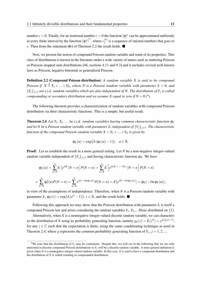
Definition 2.2 (Compound Poisson distribution) A random variable X is said to be compoundPoisson if X d
= Y1 + ...+YN , where N is a Poisson random variable with parameter λ > 0, andYj j≥1 are i.i.d. random variables which are also independent of N. The distribution of Yj is calledcompounding or secondary distribution and we assume X equal to zero if N = 0 (4).
The following theorem provides a characterization of random variables with compound Poissondistribution via their characteristic functions. This is a simple, but useful result.
Theorem 2.4 Let Y1, Y2, . . . be i.i.d. random variables having common characteristic function ϕY
and let N be a Poisson random variable with parameter λ , independent of Yj j≥1. The characteristicfunction of the compound Poisson random variable X = Y1 + ...+YN is given by
ϕX(u) = expλ (ϕY (u)−1), u ∈ R.
Proof: Let us establish the result in a more general setting. Let N be a non-negative integer-valuedrandom variable independent of Yj j≥1 and having characteristic function ϕN . We have
ϕX(u) =∞
∑n=0
E[eiuX |N = n
]P(N = n) =
∞
∑n=0
E[eiu(Y1+...+YN) |N = n
]P(N = n)
=∞
∑n=0
ϕnY (u)P(N = n) =
∞
∑n=0
ein(−i lnϕY (u))P(N = n) = E[eiN(−i lnϕY (u))] = ϕN(−i lnϕY (u)),
in view of the assumptions of independence. Therefore, when N is a Poisson random variable withparameter λ , ϕN(v) = expλ (eiv −1), v ∈ R, and the result holds.
Following this approach we may show that the Poisson distribution with parameter λ is itself acompound Poisson law and arises considering the random variables Y1, Y2,... Dirac distributed on 1.
Alternatively, when X is a nonnegative integer-valued discrete random variable, we can characteri-ze the distribution of X using its probability generating function, namely gX(z) = E(zX) = eλ (g(z)−1),for any z ∈ C such that the expectation is finite, using the same conditioning technique as used inTheorem 2.4, where g represents the common probability generating function of Yj, j = 1,2, ....
4We note that the distribution of Y j may be continuous. Despite this, we will see in the following that we are onlyinterested in discrete compound Poisson distributions so Y j will be a discrete random variable. A more general definition isgiven when N is a nonnegative integer-valued random variable. In this case, X is said to have a compound distribution andthe distribution of N is called counting or compounded distribution.

12 The compound Poisson integer-valued GARCH model
Remark 2.2 From Theorem 2.4, we can deduce that when E(Y 21 )< ∞, the mean and the variance of
X are given by E(X) =−iϕ ′X(0) = λE(Y1) and V (X) =−ϕ ′′
X(0)−λ 2[E(Y1)]2 = λE(Y 2
1 ). This meansthat, except when the compounding distribution is the Dirac law on 0 or the Dirac law on 1(hence X is Poisson distributed), all the nonnegative integer-valued compound Poisson distributionsare overdispersed, i.e., have variance larger than the mean, since
V (X)
E(X)=
E(Y 21 )
E(Y1)= 1+
E[Y1(Y1 −1)]E(Y1)
> 1.
Remark 2.3 The moments of any order m ≥ 1 of a compound Poisson distribution can be calculatedusing the closed-form formulae provided by Grubbström and Tang [39]. They stated that for acompound Poisson random variable X its m-th moment is given by
E(Xm) =m
∑r=0
1r!
E
[r−1
∏k=0
(N − k)
]r
∑k=0
(rk
)(−1)r−kE
[(k
∑j=1
Yj
)m], (2.1)
interpreting ∑kj=1Yj to be zero for k = 0. Since N follows a Poisson distribution with parameter λ its
r-th descending factorial moment is E[∏r−1k=0 (N − k)] = λ r, for r ≥ 1 [46, p. 161]. (5)
We now give some examples of compound Poisson laws which are relevant in the following:the negative binomial, the generalized Poisson, the Neyman type-A and the geometric Poissondistributions. More examples can be found in [46, chap. 9].
Example 2.2 (Negative binomial distribution) Given r ∈N and p∈]0,1[, let Yj j≥1 be a sequenceof i.i.d. logarithmic random variables with parameter 1− p, i.e., with probability mass function
P(Yj = y) =−(1− p)y
y ln p, y = 1,2, . . . ,
and let N be a random variable independent of Yj j≥1 and having Poisson law with mean −r ln p.Then X = Y1 + ...+YN follows a negative binomial (NB for brevity) law with parameters (r, p), i.e.,
P(X = x) =
(x+ r−1
r−1
)pr(1− p)x, x = 0,1, ...
Indeed, from Theorem 2.4, the characteristic function of X has the form
ϕX(u) = exp−r[ln(1− (1− p)eiu)− ln p]=(
p1− (1− p)eiu
)r
,
since λ = −r ln p and ϕ(u) = ln(1− (1− p)eiu)/ ln p (which is the characteristic function of thelogarithmic distribution). So, the NB(r, p) distribution (and also the geometric(p) as particular casewhen r = 1) belongs to the class of compound Poisson distributions. We observe that
E(Y1) =−1− pp ln p
, E(Y 21 ) =− 1− p
p2 ln p, E(X) =
r(1− p)p
, and V (X) =r(1− p)
p2 .
5In fact, Grubbström and Tang [39] proved that formula (2.1) is valid for any compound distribution.
2.1 Infinitely divisible distributions and their fundamental properties 13
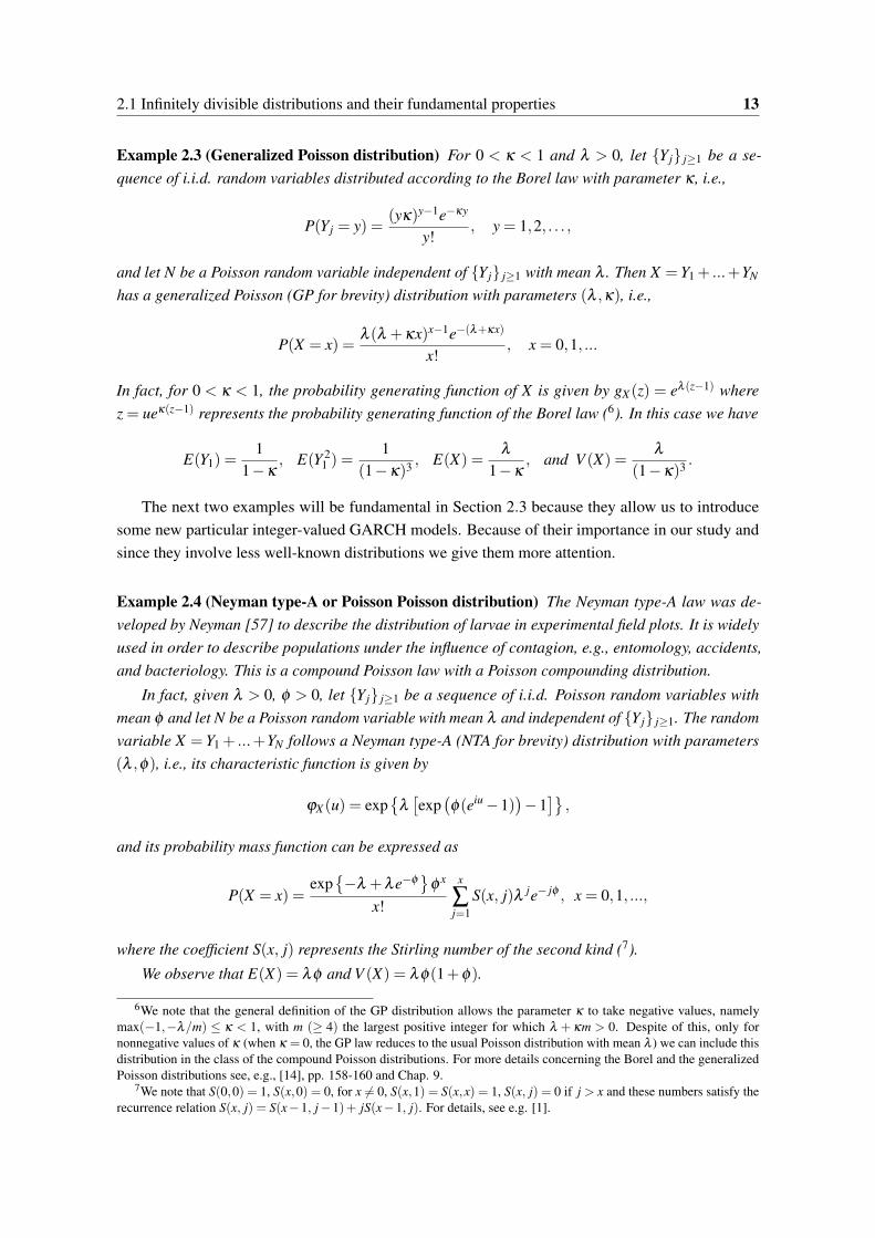
Example 2.3 (Generalized Poisson distribution) For 0 < κ < 1 and λ > 0, let Yj j≥1 be a se-quence of i.i.d. random variables distributed according to the Borel law with parameter κ , i.e.,
P(Yj = y) =(yκ)y−1e−κy
y!, y = 1,2, . . . ,
and let N be a Poisson random variable independent of Yj j≥1 with mean λ . Then X = Y1 + ...+YN
has a generalized Poisson (GP for brevity) distribution with parameters (λ ,κ), i.e.,
P(X = x) =λ (λ +κx)x−1e−(λ+κx)
x!, x = 0,1, ...
In fact, for 0 < κ < 1, the probability generating function of X is given by gX(z) = eλ (z−1) wherez = ueκ(z−1) represents the probability generating function of the Borel law (6). In this case we have
E(Y1) =1
1−κ, E(Y 2
1 ) =1
(1−κ)3 , E(X) =λ
1−κ, and V (X) =
λ
(1−κ)3 .
The next two examples will be fundamental in Section 2.3 because they allow us to introducesome new particular integer-valued GARCH models. Because of their importance in our study andsince they involve less well-known distributions we give them more attention.
Example 2.4 (Neyman type-A or Poisson Poisson distribution) The Neyman type-A law was de-veloped by Neyman [57] to describe the distribution of larvae in experimental field plots. It is widelyused in order to describe populations under the influence of contagion, e.g., entomology, accidents,and bacteriology. This is a compound Poisson law with a Poisson compounding distribution.
In fact, given λ > 0, φ > 0, let Yj j≥1 be a sequence of i.i.d. Poisson random variables withmean φ and let N be a Poisson random variable with mean λ and independent of Yj j≥1. The randomvariable X = Y1 + ...+YN follows a Neyman type-A (NTA for brevity) distribution with parameters(λ ,φ), i.e., its characteristic function is given by
ϕX(u) = exp
λ[exp(φ(eiu −1)
)−1]
,
and its probability mass function can be expressed as
P(X = x) =exp−λ +λe−φ
φ x
x!
x
∑j=1
S(x, j)λ je− jφ , x = 0,1, ...,
where the coefficient S(x, j) represents the Stirling number of the second kind (7).
We observe that E(X) = λφ and V (X) = λφ(1+φ).
6We note that the general definition of the GP distribution allows the parameter κ to take negative values, namelymax(−1,−λ/m) ≤ κ < 1, with m (≥ 4) the largest positive integer for which λ + κm > 0. Despite of this, only fornonnegative values of κ (when κ = 0, the GP law reduces to the usual Poisson distribution with mean λ ) we can include thisdistribution in the class of the compound Poisson distributions. For more details concerning the Borel and the generalizedPoisson distributions see, e.g., [14], pp. 158-160 and Chap. 9.
7We note that S(0,0) = 1, S(x,0) = 0, for x = 0, S(x,1) = S(x,x) = 1, S(x, j) = 0 if j > x and these numbers satisfy therecurrence relation S(x, j) = S(x−1, j−1)+ jS(x−1, j). For details, see e.g. [1].

14 The compound Poisson integer-valued GARCH model
From [46, Section 9.6], when φ is small X is approximately distributed as a Poisson variablewith mean λφ and if λ is small X is approximately distributed as a zero-inflated Poisson (ZIP forbrevity, see Section 5.1) variable with parameters (φ ,1−λ ). We illustrate these properties with thegraph present in Figure 2.1, where we represent the probability mass function (p.m.f.) of the NTAdistribution considering different values for the parameters (λ ,φ).
Fig. 2.1 Probability mass function of X ∼ NTA(λ ,φ). From the top to the bottom in abscissax = 2, (λ ,φ) = (10,0.1) (approximately Poisson(1), with p.m.f. represented in blue), (4,1), (0.3,4)(approximately ZIP(4,0.7), with p.m.f. represented in red).
Example 2.5 (Geometric Poisson or Pólya-Aeppli distribution) The geometric Poisson law wasdescribed by Pólya [63] and has been applied to a variety of biological data, in the control of defectsin software or in traffic accident data (8). This is an example of a compound Poisson law with ageometric compounding distribution. Indeed, given λ > 0 and p ∈]0,1[ let Yj j≥1 be a sequence ofi.i.d. geometric random variables with parameter p, i.e., with probability mass function
P(Yj = y) = p(1− p)y, y = 0,1, . . . ,
and let N be a Poisson random variable with parameter λ
1−p and independent of Yj j≥1. Therandom variable X =Y1 + ...+YN follows a geometric Poisson (GEOMP for brevity) distribution withparameters (λ , p), i.e., its characteristic function is given by
ϕX(u) = exp
λ
(eiu −1
1− (1− p)eiu
),
and its probability mass function can be expressed as
P(X = 0) = e−λ ,
8For more details see, e.g., [46, Section 9.7] or [59].

2.1 Infinitely divisible distributions and their fundamental properties 15
P(X = x) =x
∑n=1
e−λ λ n
n!
(x−1n−1
)pn(1− p)x−n, x = 1,2, ...
We observe that E(X) = λ/p, V (X) = λ (2− p)/p2 and when p = 1 the geometric Poissondistribution reduces to the Poisson law with parameter λ . In Figure 2.2, we represent the probabilitymass function of the GEOMP distribution considering different values for the parameters (λ , p).
Fig. 2.2 Probability mass function of X ∼ GEOMP(λ , p) with λ/p = 10 and p taking several values.From the top to the bottom in abscissa x = 10, p equals 1, 0.8, 0.6, 0.4, 0.2.
Let us now prove that a compound Poisson distribution is infinitely divisible. From Theorem2.4, we know that if X is a compound Poisson random variable then its characteristic functionhas the form ϕX(u) = expλ (ϕ(u)− 1), u ∈ R, for some λ > 0 and ϕ a characteristic function.Then, for any n ∈ N, ϕX can be represented as ϕX(u) = [ϕn(u)]n with ϕn(u) = exp
λ
n (ϕ(u)−1)
the characteristic function of the random variable Y1 + ...+YNn , where the random variable Nn hasthe Poisson distribution with parameter λ/n and is independent of the random variables Y1, Y2,...Therefore compound Poisson distributions belong to the class of infinitely divisible distributions.
Although the converse of this statement is not true, all the infinitely divisible distributions may beobtained from the family of compound Poisson as stated in the following theorem whose proof can befound in Gnedenko and Kolmogorov [31, p. 74].
Theorem 2.5 The class of infinitely divisible distributions coincides with the class of the compoundPoisson laws and of limits of these laws in the sense of the weak convergence.
As, in this work, we are developing models for the study of time series of counts, we nowconcentrate our attention on the set of the nonnegative integer-valued discrete infinitely divisible laws.
Generally a nonnegative integer-valued discrete random variable X is called infinitely divisiblewhen, according to Definition 2.1, Yn, j, j = 1, ...,n, are i.i.d. nonnegative integer-valued discreterandom variables as well. Sometimes, to make a clear distinction, X is said to be "discretely infinite
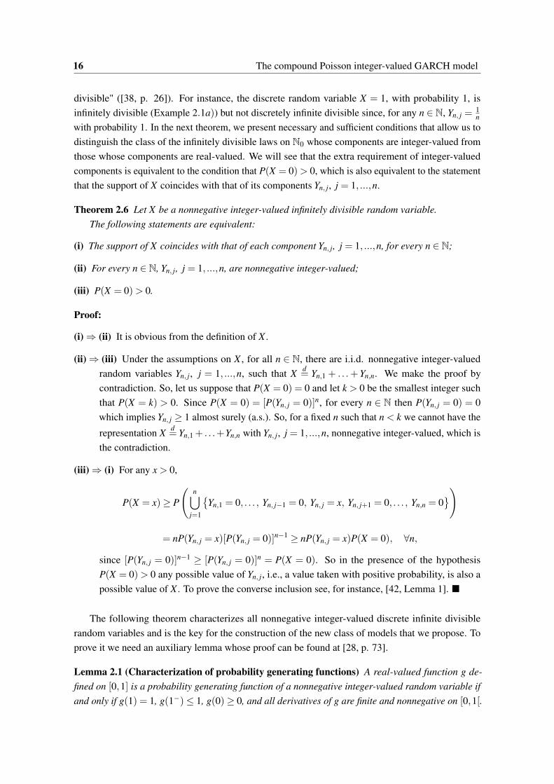
16 The compound Poisson integer-valued GARCH model
divisible" ([38, p. 26]). For instance, the discrete random variable X = 1, with probability 1, isinfinitely divisible (Example 2.1a)) but not discretely infinite divisible since, for any n ∈ N, Yn, j =
1n
with probability 1. In the next theorem, we present necessary and sufficient conditions that allow us todistinguish the class of the infinitely divisible laws on N0 whose components are integer-valued fromthose whose components are real-valued. We will see that the extra requirement of integer-valuedcomponents is equivalent to the condition that P(X = 0)> 0, which is also equivalent to the statementthat the support of X coincides with that of its components Yn, j, j = 1, ...,n.
Theorem 2.6 Let X be a nonnegative integer-valued infinitely divisible random variable.The following statements are equivalent:
(i) The support of X coincides with that of each component Yn, j, j = 1, ...,n, for every n ∈ N;
(ii) For every n ∈ N, Yn, j, j = 1, ...,n, are nonnegative integer-valued;
(iii) P(X = 0)> 0.
Proof:
(i) ⇒ (ii) It is obvious from the definition of X .
(ii) ⇒ (iii) Under the assumptions on X , for all n ∈ N, there are i.i.d. nonnegative integer-valuedrandom variables Yn, j, j = 1, ...,n, such that X d
= Yn,1 + . . .+Yn,n. We make the proof bycontradiction. So, let us suppose that P(X = 0) = 0 and let k > 0 be the smallest integer suchthat P(X = k) > 0. Since P(X = 0) = [P(Yn, j = 0)]n, for every n ∈ N then P(Yn, j = 0) = 0which implies Yn, j ≥ 1 almost surely (a.s.). So, for a fixed n such that n < k we cannot have the
representation X d= Yn,1 + . . .+Yn,n with Yn, j, j = 1, ...,n, nonnegative integer-valued, which is
the contradiction.
(iii) ⇒ (i) For any x > 0,
P(X = x)≥ P
(n⋃
j=1
Yn,1 = 0, . . . , Yn, j−1 = 0, Yn, j = x, Yn, j+1 = 0, . . . , Yn,n = 0
)
= nP(Yn, j = x)[P(Yn, j = 0)]n−1 ≥ nP(Yn, j = x)P(X = 0), ∀n,
since [P(Yn, j = 0)]n−1 ≥ [P(Yn, j = 0)]n = P(X = 0). So in the presence of the hypothesisP(X = 0)> 0 any possible value of Yn, j, i.e., a value taken with positive probability, is also apossible value of X . To prove the converse inclusion see, for instance, [42, Lemma 1].
The following theorem characterizes all nonnegative integer-valued discrete infinite divisiblerandom variables and is the key for the construction of the new class of models that we propose. Toprove it we need an auxiliary lemma whose proof can be found at [28, p. 73].
Lemma 2.1 (Characterization of probability generating functions) A real-valued function g de-fined on [0,1] is a probability generating function of a nonnegative integer-valued random variable ifand only if g(1) = 1, g(1−)≤ 1, g(0)≥ 0, and all derivatives of g are finite and nonnegative on [0,1[.

2.2 The definition of the CP-INGARCH model 17
Theorem 2.7 Let X be a nonnegative integer-valued random variable such that 0 < P(X = 0)< 1.Then, X is infinitely divisible if and only if X has a compound Poisson distribution.
Proof: We need only to prove the necessary condition of infinite divisibility. So, let g be theprobability generating function of X which is infinitely divisible. We note that 0 < g(0)< 1. Then, forevery n ∈ N, gn = g1/n is a probability generating function. Let us define the function h in the form
hn(z) =gn(z)−gn(0)
1−gn(0)= 1− 1−g(z)1/n
1−g(0)1/n .
Since hn(0) = 0, hn(1) = 1 (because gn(1) = 1), hn(1−)≤ 1 and there exist all the derivatives of
hn, namely h(k)n (z) = g(k)n (z)1−gn(0)
, which are nonnegative in [0,1[ because 1− gn(0) > 0, then from theprevious lemma hn is a probability generating function.
Letting n → ∞ and using the fact that lnα = limn→∞ n(α1/n −1) for α > 0, we have
limn→∞
hn(z) = 1− limn→∞
n(−1+g(z)1/n)
n(−1+g(0)1/n)= 1− lng(z)
lng(0)= h(z),
and then from the continuity theorem (9) we conclude that the function h is a probability generatingfunction. Then, it follows that g(z) = expλ (h(z)− 1) with λ = − lng(0), i.e., g is a probabilitygenerating function of a compound Poisson distribution, which concludes the proof.
Let us note that any nonnegative integer-valued compound Poisson random variable X assumes thevalue zero with positive probability, namely, P(X = 0) = gX(0) = e−λ (1−g(0)), which is in accordancewith the hypothesis of the previous theorems.
2.2 The definition of the CP-INGARCH model
Let X = (Xt , t ∈ Z) be a nonnegative integer-valued stochastic process and, for any t ∈ Z, let X t−1 bethe σ -field generated by Xt−s,s ≥ 1.
Definition 2.3 (CP-INGARCH(p, q) model) The process X is said to follow a compound Poissoninteger-valued GARCH model with orders p and q (where p,q ∈ N), briefly a CP-INGARCH(p,q), if,for all t ∈ Z, the characteristic function of Xt conditioned on X t−1 is given by
ΦXt |X t−1(u) = exp
i
λt
ϕ ′t (0)
[ϕt(u)−1], u ∈ R, (2.2)
with
E(Xt |X t−1) = λt = α0 +p
∑j=1
α jXt− j +q
∑k=1
βkλt−k, (2.3)
9Let Xnn∈N be a sequence of nonnegative integer-valued random variables with Xn having probability generatingfunction gn. If Xn converges weakly to X then limn→∞ gn(z) = gX (z) for 0 ≤ z ≤ 1. Conversely, if limn→∞ gn(z) = g(z)for 0 ≤ z ≤ 1 with g a function that is (left-) continuous at one, then g is the probability generating function of a randomvariable X and Xn converges weakly to X . See, for example, [73, p. 489].
18 The compound Poisson integer-valued GARCH model
for some constants α0 > 0, α j ≥ 0 ( j = 1, ..., p), βk ≥ 0 (k = 1, ...,q), and where (ϕt , t ∈ Z) is afamily of characteristic functions on R, X t−1-measurables, associated to a family of discrete lawswith support in N0 and finite mean (10). i represents the imaginary unit.
If q = 1 and β1 = 0, the CP-INGARCH(p,q) model is simply denoted by CP-INARCH(p).
Assuming that the functions (ϕt , t ∈ Z) are twice differentiable at zero, in addition to the condi-tional expectation λt we can also specify the evolution of the conditional variance of X as
V (Xt |X t−1) =−Φ′′Xt |X t−1
(0)−λ2t =−i
ϕ ′′t (0)
ϕ ′t (0)
λt . (11)
Remark 2.4 The CP-INGARCH model is able to capture different kinds of overdispersion. Thisresults from the fact that whenever the conditional distribution is overdispersed we deduce fromwell-known properties on conditional moments (12) that
V (Xt)
E(Xt)≥
E(V (Xt |X t−1))
E(Xt)>
E(E(Xt |X t−1))
E(Xt)= 1;
moreover, if we have a conditional Poisson distribution the corresponding unconditional law isoverdispersed as V (Xt) = E(λt)+V (λt)> E(Xt), whenever we have conditional heteroscedasticity.
Similarly to what was established by Bollerslev [10] for the GARCH model, it is possible, in somecases, to state a CP-INARCH(∞) representation of the CP-INGARCH(p,q) process, i.e., Xt may bewritten explicitly as a function of its infinite past. With this goal, let us consider the polynomials Aand B of degrees p and q given, respectively, by
A(L) = α1L+ ...+αpLp,
B(L) = 1−β1L− ...−βqLq,
whose coefficients are those presented in equation (2.3) and L is the backshift operator (13). Further-more, to ensure the existence of the inverse B−1 of B, let us suppose that the roots of B(z) = 0 lieoutside the unit circle. In fact, under this assumption, we can write
B(L) = 1−q
∑j=1
β jL j =q
∏j=1
(1− L
z j
)10We note that, as ϕt is the characteristic function of a discrete distribution with support in N0 and finite mean, the
derivative of ϕt(u) at u = 0, ϕ ′t (0), exists and is nonzero.
11We observe that
Φ′Xt |X t−1
(u) = iϕ ′
t (u)λt
ϕ ′t (0)
exp
iλt
ϕ ′t (0)
[ϕt(u)−1],
Φ′′Xt |X t−1
(u) =
[iϕ ′′
t (u)λt
ϕ ′t (0)
−(
ϕ ′t (u)λt
ϕ ′t (0)
)2]
exp
iλt
ϕ ′t (0)
[ϕt(u)−1], u ∈ R.
12E(Xt) = E[E(Xt |X t−1)] and V (Xt) = E[V (Xt |X t−1)]+V [E(Xt |X t−1)].13For any integer j, L jXt = Xt− j.

2.2 The definition of the CP-INGARCH model 19
where z1, ...,zq are the roots of the polynomial B(L). From this equality it follows that B(L) will beinvertible if the polynomial 1− L
z jis invertible, for all j ∈ 1, ...,q. But 1−θL is invertible if and
only if |θ | = 1 ([36]) and thus, if we assume |z j|> 1, for all j ∈ 1, ...,q, then B(L) is invertible (14).
Let us consider in the following the Hypothesis H1:q
∑j=1
β j < 1.
Lemma 2.2 The roots of the polynomial B(z) = 1−β1z− ...−βqzq, with nonnegative β j, j = 1, ...,q,lie outside the unit circle if and only if the coefficients β j satisfy the hypothesis H1.
Proof: If ∑qj=1 β j ≥ 1, then B(1)≤ 0. As B(0) = 1 > 0 and B(z) is a continuous function in [0,1],
then there is a real root of B(z) in the interval ]0,1]. On the other hand, if ∑qj=1 β j < 1, let us suppose
by contradiction that there is at least a root z0 of B(z) such that |z0| ≤ 1. Under these conditions,
B(z0) = 0 ⇔ 1−q
∑i=1
β jzj0 = 0 ⇔ 1 =
q
∑j=1
β jzj0 =
∣∣∣∣∣ q
∑j=1
β jzj0
∣∣∣∣∣≤ q
∑j=1
β j |z0| j ≤q
∑j=1
β j,
so 1 ≤ ∑qj=1 β j < 1, which is a contradiction.
So, given the polynomials A(L) and B(L), and assuming the hypothesis H1, we can rewrite theconditional expectation (2.3) in the form
B(L)λt = α0 +A(L)Xt ⇔ λt = B−1(L)[α0 +A(L)Xt ]
⇔ λt = α0B−1(1)+H(L)Xt ,
with H(L) = B−1(L)A(L) = ∑∞j=1 ψ jL j, where ψ j is the coefficient of z j in the Maclaurin expansion
of the rational function A(z)/B(z), that is,
ψ j =
α1, if j = 1,
α j +j−1
∑k=1
βkψ j−k, if 2 ≤ j ≤ p,
q
∑k=1
βkψ j−k, if j ≥ p+1,
and then, denoting α0B−1(1) as ψ0, we get
λt = ψ0 +∞
∑j=1
ψ jXt− j, (2.4)
which together with (2.2) expresses a CP-INARCH(∞) representation of the model in study. Thisrepresentation will be useful in the construction of a solution of the model presented in Section 3.4.
14We note that for B(L) to have inverse it is sufficient that the roots of B(z) = 0 are, in module, different from 1. However,in what follows we will consider them outside the unit circle, since this condition will allow us to express the conditionalexpectation λt only in terms of the past information of Xt .
20 The compound Poisson integer-valued GARCH model
2.3 Important cases - known and new models
The functional form of the conditional characteristic function (2.2) allows a wide flexibility of theclass of compound Poisson INGARCH models. In fact, as we assume that the family of discretecharacteristic functions (ϕt , t ∈Z) (respectively, the associated laws of probability) is X t−1-measurableit means that its elements may be random functions (respectively, random measures) or deterministicones. So, it is not surprising that this new model includes a lot of recent contributions on integer-valuedtime series modeling as well as several new processes.
To illustrate the large class of models enclosed in this framework, let us recall that since theconditional distribution of Xt is a discrete compound Poisson law with support in N0 then, for all t ∈ Zand conditioned on X t−1, Xt can be identified in distribution with the random sum
Xtd= Xt,1 +Xt,2 + . . .+Xt,Nt , (2.5)
where Nt is a random variable following a Poisson distribution with parameter λ ∗t = λt/E(Xt, j), and
Xt,1, Xt,2, ... are discrete and independent random variables, with support contained in N0, independentof Nt and having common characteristic function ϕt , with finite mean.
Some concrete examples that fall in the preceding framework are discussed in the following.
1. The INGARCH model [25] corresponds to a CP-INGARCH model considering λ ∗t = λt and ϕt
the characteristic function of the Dirac’s law concentrated in 1, i.e., ϕt(u) = eiu, u ∈ R.
2. Inspired by the INGARCH model, Zhu [81] proposed the negative binomial INGARCH(p,q)process (NB-INGARCH for brevity), defined as
Xt | X t−1 ∼ NB(
r,1
1+λt
), λt = α0 +
p
∑j=1
α jXt− j +q
∑k=1
βkλt−k,
with r ∈ N, α0 > 0, α j ≥ 0, βk ≥ 0, j = 1, ..., p, k = 1, ...,q. We observe that in this modelE(Xt |X t−1) = rλt and V (Xt |X t−1) = rλt(1+λt).
Considering in the representation (2.5), the random variables Xt, j, j = 1,2, ..., having a loga-rithmic distribution with parameter λt
1+λtand λ ∗
t = r ln(1+λt) (see Example 2.2) we recover,unless a scale factor, the NB-INGARCH(p,q) model.
3. To handle both conditional over-, equi- and underdispersion, Zhu [82] introduced a generalizedPoisson INGARCH(p,q) process (GP-INGARCH for brevity) by considering
Xt | X t−1 ∼ GP((1−κ)λt ,κ) , λt = α0 +p
∑j=1
α jXt− j +q
∑k=1
βkλt−k,
where α0 > 0, α j ≥ 0, βk ≥ 0, j = 1, ..., p, k = 1, ...,q and max−1,−(1−κ)λt/4 < κ < 1.In this case we have E(Xt |X t−1) = λt and V (Xt |X t−1) = λt/(1−κ)2.
For 0 < κ < 1, we recover the GP-INGARCH(p,q) model from the CP-INGARCH(p,q)considering that in the representation (2.5) the common distribution of the random variablesXt, j, j = 1,2, ..., is the Borel law with parameter κ and λ ∗
t = (1−κ)λt (see Example 2.3).

2.3 Important cases - known and new models 21
4. Xu et al. [80] recently proposed the family of dispersed INARCH models (DINARCH forbrevity) to deal with different types of conditional dispersion assuming that the conditionalvariance is equal to the conditional expectation multiplied by a constant α > 0. As a particularcase of this model, they present the NB-DINARCH(p) for which the conditional law is anegative binomial one, where the random parameter is the order of occurrences and not itsprobability as in the NB-INARCH(p) of Zhu [81]; namely they considered
Xt | X t−1 ∼ NB(
λt
α −1,
1α
), λt = α0 +
p
∑j=1
α jXt− j,
with α > 1, α0 > 0, α j ≥ 0, j = 1, ..., p. We note that E(Xt |X t−1) = λt and V (Xt |X t−1) = αλt .This process results from the CP-INARCH(p) model considering in the representation (2.5)the random variables Xt, j with a logarithmic law with parameter α−1
αand λ ∗
t =− λtα−1 ln
( 1α
).
In the NB-INGARCH model (case 2) the parameter involved in the distribution of the randomvariables Xt, j, j = 1,2, ..., depends on λt , and thus depends on the previous observations of the process;so, it is a clear example of a CP-INGARCH model where the characteristic function ϕt is a randomfunction. In the other particular CP-INGARCH models presented (cases 1, 3 and 4) the law of therandom variables Xt, j have the same parameter for every t ∈ Z (1, κ and α−1
α, respectively). So, in the
INGARCH, GP-INGARCH and NB-DINARCH models, the characteristic function ϕt is deterministicand independent of t. For that reason, in such cases we will refer these functions simply as ϕ .
Specifying the distribution of the random variables Xt, j, j = 1,2, ..., in representation (2.5) enablesus to find new interesting models as, for instance, the GEOMP-INGARCH and the NTA-INGARCHones. We note that these new models are naturally interesting in practice as the associated conditionaldistributions, namely the geometric Poisson and the Neyman type-A, explain phenomena in variousareas of application (recall Examples 2.4 and 2.5).
In the following examples we present some of these new models in which we also find situationswhere (ϕt , t ∈ Z) is a family of dependent on t deterministic characteristic functions (namely case 7).
5. Let us define a geometric Poisson INGARCH(p,q) model (GEOMP-INGARCH) as
Xt | X t−1 ∼ GEOMP(
rλt
λt + r,
rλt + r
), λt = α0 +
p
∑j=1
α jXt− j +q
∑k=1
βkλt−k,
with r > 0, α0 > 0, α j ≥ 0, βk ≥ 0, j = 1, ..., p, k = 1, ...,q. Let us note that E(Xt |X t−1) = λt andV (Xt |X t−1) = λt
(1+ 2
r λt). Thus, if we consider in representation (2.5) the random variables
Xt, j, j = 1,2, ..., following the geometric distribution with parameter rr+λt
and λ ∗t = r we recover
this model, which means that it satisfies a CP-INGARCH model.
6. Let us consider independent random variables (Xt, j, t ∈ Z) following the same discrete distribu-tion with constant parameters, finite mean and support contained in N0. The process X definedby (2.5) with Nt independent of each Xt, j, j = 1,2, ..., and having a Poisson distribution withparameter λt/E(Xt, j) satisfies a CP-INGARCH model.

22 The compound Poisson integer-valued GARCH model
For instance, if we consider
(a) the geometric distribution with parameter p∗ ∈]0,1[ for Xt, j, j = 1,2, ..., and the parameterp∗λt
1−p∗ in the Poisson law of the variable Nt we obtain as conditional distribution
Xt | X t−1 ∼ GEOMP(p∗λt , p∗) , λt = α0 +p
∑j=1
α jXt− j +q
∑k=1
βkλt−k,
with α0 > 0, α j ≥ 0, βk ≥ 0, j = 1, ..., p, k = 1, ...,q. We observe that E(Xt |X t−1) = λt
and V (Xt |X t−1) = λt
(2−p∗
p∗
). This model will be denoted by GEOMP2-INGARCH(p,q)
to distinguish it from the model presented in case 5. In fact, although these two modelshave as conditional distribution the geometric Poisson law, the difference between themresults from the parameter of the geometric distribution which involves or not λt .
(b) the Poisson distribution with parameter φ > 0 for Xt, j, j = 1,2, ..., and the parameter λt/φ
in the Poisson distribution of Nt , we define the Neyman type-A INGARCH(p,q) model(NTA-INGARCH for brevity), that is,
Xt | X t−1 ∼ NTA(
λt
φ,φ
), λt = α0 +
p
∑j=1
α jXt− j +q
∑k=1
βkλt−k,
with α0 > 0, α j ≥ 0, βk ≥ 0, j = 1, ..., p, k = 1, ...,q.
We note that E(Xt |X t−1) = λt and V (Xt |X t−1) = λt (1+φ).
7. (a) Let (Xt, j, t ∈ Z) be independent random variables following a binomial distribution withparameters r ∈ N and e−|t|, that is, ϕt(u) =
(eiu−|t|+1− e−|t|)r
, u ∈ R, t ∈ Z, and let Nt
be an independent of Xt, j random variable following a Poisson distribution with parameterλt/re−|t|. The process X defined by (2.5) satisfies a CP-INGARCH model.
(b) Changing the success probability of the binomial distribution by (t2 + 1)−1, that is,considering the characteristic function ϕt(u) = ( eiu+t2
t2+1 )r, u ∈ R, t ∈ Z, and the mean ofthe Poisson law equal to λt(t2 +1)/r, the process X still satisfies a CP-INGARCH model.
Remark 2.5 We note that the pair (λ ∗t ,ϕt) is not uniquely determined by ΦXt |X t−1
, but it will happen,if we choose ϕt such that P(Xt, j = 0) = 0, what can always be done. In fact, modifying the probabilityat zero in the distribution of Xt, j, j = 1,2, ..., does not add a new conditional distribution because it isequivalent to modifying the parameter λ ∗
t in the Poisson distribution, [60, Theorem 5.11].
For example, let us consider the GEOMP2-INGARCH model. This process was obtained taking ϕt
the characteristic function of a geometric law with parameter p∗ and then λ ∗t = p∗λt
1−p∗ . But we can alsoobtain the same process considering ϕt the characteristic function of a shifted geometric law (15) withparameter p∗ and in this case λ ∗
t = p∗λt . Nevertheless, when we refer to the GEOMP2-INGARCHmodel it must be considered as it was initially defined. The same for the other models.
15The probability mass function of a random variable Y following a shifted geometric distribution with parameter p ∈]0,1[is given by P(Y = y) = p(1− p)y−1, for y = 1,2, . . . So, E(Y ) = 1/p and V (Y ) = (1− p)/p2.
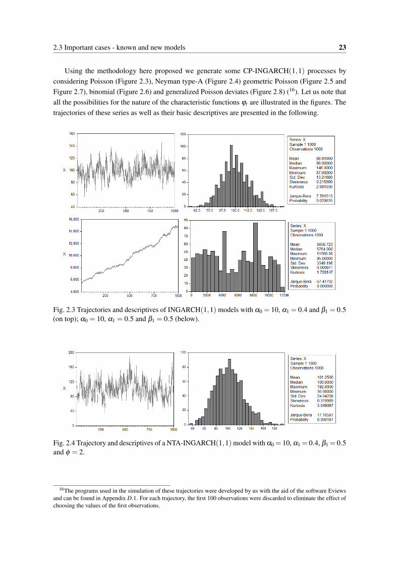
2.3 Important cases - known and new models 23
Using the methodology here proposed we generate some CP-INGARCH(1,1) processes byconsidering Poisson (Figure 2.3), Neyman type-A (Figure 2.4) geometric Poisson (Figure 2.5 andFigure 2.7), binomial (Figure 2.6) and generalized Poisson deviates (Figure 2.8) (16). Let us note thatall the possibilities for the nature of the characteristic functions ϕt are illustrated in the figures. Thetrajectories of these series as well as their basic descriptives are presented in the following.
Fig. 2.3 Trajectories and descriptives of INGARCH(1,1) models with α0 = 10, α1 = 0.4 and β1 = 0.5(on top); α0 = 10, α1 = 0.5 and β1 = 0.5 (below).
Fig. 2.4 Trajectory and descriptives of a NTA-INGARCH(1,1) model with α0 = 10, α1 = 0.4, β1 = 0.5and φ = 2.
16The programs used in the simulation of these trajectories were developed by us with the aid of the software Eviewsand can be found in Appendix D.1. For each trajectory, the first 100 observations were discarded to eliminate the effect ofchoosing the values of the first observations.

24 The compound Poisson integer-valued GARCH model
Fig. 2.5 Trajectory and descriptives of a GEOMP-INGARCH(1,1) model with α0 = 10, α1 = 0.4,β1 = 0.5 and r = 2.
Fig. 2.6 Trajectory and descriptives of a CP-INGARCH(1,1) model with ϕt the characteristic functionof a binomial(5000, 1
t2+1) distribution considering α0 = 10, α1 = 0.4, and β1 = 0.5.
Fig. 2.7 Trajectory and descriptives of a GEOMP2-INARCH(1) model with α0 = 10, α1 = 0.4, andp∗ = 0.3.
Fig. 2.8 Trajectory and descriptives of a GP-INARCH(1) model with α0 = 10, α1 = 0.4, and κ = 0.5.

2.3 Important cases - known and new models 25
Comparing the two trajectories presented in Figure 2.3 it is evident that the change made in thecoefficient α1 results in a non-stationary process, namely, in mean. So, it seems natural to think thatthe stationarity of the CP-INGARCH model is strongly related to the coefficients involved in theevolution of the conditional mean λt . The unconditional mean, when we consider the same coefficientsα0, α1 and β1, does not seem to be affected by the conditional distribution nor by the nature of thecharacteristic functions ϕt . In fact, it presents similar values when we compare the processes with thesame orders namely 99.819, 101.25, 99.461, 100.93 (figures 2.3 on top, 2.4, 2.5 and 2.6, respectively)and 17.183, 16.797 (figures 2.7 and 2.8, respectively).
The CP-INGARCH trajectories represented seem to concern processes with characteristics asoverdispersion, leptokurtosis (figures 2.5, 2.6, 2.7 and 2.8) and asymmetry around the mean. Wepoint out also the strong volatility in all the cases but especially in the NTA-INGARCH and GEOMP-INGARCH models.
The aim of the next chapter is to develop a unified and enlarged study on the probabilisticproperties within the class of the integer-valued GARCH models.


Chapter 3
Stationarity and Ergodicity in theCP-INGARCH process
An important property of a process is its stationarity or, in other words, its invariance under translationin time. In time series modeling, to evaluate stability properties over time is important particularlyin statistical developments for instance to reach good forecasts. Moreover, we are in conditions toanalyse all the characteristics of a process from a single (infinitely long) realisation when we have anergodic process. This is very important, since in the study of a time series only a single realizationfrom the series is available. Stationarity and ergodicity are then the two cornerstones on which thetime series analysis rests and they will be the subject of study in this chapter.
Necessary and sufficient conditions of first and second-order stationarity expressed in terms of thecoefficients of a CP-INGARCH(p,q) process are discussed respectively in Section 3.1 and 3.2, andillustrated by the study of some particular cases. Then, in Section 3.3, we obtain its autocorrelationfunction and we investigate the existence of higher-order moments when p = q = 1. We finish thechapter establishing a necessary and sufficient condition to ensure the strict stationarity and theergodicity of the CP-INGARCH(p,q) process. We should remark that the assumptions considered onthe family of characteristic functions to establish these properties concern a huge class of processes.
3.1 First-order stationarity
The following theorem is the starting point for establishing the weak stationarity for the CP-INGARCHprocess in the next section. We notice that the result obtained is not affected by the form of theconditional distribution but mainly by the evolution of λt specified in (2.3).
Theorem 3.1 Let X be a process satisfying the CP-INGARCH(p,q) model as specified in (2.2) and(2.3). This process is first-order stationary if and only if
p
∑j=1
α j +q
∑k=1
βk < 1.
27

28 Stationarity and Ergodicity in the CP-INGARCH process
Proof: To establish the first-order stationarity we should prove that E(Xt) exists and is independentof t, for any t ∈ Z. As Xt is a positive measurable function, we can write formally
µt = E(Xt) = E(E(Xt |X t−1)) = E(λt) = E
(α0 +
p
∑j=1
α jXt− j +q
∑k=1
βkλt−k
)
⇔ µt = α0 +p
∑j=1
α jµt− j +q
∑k=1
βkµt−k,
taking into account that the involved sums exist although they may be non finite. This non-homogeneous difference equation has a stable solution, which is finite and independent of t, ifand only if all roots z1, ..., zmax(p,q) of the equation 1−∑
pj=1 α jz j −∑
qk=1 βkzk = 0 lie outside the unit
circle, that is, if and only if ∑pj=1 α j +∑
qk=1 βk < 1.
Remark 3.1 As a consequence of the Theorem 3.1, provided that ∑pj=1 α j+∑
qk=1 βk < 1, the processes
λ = (λt , t ∈ Z) and X are both first-order stationary and its common unconditional mean is
E(Xt) = E(λt) = µ =α0
1−∑pj=1 α j −∑
qk=1 βk
.
From Theorem 3.1 we have assured that if the sum of the parameters α j’s and βk’s, j = 1, ..., p,k = 1, ...,q, is greater than or equal to 1 then the process X is not first-order stationary and, obviously,it will also not be a weakly stationary process. The second trajectory presented in Figure 2.3 is anINGARCH(1,1) process where the sum of the parameters α1 and β1 is equal to 1 and, as referredbefore, it is an example of a non-stationary process.
Moreover, we will see later that the condition of first-order stationarity displayed is also a necessaryand sufficient condition to obtain a strictly stationary solution of this model.
3.2 Weak stationarity
In this section, we analyse weak stationarity conditions for the CP-INGARCH(p,q) model. With thisgoal and in order to assure the existence of the corresponding distribution variance, we assume inwhat follows that the family of characteristic functions (ϕt , t ∈ Z) is twice differentiable.
The general class of models considered and the complexity in the study of the weak stationarity inthis class leads us to fix ourselves in the subclass of the CP-INGARCH(p,q) models for which thecharacteristic functions ϕt satisfy the following condition:
Hypothesis H2 : − iϕ ′′
t (0)ϕ ′
t (0)= v0 + v1λt ,
with v0 ≥ 0, v1 ≥ 0, not simultaneously zero. We note thatV (Xt |X t−1)
E(Xt |X t−1)=−i
ϕ ′′t (0)
ϕ ′t (0)
.
Despite the restriction, a quite general subclass is considered containing both random and deter-ministic characteristic functions ϕt . Recalling the variance of the involved conditional distributions,many of the examples presented in Section 2.3 can be included in this subclass. Namely,

3.2 Weak stationarity 29
• INGARCH(p,q) model with v0 = 1;
• GP-INGARCH(p,q) model with v0 =1
(1−κ)2 ;
• NB-DINARCH(p) model with v0 = α;
• GEOMP2-INGARCH(p,q) model with v0 =2− p∗
p∗;
• NTA-INGARCH(p,q) model with v0 = 1+φ ,
all of them with v1 = 0, and also the
• NB-INGARCH(p,q) model with v0 = v1 = 1;
• GEOMP-INGARCH(p,q) model with v0 = 1 and v1 =2r
.
Let us note that all the characteristic functions ϕt which are deterministic and independent of tsatisfy the hypothesis H2 since they imply v1 = 0.
Remark 3.2 Let us consider a real function k such that k′(0)/k(0) = 1. Considering
−iϕ ′′
t (u)ϕ ′
t (u)= (v0 + v1λt)
k′(u)k(u)
, u ∈ R,
we may writeddu
(−i ln(ϕ ′
t (u))+θ(t))= (v0 + v1λt)
k′(u)k(u)
which implies−i ln(ϕ ′
t (u))+θ(t) = (v0 + v1λt) ln(k(u))+ ζ (t)
and soϕ′t (u) = expi(v0 + v1λt) ln(k(u))+ζ (t), u ∈ R.
Thus the following general class of characteristic functions ϕt such that
ϕt(u) = eζ (t)∫
k(u)i(v0+v1λt)du+δ (t), u ∈ R,
is solution of H2. For instance, the characteristic function ϕ(u) = eiu, u ∈ R, can be written in thisform with v0 = 1, v1 = 0 and considering k(u) = eu, δ (t) = 0 and ζ (t) = ln i.
Remark 3.3 As noted in Remark 2.2, the family of conditional distributions considered can be equi-or overdispersed. Despite this, some of the next results are not restricted to these cases. In fact,we observe that when v1 = 0 the hypothesis H2 allows conditional underdispersion since the ratiobetween the conditional variance and the conditional mean, which corresponds to v0, can be in ]0,1[.Thus, the DINARCH(p) model proposed by Xu et al. [80] is also included in this study.
30 Stationarity and Ergodicity in the CP-INGARCH process
In order to obtain a necessary and sufficient condition of weak stationarity we begin by establishinga vectorial state space representation of X . To accomplish this let us observe that
E(Xt− jλt−k) = E[E(Xt− j|X t− j−1)λt−k
]= E(λt− jλt−k), if k ≥ j, (3.1)
E(Xt− jλt−k) = E [Xt− jE(Xt−k|X t−k−1)] = E(Xt− jXt−k), if k < j, (3.2)
from which we can deduce the expressions
E(XtXt−h) = E [E(Xt |X t−1)Xt−h] = E(λtXt−h)
= E
([α0 +
p
∑j=1
α jXt− j +q
∑k=1
βkλt−k
]Xt−h
)
= α0E (Xt−h)+p
∑j=1
α jE (Xt− jXt−h)+q
∑k=1
βkE (λt−kXt−h)
= α0E (Xt−h)+p
∑j=1
α jE (Xt− jXt−h)+h−1
∑k=1
βkE(Xt−kXt−h)+q
∑k=h
βkE(λt−kλt−h), h ≥ 1, (3.3)
and in a similar way
E(λtλt−h) = E
([α0 +
p
∑j=1
α jXt− j +q
∑k=1
βkλt−k
]λt−h
)
= α0E (λt−h)+p
∑j=1
α jE (Xt− jλt−h)+q
∑k=1
βkE (λt−kλt−h)
= α0E (λt−h)+h
∑j=1
α jE (λt− jλt−h)+p
∑j=h+1
α jE(Xt− jXt−h)+q
∑k=1
βkE (λt−kλt−h), h ≥ 0. (3.4)
Proposition 3.1 Let X be a first-order stationary process following a CP-INGARCH(p,q) modelsuch that H2 is satisfied. The vector Wt , t ∈ Z, of dimension p+q−1 given by
Wt =
E(X2t )
E(XtXt−1)
· · ·E(XtXt−(p−1))
E(λtλt−1)
· · ·E(λtλt−(q−1))
satisfies an autoregressive equation of order max(p,q):
Wt = B0 +max(p,q)
∑k=1
BkWt−k, (3.5)
where B0 is a real vector of dimension p+ q− 1 and Bk (k = 1, ...,max(p,q)) are real squaredmatrices of order p+q−1.

3.2 Weak stationarity 31
Proof: We begin noting that E(X2t ), E(XtXt−k) and E(λtλt−k) are not necessarily finite but, as
we have positive and measurable functions, we may apply the operator expectation E. For sake ofsimplicity, we focus the proof on the case p = q since the other cases can be obtained from this oneby setting additional parameters to 0.
Let us start by calculating E(X2t ) for any t ∈ Z. We have E(X2
t ) = E[E(X2t |X t−1)] and
E(X2t |X t−1) =V (Xt |X t−1)+ [E(Xt |X t−1)]
2 =−iϕ ′′
t (0)ϕ ′
t (0)λt +λ
2t = v0λt +(1+ v1)λ
2t
= v0
[α0 +
p
∑j=1
α jXt− j +p
∑k=1
βkλt−k
]+(1+ v1)
[α
20 +2α0
(p
∑j=1
α jXt− j +p
∑k=1
βkλt−k
)
+
(p
∑j=1
α jXt− j
)2
+2p
∑j=1
α jXt− j
p
∑k=1
βkλt−k +
(p
∑k=1
βkλt−k
)2
= v0α0 +(1+ v1)α20 +[v0 +2α0(1+ v1)]
(p
∑j=1
α jXt− j +p
∑k=1
βkλt−k
)+(1+ v1)
[p
∑j=1
α2j X2
t− j
+p
∑j,k=1j =k
α jαkXt− jXt−k +2p
∑j=1
p
∑k=1
α jβkλt−kXt− j +p
∑j=1
β2j λ
2t− j +
p
∑j,k=1j =k
β jβkλt− jλt−k
.So, using the first-order stationary hypothesis, we conclude
E(X2t ) = C+(1+ v1)
p
∑j=1
α2j E(X2
t− j)+p
∑j,k=1j =k
α jαkE(Xt− jXt−k)
+2p
∑j,k=1
α jβkE (Xt− jλt−k)+p
∑j=1
β2j E(λ 2
t− j)+p
∑j,k=1j =k
β jβkE(λt− jλt−k)
, (3.6)
where C = v0µ +(1+ v1)[2α0µ −α2
0]
since µ −α0 = µ ∑pj=1 (α j +β j). We note that C is a positive
constant independent of t. Now, let us take into account the fact:
E(X2t ) = v0E(λt)+(1+ v1)E(λ 2
t ) ⇔ E(λ 2t ) =
E(X2t )− v0µ
1+ v1, (3.7)
from where we deduce that X is a second-order process if and only if the same happens to the processλ . Applying the expressions (3.1), (3.2) and (3.7) in (3.6), we finally obtain
E(X2t ) = C+(1+ v1)
p
∑j=1
α2j E(X2
t− j)+p
∑j=1
β2j
E(X2t− j)− v0µ
1+ v1+2
p
∑j,k=1j<k
α jαkE(Xt− jXt−k)
+2p
∑j,k=1j≤k
α jβkE(λt− jλt−k)+2p
∑j,k=1j<k
αkβ jE(Xt− jXt−k)+2p
∑j,k=1j<k
β jβkE(λt− jλt−k)

32 Stationarity and Ergodicity in the CP-INGARCH process
=C+(1+ v1)
[p
∑j=1
(α
2j +
2α jβ j +β 2j
1+ v1
)E(X2
t− j)
+2p−1
∑j=1
p
∑k= j+1
αk(α j +β j)E(Xt− jXt−k)+2p−1
∑j=1
p
∑k= j+1
βk(α j +β j)E(λt− jλt−k)
], (3.8)
where C = C− v0µ ∑pj=1 (2α jβ j +β 2
j ) is a positive constant independent of t. We observe that thepositivity of the constant C is a consequence of the first-order stationarity of X since from it we have1 > (∑
pj=1 (α j +β j))
2 > ∑pj=1 (α j +β j)
2 > ∑pj=1 (2α jβ j +β 2
j ).
Using again the hypothesis of first-order stationarity and the expression (3.7) stated above, wehave from (3.3) and (3.4),
E(XtXt−h) = α0µ +αhE(X2t−h)+
p
∑j=1j =h
α jE (Xt− jXt−h)+h−1
∑k=1
βkE(Xt−kXt−h)
+βhE(λ 2t−h)+
p
∑k=h+1
βkE(λt−kλt−h)
=
[α0 −
v0βh
1+ v1
]µ +
[αh +
βh
1+ v1
]E(X2
t−h)+p
∑j=h+1
β jE(λt− jλt−h)
+h−1
∑j=1
(α j +β j)E(Xt− jXt−h)+p
∑j=h+1
α jE(Xt− jXt−h), h ≥ 1, (3.9)
E(λtλt−h) = α0µ +h−1
∑j=1
α jE (λt− jλt−h)+p
∑j=h+1
α jE(Xt− jXt−h)
+(αh +βh)E(λ 2t−h)+
p
∑k=1k =h
βkE(λt−kλt−h)
=
[α0 −
v0(αh +βh)
1+ v1
]µ +
αh +βh
1+ v1E(X2
t−h)+p
∑j=h+1
α jE(Xt− jXt−h)
+h−1
∑j=1
(α j +β j)E(λt− jλt−h)+p
∑j=h+1
β jE(λt− jλt−h), h ≥ 1. (3.10)
From expressions (3.8), (3.9) and (3.10) it is clear now that the vector Wt satisfies the autoregres-sive equation of order p, Wt = B0 +∑
pk=1 BkWt−k, with B0 = (b j) the vector such that
b j =
C, j = 1
µα0 −µv0β j−1
1+ v1, j = 2, ..., p
µα0 −µv0(α j−p +β j−p)
1+ v1, j = p+1, ...,2p−1
and Bk (k = 1, ..., p) the squared matrices having generic element b(k)i j given by

3.2 Weak stationarity 33
• row i = 1:
b(k)1 j =
(1+ v1)α
2k +2αkβk +β 2
k , if j = 12(1+ v1)(αk +βk)α j+k−1, if j = 2, ..., p2(1+ v1)(αk +βk)β j+k−p, if j = p+1, ...,2p−1
• row i = k+1, (k = p):
b(k)k+1, j =
αk +
βk
1+ v1, if j = 1
α j+k−1, if j = 2, ..., pβ j+k−p, if j = p+1, ...,2p−1
• row i = k+ p:
b(k)k+p, j =
αk +βk
1+ v1, if j = 1
α j+k−1, if j = 2, ..., pβ j+k−p, if j = p+1, ...,2p−1
• row i = k+ j:
b(k)k+ j, j =
αk +βk, if j = 2, ..., p− k, p+1, ...,2p−1− k0 if j = p− k+1, ..., p
and for any other case b(k)i j = 0, where we consider α j = β j = 0, for i > p. The general form of thesematrices Bk can be found in Appendix A.1.
For a CP-INARCH(p) model the entries of the vector B0 and of the matrices Bk, (k = 1, ..., p)become quite simpler and the previous result assumes the form presented in the following corollary.
Corollary 3.1 Let X be a first-order stationary process following a CP-INARCH(p) model such thatH2 is satisfied. The vector Wt , t ∈ Z, of dimension p given by
Wt =
E(X2
t )
E(XtXt−1)
· · ·E(XtXt−(p−1))
satisfies an autoregressive equation of order p:
Wt = B0 +p
∑k=1
BkWt−k,
where B0 is the vector of dimension p given by B0 = (v0µ +α0(1+ v1)(2µ −α0),α0µ, ...,α0µ) andBk (k = 1, ..., p) are the squared matrices of order p with generic element b(k)i j given by:
• row i = 1:
b(k)1 j =
(1+ v1)α
2k , if j = 1
2(1+ v1)αkα j+k−1, if j = 2, ..., p

34 Stationarity and Ergodicity in the CP-INGARCH process
• row i = 1:
b(k)i j =
α j+k−1, if i = k+1, j = 1, ..., pαk, if i = k+ j, j = 2, ..., p0, otherwise,
where α j = 0 for j > p.
Now we state a necessary and sufficient condition of weak stationarity of the process under study.
Theorem 3.2 Let X be a first-order stationary process following a CP-INGARCH(p,q) model suchthat H2 is satisfied. This process is weakly stationary if and only if
P(L) = Ip+q−1 −max(p,q)
∑k=1
BkLk
is a polynomial matrix such that detP(z) has all its roots outside the unit circle, where Ip+q−1 isthe identity matrix of order p+q−1 and Bk (k = 1, ...,max(p,q)) are the squared matrices of theautoregressive equation (3.5). Moreover, denoting the covariance function of X and λ by respectivelyΓ( j) =Cov(Xt ,Xt− j) and Γ( j) =Cov(λt ,λt− j), we have under the weak stationarity of X
Γ( j) = e j+1[P(1)]−1B0 −µ2, j = 0, ..., p−1,
Γ( j) = ep+ j[P(1)]−1B0 −µ2, j = 1, ...,q−1,
with e j denoting the j-th row of the identity matrix.
Proof: Let us consider C0 = Ip+q−1 and Ck = Bk, k ≥ 1. Since Ck = 0 when k > max(p,q), theautoregressive equation Wt = B0 +∑
max(p,q)k=1 BkWt−k can be rewritten in the form
Wt = B0 +max(p,q)
∑k=1
CkWt−k ⇔ Wt = B0 +t
∑k=0
Ct−kWk −Wt , when t ≥ max(p,q). (3.11)
Introducing the z-transform (1) of Wt and that of Ct , namely W (z) = ∑∞k=0Wkz−k and
C (z) =C0 +∑max(p,q)k=1 Ckz−k, and taking the z-transform of both sides of equation (3.11) we get
W (z) = B0 +C (z)W (z)−W (z) ⇔(
Ip+q−1 −C (z)+ Ip+q−1
)W (z) = B0.
So, according to [22, p. 299], a necessary and sufficient condition for weak stationarity is
det(
Ip+q−1 −C (z)+ Ip+q−1
)= 0, for all z such that |z| ≥ 1,
that is, det(
Ip+q−1 −∑max(p,q)k=1 Bkz−k
)= detP
(1z
)has all its roots inside the unit circle.
1Let x(n) be a sequence which is identically zero for negative integers n, i.e., with x(n) = 0 for n < 0. The z-transformof x(n) is defined as x(z) = Z(x(n)) = ∑
∞j=0 x( j) · z− j , for z ∈ C. See, e.g., [22, Section 6.1].

3.2 Weak stationarity 35
From the weak stationarity and since P(1) is an invertible matrix (2), the autoregressive equation(3.5) reduces to
(Ip+q−1 −∑
max(p,q)k=1 Bk
)Wt = B0 ⇔ Wt = [P(1)]−1B0. So, in what concerns the
values of the autocovariances as, for j = 0, ..., p−1, the order j entry of the vector Wt is E(XtXt− j), weobtain Cov(Xt ,Xt− j) = E(XtXt− j)−µ2 = e j+1[P(1)]−1B0−µ2. The expression of the autocorrelationfunction of λ follows similarly, which completes the proof.
Remark 3.4 We provide now an alternative proof for the sufficient condition of weak stationarity.If all the roots of detP(z) are outside the unit circle then P(1) is invertible and we have
Wt = B0 +max(p,q)
∑k=1
BkWt−k ⇔
(Ip+q−1 −
max(p,q)
∑k=1
BkLk
)Wt = B0
⇔
(Ip+q−1 −
max(p,q)
∑k=1
BkLk
)Wt =
(Ip+q−1 −
max(p,q)
∑k=1
Bk
)[P(1)]−1B0
⇔ Wt − [P(1)]−1B0 =max(p,q)
∑k=1
Bk(Wt−k − [P(1)]−1B0
),
which means that Wt − [P(1)]−1B0t∈Z satisfies an homogeneous linear recurrence equation. Thesolution of this equation is asymptotically independent of t since detP(z) has all roots outside the unitcircle, and then from the definition of Wt , the weak stationarity of X and λ follows.
Hereafter we present some examples to illustrate the condition of weak stationarity displayed.
Example 3.1 Let us consider a CP-INGARCH(p, p) model satisfying H2 with α1 = ... = αp−1 =
β1 = ...= βp−1 = 0 and such that αp +βp < 1. To analyze the necessary and sufficient condition forweak stationarity of X given by Theorem 3.2, we consider the polynomial matrix
P(z) = I2p−1 −B1z− ...−Bpzp =
1− [(αp +βp)2 + v1α2
p]zp 01×(p−1) 01×(p−1)
0(p−1)×1 A B0(p−1)×1 C D
where A, B, C and D are squared matrices of order p−1 given by
B =
0 0 · · · 0 −βpz0 0 · · · −βpz2 0...
......
......
0 −βpzp−2 · · · 0 0−βpzp−1 0 · · · 0 0
,
C =
0 0 · · · 0 −αpz0 0 · · · −αpz2 0...
......
......
0 −αpzp−2 · · · 0 0−αpzp−1 0 · · · 0 0
,2Under the hypothesis of weak stationarity, detP(z) has all roots outside the unit circle. So, P(1) is an invertible matrix
since detP(1) = det(Ip+q−1 −∑
pk=1 Bk
)= 0.

36 Stationarity and Ergodicity in the CP-INGARCH process
when p is odd
A =
1 0 · · · 0 −αpz0 1 · · · −αpz2 0...
.... . .
......
0 −αpzp−2 · · · 1 0−αpzp−1 0 · · · 0 1
,
D =
1 0 · · · 0 −βpz0 1 · · · −βpz2 0...
.... . .
......
0 −βpzp−2 · · · 1 0−βpzp−1 0 · · · 0 1
,
and when p is even
A =
1 · · · 0 0 0 · · · −αpz...
. . ....
......
......
0 · · · 1 0 −αpz[
p−12
]· · · 0
0 · · · 0 1−αpz[
p−12
]+1 0 · · · 0
0 · · · −αpz[
p−12
]+2 0 1 · · · 0
......
......
.... . .
...−αpzp−1 · · · 0 0 0 · · · 1
,
D =
1 · · · 0 0 0 · · · −βpz...
. . ....
......
......
0 · · · 1 0 −βpz[
p−12
]· · · 0
0 · · · 0 1−βpz[
p−12
]+1 0 · · · 0
0 · · · −βpz[
p−12
]+2 0 1 · · · 0
......
......
.... . .
...−βpzp−1 · · · 0 0 0 · · · 1
,
where [x] represents the greatest integer less than or equal to x.
In what follows we denote by P11(z) the submatrix of P(z) obtained by deleting the row 1 and thecolumn 1. Applying Laplace theorem to the first row of the matrix P(z) we deduce
detP(z) = [1− ((αp +βp)2 + v1α
2p)z
p] ·detP11(z)
=
(1− ((αp +βp)
2 + v1α2p)z
p) · (1− (αp +βp)2zp)
p−12 , for p odd,
(1− ((αp +βp)2 + v1α2
p)zp)×
(1− (αp +βp)z[p−1
2 ]+1) · (1− (αp +βp)2zp]
p−22 ), for p even.
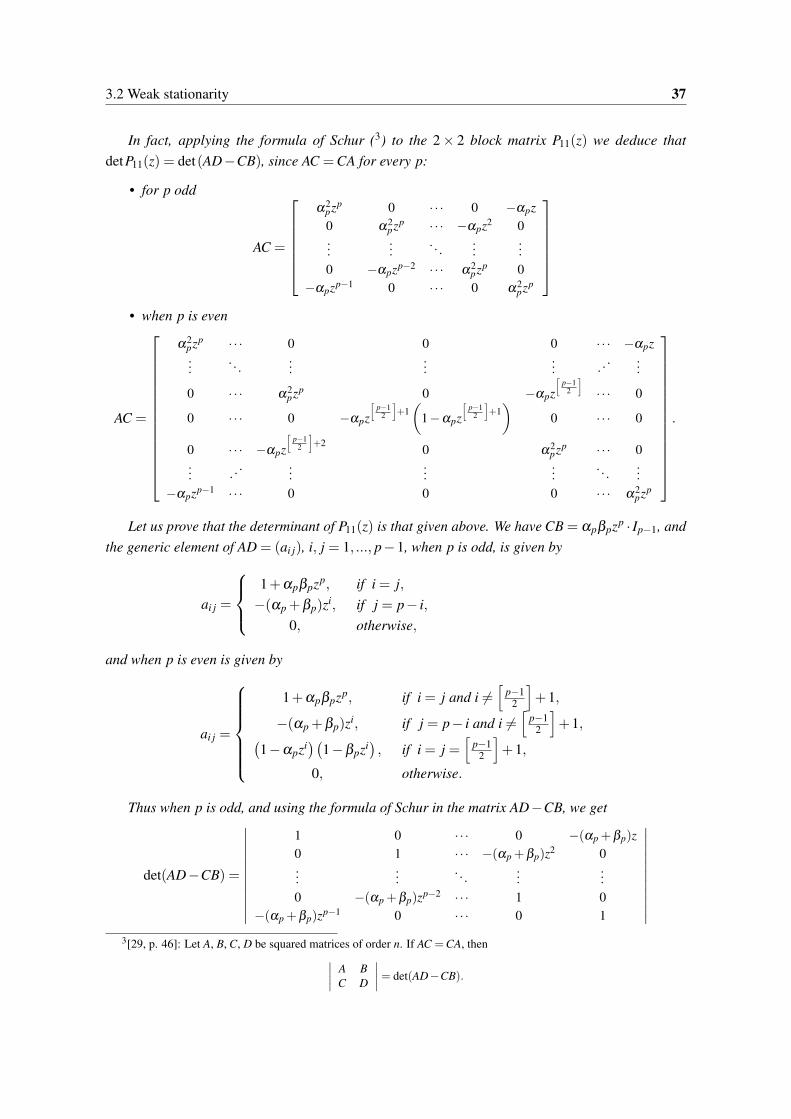
3.2 Weak stationarity 37
In fact, applying the formula of Schur (3) to the 2 × 2 block matrix P11(z) we deduce thatdetP11(z) = det(AD−CB), since AC =CA for every p:
• for p odd
AC =
α2
pzp 0 · · · 0 −αpz0 α2
pzp · · · −αpz2 0...
.... . .
......
0 −αpzp−2 · · · α2pzp 0
−αpzp−1 0 · · · 0 α2pzp
• when p is even
AC =
α2pzp · · · 0 0 0 · · · −αpz...
. . ....
......
......
0 · · · α2pzp 0 −αpz
[p−1
2
]· · · 0
0 · · · 0 −αpz[
p−12
]+1(
1−αpz[
p−12
]+1)
0 · · · 0
0 · · · −αpz[
p−12
]+2 0 α2
pzp · · · 0...
......
......
. . ....
−αpzp−1 · · · 0 0 0 · · · α2pzp
.
Let us prove that the determinant of P11(z) is that given above. We have CB = αpβpzp · Ip−1, andthe generic element of AD = (ai j), i, j = 1, ..., p−1, when p is odd, is given by
ai j =
1+αpβpzp, if i = j,−(αp +βp)zi, if j = p− i,
0, otherwise,
and when p is even is given by
ai j =
1+αpβpzp, if i = j and i =
[p−1
2
]+1,
−(αp +βp)zi, if j = p− i and i =[
p−12
]+1,(
1−αpzi)(
1−βpzi), if i = j =
[p−1
2
]+1,
0, otherwise.
Thus when p is odd, and using the formula of Schur in the matrix AD−CB, we get
det(AD−CB) =
∣∣∣∣∣∣∣∣∣∣∣
1 0 · · · 0 −(αp +βp)z0 1 · · · −(αp +βp)z2 0...
.... . .
......
0 −(αp +βp)zp−2 · · · 1 0−(αp +βp)zp−1 0 · · · 0 1
∣∣∣∣∣∣∣∣∣∣∣3[29, p. 46]: Let A, B, C, D be squared matrices of order n. If AC =CA, then∣∣∣∣ A B
C D
∣∣∣∣= det(AD−CB).

38 Stationarity and Ergodicity in the CP-INGARCH process
= det
I p−12−
(αp +βp)
2zp · · · 0...
. . ....
0 · · · (αp +βp)2zp
=
∣∣∣∣∣∣∣∣1− (αp +βp)
2zp · · · 0...
. . ....
0 · · · 1− (αp +βp)2zp
∣∣∣∣∣∣∣∣= [1− (αp +βp)2zp]
p−12 .
On the other hand, when p is even, applying the Laplace theorem to the ([ p−12 ]+1)-th row of the
matrix AD−CB we obtain that its determinant is given by∣∣∣∣∣∣∣∣∣∣∣∣∣∣∣∣
1 · · · 0 0 0 · · · −(αp +βp)z...
. . ....
......
......
0 · · · 1 0 −(αp +βp)z[p−1
2 ] · · · 0
0 · · · 0 1− (αp +βp)z[p−1
2 ]+1 0 · · · 0
0 · · · −(αp +βp)z[p−1
2 ]+2 0 1 · · · 0...
......
......
. . ....
−(αp +βp)zp−1 · · · 0 0 0 · · · 1
∣∣∣∣∣∣∣∣∣∣∣∣∣∣∣∣
= [1−(αp+βp)z[p−1
2 ]+1]
∣∣∣∣∣∣∣∣∣∣∣∣∣∣
1 · · · 0 0 · · · −(αp +βp)z...
. . ....
......
...
0 · · · 1 −(αp +βp)z[p−1
2 ] · · · 0
0 · · · −(αp +βp)z[p−1
2 ]+2 1 · · · 0...
......
.... . .
...−(αp +βp)zp−1 · · · 0 0 · · · 1
∣∣∣∣∣∣∣∣∣∣∣∣∣∣= [1− (αp +βp)z[
p−12 ]+1][1− (αp +βp)
2zp]p−2
2 ,
where the last equality follows using the same strategy as in the case of the p being odd.So, the necessary and sufficient condition for weak stationarity of the considered model is given by
(αp +βp)2 + v1α
2p < 1,
under αp+βp < 1, and plotted in Figure 3.1 considering different values of v1. We note that, contraryto what happens in the necessary and sufficient condition of first-order stationarity (Theorem 3.1), inthis case the condition is affected by the nature of the characteristic functions ϕt , via parameter v1.
Let us remember that the case v1 = 0 contains all the deterministic and independent of t characte-ristic functions ϕt . For instance, the dark to lightest gray region represented in Figure 3.1 corresponds,in particular, to the weak stationarity region for the INGARCH(1,1), GP-INGARCH(1,1), GEOMP2-INGARCH(1,1) and NTA-INGARCH(1,1) processes under the condition α1 +β1 < 1. We can alsoconclude, for example, that the weak stationarity region of the NTA-INGARCH(1,1) process, forany value of parameter φ (dark to lightest gray) is larger than the weak stationarity region of theGEOMP-INGARCH(1,1) process (recall in this case v1 = 2/r) considering r = 0.4 (darkest gray).These regions get closer when we increase the value of the parameter r.

3.2 Weak stationarity 39
Fig. 3.1 Weak stationarity regions of a CP-INGARCH(p, p) model under the condition αp +βp < 1,with the coefficients α1 = ... = αp−1 = β1 = ... = βp−1 = 0 and considering v1 = 5 (darkest gray),0.5 (darkest and medium gray) and 0 (dark to lightest gray).
Example 3.2 Let us consider a CP-INGARCH(2,2) model satisfying the hypothesis H2 and suchthat ∑
2j=1 (α j +β j)< 1. To examine the necessary and sufficient condition of weak stationarity we
consider the polynomial matrix P(z) = I3 −B1z−B2z2, with B1 and B2 the 3×3 matrices given by
B1 =
(α1 +β1)2 + v1α2
1 2(1+ v1)α2(α1 +β1) 2(1+ v1)β2(α1 +β1)
α1 +β1
1+v1α2 β2
α1+β11+v1
α2 β2
,
B2 =
(α2 +β2)2 + v1α2
2 0 00 0 00 0 0
.Thus the determinant of this polynomial is
detP(z) =(1− [(α1 +β1)
2 + v1α21 ]z− [(α2 +β2)
2 + v1α22 ]z
2)(1−α2z)(1−β2z)
−2(1+ v1)
(α1 +
β1
1+ v1
)α2β2(α1 +β1)z3 −2α2β2(α1 +β1)
2z3
−2(1+ v1)β2(α1 +β1)2(1−α2z)z2
−2(1+ v1)α2(α1 +β1)(1−β2z)(
α1 +β1
1+ v1
)z2
−α2β2(1− [(α1 +β1)
2 + v1α21 ]z− [(α2 +β2)
2 + v1α22 ]z
2)z2
= 1−[(α1 +β1)
2 +α2 +β2 + v1α21]
z
−[(α1 +β1)
2(α2 +β2)+(α2 +β2)2 + v1(α
22 −α
21 β2 +α
21 α2 +2α1α2β1)
]z2
−[−(α2 +β2)
3 − v1α22 (α2 +β2)
]z3.
Using, for instance, the Matlab software we can exhibit the roots of detP(z) in some particularcases. For example, if we consider α1 = α2 = β1, β2 = 0 and v1 = 0 we obtain the roots

40 Stationarity and Ergodicity in the CP-INGARCH process
z1 =− 1α1
, z2 =2α1 −2α2
1
(√1+α1
α31
+1)
α1, z3 =
2α1 +2α21
(√1+α1
α31
+1)
α1,
which are always outside the unit circle under the first-order stationarity condition 3α1 < 1. On theother hand, when we consider α1 = β1 = 0 we get the roots
z1 =1
α2 +β2, z2 =
1√(α2 +β2)2 + v1α2
2
, z3 =− 1√(α2 +β2)2 + v1α2
2
,
from where we deduce the condition (α2 +β2)2 + v1α2
2 < 1 already stated in Example 3.1.Taking β2 = 0, we plot in Figure 3.2 the weak stationarity regions of a CP-INGARCH(2,1) process
considering different values for v1, namely, v1 = 0, 0.5 and 5 (4).
Fig. 3.2 Weak stationarity regions of a CP-INGARCH(2,1) model with α1+α2+β1 < 1, consideringv1 = 0 (lightest gray), 0.5 (medium gray) and 5 (darkest gray).
Fig. 3.3 The three planes that define the weak stationarity regions of Figure 3.2.
We conclude that, as in Example 3.1, when we increase the value of v1 the weak stationarity regionbecomes smaller. To better view, we represent in Figure 3.3 the three planes that define the mentionedregions where it is now clear that the weak stationarity region with v1 = 5 (darkest gray) is containedin the weak stationarity region with v1 = 0.5 (darkest and medium gray) and this one is contained inthe weak stationarity region with v1 = 0 (dark to lightest gray). Let us note that the first plot of theFigure 3.3 corresponds to the CP-INARCH(2) weak stationarity regions.
In Appendix B we establish another necessary condition for weak stationarity which coincideswith the previous one in some particular cases, as we will prove.
4The program in MATLAB code can be found in Appendix D.2.

3.3 Moments structure 41
3.3 Moments structure
The autocorrelation function for the CP-INGARCH(p,q) model is derived in this section and il-lustrated when p = q = 1. Moreover, in this particular case, we deduce a necessary and sufficientcondition for the existence of unconditional moments of any order of the process.
3.3.1 The autocovariance function
We recall that in Theorem 3.2 we derive some values for the autocovariance function. Despite itssimplicity, especially when the orders p and q are low, these expressions are quite insufficient todescribe the autocovariance function. In fact, for example, for a CP-INGARCH(1,1) such expressionsallow us only to determine the value of V (Xt). In the next theorem we derive a set of equations fromwhich the autocovariance function of the general CP-INGARCH(p,q) model can be obtained.
Theorem 3.3 Let X be a weakly stationary CP-INGARCH(p,q) process. The autocovariances of theprocesses X and λ , respectively Γ and Γ, satisfy the linear equations
Γ(h) =p
∑j=1
α j ·Γ(h− j)+min(h−1,q)
∑k=1
βk ·Γ(h− k)+q
∑k=h
βk · Γ(k−h), h ≥ 1,
Γ(h) =min(h,p)
∑j=1
α j · Γ(h− j)+p
∑j=h+1
α j ·Γ( j−h)+q
∑k=1
βk · Γ(h− k), h ≥ 0,
assuming that ∑qk=h βk · Γ(k−h) = 0 if h > q and ∑
pj=h+1 α j ·Γ( j−h) = 0 if h ≥ p.
Proof: From expressions (3.3) and (3.4) we have
E (XtXt−h) = α0µ +p
∑j=1
α jE (Xt− jXt−h)+min(h−1,q)
∑k=1
βkE (Xt−kXt−h)+q
∑k=h
βkE (λt−kλt−h), h ≥ 1,
E (λtλt−h) = α0µ +min(h,p)
∑j=1
α jE (λt− jλt−h)+p
∑j=h+1
α jE (Xt− jXt−h)+q
∑k=1
βkE (λt−kλt−h), h ≥ 0.
Thus, for h ≥ 1, we obtain
Γ(h) = E[(Xt −µ)(Xt−h −µ)] = E (XtXt−h)−µ2
= α0µ +p
∑j=1
α j ·Γ(h− j)+min(h−1,q)
∑k=1
βk ·Γ(h− k)+q
∑k=h
βk · Γ(k−h)+µ2
(p
∑j=1
α j +q
∑k=1
βk
)−µ
2
=p
∑j=1
α j ·Γ(h− j)+min(h−1,q)
∑k=1
βk ·Γ(h− k)+q
∑k=h
βk · Γ(k−h),
and, for h ≥ 0, proceeding in an analogous way
Γ(k) = E[(λt −µ)(λt−h −µ)] = E(λtλt−h)−µ2

42 Stationarity and Ergodicity in the CP-INGARCH process
=min(h,p)
∑j=1
α j · Γ(h− j)+p
∑j=h+1
α j ·Γ( j−h)+q
∑k=1
βk · Γ(h− k),
which completes the proof.
We point out that this general result includes those of Weiß [77], Zhu [81, 82] and Xu et al. [80]on INGARCH, NB-INGARCH, GP-INGARCH and NB-DINARCH models as special cases.
The autocovariance function of the CP-INGARCH(p,q) process indicates that it can be representedas an ARMA process. In fact, as a consequence of Theorem 3.3 we have
Γ(h) =p
∑j=1
α j ·Γ(h− j)+min(h−1,q)
∑k=1
βk ·Γ(h− k)+q
∑k=h
βk · Γ(k−h), h ≥ 1,
=
p
∑j=1
α j ·Γ(h− j)+h−1
∑k=1
βk ·Γ(h− k)+q
∑k=h
βk · Γ(k−h), 1 ≤ h ≤ q,
p
∑j=1
α j ·Γ(h− j)+q
∑k=1
βk ·Γ(h− k), h ≥ q+1,
which means that Xt −µt∈Z has an ARMA(max(p,q),q) representation [12, p. 90]. We point outthat this result may be useful in the identification of the model, i.e., in the choice of the orders p and q.
For a CP-INGARCH(1,1) model we are able to present explicitly the autocovariance function.
Corollary 3.2 Let X be a weakly stationary CP-INGARCH(1,1) process.
The autocovariances of X are given by
Γ(h) =α1(1−β1(α1 +β1))(α1 +β1)
h−1
1− (α1 +β1)2 +α21
Γ(0), h ≥ 1.
Proof: From Theorem 3.3, we obtain for h ≥ 2 that
Γ(h) = α1 ·Γ(h−1)+β1 ·Γ(h−1) = (α1 +β1) ·Γ(h−1) = ...
= (α1 +β1)h−1 ·Γ(1) = (α1 +β1)
h−1[α1 ·Γ(0)+β1 · Γ(0)]. (3.12)
To determine an expression for V (λt) = Γ(0), we note first that for h ≥ 1,
Γ(h) = α1 · Γ(h−1)+β1 · Γ(h−1) = ... = (α1 +β1)h · Γ(0),
Γ(0) = α1 ·Γ(1)+β1 · Γ(1)
= α21 ·Γ(0)+α1β1 · Γ(0)+β1(α1 +β1) · Γ(0)
= α21 ·Γ(0)+ [(α1 +β1)
2 −α21 ] · Γ(0)
⇔ Γ(0) =α2
1 ·Γ(0)1− (α1 +β1)2 +α2
1.
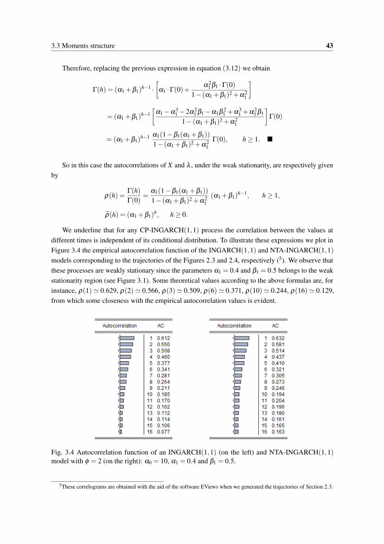
3.3 Moments structure 43
Therefore, replacing the previous expression in equation (3.12) we obtain
Γ(h) = (α1 +β1)h−1 ·
[α1 ·Γ(0)+
α21 β1 ·Γ(0)
1− (α1 +β1)2 +α21
]
= (α1 +β1)h−1[
α1 −α31 −2α2
1 β1 −α1β 21 +α3
1 +α21 β1
1− (α1 +β1)2 +α21
]Γ(0)
= (α1 +β1)h−1 α1(1−β1(α1 +β1))
1− (α1 +β1)2 +α21
Γ(0), h ≥ 1.
So in this case the autocorrelations of X and λ , under the weak stationarity, are respectively givenby
ρ(h) =Γ(h)Γ(0)
=α1(1−β1(α1 +β1))
1− (α1 +β1)2 +α21(α1 +β1)
h−1, h ≥ 1,
ρ(h) = (α1 +β1)h, h ≥ 0.
We underline that for any CP-INGARCH(1,1) process the correlation between the values atdifferent times is independent of its conditional distribution. To illustrate these expressions we plot inFigure 3.4 the empirical autocorrelation function of the INGARCH(1,1) and NTA-INGARCH(1,1)models corresponding to the trajectories of the Figures 2.3 and 2.4, respectively (5). We observe thatthese processes are weakly stationary since the parameters α1 = 0.4 and β1 = 0.5 belongs to the weakstationarity region (see Figure 3.1). Some theoretical values according to the above formulas are, forinstance, ρ(1)≃ 0.629, ρ(2)≃ 0.566, ρ(3)≃ 0.509, ρ(6)≃ 0.371, ρ(10)≃ 0.244, ρ(16)≃ 0.129,from which some closeness with the empirical autocorrelation values is evident.
Fig. 3.4 Autocorrelation function of an INGARCH(1,1) (on the left) and NTA-INGARCH(1,1)model with φ = 2 (on the right): α0 = 10, α1 = 0.4 and β1 = 0.5.
5These correlograms are obtained with the aid of the software EViews when we generated the trajectories of Section 2.3.

44 Stationarity and Ergodicity in the CP-INGARCH process
Remark 3.5 If the hypothesis H2 is satisfied then the variance of Xt is given by
Γ(0) = µ(v0 + v1µ)[1− (α1 +β1)
2 +α21 ]
1− (α1 +β1)2 − v1α21
,
where µ = α0/(1−α1 −β1). In fact, the variance of Xt can be obtained from
V (Xt) = E[(v0 + v1λt)λt ]+V (λt) = v0µ + v1E(λ 2t )+V (λt)
= v0µ +(1+ v1)V (λt)+ v1µ2
⇔ Γ(0) = v0µ +(1+ v1)α
21 ·Γ(0)
1− (α1 +β1)2 +α21+ v1µ
2
⇔[1− (α1 +β1)
2 − v1α21]
Γ(0) = µ(v0 + v1µ)[1− (α1 +β1)2 +α
21 ]
⇔ Γ(0) = µ(v0 + v1µ)[1− (α1 +β1)
2 +α21 ]
1− (α1 +β1)2 − v1α21
.
We observe that the variance Γ(0) can also be obtained by applying the formula stated in Theorem3.2 since, in this case, we have
P(1) = 1−B1 = 1− (α1 +β1)2 − v1α
21 ,
B0 = v0µ +(1+ v1)[2α0µ −α20 ]− v0µ(2α1β1 +β
21 ).
Therefore, if we consider α0 = 10, α1 = 0.4 and β1 = 0.5 then Γ(0) =35(v0 +100v1)
0.19−0.16v1.
In particular, for the INGARCH(1,1) process we get√
Γ(0)≃ 13.572 (v0 = 1 and v1 = 0), forthe NTA-INGARCH(1,1) process with φ = 2 we get
√Γ(0)≃ 23.508 (v0 = 1+φ and v1 = 0), and
for the GEOMP-INGARCH(1,1) process with r = 2 we get√
Γ(0)≃ 343.269 (v0 = 1 and v1 = 2/r).Comparing these theoretical values, respectively, with those presented in the simulated trajectoriesof Figures 2.3 (= 13.247), 2.4 (= 24.042) and 2.5 (= 133.902), we notice a discrepancy in theGEOMP-INGARCH which may be a consequence from its hight variability.
3.3.2 Moments of a CP-INGARCH(1,1)
In this section we give a necessary and sufficient condition for the existence of all moments of aCP-INGARCH(1,1). The study undertaken allows us to establish this result in a subclass of modelsfor which the characteristic functions ϕt satisfy
Hypothesis H3 : ϕt is deterministic.
We underline that this particular case still includes a wide class of models, many of them hereintroduced, as the GEOMP2-INGARCH or the NTA-INGARCH processes.
We start by presenting the next lemma which proof is in Appendix C.1.
3.3 Moments structure 45
Lemma 3.1 For k ∈ N0 and m ∈ N, the m-th derivative of the function ϕkt = ∏
kj=1 ϕt is given by
(ϕ
kt
)(m)(u) =
m−1
∑n=max0,m−k
k!(k−m+n)!
ϕk−m+nt (u) ×
∑k1+...+km=m−n
k1+2k2+...+mkm=mkr∈N0
(m;k1, ...,km)[ϕ′t (u)
]k1 ...[ϕ(m)t (u)]km , u ∈ R, (3.13)
where (m;k1, ...,km) represents the number of ways of partitioning a set of m = k1 +2k2 + . . .+mkm
different objects into kr subsets containing r objects for r = 1,2, . . . ,m, i.e., (see, e.g., [2, p. 823])
(m;k1, ...,km) =m!
(1!)k1k1!(2!)k2k2! . . .(m!)kmkm!.
Theorem 3.4 Let X be a CP-INGARCH(1,1) model such that the hypothesis H3 is satisfied. Themoments of X are all finite if and only if α1 +β1 < 1.
Proof: Let us recall the representation (2.5) stated in Section 2.3. Since the Xt, j, j = 1, ...,Nt , arei.i.d. random variables with common characteristic function ϕt , the characteristic function of the sum∑
kj=1 Xt, j is ∏
kj=1 ϕt(u) = ϕk
t (u), u ∈R. As Xt |X t−1 is a compound Poisson random variable, we have,according to Remark 2.3,
E[Xmt |X t−1] =
m
∑r=0
(λ ∗t )
r
r!
r
∑k=0
(rk
)(−1)r−kE
[(k
∑j=1
Xt, j
)m
|X t−1
]
=m
∑r=0
1r!
λ rt
(ϕ ′t (0))r
r
∑k=0
(rk
)(−1)r−k
im−r
(ϕ
kt
)(m)(0), m ≥ 1,
with(ϕk
t)(m) given by expression (3.13). Thus,
E[Xmt ] =
m
∑r=0
r
∑k=0
1r!
(rk
)(−1)r−k
(ϕk
t)(m)
(0)im−r(ϕ ′
t (0))r E[λ rt ]. (3.14)
The binomial formula yields
λrt = (α0 +α1Xt−1 +β1λt−1)
r =r
∑n=0
(rn
)α
r−n0
n
∑l=0
(nl
)α
l1β
n−l1 X l
t−1λn−lt−1
= αr0 +
r
∑n=1
(rn
)α
r−n0
[β
n1 λ
nt−1 +
n
∑l=1
(nl
)α
l1β
n−l1 X l
t−1λn−lt−1
].
As λn−lt−1 is X t−2-measurable we obtain
E[X lt−1λ
n−lt−1 |X t−2] =
l
∑v=0
1v!
λv+n−lt−1
(ϕ ′t−1(0))v
v
∑x=0
(vx
)(−1)v−x
il−v
(ϕ
xt−1)(l)
(0), l ≥ 1,

46 Stationarity and Ergodicity in the CP-INGARCH process
and consequently,
E[λ rt |X t−2] = α
r0 +
r
∑n=1
(rn
)α
r−n0
[β
n1 λ
nt−1 +
n
∑l=1
(nl
)α
l1β
n−l1 λ
n−lt−1 E[X l
t−1|X t−2]
]
= αr0 +
r
∑n=1
(rn
)α
r−n0 β
n1 λ
nt−1 +
r
∑n=1
(rn
)α
r−n0
n
∑l=1
(nl
)×
×l
∑v=0
α l1β
n−l1
v!(ϕ ′t−1(0))v
v
∑x=0
(vx
)(−1)v−x
il−v
(ϕ
xt−1)(l)
(0) λv+n−lt−1 . (3.15)
Let Λt = (λ mt , ...,λt)
⊤. In the algebraic expression of E[λ rt |X t−2], for r = 1, ...,m, all the powers
of λt−1 are less or equal to r. Therefore, a constant vector d and an upper triangular matrix D = (di j),i, j = 1, ...,m, exist such that the following equation is satisfied:
E[Λt |X t−2] = d+DΛt−1
⇔
E[λ m
t |X t−2]...
E[λ 2t |X t−2]
E[λt |X t−2]
=
αm
0...
α20
α0
+
(α1 +β1)m · · · ∗ ∗
.... . .
......
0 · · · (α1 +β1)2 ∗
0 · · · 0 α1 +β1
λ mt−1...
λ 2t−1
λt−1
.Indeed, let us prove that the diagonal entries of the matrix D are those given above.
The k-th diagonal entry of the matrix D corresponds to the case where in equation (3.15), weconsider r = m− k+1. Thus, to obtain the coefficient of λ
m−k+1t−1 , we look at the terms corresponding
to n = m− k+1 and l = v. Then, we get
dkk = βm−k+11 +
m−k+1
∑l=1
(m− k+1
l
)α l
1βm−k+1−l1
l!(ϕ ′t−1(0))l
l
∑x=0
(lx
)(−1)l−x (
ϕxt−1)(l)
(0)
= βm−k+11 +
m−k+1
∑l=1
(m− k+1
l
)α
l1β
m−k+1−l1
= (α1 +β1)m−k+1, k = 1, ...,m,
since it can be proved that
l
∑x=0
(lx
)(−1)l−x (
ϕxt−1)(l)
(0) = l! [ϕ ′t−1(0)]
l. (3.16)
In fact, using the expression (3.13) we obtain
l
∑x=0
(lx
)(−1)l−x (
ϕxt−1)(l)
(0) =l
∑x=0
(lx
)(−1)l−x
l−1
∑j=l−x
x!(x− l + j)!
ϕx−l+ jt−1 (0)
× ∑k1+...+kl=l− j
k1+2k2+...+lkl=lkr∈N0
(l;k1, ...,kl)[ϕ′t−1(0)
]k1 ... [ϕ(l)t−1(0)]
kl ,

3.3 Moments structure 47
and thus, for any arbitrarily fixed k1, ...,kl ∈N0 such that k1+ ...+kl = l− j and k1+2k2+ ...+ lkl = l,the coefficient of
[ϕ ′
t−1(0)]k1 . . . [ϕ
(l)t−1(0)]
kl is given by[l
∑x=0
(lx
)(−1)l−x x!
(x− (k1 + ...+ kl))!
](l;k1, ...,kl)
=
[l
∑x=k1+...+kl
(−1)l−x
(l − x)!(x− (k1 + ...+ kl))!
]l!(l;k1, ...,kl)
=(−1)l−(k1+...+kl)
(l − (k1 + ...+ kl))!
[l−(k1+...+kl)
∑m=0
(l − (k1 + ...+ kl)
m
)(−1)−m
]l!(l;k1, ...,kl).
When k1 = l, k2 = . . . = kl = 0, we obtain the coefficient l!(l; l,0, ...,0) = l!. Otherwise, thecoefficient equals zero. Therefore, we finally conclude the equality (3.16).
Since X t−3 ⊂ X t−2, we obtain
E[Λt |X t−3] = E [E(Λt |X t−2)|X t−3] = E[d+DΛt−1|X t−3]
= d+D E[Λt−1|X t−3] = d+D(d+DΛt−2) = d+Dd+D2Λt−2.
Iterating this recurrence l times gives:
E[Λt |X t−2−l] =(
Im +D+D2 + . . .+Dl)
d+Dl+1Λt−(l+1).
Substituting k = l +2 leads to:
E[Λt |X t−k] =
(k−2
∑r=0
Dr
)d+Dk−1
Λt−(k−1).
If the eigenvalues of D are inside the unit circle, i.e., if for any eigenvalue λ of D we have |λ |< 1then there is a norm ∥.∥ under Rm such that ∥D∥< 1 [51, Theorem 3.32] and then the matrix Im −D,where Im represents the identity matrix of order m, is invertible and we can write
k−2
∑r=0
Dr =∞
∑r=0
Dr −∞
∑r=0
Dr+k−1 =∞
∑r=0
Dr −Dk−1∞
∑r=0
Dr = (Im −D)−1(Im −Dk−1),
that is, we getE[Λt |X t−k] = (Im −D)−1(Im −Dk−1)d+Dk−1
Λt−(k−1).
So, we conclude that the eigenvalues of D (which coincide with its diagonal entries because it isan upper triangular matrix) are inside the unit circle if and only if α1 +β1 < 1. Consequently, sinceDk−1 → 0 when k → ∞, we have
limk→∞
E[Λt |X t−k] = (Im −D)−1d = E[Λt ],
and then from (3.14) all the moments of Xt of order ≤ m are finite.

48 Stationarity and Ergodicity in the CP-INGARCH process
As in the particular case studied by Ferland et al. [25] we assure the existence of all moments ofthis process under a very simple condition on the model coefficients. In accordance to these authors,we point out that it is an unexpected result taking into consideration what is known on the complexityanalysis and on the conditions of moments existence for conditional heteroscedastic models in general.
In the following we illustrate the expressions stated above in some particular cases.
Remark 3.6 Let us consider the
• INGARCH model:(ϕk)(m)
(u) = (ik)meiku and(ϕk)(m)
(0) = (ik)m, u ∈ R, m ≥ 1. Thus
E[Xmt ] =
m
∑r=0
r
∑k=0
1r!
(rk
)(−1)r−kkm E[λ r
t ] =m
∑r=0
S(m,r)E[λ rt ]. (6)
A complete proof for this particular case can be found in [25].• NTA-INGARCH model: We have
ϕk(u) = exp
(kφ(eiu −1
)),(
ϕk)(m)
(u) = imm
∑j=1
S(m, j)(kφ) j exp(kφ(eiu −1
)+ i ju
), u ∈ R. (3.17)
In fact, for m = 1, we get (ϕ
k(u))′
= ikφ exp(kφ(eiu −1
)+ iu
),
and, by induction,
(ϕ
k)(m+1)
(u) =ddu
[im
m
∑j=1
S(m, j)(kφ) j exp(kφ(eiu −1
)+ i ju
)]
= imm
∑j=1
S(m, j)(kφ) j (ikφeiu + i j)
exp(kφ(eiu −1
)+ i ju
)= im+1
m
∑j=1
S(m, j)[(kφ) j+1 exp
(kφ(eiu −1
)+ i( j+1)u
)+ j(kφ) j exp
(kφ(eiu −1
)+ i ju
)]= im+1
m
∑j=2
(kφ) j[S(m, j−1)+ jS(m, j)]exp(kφ(eiu −1
)+ i ju
)+im+1kφ exp
(kφ(eiu −1
)+ iu
)+im+1(kφ)m+1 exp
(kφ(eiu −1
)+ i(m+1)u
)= im+1
m+1
∑j=1
S(m+1, j)(kφ) j exp(kφ(eiu −1
)+ i ju
),
6[1, p. 835]: A closed form for the Stirling numbers of the second kind is
S(m,r) =1r!
r
∑k=0
(−1)r−k(
rk
)km.

3.4 Strict stationarity and Ergodicity 49
from the recurrence relation of the Stirling numbers of the second kind and so (3.17) is proved.
Taking u = 0, we conclude (ϕ
k)(m)
(0) = imm
∑j=1
S(m, j)(kφ) j.
Thus,
E[Xmt ] =
m
∑r=0
r
∑k=0
1r!
(rk
)(−1)r−k
φ r
m
∑j=1
S(m, j)(kφ) j E[λ rt ], (recall (3.14))
E[λ rt |X t−2] = α
r0 +
r
∑n=1
(rn
)α
r−n0 β
n1 λ
nt−1 +
r
∑n=1
(rn
)α
r−n0
n
∑l=1
(nl
)×
×l
∑v=0
α l1β
n−l1
v! φ v
l
∑k=1
v
∑j=0
(−1)v− jS(l,k)
(vj
)( jφ)k
λv+n−lt−1 , (recall (3.15))
and the diagonal entries of the matrix D are given by
dii =m−i+1
∑l=0
(m− i+1
l
)α l
1βm−i+1−l1l!φ l
l
∑k=1
l
∑j=0
(−1)l− jS(l,k)
(lj
)( jφ)k
=m−i+1
∑l=0
(m− i+1
l
)α
l1β
m−i+1−l1
l
∑k=1
S(l,k)S(k, l)φ k−l
= (α1 +β1)m−i+1, i = 1, ...,m,
because S(k, l) = 0 only when k = l.
3.4 Strict stationarity and Ergodicity
In this section we study the existence of strictly stationary solutions for the class of models previouslyintroduced. We begin by building, recursively, a first-order stationary process solution of the modelfollowing the theory presented by Ferland et al. [25]. This solution will be, under certain conditions,strictly stationary and ergodic.
Let us consider the CP-INGARCH model as specified in (2.2) and (2.3) associated to a givenfamily of characteristic functions (ϕt , t ∈ Z) such that H1 and H3 are satisfied and let ψ j j∈N0 bethe sequence of coefficients associated to the CP-INARCH(∞) representation of the model.
Let Utt∈Z be a sequence of independent real random variables distributed according to a discretecompound Poisson distribution with characteristic function
ΦUt (u) = exp
ψ0i
ϕ ′t (0)
[ϕt(u)−1].

50 Stationarity and Ergodicity in the CP-INGARCH process
For each t ∈ Z and k ∈ N, let Zt,k = Zt,k, j j∈N be a sequence of independent discrete compoundPoisson random variables with characteristic function
ΦZt,k, j(u) = exp
ψki
ϕ ′t+k(0)
[ϕt+k(u)−1].
We note that E(Ut)=ψ0, E(Zt,k, j)=ψk and that Zt,k, j are identically distributed for each (t,k)∈Z×N.We also assume that all the variables Us, Zt,k, j, (s, t ∈ Z and k, j ∈ N), are mutually independent.
Based on these random variables, we define the sequence X (n)t as follows:
X (n)t =
0, n < 0Ut , n = 0
Ut +n
∑k=1
X (n−k)t−k
∑j=1
Zt−k,k, j, n > 0
(3.18)
where it is assumed that ∑0j=1 Zt−k,k, j = 0. Using the notion of thinning operation (7), X (n)
t admits, forn > 0, the representation
X (n)t =Ut +
n
∑k=1
ψ(t−k)k X (n−k)
t−k , (3.19)
where the notation (ψ(τ)k ) means that the sequence of random variables of mean ψk involved in the
thinning operation corresponds to time τ , i.e., the sequence Zτ,k = Zτ,k, j j∈N. Note that we canreally use the thinning operation since Zt−k,k is a sequence of i.i.d. random variables and X (n−k)
t−k andZt−k,k, j are independent, for each k ∈ 1, ...,n. Indeed, for a fixed k, we have
X (n−k)t−k =Ut−k +
n−k
∑r=1
X (n−k−r)t−k−r
∑j=1
Zt−k−r,r, j
= fn
(Ut−k, X (n−k−1)
t−k−1 , X (n−k−2)t−k−2 , . . . , X (1)
t−n+1, Ut−n, Zt−k−1,1, j, . . . , Zt−n+1,n−k−1, j, Zt−n,n−k, j, j ∈ N)
= fn
(Ut−k, Ut−k−1, X (n−k−2)
t−k−2 , . . . , X (1)t−n+1, Ut−n, Zt−k−1,1, j, Zt−k−2,2, j, . . . , Zt−n+1,n−k−1, j,
Zt−n,n−k, j, Zt−k−2,1, j, Zt−k−3,2, j, . . . , Zt−n+1,n−k−2, j, Zt−n,n−k−1, j, j ∈ N)
= . . . = fn(Ut−k, . . . , Ut−n, Zt−k−r,s, j, r = 1, ...,n− k, s = 1, ...,r, j ∈ N
),
and the required independence holds from the construction of the variables.
The representation (3.19) shows that X (n)t is obtained through a cascade of thinning operations
along the sequence Utt∈Z. Indeed, using recursively the thinning operator, we have
7[30]: Let X be a nonnegative integer-valued random variable. For any α ≥ 0 the thinning operation is defined by
α X =
∑
Xj=1 Y j, if X > 0,
0, otherwise,
where ’’ denotes the thinning operator, Y j is a sequence of i.i.d. nonnegative integer-valued random variables, independentof X , and such that E(Y j) = α . The sequence Y j is known as counting series. In the binomial thinning operation thecounting series is considered to be a sequence of i.i.d. Bernoulli random variables with parameter α .

3.4 Strict stationarity and Ergodicity 51
X (1)t = Ut +ψ
(t−1)1 X (0)
t−1 =Ut +ψ(t−1)1 Ut−1,
X (2)t = Ut +ψ
(t−1)1 X (1)
t−1 +ψ(t−2)2 X (0)
t−2
= Ut +ψ(t−1)1
(Ut−1 +ψ
(t−2)1 Ut−2
)+ψ
(t−2)2 Ut−2,
X (3)t = Ut +ψ
(t−1)1
[Ut−1 +ψ
(t−3)2 Ut−3 +ψ
(t−2)1
(Ut−2 +ψ
(t−3)1 Ut−3
)]+ψ
(t−2)2
(Ut−2 +ψ
(t−3)1 Ut−3
)+ψ
(t−3)3 Ut−3,
and so on. For any value n, X (n)t can be expanded in that way, which is useful on the study of its strict
stationarity and ergodicity.In what follows we present some properties of the sequence X (n)
t n∈N, useful on the analysisof its probabilistic behavior. In fact, we will prove that (X (n)
t , t ∈ Z), n ∈ Z is a non-decreasingsequence of first-order stationary processes that converges almost surely, in L1 and in L2.
Theorem 3.5 If ∑pj=1 α j +∑
qk=1 βk < 1 then (X (n)
t , t ∈ Z), n ∈ Z is a sequence of first-order
stationary processes such that µn = E(X (n)t )−→ µ , as n → ∞.
Proof: We start by noting that the expectation of X (n)t is well defined because X (n)
t is a finite sumof independent compound Poisson random variables. We will denote this expectation by µn and weprove in the following by induction, with respect to n ∈ Z, that it does not depend on t.
For n = 0 we obtain E(X (0)t ) = E(Ut) = ψ0, which is independent of t (for n < 0 the result is
trivial). Now let us consider as induction hypothesis, that for n > 0 and for any fixed value of t,E(X (n)
t ) is independent of t. Thus, from the mean of the thinning random variable (8.), we obtain
E(
X (n+1)t
)= E
(Ut +
n+1
∑k=1
ψ(t−k)k X (n+1−k)
t−k
)= ψ0 +
n+1
∑k=1
ψkE(
X (n+1−k)t−k
)
= g(
E(
X (0)t−n−1
), ...,E
(X (n)
t−1
)),
which is, by the induction hypothesis, a function independent of t. So
µn = E(
X (n)t
)=
0, n < 0ψ0, n = 0
ψ0 +n
∑k=1
ψkµn−k, n > 0,
and using the fact that µn−k = 0 if k > n, we can write
µn =∞
∑k=1
ψkµn−k +ψ0 = B−1(L) [A(L)µn +α0] ⇔ B(L)µn = A(L)µn +α0
⇔ K(L)µn = α0,
8[30, p. 52]: E [α X ] = αE [X ].More properties of the thinning operation can be found in [30] and [71]

52 Stationarity and Ergodicity in the CP-INGARCH process
where K(L) = B(L)−A(L) with A(L) and B(L) the polynomials introduced in Section 2.2.The last equation indicates that the sequence µnn∈Z satisfies a finite difference equation of degree
max(p,q) with constant coefficients, namely the equation µn −∑pj=1 α jµn− j −∑
qk=1 βkµn−k = α0.
The characteristic polynomial of this equation, K(z), has all its roots outside the unit circle since∑
pj=1 α j +∑
qk=1 βk < 1 and so, (X (n)
t , t ∈ Z), n ∈ Z is a sequence of first-order stationary processes.From this stationarity, we deduce that µn = ψ0 +∑
nk=1 ψkµn, n > 0, and then
limn→∞
µn =ψ0
1−∑∞k=1 ψk
=α0B−1(1)
1−A(1)B−1(1)=
α0
K(1)=
α0
1−∑pj=1 α j −∑
qk=1 βk
= µ.
Theorem 3.6 For a fixed value of t, the sequence (X (n)t , t ∈Z), n∈Z is a non-decreasing sequence
of nonnegative integer-valued random variables.
Proof: This result is stated by induction with respect to n, for any fixed value of t. In fact, we have
X (1)t −X (0)
t =Ut +
X (0)t−1
∑j=1
Zt−1,1, j −Ut =Ut−1
∑j=1
Zt−1,1, j,
which is nonnegative because this is a random sum of nonnegative integer-valued random variables.Let us suppose now that, for n > 0, X (n+1)
t −X (n)t ≥ 0. So,
X (n+2)t −X (n+1)
t =Ut +n+2
∑k=1
X (n+2−k)t−k
∑j=1
Zt−k,k, j −Ut −n+1
∑k=1
X (n+1−k)t−k
∑j=1
Zt−k,k, j
=
X (n+1)t−1
∑j=1
Zt−1,1, j +
X (n)t−2
∑j=1
Zt−2,2, j + . . . +
X (1)t−n−1
∑j=1
Zt−n−1,n+1, j +Ut−n−2
∑j=1
Zt−n−2,n+2, j
−X (n)
t−1
∑j=1
Zt−1,1, j −X (n−1)
t−2
∑j=1
Zt−2,2, j − . . . −X (0)
t−n−1
∑j=1
Zt−n−1,n+1, j.
By the induction hypothesis it follows that X (n+1)t−1 ≥ X (n)
t−1, X (n)t−2 ≥ X (n−1)
t−2 , ..., X (1)t−n−1 ≥ X (0)
t−n−1.Using that, we can rewrite the above equality in the form
X (n+2)t −X (n+1)
t =
X (n+1)t−1
∑j=X (n)
t−1+1
Zt−1,1, j + . . . +
X (1)t−n−1
∑j=X (0)
t−n−1+1
Zt−n−1,n+1, j +Ut−n−2
∑j=1
Zt−n−2,n+2, j
=n+1
∑k=1
X (n+2−k)t−k
∑j=X (n+1−k)
t−k +1
Zt−k,k, j +Ut−n−2
∑j=1
Zt−n−2,n+2, j,
which is once again a nonnegative integer-valued random variable.Then, (X (n)
t , t ∈ Z),n ∈ Z is, for each t, a non-decreasing sequence.
3.4 Strict stationarity and Ergodicity 53
Theorem 3.7 If ∑pj=1 α j +∑
qk=1 βk < 1 then the sequence (X (n)
t , t ∈ Z), n ∈ Z converges almostsurely and in L1 (or in mean) to a process X∗ = (X∗
t , t ∈ Z).
Proof: Let (Ω,A ,P) be the common probability space on which the relevant random variables aredefined. Since X (n)
t is a non-decreasing sequence of nonnegative integers we have
∀ ω ∈ Ω, limn→∞
X (n)t (ω) = X∗
t (ω),
where the limit X∗t (ω) is not necessarily finite. To prove the almost sure convergence of this sequence
we will use the Borel-Cantelli Lemma (9). In fact, we need to prove that X∗t (ω) is finite with
probability one which is equivalent to say that the set A∞ = ω : X∗t (ω) = ∞ is of probability zero,
i.e., P(A∞) = 0. But it is equivalent to prove that the events
An =
ω : X (n)t (ω)−X (n−1)
t (ω)> 0
occur infinitely often with probability zero, i.e., P(limsupn An) = 0.In fact, we have
E[X (n)
t −X (n−1)t
]=
+∞
∑k=1
kP(
ω : X (n)t (ω)−X (n−1)
t (ω) = k)
≥+∞
∑k=1
P(
ω : X (n)t (ω)−X (n−1)
t (ω) = k)
= P(An). (3.20)
On the other hand
E[X (n)
t −X (n−1)t
]= µn −µn−1 = ψ0 +
n
∑k=1
ψkµn−k −ψ0 −n−1
∑k=1
ψkµn−1−k = νn
⇔ ψnµ0 +n−1
∑k=1
ψk (µn−k −µn−k−1) = νn ⇔ νn =n
∑k=1
ψkνn−k.
Since νn−k = 0 if k > n, we conclude
νn =∞
∑k=1
ψkνn−k ⇔ νn = B−1(L)A(L)νn ⇔ K(L)νn = 0, (3.21)
where, as in the proof of Theorem 3.5, K(L) = B(L)−A(L). So, the sequence νnn∈N satisfies ahomogeneous finite difference equation with characteristic polynomial K(z) that has all roots outsidethe unit circle because ∑
pj=1 α j +∑
qk=1 βk < 1. From Section 3.6 of [12], we know that the general
solution of the equation (3.21) has the form
νn =k
∑j=1
r j−1
∑s=0
c jsnsξ−nj ,
where ξ j, j = 1, ...,k are the distinct roots of K(z), r j is the multiplicity of the root ξ j and c js a setof coefficients determined by the initial conditions. Thus, the sequence νnn∈N tends towards zero
9[65, p. 102]: Let An be any events. If ∑n P(An)< ∞ then P(limsupn→∞ An) = 0.

54 Stationarity and Ergodicity in the CP-INGARCH process
with a geometric rate as n → ∞. In other words, there exist constants M ≥ 0 and 0 < c < 1 such thatνn ≤ Mcn. Using (3.20) and (3.21) we get P(An)≤ νn and then
∞
∑n=1
P(An)≤ M∞
∑n=1
cn < ∞.
Finally, from the Borel-Cantelli lemma, we obtain P(limsupn An) = 0, which allow us to concludethe almost sure convergence of the sequence (X (n)
t , t ∈ Z),n ∈ Z to a process X∗t t∈Z.
For the L1 convergence, recall that we have nonnegative integer-valued random variables. ApplyingBeppo Lévi’s Theorem and then Theorem 3.5 we conclude that the first moment of X∗
t t∈Z is finite,namely E(X∗
t ) = limn→∞ E(X (n)t ) = limn→∞ µn = µ . Consequently limn→∞ E(|X (n)
t −X∗t |) = 0.
Theorem 3.8 If ∑pj=1 α j +∑
qk=1 βk < 1 and (ϕt , t ∈ Z) is derivable at zero up to order 2 then the
sequence (X (n)t , t ∈ Z), n ∈ Z converges in L2 (or in quadratic mean) to the process X∗
t t∈Z.
Proof: To prove the convergence in L2 we start by showing that the second moment of X∗t is finite.
In fact, for n > 0, we obtain
E[(
X (n)t
)2]= E
Ut +
n
∑k=1
X (n−k)t−k
∑j=1
Zt−k,k, j
2
= E[U2t ]+2E
Ut
n
∑k=1
X (n−k)t−k
∑j=1
Zt−k,k, j
+E
n
∑k=1
X (n−k)t−k
∑j=1
Zt−k,k, j
2 (3.22)
By construction, Us and Zt,k, j (s, t ∈ Z and k, j ∈ N) are mutually independent and so
E
Ut
n
∑k=1
X (n−k)t−k
∑j=1
Zt−k,k, j
= E (Ut)E
n
∑k=1
X (n−k)t−k
∑j=1
Zt−k,k, j
= ψ0
n
∑k=1
ψkE(
X (n−k)t
)≤ ψ0E (X∗
t )n
∑k=1
ψk,
using the first-order stationarity of the process X (n)t and the fact that E(X (n)
t )≤ E(X∗t ) since X (n)
t is anon-decreasing sequence in n that converges almost surely to X∗
t . We have also
E
n
∑k=1
X (n−k)t−k
∑j=1
Zt−k,k, j
2=∞
∑x=0
E
n
∑k=1
X (n−k)t−k
∑j=1
Zt−k,k, j
2
| X (n−k)t−k = x
P(
X (n−k)t−k = x
)
=∞
∑x=0
V
(n
∑k=1
x
∑j=1
Zt−k,k, j
)+
(E
[n
∑k=1
x
∑j=1
Zt−k,k, j
])2P(
X (n−k)t−k = x
)
= E(
X (n−k)t−k
) n
∑k=1
V(Zt−k,k, j
)+E
[(X (n−k)
t−k
)2]( n
∑k=1
ψk
)2
(3.23)
3.4 Strict stationarity and Ergodicity 55
≤ E(
X (n)t
) n
∑k=1
V(Zt−k,k, j
)+E
[(X (n)
t
)2]( n
∑k=1
ψk
)2
,
where to obtain the equality (3.23) we use the independence of the random variables Zt,k, j (t ∈ Z andk, j ∈ N) and the fact that E[∑n
k=1 ∑xj=1 Zt−k,k, j] = ∑
nk=1 ∑
xj=1 E[Zt−k,k, j] = x∑
nk=1 ψk.
Using the hypothesis H3 and the relation between the characteristic function of Zt−k,k, j and itsmoments we get
V(Zt−k,k, j
)=−Φ
′′Zt−k,k, j
(0)−ψ2k =−i
ϕ ′′t (0)
ϕ ′t (0)
ψk = Rt(ψk)< ∞,
since
Φ′Zt−k,k, j
(u) = iψkϕ ′
t (u)ϕ ′
t (0)exp
ψki
ϕ ′t (0)
[ϕt(u)−1],
Φ′′Zt−k,k, j
(u) =
[iψk
ϕ ′′t (u)
ϕ ′t (0)
+
(iψk
ϕ ′t (u)
ϕ ′t (0)
)2]
exp
ψki
ϕ ′t (0)
[ϕt(u)−1].
So, we obtain
E
n
∑k=1
X (n−k)t−k
∑j=1
Zt−k,k, j
2≤n
∑k=1
Rt(ψk)E(
X (n)t
)+
(n
∑k=1
ψk
)2
E[(
X (n)t
)2]
≤n
∑k=1
Rt(ψk)E (X∗t )+
(n
∑k=1
ψk
)2
E[(
X (n)t
)2],
and finally replacing in (3.22) we obtain
E[(
X (n)t
)2]≤ E(U2
t )+2ψ0E (X∗t )
n
∑k=1
ψk +n
∑k=1
Rt(ψk)E (X∗t )+
(n
∑k=1
ψk
)2
E[(
X (n)t
)2].
Hence,
E[(
X (n)t
)2]≤ E(X∗
t )(∑nk=1 Rt(ψk)+2ψ0 ∑
nk=1 ψk)+E(U2
t )
1− (∑nk=1 ψk)
2
≤ E(X∗t )(∑
∞k=1 Rt(ψk)+2ψ0 ∑
∞k=1 ψk)+E(U2
t )
1− (∑∞k=1 ψk)
2 =Ct ,
with Ct a constant dependent of t. By Lebesgue’s dominated convergence theorem (10), we concludethat E[(X∗
t )2] is finite. Since the first two moments of X (n)
t n∈N are finite consequently the randomvariables X (n)
t are in L2(Ω,A ,P). Let us define V (n)t = (X (n)
t −X∗t )
2. The sequence V (n)t n∈N is
decreasing, bounded below by 0 and it satisfies E(V (0)t ) = E[(Ut −X∗
t )2]< ∞. Consequently,
limn→∞
E[(X (n)t −X∗
t )2] = lim
n→∞E[V (n)
t
]= E
[limn→∞
(a.s.)V (n)t
]= 0,
10[65, p. 133]: Let Xnn∈N be a sequence of random variables which converges a.s. or in probability to a randomvariable X . If there exists a random variable Y ∈ L1 such that |Xn| ≤ Y , then limn→∞ E(Xn) = E(X).
56 Stationarity and Ergodicity in the CP-INGARCH process
by Lebesgue’s dominated convergence theorem because X (n)t n∈N converges almost surely to X∗
t .Hence, we deduce that X (n)
t n∈N also converges to X∗t in L2(Ω,A ,P).
We have defined a sequence that has an almost sure and a mean-squared limit, but we still have toverify that this is a solution of the CP-INGARCH model. This is the goal of the next theorem.
Theorem 3.9 Under the hypothesis H3, if ∑pj=1 α j +∑
qk=1 βk < 1 the process X∗ is a first-order
stationary solution of the CP-INGARCH(p,q) model.
Proof: We shall prove the theorem in two steps. First we prove that, for all t ∈ Z, the characte-ristic function of X∗
t conditioned on X∗t−1, denoted by ΦX∗
t |X∗t−1
, is equal to limn→+∞ Φn with Φn the
characteristic function of the sequence r(n)t |X∗t−1n∈N, where
r(n)t =Ut +n
∑k=1
X∗t−k
∑j=1
Zt−k,k, j.
This equality follows from the Lévy Continuity Theorem since, for a fixed t, r(n)t |X∗t−1n∈N
converges in law to X∗t |X∗
t−1. Indeed, let us denote by Y (n)t the sequence r(n)t −X (n)
t . Then
Y (n)t =Ut +
n
∑k=1
X∗t−k
∑j=1
Zt−k,k, j −Ut −n
∑k=1
X (n−k)t−k
∑j=1
Zt−k,k, j =n
∑k=1
X∗t−k
∑j=X (n−k)
t−k +1
Zt−k,k, j ≥ 0,
because X (n−k)t−k n∈N is a non-decreasing sequence that converges almost surely to X∗
t−k. Additionally,
E[Y (n)
t
]= E
n
∑k=1
X∗t−k
∑j=X (n−k)
t−k +1
Zt−k,k, j
=n
∑k=1
E
X∗t−k
∑j=X (n−k)
t−k +1
Zt−k,k, j
=n
∑k=1
[∞
∑x=0
x E(Zt−k,k, j
)P(
X∗t−k −X (n−k)
t−k = x)]
=n
∑k=1
ψk E[X∗
t−k −X (n−k)t−k
]= µ
n
∑k=1
ψk −n
∑k=1
ψk µn−k,
which allows us to conclude
limn→∞
E[Y (n)
t
]= lim
n→∞
(µ
n
∑k=1
ψk −n
∑k=1
ψk µn−k
)= µ H(1)− lim
n→∞
n
∑k=1
ψk µn−k
=α0 A(1)
B(1) [B(1)−A(1)]− lim
n→∞
(µn +
α0
B(1)
), from Theorem 3.5,
=α0A(1)
B(1) [B(1)−A(1)]− α0
B(1)−A(1)+
α0
B(1)= 0.
This means that, when n → ∞, the sequence Y (n)t n∈N converges to zero in L1 because Y (n)
t isnonnegative. So, from the relation between the different types of convergence, Y (n)
t n∈N also
3.4 Strict stationarity and Ergodicity 57
converges in probability to zero and the same happens to X∗t −X (n)
t . Therefore,
X∗t − r(n)t = (X∗
t −X (n)t )+(X (n)
t − r(n)t ) = (X∗t −X (n)
t )−Y (n)t ,
allows us to conclude that r(n)t n∈N converges in probability to X∗t and then r(n)t |X∗
t−1n∈N convergesin law to X∗
t |X∗t−1. From that, we deduce finally ΦX∗
t |X∗t−1(u) = limn→+∞ Φn(u), u ∈ R.
The second step reduces to the calculation of Φn and then realize that Φn(u), u ∈ R, equalsexpi λt
ϕ ′(0) [ϕ(u)−1], when n → ∞. So, let us obtain Φn. Conditionally to X∗t−1, we have
Φ∑
X∗t−k
j=1 Zt−k,k, j(u) =
X∗t−k
∏j=1
ΦZt−k,k, j(u) = exp
X∗
t−k
∑j=1
ψki
ϕ ′t (0)
[ϕt(u)−1]
= exp
ψk X∗t−k
iϕ ′
t (0)[ϕt(u)−1]
, u ∈ R.
From the independence of the variables involved in the definition of r(n)t , we get
Φn(u) = exp
(ψ0
iϕ ′
t (0)[ϕt(u)−1]+
n
∑k=1
ψk X∗t−k
iϕ ′
t (0)[ϕt(u)−1]
)
= exp
(ψ0 +
n
∑k=1
ψk X∗t−k
)i
ϕ ′t (0)
[ϕt(u)−1]
, u ∈ R,
and thus, we have
limn→+∞
Φn(u) = exp
iλt
ϕ ′t (0)
[ϕt(u)−1], u ∈ R.
These two steps together enable us to conclude that the almost sure limit of the sequence X (n)t n∈N
is a solution of the model. The first-order stationarity of this solution is a consequence of Theorem3.1. We observe that from the unicity of the limit follows that this solution is uniquely defined.
Remark 3.7 From Theorems 3.7 and 3.8, we conclude that the condition ∑pj=1 α j +∑
qk=1 βk < 1
guarantees the existence of a second-order solution of a CP-INGARCH(p,q) process.
Now let us consider, additionally to the hypothesis H3, that ϕt is independent of t, i.e.,
Hypothesis H4 : ϕt = ϕ and ϕ deterministic.
In this subclass, which still includes, among others, the INGARCH, the NB-DINARCH, theNTA-INGARCH and the GEOMP2-INGARCH models, it is possible to set the strict stationarity andthe ergodicity of X (n)
t n∈N and the same for the process X∗t t∈Z.
Theorem 3.10 Under the hypothesis H4, (X (n)t , t ∈ Z), n ∈ Z is a sequence of strictly stationary
and ergodic processes.

58 Stationarity and Ergodicity in the CP-INGARCH process
Proof: Let us start by proving the strict stationarity. To simplify the notation we will prove thestatement only for a two-dimensional random vector, i.e., for any positive integer h we show that
X(n)12 = (X (n)
1 ,X (n)2 )⊤ and X(n)
1+h,2+h = (X (n)1+h,X
(n)2+h)
⊤
have the same joint distribution when n > 0. As the probability generating function characterizes thedistribution, let us prove that the probability generating functions of these random vectors (11) are thesame. Since X (n)
1 = f (U1−n, ...,U1) and X (n)2 = f ∗ (U2−n, ...,U2),
gX(n)12(s) = E
[sX (n)
11 sX (n)
22
]= E
(E[
sX (n)1
1 sX (n)2
2 |U1−n...2
])
= ∑x∈N2+n
E[
sX (n)1
1 sX (n)2
2 |U1−n...2 = x]
P(U1−n...2 = x),
where U1−n...2 represents the vector (U1−n, ...,U2)⊤. For a given value ut−n...t+1 = (ut−n, ...,ut+1)
⊤ ofthe random vector Ut−n...t+1, the components of the vector (X (n)
t ,X (n)t+1)
⊤ are computed using a set ofwell-determined variables coming from the sequences Zτ,η , τ = t −n, ..., t and η = 1, ...,n. It followsthat if U1−n...2 and U1−n+h...2+h are fixed to the same value x, the conditional distributions of X(n)
12 andX(n)
1+h,2+h given U1−n...2 and U1−n+h...2+h, respectively, are the same and hence
E[
sX (n)
1+h1 s
X (n)2+h
2 |U1−n+h...2+h = x]= E
[sX (n)
11 sX (n)
22 |U1−n...2 = x
].
As under the hypothesis H4 the vectors U1−n...2 and U1−n+h...2+h are of components identicallydistributed we have P(U1−n+h...2+h = x) = P(U1−n...2 = x), and so
gX(n)12(s) = ∑
x∈N2+n
E[
sX (n)
1+h1 s
X (n)2+h
k |U1−n+h...2+h = x]
P(U1−n+h...2+h = x) = gX(n)1+h,2+h
(s),
which allows to conclude that X(n)12 and X(n)
1+h,2+h have the same joint distribution for any h ∈ Z.
Analogously, it can be proved that for any k,h ∈ Z the random vectors X(n)1...k and X(n)
1+h...k+h, have the
same joint distribution and then the strict stationarity of the process X (n)t t∈Z, for each n, is deduced.
Regarding the ergodicity, under H4, the sequences (Ut , t ∈ Z) and (Zt,k, t ∈ Z,k ∈ N) previouslyintroduced are of i.i.d. random variables. Then, (X (n)
t , t ∈ Z), n ∈ Z is a sequence of ergodic pro-cesses, because it is a measurable function of the sequence of i.i.d. random variables (Ut ,Zt, j), t ∈Z,j ∈ N, say X (n)
t = Tn (Ut , . . . ,Ut−n,Zt−r,s,k, r = 1, . . . ,n, s = 1, . . . ,r, k ∈ N) (12).
11Let W be a random vector with nonnegative integer-valued entries and let p(W) denotes P(W = (w1, . . . ,wk)⊤). The
probability generating function of W, for s = (s1, . . . ,sk)⊤ ∈ [−1,1]k, is given by
gW(s) = E[sW11 . . .sWk
k ] = ∑w∈Nk
p(W)k
∏j=1
sw jj .
12[7, p. 32]: A sequence X of i.i.d. random variables is an ergodic process.[68, p. 33]: Let g : RZ → R be a measurable function and X be an ergodic process. Then the process Y = (Yt , t ∈ Z) with
Yt = g(...,Xt−1,Xt ,Xt+1, ...) is also ergodic.

3.4 Strict stationarity and Ergodicity 59
Theorem 3.11 Let us consider the model CP-INGARCH(p,q) such that H4 is satisfied.There is a strictly stationary and ergodic process that satisfies the model if ∑
pj=1 α j +∑
qk=1 βk < 1.
Moreover, the first two moments of this process are finite.
Proof: In Theorem 3.9 we proved that X∗t t∈Z is a solution of the CP-INGARCH model. So, it is
enough to prove that under the hypothesis H4, the process X∗t t∈Z is strictly stationary and ergodic.
Let us start with the strict stationarity. From Theorem 3.10, X (n)t n∈N is a sequence of strictly
stationary processes. Otherwise, X (n)t n∈N converges almost surely to X∗
t when ∑pj=1 α j+∑
qk=1 βk < 1.
So, considering without loss of generality, the indexes 1, ...,k, we have, for any h ∈ Z, the followingalmost sure convergence
(X (n)1 , ...,X (n)
k )a.s.−→n→+∞ (X∗
1 , ...,X∗k ),
(X (n)1+h, ...,X
(n)k+h)
a.s.−→n→+∞ (X∗1+h, ...,X
∗k+h),
and consequently, also the convergence in law. Considering the strict stationarity of X (n)t n∈N and
the unicity of the limit, we conclude that X∗t t∈Z is a strictly stationary process.
To prove the ergodicity, we note that X∗t t∈Z may be written as X∗
t = T ((Ut ,Zt, j), t ∈ Z, j ∈ N)where T is the almost sure limit of the sequence of the measurable functions Tn. T is then a measurablefunction, and so the process X∗
t t∈Z is ergodic as it is a measurable function of an ergodic process.The existence of the two first moments of X∗
t t∈Z is ensured by Theorems 3.7 and 3.8.
Remark 3.8 (a) Under the conditions of the previous theorem it follows that X∗t t∈Z is also a
weakly stationary solution of the model because it is a strictly stationary second-order process.
(b) In the set of the L1 processes, the condition of the previous theorem is necessary and sufficient forthe existence of a strictly stationary and ergodic process solution of the CP-INGARCH(p,q).
We finish the section by stating that, to the best of our knowledge, the general technique hereproposed to show the ergodicity is different from those existing in the literature for the integer-valuedmodels [13, 16, 52, 56] since we established the ergodicity of the strict stationarity solution displayed.


Chapter 4
CP-INARCH(1) process: Moments andEstimation Procedure
The CP-INARCH(1) process has a simple structure and a great potential for applications in practice.This simple model with its AR(1)-like serial dependence structure has already proved to be of greatpractical relevance, with particular applications namely in monthly claims counts of workers in theheavy manufacturing industry ([77]), daily download counts of the program CW β TeXpert ([85]),monthly strike data published by the U.S. Bureau of Labor Statistics ([79]), weakly number of denguecases in Singapore ([80]), or monthly counts of poliomyelitis cases in the U.S. ([81]).
Regarding the importance of developing a statistical analysis of such general model, a contributionto the model estimation independent of the specific conditional law is analysed in this chapter.
Let us consider, in what follows, the CP-INARCH(1) model defined as
ΦXt |X t−1(u) = exp
i
λt
ϕ ′t (0)
[ϕt(u)−1], u ∈ R, λt = α0 +α1Xt−1, (4.1)
with α0 > 0, 0 < α1 < 1 and where (ϕt , t ∈ Z) is a family of deterministic characteristic functions onR, X t−1-measurables, associated to a family of discrete laws with support in N0 and finite mean.
This chapter consists of two sections. The section 4.1 is dedicated to present closed-formexpressions for joint (central) moments and cumulants of the CP-INARCH(1) model up to order4. These results are applied in Section 4.2 to determine an explicit expression for the asymptoticdistribution of the conditional least square (CLS) estimator of the model. In fact, in the final sectionof the chapter we discuss the CLS approach for the estimation of the parameters α0 and α1 of themodel and, for the additional parameters associated to its conditional distribution, an approach basedon the moment estimation method is developed. In the sequel, we present results from a simulationstudy, where we investigate the finite-sample performance of the confidence region based on the CLSestimators.
61
62 CP-INARCH(1) process: Moments and Estimation Procedure
4.1 Moments and Cumulants
We have seen that, under quite simple conditions, a CP-INGARCH(p,q) model admits a strictlystationary and ergodic solution X . However, the marginal distribution of the process X is not knownexplicitly. The aim of this section is to highlight some properties of this distribution through some ofits moments. We start by computing the first four cumulants of the process and then, as a consequence,the corresponding skewness and kurtosis are deduced (1).
Let us consider the CP-INARCH(1) process defined in (4.1), which is first-order stationary(Theorem 3.1) and admits moments of all orders (Theorem 3.4). In addition, let us assume ϕt
derivable as many times as necessary. From the conditional characteristic function we have
ΦXt (z) = E(eizXt
)= E
[E(eizXt |X t−1
)]= E
[exp(
iλt
ϕ ′t (0)
[ϕt(z)−1])]
= E[
exp(
iα0
ϕ ′t (0)
[ϕt(z)−1])· exp
(iα1Xt−1
ϕ ′t (0)
[ϕt(z)−1])]
= exp(
iα0
ϕ ′t (0)
[ϕt(z)−1])·ΦXt−1
(α1
ϕ ′t (0)
[ϕt(z)−1]), z ∈ R,
and hence, the cumulant generating function is given by
κXt (z) = ln(ΦXt (z)) =iα0
ϕ ′t (0)
[ϕt(z)−1]+κXt−1
(α1
ϕ ′t (0)
[ϕt(z)−1]).
Taking derivatives on both sides of the previous equality, it follows that
κ′Xt(z) =
iα0ϕ ′t (z)
ϕ ′t (0)
+α1
ϕ ′t (0)
ϕ′t (z) ·κ ′
Xt−1
(α1
ϕ ′t (0)
[ϕt(z)−1]), (4.2)
κ(n)Xt
(z) =iα0ϕ
(n)t (z)
ϕ ′t (0)
+n−1
∑j=1
an−1, j(z) ·κ( j)Xt−1
(α1
ϕ ′t (0)
[ϕt(z)−1])
+
[α1ϕ ′
t (z)ϕ ′
t (0)
]n
·κ(n)Xt−1
(α1
ϕ ′t (0)
[ϕt(z)−1]), n ∈ N, (4.3)
where the coefficients an−1, j are given by
an−1, j(z) =
[α1
ϕ ′t (0)
] j
∑k1+...+kn= j
k1+2k2+...+nkn=nkr∈N0
(n;k1, ...,kn)[ϕ′t (z)]k1 ...[ϕ
(n)t (z)]kn , j ≥ 1,
1The cumulants are defined via the cumulant generating function which is simply the natural logarithm of the characte-ristic function. In fact, if ΦX denotes the characteristic function of X , its cumulant generating function is given by
κX (z) = ln(ΦX (z)) =∞
∑j=1
κ j(X) · (iz) j/ j!, z ∈ R,
where the coefficient of the series expansion, κ j(X), is the j-th cumulant [15, p. 185].

4.1 Moments and Cumulants 63
with (n;k1, ...,kn) denoting n!/[(1!)k1k1!(2!)k2k2! . . .(n!)knkn!] as before. The proof of formula (4.3)is made by induction and it is provided in Appendix C.2. In particular, we get
an−1,1(z) =α1ϕ
(n)t (z)
ϕ ′t (0)
,
an−1,n−2(z) =n(n−1)(n−2)
24
(α1
ϕ ′t (0)
)n−2 [4(ϕ ′
t (z))n−3
ϕ′′′t (z)+3(n−3)(ϕ ′
t (z))n−4(ϕ ′′
t (z))2] ,
an−1,n−1(z) =n(n−1)
2
(α1
ϕ ′t (0)
)n−1
(ϕ ′t (z))
n−2ϕ′′t (z).
We note that in order to obtain an−1,1 we take k1 = ...= kn−1 = 0 and kn = 1 since it is the onlyway to get k1 + ...+ kn = 1 with k1 +2k2 + ...+nkn = n. To obtain an−1,n−1 we take into account thatk1+ ...+kn = n−1 with k1+2k2+ ...+nkn = n if and only if k1 = n−2, k2 = 1 and k3 = ...= kn = 0.For an−1,n−2 we get k1+ ...+kn = n−2 with k1+2k2+ ...+nkn = n if and only if we take k1 = n−3,k3 = 1 and k2 = k4 = ...= kn = 0 or, if we take k1 = n−4, k2 = 2 and k3 = ...= kn = 0.
Inserting z = 0 into the equations (4.2) and (4.3) we obtain
κ′Xt(0) = iα0 +α1 ·κ ′
Xt−1(0) , (4.4)
κ(n)Xt
(0) =iα0ϕ
(n)t (0)
ϕ ′t (0)
+n−1
∑j=1
an−1, j(0) ·κ( j)Xt−1
(0)+αn1 ·κ
(n)Xt−1
(0) , n = 2,3,4. (4.5)
Let us fix now some notation:
v0,t =−iϕ ′′
t (0)ϕ ′
t (0)=
E(X2t,1)
E(Xt,1), d0,t =−ϕ ′′′
t (0)ϕ ′
t (0)=
E(X3t,1)
E(Xt,1),
c0,t = iϕ(iv)t (0)ϕ ′
t (0)=
E(X4t,1)
E(Xt,1), fk =
α0
∏kj=1 (1−α
j1), k ∈ N. (4.6)
Theorem 4.1 (Marginal Cumulants of CP-INARCH(1) process) Let X be a first-order stationaryCP-INARCH(1) process such that the hypothesis H3 is satisfied with ϕt derivable up to order 4. Then,the first four cumulants of Xt are given, respectively, by
κ1(Xt) = µ, κ2(Xt) = v0,t f2, κ3(Xt) = f3[d0,t(1−α21 )+3v2
0,tα21 ],
κ4(Xt) = f4[c0,t(1−α21 )(1−α
31 )+ v3
0,t(3α21 +15α
51 )+ v0,td0,t(4α
21 +6α
31 −10α
51 )].
Proof: Since the j-th cumulant of Xt can be obtained as κ j(Xt) = (−i) jκ( j)Xt
(0) ([15]), then fromexpressions (4.4) and (4.5) we get, using the hypothesis of first-order stationarity,
κ1(Xt) = α0 +α1 ·κ1(Xt−1) ⇒ κ1(Xt) =α0
1−α1= µ,

64 CP-INARCH(1) process: Moments and Estimation Procedure
κn(Xt) =n−1
∑j=1
bn−1, j ·κ j(Xt−1)+αn1 ·κn(Xt−1), n = 2,3,4,
where the coefficients bn−1, j are given by
bn−1,1 = (−i)n−1 ϕ(n)t (0)ϕ ′
t (0),
bn−1,n−2 = − n(n−1)(n−2)24
[4
ϕ ′′′t (0)
ϕ ′t (0)
+3(n−3)(
ϕ ′′t (0)
ϕ ′t (0)
)2]
αn−21
=n(n−1)(n−2)
24[4d0,t +3(n−3)v2
0,t]
αn−21 ,
bn−1,n−1 = − in(n−1)
2ϕ ′′
t (0)ϕ ′
t (0)α
n−11 =
n(n−1)2
v0,tαn−11 ,
bn−1, j = (−i)n− j[
α1
ϕ ′t (0)
] j
∑k1+...+kn= j
k1+2k2+...+nkn=nkr∈N0
(n;k1, ...,kn)[ϕ′t (0)
]k1 ...[ϕ(n)t (0)]kn , 2 ≤ j ≤ n−3.
So, we deduce that the second, third and fourth cumulant of Xt are given by
κ2(Xt) = b1,1 ·κ1(Xt−1)+α21 ·κ2(Xt−1)
= v0,t ·κ1(Xt−1)+α21 ·κ2(Xt−1)
⇒ κ2(Xt) = v0,t f2, (as stated in Remark 3.5 under the hypothesis H2)
κ3(Xt) = b2,1 ·κ1(Xt−1)+b2,2 ·κ2(Xt−1)+α31 ·κ3(Xt−1)
= d0,t ·κ1(Xt−1)+3v0,tα21 ·κ2(Xt−1)+α
31 ·κ3(Xt−1)
⇒ κ3(Xt) = f3[d0,t(1−α21 )+3v2
0,tα21 ],
κ4(Xt) = b3,1 ·κ1(Xt−1)+b3,2 ·κ2(Xt−1)+b3,3 ·κ3(Xt−1)+α41 ·κ4(Xt−1)
= c0,t ·κ1(Xt−1)+[4d0,t +3v2
0,t]
α21 ·κ2(Xt−1)
+6v0,tα31 ·κ3(Xt−1)+α
41 ·κ4(Xt−1)
⇒ κ4(Xt) = f4[c0,t(1−α21 )(1−α
31 )+ v3
0,t(3α21 +15α
51 )
+v0,td0,t(4α21 +6α
31 −10α
51 )].
Skewness and kurtosis are moment parameters that give relevant information on the symmetryand shape of the related distribution. As a consequence of Theorem 4.1 and adding the hypothesis H2,X is an asymmetric process around the mean and it is leptokurtic.
Corollary 4.1 The skewness and kurtosis of Xt , respectively SXt and KXt , are given by
SXt =κ3(Xt)
κ3/22 (Xt)
=d0,t(1−α2
1 )+3α21 v2
0,t
v0,t(1+α1 +α21 )
√1+α1
v0,tα0,
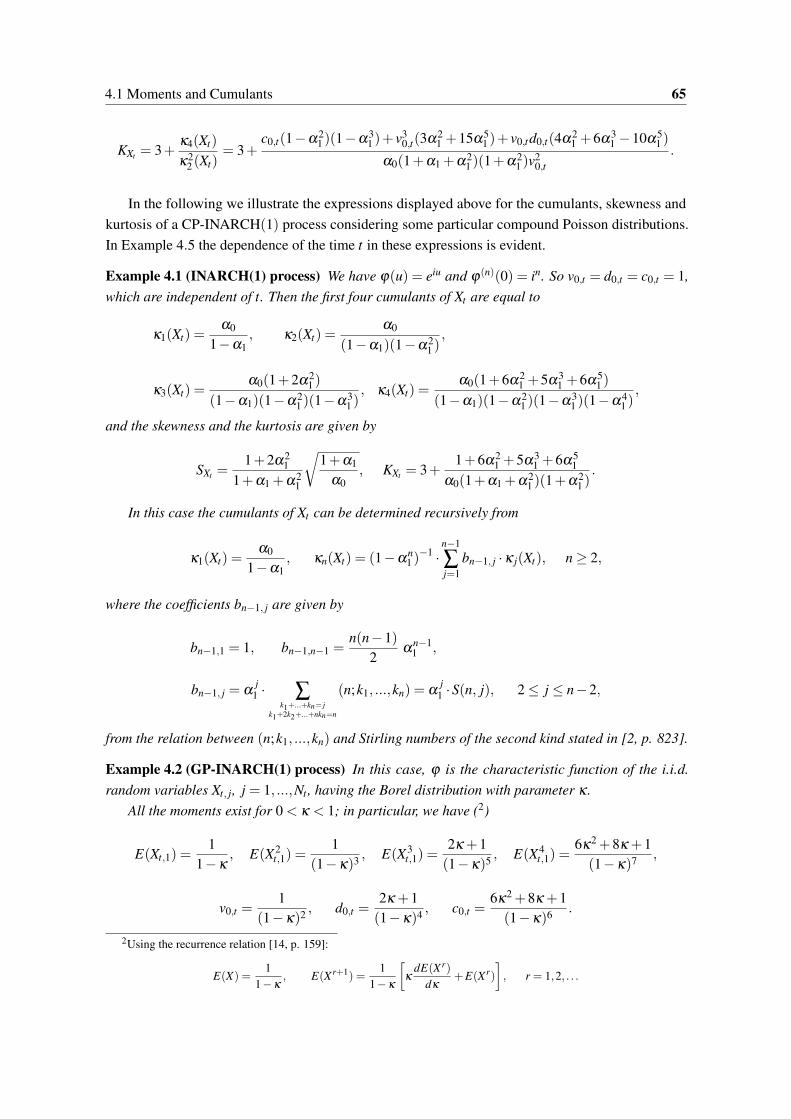
4.1 Moments and Cumulants 65
KXt = 3+κ4(Xt)
κ22 (Xt)
= 3+c0,t(1−α2
1 )(1−α31 )+ v3
0,t(3α21 +15α5
1 )+ v0,td0,t(4α21 +6α3
1 −10α51 )
α0(1+α1 +α21 )(1+α2
1 )v20,t
.
In the following we illustrate the expressions displayed above for the cumulants, skewness andkurtosis of a CP-INARCH(1) process considering some particular compound Poisson distributions.In Example 4.5 the dependence of the time t in these expressions is evident.
Example 4.1 (INARCH(1) process) We have ϕ(u) = eiu and ϕ(n)(0) = in. So v0,t = d0,t = c0,t = 1,which are independent of t. Then the first four cumulants of Xt are equal to
κ1(Xt) =α0
1−α1, κ2(Xt) =
α0
(1−α1)(1−α21 ),
κ3(Xt) =α0(1+2α2
1 )
(1−α1)(1−α21 )(1−α3
1 ), κ4(Xt) =
α0(1+6α21 +5α3
1 +6α51 )
(1−α1)(1−α21 )(1−α3
1 )(1−α41 ),
and the skewness and the kurtosis are given by
SXt =1+2α2
1
1+α1 +α21
√1+α1
α0, KXt = 3+
1+6α21 +5α3
1 +6α51
α0(1+α1 +α21 )(1+α2
1 ).
In this case the cumulants of Xt can be determined recursively from
κ1(Xt) =α0
1−α1, κn(Xt) = (1−α
n1 )
−1 ·n−1
∑j=1
bn−1, j ·κ j(Xt), n ≥ 2,
where the coefficients bn−1, j are given by
bn−1,1 = 1, bn−1,n−1 =n(n−1)
2α
n−11 ,
bn−1, j = αj
1 · ∑k1+...+kn= j
k1+2k2+...+nkn=n
(n;k1, ...,kn) = αj
1 ·S(n, j), 2 ≤ j ≤ n−2,
from the relation between (n;k1, ...,kn) and Stirling numbers of the second kind stated in [2, p. 823].
Example 4.2 (GP-INARCH(1) process) In this case, ϕ is the characteristic function of the i.i.d.random variables Xt, j, j = 1, ...,Nt , having the Borel distribution with parameter κ .
All the moments exist for 0 < κ < 1; in particular, we have (2)
E(Xt,1) =1
1−κ, E(X2
t,1) =1
(1−κ)3 , E(X3t,1) =
2κ +1(1−κ)5 , E(X4
t,1) =6κ2 +8κ +1(1−κ)7 ,
v0,t =1
(1−κ)2 , d0,t =2κ +1(1−κ)4 , c0,t =
6κ2 +8κ +1(1−κ)6 .
2Using the recurrence relation [14, p. 159]:
E(X) =1
1−κ, E(X r+1) =
11−κ
[κ
dE(X r)
dκ+E(X r)
], r = 1,2, . . .
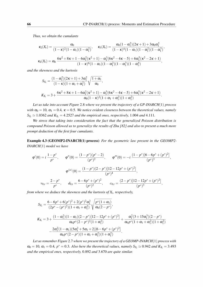
66 CP-INARCH(1) process: Moments and Estimation Procedure
Thus, we obtain the cumulants
κ2(Xt) =α0
(1−κ)2(1−α1)(1−α21 ), κ3(Xt) =
α0(1−α21 )(2κ +1)+3α0α2
1
(1−κ)4(1−α1)(1−α21 )(1−α3
1 ),
κ4(Xt) = α06κ2 +8κ +1−6α2
1 (κ2 +1)−α3
1 (6κ2 −4κ −5)+6α51 (κ
2 −2κ +1)(1−κ)6(1−α1)(1−α2
1 )(1−α31 )(1−α4
1 ),
and the skewness and the kurtosis
SXt =(1−α2
1 )(2κ +1)+3α21
(1−κ)(1+α1 +α21 )
√1+α1
α0,
KXt = 3+6κ2 +8κ +1−6α2
1 (κ2 +1)−α3
1 (6κ2 −4κ −5)+6α51 (κ
2 −2κ +1)α0(1−κ)2(1+α1 +α2
1 )(1+α21 )
.
Let us take into account Figure 2.8 where we present the trajectory of a GP-INARCH(1) processwith α0 = 10, α1 = 0.4, κ = 0.5. We notice evident closeness between the theoretical values, namelySXt ≃ 1.0362 and KXt = 4.2527 and the empirical ones, respectively, 1.004 and 4.111.
We stress that taking into consideration the fact that the generalized Poisson distribution iscompound Poisson allowed us to generalize the results of Zhu [82] and also to present a much moreprompt deduction of the first four cumulants.
Example 4.3 (GEOMP2-INARCH(1) process) For the geometric law present in the GEOMP2-INARCH(1) model we have
ϕ′(0) = i
1− p∗
p∗, ϕ
′′(0) =(1− p∗)(p∗−2)
(p∗)2 , ϕ′′′(0) =−i
(1− p∗)[6−6p∗+(p∗)2]
(p∗)3 ,
ϕ(iv)(0) =
(1− p∗)(2− p∗)[12−12p∗+(p∗)2]
(p∗)4 ,
v0,t =2− p∗
p∗, d0,t =
6−6p∗+(p∗)2
(p∗)2 , c0,t =(2− p∗)[12−12p∗+(p∗)2]
(p∗)3 ,
from where we deduce the skewness and the kurtosis of Xt , respectively,
SXt =6−6p∗+6(p∗)2 +2(p∗)2α2
1
(2p∗− (p∗)2)(1+α1 +α21 )
√p∗(1+α1)
α0(2− p∗),
KXt = 3+(1−α2
1 )(1−α1)(2− p∗)[12−12p∗+(p∗)2]
α0 p∗(2− p∗)2(1+α21 )
+α2
1 (3+15α31 )(2− p∗)
α0 p∗(1+α1 +α21 )(1+α2
1 )
−2α21 (1−α1)(5α2
1 +5α1 +2)[6−6p∗+(p∗)2]
α0 p∗(2− p∗)(1+α1 +α21 )(1+α2
1 ).
Let us remember Figure 2.7 where we present the trajectory of a GEOMP-INARCH(1) process withα0 = 10, α1 = 0.4, p∗ = 0.3. Also here the theoretical values, namely SXt ≃ 0.942 and KXt = 3.493and the empirical ones, respectively, 0.892 and 3.670 are quite similar.

4.1 Moments and Cumulants 67
Example 4.4 (NTA-INARCH(1) process) In this process the skewness and kurtosis are given by
SXt =φ(1−α2
1 )+(1+φ)2(1+2α21 )
(1+φ)(1+α1 +α21 )
√1+α1
α0(1+φ),
KXt = 3+(1−α1)(1−α2
1 )((1+φ)3 +3φ 2 +4φ
)α0(1+α2
1 )(1+φ)2 +(7α2
1 +6α31 +5α5
1 )(1+φ)
α0(1+α1 +α21 )(1+α2
1 )
+φ(4α2
1 +6α31 −10α5
1 )
α0(1+α1 +α21 )(1+α2
1 )(1+φ),
since v0,t = 1+φ , d0,t = 1+3φ +φ 2 and c0,t = 1+7φ +6φ 2 +φ 3.
Example 4.5 Let us recall the model 7(b) defined in Section 2.3 where the conditional distribution isthe binomial Poisson law with parameters (r, 1
t2+1), r ∈N, t ∈ Z, which is deterministic and dependent
of t. In this case we have ϕt(u) =(
t2+eiu
t2+1
)r, u ∈ R, and we can prove
ϕ(n)t (u) = in
n
∑k=1
S(n,k)r!
(r− k)!
(t2 + eiu
t2 +1
)r−k( eiu
t2 +1
)k
, n ∈ N, u ∈ R.
In fact, by induction with respect to n, we have
ϕ(n+1)t (u) =
ddu
(in
n
∑k=1
S(n,k)r!
(r− k)!
(t2 + eiu
t2 +1
)r−k( eiu
t2 +1
)k)
= in+1n
∑k=1
S(n,k)r!
(r− k−1)!
(t2 + eiu
t2 +1
)r−k−1( eiu
t2 +1
)k+1
+in+1n
∑k=1
kS(n,k)r!
(r− k)!
(t2 + eiu
t2 +1
)r−k( eiu
t2 +1
)k
= in+1n+1
∑j=2
[S(n, j−1)+ jS(n, j)]r!
(r− j)!
(t2 + eiu
t2 +1
)r− j( eiu
t2 +1
) j
+S(n,1)r!
(r−1)!
(t2 + eiu
t2 +1
)r−1 eiu
t2 +1
= in+1n+1
∑k=1
S(n+1,k)r!
(r− k)!
(t2 + eiu
t2 +1
)r−k( eiu
t2 +1
)k
, u ∈ R,
from the recurrence relation of the Stirling numbers of the second kind and since S(n,1) = S(n+1,1)(3). Then we deduce
ϕ(n)t (0) = in
n
∑k=1
S(n,k)r!
(r− k)!(t2 +1)k ,
ϕ′t (0) = i
rt2 +1
, ϕ′′t (0) =− r(t2 + r)
(t2 +1)2 , ϕ′′′t (0) =−i
r[(t2 +3r−1)t2 + r2]
(t2 +1)3 ,
3We note that here we use this relation only for the first three moments of the binomial distribution. However, we stateda general expression from which we can obtain the moment of any order.

68 CP-INARCH(1) process: Moments and Estimation Procedure
v0,t =t2 + rt2 +1
, d0,t =(t2 +3r−1)t2 + r2
(t2 +1)2 ,
and finally we obtain the first three cumulants
κ1(Xt) =α0
1−α1, κ2(Xt) =
α0(t2 + r)(t2 +1)(1−α1)(1−α2
1 ),
κ3(Xt) =α0(1−α2
1 )([t2 +3r−1]t2 + r2)+3α0α2
1 (t2 + r)2
(t2 +1)2(1−α1)(1−α21 )(1−α3
1 ),
and the skewness
SXt =(1−α2
1 )([t2 +3r−1]t2 + r2)(t2 +1)3/2 +3α2
1 (t2 + r)2
(t2 + r)3(1+α1 +α21 )
√1+α1
α0(t2 +1)(t2 + r).
In the following theorem we provide closed-form expressions for the joint (central) moments andcumulants of the CP-INARCH(1) model up to order 4 when the family of the characteristic functions(ϕt , t ∈ Z) is deterministic and independent of t. For this purpose, we simply denote the previous v0,t ,c0,t and d0,t respectively as v0, c0 and d0, and we introduce the following notations:
µ(s1, ...,sr−1) = E(XtXt+s1 ...Xt+sr−1
),
µ(s1, ...,sr−1) = E((Xt −µ)(Xt+s1 −µ)...(Xt+sr−1 −µ)
), (4.7)
κ(s1, ...,sr−1) = Cum[Xt ,Xt+s1 , ...,Xt+sr−1
],
with r = 2,3,4 and 0 ≤ s1 ≤ ...≤ sr−1.
Theorem 4.2 (Moments of a CP-INARCH(1) process) Let X be a first-order stationary processfollowing a CP-INARCH(1) model such that H4 is satisfied.
(a) For any k ≥ 0, we have
µ(k) = f2(v0αk1 +α0(1+α1)).
(b) For any l ≥ k ≥ 0, we have
µ(k, l) = [d0(1−α21 )− v2
0(1+α1 −2α21 )] f3α
l+k1
+v0(α0 + v0)
1−α1f2α
l1 + v0 f1 f2α
l−k1 + f1µ(k).
(c) For any m ≥ l ≥ k ≥ 0, we have
µ(k, l,m) = αm−l1
[(c0 −4v0d0 +3v3
0)+3v0(v20 −d0)α1 +(3v0d0 − c0)α
21
+(7v0d0 −6v30 − c0)α
31 +3v0(d0 −2v2
0)α41 +(6v3
0 −6v0d0 + c0)α51
f4α2l+k1
+2v0 +α0
1−α1f3[d0(1−α
21 )− v2
0(1+α1 −2α21 )]
α2l1

4.1 Moments and Cumulants 69
+v0
(1−α1)(1−α21 )
f2[2v0α0 +d0(1−α1)+ v2
0(2α1 −1)]
α2l−k1
+α0 f3
1−α1
d0(1−α
21 )− v2
0(1+α1 −2α21 )
α2(l−k)1 +
v0 +α0
1−α1µ(k, l)
− f2µ(k)[α0 +(v0 +α0)α1]]+ f1µ(k, l).
The proof of Theorem 4.2 is provided in Appendix C.3. These expressions are particularlyimportant to deduce an explicit expression for the asymptotic distribution of the conditional leastsquares estimators of the parameters α0 and α1 in Section 4.2.
From Theorem 4.2 we derive analogous expressions for the joint central moments and cumulantsof a CP-INARCH(1) process. Bakouch [8, p. 5] stated the following general relations between jointmoments and joint cumulants of stationary processes:
κ(s) = µ(s)−µ2, (4.8)
κ(s, l) = µ(s, l)−µµ(s)−µ[µ(l − s)+µ(l)−2µ
2] , (4.9)
κ(s, l,m) = µ(s, l,m)−µµ(s, l)
−µ[µ(l − s,m− s)−µµ(l − s)−µ(l,m)−µµ(l)+µ(s,m)−µµ(s)]
−(µ(s)−µ2)(µ(m− l)−µ
2)− (µ(l)−µ2)(µ(m− s)−µ
2)
−(µ(l − s)−µ2)(µ(m)−µ
2)
+µ2(µ(m)+µ(m− s)+µ(m− l)−3µ
2), (4.10)
where m ≥ l ≥ s ≥ 0. Furthermore, it follows that the joint central moments are given by
µ(s) = E ((Xt −µ)(Xt+s −µ)) = E(XtXt+s)−µ2 = κ(s), (4.11)
µ(s, l) = E[(Xt −µ)(Xt+s −µ)(Xt+l −µ)]
= E[(XtXt+s −µXt −µXt+s +µ2)Xt+l]−µµ(s)
= µ(s, l)−µµ(l)−µµ(s)+µ3 −µµ(s)+µ
3 = κ(s, l), (4.12)
µ(s, l,m) = E[(Xt −µ)(Xt+s −µ)(Xt+l −µ)(Xt+m −µ)]
= E[(XtXt+sXt+l −µXtXt+l −µXt+sXt+l +µ2Xt+l)Xt+m]
−E[(µXtXt+s −µ2Xt −µ
2Xt+s +µ3)Xt+m]−µµ(s, l)
= µ(s, l,m)+µ2[µ(l − s)+µ(m− s)+µ(m− l)+µ(s)+µ(l)+µ(m)]
−µ[µ(l − s,m− s)+µ(l,m)+µ(s, l)+µ(s,m)]−3µ4
= κ(s, l,m)+(µ(s)−µ2)(µ(m− l)−µ
2)+(µ(l)−µ2)(µ(m− s)−µ
2)
+(µ(l − s)−µ2)(µ(m)−µ
2), (4.13)
where m ≥ l ≥ s ≥ 0.
The following corollary may now be enounced.
Corollary 4.2 (Central Moments and Cumulants of a CP-INARCH(1) process) Let X be a first-order stationary process following a CP-INARCH(1) model such that H4 is satisfied.
70 CP-INARCH(1) process: Moments and Estimation Procedure
(a) For any s ≥ 0, we have
µ(s) = κ(s) = v0αs1 f2.
(b) For any l ≥ s ≥ 0, we have
µ(s, l) = κ(s, l)
= f3αl1[v
20(1+α1 +α
21 )−v2
0(1+α1 −2α21 )−d0(1−α
21 )α
s1].
(c) For any m ≥ l ≥ s ≥ 0, we have
κ(s, l,m) = αm1 f4
[c0 +3v3
0 −4v0d0 +3v0(v20 −d0)α1 +(3α0d0 − c0)α
21
+(7v0d0 −6v30 − c0)α
31 +3v0(d0 −2v2
0)α41 +(6v3
0 −6v0d0 + c0)α51
αl+s1
+v0(1+α1 +α21 +α
31 )[d0(1−α
21 )− v2
0(1+α1 −2α21 )](2α
l1 +α
s1)
+v0(1+α1 +α21 )(1+α
21 )[(1+α1)v2
0 +(d0(1−α1)+ v20(2α1 −1))α l−s
1 ]],
µ(s, l,m) = κ(s, l,m)+ v20 f 2
2 αm−l+s1 +2v2
0 f 22 α
m+l−s1 .
The proof of Corollary 4.2 is presented in Appendix C.4. Considering v0, c0 and d0 computedin Examples 4.1–4.4 we obtain the particular expressions of the central moments and cumulantsfor the INARCH(1) (already stated by Weiß [78]), GP-INARCH(1), GEOMP2-INARCH(1) andNTA-INARCH(1) processes.
4.2 Two-step estimation method based on Conditional Least SquaresApproach
This section is intended to derive estimates for the parameters of the CP-INARCH(1) process definedin (4.1) when the family of the characteristic functions (ϕt , t ∈ Z) is independent of t, with specialattention to the recent NTA-INARCH(1) and GEOMP2-INARCH(1) models.
Let X be the referred CP-INARCH(1) process whose distribution depends on a vector θ = (α⊤,b)of unknown parameters, with α⊤ = (α0,α1). Let us observe that, for example, b = φ in the NTA-INARCH(1) model and b = p∗ in the GEOMP2-INARCH(1) model.
Since the conditional law is not specified by its density probability function, we apply a two-stepestimation procedure using the Conditional Least Squares (CLS) and the moments estimation methods:we start by estimating α from the CLS estimator assuming that b is known and then holding thatestimate fixed, we estimate b from the expression of the empirical variance. We shall see that the CLSestimator is computed easily and have an explicit, data-independent expression for the asymptotic law.
Given a set of observations xt , t = 1, ...,n, from a CP-INARCH(1) process according to the aboveconditions, the CLS estimator of α is obtained by minimizing the conditional sum of squares
Qn(α) =n
∑t=2
[xt −E (Xt |Xt−1 = xt−1)]2 =
n
∑t=2
[xt −α0 −α1xt−1]2,

4.2 Two-step estimation method based on Conditional Least Squares Approach 71
with respect to α . Solving the least squares equations
∂Qn(α)
∂α0=−2
n
∑t=2
(xt −α0 −α1xt−1) = 0
∂Qn(α)
∂α1=−2
n
∑t=2
xt−1 (xt −α0 −α1xt−1) = 0,
yields the following explicit expressions for the CLS estimator αn = (α0,n, α1,n):
α1,n =∑
nt=2 XtXt−1 − 1
n−1 ·∑nt=2 Xt ·∑n
s=2 Xs−1
∑nt=2 X2
t−1 −1
n−1 (∑nt=2 Xt−1)
2 , α0,n =∑
nt=2 Xt − α1,n ∑
nt=2 Xt−1
n−1. (4.14)
The consistency and the asymptotic distribution of the CLS estimator αn can be stated by applyingthe results of Klimko and Nelson [50, Section 3]. We summarize the main ideas in the next lemma.
Lemma 4.1 Let X be a stationary and ergodic Markov sequence with finite third order moments. Letus assume that the function g = g(α;Xt−1) = E (Xt |X t−1) satisfies the following regularity conditions:
(i) for i, j,k ∈ 0,1,∂g∂αi
,∂ 2g
∂αi∂α jand
∂ 3g∂αi∂α j∂αk
exist and are continuous for all α;
(ii) for i, j ∈ 0,1, E∣∣∣(Xt −g) ∂g
∂αi
∣∣∣< ∞, E∣∣∣(Xt −g) ∂ 2g
∂αi∂α j
∣∣∣< ∞ and E∣∣∣ ∂g
∂αi· ∂g
∂α j
∣∣∣< ∞, where g andits partial derivatives are evaluated at true value of parameter α and Xt−1;
(iii) for i, j,k ∈ 0,1, there exist functions
H(0) ≡ H(0)(Xt−1, ...), H(1)i ≡ H(1)
i (Xt−1, ...),
H(2)i j ≡ H(2)
i j (Xt−1, ...), H(3)i jk ≡ H(3)
i jk (Xt−1, ...),
such that, for all α ,
|g| ≤ H(0),
∣∣∣∣ ∂g∂αi
∣∣∣∣≤ H(1)i ,
∣∣∣∣ ∂ 2g∂αi∂α j
∣∣∣∣≤ H(2)i j ,
∣∣∣∣ ∂ 3g∂αi∂α j∂αk
∣∣∣∣≤ H(3)i jk ,
E|Xt ·H(3)i jk |< ∞, E
(H(0) ·H(3)
i jk
)< ∞, E
(H(1)
i ·H(2)jk
)< ∞.
Let V be the 2×2 matrix whose (i, j)-th elements are respectively given by
Vi j = E(
∂g(α;Xt−1)
∂αi
∂g(α;Xt−1)
∂α j
), i, j = 1,2.
Then, the CLS estimator αn of α is consistent and asymptotically normal, i.e., as n → ∞
√n(αn −α)
d−→ N(02×1,V−1WV−1),
whenever V is invertible, where " d−→" means convergence in distribution, N(02×1,V−1WV−1) denotesa bivariate normal law with mean vector 02×1 and covariance matrix V−1WV−1 with W being the

72 CP-INARCH(1) process: Moments and Estimation Procedure
2×2 matrix whose (i, j)-th elements are respectively given by
Wi j = E(
u2t (α)
∂g(α;Xt−1)
∂αi
∂g(α;Xt−1)
∂α j
), i, j = 1,2,
and ut(α) = Xt −g(α;Xt−1).
The CP-INGARCH(1) process considered is an ergodic and stationary (Theorem 3.11) Markovchain, since it depends upon its past history only through Xt−1, with all moments finite (Theorem 3.4)and the regularity conditions (i)-(iii) are satisfied. In fact, as g(α;Xt−1) = α0 +α1Xt−1 one obtains
∂g(α;Xt−1)
∂α0= 1,
∂g(α;Xt−1)
∂α1= Xt−1,
∂ 2g(α;Xt−1)
∂αi∂α j=
∂ 3g(α;Xt−1)
∂αi∂α j∂αk= 0, i, j,k = 0,1,
which are continuous for all α , and from where we see that the regularity conditions (i)-(iii) aresatisfied. Thus, from Lemma 4.1, the CLS estimators (4.14) are consistent and asymptotically normal.
Let us obtain the covariance matrix of the asymptotic distribution. We have
V =
E(
∂g∂α0
∂g∂α0
)E(
∂g∂α0
∂g∂α1
)E(
∂g∂α1
∂g∂α0
)E(
∂g∂α1
∂g∂α1
) =
[E (1) E (Xt−1)
E (Xt−1) E(X2
t−1) ]= [ 1 α0
1−α1α0
1−α1
α0(v0+α0(1+α1))
(1−α1)(1−α21 )
],
taking into account the expressions stated in Theorem 4.2. V is invertible and its inverse is equal to
V−1 =(1−α1)(1−α2
1 )
v0α0
[α0(v0+α0(1+α1))
(1−α1)(1−α21 )
− α01−α1
− α01−α1
1
]=
[1+ α0
v0(1+α1) − 1
v0(1−α2
1 )
− 1v0(1−α2
1 )(1−α1)(1−α2
1 )v0α0
].
Furthermore,
E[
f (Xt−1) ·u2t (α)
]= E
[f (Xt−1) ·E
[(Xt −α0 −α1Xt−1)
2|Xt−1]]
= E [ f (Xt−1) ·V [Xt −α0 −α1Xt−1|Xt−1]+0]
= E [ f (Xt−1) ·V [Xt |Xt−1]] = E [ f (Xt−1) · v0(α0 +α1Xt−1)] ,
because of the conditional compound Poisson distribution, and then
W =
E(
u2t
∂g∂α0
∂g∂α0
)E(
u2t
∂g∂α0
∂g∂α1
)E(
u2t
∂g∂α1
∂g∂α0
)E(
u2t
∂g∂α1
∂g∂α1
)
=
[E[1 · v0 (α0 +α1Xt−1)] E[Xt−1 · v0 (α0 +α1Xt−1)]
E[Xt−1 · v0 (α0 +α1Xt−1)] E[X2t−1 · v0 (α0 +α1Xt−1)]
]
=v0α0
1−α1
1 v0α1+α0(1+α1)
1−α21
v0α1+α0(1+α1)
1−α21
v0α0(1+2α1)
(1−α1)(1−α21 )+
α20
(1−α1)2 +α1(d0+(3v2
0−d0)α21 )
(1−α21 )(1−α3
1 )
,

4.2 Two-step estimation method based on Conditional Least Squares Approach 73
since
E[v0 (α0 +α1Xt−1)] = v0
[α0 +α1
α0
1−α1
]=
v0α0
1−α1,
E[Xt−1 · v0 (α0 +α1Xt−1)] = v0
[α2
01−α1
+α1α0(v0 +α0(1+α1))
(1−α1)(1−α21 )
]=
v0α0
1−α1· v0α1 +α0(1+α1)
1−α21
,
E[X2t−1 · v0 (α0 +α1Xt−1)] = v0
[α2
0 (v0 +α0(1+α1))
(1−α1)(1−α21 )
+α1α0
(1−α1)3
(d0 +(3v2
0 −d0)α21
(1+α1)(1+α1 +α21 )
+3v0α0
1+α1+α
20
)]
=v0α0
1−α1
[v0α0(1−α1)+3v0α0α1
(1−α1)2(1+α1)+
α20 (1−α1)+α2
0 α1
(1−α1)2 +α1(d0 +(3v2
0 −d0)α21 )
(1−α21 )(1−α3
1 )
]
=v0α0
1−α1
[v0α0(1+2α1)
(1−α1)(1−α21 )
+α2
0(1−α1)2 +
α1(d0 +(3v20 −d0)α
21 )
(1−α21 )(1−α3
1 )
],
using again the expressions stated in Theorem 4.2.
Now, we provide some calculations to obtain the entries of the matrix V−1WV−1:
The product of V−1W is given by[1+ α0
v0(1+α1) − 1
v0(1−α2
1 )
− 1v0(1−α2
1 )(1−α1)(1−α2
1 )v0α0
] 1 v0α1+α0(1+α1)
1−α21
v0α1+α0(1+α1)
1−α21
v0α0(1+2α1)
(1−α1)(1−α21 )+
α20
(1−α1)2 +α1(d0+(3v2
0−d0)α21 )
(1−α21 )(1−α3
1 )
=
[a11 a12
a21 a22
]=
1−α1v0α11−α2
1− α0α1
1−α1− α1(d0+(3v2
0−d0)α21)
v0(1−α31 )
α1(1−α1)α0
1+α1 +α1(d0+(3v2
0−d0)α21 )
v0α0(1+α1+α21 )
,since
a11 = 1+α0(1+α1)
v0− 1−α2
1v0
v0α1 +α0(1+α1)
1−α21
= 1−α1,
a12 =
(1+
α0
v0(1+α1)
)v0α1 +α0(1+α1)
1−α21
−1−α21
v0
[v0α0(1+2α1)
(1−α1)(1−α21 )
+α2
0(1−α1)2 +
α1(d0 +(3v20 −d0)α
21 )
(1−α21 )(1−α3
1 )
]=
v0α1
1−α21+
α0
1−α1+
α0α1
1−α1+
α20 (1+α1)
v0(1−α1)− α0(1+2α1)
1−α1
−α2
0 (1+α1)
v0(1−α1)−
α1(d0 +(3v20 −d0)α
21 )
v0(1−α31 )
=v0α1
1−α21− α0α1
1−α1−
α1(d0 +(3v2
0 −d0)α21)
v0(1−α31 )
,
a21 = −(1−α21 )
v0+
(1−α1)(1−α21 )(v0α1 +α0(1+α1))
v0α0(1−α21 )
= −(1−α21 )
v0+
α1(1−α1)
α0+
(1−α21 )
v0=
α1(1−α1)
α0,

74 CP-INARCH(1) process: Moments and Estimation Procedure
a22 = −(1−α21 )(v0α1 +α0(1+α1))
v0(1−α21 )
+(1−α1)(1−α2
1 )
v0α0
[v0α0(1+2α1)
(1−α1)(1−α21 )
+α2
0(1−α1)2 +
α1(d0 +(3v20 −d0)α
21 )
(1−α21 )(1−α3
1 )
]= −α1 −
α0(1+α1)
v0+1+2α1 +
α0(1+α1)
v0+
α1(d0 +(3v20 −d0)α
21 )
v0α0(1+α1 +α21 )
= 1+α1 +α1(d0 +(3v2
0 −d0)α21 )
v0α0(1+α1 +α21 )
.
So, the asymptotic covariance matrix is given by
V−1WV−1 =
[b11 b12
b21 b22
]
=v0α0
1−α1
1−α1v0α11−α2
1− α0α1
1−α1− α1(d0+(3v2
0−d0)α21)
v0(1−α31 )
α1(1−α1)α0
1+α1 +α1(d0+(3v2
0−d0)α21 )
v0α0(1+α1+α21 )
[ 1+ α0v0(1+α1) − 1
v0(1−α2
1 )
− 1v0(1−α2
1 )(1−α1)(1−α2
1 )v0α0
]
where
b11 =α0
1−α1
(α0(1+α1)+
v20 +(d0 − v2
0)α1(1+α1 −α21 )+(3v2
0 −d0)α41
v0(1+α1 +α21 )
),
b12 = b21 = v0α1 −α0(1+α1)−α1(1+α1)(d0 +(3v2
0 −d0)α21 )
v0(1+α1 +α21 )
,
b22 = (1−α21 )
(1+
α1(d0 +(3v20 −d0)α
21 )
v0α0(1+α1 +α21 )
).
In fact, we have
b11 =v0α0
1−α1
[(1−α1)
(1+
α0
v0(1+α1)
)− 1
v0(1−α
21 )
(v0α1
1−α21− α0α1
1−α1−
α1(d0 +(3v2
0 −d0)α21)
v0(1−α31 )
)]=
α0
1−α1
[v0(1−α1)+α0(1−α
21 )− v0α1 +α0α1(1+α1)
+α1(d0 +(3v2
0 −d0)α21)(1+α1)
v0(1+α1 +α21 )
]
=α0
1−α1
[α0(1+α1)+
v20(1−2α1)(1+α1 +α2
1 )+α1(d0 +(3v2
0 −d0)α21)(1+α1)
v0(1+α1 +α21 )
]
=α0
1−α1
(α0(1+α1)+
v20 +(d0 − v2
0)α1(1+α1 −α21 )+(3v2
0 −d0)α41
v0(1+α1 +α21 )
),
b12 =v0α0
1−α1
[−(1−α1)(1−α2
1 )
v0
+(1−α1)(1−α2
1 )
v0α0
(v0α1
1−α21− α0α1
1−α1−
α1(d0 +(3v2
0 −d0)α21)
v0(1−α31 )
)]
4.2 Two-step estimation method based on Conditional Least Squares Approach 75
= −α0(1−α21 )+ v0α1 −α0α1(1+α1)−
α1(1+α1)(d0 +(3v2
0 −d0)α21)
v0(1+α1 +α21 )
= v0α1 −α0(1+α1)−α1(1+α1)(d0 +(3v2
0 −d0)α21 )
v0(1+α1 +α21 )
,
b21 =v0α0
1−α1
[α1(1−α1)
α0
(1+
α0(1+α1)
v0
)− 1−α2
1v0
(1+α1 +
α1(d0 +(3v20 −d0)α
21 )
v0α0(1+α1 +α21 )
)]= v0α1 +α0α1(1+α1)−α0(1+α1)−α0α1(1+α1)−
α1(1+α1)(d0 +(3v20 −d0)α
21 )
v0(1+α1 +α21 )
= v0α1 −α0(1+α1)−α1(1+α1)(d0 +(3v2
0 −d0)α21 )
v0(1+α1 +α21 )
,
b22 =v0α0
1−α1
[−α1(1−α1)(1−α2
1 )
v0α0+
(1−α1)(1−α21 )
v0α0
(1+α1 +
α1(d0 +(3v20 −d0)α
21 )
v0α0(1+α1 +α21 )
)]= −α1(1−α
21 )+α1(1−α
21 )+(1−α
21 )
(1+
α1(d0 +(3v20 −d0)α
21 )
v0α0(1+α1 +α21 )
)= (1−α
21 )
(1+
α1(d0 +(3v20 −d0)α
21 )
v0α0(1+α1 +α21 )
).
We have proved the following theorem.
Theorem 4.3 Let αn be the CLS estimate of α given in (4.14). We have
√n(αn −α)
d−→ N(02×1,V−1WV−1),
as n → ∞, where the entries of the matrix V−1WV−1 = (bi j), i, j = 1,2, are those given above.
We carried out simulation studies to illustrate the CLS method for computing the estimates given in(4.14) and also to examine their performance. Table 4.1 presents the computation of the sample meanvalues, and the associated standard errors, for the CLS estimates of α0 and α1 for the INARCH(1)model. These estimates are obtained considering different sample sizes n, namely n = 100, 500,1000, and different combinations of parameters α0 = 0.5, 1, 2 and α1 = 0.2, 0.6, 0.9. We generateda sample of size n for a specified value of the parameters α0 and α1. Then, for this sample size weobtain its CLS estimates. We repeated this procedure 1000 times for these fixed n, α0 and α1, and themean values, along with standard errors in parenthesis, are presented in Table 4.1 (4).
These simulations show that, as expected, the estimates of (α0,α1) perform well as the samplesize increases. For instance, if α0 = 2 and α1 = 0.2, the average of α0 is 2.0434 and the average ofα1 is 0.1815, for n = 100. When the sample size is increased to 1000, the average of the estimates ofα0 and α1 are respectively 2.0012 and 0.1989. Further, the standard errors of the estimates decreasewhen the sample size increases. For the other parameter combinations of α0 and α1 we have a similarbehavior. It is also observed from the Table 4.1 that as α1 decreases, the standard error of the α1
increases and that of α0 decreases. For example, for α0 = 2, we have standard error of α1 equal to0.0741, 0.0949 and 0.1053 (increases) for α1 = 0.9, 0.6, 0.2, respectively. The standard errors of α0,
4The detailed algorithm (in MATLAB code) is given in Appendix D.3.

76 CP-INARCH(1) process: Moments and Estimation Procedure
when α0 = 2, are equal to 1.3762, 0.4676 and 0.2944 (decreases) for α1 = 0.9, 0.6, 0.2, respectively.The standard errors of α0 and α1 behave in a analogous way when α0 decreases.
Table 4.1 CLS estimators performance for the INARCH(1) model-tentativa2.
Parameters n = 100 n = 500 n = 1000α0 α1 Eest(α0) Eest(α1) Eest(α0) Eest(α1) Eest(α0) Eest(α1)
0.2 0.5071 0.1871 0.5033 0.1951 0.5034 0.1954(0.0902) (0.1089) (0.0418) (0.0504) (0.0295) (0.0366)
0.5 0.6 0.5442 0.5527 0.5107 0.5892 0.5071 0.5946(0.1307) (0.1157) (0.0594) (0.0497) (0.0432) (0.0365)
0.9 0.7309 0.8352 0.5611 0.8832 0.5301 0.8921(0.3838) (0.0979) (0.1373) (0.0362) (0.0904) (0.0228)
0.2 1.0134 0.1840 1.0035 0.1967 1.0008 0.1987(0.1582) (0.1072) (0.0711) (0.0477) (0.0496) (0.0333)
1 0.6 1.0809 0.5634 1.0151 0.5926 1.0091 0.5966(0.2465) (0.1027) (0.1099) (0.0447) (0.0757) (0.0308)
0.9 1.4260 0.8524 1.1033 0.8876 1.0483 0.8940(0.7271) (0.0792) (0.2412) (0.0278) (0.1648) (0.0189)
0.2 2.0434 0.1815 2.0068 0.1954 2.0012 0.1989(0.2944) (0.1053) (0.1250) (0.0456) (0.0899) (0.0316)
2 0.6 2.1559 0.5662 2.0177 0.5952 2.0088 0.5982(0.4676) (0.0949) (0.1975) (0.0403) (0.1377) (0.0282)
0.9 2.8086 0.8553 2.1746 0.8903 2.0885 0.8949(1.3762) (0.0741) (0.4791) (0.0259) (0.3153) (0.0177)
Now, we focus on the INARCH(1) model with true parameters α0 = 2 and α1 = 0.2 and, fordifferent sample sizes n = 100, 250, 500, 750, 1000, we present in Table 4.2 the means, variances andcovariance of α0 and α1. In the last column of this table we represent the entries of the asymptoticmatrix V−1WV−1, respectively b11, b22 and b12. It is clear from Table 4.2 (and Table 4.1) that α1 isbiased down and α0 is biased up. The negative covariance between α0 and α1 is a consequence of thisinverse relationship. The asymptotic and the sample values are quite similar for larger values of n.
Table 4.2 Expected values, variances and covariances for the CLS estimates of the INARCH(1) modelfor different sample sizes n and with coefficients α0 = 2 and α1 = 0.2.
n = 100 250 500 750 1000Eest(α0) 2.0434 2.0117 2.0068 2.0037 2.0012Eest(α1) 0.1815 0.1941 0.1954 0.1975 0.1989n ·Vest(α0) 8.3919 8.0550 7.7741 8.0491 8.0647 8.0226n ·Vest(α1) 1.0638 1.0581 1.0267 1.0349 0.9974 1.0436n ·Covest(α0, α1) −2.4616 −2.4310 −2.3139 −2.4114 −2.3783 −2.4090
Until now we have shown how to obtain the CLS estimator for α . To estimate the parameter b weuse a two-step estimation inspired in the moments estimation method. Taking into consideration theexpression of the variance of the CP-INARCH(1) model stated in Remark 3.5, namely
V (Xt) =α0v0
(1−α1)(1−α21 ),

4.2 Two-step estimation method based on Conditional Least Squares Approach 77
we estimate v0 from the estimated equality
α0v0
(1− α1)(1− α21 )
=1n
n
∑t=1
(Xt −Xn
)2,
where Xn =1n ∑
nt=1 Xt denotes the empirical mean of (X1, ...,Xn).
Thus, we deduce the following estimator for the additional parameter present in the
• NTA-INARCH(1) model (since v0 = 1+φ ):
φ =−1+(1− α1)(1− α2
1 )
nα0
n
∑t=1
(Xt −Xn
)2.
• GEOMP2-INARCH(1) model (since v0 =2−p∗
p∗ ):
p∗ = 2
[1+
(1− α1)(1− α21 )
nα0
n
∑t=1
(Xt −Xn
)2
]−1
.
The strong consistence of these estimators is a consequence from the strict stationarity andergodicity of process X . In fact, from the Ergodic Theorem, the empirical variance is a stronglyconsistent estimator for the variance of X which together with the compatibility of the almost sureconvergence with the algebraic operations confirms the statement.
Table 4.3 Expected values, variances and covariances for the CLS estimates of the NTA-INARCH(1)model for different sample sizes n and with coefficients α0 = 2, α1 = 0.2 and φ = 2.
n = 100 250 500 750 1000Eest(α0) 2.0502 2.0078 2.0114 2.0086 2.0058 2Eest(α1) 0.1816 0.1931 0.1939 0.1958 0.1969 0.2Eest(φ) 1.9017 1.9864 1.9861 1.9947 2.0004 2n ·Vest(α0) 12.1944 12.7152 12.4894 12.3982 12.3714 12.3774n ·Vest(α1) 1.2926 1.2501 1.3499 1.2655 1.2836 1.2604n ·Vest(φ) 18.6919 21.9114 23.3308 22.5843 21.3290n ·Covest(α0, α1) −2.4064 −2.5024 −2.7620 −2.5567 −2.4962 −2.5510
Table 4.4 Expected values, variances and covariances for the CLS estimates of the GEOMP2-INARCH(1) model for different sample sizes n and with coefficients α0 = 2, α1 = 0.4 and p∗ = 0.1.
n = 100 250 500 750 1000Eest(α0) 2.0527 2.0758 2.0400 2.0177 2.0182 2Eest(α1) 0.3367 0.3637 0.3817 0.3890 0.3892 0.4Eest(p∗) 0.1170 0.1071 0.1040 0.1026 0.1012 0.1n ·Vest(α0) 50.6433 53.6845 61.9295 56.6796 59.6529 61.5325n ·Vest(α1) 2.9292 3.3704 3.5536 4.2723 3.8424 4.3979n ·Vest(p∗) 0.0961 0.0881 0.0841 0.0856 0.0800n ·Covest(α0, α1) −1.5730 −3.2463 −5.9278 −5.5029 −5.7433 −7.0598
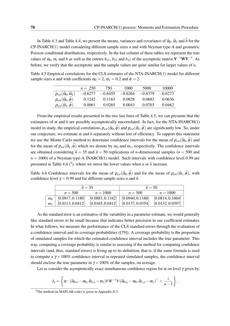
78 CP-INARCH(1) process: Moments and Estimation Procedure
In Table 4.3 and Table 4.4, we present the means, variances and covariance of α0, α1 and b for theCP-INARCH(1) model considering different sample sizes n and with Neyman type-A and geometricPoisson conditional distributions, respectively. In the last column of these tables we represent the truevalues of α0, α1 and b as well as the entries b11, b22 and b12 of the asymptotic matrix V−1WV−1. Asbefore, we verify that the asymptotic and the sample values are quite similar for larger values of n.
Table 4.5 Empirical correlations for the CLS estimates of the NTA-INARCH(1) model for differentsample sizes n and with coefficients α0 = 2, α1 = 0.2 and φ = 2.
n = 250 750 1000 5000 10000ρest(α0, α1) −0.6277 −0.6455 −0.6264 −0.6379 −0.6273ρest(α0, φ) 0.1242 0.1163 0.0828 0.0683 0.0636ρest(α1, φ) 0.0061 0.0265 0.0043 0.0703 0.0462
From the empirical results presented in the two last lines of Table 4.5, we can presume that theestimators of α and b are possibly asymptotically uncorrelated. In fact, for the NTA-INARCH(1)model in study, the empirical correlations ρest(α0, φ) and ρest(α1, φ) are significantly low. So, underour conjecture, we estimate α and b separately without lost of efficiency. To support this statementwe use the Monte Carlo method to determine confidence intervals for the mean of ρest(α0, φ) andfor the mean of ρest(α1, φ) which we denote by m0 and m1, respectively. The confidence intervalsare obtained considering n = 35 and n = 50 replications of n-dimensional samples (n = 500 andn = 1000) of a Neyman type-A INARCH(1) model. Such intervals with confidence level 0.99 arepresented in Table 4.6 (5), where we stress the lower values when n or n increase.
Table 4.6 Confidence intervals for the mean of ρest(α0, φ) and for the mean of ρest(α1, φ), withconfidence level γ = 0.99 and for different sample sizes n and n.
n = 35 n = 50n = 500 n = 1000 n = 500 n = 1000
m0 [0.0917,0.1180] [0.0883,0.1162] [0.0940,0.1160] [0.0814,0.1064]m1 [0.0113,0.0412] [0.0165,0.0412] [0.0137,0.0354] [0.0132,0.0397]
As the standard error is an estimative of the variability in a parameter estimate, we would generallylike standard errors to be small because that indicates better precision in our coefficient estimates.In what follows, we measure the performance of the CLS standard errors through the evaluation ofa confidence interval and its coverage probabilities ([79]). A coverage probability is the proportionof simulated samples for which the estimated confidence interval includes the true parameter. Thisway, computing a coverage probability is similar to assessing if the method for computing confidenceintervals (and, thus, standard errors) is living up to its definition, that is, if the same formula is usedto compute a γ ×100% confidence interval in repeated simulated samples, the confidence intervalshould enclose the true parameter in γ ×100% of the samples, on average.
Let us consider the asymptotically exact simultaneous confidence region for α on level γ given by:
Iγ =
α : (α0,n −α0, α1,n −α1)VW−1V (α0,n −α0, α1,n −α1)
⊤ <z
n−1
,
5The method (in MATLAB code) is given in Appendix D.3.

4.2 Two-step estimation method based on Conditional Least Squares Approach 79
Fig. 4.1 Simultaneous confidence region based on CLS estimates for the INARCH(1) (on the left) andthe NTA-INARCH(1) (on the right, with φ = 2) models with α0 = 2 and α1 = 0.2. Confidence levelγ = 0.9 (lightest gray), 0.95 (lightest and medium gray) and 0.99 (dark to lightest gray).
where z denotes the γ-quantile of the χ22 distribution (6).
Examples of the (non-rectangular) shape of this confidence region for different confidence levelsγ = 0.9, 0.95 and 0.99 are represented in Figure 4.1 with the same true values α0 = 2 and α1 = 0.2.
To estimate the true coverage probability of the confidence region Iγ a simulation study was done.For each combination of true parameters (α0,α1), for each confidence level γ and sample sizes n,10 000 time series were generated. From each time series, the respective estimates and confidenceregion were computed. Then it was checked if this region contained the true parameter tuple. Thenumber of "successes" divided by 10 000 is an estimate of the true coverage probability (7). Theresults are presented in Tables 4.7 to 4.9.
Table 4.7 Estimated coverage probabilities of the confidence region CLS I0.90
γ = 0.90,α0 α1 n = 100 250 500 750 1000 50002 0.2 0.8965 0.8945 0.9007 0.8970 0.9021 0.8977
0.4 0.8816 0.8978 0.8931 0.9021 0.9027 0.90230.6 0.8632 0.8837 0.8880 0.8963 0.8918 0.90050.8 0.8133 0.8609 0.8841 0.8822 0.8889 0.8979
4 0.2 0.8975 0.8997 0.8980 0.8995 0.8961 0.90410.4 0.8859 0.8944 0.8958 0.8983 0.8989 0.89340.6 0.8600 0.8824 0.8917 0.8924 0.8990 0.89420.8 0.8025 0.8543 0.8777 0.8865 0.8881 0.8952
6 0.2 0.8964 0.8971 0.8945 0.8940 0.8981 0.90550.4 0.8860 0.8910 0.8957 0.8939 0.8956 0.89540.6 0.8611 0.8785 0.8913 0.9004 0.8961 0.89660.8 0.8124 0.8631 0.8734 0.8870 0.8882 0.8968
6Let us observe that this confidence region is based on the fact that (Y − µ)⊤Σ−1(Y − µ) is χ2p distributed for a
p-dimensional normal vector Y ∼ N(µ,Σ).7The detailed algorithm (in MATLAB code) is given in Appendix D.3.
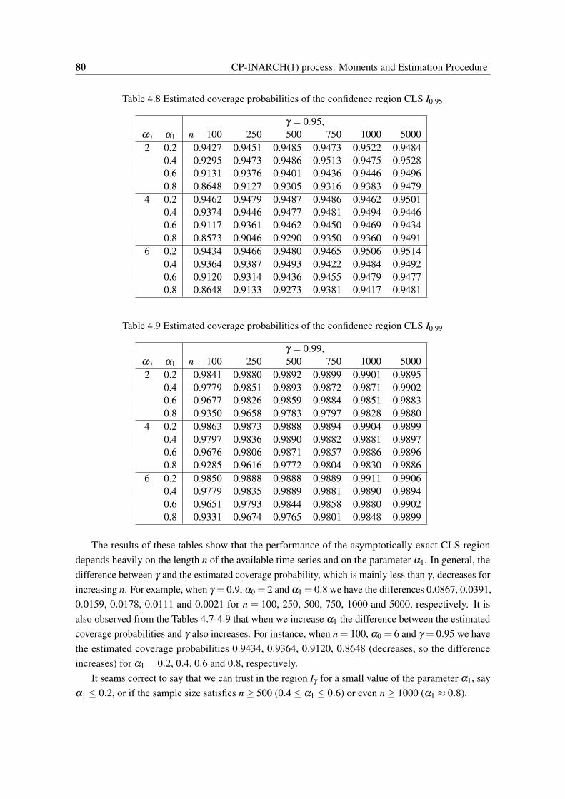
80 CP-INARCH(1) process: Moments and Estimation Procedure
Table 4.8 Estimated coverage probabilities of the confidence region CLS I0.95
γ = 0.95,α0 α1 n = 100 250 500 750 1000 50002 0.2 0.9427 0.9451 0.9485 0.9473 0.9522 0.9484
0.4 0.9295 0.9473 0.9486 0.9513 0.9475 0.95280.6 0.9131 0.9376 0.9401 0.9436 0.9446 0.94960.8 0.8648 0.9127 0.9305 0.9316 0.9383 0.9479
4 0.2 0.9462 0.9479 0.9487 0.9486 0.9462 0.95010.4 0.9374 0.9446 0.9477 0.9481 0.9494 0.94460.6 0.9117 0.9361 0.9462 0.9450 0.9469 0.94340.8 0.8573 0.9046 0.9290 0.9350 0.9360 0.9491
6 0.2 0.9434 0.9466 0.9480 0.9465 0.9506 0.95140.4 0.9364 0.9387 0.9493 0.9422 0.9484 0.94920.6 0.9120 0.9314 0.9436 0.9455 0.9479 0.94770.8 0.8648 0.9133 0.9273 0.9381 0.9417 0.9481
Table 4.9 Estimated coverage probabilities of the confidence region CLS I0.99
γ = 0.99,α0 α1 n = 100 250 500 750 1000 50002 0.2 0.9841 0.9880 0.9892 0.9899 0.9901 0.9895
0.4 0.9779 0.9851 0.9893 0.9872 0.9871 0.99020.6 0.9677 0.9826 0.9859 0.9884 0.9851 0.98830.8 0.9350 0.9658 0.9783 0.9797 0.9828 0.9880
4 0.2 0.9863 0.9873 0.9888 0.9894 0.9904 0.98990.4 0.9797 0.9836 0.9890 0.9882 0.9881 0.98970.6 0.9676 0.9806 0.9871 0.9857 0.9886 0.98960.8 0.9285 0.9616 0.9772 0.9804 0.9830 0.9886
6 0.2 0.9850 0.9888 0.9888 0.9889 0.9911 0.99060.4 0.9779 0.9835 0.9889 0.9881 0.9890 0.98940.6 0.9651 0.9793 0.9844 0.9858 0.9880 0.99020.8 0.9331 0.9674 0.9765 0.9801 0.9848 0.9899
The results of these tables show that the performance of the asymptotically exact CLS regiondepends heavily on the length n of the available time series and on the parameter α1. In general, thedifference between γ and the estimated coverage probability, which is mainly less than γ , decreases forincreasing n. For example, when γ = 0.9, α0 = 2 and α1 = 0.8 we have the differences 0.0867, 0.0391,0.0159, 0.0178, 0.0111 and 0.0021 for n = 100, 250, 500, 750, 1000 and 5000, respectively. It isalso observed from the Tables 4.7-4.9 that when we increase α1 the difference between the estimatedcoverage probabilities and γ also increases. For instance, when n = 100, α0 = 6 and γ = 0.95 we havethe estimated coverage probabilities 0.9434, 0.9364, 0.9120, 0.8648 (decreases, so the differenceincreases) for α1 = 0.2, 0.4, 0.6 and 0.8, respectively.
It seams correct to say that we can trust in the region Iγ for a small value of the parameter α1, sayα1 ≤ 0.2, or if the sample size satisfies n ≥ 500 (0.4 ≤ α1 ≤ 0.6) or even n ≥ 1000 (α1 ≈ 0.8).
Chapter 5
The zero-inflated CP-INGARCH model
In recent years there has been considerable and growing interest in modeling zero-inflated countdata since there is a lot of phenomenon where such data may occur and zero counts frequently havespecial status. With the aim of responding to this kind of data within conditionally heteroscedasticinteger-valued time series we propose a generalization of the CP-INGARCH(p,q) model that maycapture, in addition to the conditional volatility, overdispersion and zero inflation.
The chapter is organized as follows. In Section 5.1 we recall the definition of zero-inflateddistributions and some of their properties. Using this class of distributions we present in Section 5.2the zero-inflated CP-INGARCH model and we specify some particular cases. In parallel to whatwas done in Chapter 3 for the CP-INGARCH model, we analyse first and second-order stationarityconditions in Section 5.3. Moreover, we show how to construct a strictly stationary solution for themodel proposed. We conclude presenting additional probabilistic developments of these processes,particularly, its autocorrelation function and expressions for cumulants.
5.1 Zero-inflated distributions
In some applications the count distribution considered might be inappropriate due to the excess ofzeros in the data compared with what is expected from the distribution. This phenomenon can be aconsequence of the existence of the so called structural zeros. For example, in the counting of thenumber of cigarettes smoked in a day, if the sample includes both smokers and non-smokers, there willbe some of them non-smokers who report 0 cigarettes smoked in a day (meaning they are structuralzeros) and others that did not smoke that day (meaning they are expected or sampling zeros instead).Count data collected from biology is another typical example that contains a lot of zeros. For instance,in counting disease lesions on plants, a plant may have no lesions either because it is resistant to thedisease (structural zeros), or simply because no disease spores have landed on it [67].
Ignoring the excess of zeros, often referred to as zero inflation, we can have at least two conse-quences: first, the estimated parameters and standard errors may be biased, and second, the excessivenumber of zeros can cause overdispersion [87]. To overcome this issue, zero-inflated distributionsshould be specified. These distributions are a two-component mixture where one of the componentsis a point mass at zero and the other component is a count distribution. This way, such distributions
81
82 The zero-inflated CP-INGARCH model
distinguish between structural zeros, for units where zero is the only observable value, and samplezeros, for units on which we observe a zero, but other values might also have been recorded.
Definition 5.1 (Zero-inflated distribution) The probability mass function of a zero-inflated (ZI forbrevity) random variable X can be expressed as
P(X = x) =
ω +(1−ω)P(Y = 0), for x = 0,(1−ω)P(Y = x), for x = 1,2, . . .
(5.1)
where the random variable Y follows a standard count distribution and 0 < ω < 1.
So, the distribution of Y is modified by an additional excess zero function and ω is the proportionof zeros added. Let us observe that these distributions are also referred as zero-modified or withadded zeros [46, p. 351]. It is also possible to take ω less than zero, which corresponds to zerodeflation, provided that ω +(1−ω)P(Y = 0)≥ 0. In the limiting case, that is ω → 0, the zero-inflateddistribution corresponds to the distribution of the random variable Y .
The characteristic function and moments of a zero-inflated distribution can be derived from thoseof the distribution of Y . In fact, if ϕY represents the characteristic function of Y , then
ϕX(u) = E[eiuX]= P(X = 0)+
∞
∑x=1
eiuxP(X = x)
= ω +(1−ω)P(Y = 0)+∞
∑x=1
eiux(1−ω)P(Y = x) = ω +(1−ω)ϕY (u), u ∈ R,
which imply E(X r) = (1−ω)E(Y r), r ∈ N. Thus, the mean and the variance of the zero-inflateddistribution, if they exist, are given respectively by
E(X) = (1−ω)E(Y ) and V (X) = (1−ω)[V (Y )+ω(E(Y ))2].
In the same way, the probability generating function of X is given by gX(z) = ω +(1−ω)gY (z) andits r-th descending factorial moment (1), which can be obtained from g(r)X (1), equals (1−ω)g(r)Y (1).
In addition to being viewed as a mixture, a zero-inflated distribution belongs to the family ofthe compound laws with Bernoulli counting distribution. This means that X can be written asX d= Y1 + ...+YN where N is a Bernoulli random variable with parameter 1−ω (0 < ω < 1) and Yj,
j = 1,2, ..., are i.i.d. random variables which are also independent of N and following the same law asY . In fact, from the proof of Theorem 2.4 the statement holds, i.e., ϕX(u) = ω +(1−ω)ϕY (u), u ∈R.
Regarding its importance within this study, we define in the following the zero-inflated Poisson(ZIP for brevity), the zero-inflated negative binomial (ZINB) and the zero-inflated generalized Poisson(ZIGP) laws. Some other examples of zero-inflated distributions can be found in [46, Section 8.2.4].
Example 5.1 (Zero-inflated Poisson distribution) The random variable X follows a ZIP distribu-tion with parameters (λ ,ω), λ > 0 and 0 < ω < 1, if its probability mass function is given by
1Recall Remark 2.3.

5.1 Zero-inflated distributions 83
P(X = x) =
ω +(1−ω)e−λ for x = 0,
(1−ω)e−λ λ x
x!, for x = 1,2, . . .
Since E(Y ) =V (Y ) = λ , the mean and variance of X are given, respectively, by E(X) = (1−ω)λ
and V (X) = (1−ω)λ (1+ωλ ). In Figure 5.1, we represent the probability mass function of the ZIPdistribution considering different values for the parameters (λ ,ω) from which the effect of increasingthe parameter ω becomes clear.
Fig. 5.1 Probability mass function of X ∼ ZIP(λ ,ω). From the top to the bottom in abscissa x = 4,(λ ,ω) = (4,0) (simple Poisson case with parameter 4), (4,0.3), (4,0.7), (1,0.3).
Example 5.2 (Zero-inflated negative binomial distribution) The random variable X follows a ZINBdistribution with parameters (r, p,ω), r ∈ N, p ∈]0,1[ and 0 < ω < 1, if its probability mass functioncan be written in the form
P(X = x) = ωδx,0 +(1−ω)
(x+ r−1
r−1
)pr (1− p)x , x = 0,1,2, . . . ,
where δx,0 is the Kronecker delta, i.e., δx,0 is 1 when x = 0 and is zero when x = 0. Since themean of the negative binomial distribution is r(1− p)/p and the variance is r(1− p)/p2, we haveE(X) = (1−ω)λ and V (X) = (1−ω)r(1− p)[1+ωr(1− p)]/p2.
Example 5.3 (Zero-inflated generalized Poisson distribution) The random variable X follows aZIGP distribution with parameters (λ ,κ,ω) if its probability mass function can be written in the form
P(X = x) =
ω +(1−ω)e−λ , for x = 0,(1−ω)λ (λ+κx)x−1e−(λ+κx)
x! , for x = 1,2, ...0, for x > m if κ < 0,

84 The zero-inflated CP-INGARCH model
where λ > 0, 0 < ω < 1, max(−1,−λ/m) < κ < 1 and m(≥ 4) is the largest positive integer forwhich λ +κm > 0. Since the mean of the GP law is λ/(1−κ) and the variance is λ/(1−κ)3, we get
E(X) =1−ω
1−κλ and V (X) = (1−ω)
ωλ 2
(1−κ)2 +λ
(1−κ)3
.
5.2 The definition of the ZICP-INGARCH model
Since its introduction [25] the INGARCH model has been generalized and extended in variousdirections in order to increase its flexibility. In Chapter 2 we presented the CP-INGARCH modelas a solution to capture different kind of overdispersion in count data. As reported in literature withexamples from manufacturing defects, road safety, medical consultations or species abundance [67],many count time series also display the zero-inflation characteristic. So, in this Section we will definethe zero-inflated CP-INGARCH model and present some particular cases; a general procedure togenerate this kind of processes will conclude the Section.
Definition 5.2 (ZICP-INGARCH(p, q) model) The process X is said to follow a zero-inflated com-pound Poisson integer-valued GARCH model with orders p and q, (where p,q ∈ N), briefly a ZICP-INGARCH(p,q), if, ∀t ∈ Z, the characteristic function of Xt conditioned on X t−1 is given by
ΦXt |X t−1(u) = ω +(1−ω)exp
i
λt
ϕ ′t (0)
[ϕt(u)−1], u ∈ R, (5.2)
withE(Xt |X t−1)
1−ω= λt = α0 +
p
∑j=1
α jXt− j +q
∑k=1
βkλt−k, (5.3)
for 0 ≤ ω < 1, α0 > 0, α j ≥ 0 ( j = 1, ..., p), βk ≥ 0 (k = 1, ...,q), and where (ϕt , t ∈ Z) is a family ofcharacteristic functions on R, X t−1-measurables, associated to a family of discrete laws with supportin N0 and finite mean. If q = 1 and β1 = 0, the model is simply denoted by ZICP-INARCH(p).
As a consequence of this definition and assuring the existence of variance by considering thatthe characteristic functions (ϕt , t ∈ Z) are twice differentiable at zero, the conditional mean and theconditional variance of Xt are, respectively, given by E(Xt |X t−1) = (1−ω)λt and
V (Xt |X t−1) =−Φ′′Xt |X t−1
(0)− (1−ω)2λ
2t = (1−ω)λt
(−i
ϕ ′′t (0)
ϕ ′t (0)
+ωλt
). (2)
Clearly, the CP-INGARCH model is recovered when ω = 0. Besides this, a wide class of processesis included in the family of ZICP-INGARCH models. To show that, we use the fact that the conditionaldistribution of Xt belongs to the class of the compound laws. In fact, let Mt be a Bernoulli randomvariable with parameter 1−ω , with 0 ≤ ω < 1, and let us define the process X = (Xt , t ∈ Z) as
2Recall the expressions stated in page 18.
5.2 The definition of the ZICP-INGARCH model 85
Xtd=
0, Mt = 0,
Nt
∑j=1
Xt, j, Mt = 1,(5.4)
where, conditionally on X t−1, Nt is a random variable following a Poisson distribution with parameterλ ∗
t = λt/E(Xt, j) and Xt,1, Xt,2,... are discrete random variables with support in N0 and commoncharacteristic function ϕt with finite mean. In addition, all the random variables involved in theequality (5.4) are, for each t, independent. Then the process X satisfies the ZICP-INGARCH modelsince its characteristic function conditioned on X t−1 is given by
ΦXt |X t−1(u) = ω +(1−ω)
∞
∑n=0
E[eiu(Xt,1+...+Xt,Nt ) | Nt = n
]·P(Nt = n)
= ω +(1−ω)e−λ ∗t
∞
∑n=0
ϕnt (u)
(λ ∗t )
n
n!= ω +(1−ω)expλ
∗t [ϕt(u)−1] , u ∈ R.
It should be noted that the ZICP-INGARCH model can also be obtained using another differentrepresentation. Indeed, let us define the process X as
Xtd= Xt,1 + . . .+Xt,Ut , (5.5)
where Ut is a random variable that, conditionally on X t−1, follows a zero-inflated Poisson law and Xt,1,Xt,2, ... are discrete random variables with support in N0 that, conditionally on X t−1, are independent,independent of Ut and with characteristic function ϕt with finite mean. If the parameters of theprobability mass function of Ut are (λ ∗
t ,ω), with λ ∗t = λt/E(Xt, j) and 0 ≤ ω < 1, then the process X
still satisfies the ZICP-INGARCH model as we have
ΦXt |X t−1(u) =
∞
∑n=0
E[expiu(Xt,1 + ...+Xt,Ut )|Ut = n] ·P(Ut = n)
= ω
∞
∑n=0
ϕnt (u)δn,0 +(1−ω)e−λ ∗
t
∞
∑n=0
ϕnt (u)
(λ ∗t )
n
n!
= ω +(1−ω)expλ∗t [ϕt(u)−1] , u ∈ R.
This representation shows that the conditional distribution of the ZICP-INGARCH process can berepresented as a compound distribution with a zero-inflated Poisson law as counting distribution.
We can use any of these representations in law of the model. We remark that representation (5.4)is particularly important in the construction of a strictly stationary solution whereas (5.5) will beuseful to state a condition for the existence of all moments of a ZICP-INGARCH(1,1) model.
Many particular models can be deduced as we illustrate next:
1. To model overdispersion and zero inflation in the same framework, Zhu [84] proposed thezero-inflated Poisson INGARCH(p,q) model (ZIP-INGARCH for brevity) defined as

86 The zero-inflated CP-INGARCH model
Xt | X t−1 ∼ ZIP(λt ,ω) , λt = α0 +p
∑j=1
α jXt− j +q
∑k=1
βkλt−k,
where 0 < ω < 1, α0 > 0, α j ≥ 0, βk ≥ 0, j = 1, ..., p, k = 1, ...,q.
We observe that E(Xt |X t−1) = (1−ω)λt and V (Xt |X t−1) = (1−ω)λt(1+ωλt) (recall Example5.1). This corresponds to a ZICP-INGARCH(p,q) model considering in representation (5.4)λ ∗
t = λt and the characteristic function ϕt(u) = eiu, u ∈ R.
2. In the same paper, Zhu [84] proposed also the zero-inflated negative binomial INGARCH(p,q)process (ZINB-INGARCH for brevity), defined as
Xt | X t−1 ∼ ZINB(
λ1−ct
a,
11+aλ c
t,ω
), λt = α0 +
p
∑j=1
α jXt− j +q
∑k=1
βkλt−k,
where 0 < ω < 1, a > 0, c ∈ 0,1, α0 > 0, α j ≥ 0, βk ≥ 0, j = 1, ..., p, k = 1, ...,q. Wenote that V (Xt |X t−1) = (1−ω)λt(1+ωλt + aλ c
t ) (recall Example 5.2). Considering in therepresentation (5.4), the random variables Xt, j, j = 1,2, ..., having a logarithmic distribution
with parameter aλ ct
1+aλ ct
and λ ∗t = λ
1−cta ln(1+aλ c
t ) we recover the ZINB-INGARCH(p,q) model.
3. Recently, Lee et al. [52] proposed a zero-inflated generalized Poisson autoregressive model(ZIGP AR) by considering
Xt | X t−1 ∼ ZIGP((1−κ)λt ,κ,ω) , λt = f (λt−1,Xt−1),
where 0 ≤ ω < 1, max−1,−(1−κ)λt/m< κ < 1 and f is a positive function on [0,∞[×N0
irrespective of ω and κ . We have V (Xt |X t−1) = (1−ω)λt(1/(1−κ)2 +ωλt) (recall Example5.3) and E(Xt |X t−1) = (1−ω)λt . For 0 < κ < 1 and f (λt−1,Xt−1) = α0 +α1Xt−1 +β1λt−1,we recover a particular case of the ZIGP AR model, which we will called ZIGP-INGARCH,considering that in the representation (5.4) the common distribution of the random variablesXt, j, j = 1,2, ..., is the Borel law with parameter κ and λ ∗
t = (1−κ)λt .
4. Let us consider independent random variables Xt, j, j = 1,2, ..., following a Poisson distributionwith parameter φ > 0 and let Nt follow a Poisson distribution with parameter λ ∗
t = λtφ
, inde-pendent of Xt, j. So, the process X defined as in (5.4) satisfies a ZICP-INGARCH model withV (Xt |X t−1)= (1−ω)λt(1+φ +ωλt) (recall Example 2.4). It is denoted by ZINTA-INGARCH,since the associated conditional law is a zero-inflated Neyman type-A law, i.e.,
Xt | X t−1 ∼ ZINTA(
λt
φ,φ ,ω
), λt = α0 +
p
∑j=1
α jXt− j +q
∑k=1
βkλt−k,
with φ > 0, 0 ≤ ω < 1, α0 > 0, α j ≥ 0, βk ≥ 0, j = 1, ..., p, k = 1, ...,q.
Following the same idea, all the processes defined in Section 2.3 can be extended in order toobtain the ZIGEOMP-INGARCH model, the ZIGEOMP2-INGARCH model, and so on.
Figure 5.2 presents trajectories and the basic descriptives of the ZIP-INGARCH(1,1) modelwith α0 = 10, α1 = 0.4, β1 = 0.5, considering two different values for ω , namely ω = 0.2 and 0.6,

5.2 The definition of the ZICP-INGARCH model 87
illustrating clearly the zero-inflated characteristic of these models (compare with Figure 2.3, whereω = 0). The descriptive resumes presented in Figure 5.2 and Figure 5.3, suggest overdispersion in theclass of the ZICP-INGARCH processes. In fact, for the model specified by (5.2) and (5.3) we have
V (Xt |X t−1)
E(Xt |X t−1)= −i
ϕ ′′t (0)
ϕ ′t (0)
+ωλt =E(X2
t,1)
E(Xt,1)+ωλt
= 1+E(Xt,1(Xt,1 −1))
E(Xt,1)+ωλt ≥ 1+ωλt > 1,
whenever ω > 0, and soV (Xt)
E(Xt)> 1,
that is, the ZICP-INGARCH process is always overdispersed.
Fig. 5.2 Trajectories and descriptives of ZIP-INGARCH(1,1) models with α0 = 10, α1 = 0.4 andβ1 = 0.5: ω = 0.2 (on top) and ω = 0.6 (below).
Fig. 5.3 Trajectory and descriptives of a ZINTA-INGARCH(1,1) model with α0 = 10, α1 = 0.4,β1 = 0.5, φ = 2 and ω = 0.6.
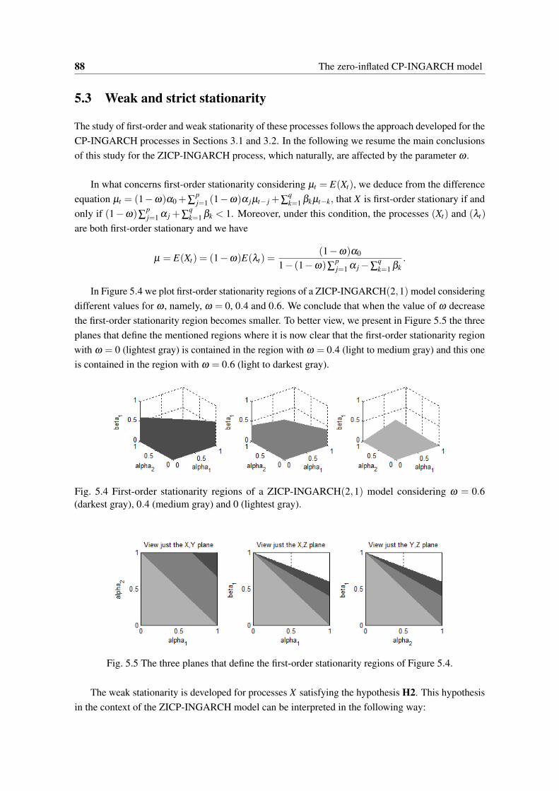
88 The zero-inflated CP-INGARCH model
5.3 Weak and strict stationarity
The study of first-order and weak stationarity of these processes follows the approach developed for theCP-INGARCH processes in Sections 3.1 and 3.2. In the following we resume the main conclusionsof this study for the ZICP-INGARCH process, which naturally, are affected by the parameter ω .
In what concerns first-order stationarity considering µt = E(Xt), we deduce from the differenceequation µt = (1−ω)α0 +∑
pj=1 (1−ω)α jµt− j +∑
qk=1 βkµt−k, that X is first-order stationary if and
only if (1−ω)∑pj=1 α j +∑
qk=1 βk < 1. Moreover, under this condition, the processes (Xt) and (λt)
are both first-order stationary and we have
µ = E(Xt) = (1−ω)E(λt) =(1−ω)α0
1− (1−ω)∑pj=1 α j −∑
qk=1 βk
.
In Figure 5.4 we plot first-order stationarity regions of a ZICP-INGARCH(2,1) model consideringdifferent values for ω , namely, ω = 0, 0.4 and 0.6. We conclude that when the value of ω decreasethe first-order stationarity region becomes smaller. To better view, we present in Figure 5.5 the threeplanes that define the mentioned regions where it is now clear that the first-order stationarity regionwith ω = 0 (lightest gray) is contained in the region with ω = 0.4 (light to medium gray) and this oneis contained in the region with ω = 0.6 (light to darkest gray).
Fig. 5.4 First-order stationarity regions of a ZICP-INGARCH(2,1) model considering ω = 0.6(darkest gray), 0.4 (medium gray) and 0 (lightest gray).
Fig. 5.5 The three planes that define the first-order stationarity regions of Figure 5.4.
The weak stationarity is developed for processes X satisfying the hypothesis H2. This hypothesisin the context of the ZICP-INGARCH model can be interpreted in the following way:

5.3 Weak and strict stationarity 89
−iϕ ′′
t (0)ϕ ′
t (0)=
V (Xt |X t−1)
E(Xt |X t−1)−ωλt .
We stress that, in addition to the examples presented in Section 3.2, the ZIP-INGARCH, the ZINB-INGARCH, the ZIGP-INGARCH and the ZINTA-INGARCH processes also satisfy H2. Namely,
• ZIP-INGARCH(p,q) with v0 = 1;
• ZIGP-INGARCH(p,q) with v0 =1
(1−κ)2 ;
• ZINTA-INGARCH(p,q) with v0 = 1+φ ;
all of them with v1 = 0, and also the
• ZINB-INGARCH(p,q) with
v0 = 1+a and v1 = 0, when c = 0,v0 = 1 and v1 = a, when c = 1.
A necessary and sufficient condition of weak stationarity of X is easily deduced from the vectorialstate space representation presented below. To establish it, let us take into account the following facts:
E(Xt− jλt−k) = E[E(Xt− j|X t− j−1)λt−k
]= (1−ω)E(λt− jλt−k), if k ≥ j, (5.6)
E(Xt− jλt−k) =1
1−ωE [Xt− jE(Xt−k|X t−k−1)] =
E(Xt− jXt−k)
1−ω, if k < j, (5.7)
from where we can deduce the expressions
E(XtXt−h) = E [E(Xt |X t−1)Xt−h] = (1−ω)E(λtXt−h)
= (1−ω)E
([α0 +
p
∑j=1
α jXt− j +q
∑k=1
βkλt−k
]Xt−h
)
= (1−ω)
α0E (Xt−h)+
p
∑j=1
α jE (Xt− jXt−h)+q
∑k=1
βkE (λt−kXt−h)
= (1−ω)
α0E (Xt−h)+
p
∑j=1
α jE (Xt− jXt−h)
+h−1
∑k=1
βk
1−ωE(Xt−kXt−h)+
q
∑k=h
(1−ω)βkE(λt−kλt−h)
, h ≥ 1, (5.8)
and in a similar way
E(λtλt−h) = E
([α0 +
p
∑j=1
α jXt− j +q
∑k=1
βkλt−k
]λt−h
)
= α0E (λt−h)+h
∑j=1
(1−ω)α jE (λt− jλt−h)
+p
∑j=h+1
α j
1−ωE(Xt− jXt−h)+
q
∑k=1
βkE (λt−kλt−h), h ≥ 0. (5.9)
90 The zero-inflated CP-INGARCH model
Proposition 5.1 Suppose that the process X following the ZICP-INGARCH(p,q) model is first-orderstationary and satisfies the hypothesis H2. The vector Wt , t ∈ Z, of dimension p+q−1 given by
Wt =
E(X2t )
E(XtXt−1)
· · ·E(XtXt−(p−1))
E(λtλt−1)
· · ·E(λtλt−(q−1))
satisfies an autoregressive equation of order max(p,q):
Wt = A0 +max(p,q)
∑k=1
AkWt−k, (5.10)
where A0 is a real vector of dimension p+ q− 1 and Ak (k = 1, ...,max(p,q)) are real squaredmatrices of order p+q−1.
Proof: The proof is similar to that of Proposition 3.1. Once again, let us focus on the case p = q.From the hypothesis of first-order stationarity, the expressions (5.6) and (5.7), and since
E(X2t ) = (1−ω)v0E(λt)+(1+ v1)E(λ 2
t ) ⇔ E(λ 2t ) =
E(X2t )− v0µ
(1−ω)(1+ v1),
we deduce the following expressions:
E(X2t ) = D+(1+ v1)
[p
∑j=1
((1−ω)α2
j +2(1−ω)α jβ j +β 2
j
1+ v1
)E(X2
t− j)
+2p−1
∑j=1
p
∑k= j+1
αk((1−ω)α j +β j)E(Xt− jXt−k)
+2(1−ω)p−1
∑j=1
p
∑k= j+1
βk((1−ω)α j +β j)E(λt− jλt−k)
],
E(XtXt−h) =
[α0 −
v0βh
1+ v1
](1−ω)µ +(1−ω)
[αh +
βh
1+ v1
]E(X2
t−h)
+p
∑j=h+1
(1−ω)2β jE(λt− jλt−h)+
p
∑j=h+1
(1−ω)α jE(Xt− jXt−h)
+h−1
∑j=1
((1−ω)α j +β j)E(Xt− jXt−h), h ≥ 1,
E(λtλt−h) =
[α0 −
v0(αh +βh)
1+ v1
]µ
1−ω+
αh +βh
(1−ω)(1+ v1)E(X2
t−h)
+p
∑j=h+1
β jE(λt− jλt−h)+p
∑j=h+1
α j
1−ωE(Xt− jXt−h)
5.3 Weak and strict stationarity 91
+h−1
∑j=1
((1−ω)α j +β j)E(λt− jλt−h), h ≥ 1,
where D = v0µ[1−∑pj=1 (2(1−ω)α jβ j +β 2
j )]+ (1+ v1)[2α0µ −α2
0]
is a positive constant inde-pendent of t. Using these expressions it is clear now that the vector Wt satisfies the autoregressiveequation of order p, Wt = A0 +∑
pk=1 AkWt−k, with A0 = (a j) the vector such that
a j =
D, j = 1,
(1−ω)µ
[α0 −
v0β j−1
1+ v1
], j = 2, ..., p,
µ
1−ω
[α0 −
v0(α j−p +β j−p)
1+ v1
], j = p+1, ...,2p−1,
and Ak (k = 1, ..., p) the squared matrices having generic element a(k)i j given by
• row i = 1:
a(k)1 j =
(1−ω)(1+ v1)α
2k +2(1−ω)αkβk +β 2
k , j = 1,2(1+ v1)[(1−ω)αk +βk]α j+k−1, j = 2, ..., p,2(1−ω)(1+ v1)((1−ω)αk +βk)β j+k−p, j = p+1, ...,2p−1,
• row i = k+1, (k = p):
a(k)k+1, j =
(1−ω)
[αk +
βk
1+ v1
], j = 1,
(1−ω)α j+k−1, j = 2, ..., p,(1−ω)2β j+k−p, j = p+1, ...,2p−1,
• row i = k+ p:
a(k)k+p, j =
αk +βk
(1−ω)(1+ v1), j = 1,
α j+k−1
1−ω, j = 2, ..., p,
β j+k−p, j = p+1, ...,2p−1,
• row i = k+ j:
a(k)k+ j, j =
(1−ω)αk +βk, j = 2, ..., p− k, p+1, ...,2p−1− k,0 j = p− k+1, ..., p,
and for any other case a(k)i j = 0, where we consider α j = β j = 0, for j > p. The general form of thesematrices Ak can be found in Appendix A.2.
In the following theorem we present the referred necessary and sufficient condition for weakstationarity of the ZICP-INGARCH process. The proof is analogous of that of Theorem 3.2.
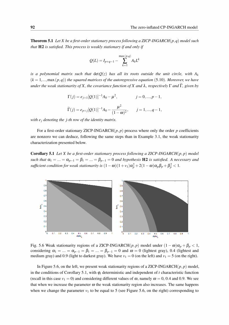
92 The zero-inflated CP-INGARCH model
Theorem 5.1 Let X be a first-order stationary process following a ZICP-INGARCH(p,q) model suchthat H2 is satisfied. This process is weakly stationary if and only if
Q(L) = Ip+q−1 −max(p,q)
∑k=1
AkLk
is a polynomial matrix such that detQ(z) has all its roots outside the unit circle, with Ak
(k = 1,...,max(p,q)) the squared matrices of the autoregressive equation (5.10). Moreover, we haveunder the weak stationarity of X, the covariance function of X and λ , respectively Γ and Γ, given by
Γ( j) = e j+1[Q(1)]−1A0 −µ2, j = 0, ..., p−1,
Γ( j) = ep+ j[Q(1)]−1A0 −µ2
(1−ω)2 , j = 1, ...,q−1,
with e j denoting the j-th row of the identity matrix.
For a first-order stationary ZICP-INGARCH(p, p) process where only the order p coefficientsare nonzero we can deduce, following the same steps than in Example 3.1, the weak stationaritycharacterization presented below.
Corollary 5.1 Let X be a first-order stationary process following a ZICP-INGARCH(p, p) modelsuch that α1 = ... = αp−1 = β1 = ... = βp−1 = 0 and hypothesis H2 is satisfied. A necessary andsufficient condition for weak stationarity is (1−ω)(1+ v1)α
2p +2(1−ω)αpβp +β 2
p < 1.
Fig. 5.6 Weak stationarity regions of a ZICP-INGARCH(p, p) model under (1−ω)αp + βp < 1,considering α1 = ... = αp−1 = β1 = ... = βp−1 = 0 and ω = 0 (lightest gray), 0.4 (lightest andmedium gray) and 0.9 (light to darkest gray). We have v1 = 0 (on the left) and v1 = 5 (on the right).
In Figure 5.6, on the left, we present weak stationarity regions of a ZICP-INGARCH(p, p) model,in the conditions of Corollary 5.1, with ϕt deterministic and independent of t characteristic function(recall in this case v1 = 0) and considering different values of ω , namely ω = 0, 0.4 and 0.9. We seethat when we increase the parameter ω the weak stationarity region also increases. The same happenswhen we change the parameter v1 to be equal to 5 (see Figure 5.6, on the right) corresponding to
5.3 Weak and strict stationarity 93
random characteristics functions ϕt in the ZICP-INGARCH(p, p) model. For instance, these regionscorresponds to a ZINB-INGARCH(1,1) model where a = 5 and c = 1.
In order to derive the autocovariance function of the ZICP-INGARCH(p,q) model, we extendTheorem 3.3 omitting its proof since it is obtained using the same arguments. This general resultincludes those of Zhu [84] on ZIP-INGARCH and ZINB-INGARCH models.
Theorem 5.2 Let X be a weakly stationary ZICP-INGARCH(p,q) process. The autocovariances ofthe processes X and λ satisfy the linear equations
Γ(h) = (1−ω)p
∑j=1
α j ·Γ(h− j)+min(h−1,q)
∑k=1
βk ·Γ(h− k)+(1−ω)2q
∑k=h
βk · Γ(k−h), h ≥ 1,
Γ(h) = (1−ω)min(h,p)
∑j=1
α j · Γ(h− j)+1
1−ω
p
∑j=h+1
α j ·Γ( j−h)+q
∑k=1
βk · Γ(h− k), h ≥ 0,
assuming that ∑qk=h βk · Γ(k−h) = 0 if h > q and ∑
pj=h+1 α j ·Γ( j−h) = 0 if h+1 > p.
The following example illustrate the expression stated for p = q = 1.
Example 5.4 Let X be a ZICP-INGARCH(1,1) model. From Theorem 5.2 we have, for h ≥ 2,
Γ(h) = (1−ω)α1 ·Γ(h−1)+β1 ·Γ(h−1) = ...
= (1−ω)α1 +β1]h−1[(1−ω)α1 ·Γ(0)+(1−ω)2
β1 · Γ(0)].
To determine an expression for V (λt) = Γ(0), we note first that
Γ(h) = (1−ω)α1 · Γ(h−1)+β1 · Γ(h−1) = ...
= [(1−ω)α1 +β1]h · Γ(0), h ≥ 1,
Γ(0) =α1
1−ω·Γ(1)+β1 · Γ(1)
= α21 ·Γ(0)+(1−ω)α1β1 · Γ(0)+β1[(1−ω)α1 +β1] · Γ(0)
= α21 ·Γ(0)+ [2(1−ω)α1β1 +β
21 ] · Γ(0)
⇔ Γ(0) =α2
1 ·Γ(0)1−2(1−ω)α1β1 +β 2
1.
Replacing this in the expression of Γ(h) above, we obtain
Γ(h) = [(1−ω)α1 +β1]h−1 ·
[(1−ω)α1 ·Γ(0)+
(1−ω)2α21 β1 ·Γ(0)
1−2(1−ω)α1β1 +β 21
]= [(1−ω)α1+β1]
h−1 (1−ω)α1[1− (1−ω)α1β1 −β 21 ]
1−2(1−ω)α1β1 −β 21
·Γ(0),

94 The zero-inflated CP-INGARCH model
and so the autocorrelations of X and λ are given by
ρ(h) =Γ(h)Γ(0)
= [(1−ω)α1 +β1]h−1 (1−ω)α1[1− (1−ω)α1β1 −β 2
1 ]
1−2(1−ω)α1β1 −β 21
, h ≥ 1,
ρ(h) = [(1−ω)α1 +β1]h, h ≥ 0.
Under the hypothesis H2, the value of Γ(0) can be deduced, for instance, using the expressionderived in Theorem 5.1. Indeed, Γ(0) =V (Xt) = [Q(1)]−1A0 −µ2, where
Q(1) = 1−A1 = 1− (1−ω)(1+ v1)α21 −2(1−ω)α1β1 −β
21 ,
A0 = v0µ +(1+ v1)[2α0µ − (1−ω)α20 ]− v0µ[2(1−ω)α1β1 +β
21 ],
µ =(1−ω)α0
1− (1−ω)α1 −β1.
Thus, we obtain
Γ(0) =1−2(1−ω)α1β1 −β 2
1
1− (1−ω)(1+ v1)α21 −2(1−ω)α1β1 −β 2
1
(v0µ +
(v1 +ω)µ2
1−ω
).
Using this result when ω = 0 we recover the expression stated in Remark 3.5. When ω = 0, forexample, the variance of the ZINB-INGARCH(1,1) process is given by
Γ(0) =
1−2(1−ω)α1β1−β 2
11−(1−ω)α2
1−2(1−ω)α1β1−β 21
((1+a)µ + ωµ2
1−ω
), c = 0,
1−2(1−ω)α1β1−β 21
1−(1−ω)(1+a)α21−2(1−ω)α1β1−β 2
1
(µ + (a+ω)µ2
1−ω
), c = 1.
Going back to the study of the stationarity properties, we now present the construction of a strictlystationary solution of the ZICP-INGARCH(p,q) model. The study developed in Section 3.4 will beof extreme importance here as well as the representation (5.4) of this process stated in Section 5.2.
With this aim, let us consider a sequence M = (Mt , t ∈ Z) of i.i.d. Bernoulli random variableswith parameter 1−ω , 0 < ω < 1, and let us define a process X∗ = (X∗
t , t ∈ Z) such that
X∗t =
0, Mt = 0,Yt , Mt = 1,
(5.11)
where Y = (Yt , t ∈ Z) is a CP-INGARCH(p,q) process, independent of M, for which the conditionaldistribution of Yt given Y t−1 satisfies
ΦYt |Y t−1(u) = exp
i
λt
ϕ ′t (0)
[ϕt (u)−1], u ∈ R,
E (Yt |Y t−1) = λt = α0 +p
∑j=1
α jYt− j +q
∑k=1
βkλt−k.

5.3 Weak and strict stationarity 95
We remember that in order to have this process it is sufficient to consider Yt = ∑Ntj=1Yt, j where,
conditionally to the past, Nt follows a Poisson law with parameter λt/E(Yt, j) and Yt,1, Yt,2,... arediscrete independent random variables, independent of Nt and with characteristic function ϕt .
If X = (Xt , t ∈ Z) is the process following the model ZICP-INGARCH specified by (5.2) and(5.3), we show in the following that ΦX∗
t |(Y t−1,Mt−1)(u) = ΦXt |X t−1
(u), u ∈ R. In fact, we have
ΦX∗t |(Y t−1,Mt−1)
(u) = E(exp(iuIMt=1Yt
)|(Y t−1,Mt−1)
)= E
(IMt=0+ exp(iuYt)IMt=1|(Y t−1,Mt−1)
)= ω +E
(exp(iuYt)IMt=1|(Y t−1,Mt−1)
)= ω +(1−ω)E (exp(iuYt) |(Y t−1,Mt−1)) , u ∈ R,
since Yt is independent of Mt and Mt are independent variables. So, from the independencebetween the processes Y and M, we obtain
ΦX∗t |(Y t−1,Mt−1)
(u) = ω +(1−ω)E (exp(iuYt) |Y t−1)
= ω +(1−ω)exp
iλt
ϕ′t (0)
[ϕt (u)−1]
= ΦXt |X t−1(u) , u ∈ R.
So, a solution of our ZICP-INGARCH model given by (5.2) and (5.3) may be obtained by (5.11).We are now in conditions to state the strict stationarity of this solution of the model, when ϕt is a
characteristic function deterministic and independent of t.
Theorem 5.3 Let us consider the ZICP-INGARCH(p,q) model as specified in (5.2) and (5.3) andsuch that hypothesis H4 is satisfied. There is a strictly stationary process in L1 that is a solution ofthis model if and only if ∑
pj=1 α j +∑
qk=1 βk < 1. Moreover, this process is also weakly stationary.
Proof: Let us consider the ZICP-INGARCH(p,q) model associated to a deterministic and indepen-dent of t characteristic function ϕ . From Remark 3.8 (b), there is a strictly stationary solution in L1
of a CP-INGARCH(p,q) model associated to the referred characteristic function ϕ if and only if∑
pj=1 α j +∑
qk=1 βk < 1. Let us denote this solution by Y ∗ = (Y ∗
t , t ∈ Z).Then the process X∗ = (X∗
t , t ∈ Z) defined as
X∗t = Y ∗
t IMt=1
with M = (Mt , t ∈ Z) a sequence of i.i.d. Bernoulli random variables with parameter 1−ω , 0 < ω < 1,and independent of Y , is a solution of the ZICP-INGARCH(p,q) model since
ΦX∗t |(Y ∗
t−1,Mt−1)(u) = ω +(1−ω)exp
i
λt
ϕ ′(0)[ϕ(u)−1]
, u ∈ R.
The process X∗ is a strictly stationary process as it is a measurable function of the process(Y ∗
t ,Mt) , t ∈ Z which is strictly stationary as Y ∗ and M are independent and strictly stationaryprocesses. As Y ∗ is a first and a second-order process (Theorem 3.7 and 3.8), the same happens to X∗,and so X∗ is also a weakly stationary process in L1 if ∑
pj=1 α j +∑
qk=1 βk < 1.

96 The zero-inflated CP-INGARCH model
We study now the moments and the cumulants of the ZICP-INGARCH(1,1) process. To this end,let us assume in the following that the characteristic functions ϕt are differentiable as many times asnecessary. We start by enunciating a necessary and sufficient condition for the existence of all itsmoments, a result where the representation (5.5) stated in Section 5.2 will be useful.
Theorem 5.4 The moments of a ZICP-INGARCH(1,1) model satisfying the hypothesis H3 are allfinite if and only if (1−ω)α1 +β1 < 1.
Proof: To prove the statement, let us recall that the conditional distribution of Xt can be viewed as acompound law with a zero-inflated Poisson counting distribution with parameters (λ ∗
t ,ω) providedby the representation (5.5). Since the expression (2.1) presented in Remark 2.3 is valid for anycompound law, and the r-th descending factorial moment of Ut is (1−ω)(λ ∗
t )r, r ≥ 1, we deduce
E[Xmt |X t−1] = (1−ω)
m
∑r=0
1r!
λ rt
(ϕ ′t (0))r
r
∑k=0
(rk
)(−1)r−k
im−r
(ϕ
kt
)(m)(0),
E[Xmt ] = (1−ω)
m
∑r=0
r
∑j=0
1r!
(rj
)(−1)r− j
(ϕ
jt
)(m)(0)
im−r(ϕ ′t (0))r E[λ r
t ], m ≥ 1,
E[λ rt |X t−2] = α
r0 +
r
∑n=1
(rn
)α
r−n0 β
n1 λ
nt−1 +(1−ω)
r
∑n=1
(rn
)α
r−n0
n
∑l=1
(nl
)×
×l
∑v=0
α l1β
n−l1
v!(ϕ ′t−1(0))v
v
∑x=0
(vx
)(−1)v−x
il−v
(ϕ
xt−1)(l)
(0)λ v+n−lt−1 ,
with(ϕk
t)(m) given in Lemma 3.1 and following the same steps as in Theorem 3.4. Then we obtain
the equation E[Λt |X t−2] = d+DΛt−1, with the constant vector d = (αm0 , · · · ,α2
0 ,α0)T and D = (di j),
i, j = 1, ...,m, the upper triangular matrix given by
D =
(1−ω)(α1 +β1)
m +ωβ m1 · · · d1,m−1 d1m
.... . .
......
0 · · · (1−ω)(α1 +β1)2 +ωβ 2
1 dm−1,m
0 · · · 0 (1−ω)α1 +β1
,
from here the required condition holds.
We conclude this section presenting expressions for the first three cumulants and moments up toorder 3 of the ZICP-INARCH(1) model. As in Chapter 4, this study can have interest in statisticaldevelopments of these models. Let us consider a first-order stationary ZICP-INARCH(1) modelsatisfying the hypothesis H4. In the following we illustrate the derivation of its first three cumulants.
Using the characteristic function of the conditional distribution and λt = α0 +α1Xt−1 we obtain
ΦXt (z) = E(eizXt
)= E
[E(eizXt |X t−1
)]

5.3 Weak and strict stationarity 97
= E[
ω +(1−ω)exp
iλt
ϕ ′(0)[ϕ(z)−1]
]= ω +(1−ω)exp
iα0
ϕ ′(0)[ϕ(z)−1]
·ΦXt−1
(α1
ϕ ′(0)[ϕ(z)−1]
)= ω +(1−ω) ·A(z), z ∈ R,
hence, the cumulant generating function of Xt is given by
κXt (z) = ln(ΦXt (z)) = ln(ω +(1−ω) ·A(z)), z ∈ R.
Taking derivatives on both sides, it follows that
κ′Xt(z) =
Φ′Xt(z)
ΦXt (z)=
(1−ω)A′(z)ω +(1−ω)A(z)
=(1−ω)A′(z)
A(z)
(1−ω)+ ω
A(z),
κ′′Xt(z) =
Φ′′Xt(z)
ΦXt (z)−[
Φ′Xt(z)
ΦXt (z)
]2
=(1−ω)A′′(z)
A(z)
(1−ω)+ ω
A(z)−(κ′Xt(z))2,
κ′′′Xt(z) =
Φ′′′Xt(z)
ΦXt (z)−3
Φ′Xt(z)Φ′′
Xt(z)
(ΦXt (z))2 +2
[Φ′
Xt(z)
ΦXt (z)
]3
=(1−ω)A′′′(z)
A(z)
(1−ω)+ ω
A(z)−3κ
′Xt(z)κ ′′
Xt(z)−
(κ′Xt(z))3,
where, taking as h(z) = ϕ(z)−1ϕ ′(0) ,
A′(z) =iα0ϕ ′(z)
ϕ ′(0)· expiα0 ·h(z) ·ΦXt−1 (α1 ·h(z))
+α1ϕ ′(z)ϕ ′(0)
· expiα0 ·h(z) ·Φ′Xt−1
(α1 ·h(z)) ,
A′′(z) =
[iα0ϕ ′′(z)
ϕ ′(0)+
(iα0ϕ ′(z)
ϕ ′(0)
)2]· expiα0 ·h(z) ·ΦXt−1 (α1 ·h(z))
+
[α1ϕ ′′(z)
ϕ ′(0)+2iα0α1
(ϕ ′(z)ϕ ′(0)
)2]· expiα0 ·h(z) ·Φ′
Xt−1(α1 ·h(z))
+
(α1ϕ ′(z)ϕ ′(0)
)2
· expiα0 ·h(z) ·Φ′′Xt−1
(α1 ·h(z)) ,
and
A′′′(z) =
[iα0ϕ ′′′(z)
ϕ ′(0)−3α
20
ϕ ′(z)ϕ ′′(z)(ϕ ′(0))2 − iα3
0
(ϕ ′(z)ϕ ′(0)
)3]· expiα0 ·h(z) ·ΦXt−1 (α1 ·h(z))
+
[6iα0α1
ϕ ′(z)ϕ ′′(z)(ϕ ′(0))2 −3α
20 α1
(ϕ ′(z)ϕ ′(0)
)3
+α1ϕ ′′′(z)ϕ ′(0)
]· expiα0 ·h(z) ·Φ′
Xt−1(α1 ·h(z))

98 The zero-inflated CP-INGARCH model
+
[3α
21
ϕ ′(z)ϕ ′′(z)(ϕ ′(0))2 +3iα0α
21
(ϕ ′(z)ϕ ′(0)
)3]· expiα0 ·h(z) ·Φ′′
Xt−1(α1 ·h(z))
+
(α1ϕ ′(z)ϕ ′(0)
)3
· expiα0 ·h(z) ·Φ′′′Xt−1
(α1 ·h(z)) .
So, we have
A′(z)A(z)
=iα0ϕ ′(z)
ϕ ′(0)+
α1ϕ ′(z)ϕ ′(0)
·κ ′Xt−1
(α1 ·h(z)) ,
A′′(z)A(z)
=iα0ϕ ′′(z)
ϕ ′(0)+
(iα0ϕ ′(z)
ϕ ′(0)
)2
+
[α1ϕ ′′(z)
ϕ ′(0)+2iα0α1
(ϕ ′(z)ϕ ′(0)
)2]·κ ′
Xt−1(α1 ·h(z))
+
(α1ϕ ′(z)ϕ ′(0)
)2
·(
κ′′Xt−1
(α1 ·h(z))+(κ′Xt−1
(α1 ·h(z)))2),
A′′′(z)A(z)
=iα0ϕ ′′′(z)
ϕ ′(0)−
3α20 ϕ ′(z)ϕ ′′(z)(ϕ ′(0))2 − iα3
0
(ϕ ′(z)ϕ ′(0)
)3
+
[6iα0α1
ϕ ′(z)ϕ ′′(z)(ϕ ′(0))2 −3α
20 α1
(ϕ ′(z)ϕ ′(0)
)3
+α1ϕ ′′′(z)ϕ ′(0)
]·κ ′
Xt−1(α1 ·h(z))
+
[3α
21
ϕ ′(z)ϕ ′′(z)(ϕ ′(0))2 +3iα0α
21
(ϕ ′(z)ϕ ′(0)
)3]·(
κ′′Xt−1
(α1 ·h(z))+(κ′Xt−1
(α1 ·h(z)))2)
+
(α1ϕ ′(z)ϕ ′(0)
)3
·[κ′′′Xt−1
(α1 ·h(z))+3κ′Xt−1
(α1 ·h(z))κ′′Xt−1
(α1 ·h(z))+(κ′Xt−1
(α1 ·h(z)))3].
Let us recall the notations stated in (4.6) and the hypothesis of first-order stationarity. Insertingz = 0 into the previous equations and noting that A(0) = 1 and h(0) = 0, we obtain
κ′Xt(0) = (1−ω)
[iα0 +α1 ·κ ′
Xt−1(0)]
⇒ κ1(Xt) = µ =(1−ω)α0
1− (1−ω)α1,
κ′′Xt(0) = (1−ω)
iα0ϕ ′′(0)
ϕ ′(0)−α
20 +
[α1ϕ ′′(0)
ϕ ′(0)+2iα0α1
]·κ ′
Xt−1(0)
+(1−ω)α21 ·[κ′′Xt−1
(0)+(κ′Xt−1
(0))2]− (κ ′
Xt(0))2
−(1−ω)α20 + iv0(1−ω)[iα0 +α1 ·κ ′
Xt−1(0)]+2i(1−ω)α0α1 ·κ ′
Xt−1(0)
+(1−ω)α21 ·[κ′′Xt−1
(0)+(κ′Xt−1
(0))2]+µ
2
= −(1−ω)α20 + iv0 ·κ ′
Xt(0)+2i(1−ω)α0α1 ·κ ′
Xt(0)
+(1−ω)α21 ·κ ′′
Xt−1(0)+(1−ω)α2
1 ·(κ′Xt(0))2
+µ2
5.3 Weak and strict stationarity 99
= (1−ω)α21 ·κ ′′
Xt−1(0)− v0µ
−[(1−ω)α20 +2(1−ω)α0α1µ +(1−ω)α2
1 µ2 −µ
2]
= (1−ω)α21 ·κ ′′
Xt−1(0)− v0µ − ωµ2
1−ω,
since (1−ω)α0 = µ(1− (1−ω)α1), and then, as in Example 5.4,
κ2(Xt) = Γ(0) =v0µ + ωµ2
1−ω
1− (1−ω)α21.
Moreover,
κ′′′Xt(0) = (1−ω)
iα0ϕ ′′′(0)
ϕ ′(0)−
3α20 ϕ ′′(0)ϕ ′(0)
− iα30
+
[6iα0α1
ϕ ′′(0)ϕ ′(0)
−3α20 α1 +α1
ϕ ′′′(0)ϕ ′(0)
]·κ ′
Xt−1(0)
+
[3α
21
ϕ ′′(0)ϕ ′(0)
+3iα0α21
][κ′′Xt−1
(0)+[κ′Xt−1
(0)]2]
+α31 ·[κ′′′Xt−1
(0)+3κ′Xt−1
(0)κ′′Xt−1
(0)+[κ′Xt−1
(0)]3]
−3κ′Xt(0)κ ′′
Xt(0)−
[κ′Xt(0)]3
= −d0(1−ω)[iα0 +α1 ·κ ′Xt−1
(0)]− i(1−ω)α0[3α0v0 +α20 ]
−(1−ω)α1[6α0v0 +3α20 ] ·κ ′
Xt(0)
+3i(1−ω)α21 (v0 +α0) · [κ ′′
Xt(0)+(κ ′
Xt(0))2]
+(1−ω)α31 ·κ ′′′
Xt−1(0)+3(1−ω)α3
1 ·κ ′Xt(0) ·κ ′′
Xt(0)
+(1−ω)α31 · (κ ′
Xt(0))3 +3iµΓ(0)+ iµ3
= (1−ω)α31 ·κ ′′′
Xt−1(0)− id0µ − i(1−ω)α0[3α0v0 +α
20 ]
−(1−ω)iα1[6α0v0 +3α20 ]µ −3i(1−ω)α2
1 (v0 +α0)[Γ(0)+µ2]
−3(1−ω)iα31 µΓ(0)− (1−ω)iα3
1 µ3 +3iµΓ(0)+ iµ3.
Using the equalities
(1−ω)α1µ = µ − (1−ω)α0,
(1−ω)α21 µ
2 = (1−ω)
(µ
1−ω−α0
)2
=µ2
1−ω−2α0µ +(1−ω)α2
0 ,
we deduce
κ′′′Xt(0) = (1−ω)α3
1 ·κ ′′′Xt−1
(0)− id0µ − i(1−ω)α0[3α0v0 +α20 ]
−i[6α0v0 +3α20 ]µ + i(1−ω)α0[6α0v0 +3α
20 ]
−3i(1−ω)α21 (v0 +α0)Γ(0)
+
− 3iµ2
1−ω+6iα0µ −3i(1−ω)α2
0
(v0 +α0)−3iα2
1 Γ(0)µ
100 The zero-inflated CP-INGARCH model
+3i(1−ω)α0α21 Γ(0)− iα1µ3
1−ω+2iα0α1µ
2
−iα20 µ + i(1−ω)α3
0 +3iµΓ(0)+ iµ3
= (1−ω)α31 ·κ ′′′
Xt−1(0)− id0µ −3iv0(1−ω)α2
1 Γ(0)− 3iµ2
1−ω(v0 +α0)
+2iα20 µ −3iα2
1 µΓ(0)− iα1µ3
1−ω+2iα0α1µ
2 +3iµΓ(0)+ iµ3
= (1−ω)α31 ·κ ′′′
Xt−1(0)− id0µ +−3i(1−ω)α2
1 v0Γ(0)
− iωµ2
1−ω[α0 +µ(1+α1)]−3iµ
[v0µ
1−ω−Γ(0)(1−α
21 )
]= (1−ω)α3
1 ·κ ′′′Xt−1
(0)− id0µ −3iv0(1−ω)α21 Γ(0)
− iωµ2
1−ω[α0 +µ(1+α1)]−3iωµ
[µ
1−ω(v0 −µ)+α
21 Γ(0)
]= (1−ω)α3
1 ·κ ′′′Xt−1
(0)− id0µ −3iα21 Γ(0)[(1−ω)v0 +ωµ]
− iωµ2
1−ω[3v0 +α0 +µ(α1 −2)]
and from that we get
κ3(Xt) =d0µ +3α2
1 Γ(0)[(1−ω)v0 −ωµ],+ ωµ2
1−ω[3v0 +α0 +µ(α1 −2)]
1− (1−ω)α31
.
Now we derive an explicit expression for µ(k, l), with 0 ≤ k ≤ l. In order to do this, we rememberthe following conditional moments:
E(Xt |X t−1) = (1−ω)λt = (1−ω)[α0 +α1Xt−1],
E(X2t |X t−1) = (1−ω)
[v0λt +λ
2t]
= (1−ω)[v0(α0 +α1Xt−1)+(α0 +α1Xt−1)
2]= (1−ω)
[α
21 X2
t−1 +α1(v0 +2α0)Xt−1 +α0(v0 +α0)],
and we distinguish the following three cases:
Case 1: l > k.
µ(k, l) = E(XtXt+kXt+l) = E[XtXt+kE(Xt+l|X t+l−1)]
= (1−ω) [α0E(XtXt+k)+α1E(XtXt+kXt+l−1)]
= (1−ω)α0µ(k)+(1−ω)α1µ(k, l −1)
= (1−ω)α0µ(k)+(1−ω)2α1[α0µ(k)+α1µ(k, l −2)]
= (1−ω)α0µ(k)(1+(1−ω)α1)+(1−ω)2α
21 µ(k, l −2)
= . . .= (1−ω)α0µ(k)l−k−1
∑j=0
(1−ω) jα
j1 +(1−ω)l−k
αl−k1 µ(k,k)
= µ ·µ(k)(1− (1−ω)l−kα
l−k1 )+(1−ω)l−k
αl−k1 µ(k,k)

5.3 Weak and strict stationarity 101
= (1−ω)l−kα
l−k1 [µ(k,k)−µ ·µ(k)]+µ ·µ(k).
Case 2: l = k > 0.
µ(k,k) = E[XtE(X2t+k|X t+k−1)]
= (1−ω)[α
21 E(XtX2
t+k−1)+α1(v0 +2α0)E(XtXt+k−1)+α0(v0 +α0)E(Xt)]
= (1−ω)[α
21 µ(k−1,k−1)+α1(v0 +2α0)µ(k−1)+α0(v0 +α0)µ
]= (1−ω)α2
1 µ(k−1,k−1)+(1−ω)kα
k1(v0 +2α0)Γ(0)
+(1−ω)α1(v0 +2α0)µ2 +(1− (1−ω)α1)(v0 +α0)µ
2
= (1−ω)α21 µ(k−1,k−1)+(1−ω)k
αk1(v0 +2α0)Γ(0)
+[α0[1+(1−ω)α1]+ v0]µ2
= (1−ω)α21 µ(k−1,k−1)+(1−ω)k
αk1(v0 +2α0)Γ(0)
+[1− (1−ω)α2
1]
µ ·µ(0)
= . . .= (1−ω)kα
2k1 µ(0,0)+(1−ω)k(v0 +2α0)Γ(0)
k−1
∑j=0
αk+ j1
+[1− (1−ω)α2
1]
µ ·µ(0)k−1
∑j=0
α2 j1
= α2k1
[(1−ω)k
µ(0,0)− v0 +2α0
1−α1(1−ω)k
Γ(0)− (1−ω)µ ·µ(0)]
+v0 +2α0
1−α1(1−ω)k
Γ(0)αk1 +
[1+ω
k−1
∑j=0
α2 j1
]µ ·µ(0).
Case 3: l = k = 0.
µ(0,0) = E(X3t ) = κ3 +3κ2µ +µ
3
=d0µ +3α2
1 κ2[(1−ω)v0 −ωµ]+ ωµ2
1−ω[3v0 +α0 +µ(α1 −2)]
1− (1−ω)α31
+3κ2µ +µ3
=d0µ +κ2[3(1−ω)v0α2
1 −3ωµα21 +2µ −2(1−ω)µα3
1 ]
1− (1−ω)α31
+ωµ2[3v0 +α0 +µ(α1 −2)](1−ω)(1− (1−ω)α3
1 )+µ ·µ(0).


Chapter 6
Conclusions and future developments
"Science never solves a problem without creating ten more." - George Bernard Shaw
This thesis focuses on establishing theoretical results in order to develop applications in whichthe responses are nonnegative integer-valued values, developing a unified study in the class of thenonnegative integer-valued conditional heteroscedastic models. In the last years diverse models havebeen proposed contributing to the existence of a vast literature for analysing count time series. In ouropinion, the work developed under this thesis strongly improves the existing results on this area.
A new class of models which includes the main INGARCH processes present in literature isproposed and developed enlarging and unifying the analysis of those processes, and accomplishingthe practical goal of modeling simultaneously different stylized facts that have been recorded in realcount data: different kinds of conditional heteroscedasticity, overdispersion and zero inflation.
We first proposed a broad class of nonnegative integer-valued conditional heteroscedastic modelsthat is based upon the family of discrete infinitely divisible distributions which incorporates variouswell-known and important distributions. The establishment of the strict stationarity and ergodicity ofthese processes is addressed by presenting the construction of a solution. A necessary and sufficientcondition on the model coefficients for weak stationarity is also stated with some particular casesdisplayed. This general class of processes allows the easy and straightforward introduction of newmodels as well as the inclusion of recent contributions. In fact, a general procedure to obtain thiskind of models is developed showing the main nature of the processes that are solution of the modelequations, namely the fact that they may be expressed, conditioned by the past, as a random sum ofrandom variables. This study resulted in the publication of the paper "Infinitely divisible distributionsin integer-valued GARCH models" [34]. Moreover, an overall estimation procedure based on theconditional least squares and on the moments estimation method is analysed in this thesis.
Among the new models that can be presented and because of its practical potential, we underlinein the paper "A new approach to integer-valued times series modeling: The Neyman Type-A INGARCHmodel" [33] the study of the particular Neyman Type-A INGARCH model.
Thereafter, it seemed to be natural to consider zero-inflated conditional distributions in the previousmodel in order to take also into account in the same framework the characteristic of zero inflation. Thisgeneralization of the CP-INGARCH model was analysed recently in "Zero-inflated compound Poissondistributions in integer-valued GARCH models" [35]. The previous study plays an important role
103
104 Conclusions and future developments
mainly to state strict stationarity. In addition, the autocorrelation function, expressions for momentsand cumulants and a condition ensuring the finiteness of the moments of the process are treated.
Although some of the particular models of the ZICP-INGARCH process have already probabilisticdevelopments, our study, in many cases, enlarges or completes them. For instance, in Example 4.2 wecomputed the first four cumulants, the skewness and the kurtosis of the GP-INARCH(1) model. Aswe mentioned, Zhu [82] only presented the mean and the variance claiming the difficulty for derivinghigher-order cumulants with the techniques adopted. For the ZIP-INGARCH model defined by Zhu[84] we provide an important contribution on the stationarity. In fact, from Theorem 5.3 the strictstationarity is analysed displaying a solution whereas in the literature, to the best of our knowledge,only first and second-order stationarity conditions were established ([84]) and the strict stationarity forp = q = 1 ([52]), by using different techniques than ours. Another example is the NB-DINARCH(p)model. Xu et al. [80] presented a sufficient condition for the strictly stationarity and ergodicity of theprocess but a solution was not shown. We answered it in Theorem 3.11. New results for this model,for p = 1, are presented as the existence of all moments (Theorem 3.4) and expressions for momentsand cumulants (Theorem 4.2 and Corollary 4.2). For the NB-INGARCH model, Zhu [81] proposed anecessary and sufficient condition for the weak stationarity analogous to the necessary condition forthe weak stationarity of our model presented in Appendix B. Nevertheless, we stress that the studydeveloped to discuss the weak stationarity of our general model follows a new vectorial approach.
Other probabilistic studies may be considered in future as, for instance, those related to the Taylorproperty ([32]), the behavior of the tails or the analysis of the strict stationarity of this model when ϕt
is a random function which is still an open question that deserves further development. The estimationof the distribution of a ZICP-INGARCH process is also a subject of future interest. To evaluateit by bounding as for real heteroscedastic processes, ([61]), could be a first approach. In Section4.2, we presented a preliminary study on the estimation of the model parameters. In the simulationstudy presented, the empirical results lead us to think that the proposed estimators of α and b areasymptotically uncorrelated, an assertion which requires theoretical developments as well as theproperties of the estimator b. It seems also interesting to develop alternative parameters estimatemethods, for example, using a Poisson quasi-maximum likelihood estimator ([3]).
This work can be viewed as a starting point for new extensions of the INGARCH model. Oneof them will be to consider instead of a conditional compound Poisson distribution other particularcompound distributions such as the compound negative binomial or the compound binomial. Usingthe same methodology and slightly heavier calculations, the study presented can also be made when adiscrete set of points present probability inflation. Different specifications for the conditional meancan also be considered. More specifically we can assume, for example, a two-regime structure of theconditional mean process according to the magnitude of the lagged observations (similar to Wanget al. [75] who proposed the self-excited threshold integer-valued Poisson autoregressive model); thecoefficients α’s and β ’s of the evolution of the conditional mean being periodic in t, with a certainperiod S (similar to Bentarzi and Bentarzi [9] who investigated the periodic INGARCH model); orthe conditional mean of the form λt = f (λt−1,Xt−1), with the function f defined on [0,∞[×N0 (as in[52]).
References
[1] Abramowitz, M. and Stegun, I. (1965a). Handbook of Mathematical Functions. Dover Publica-tions, Inc., New York.
[2] Abramowitz, M. and Stegun, I. (1965b). Handbook of Mathematical Functions. Dover Publica-tions, Inc., New York.
[3] Ahmad, A. and Francq, C. (2015). Poisson QMLE of count time series models. Journal of TimeSeries Analysis, page DOI: 10.1111/jtsa.12167.
[4] Al-Osh, M. and Alzaid, A. (1987). First-order integer-valued autoregressive (INAR(1)) process.Journal of Time Series Analysis, 8(3):261–275.
[5] Al-Osh, M. and Alzaid, A. (1988). Integer-valued moving average (INMA) process. Statist.Papers, 29:281–300.
[6] Alzaid, A. and Al-Osh, M. (1988). First-order integer-valued autoregressive process: distributionaland regression properties. Statistica Neerlandica, 42:53–61.
[7] Azencott, R. and Dacunha-Castelle, D. (1984). Séries d’observations irrégulières, modélisationet prévision. Masson, Paris.
[8] Bakouch, H. (2010). Higher-order moments, cumulants and spectral densities of the NGINAR(1)process. Statistical Methodology, 7:1–21.
[9] Bentarzi, M. and Bentarzi, W. (2015). Periodic Integer-Valued GARCH(1,1) Model. Communica-tions in Statistics - Simulation and Computation, DOI:10.1080/03610918.2014.994780.
[10] Bollerslev, T. (1986). Generalized autoregressive conditional heteroscedasticity. Journal ofEconometrics, 37:307–327.
[11] Brännäs, K. and Hall, A. (2001). Estimation in integer-valued moving average models. Appl.Stochastic Models Bus. Ind., 17:277–291.
[12] Brockwell, P. and Davis, R. (1991). Time series: Theory and Methods. Springer-Verlag, NewYork, 2nd edition.
[13] Christou, V. and Fokianos, K. (2014). Quasi-likelihood inference for negative binomial timeseries model. Journal of Time Series Analysis, 35:55–78.
105
106 References
[14] Consul, P. C. and Famoye, F. (2006). Lagrangian Probability Distributions. Birkhäuser, Boston.
[15] Cramér, H. (1946). Mathematical Methods of Statistics. Princeton University Press, Princeton.
[16] Davis, R. and Liu, H. (2015). Theory and inference for a class of observation-driven time seriesmodels with application to time series of counts. Forthcoming in Statistica Sinica.
[17] de Finetti, B. (1929). Sulle funzioni ad incremento aleatorio. Rend. Acad. Lincei., 10:163–168.
[18] Doukhan, P., Latour, A., and Oraichi, D. (2006). A simple Integer-Valued bilinear time seriesmodel. Adv. Appl. Prob., 38:559–578.
[19] Drost, F., van den Akker, R., and Werker, B. (2008). Note on Integer-Valued bilinear time seriesmodels. Stat. and Prob. Letters, 78:992–996.
[20] Du, J. and Li, Y. (1991). The integer-valued autoregressive (INAR(p)) model. Journal of TimeSeries Analysis, 12:129–142.
[21] Efron, B. (1986). Double exponential families and their use in generalized linear regression.Journal of the American Statistical Association, 81:709–721.
[22] Elaydi, S. (2005). An Introduction to difference equations. Springer Science+Business Media,Inc., New York, 3rd edition.
[23] Engle, R. and Russell, J. (1998). Autoregressive conditional duration: a new model for irregularlyspaced transaction data. Econometrica, 66(5):1127–1162.
[24] Feller, W. (1968). An Introduction to Probability Theory and Its Applications, volume 1. Wiley,New York, 3rd edition.
[25] Ferland, R., Latour, A., and Oraichi, D. (2006). Integer-valued GARCH process. Journal ofTime Series Analysis, 27:923–942.
[26] Fokianos, K., Rahbek, A., and Tjøtheim, D. (2009). Poisson autoregression. Journal of theAmerican Statistical Association, 104:1430–1439.
[27] Freeland, R. and McCabe, B. (2004). Forecasting discrete valued low count time series. Interna-tional Journal of Forecasting, 20:427–434.
[28] Fristedt, B. and Gray, L. (1997). A Modern Approach to Probability Theory. Birkhauser, Boston.
[29] Gantmacher, F. (1959). The theory of matrices, volume I. Chelsea, New York.
[30] Gauthier, G. and Latour, A. (1994). Convergence forte des estimateurs des paramètres dt’unprocessus GENAR(p). Annales des Sciences Mathématiques du Québec, 18:49–71.
[31] Gnedenko, B. and Kolmogorov, A. (1954). Limit Distributions for Sums of Independent RandomVariables. Addison-Wesley, Reading, Mass.
[32] Gonçalves, E., Leite, J., and Mendes Lopes, N. (2009). A mathematical approach to detect theTaylor property in TARCH processes. Stat. and Prob. Letters, 72:602–610.
References 107
[33] Gonçalves, E., Mendes Lopes, N., and Silva, F. (2015a). A new approach to integer-valuedtimes series modeling: The Neyman Type-A INGARCH model. Lithuanian Mathematical Journal,55(2):231–242.
[34] Gonçalves, E., Mendes Lopes, N., and Silva, F. (2015b). Infinitely divisible distributions ininteger-valued GARCH models. Journal of Time Series Analysis, 36:503–527.
[35] Gonçalves, E., Mendes Lopes, N., and Silva, F. (2016). Zero-inflated compound Pois-son distributions in integer-valued GARCH models. To appear in Statistics, page DOI:10.1080/02331888.2015.1114622.
[36] Gouriéroux, C. and Monfort, A. (1990). Séries temporelles et modèles dynamiques. Economica,Paris.
[37] Grahramani, M. and Thavaneswaran, A. (2009). On some properties of Autoregressive Condi-tional Poisson (ACP) models. Economic Letters, 105:273–275.
[38] Grandell, J. (1997). Mixed Poisson Processes. Chapman & Hall, London.
[39] Grubbström, R. and Tang, O. (2006). The moments and central moments of a compounddistribution. European Journal of Operational Research, 170:106–119.
[40] Heinen, A. (2003). Modelling Time Series Count Data: An Autoregressive Conditional PoissonModel. CORE Discussion Paper, 2003-63, University of Louvain, Belgium.
[41] Horn, R. A. and Jonhson, C. R. (2013). Matrix Analysis. Cambridge University Press, NewYork, 2nd edition.
[42] Hu, C., Iksanov, A., Lin, G., and Zakusylo, O. (2006). The Hurwitz Zeta Distribution. Aust. N.Z. J. Stat., 48(1):1–6.
[43] Jacobs, P. and Lewis, P. (1978a). Discrete time series generated by mixtures I: Correlational andruns properties. J. Roy. Statist. Soc. B, 40:94–105.
[44] Jacobs, P. and Lewis, P. (1978b). Discrete time series generated by mixtures II: Asymptoticproperties. J. Roy. Statist. Soc. B, 40:222–228.
[45] Jadi, M., Jones, G., and Lai, C. (2012). First-order integer valued AR processes with zeroinflated Poisson innovations. Journal of Time Series Analysis, 33(6):954–963.
[46] Johnson, N. L., Kotz, S., and Kemp, A. W. (2005). Univariate discrete distributions. Wiley,New York, 3rd edition.
[47] Kachour, M. (2014). On the Rounded Integer-Valued Autoregressive Process. Communicationsin Statistics - Theory and Methods, 43:355–376.
[48] Kachour, M. and Yao, J. (2009). First-order rounded integer-valued autoregressive (RINAR(1))process. Journal of Time Series Analysis, 30(4):417–448.
108 References
[49] Kachoura, M. and Truquet, L. (2011). A p-Order signed integer-valued autoregressive(SINAR(p)) model. Journal of Time Series Analysis, 32:223–236.
[50] Klimko, L. and Nelson, P. (1978). On conditional least squares estimation for stochasticprocesses. Ann. Stat., 6(3):629–642.
[51] Kress, R. (1998). Numerical Analysis. Springer, New York.
[52] Lee, S., Lee, Y., and Chen, C. (2015). Parameter change test for zero-inflated generalizedPoisson autoregressive models. Statistics, page DOI: 10.1080/02331888.2015.1083020.
[53] Lukacs, E. (1964). Fonctions Caractéristiques. Dunod, Paris.
[54] McKenzie, E. (1985). Some simple models for discrete variate time series. Water ResourcesBulletin, 21(4):645–650.
[55] McKenzie, E. (1988). Some ARMA models for dependent sequences of Poisson counts. Adv.Appl. Probab., 20:822–835.
[56] Neumann, M. (2011). Absolute regularity and ergodicity of Poisson count processes. Bernoulli,17:1268–1284.
[57] Neyman, J. (1939). On a new class of “contagious” distributions applicable in entomology andbacteriology. Annals of Mathematical Statistics, 10:35–57.
[58] Nolan, J. (2006). Stable Distributions- Models for Heavy Tailed Data. Birkhauser.
[59] Özel, G. and Inal, C. (2010). The probability function of a geometric Poisson distribution.Journal of Statistical Computation and Simulation, 80(5):479–487.
[60] Panjer, H. (2006). Operational Risks: Modeling Analytics. John Wiley & Sons, New York.
[61] Pawlak, M. and Schmid, W. (2001). On the distributional properties of GARCH processes.Journal of Time Series Analysis, 22(3):339–352.
[62] Perumean-Chaney, S., Morgan, C., and McDowall, D. (2013). Zero-inflated and overdispersed:What´s one to do? Journal of Statistical Computation and Simulation, 83(9):1671–1683.
[63] Pólya, G. (1930). Sur quelques points de la théorie des probabilités. Annales de l’Institut H.Poincaré, 1:117–161.
[64] Quarteroni, A., Sacco, R., and Saleri, F. (2000). Numerical Mathematics. Texts in AppliedMathematics 37, Springer-Verlag, New York, 2nd edition.
[65] Resnick, S. (1998). A probability Path. Birkhauser, Boston.
[66] Ridout, M. and Berbeas, P. (2004). An empirical model for underdispersed count data. StatisticalModelling, 4:77–89.

References 109
[67] Ridout, M., Demétrio, C., and Hinde, J. (1998). Models for count data with many zeros. In:Proceedings of the 19th International Biometrics Conference, Cape Town, South Africa, pages179–190.
[68] Rosenblatt, M. (1978). Dependence and asymptotic independence for random processes. Studiesin Probability Theory, The Mathematical Association of America.
[69] Shmueli, G., Minka, T., Kadane, J., Borle, S., and Boatwright, P. (2005). A useful distributionfor fitting discrete data: revival of the Conway-Maxwell-Poisson distribution. Applied Statistics,54:127–142.
[70] Silva, M. and Oliveira, V. (2004). Difference equations for the higher-order moments andcumulants of the INAR(1) model. Journal of Time Series Analysis, 25(3):317–333.
[71] Silva, M. and Oliveira, V. (2005). Difference equations for the higher-order moments andcumulants of the INAR(p) model. Journal of Time Series Analysis, 26:17–36.
[72] Steutel, F. and van Harn, K. (1979). Discrete analogues of self-decomposability and stability.The Annals of Probability, 7(5):893–899.
[73] Steutel, F. W. and van Harn, K. (2004). Infinitely divisibility of probability distributions on thereal line. Marcel Dekker, Inc., New York.
[74] Turkman, K., Scotto, M., and Bermudez, P. Z. (2014). Non-Linear Time Series - Extreme Eventsand Integer Value Problems. Springer, New York.
[75] Wang, C., Liu, H., Yao, J.-f., Davis, R., and Li, W. (2014). Self-Excited Threshold PoissonAutoregression. Journal of the American Statistical Association, 109(506):777–787.
[76] Weiß, C. (2008). Thinning operations for modelling time series of counts- a survey. Adv. Stat.Anal., 92:319–341.
[77] Weiß, C. (2009). Modelling time series of counts with overdispersion. Statistical Methods andApplications, 18:507–519.
[78] Weiß, C. (2010a). INARCH(1) Processes: Higher-order Moments and Jumps. Stat. Probab.Lett., 80:1771–1780.
[79] Weiß, C. (2010b). The INARCH(1) model for overdispersed time series of counts. Communica-tions in Statistics - Simulation and Computation, 39:1269–1291.
[80] Xu, H.-Y., Xie, M., Goh, T. N., and Fu, X. (2012). A model for integer-valued time series withconditional overdispersion. Computational Statistics and Data Analysis, 56:4229–4242.
[81] Zhu, F. (2011). A negative binomial integer-valued GARCH model. Journal of Time SeriesAnalysis, 32:54–67.
[82] Zhu, F. (2012a). Modeling overdispersed or underdispersed count data with generalized Poissoninteger-valued GARCH models. Journal of Mathematical Analysis and Applications, 389(1):58–71.

110 References
[83] Zhu, F. (2012b). Modeling time series of counts with COM-Poisson INGARCH models.Mathematical and Computer Modelling, 56:191–203.
[84] Zhu, F. (2012c). Zero-inflated Poisson and negative binomial integer-valued GARCH models. J.of Stat. Plann. and Inf., 142:826–839.
[85] Zhu, F. and Wang, D. (2010). Diagnostic checking integer-valued ARCH(p) models usingconditional residual autocorrelations. Comput. Stat. Data Anal., 54:496–508.
[86] Zhu, F. and Wang, D. (2011). Estimation and testing for a Poisson autoregressive model. Metrika,73:211–230.
[87] Zuur, A., Ieno, E., Walker, N., Saveliev, A., and Smith, G. (2009). Mixed Effects Models andExtensions in Ecology with R. Springer, New York.
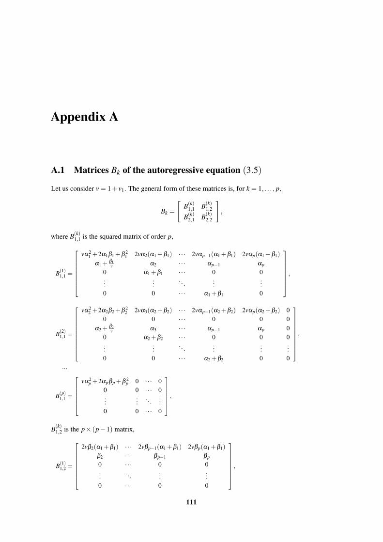
Appendix A
A.1 Matrices Bk of the autoregressive equation (3.5)
Let us consider v = 1+ v1. The general form of these matrices is, for k = 1, . . . , p,
Bk =
[B(k)
1,1 B(k)1,2
B(k)2,1 B(k)
2,2
],
where B(k)1,1 is the squared matrix of order p,
B(1)1,1 =
vα2
1 +2α1β1 +β 21 2vα2(α1 +β1) · · · 2vαp−1(α1 +β1) 2vαp(α1 +β1)
α1 +β1v α2 · · · αp−1 αp
0 α1 +β1 · · · 0 0...
.... . .
......
0 0 · · · α1 +β1 0
,
B(2)1,1 =
vα22 +2α2β2 +β 2
2 2vα3(α2 +β2) · · · 2vαp−1(α2 +β2) 2vαp(α2 +β2) 00 0 · · · 0 0 0
α2 +β2v α3 · · · αp−1 αp 0
0 α2 +β2 · · · 0 0 0...
.... . .
......
...0 0 · · · α2 +β2 0 0
,
...
B(p)1,1 =
vα2
p +2αpβp +β 2p 0 · · · 0
0 0 · · · 0...
.... . .
...0 0 · · · 0
,
B(k)1,2 is the p× (p−1) matrix,
B(1)1,2 =
2vβ2(α1 +β1) · · · 2vβp−1(α1 +β1) 2vβp(α1 +β1)
β2 · · · βp−1 βp
0 · · · 0 0...
. . ....
...0 · · · 0 0
,
111

112
B(2)1,2 =
2vβ3(α2 +β2) · · · 2vβp−1(α2 +β2) 2vβp(α2 +β2) 00 · · · 0 0 0β3 · · · βp−1 βp 00 · · · 0 0 0...
. . ....
......
0 · · · 0 0 0
, · · · , B(p)
1,2 = 0,
B(k)2,1 is the (p−1)× p matrix,
B(1)2,1 =
α1+β1
v α2 · · · αp−1 αp
0 0 · · · 0 0...
.... . .
......
0 0 · · · 0 0
, B(2)2,1 =
0 0 · · · 0 0 0
α2+β2v α3 · · · αp−1 αp 00 0 · · · 0 0 0...
.... . .
......
...0 0 · · · 0 0 0
, · · · , B(p)2,1 = 0,
and B(k)2,2 is the squared matrix of order p−1,
B(1)2,2 =
β2 · · · βp−1 βp
α1 +β1 · · · 0 0...
. . ....
...0 · · · α1 +β1 0
, B(2)2,2 =
0 · · · 0 0 0β3 · · · βp−1 βp 0
α2 +β2 · · · 0 0 0...
. . ....
......
0 · · · α2 +β2 0 0
, · · · , B(p)2,2 = 0.
A.2 Matrices Ak of the autoregressive equation (5.10)
Let us consider v = 1+ v1 and ω = 1−ω . The general form of these matrices is, for k = 1, . . . , p,
Ak =
[,A(k)
1,1 A(k)1,2
A(k)2,1 A(k)
2,2
],
where A(k)1,1 is the squared matrix of order p,
A(1)1,1 =
ωvα21 +2ωα1β1 +β 2
1 2vα2(ωα1 +β1) · · · 2vαp−1(ωα1 +β1) 2vαp(ωα1 +β1)
ω
(α1 +
β1v
)ωα2 · · · ωαp−1 ωαp
0 ωα1 +β1 · · · 0 0...
.... . .
......
0 0 · · · ωα1 +β1 0
,
A(2)1,1 =
ωvα22 +2ωα2β2 +β 2
2 2vα3(ωα2 +β2) · · · 2vαp−1(ωα2 +β2) 2vαp(ωα2 +β2) 00 0 · · · 0 0 0
ω
(α2 +
β2v
)ωα3 · · · ωαp−1 ωαp 0
0 ωα2 +β2 · · · 0 0 0...
.... . .
......
...0 0 · · · ωα2 +β2 0 0
,

A.2 Matrices Ak of the autoregressive equation (5.10) 113
...
A(p)1,1 =
ωvα2
p +2ωαpβp +β 2p 0 · · · 0
0 0 · · · 0...
.... . .
...0 0 · · · 0
,
A(k)1,2 is the p× (p−1) matrix,
A(1)1,2 =
2ωvβ2(ωα1 +β1) · · · 2ωvβp−1(ωα1 +β1) 2ωvβp(ωα1 +β1)
ω2β2 · · · ω2βp−1 ω2βp
0 · · · 0 0...
. . ....
...0 · · · 0 0
,
A(2)1,2 =
2ωvβ3(ωα2 +β2) · · · 2ωvβp−1(ωα2 +β2) 2ωvβp(ωα2 +β2) 00 · · · 0 0 0
ω2β3 · · · ω2βp−1 ω2βp 00 · · · 0 0 0...
. . ....
......
0 · · · 0 0 0
, · · · , A(p)
1,2 = 0,
A(k)2,1 is the (p−1)× p matrix,
A(1)2,1 =
α1 +β1
ωvα2
ω· · ·
αp−1
ω
αp
ω
0 0 · · · 0 0...
.... . .
......
0 0 · · · 0 0
, A(2)2,1 =
0 0 · · · 0 0 0α2 +β2
ωvα3
ω· · ·
αp−1
ω
αp
ω0
0 0 · · · 0 0 0...
.... . .
......
...0 0 · · · 0 0 0
,
· · · , A(p)2,1 = 0,
and A(k)2,2 is the squared matrix of order p−1,
A(1)2,2 =
β2 · · · βp−1 βp
ωα1 +β1 · · · 0 0...
. . ....
...0 · · · ωα1 +β1 0
, A(2)2,2 =
0 · · · 0 0 0β3 · · · βp−1 βp 0
ωα2 +β2 · · · 0 0 0...
. . ....
......
0 · · · ωα2 +β2 0 0
,
· · · , A(p)2,2 = 0.


Appendix B
Another necessary condition for weakstationarity of CP-INGARCH processes
B.1 Some matrix results
We now turn our attention to the class of strictly diagonally dominant by rows matrices that will helpus to obtain a second-order stationarity necessary condition of a CP-INGARCH(p,q) process. Formore details concerning the results presented in this section see, e.g., [41] and [64].
Definition B.1 (Strictly diagonally dominant by rows matrix) The real n× n matrix A = (ai j) issaid to be strictly diagonally dominant by rows when
|aii|>n
∑j=1, j =i
∣∣ai j∣∣, holds for every row index i = 1, ...,n.
The relevance of diagonal dominance in our study is related to the problem of verifying thenonsingularity of a such matrix which is a consequence of the Levy-Desplanques Theorem.
Theorem B.1 (Levy-Desplanques) A strictly diagonally dominant by rows matrix A is nonsingular.
Proof: Suppose det(A) = 0. Then the system Ax = 0 has a nontrivial solution, say x = (x1, ...,xn).Let r be the integer for which |xr| ≥ |xi|, i = 1, ...,n. Then
|arr||xr|=
∣∣∣∣∣− n
∑j=1, j =r
ar jx j
∣∣∣∣∣≤ n
∑j=1, j =r
|ar j||x j| ≤ |xr|n
∑j=1, j =i
∣∣ai j∣∣,
which contradicts the hypothesis of strictly diagonally dominance by rows.
Another fundamental question to establish the required necessary condition is to prove thepositivity of a certain constant. To that end we need the following notion of M-matrix.
Definition B.2 (M-matrix) A nonsingular real n×n matrix A = (ai j) is said to be an M-matrix ifai j ≤ 0 for i = j and if all the entries of its inverse are nonnegative.
115
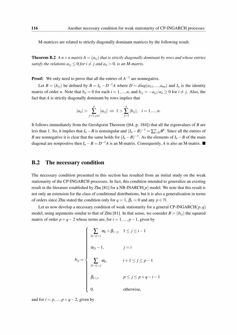
116 Another necessary condition for weak stationarity of CP-INGARCH processes
M-matrices are related to strictly diagonally dominant matrices by the following result.
Theorem B.2 A n×n matrix A = (ai j) that is strictly diagonally dominant by rows and whose entriessatisfy the relations ai j ≤ 0 for i = j and aii > 0, is an M-matrix.
Proof: We only need to prove that all the entries of A−1 are nonnegative.
Let B = (bi j) be defined by B = In −D−1A where D = diag(a11, ...,ann) and In is the identitymatrix of order n. Note that bii = 0 for each i = 1, ...,n, and bi j =−ai j/aii ≥ 0 for i = j. Also, thefact that A is strictly diagonally dominant by rows implies that
|aii|>n
∑j=1, j =i
∣∣ai j∣∣ ⇔ 1 >
n
∑j=1
|bi j|, i = 1, ...,n.
It follows immediately from the Gershgorin Theorem ([64, p. 184]) that all the eigenvalues of B areless than 1. So, it implies that In −B is nonsingular and (In −B)−1 = ∑
∞k=0 Bk. Since all the entries of
B are nonnegative it is clear that the same holds for (In −B)−1. As the elements of In −B of the maindiagonal are nonpositive then In −B = D−1A is an M-matrix. Consequently, A is also an M-matrix.
B.2 The necessary condition
The necessary condition presented in this section has resulted from an initial study on the weakstationarity of the CP-INGARCH processes. In fact, this condition intended to generalize an existingresult in the literature established by Zhu [81] for a NB-INARCH(p) model. We note that this result isnot only an extension for the class of conditional distributions, but it is also a generalization in termsof orders since Zhu stated the condition only for q = 1, β1 = 0 and any p ∈ N.
Let us now develop a necessary condition of weak stationarity for a general CP-INGARCH(p,q)model, using arguments similar to that of Zhu [81]. In that sense, we consider B = (bi j) the squaredmatrix of order p+q−2 whose terms are, for i = 1, ..., p−1, given by
bi j =
∑|k−i|= j
αk +βi− j, 1 ≤ j ≤ i−1
α2i −1, j = i
∑|k−i|= j
αk, i+1 ≤ j ≤ p−1
βi+ j, p ≤ j ≤ p+q− i−1
0, otherwise,
and for i = p, ..., p+q−2, given by
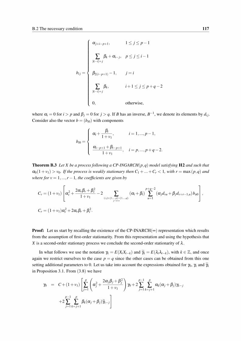
B.2 The necessary condition 117
bi j =
α j+i−p+1, 1 ≤ j ≤ p−1
∑|k−i|= j
βk +αi− j, p ≤ j ≤ i−1
β2(i−p+1)−1, j = i
∑|k−i|= j
βk, i+1 ≤ j ≤ p+q−2
0, otherwise,
where αi = 0 for i > p and β j = 0 for j > q. If B has an inverse, B−1, we denote its elements by di j.Consider also the vector b = (bi0) with components
bi0 =
αi +
βi
1+ v1, i = 1, ..., p−1,
αi−p+1 +βi−p+1
1+ v1, i = p, ..., p+q−2.
Theorem B.3 Let X be a process following a CP-INGARCH(p,q) model satisfying H2 and such thatα0(1+ v1) > v0. If the process is weakly stationary then C1 + ...+Cr < 1, with r = max(p,q) andwhere for v = 1, ...,r−1, the coefficients are given by
Cv = (1+ v1)
α2v +
2αvβv +β 2v
1+ v1−2 ∑
(i, j)∈1,...,p×1,...,q:j−i=v
(αi +βi)p+q−2
∑u=1
(α jdvu +β jdv+r−1,u)bu0
,Cr = (1+ v1)α
2r +2αrβr +β
2r .
Proof: Let us start by recalling the existence of the CP-INARCH(∞) representation which resultsfrom the assumption of first-order stationarity. From this representation and using the hypothesis thatX is a second-order stationary process we conclude the second-order stationarity of λ .
In what follows we use the notation γk = E(XtXt−k) and γk = E(λtλt−k), with k ∈ Z, and onceagain we restrict ourselves to the case p = q since the other cases can be obtained from this onesetting additional parameters to 0. Let us take into account the expressions obtained for γ0, γk and γk
in Proposition 3.1. From (3.8) we have
γ0 = C+(1+ v1)
[p
∑j=1
(α
2j +
2α jβ j +β 2j
1+ v1
)γ0 +2
p−1
∑j=1
p
∑k= j+1
αk(α j +β j)γk− j
+2p−1
∑j=1
p
∑k= j+1
βk(α j +β j)γk− j
]
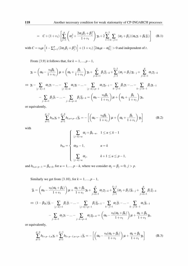
118 Another necessary condition for weak stationarity of CP-INGARCH processes
= C+(1+ v1)
[p
∑j=1
(α
2j +
2α jβ j +β 2j
1+ v1
)γ0 +2
p−1
∑v=1
∑k− j=v
(α j +β j)(αkγv +βkγv)
](B.1)
with C = v0µ
[1−∑
pj=1 (2α jβ j +β 2
j )]+(1+ v1)
[2α0µ −α2
0]> 0 and independent of t.
From (3.9) it follows that, for k = 1, ..., p−1,
γk =
(α0 −
v0βk
1+ v1
)µ +
(αk +
βk
1+ v1
)γ0 +
p
∑j=k+1
β j γ j−k +k−1
∑j=1
(α j +β j)γk− j +p
∑j=k+1
α jγ j−k
⇔ γk − ∑| j−k|=1
α jγ1− ...− ∑| j−k|=k
α jγk − ...− ∑| j−k|=p−1
α jγp−1− ∑k− j=1
β jγ1− ...− ∑k− j=k−1
β jγk−1
− ∑j−k=1
β j γ1 − ...− ∑j−k=p−k
β j γp−k =
(α0 −
v0βk
1+ v1
)µ +
(αk +
βk
1+ v1
)γ0,
or equivalently,
p−1
∑u=1
bkuγu +p−k
∑u=1
bk,u+p−1γu =−[(
α0 −v0βk
1+ v1
)µ +
(αk +
βk
1+ v1
)γ0
](B.2)
with
bku =
∑| j−k|=u
α j +βk−u, 1 ≤ u ≤ k−1
α2k −1, u = k
∑| j−k|=u
α j, k+1 ≤ u ≤ p−1,
and bk,u+p−1 = βu+k, for u = 1, ..., p− k, where we consider α j = β j = 0, j > p.
Similarly we get from (3.10), for k = 1, ..., p−1,
γk =
(α0 −
v0(αk +βk)
1+ v1
)µ +
αk +βk
1+ v1γ0 +
p
∑j=k+1
α jγ j−k +k−1
∑j=1
(α j +β j)γk− j +p
∑j=k+1
β j γ j−k
⇔ (1−β2k)γk − ∑| j−k|=1
β j γ1 − ...− ∑| j−k|=p−1
β j γp−1 − ∑k− j=1
α j γ1 − ...− ∑k− j=k−1
α j γk−1
− ∑j−k=1
α jγ1 − ...− ∑j−k=p−k
α jγp−k =
(α0 −
v0(αk +βk)
1+ v1
)µ +
αk +βk
1+ v1γ0,
or equivalently,
p−k
∑u=1
bk+p−1,uγu +p−1
∑u=1
bk+p−1,u+p−1γu =−[(
α0 −v0(αk +βk)
1+ v1
)µ +
αk +βk
1+ v1γ0
](B.3)
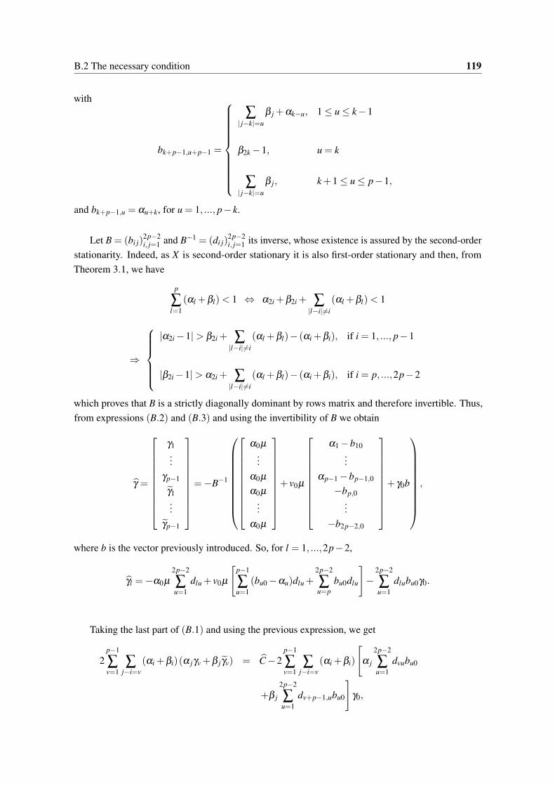
B.2 The necessary condition 119
with
bk+p−1,u+p−1 =
∑| j−k|=u
β j +αk−u, 1 ≤ u ≤ k−1
β2k −1, u = k
∑| j−k|=u
β j, k+1 ≤ u ≤ p−1,
and bk+p−1,u = αu+k, for u = 1, ..., p− k.
Let B = (bi j)2p−2i, j=1 and B−1 = (di j)
2p−2i, j=1 its inverse, whose existence is assured by the second-order
stationarity. Indeed, as X is second-order stationary it is also first-order stationary and then, fromTheorem 3.1, we have
p
∑l=1
(αl +βl)< 1 ⇔ α2i +β2i + ∑|l−i|=i
(αl +βl)< 1
⇒
|α2i −1|> β2i + ∑
|l−i|=i(αl +βl)− (αi +βi), if i = 1, ..., p−1
|β2i −1|> α2i + ∑|l−i|=i
(αl +βl)− (αi +βi), if i = p, ...,2p−2
which proves that B is a strictly diagonally dominant by rows matrix and therefore invertible. Thus,from expressions (B.2) and (B.3) and using the invertibility of B we obtain
γ =
γ1...
γp−1
γ1...
γp−1
=−B−1
α0µ
...α0µ
α0µ
...α0µ
+ v0µ
α1 −b10...
αp−1 −bp−1,0
−bp,0...
−b2p−2,0
+ γ0b
,
where b is the vector previously introduced. So, for l = 1, ...,2p−2,
γl =−α0µ
2p−2
∑u=1
dlu + v0µ
[p−1
∑u=1
(bu0 −αu)dlu +2p−2
∑u=p
bu0dlu
]−
2p−2
∑u=1
dlubu0γ0.
Taking the last part of (B.1) and using the previous expression, we get
2p−1
∑v=1
∑j−i=v
(αi +βi)(α jγv +β j γv) = C−2p−1
∑v=1
∑j−i=v
(αi +βi)
[α j
2p−2
∑u=1
dvubu0
+β j
2p−2
∑u=1
dv+p−1,ubu0
]γ0,
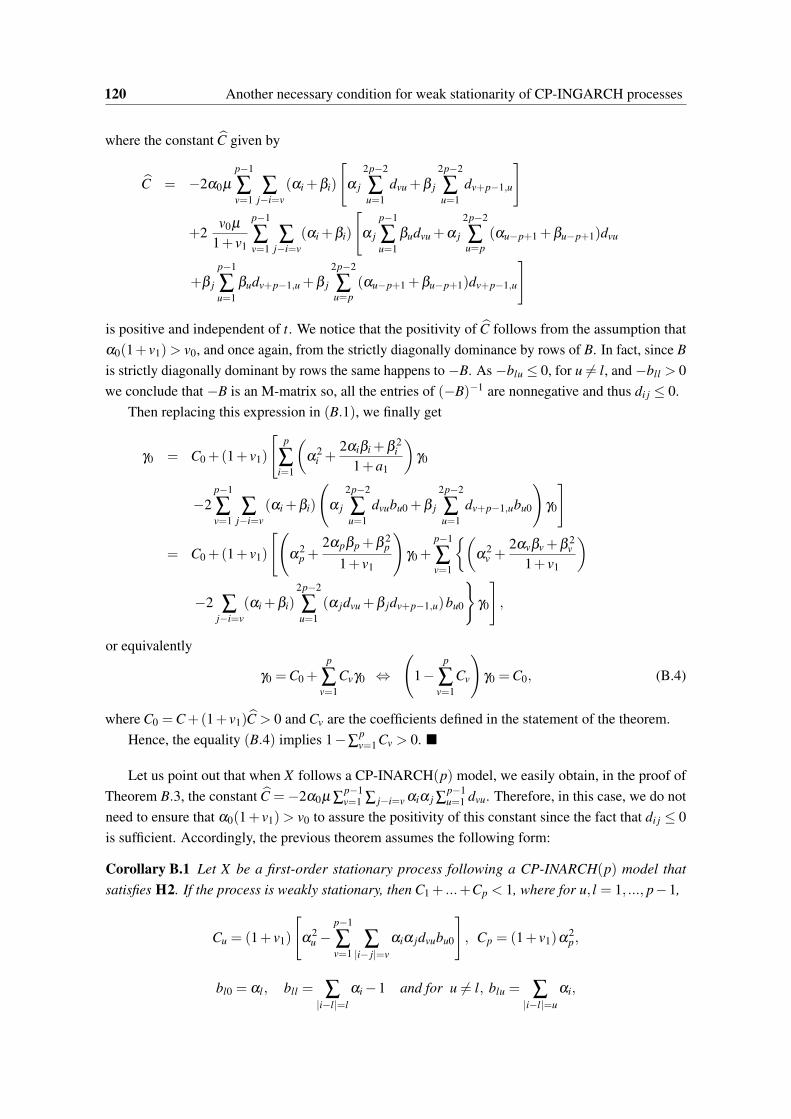
120 Another necessary condition for weak stationarity of CP-INGARCH processes
where the constant C given by
C = −2α0µ
p−1
∑v=1
∑j−i=v
(αi +βi)
[α j
2p−2
∑u=1
dvu +β j
2p−2
∑u=1
dv+p−1,u
]
+2v0µ
1+ v1
p−1
∑v=1
∑j−i=v
(αi +βi)
[α j
p−1
∑u=1
βudvu +α j
2p−2
∑u=p
(αu−p+1 +βu−p+1)dvu
+β j
p−1
∑u=1
βudv+p−1,u +β j
2p−2
∑u=p
(αu−p+1 +βu−p+1)dv+p−1,u
]
is positive and independent of t. We notice that the positivity of C follows from the assumption thatα0(1+v1)> v0, and once again, from the strictly diagonally dominance by rows of B. In fact, since Bis strictly diagonally dominant by rows the same happens to −B. As −blu ≤ 0, for u = l, and −bll > 0we conclude that −B is an M-matrix so, all the entries of (−B)−1 are nonnegative and thus di j ≤ 0.
Then replacing this expression in (B.1), we finally get
γ0 = C0 +(1+ v1)
[p
∑i=1
(α
2i +
2αiβi +β 2i
1+a1
)γ0
−2p−1
∑v=1
∑j−i=v
(αi +βi)
(α j
2p−2
∑u=1
dvubu0 +β j
2p−2
∑u=1
dv+p−1,ubu0
)γ0
]
= C0 +(1+ v1)
[(α
2p +
2αpβp +β 2p
1+ v1
)γ0 +
p−1
∑v=1
(α
2v +
2αvβv +β 2v
1+ v1
)
−2 ∑j−i=v
(αi +βi)2p−2
∑u=1
(α jdvu +β jdv+p−1,u)bu0
γ0
],
or equivalently
γ0 =C0 +p
∑v=1
Cvγ0 ⇔
(1−
p
∑v=1
Cv
)γ0 =C0, (B.4)
where C0 =C+(1+ v1)C > 0 and Cv are the coefficients defined in the statement of the theorem.Hence, the equality (B.4) implies 1−∑
pv=1Cv > 0.
Let us point out that when X follows a CP-INARCH(p) model, we easily obtain, in the proof ofTheorem B.3, the constant C =−2α0µ ∑
p−1v=1 ∑ j−i=v αiα j ∑
p−1u=1 dvu. Therefore, in this case, we do not
need to ensure that α0(1+ v1)> v0 to assure the positivity of this constant since the fact that di j ≤ 0is sufficient. Accordingly, the previous theorem assumes the following form:
Corollary B.1 Let X be a first-order stationary process following a CP-INARCH(p) model thatsatisfies H2. If the process is weakly stationary, then C1 + ...+Cp < 1, where for u, l = 1, ..., p−1,
Cu = (1+ v1)
[α
2u −
p−1
∑v=1
∑|i− j|=v
αiα jdvubu0
], Cp = (1+ v1)α
2p,
bl0 = αl, bll = ∑|i−l|=l
αi −1 and for u = l, blu = ∑|i−l|=u
αi,

B.2 The necessary condition 121
with B = (bi j) and B−1 = (di j) squared matrices of order p−1.
Remark B.1 We note that since all the entries of the matrix B−1 are nonpositive, from the previousproof, then the coefficients Cv > 0 for all v = 1, ...,r, and the necessary condition is equivalent to saythat the roots of the equation 1−C1z− ...−Crzr = 0 are outside the unit circle.
The following examples illustrate the necessary condition stated in Theorem B.3.
Example B.1 Let us consider a CP-INGARCH(2,2) model satisfying the hypothesis H2 and suchthat α1 +α2 +β1 +β2 < 1. In order to obtain the necessary condition of Theorem B.3, let us considerα0(1+ v1)> v0 and the coefficients
C1 = (α1 +β1)2 + v1α
21 −2(1+ v1)
[(α1 +β1)
2
∑u=1
(α2d1u +β2d2u)bu0
]
= (α1 +β1)2 + v1α
21 +2(1+ v1)(α1 +β1)
α2b10 +β2b20
1−α2 −β2
= (α1 +β1)2[
1+α2 +β2
1−α2 −β2
]+ v1α1
[α1(1+α2 −β2)+2α2β1
1−α2 −β2
],
C2 = (α2 +β2)2 + v1α
22 ,
since the matrices B and B−1 and the vector b are respectively given by
B =
[α2 −1 β2
α2 β2 −1
], B−1 =
[β2−1
1−α2−β2
−β21−α2−β2
−α21−α2−β2
α2−11−α2−β2
], b =
[α1 +
β11+v1
α1+β11+v1
].
Hence, the necessary condition of weak stationarity is
C1 +C2 < 1 ⇔ (α1 +β1)2(1+α2 +β2)+(α2 +β2)
[1+α2 +β2 − (α2 +β2)
2]+v1
(α
21 [1+α2 −β2]+α
22 [1−α2 −β2]+2α1α2β1
)< 1. (B.5)
Taking α2 = β2 = 0, the condition (B.5) reduces to (α1 +α2)2 + v1α2
1 < 1. So, this necessarycondition of weak stationarity of the CP-INGARCH(1,1) model equals the condition stated in Example3.1. The same happens in the CP-INGARCH(2,2) where α1 = β1 = 0. In fact, from (B.5) we get
(α2 +β2)[1+α2 +β2 − (α2 +β2)
2]+ v1α22 (1−α2 −β2)< 1 ⇔ (α2 +β2)
2 + v1α22 < 1.
Example B.2 Let us now consider a CP-INARCH(3) model satisfying the hypothesis H2 and suchthat α1 +α2 +α3 < 1. To obtain the necessary condition we analyze the coefficients
C1 = (1+ v1)
[α
21 − ∑
|i− j|=1αiα jd11b10 − ∑
|i− j|=2αiα jd21b10
]= (1+ v1)[α
21 −2(α1α2d11 +α2α3d11 +α1α3d21)b10]
= (1+ v1)
[α
21 +2
α21 α2 +α1α2α3 +α2
1 α23 +α3
1 α3
1−α2 −α1α3 −α23
],

122 Another necessary condition for weak stationarity of CP-INGARCH processes
C2 = (1+ v1)
[α
22 − ∑
|i− j|=1αiα jd12b20 − ∑
|i− j|=2αiα jd22b20
]= (1+ v1)[α
22 −2(α1α2d12 +α2α3d12 +α1α3d22)b20]
= (1+ v1)
[α
22 +2
α22 α2
3 +α1α2α3
1−α2 −α1α3 −α23
],
C3 = (1+ v1)α23 ,
as the matrices B and B−1 and the vector b are respectively given by
B =
[α2 −1 α3
α1 +α3 −1
], B−1 =
−11−α2−α1α3−α2
3
−α31−α2−α1α3−α2
3−(α1+α3)
1−α2−α1α3−α23
α2−11−α2−α1α3−α2
3
, b =
[α1
α2
].
Finally, the necessary condition of weak stationarity is
C1 +C2 +C3 < 1 ⇔ (1+ v1)[(α2
1 +α22 +α
23 )(1−α2 −α1α3 −α
23 )+2α
21 α2 +2α1α2α3
+2α21 α
23 +2α
31 α3 +2α
22 α
23 +2α1α2α3
]< 1−α2 −α1α3 −α
23 ,
We finish this Appendix saying that we are strongly convinced that the necessary condition ofweakly stationarity stated in Theorem B.3 is also a sufficient one and consequently it is equivalent tothe condition of Theorem 3.2, as we observe in the cases developed in example B.1.

Appendix C
Auxiliary Results
C.1 Lemma 3.1
In Lemma 3.1 we state that for k ∈ N0 and m ∈ N, the m-th derivative of the function ϕkt = ∏
kj=1 ϕt is
given by (ϕ
kt
)(m)(u) =
m−1
∑n=max0,m−k
k!(k−m+n)!
ϕk−m+nt (u) ×
∑k1+...+km=m−n
k1+2k2+...+mkm=mkr∈N0
(m;k1, ...,km)[ϕ′t (u)
]k1 ...[ϕ(m)t (u)]km , u ∈ R,
where(m;k1, ...,km) =
m!(1!)k1k1!(2!)k2k2! . . .(m!)kmkm!
.
Let us prove this result by induction with respect to m. Without loss of generality, let us considerm ≥ j. For m = 1 the result is valid since
(ϕk
t)′(u) = kϕ
k−1t (u)ϕ ′
t (u), u ∈ R. Now, let us assume thatthe formula is also valid for an arbitrarily fixed value of m and let us prove that it holds for m+1.
We have
(ϕ
kt
)(m+1)(u) =
ddu
m−1
∑n=m−k
k! ϕk−m+nt (u)
(k−m+n)! ∑k1+...+km=m−nk1+...+mkm=m
(m;k1, ...,km)[ϕ′t (u)
]k1 ...[ϕ(m)t (u)]km
=
m−1
∑n=m−k+1
k!( j−m+n)(k−m+n)!
ϕk−m+n−1t (u) ∑
k1+...+km=m−nk1+...+mkm=m
(m;k1, ...,km)[ϕ′t (u)
]k1+1 [ϕ′′t (u)
]k2 ...[ϕ(m)t (u)]km
+m−1
∑n=m−k
k! ϕk−m+nt (u)
(k−m+n)!
∑k1+...+km=m−nk1+...+mkm=m
k1(m;k1, ...,km)[ϕ′t (u)
]k1−1 [ϕ′′t (u)
]k2+1. . . [ϕ
(m)t (u)]km
+ ∑k1+...+km=m−nk1+...+mkm=m
k2(m;k1, ...,km)[ϕ′t (u)
]k1[ϕ′′t (u)
]k2−1 [ϕ′′′t (u)
]k3+1[ϕ
(iv)t (u)]k4 . . . [ϕ
(m)t (u)]km
123

124 Auxiliary Results
+ . . . + ∑k1+...+km=m−nk1+...+mkm=m
km(m;k1, ...,km)[ϕ′t (u)
]k1 . . . [ϕ(m)t (u)]km−1
ϕ(m+1)t (u)
=m−1
∑n=m−k+1
k! ϕk−m+n−1t (u)
(k−m+n−1)!
∑k1+...+km=m−nk1+...+mkm=m
(m;k1, ...,km)[ϕ′t (u)
]k1+1 [ϕ′′t (u)
]k2 . . . [ϕ(m)t (u)]km
+ ∑k1+...+km=m−n+1
k1+...+mkm=m
k1(m;k1, ...,km)[ϕ′t (u)
]k1−1 [ϕ′′t (u)
]k2+1 [ϕ′′′t (u)
]k3 . . . [ϕ(m)t (u)]km
+ ∑k1+...+km=m−n+1
k1+...+lkm=m
k2(m;k1, ...,km)[ϕ′t (u)
]k1[ϕ′′t (u)
]k2−1 [ϕ′′′t (u)
]k3+1[ϕ
(iv)t (u)]k4 . . . [ϕ
(m)t (u)]km
+ . . . + ∑k1+...+km=m−n+1
k1+...+mkm=m
km(m;k1, ...,km)[ϕ′t (u)
]k1 . . . [ϕ(m)t (u)]km−1
ϕ(m+1)t (u)
+k ϕ
k−1t (u)ϕ(m+1)
t (u),
where this last term results from taking n = m−1 in the summation ∑m−1n=m−k, since in this case we have
k1 + ...+ km = 1 and k1 +2k2 + ...+mkm = m which just occurs if k1 = ...= km−1 = 0 and km = 1.
Therefore,
(ϕ
kt
)(m+1)(u)=
m−1
∑n=m−k+1
k! ϕk−m+n−1t (u)
(k−m+n−1)!
∑c1+...+cm=m+1−nc1+...+mcm=m+1
(m;c1 −1,c2, ...,cm)[ϕ′t (u)
]c1 . . . [ϕ(m)t (u)]cm
+ ∑c1+...+cm=m+1−nc1+...+mcm=m+1
(c1 +1) (m;c1 +1,c2 −1,c3, ...,cm)[ϕ′t (u)
]c1 . . . [ϕ(m)t (u)]cm
+ ∑c1+...+cm=m+1−nc1+...+mcm=m+1
(c2 +1) (m;c1,c2 +1,c3 −1,c4, ...,cm)[ϕ′t (u)
]c1 . . . [ϕ(m)t (u)]cm
+ . . . + ∑c1+...+cm+1=m+1−n
c1+...+(m+1)cm+1=m+1
(cm +1) (m;c1, ...,cm−1,cm +1)[ϕ′t (u)
]c1 . . . [ϕ(m)t (u)]cmϕ
(m+1)t (u)
+ k ϕ
k−1t (u)ϕ(m+1)
t (u)
=m−1
∑n=m−k+1
k! ϕk−m+n−1t (u)
(k−m+n−1)!
∑c1+...+cm=m+1−nc1+...+mcm=m+1
(m+1;c1, ...,cm,0)[ϕ′t (u)
]c1 . . . [ϕ(m)t (u)]cm
+ ∑c1+...+cm=m+1−nc1+...+mcm=m+1
(m+1;c1, ...,cm,1)[ϕ′t (u)
]c1 . . . [ϕ(m)t (u)]cmϕ
(m+1)t (u)
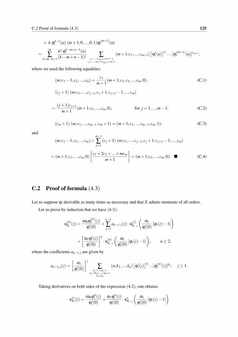
C.2 Proof of formula (4.3) 125
+ k ϕk−1t (u) (m+1;0, ...,0,1)ϕ(m+1)
t (u)
=m
∑n=m−k+1
k! ϕk−m+n−1t (u)
(k−m+n−1)! ∑c1+...+cm+1=m+1−n
c1+...+(m+1)cm+1=m+1
(m+1;c1, ...,cm+1)[ϕ′t (u)
]c1 . . . [ϕ(m+1)t (u)]cm+1 ,
where we used the following equalities:
(m;c1 −1,c2, ...,cm) =c1
m+1(m+1;c1,c2, ...,cm,0), (C.1)
(c j +1) (m;c1, ...,c j−1,c j +1,c j+1 −1, ...,cm)
=( j+1)c j+1
m+1(m+1;c1, ...,cm,0), for j = 1, ...,m−1, (C.2)
(cm +1) (m;c1, ...,cm−1,cm +1) = (m+1;c1, ...,cm−1,cm,1), (C.3)
and
(m;c1 −1,c2, ...,cm)+m−1
∑j=1
(c j +1) (m;c1, ...,c j−1,c j +1,c j+1 −1, ...,cm)
= (m+1;c1, ...,cm,0)[
c1 +2c2 + ...+mcm
m+1
]= (m+1;c1, ...,cm,0). (C.4)
C.2 Proof of formula (4.3)
Let us suppose ϕt derivable as many times as necessary and that X admits moments of all orders.
Let us prove by induction that we have (4.3):
κ(n)Xt
(z) =iα0ϕ
(n)t (z)
ϕ ′t (0)
+n−1
∑j=1
an−1, j(z) ·κ( j)Xt−1
(α1
ϕ ′t (0)
[ϕt(z)−1])
+
[α1ϕ ′
t (z)ϕ ′
t (0)
]n
·κ(n)Xt−1
(α1
ϕ ′t (0)
[ϕt(z)−1]), n ≥ 2,
where the coefficients an−1, j are given by
an−1, j(z) =[
α1
ϕ ′t (0)
] j
∑k1+...+kn= j
k1+2k2+...+nkn=nkr∈N0
(n;k1, ...,kn)[ϕ′t (z)]k1 ...[ϕ
(n)t (z)]kn , j ≥ 1.
Taking derivatives on both sides of the expression (4.2), one obtains
κ′′Xt(z) =
iα0ϕ ′′t (z)
ϕ ′t (0)
+α1ϕ ′′
t (z)ϕ ′
t (0)·κ ′
Xt−1
(α1
ϕ ′t (0)
[ϕt(z)−1])

126 Auxiliary Results
+
[α1ϕ ′
t (z)ϕ ′
t (0)
]2
·κ ′′Xt−1
(α1
ϕ ′t (0)
[ϕt(z)−1]),
so, (4.3) is valid for n = 2 since a11(z) =α1ϕ ′′
t (z)ϕ ′
t (0). Now, we assume that formula (4.3) is true for an
arbitrarily fixed integer n, n ≥ 2. Considering that an−1,0(z) = 0, it then follows that
κ(n+1)Xt
(z) =ddz
(iα0ϕ
(n)t (z)
ϕ ′t (0)
+n−1
∑j=1
an−1, j(z) ·κ( j)Xt−1
(α1
ϕ ′t (0)
[ϕt(z)−1])
+
[α1ϕ ′
t (z)ϕ ′
t (0)
]n
·κ(n)Xt−1
(α1
ϕ ′t (0)
[ϕt(z)−1]))
=iα0ϕ
(n+1)t (z)
ϕ ′t (0)
+n
∑j=1
an−1, j−1(z)α1ϕ ′
t (z)ϕ ′
t (0)·κ( j)
Xt−1
(α1
ϕ ′t (0)
[ϕt(z)−1])
+n−1
∑j=1
(α1
ϕ ′t (0)
) j
∑k1+...+kn= j
k1+...+nkn=n
k1(n;k1, ...,kn)[ϕ′t (z)]k1−1 [
ϕ′′t (z)
]k2+1. . . [ϕ
(n)t (z)]kn
+ ∑k1+...+kn= j
k1+...+nkn=n
k2(n;k1, ...,kn)[ϕ′t (z)]k1[ϕ′′t (z)
]k2−1 [ϕ′′′t (z)
]k3+1. . . [ϕ
(n)t (z)]kn + . . .
+ ∑k1+...+kn= j
k1+...+nkn=n
kn(n;k1, ...,kn)[ϕ′t (z)]k1 . . . [ϕ
(n)t (z)]kn−1
ϕ(n+1)t (z)
·κ( j)Xt−1
(α1
ϕ ′t (0)
[ϕt(z)−1])
+ n(
α1
ϕ ′t (0)
)n [ϕ′t (z)]n−1
ϕ′′t (z) ·κ
(n)Xt−1
(α1
ϕ ′t (0)
[ϕt(z)−1])
+
[α1ϕ ′
t (z)ϕ ′
t (0)
]n+1
·κ(n+1)Xt−1
(α1
ϕ ′t (0)
[ϕt(z)−1])
=iα0ϕ
(n+1)t (z)
ϕ ′t (0)
+n−1
∑j=1
(α1
ϕ ′t (0)
) j
∑c1+...+cn= j
c1+...+ncn=n+1
c1
n+1(n+1;c1, ...,cn,0)
[ϕ′t (z)]c1 . . . [ϕ
(n)t (z)]cn
+ ∑c1+...+cn= j
c1+...+ncn=n+1
2c2
n+1(n+1;c1, ...,cn,0)
[ϕ′t (z)]c1 . . . [ϕ
(n)t (z)]cn + . . .
+ ∑c1+...+cn= j
c1+...+ncn=n+1
ncn
n+1(n+1;c1, ...,cn,0)
[ϕ′t (z)]c1 . . . [ϕ
(n)t (z)]cn
+ ∑c1+...+cn+1= jc1+...+ncn=n
(n+1;c1, ...,cn,1)[ϕ′t (z)]c1 . . . [ϕ
(n)t (z)]cnϕ
(n+1)t (z)
·κ( j)Xt−1
(α1
ϕ ′t (0)
[ϕt(z)−1])
+
(α1
ϕ ′t (0)
)n
(n+1;n−1,1,0, ...,0)[ϕ′t (z)]n−1
ϕ′′t (z) ·κ
(n)Xt−1
(α1
ϕ ′t (0)
[ϕt(z)−1])
+
[α1ϕ ′
t (z)ϕ ′
t (0)
]n+1
·κ(n+1)Xt−1
(α1
ϕ ′t (0)
[ϕt(z)−1]), (C.5)

C.2 Proof of formula (4.3) 127
since we have
an−1, j−1α1ϕ ′
t (z)ϕ ′
t (0)=
(α1
ϕ ′t (0)
) j
∑k1+...+kn= j−1k1+...+nkn=n
(n;k1, ...,kn)[ϕ′t (z)]k1+1
...[ϕ(n)t (z)]kn
=
(α1
ϕ ′t (0)
) j
∑c1+...+cn= j
c1+...+ncn=n+1
(n;c1 −1,c2, ...,cn)[ϕ′t (z)]c1 ...[ϕ
(n)t (z)]cn
=
(α1
ϕ ′t (0)
) j
∑c1+...+cn= j
c1+...+ncn=n+1
c1
n+1(n+1;c1, ...,cn,0)
[ϕ′t (z)]c1 ...[ϕ
(n)t (z)]cn , from (C.1),
an−1,n−1α1ϕ ′
t (z)ϕ ′
t (0)+n(
α1
ϕ ′t (0)
)n
[ϕ ′t (z)]
n−1ϕ′′t (z) =
[n(n−1)
2+n][ϕ ′
t (z)]n−1
ϕ′′t (z)
= (n+1;n−1,1,0, . . . ,0),
∑k1+...+kn= j
k1+...+nkn=n
k1(n;k1, ...,kn)[ϕ′t (z)]k1−1 [
ϕ′′t (z)
]k2+1. . . [ϕ
(n)t (z)]kn
= ∑c1+...+cn= j
c1+...+ncn=n+1
(c1 +1)(n;c1 +1,c2 −1,c3, ...,cn)[ϕ′t (z)]c1[ϕ′′t (z)
]c2 . . . [ϕ(n)t (z)]cn
= ∑c1+...+cn= j
c1+...+ncn=n+1
2c2
n+1(n+1;c1, ...,cn,0)
[ϕ′t (z)]c1[ϕ′′t (z)
]c2 . . . [ϕ(n)t (z)]cn , from (C.2),
and
∑k1+...+kn= j
k1+...+nkn=n
kn(n;k1, ...,kn)[ϕ′t (z)]k1 . . . [ϕ
(n)t (z)]kn−1
ϕ(n+1)t (z)
= ∑c1+...+cn+1= j
c1+...+ncn+(n+1)=n+1
(cn +1)(n;c1, ...,cn−1,cn +1)[ϕ′t (z)]c1 . . . [ϕ
(n)t (z)]cnϕ
(n+1)t (z)
= ∑c1+...+cn+1= j
c1+...+ncn+(n+1)=n+1
(n+1;c1, ...,cn,1)[ϕ′t (z)]c1 . . . [ϕ
(n)t (z)]cnϕ
(n+1)t (z), from (C.3).
Thus, from (C.4), we can finally conclude that equality (C.5) is equivalent to
κ(n+1)Xt
(z) =iα0ϕ
(n+1)t (z)
ϕ ′t (0)
+
[α1ϕ ′
t (z)ϕ ′
t (0)
]n+1
·κ(n+1)Xt−1
(α1
ϕ ′t (0)
[ϕt(z)−1])

128 Auxiliary Results
+n
∑j=1
(α1
ϕ ′t (0)
) j
∑c1+...+cn+1= j
c1+...+(n+1)cn+1=n+1
(n+1;c1, ...,cn+1)[ϕ′t (z)]c1 . . . [ϕ
(n+1)t (z)]cn+1
× κ( j)Xt−1
(α1
ϕ ′t (0)
[ϕt(z)−1]).
C.3 Proof of Theorem 4.2
Let us recall that we have to show that if X is a first-order stationary process following a CP-INARCH(1) model such that H4 is satisfied, then
(a) For any k ≥ 0, we have
µ(k) = f2(v0αk1 +α0(1+α1)).
(b) For any l ≥ k ≥ 0, we have
µ(k, l) = [d0(1−α21 )− v2
0(1+α1 −2α21 )] f3α
l+k1
+v0(α0 + v0)
1−α1f2α
l1 + v0 f1 f2α
l−k1 + f1µ(k).
(c) For any m ≥ l ≥ k ≥ 0, we have
µ(k, l,m) = αm−l1
[(c0 −4v0d0 +3v3
0)+3v0(v20 −d0)α1 +(3v0d0 − c0)α
21
+(7v0d0 −6v30 − c0)α
31 +3v0(d0 −2v2
0)α41 +(6v3
0 −6v0d0 + c0)α51
f4α2l+k1
+2v0 +α0
1−α1f3[d0(1−α
21 )− v2
0(1+α1 −2α21 )]
α2l1
+v0
(1−α1)(1−α21 )
f2[2v0α0 +d0(1−α1)+ v2
0(2α1 −1)]
α2l−k1
+α0 f3
1−α1
d0(1−α
21 )− v2
0(1+α1 −2α21 )
α2(l−k)1 +
v0 +α0
1−α1µ(k, l)
− f2µ(k)[α0 +(v0 +α0)α1]]+ f1µ(k, l).
Proof: Let us recall the notations presented in formula (4.6) and (4.7) and take into account thefollowing conditional moments:
E(Xt |X t−1) = λt = α0 +α1Xt−1,
E(X2t |X t−1) = v0λt +λ
2t = v0(α0 +α1Xt−1)+(α0 +α1Xt−1)
2
= α21 X2
t−1 +α1(2α0 + v0)Xt−1 +α0(α0 + v0), (C.6)

C.3 Proof of Theorem 4.2 129
E(X3t |X t−1) = i Φ
′′′Xt |X t−1
(0) = d0λt +3v0λ2t +λ
3t (1)
= d0(α0 +α1Xt−1)+3v0(α20 +2α0α1Xt−1 +α
21 X2
t−1)+α30
+3α20 α1Xt−1 +3α0α
21 X2
t−1 +α31 X3
t−1
= α31 X3
t−1 +3α21 (v0 +α0)X2
t−1 +α1(3α20 +6v0α0 +d0)Xt−1
+α0(d0 +3v0α0 +α20 ). (C.7)
(a) Using the fact that V (Xt) = f2 and that the autocovariance function, according to Corollary 3.2,equals Γ(k) = αk
1 f2 we get
µ(k) = E(XtXt+k) =Cov(Xt ,Xt+k)+E(Xt)2 = v0α
k1 f2 +µ
2
= f2(v0αk1 +α0(1+α1)). (C.8)
(b) To derive an explicit expression for µ(k, l), 0 ≤ k ≤ l, we distinguish the following three cases:
Case 1: l > k. We have
µ(k, l) = E(XtXt+kXt+l) = E[XtXt+kE(Xt+l|X t+l−1)]
= α0E(XtXt+k)+α1E(XtXt+kXt+l−1)
= α0µ(k)+α1µ(k, l −1)
= α0µ(k)+α1[α0µ(k)+α1µ(k, l −2)]
= α0µ(k)(1+α1)+α21 µ(k, l −2)
= . . . = α0µ(k)l−k−1
∑j=0
αj
1 +αl−k1 µ(k,k)
= α0µ(k)1−α
l−k1
1−α1+α
l−k1 µ(k,k)
= αl−k1 [µ(k,k)− f1µ(k)]+ f1µ(k).
Case 2: l = k > 0. We have
µ(k,k) = E[XtE(X2t+k|X t+k−1)]
= α21 E(XtX2
t+k−1)+α1(2α0 + v0)E(XtXt+k−1)+α0(α0 + v0)E(Xt)
= α21 µ(k−1,k−1)+α1(2α0 + v0)µ(k−1)+α0(α0 + v0) f1
= α21 µ(k−1,k−1)+ v0(2α0 + v0) f2α
k1 + f1[α1(2α0 + v0) f1 +α0(α0 + v0)]
= α21 µ(k−1,k−1)+ v0(2α0 + v0) f2α
k1
+ f1[α1(2α0 + v0) f1 + f1(1−α1)(α0 + v0)]
= α21 µ(k−1,k−1)+ v0(2α0 + v0) f2α
k1 + f1µ(0)(1−α
21 )
1We note that
Φ′′′Xt |X t−1
(u) =
[iϕ ′′′
t (u)λt
ϕ ′t (0)
−3(
λt
ϕ ′t (0)
)2ϕ′t (u)ϕ
′′t (u)− i
(ϕ ′
t (u)λt
ϕ ′t (0)
)3]
exp
iλt
ϕ ′t (0)
[ϕt(u)−1], u ∈ R.
130 Auxiliary Results
= . . . = α2k1 µ(0,0)+ v0(2α0 + v0) f2
k−1
∑j=0
αk+ j1 + f1µ(0)(1−α
21 )
k−1
∑j=0
α2 j1
= α2k1 µ(0,0)+ v0(2α0 + v0) f2α
k1
1−αk1
1−α1+ f1µ(0)
= α2k1
[µ(0,0)− v0(2α0 + v0)
1−α1f2 − f1µ(0)
]+
v0(2α0 + v0)
1−α1f2α
k1 + f1µ(0).
Case 3: l = k = 0. According to the relations between the moments and the cumulants (e.g.,formula (15.10.4) in [15, p. 186]) and Theorem 4.1, we have
µ(0,0) = E(X3t ) = κ3 +3κ2µ +µ
3 = f3[d0(1−α21 )+3v2
0α21 ]+3v0 f2 f1 + f 3
1
= [d0(1−α21 )+3v2
0α21 ] f3 +
3α0v0
1−α1f2 +α
20
1+α1
1−α1f2
= [d0(1−α21 )+3v2
0α21 ] f3 +
2α0v0
1−α1f2 +
α0(v0 +α0(1+α1))
1−α1f2
= [d0(1−α21 )+3v2
0α21 ] f3 +
2α0v0
1−α1f2 + f1µ(0),
since f1 = (1−α21 ) f2.
So the above formula for µ(k,k) simplifies to
µ(k,k) = α2k1
[[d0(1−α
21 )+3v2
0α21 ] f3 −
v20
1−α1f2
]+
v0(2α0 + v0)
1−α1f2α
k1 + f1µ(0)
= α2k1
[[d0(1−α
21 )+3v2
0α21 ] f3 −
v20
1−α1f3(1−α
31 )
]+
v0(2α0 + v0)
1−α1f2α
k1 + f1µ(0)
= α2k1 f3
[d0(1−α
21 )− v2
0(1+α1 −2α21 )]+
v0(2α0 + v0)
1−α1f2α
k1 + f1µ(0),
which also holds for k = 0. Replacing this expression in µ(k, l) above, it follows that
µ(k, l) = αl−k1 [µ(k,k)− f1µ(k)]+ f1µ(k)
= αl−k1
[[d0(1−α
21 )− v2
0(1+α1 −2α21 )] f3α
2k1 +
v0(2α0 + v0)
1−α1f2α
k1
+ f1µ(0)− f1µ(k)]+ f1µ(k).
As
f1µ(0)− f1µ(k) = f1 f2(v0 +α0(1+α1))− f1[v0αk1 +α0(1+α1)] f2
= v0 f1 f2 −v0α0
1−α1f2α
k1 ,
we finally obtain, for any 0 ≤ k ≤ l,
µ(k, l) = αl−k1
[[d0(1−α
21 )− v2
0(1+α1 −2α21 )] f3α
2k1 +
v0(α0 + v0)
1−α1f2α
k1 + v0 f1 f2
]+ f1µ(k)
= [d0(1−α21 )− v2
0(1+α1 −2α21 )] f3α
l+k1 +
v0(α0 + v0)
1−α1f2α
l1 + v0 f1 f2α
l−k1 + f1µ(k).

C.3 Proof of Theorem 4.2 131
(c) In what concerns the fourth-order moments µ(k, l,m) with 0 ≤ k ≤ l ≤ m, we proceed in a similarway as above and distinguish the following four cases:
Case 1: m > l. As above we have
µ(k, l,m) = E(XtXt+kXt+lXt+m) = E[XtXt+kXt+lE(Xt+m|X t+m−1)]
= α0E(XtXt+kXt+l)+α1E(XtXt+kXt+lXt+m−1)
= α0µ(k, l)+α1µ(k, l,m−1)
= . . . = αm−l1 [µ(k, l, l)− f1µ(k, l)]+ f1µ(k, l).
Case 2: m = l > k. For this case, using formula (C.6), we obtain
µ(k, l, l) = E[XtXt+kE(X2t+l|X t+l−1)]
= α21 µ(k, l −1, l −1)+α1(v0 +2α0)µ(k, l −1)+α0(v0 +α0)µ(k)
= α21 µ(k, l −1, l −1)+α0(v0 +α0)µ(k)
+α1(v0 +2α0)[d0(1−α
21 )− v2
0(1+α1 −2α21 )] f3α
l−1+k1
+v0(α0 + v0)
1−α1f2α
l−11 + v0 f1 f2α
l−1−k1 + f1µ(k)
,
by replacing µ(k, l −1). So,
µ(k, l, l) = α21 µ(k, l −1, l −1)+ f1µ(k) [α1(v0 +2α0)+(1−α1)(v0 +α0)]
+αl1(v0 +2α0)
[d0(1−α
21 )− v2
0(1+α1 −2α21 )] f3α
k1
+v0(α0 + v0)
1−α1f2 + v0 f1 f2α
−k1
= . . . = α
2(l−k)1 µ(k,k,k)+ f1µ(k)(v0 +α0(1+α1))
l−k−1
∑j=0
α2 j1
+(v0 +2α0)[d0(1−α
21 )− v2
0(1+α1 −2α21 )] f3α
k1
+v0(α0 + v0)
1−α1f2 + v0 f1 f2α
−k1
l−k−1
∑j=0
αl+ j1
= α2(l−k)1 µ(k,k,k)+µ(k)(v0 +α0(1+α1)) f2(1−α
2(l−k)1 )
+v0 +2α0
1−α1
[d0(1−α
21 )− v2
0(1+α1 −2α21 )] f3α
k1
+v0(α0 + v0)
1−α1f2 + v0 f1 f2α
−k1
(α l
1 −α2l−k1 ).
Since µ(0) = (v0 +α0(1+α1)) f2 and replacing µ(k), we get
µ(k, l, l) = α2(l−k)1 µ(k,k,k)+µ(k)µ(0)− f2(v0α
k1 +α0(1+α1))µ(0)α
2(l−k)1
+v0 +2α0
1−α1
[d0(1−α
21 )− v2
0(1+α1 −2α21 )] f3α
l+k1
+v0(α0 + v0)
1−α1f2α
l1 + v0 f1 f2α
l−k1

132 Auxiliary Results
−v0 +2α0
1−α1
[d0(1−α
21 )− v2
0(1+α1 −2α21 )]
f3α2l1
−(v0 +2α0)v0(v0 +α0)
(1−α1)2 f2α2l−k1 − v0(v0 +2α0)
1−α1f1 f2α
2(l−k)1
= α2(l−k)1 µ(k,k,k)+µ(k)µ(0)
− f2v0
[f2(v0 +α0(1+α1))+
(v0 +2α0)(v0 +α0)
(1−α1)2
]α
2l−k1
− f1
[f1µ(0)+
v0(v0 +2α0)
1−α1f2
]α
2(l−k)1 +
v0 +2α0
1−α1[µ(k, l)− f1µ(k)]
−v0 +2α0
1−α1
[d0(1−α
21 )− v2
0(1+α1 −2α21 )]
f3α2l1 .
So, replacing µ(0), recalling µ(0,0) and taking into account that f11−α1
= (1+α1) f2, we get
µ(k, l, l) = α2(l−k)1 µ(k,k,k)+µ(k) f2[v0 +α0(1+α1)]
− f2v0
(1−α1)(1−α21 )
[v2
0(1+α1)+ v0α0(4+3α1)+3α20 (1+α1)
]α
2l−k1
− f1
µ(0,0)− [d0(1−α
21 )+3v2
0α21 ] f3 +
v20 f2
1−α1
α
2(l−k)1
+v0 +2α0
1−α1µ(k, l)− (v0 +2α0)(1+α1) f2µ(k)
−v0 +2α0
1−α1
[d0(1−α
21 )− v2
0(1+α1 −2α21 )]
f3α2l1
= α2(l−k)1 µ(k,k,k)−µ(k) f2[α0 +(v0 +α0)α1]
− f2v0
(1−α1)(1−α21 )
[v2
0(1+α1)+ v0α0(4+3α1)+3α20 (1+α1)
]α
2l−k1
− f1
µ(0,0)− [d0(1−α
21 )+3v2
0α21 ] f3 +
v20 f2
1−α1
α
2(l−k)1
+v0 +2α0
1−α1µ(k, l)− v0 +2α0
1−α1
[d0(1−α
21 )− v2
0(1+α1 −2α21 )]
f3α2l1 . (C.9)
Case 3: m = l = k > 0. From formula (C.7) we have
µ(k,k,k) = E[XtE(X3t+k|X t+k−1)]
= α31 µ(k−1,k−1,k−1)+3α
21 (v0 +α0)µ(k−1,k−1)
+α1(d0 +6v0α0 +3α20 )µ(k−1)+α0(d0 +3v0α0 +α
20 )µ.
Replacing µ(k−1,k−1) and thereafter µ(k−1), we deduce
µ(k,k,k) = α31 µ(k−1,k−1,k−1)
+3α21 (v0 +α0)
[d0(1−α
21 )− v2
0(1+α1 −2α21 )] f3α
2k−21
+v0(α0 + v0)
1−α1f2α
k−11 + v0 f1 f2 + f1µ(k−1)
+α1(d0 +6v0α0 +3α
20 )µ(k−1)+α0(d0 +3v0α0 +α
20 )µ
= α31 µ(k−1,k−1,k−1)
C.3 Proof of Theorem 4.2 133
+3(v0 +α0)[d0(1−α
21 )− v2
0(1+α1 −2α21 )]
f3α2k1 +3α1
v0(v0 +α0)2
1−α1f2α
k1
+3α21 (v0 +α0)
v0 f1 f2 + f1 f2(v0α
k−11 +α0(1+α1))
+(d0 +6v0α0 +3α
20 ) f2
[v0α
k1 +α0α1(1+α1)
]+α0(d0 +3v0α0 +α
20 ) f1
= α31 µ(k−1,k−1,k−1)
+3(v0 +α0)[d0(1−α
21 )− v2
0(1+α1 −2α21 )]
f3α2k1
+v0 f2
1−α1
[3α1(v0 +α0)
2 +3α1(v0 +α0)α0 +(d0 +6v0α0 +3α20 )(1−α1)
]α
k1
+ f1 f2
3α21 (v0 +α0)(v0 +α0(1+α1))+(d0 +6v0α0 +3α
20 )α1(1−α1)(1+α1)
+(d0 +3v0α0 +α20 )(1−α1)(1−α
21 ).
Making some calculations and then recalling the expression of µ(0,0), we obtain
µ(k,k,k) = α31 µ(k−1,k−1,k−1)
+3(v0 +α0)[d0(1−α
21 )− v2
0(1+α1 −2α21 )]
f3α2k1
+v0 f2
1−α1
[3α
20 (1+α1)+3v0α0(2+α1)+d0(1−α1)+3v2
0α1]
αk1
+ f1 f2
d0(1−α
21 )+3v2
0α21 +
3v0α0
1−α1(1−α
31 )+
α20 (1+α1)
1−α1(1−α
31 )
= α
31 µ(k−1,k−1,k−1)
+3(v0 +α0)[d0(1−α
21 )− v2
0(1+α1 −2α21 )]
f3α2k1
+v0 f2
1−α1
[3α
20 (1+α1)+3v0α0(2+α1)+d0(1−α1)+3v2
0α1]
αk1
+ f1(1−α31 )µ(0,0).
Replacing successively the expression of µ(k− j,k− j,k− j), j = 1, ...,k−1, it remains
µ(k,k,k) = α3k1 µ(0,0,0)+3(v0 +α0)
[d0(1−α
21 )− v2
0(1+α1 −2α21 )]
f3
k−1
∑j=0
α2k+ j1
+v0 f2
1−α1
[3α
20 (1+α1)+3v0α0(2+α1)+d0(1−α1)+3v2
0α1] k−1
∑j=0
αk+2 j1
+ f1(1−α31 )µ(0,0)
k−1
∑j=0
α3 j1
= α3k1
µ(0,0,0)−3(v0 +α0)
[d0(1−α
21 )− v2
0(1+α1 −2α21 )] f3
1−α1
− v0 f2
(1−α1)(1−α21 )
[3α
20 (1+α1)+3v0α0(2+α1)+d0(1−α1)+3v2
0α1]
− f1µ(0,0)+3(v0 +α0) f3α2k
11−α1
[d0(1−α
21 )− v2
0(1+α1 −2α21 )]
+v0 f2αk
1
(1−α1)(1−α21 )
[3α
20 (1+α1)+3v0α0(2+α1)+d0(1−α1)+3v2
0α1]
+ f1µ(0,0). (C.10)

134 Auxiliary Results
Let us now take into account that replacing µ(0,0), we obtain
3(v0 +α0)f3
1−α1
[d0(1−α
21 )− v2
0(1+α1 −2α21 )]
+v0 f2
(1−α1)(1−α21 )
[3α
20 (1+α1)+3v0α0(2+α1)+d0(1−α1)+3v2
0α1]
+ f1µ(0,0)
= 3(v0 +α0)f3
1−α1
[d0(1−α
21 )− v2
0(1+α1 −2α21 )]
+v0 f2
(1−α1)(1−α21 )
[3α
20 (1+α1)+3v0α0(2+α1)+d0(1−α1)+3v2
0α1]
+ f1 f3[d0(1−α21 )+3v2
0α21 ]+ f1 f2
2v0α0
1−α1+ f 2
1 f2(v0 +α0(1+α1))
which, highlighting f31−α2
1and noting that f2 = (1−α3
1 ) f3, equals
f3
1−α21
3(v0 +α0)(1+α1)[d0(1−α
21 )− v2
0(1+α1 −2α21 )]
+1−α3
11−α1
[3v0α20 (1+α1)+3v2
0α0(2+α1)+ v0d0(1−α1)+3v30α1]
+α0(1+α1)[d0(1−α21 )+3v2
0α21 ]+ (1+α1)
1−α31
1−α1[2v0α
20 + v0α
20 +α
30 (1+α1)]
=
f3
1−α21
4v0d0 −3v3
0 +3v0(d0 − v20)α1 +3v0(2v2
0 −d0)α21 + v0(9v2
0 −4d0)α31
+(3v2
0 +4d0 +(3v20 +4d0)α1 +(15v2
0 −4d0)α21 +(12v2
0 −4d0)α31)
α0
+6v0α20 (1+α1)(1+α1 +α
21 )+α
30 (1+α1)
2(1+α1 +α21 )
= f4
4v0d0 −3v30 +3v0(d0 − v2
0)α1 +3v0(v20 +d0)α
21
+v0(6v20 −d0)α
31 +3v0(2v2
0 −d0)α41 + v0(9v2
0 −4d0)α51
+(1+α21 )(3v2
0 +4d0 +(3v20 +4d0)α1 +(15v2
0 −4d0)α21 +(12v2
0 −4d0)α31)
α0
+6v0α20 (1+α
21 )(1+α1)(1+α1 +α
21 )+α
30 (1+α
21 )(1+α1)
2(1+α1 +α21 ),
since f31−α2
1= f4(1+α2
1 ) and developing the calculations.
So, replacing the expression above in the coefficient of α3k1 in formula (C.10), we finally get
µ(k,k,k) =
µ(0,0,0)− f4[4v0d0 −3v3
0 +3v0(d0 − v20)α1 + v0(3v2
0 +d0)α21
+v0(6v20 −d0)α
31 +3v0(2v2
0 −d0)α41 + v0(9v2
0 −4d0)α51
+α0(1+α21 )[3v2
0 +4d0 +(3v20 +4d0)α1 +(15v2
0 −4d0)α21 +(12v2
0 −4d0)α31]
+6v0α20 (1+α
21 )(1+α1)(1+α1 +α
21 )
+α30 (1+α
21 )(1+α1)
2(1+α1 +α21 )]
α3k1
+3v0 +α0
1−α1f3[d0(1−α
21 )− v2
0(1+α1 −2α21 )]
α2k1 + f1µ(0,0)
+v0
(1−α1)(1−α21 )
f2[3α
20 (1+α1)+3v0α0(2+α1)
+d0(1−α1)+3v20α1]
αk1 . (C.11)

C.3 Proof of Theorem 4.2 135
Case 4: m = l = k = 0. Once again, according to the relations between the moments and thecumulants (e.g., formula (15.10.4) in [15, p. 186]) and Theorem 4.1, we obtain
µ(0,0,0) = E(X4t ) = κ4 +3κ
22 +6κ2µ
2 +4κ3µ +µ4
= f4
c0(1−α21 )(1−α
31 )+ v3
0(3α21 +15α
51 )+ v0d0(4α
21 +6α
31 −10α
51 )
+3v20 f 2
2 +6v0 f2 f 21 +4 f3[d0(1−α
21 )+3v2
0α21 ] f1 + f 4
1
= f4
c0(1−α21 )(1−α
31 )+ v3
0(3α21 +15α
51 )+ v0d0(4α
21 +6α
31 −10α
51 )
+3v20α0
(1−α41 )(1−α3
1 )
(1−α1)(1−α21 )
+6v0α20(1−α4
1 )(1−α31 )
(1−α1)2
+4α0(1−α4
1 )
1−α1[d0(1−α
21 )+3v2
0α21 ]+α
30(1−α4
1 )(1−α31 )(1−α2
1 )
(1−α1)3
= f4
c0(1−α
21 )(1−α
31 )+ v3
0(3α21 +15α
51 )+ v0d0(4α
21 +6α
31 −10α
51 )
+3v20α0(1+α
21 )(1+α1 +α
21 )+6v0α
20 (1+α1)(1+α
21 )(1+α1 +α
21 )
+4α0(1+α1)(1+α21 )[d0(1−α
21 )+3v2
0α21 ]+α
30 (1+α1)
2(1+α21 )(1+α1 +α
21 )
= f4
c0 +(3v30 +4v0d0 − c0)α
21 +(6v0d0 − c0)α
31 +(15v3
0 −10v0d0 + c0)α51
+α0(1+α21 )[3v2
0 +4d0 +(3v20 +4d0)α1 +(15v2
0 −4d0)α21 +(12v2
0 −4d0)α31]
+6v0α20 (1+α1)(1+α
21 )(1+α1 +α
21 )+α
30 (1+α1)
2(1+α21 )(1+α1 +α
21 ).
So the formula (C.11) for µ(k,k,k) studied in case 3 simplifies to
µ(k,k,k) = f4
c0 −4v0d0 +3v30 +3v0(v2
0 −d0)α1 +(3v0d0 − c0)α21
+(7v0d0 −6v30 − c0)α
31 +3v0(d0 −2v2
0)α41 +(6v3
0 −6v0d0 + c0)α51
α3k1
+3v0 +α0
1−α1f3[d0(1−α
21 )− v2
0(1+α1 −2α21 )]
α2k1 + f1µ(0,0)
+v0
(1−α1)(1−α21 )
f2[3α
20 (1+α1)+3v0α0(2+α1)+d0(1−α1)+3v2
0α1]
αk1 .
Inserting into the formula (C.9) for µ(k, l, l) stated in case 2, we obtain
µ(k, l, l) = f4
c0 −4v0d0 +3v30 +3v0(v2
0 −d0)α1 +(3v0d0 − c0)α21
+(7v0d0 −6v30 − c0)α
31 +3v0(d0 −2v2
0)α41 +(6v3
0 −6v0d0 + c0)α51
α2l+k1
+3v0 +3α0 − v0 −2α0
1−α1f3[d0(1−α
21 )− v2
0(1+α1 −2α21 )]
α2l1
+ f1
µ(0,0)−µ(0,0)−
v20 f2
1−α1+[d0(1−α
21 )+3v2
0α21 ] f3
α
2(l−k)1
+v0
(1−α1)(1−α21 )
f2[3α
20 (1+α1)+3v0α0(2+α1)+d0(1−α1)+3v2
0α1
−v20(1+α1)− v0α0(4+3α1)−3α
20 (1+α1)
]α
2l−k1
+v0 +2α0
1−α1µ(k, l)− f2µ(k)[α0 +(v0 +α0)α1]
= f4
c0 −4v0d0 +3v30 +3v0(v2
0 −d0)α1 +(3v0d0 − c0)α21
+(7v0d0 −6v30 − c0)α
31 +3v0(d0 −2v2
0)α41 +(6v3
0 −6v0d0 + c0)α51
α2l+k1

136 Auxiliary Results
+2v0 +α0
1−α1f3[d0(1−α
21 )− v2
0(1+α1 −2α21 )]
α2l1
+
α0 f3
1−α1[d0(1−α
21 )− v2
0(1+α1 −2α21 )]
α
2(l−k)1
+v0
(1−α1)(1−α21 )
f2[2v0α0 +d0(1−α1)+ v2
0(2α1 −1)]
α2l−k1
+v0 +2α0
1−α1µ(k, l)− f2µ(k)[α0 +(v0 +α0)α1].
So it follows that we have
µ(k, l,m) = αm−l1 [µ(k, l, l)− f1µ(k, l)]+ f1µ(k, l)
= αm−l1
[f4
c0 −4v0d0 +3v30 +3v0(v2
0 −d0)α1 +(3v0d0 − c0)α21
+(7v0d0 −6v30 − c0)α
31 +3v0(d0 −2v2
0)α41 +(6v3
0 −6v0d0 + c0)α51
α2l+k1
+2v0 +α0
1−α1f3[d0(1−α
21 )− v2
0(1+α1 −2α21 )]
α2l1
+
α0 f3
1−α1[d0(1−α
21 )− v2
0(1+α1 −2α21 )]
α
2(l−k)1
+v0
(1−α1)(1−α21 )
f2[2v0α0 +d0(1−α1)+ v2
0(2α1 −1)]
α2l−k1
+v0 +α0
1−α1µ(k, l)− f2µ(k)[α0 +(v0 +α0)α1]
]+ f1µ(k, l),
which holds for all 0 ≤ k ≤ l ≤ m.
C.4 Proof of Corollary 4.2
We recall that we have to prove that if X is a first-order stationary process following a CP-INARCH(1)model such that H4 is satisfied, then
(a) For any s ≥ 0, we have
µ(s) = κ(s) = v0αs1 f2.
(b) For any l ≥ s ≥ 0, we have
µ(s, l) = κ(s, l)
= f3αl1[v
20(1+α1 +α
21 )−v2
0(1+α1 −2α21 )−d0(1−α
21 )α
s1].
(c) For any m ≥ l ≥ s ≥ 0, we have
κ(s, l,m) = αm1 f4
[c0 +3v3
0 −4v0d0 +3v0(v20 −d0)α1 +(3α0d0 − c0)α
21
+(7v0d0 −6v30 − c0)α
31 +3v0(d0 −2v2
0)α41 +(6v3
0 −6v0d0 + c0)α51
αl+s1
+v0(1+α1 +α21 +α
31 )[d0(1−α
21 )− v2
0(1+α1 −2α21 )](2α
l1 +α
s1)

C.4 Proof of Corollary 4.2 137
+v0(1+α1 +α21 )(1+α
21 )[(1+α1)v2
0 +(d0(1−α1)+ v20(2α1 −1))α l−s
1 ]],
µ(s, l,m) = κ(s, l,m)+ v20 f 2
2 αm−l+s1 +2v2
0 f 22 α
m+l−s1 .
Proof:
(a) From (4.11) and (4.8) we have, for any s ≥ 0,
µ(s) = κ(s) = Cov(Xt ,Xt+s) = v0αs1 f2.
(b) From (4.12), (4.9) and using the expressions stated in Theorem 4.2, the third-order centralmoment and cumulant of X are given by
µ(s, l) = κ(s, l)
= [d0(1−α21 )− v2
0(1+α1 −2α21 )] f3α
l+s1 +
v0(α0 + v0)
1−α1f2α
l1
+v0 f1 f2αl−s1 + f1µ(s)− f1µ(s)
− f1[ f2(v0αl−s1 +α0(1+α1))+ f2(v0α
l1 +α0(1+α1))−2 f 2
1 ]
= [d0(1−α21 )− v2
0(1+α1 −2α21 )] f3α
l+s1 +
v0(α0 + v0)
1−α1f2α
l1
+v0 f1 f2αl−s1 − f1 f2v0(α
l−s1 +α
l1)
= [d0(1−α21 )− v2
0(1+α1 −2α21 )] f3α
l+s1 +
v20 f2
1−α1α
l1
= f3αl1[v
20(1+α1 +α
21 )−v2
0(1+α1 −2α21 )−d0(1−α
21 )α
s1],
for l ≥ s ≥ 0.
(c) In what concerns the fourth-order cumulant we have from (4.10) and the expressions stated inTheorem 4.2, for m ≥ l ≥ s ≥ 0,
κ(s, l,m) = αm−l1αm−l1αm−l1
[α
2l+s1 f4
c0 −4v0d0 +3v3
0 +3v0(v20 −d0)α1 +(3v0d0 − c0)α
21
+(7v0d0 −6v30 − c0)α
31 +3v0(d0 −2v2
0)α41 +(6v3
0 −6v0d0 + c0)α51
+2v0 +α0
1−α1f3[d0(1−α
21 )− v2
0(1+α1 −2α21 )]
α2l1
+
α0 f3
1−α1[d0(1−α
21 )− v2
0(1+α1 −2α21 )]
α
2(l−s)1+
α0 f3
1−α1[d0(1−α
21 )− v2
0(1+α1 −2α21 )]
α
2(l−s)1+
α0 f3
1−α1[d0(1−α
21 )− v2
0(1+α1 −2α21 )]
α
2(l−s)1
+v0
(1−α1)(1−α21 )
f2[2v0α0 +d0(1−α1)+ v2
0(2α1 −1)]
α2l−s1
+v0 +α0
1−α1µ(s, l)− f2µ(s)[α0 +(v0 +α0)α1]
]+ f1µ(s, l)− f1µ(s, l)+ f1µ(s, l)− f1µ(s, l)+ f1µ(s, l)− f1µ(s, l)
− f1− f1− f1
([d0(1−α
21 )− v2
0(1+α1 −2α21 )] f3α
m+l−2s1[d0(1−α
21 )− v2
0(1+α1 −2α21 )] f3α
m+l−2s1[d0(1−α
21 )− v2
0(1+α1 −2α21 )] f3α
m+l−2s1 +
v0(v0 +α0)
1−α1f2α
m−s1

138 Auxiliary Results
+v0 f1 f2αm−l1 + f1µ(l − s)− f1 f2(v0α
l−s1 +α0(1+α1))+ f1µ(l − s)− f1 f2(v0αl−s1 +α0(1+α1))+ f1µ(l − s)− f1 f2(v0αl−s1 +α0(1+α1))
+[d0(1−α21 )− v2
0(1+α1 −2α21 )] f3α
m+l1
+v0(v0 +α0)
1−α1f2α
m1 + f1 f2v0α
m−l1 + f1µ(l)− f1µ(l)+ f1µ(l)− f1µ(l)+ f1µ(l)− f1µ(l)+
v0(v0 +α0)
1−α1f2α
m1
+[d0(1−α21 )− v2
0(1+α1 −2α21 )] f3α
m+s1 + v0 f1 f2α
m−s1 + f1µ(s)− f1µ(s)+ f1µ(s)− f1µ(s)+ f1µ(s)− f1µ(s)
)−( f2[v0α
s1 +α0(1+α1)]− f 2
1 )( f2[v0αm−l1 +α0(1+α1)]− f 2
1 )
−( f2[v0αl1 +α0(1+α1)]− f 2
1 )( f2[v0αm−s1 +α0(1+α1)]− f 2
1 )
−( f2[v0αm1 +α0(1+α1)]− f 2
1 )( f2[v0αl−s1 +α0(1+α1)]− f 2
1 )
+ f 21(
f2[v0αm1 +α0(1+α1)]+ f2[v0α
m−s1 +α0(1+α1)]
+ f2[v0αm−l1 +α0(1+α1)]−3 f 2
1
),
where we highlight, using bold, expressions whose sum equals zero.
So, taking into account that
− f2µ(s)[α0 +(v0 +α0)α1]αm−l1 =
[− f1
α0 + v0
1−α1µ(s)+ v0 f2µ(s)
]α
m−l1
and
−( f2[v0αs1 +α0(1+α1)]− f 2
1 )( f2[v0αm−l1 +α0(1+α1)]− f 2
1 )
−( f2[v0αl1 +α0(1+α1)]− f 2
1 )( f2[v0αm−s1 +α0(1+α1)]− f 2
1 )
−( f2[v0αm1 +α0(1+α1)]− f 2
1 )( f2[v0αl−s1 +α0(1+α1)]− f 2
1 )
+ f 21(
f2[v0αm1 +α0(1+α1)]+ f2[v0α
m−s1 +α0(1+α1)]
+ f2[v0αm−l1 +α0(1+α1)]−3 f 2
1
)= − f 2
2 (v0αs1 +α0(1+α1))(v0α
m−l1 +α0(1+α1))
+ f 21 f2(v0α
s1 +α0(1+α1))+ f 2
1 f2(v0αm−l1 +α0(1+α1))− f 4
1
− f 22 (v0α
l1 +α0(1+α1))(v0α
m−s1 +α0(1+α1))
+ f 21 f2(v0α
l1 +α0(1+α1))+ f 2
1 f2(v0αm−s1 +α0(1+α1))− f 4
1
− f 22 (v0α
m1 +α0(1+α1))(v0α
l−s1 +α0(1+α1))
+ f 21 f2(v0α
m1 +α0(1+α1))+ f 2
1 f2(v0αl−s1 +α0(1+α1))− f 4
1
+ f 21 f2(v0α
m1 +α0(1+α1))+ f 2
1 f2(v0αm−s1 +α0(1+α1))
+ f 21 f2[v0α
m−l1 +α0(1+α1)]−3 f 4
1
= − f 22
[v2
0αm−l+s1 +α0(1+α1)v0α
s1 +α0(1+α1)v0α
m−l1 +α
20 (1+α1)
2]
+ f 21 f2(v0α
s1 +α0(1+α1))+2 f 2
1 f2(v0αm−l1 +α0(1+α1))−6 f 4
1
− f 22
[v2
0αm+l−s1 +α0(1+α1)v0α
l1 +α0(1+α1)v0α
m−s1 +α
20 (1+α1)
2]
+ f 21 f2(v0α
l1 +α0(1+α1))+2 f 2
1 f2(v0αm−s1 +α0(1+α1))
− f 22
[v2
0αm+l−s1 +α0(1+α1)v0α
l−s1 +α0(1+α1)v0α
m1 +α
20 (1+α1)
2]

C.4 Proof of Corollary 4.2 139
+ f 21 f2(v0α
l−s1 +α0(1+α1))+2 f 2
1 f2(v0αm1 +α0(1+α1))
= −v20 f 2
2 αm−l+s1 +[ f 2
1 f2v0 − f 22 v0α0(1+α1)][α
s1 +α
l1 +α
l−s1 ]
+[2 f 21 f2v0 − f 2
2 v0α0(1+α1)][αm−s1 +α
m−l1 +α
m1 ]−2 f 2
2 v20α
m+l−s1
−3 f 22 α
20 (1+α1)
2 +9 f 21 f2α0(1+α1)−6 f 4
1
= −v20 f 2
2 [αm−l+s1 +2α
m+l−s1 ]+ v0 f 2
1 f2[αm−l1 +α
m−s1 +α
m1 ]
we obtain
κ(s, l,m) = αm+l+s1 f4
c0 −4v0d0 +3v3
0 +3v0(v20 −d0)α1 +(3v0d0 − c0)α
21
+(7v0d0 −6v30 − c0)α
31 +3v0(d0 −2v2
0)α41 +(6v3
0 −6v0d0 + c0)α51
+2v0 +α0α0α0
1−α11−α11−α1f3α
m+l1
[d0(1−α
21 )− v2
0(1+α1 −2α21 )]
f3αm+l1
[d0(1−α
21 )− v2
0(1+α1 −2α21 )]
f3αm+l1
[d0(1−α
21 )− v2
0(1+α1 −2α21 )]
+v0
(1−α1)(1−α21 )
f2αm+l−s1+
v0
(1−α1)(1−α21 )
f2αm+l−s1+
v0
(1−α1)(1−α21 )
f2αm+l−s1
[2v0α02v0α02v0α0 +d0(1−α1)+ v2
0(2α1 −1)]
+v0 +α0
1−α1α
m−l1 µ(s, l)− f1µ(s)+ v0 f2µ(s)αm−l
1
− f1− f1− f1
(v0(v0 +2α0)
1−α1f2α
m−s1 +
2v0(v0 +α0)
1−α1f2α
m1 +2v0 f1 f2α
m−l1
+[d0(1−α21 )− v2
0(1+α1 −2α21 )] f3+[d0(1−α
21 )− v2
0(1+α1 −2α21 )] f3+[d0(1−α
21 )− v2
0(1+α1 −2α21 )] f3[α
m+l1αm+l1αm+l1 +α
m+s1 ]
)−v2
0 f 22−v2
0 f 22−v2
0 f 22 (α
m−l+s1 +2α
m+l−s12αm+l−s12αm+l−s1 )+ v0 f 2
1 f2(αm1 +α
m−s1 +α
m−l1 ).
As the sum of the expressions in bold equals 0 and replacing µ(s, l), we obtain
κ(s, l,m) = αm+l+s1 f4
c0 −4v0d0 +3v3
0 +3v0(v20 −d0)α1 +(3v0d0 − c0)α
21
+(7v0d0 −6v30 − c0)α
31 +3v0(d0 −2v2
0)α41 +(6v3
0 −6v0d0 + c0)α51
+2v0
1−α1f3α
m+l1
[d0(1−α
21 )− v2
0(1+α1 −2α21 )]
+v0
(1−α1)(1−α21 )
f2αm+l−s1
[d0(1−α1)+ v2
0(2α1 −1)]
+v0 +α0α0α0
1−α11−α11−α1α
m−l1αm−l1αm−l1
[d0(1−α
21 )− v2
0(1+α1 −2α21 )] f3α
l+s1d0(1−α
21 )− v2
0(1+α1 −2α21 )] f3α
l+s1d0(1−α
21 )− v2
0(1+α1 −2α21 )] f3α
l+s1
+v0(v0 +α0)
1−α1f2α
l1 + v0 f1 f2α
l−s1
− f1− f1− f1
(v0(v0 +2α0)
1−α1f2α
m−s1 +[d0(1−α
21 )− v2
0(1+α1 −2α21 )] f3α
m+s1[d0(1−α
21 )− v2
0(1+α1 −2α21 )] f3α
m+s1[d0(1−α
21 )− v2
0(1+α1 −2α21 )] f3α
m+s1
−v0 f1 f2αm1 +
2v0(v0 +α0)
1−α1f2α
m1 − v0 f1 f2α
m−s1
)+v0 f2α
m−l1 [µ(s)− f 2
1 ]− v20 f 2
2 αm−l+s1+v0 f2α
m−l1 [µ(s)− f 2
1 ]− v20 f 2
2 αm−l+s1+v0 f2α
m−l1 [µ(s)− f 2
1 ]− v20 f 2
2 αm−l+s1 .
The sum of the expressions in bold equals 0 and then we conclude

140 Auxiliary Results
κ(s, l,m) = αm+l+s1 f4
c0 −4v0d0 +3v3
0 +3v0(v20 −d0)α1 +(3v0d0 − c0)α
21
+(7v0d0 −6v30 − c0)α
31 +3v0(d0 −2v2
0)α41 +(6v3
0 −6v0d0 + c0)α51
+2v0
1−α1f3α
m+l1
d0(1−α
21 )− v2
0(1+α1 −2α21 )
+v0
(1−α1)(1−α21 )
f2αm+l−s1
d0(1−α1)+ v2
0(2α1 −1)
+v0 +α0
1−α1α
m−l1
v0(v0 +α0)
1−α1f2α
l1 + v0 f1 f2α
l−s1
+
v0
1−α1f3α
m+s1 [d0(1−α
21 )− v2
0(1+α1 −2α21 )]
− f1
(v0(v0 +α0)
1−α1f2α
m−s1 +
v0(2v0 +α0)
1−α1f2α
m1
)= α
m1 f4
[c0 −4v0d0 +3v3
0 +3v0(v20 −d0)α1 +(3α0d0 − c0)α
21
+(7v0d0 −6v30 − c0)α
31 +3v0(d0 −2v2
0)α41 +(6v3
0 −6v0d0 + c0)α51
αl+s1
+v0(1+α1 +α21 +α
31 )[d0(1−α
21 )− v2
0(1+α1 −2α21 )](2α
l1 +α
s1)
+v0(1+α1 +α21 )(1+α
21 )[(1+α1)v2
0 +(d0(1−α1)+ v20(2α1 −1))α l−s
1 ]],
for any m ≥ l ≥ s ≥ 0.
Finally, the fourth-order central moment of X , using the expression (4.13), is given by
µ(s, l,m) = κ(s, l,m)+ v0αs1 f2v0α
m−l1 f2 + v0α
l1 f2v0α
m−s1 f2 + v0α
l−s1 f2v0α
m1 f2
= κ(s, l,m)+ v20 f 2
2 αm−l+s1 +2v2
0 f 22 α
m+l−s1 .
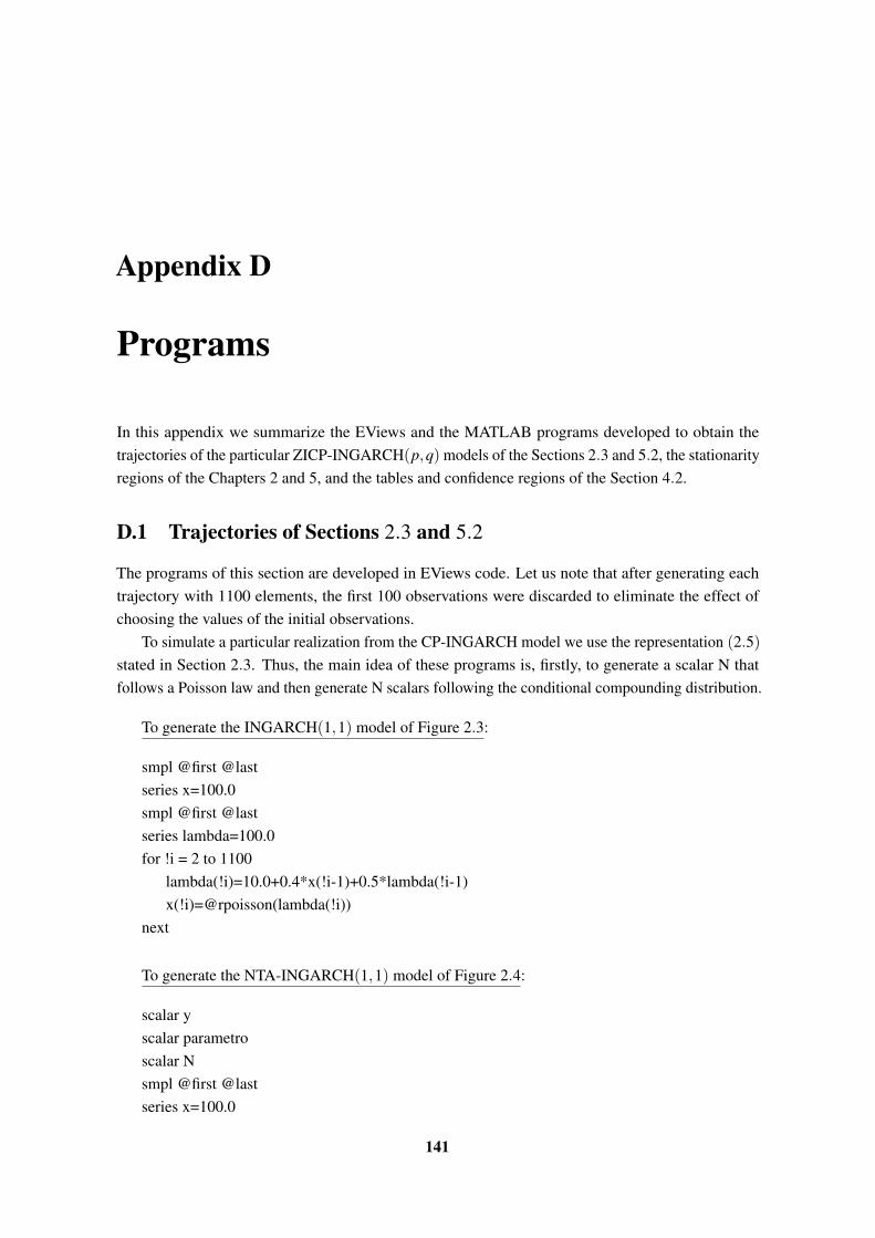
Appendix D
Programs
In this appendix we summarize the EViews and the MATLAB programs developed to obtain thetrajectories of the particular ZICP-INGARCH(p,q) models of the Sections 2.3 and 5.2, the stationarityregions of the Chapters 2 and 5, and the tables and confidence regions of the Section 4.2.
D.1 Trajectories of Sections 2.3 and 5.2
The programs of this section are developed in EViews code. Let us note that after generating eachtrajectory with 1100 elements, the first 100 observations were discarded to eliminate the effect ofchoosing the values of the initial observations.
To simulate a particular realization from the CP-INGARCH model we use the representation (2.5)stated in Section 2.3. Thus, the main idea of these programs is, firstly, to generate a scalar N thatfollows a Poisson law and then generate N scalars following the conditional compounding distribution.
To generate the INGARCH(1,1) model of Figure 2.3:
smpl @first @lastseries x=100.0smpl @first @lastseries lambda=100.0for !i = 2 to 1100
lambda(!i)=10.0+0.4*x(!i-1)+0.5*lambda(!i-1)x(!i)=@rpoisson(lambda(!i))
next
To generate the NTA-INGARCH(1,1) model of Figure 2.4:
scalar yscalar parametroscalar Nsmpl @first @lastseries x=100.0
141

142 Programs
smpl @first @lastseries lambda=100.0scalar phi=2for !i = 2 to 1100
lambda(!i)=10.0+0.4*x(!i-1)+0.5*lambda(!i-1)parametro=lambda(!i)/phiN=@rpoisson(parametro)y=0.0for !j = 1 to N
y=y+@rpoisson(phi)nextx(!i)=y
next
To generate the GEOMP-INGARCH(1,1) model of Figure 2.5:
scalar yscalar contascalar fcumscalar vscalar uscalar pscalar Nsmpl @first @lastseries x=100.0smpl @first @lastseries lambda=100.0scalar r=2for !i = 2 to 1100
lambda(!i)=10.0+0.4*x(!i-1)+0.5*lambda(!i-1)p=r/(r+lambda(!i))N=@rpoisson(r)y=0.0for !j=1 to N
u=@runif(0,1)conta=0v=pfcum=vwhile u >= fcumv=v*(1-p)fcum=fcum+vconta=conta+1

D.1 Trajectories of Sections 2.3 and 5.2 143
wendy=y+conta
nextx(!i)=y
next
To generate the CP-INGARCH(1,1) model of Figure 2.6:
scalar qscalar sseries yseries lambdaseries pseries nscalar xy=0.0lambda=10.0scalar r=5000for !t=2 to 1100
lambda(!t)=10.0+0.4*y(!t-1)+0.5*lambda(!t-1)q=1/((!t)∧2+1)p(!t)=lambda(!t)/(r*q)n(!t)=@rpoisson(p(!t))s=0for !j=1 to n(!t)
x=@rbinom(r,q)s=s+x
nexty(!t)=s
next
To generate the GEOMP2-INARCH(1) model of Figure 2.7:
scalar parametroscalar uscalar fcumscalar contascalar yscalar Nsmpl @first @lastseries x=100.0smpl @first @last

144 Programs
series lambda=100.0scalar p=0.3for !i = 2 to 1100
lambda(!i)=10.0+0.4*x(!i-1)parametro=(p*lambda(!i))/(1-p)N=@rpoisson(parametro)y=0.0for !j = 1 to N
u=@runif(0,1)fcum=pconta=0while u>= fcumconta=conta +1fcum=fcum +p*(1-p)∧(conta)wendy=y+conta
nextx(!i)=y
next
To generate the GP-INARCH(1) model of Figure 2.8:
scalar parametroscalar yscalar uscalar fcumscalar contascalar Nsmpl @first @lastseries x=100.0smpl @first @lastseries lambda=100.0scalar kappa=0.5for !i = 2 to 1100
lambda(!i)=10.0+0.4*x(!i-1)parametro=(1-kappa)*lambda(!i)N=@rpoisson(parametro)y=0.0for !j=1 to N
u=@runif(0,1)fcum=@exp(-kappa)conta=1

D.1 Trajectories of Sections 2.3 and 5.2 145
while u>= fcumconta=conta +1fcum=fcum +((conta*kappa)∧(conta-1)*@exp(-kappa*conta))/@fact(conta)wendy=y+conta
nextx(!i)=y
next
To simulate a particular realization from the ZICP-INGARCH model we use the representation(5.4) stated in Section 5.2. The main idea of the next programs is, firstly, to generate a scalar M thatfollows a Bernoulli law with parameter 1−ω and then, if M= 0, we generate M scalars following theconditional compound Poisson law which have the additional proportion of zeros.
To generate the ZIP-INGARCH(1,1) model of Figure 5.2:
scalar Mscalar Nsmpl @first @lastseries x=44.0smpl @first @lastseries lambda=44.0scalar omega=0.2for !i = 2 to 1100
lambda(!i)=10.0+0.4*x(!i-1)+0.5*lambda(!i-1)M=@rbinom(1,1-omega)if M=0 thenx(!i)=0elsex(!i)=@rpoisson(lambda(!i))endif
next
To generate the ZINTA-INGARCH(1,1) model of Figure 5.3:
scalar Mscalar Nscalar parametroseries x=12.0series lambda=12.0scalar phi=2scalar omega=0.6for !i = 2 to 1100

146 Programs
lambda(!i)=10.0+0.4*x(!i-1)+0.5*lambda(!i-1)M=@rbinom(1,1-omega)if M=0 thenx(!i)=0elseparametro=lambda(!i)/phiN=@rpoisson(parametro)scalar y=0.0for !j = 1 to N
y=y+@rpoisson(phi)nextx(!i)=yendif
next
D.2 Stationarity regions of Sections 3.2 and 5.3
The programs of this section were developed in MATLAB code.To get the weak stationarity regions (αp,βp) ∈ (R+
0 )2 : (1−ω)(1+ v1)α
2p + 2(1−ω)αpβp +
β 2p < 1 of a ZICP-INGARCH(p, p) model with the coefficients α1 = ...=αp−1 = β1 = ...= βp−1 = 0,
under the condition (1−ω)αp +βp < 1 and considering different values for v1, we run the program:
a) function [] = regioes_est_fraca_ZICP_INGARCH_p_p_graf()
grey1 = [0.75,0.75,0.75];grey2 = [0.55,0.55,0.55];grey3 = [0.4,0.4,0.4];alphap = [0.001:0.001:1];betap = [0.001:0.001:1];
B = regiao_est_fraca_zero_iflated_p_p(alphap, betap, 5, 0);C = regiao_est_fraca_zero_iflated_p_p(alphap, betap, 0.5, 0);D = regiao_est_fraca_zero_iflated_p_p(alphap, betap, 0, 0);
t1 = size(B); t2 = size(C); t3 = size(D);i = 1:1:t1(1); j = 1:1:t2(1); k = 1:1:t3(1);f1(i) = B(i,1); g1(i) = B(i,2);f2(j) = C(j,1); g2(j) = C(j,2);f3(k) = D(k,1); g3(k) = D(k,2);
plot(f3(k),g3(k), ’Color’, grey1)hold onplot(f2(j),g2(j), ’Color’, grey2)hold on

D.2 Stationarity regions of Sections 3.2 and 5.3 147
plot(f1(i),g1(i), ’Color’, grey3)xlabel(’alpha_p’)ylabel(’beta_p’)
where
b) function B = regiao_est_fraca_zero_iflated_p_p(alphap, betap, v1, omega)
b1 = size(alphap,2);b2 = size(betap,2);b = b1*b2;A = zeros(b,2);conta = 0;
for i=1:size(alphap,2)for j=1:size(betap,2)
if ((1-omega)*alphap(i) + betap(j))<1aux1 = (1-omega)*(1+v1)*alphap(i)∧2;aux2 = 2*(1-omega)*alphap(i)*betap(j)+betap(j)∧2;if (aux1 + aux2)<1
conta = conta + 1;A(conta,1) = alphap(i);A(conta,2) = betap(j);
endend
endend
B = zeros(conta,2);for i=1:conta
B(i,:)=A(i,:);end
Let us observe that when we run the program regioes_est_fraca_ZICP_INGARCH_p_p_graf weobtain the regions presented in Figure 3.1. To get the regions on the left in Figure 5.6 we consider
B = regiao_est_fraca_zero_iflated_p_p(alphap, betap, 0, 0);C = regiao_est_fraca_zero_iflated_p_p(alphap, betap, 0, 0.4);D = regiao_est_fraca_zero_iflated_p_p(alphap, betap, 0, 0.9);
and for the regions on the right in Figure 5.6 we need to consider
B = regiao_est_fraca_zero_iflated_p_p(alphap, betap, 5, 0);C = regiao_est_fraca_zero_iflated_p_p(alphap, betap, 5, 0.4);D = regiao_est_fraca_zero_iflated_p_p(alphap, betap, 5, 0.9);
instead of the lines 7, 8 and 9 of the program.

148 Programs
To represent the weak stationarity regions of a CP-INGARCH(2,1) process considering differentvalues for the parameter v1 (namely, v1 = 0,0.5,5) and under the condition α1 +α2 +β1 < 1, whichwe presented in figures 3.2 and 3.3 we used the following program:
c) function [] = regiao_est_fraca_CP_INGARCH_2_1()
grey1 = [0.75,0.75,0.75];grey2 = [0.55,0.55,0.55];grey3 = [0.4,0.4,0.4];
B = regiao(0);C = regiao(0.5);D = regiao(5);
t = size(B); t1 = size(C); t2 = size(D);i = 1:1:t(1); j = 1:1:t1(1); k = 1:1:t2(1);f(i) = B(i,1); f1(j) = C(j,1); f2(k) = D(k,1);g(i) = B(i,2); g1(j) = C(j,2); g2(k) = D(k,2);h(i) = B(i,3); h1(j) = C(j,3); h2(k) = D(k,3);
subplot(2,3,1)plot3(f(i),g(i),h(i), ’Color’, grey1)grid onxlabel(’alpha_1’)ylabel(’alpha_2’)zlabel(’beta_1’)
subplot(2,3,2)plot3(f1(j),g1(j),h1(j), ’Color’, grey2)grid onxlabel(’alpha_1’)ylabel(’alpha_2’)zlabel(’beta_1’)
subplot(2,3,3)plot3(f2(k),g2(k),h2(k), ’Color’, grey3)grid onxlabel(’alpha_1’)ylabel(’alpha_2’)zlabel(’beta_1’)
subplot(2,3,4)plot(f(i),g(i), ’Color’, grey1)hold onplot(f1(j),g1(j), ’Color’, grey2)hold on

D.2 Stationarity regions of Sections 3.2 and 5.3 149
plot(f2(k),g2(k), ’Color’, grey3)gridxlabel(’alpha_1’)ylabel(’alpha_2’)title(’View just the X,Y plane’)
subplot(2,3,5)plot(f(i),h(i), ’Color’, grey1)hold onplot(f1(j),h1(j), ’Color’, grey2)hold onplot(f2(k),h2(k), ’Color’, grey3)gridxlabel(’alpha_1’)ylabel(’beta_1’)title(’View just the X,Z plane’)
subplot(2,3,6)plot(g(i),h(i), ’Color’, grey1)hold onplot(g1(j),h1(j), ’Color’, grey2)hold onplot(g2(k),h2(k), ’Color’, grey3)gridxlabel(’alpha_2’)ylabel(’beta_1’)title(’View just the Y,Z plane’)
where we have
d) function B = regiao(v1)
% INPUT:% parameter v1
% OUTPUT:% matrix B containing the points (α1,α2,β1) that belong to the weak% stationarity region for this particular v1
syms alpha1 alpha2 beta1g = obter_zeros(v1);syms f1(alpha1,alpha2,beta1,v1)syms f2(alpha1,alpha2,beta1,v1)syms f3(alpha1,alpha2,beta1,v1)f1(alpha1,alpha2,beta1,v1) = g(1);

150 Programs
f2(alpha1,alpha2,beta1,v1) = g(2);f3(alpha1,alpha2,beta1,v1) = g(3);x = [0.001:0.02:1];y = [0.001:0.02:1];z = [0.001:0.02:1];b1 = size(x,2); b2 = size(y,2); b3 = size(z,2);b = b1*b2*b3;A = zeros(b,3);conta = 0;
for i=1:size(x,2)for j=1:size(y,2)
for k=1:size(z,2)if (x(i) + y(j) + z(k))<1
aux1 = double(f1(x(i),y(j),z(k),v1));aux2 = double(f2(x(i),y(j),z(k),v1));aux3 = double(f3(x(i),y(j),z(k),v1));if (abs(aux1) > 1) && (abs(aux2) > 1) && (abs(aux3) > 1)
conta = conta + 1;A(conta,1) = x(i);A(conta,2) = y(j);A(conta,3) = z(k);
endend
endend
end
B = zeros(conta,3);for i=1:conta
B(i,:)=A(i,:);end
and also
e) function g = obter_zeros(v1)
% INPUT:% parameter v1
% OUTPUT:% the roots of the equation detP(z) = 0 for this particular v1
syms alpha1 alpha2 beta1aux1 = (alpha1+beta1)∧2*alpha2+alpha2∧2;aux2 = v1*(alpha2∧2+alpha1∧2*alpha2+2*alpha1*alpha2*beta1);

D.3 Simulation Study - Section 4.2 151
p1 = alpha2∧3+v1*alpha2∧3;p2 = aux1+aux2;p3 = (alpha1+beta1)∧2+alpha2+v1*alpha1∧2;p = [p1 -p2 -p3 1];g = roots(p);
D.3 Simulation Study - Section 4.2
The following programs are developed to use in MATLAB.In what concerns the Table 4.1 and Table 4.2 we developed the following algorithm:
a) function [g] = valores(alpha0, alpha1, n)
% INPUT:% real parameters (α0, α1) of the INARCH(1) model% length n of the trajectory% OUTPUT:% means, variances and covariances of the estimates
A = zeros(1000,2);b1 = ones(1000,1);b2 = ones(1000,1);u1 = ones(1000,1);u2 = ones(1000,1);d = zeros(1000,1);
for i=1:1000x = valores_trajectoria_Poisson(alpha0, alpha1, n);est = estimativaCLS_Poisson(x);A(i,1) = est(1);A(i,2) = est(2);
end
% A is the matrix that in the column j has the estimates for the parameter α j,% j = 0,1, that we obtain from the 1000 trajectories that were generated
S = sum(A);% S is the 1x2 matrix that in the column j has the sum of the estimates of α j, j = 0,1
media(1) = S(1)/1000;media(2) = S(2)/1000;b1 = media(1)*b1;b2 = media(2)*b2;B = [b1 b2];% B is the 1000x2 matrix that in the column j has the mean of the 1000% estimates of α j, j = 0,1

152 Programs
D = A - B;C = D.∧2;V = sum(C);variancia(1) = n*(V(1)/1000);variancia(2) = n*(V(2)/1000);u1 = alpha0*u1;u2 = alpha1*u2;U = [u1 u2];R = (U - A).∧2;Q = sum(R);standarderror(1) = sqrt(Q(1)/1000);standarderror(2) = sqrt(Q(2)/1000);
for j=1:1000d(j) = D(j,1)*D(j,2);
end
covariancia = n*(sum(d)/1000);g = [media(1) media(2) variancia(1) standarderror(1) variancia(2) standarderror(2)
covariancia];
where we have
b) function [y] = valores_trajectoria_Poisson(alpha0, alpha1, n)
% INPUT:% parameters α0, α1
% length n of the trajectory% OUTPUT:% one trajectory with n elements of an INARCH(1) process with parameters α0 and α1
x = zeros(1,n+100);y = zeros(1,n);lambda = zeros(1,n+100);lambda(1) = alpha0/(1-alpha1);
for i=2:n+100lambda(i)= alpha0 + alpha1*x(i-1);x(i) = poissrnd(lambda(i));
end
for k=1:ny(k)=x(k+100);
end
and to calculate the CLS estimates we use

D.3 Simulation Study - Section 4.2 153
c) function [estimativas] = estimativaCLS_Poisson(y)
% INPUT:% trajectory y% OUTPUT:% CLS estimates of the parameters (α0,α1) of the process INARCH(1) from trajectory y
n=length(y);soma = 0;soma0 = 0;
for i=2:nsoma = soma + y(i)*y(i-1);soma0 = soma0 + y(i-1)*y(i-1);
end
somar=0;mediaemp=sum(y)/n;
for i=1:nsomar= somar + (y(i)- mediaemp)∧2;
end
soma1=sum(y)-y(1);soma2=sum(y)-y(n);soma3=1/(n-1)*soma1*soma2;soma4=1/(n-1)*soma2*soma2;
alpha1=(soma -soma3)/(soma0-soma4);alpha0=(soma1-alpha1*soma2)/(n-1);estimativas(1)=alpha0;estimativas(2)=alpha1;
Concerning the tables 4.3 and 4.5 we used the following algorithm:
d) function [g] = valores_tabelas(alpha0, alpha1, b, n)
% INPUT:% real parameters (α0, α1, φ ) of the NTA-INARCH(1) model% (b corresponds to parameter φ )% OUTPUT:% means, variances and covariances of the estimates
A = zeros(1000,3);b1 = ones(1000,1);b2 = ones(1000,1);b3 = ones(1000,1);

154 Programs
d = zeros(1000,1);e = zeros(1000,1);f = zeros(1000,1);
for i=1:1000x = valores_trajectoria_NTA(alpha0, alpha1, b, n);est = estimativaCLS_NTA(x);A(i,1) = est(1);A(i,2) = est(2);A(i,3) = est(3);
end
S = sum(A);media(1) = S(1)/1000;media(2) = S(2)/1000;media(3) = S(3)/1000;b1 = media(1)*b1;b2 = media(2)*b2;b3 = media(3)*b3;B = [b1 b2 b3];D = A - B;C = D.∧2;V = sum(C);variancia(1) = n*(V(1)/1000);variancia(2) = n*(V(2)/1000);variancia(3) = V(3)/1000;varb = n*variancia(3);
for j=1:1000d(j) = D(j,1)*D(j,2);e(j) = D(j,1)*D(j,3);f(j) = D(j,2)*D(j,3);
end
covariancia(1) = n*(sum(d)/1000);covariancia(2) = sum(e)/1000;covariancia(3) = sum(f)/1000;
corr(1) = covariancia(1)/(sqrt(variancia(1))*sqrt(variancia(2)));corr(2) = covariancia(2)/(sqrt(variancia(1)/n)*sqrt(variancia(3)));corr(3) = covariancia(3)/(sqrt(variancia(2)/n)*sqrt(variancia(3)));
g = [media(1) media(2) media(3) variancia(1) variancia(2) varb covariancia(1) corr(1)corr(2) corr(3)];
where to generate the trajectory of the NTA-INARCH(1) process we use the program:

D.3 Simulation Study - Section 4.2 155
e) function [y] = valores_trajectoria_NTA(alpha0, alpha1, phi, n)
% INPUT:% parameters α0, α1 and φ
% length n of the trajectory% OUTPUT:% trajectory with n elements of an NTA-INARCH(1) process with parameters α0, α1, φ
x = zeros(1,n+100);y = zeros(1,n);lambda = zeros(1,n+100);lambda(1) = alpha0/(1-alpha1);
for i=2:n+100lambda(i)= alpha0 + alpha1*x(i-1);parametro=lambda(i)/phi;N=poissrnd(parametro);z=0;for j=1:N
z=z+poissrnd(phi);endx(i)=z;
end
for k=1:ny(k)=x(k+100);
end
and to calculate the estimates of the three parameters we use
f) function [estimativas] = estimativaCLS_NTA(y)
% INPUT:% trajectory y% OUTPUT:% CLS estimates of the parameters (α0,α1) and estimate the parameter φ based on% the moments estimation method of the process NTA-INARCH(1) from trajectory y
n=length(y);soma = 0;soma0 = 0;
for i=2:nsoma = soma + y(i)*y(i-1);soma0 = soma0 + y(i-1)*y(i-1);
end

156 Programs
somar=0;mediaemp=sum(y)/n;for i=1:n
somar= somar + (y(i)- mediaemp)∧2;end
VarEmp=somar/n;soma1=sum(y)-y(1);soma2=sum(y)-y(n);soma3=1/(n-1)*soma1*soma2;soma4=1/(n-1)*soma2*soma2;
alpha1=(soma -soma3)/(soma0-soma4);alpha0=(soma1-alpha1*soma2)/(n-1);phi= -1 + ((1-alpha1)*(1-alpha1∧2)*VarEmp)/alpha0;estimativas(1)=alpha0;estimativas(2)=alpha1;estimativas(3)=phi;
The program to get the values presented in Table 4.4 is quite similar to the above. In fact, in theprogram valores_tabelas(alpha0, alpha1, b, n) we only need to change
"x = valores_trajectoria_NTA(alpha0, alpha1, b, n);" to"x = valores_trajectoria_GEOMP2(alpha0, alpha1, b, n);"
and"est = estimativaCLS_NTA(x);" to"est = estimativaCLS_GEOMP2(x);"
where now b corresponds to the parameter p∗, and then consider
g) function [y] = valores_trajectoria_GEOMP2(alpha0, alpha1, p, n)
% INPUT:% parameters α0, α1 and p% length n of the trajectory% OUTPUT:% trajectory with n elements of a GEOMP2-INARCH(1) process% with parameters α0, α1, px = zeros(1,n+100);y = zeros(1,n);lambda = zeros(1,n+100);lambda(1) = alpha0/(1-alpha1);
for i=2:n+100lambda(i)= alpha0 + alpha1*x(i-1);parametro=(p*lambda(i))/(1-p);

D.3 Simulation Study - Section 4.2 157
N=poissrnd(parametro);z=0;for j=1:N
z=z+ geornd(p);endx(i)=z;
end
for k=1:ny(k)=x(k+100);
end
and
h) function [estimativas] = estimativaCLS_GEOMP2(y)
% INPUT:% trajectory y% OUTPUT:% CLS estimates of the parameters (α0,α1) and estimate the parameter p based on the% moments estimation method of the process GEOMP2-INARCH(1) from trajectory y
n=length(y);soma=0;soma0=0;
for i=2:nsoma = soma + y(i)*y(i-1);soma0 = soma0 + y(i-1)*y(i-1);
end
somar=0;mediaemp=sum(y)/n;
for i=1:nsomar=somar + (y(i)- mediaemp)∧2;
end
VarEmp=somar/n;soma1=sum(y)-y(1);soma2=sum(y)-y(n);soma3=1/(n-1)*soma1*soma2;soma4=1/(n-1)*soma2*soma2;
alpha1=(soma -soma3)/(soma0-soma4);alpha0=(soma1-alpha1*soma2)/(n-1);outro= (1-alpha1)/alpha0;
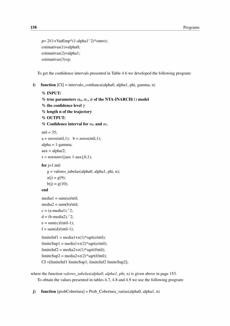
158 Programs
p= 2/(1+VarEmp*(1-alpha1∧2)*outro);estimativas(1)=alpha0;estimativas(2)=alpha1;estimativas(3)=p;
To get the confidence intervals presented in Table 4.6 we developed the following program:
i) function [CI] = intervalo_confianca(alpha0, alpha1, phi, gamma, n)
% INPUT:% true parameters α0, α1, φ of the NTA-INARCH(1) model% the confidence level γ
% length n of the trajectory% OUTPUT:% Confidence interval for m0 and m1
ntil = 35;a = zeros(ntil,1); b = zeros(ntil,1);alpha = 1-gamma;aux = alpha/2;z = norminv([aux 1-aux],0,1);
for j=1:ntilg = valores_tabelas(alpha0, alpha1, phi, n);a(j) = g(9);b(j) = g(10);
end
media1 = sum(a)/ntil;media2 = sum(b)/ntil;c = (a-media1).∧2;d = (b-media2).∧2;e = sum(c)/(ntil-1);f = sum(d)/(ntil-1);
limiteInf1 = media1+z(1)*sqrt(e/ntil);limiteSup1 = media1+z(2)*sqrt(e/ntil);limiteInf2 = media2+z(1)*sqrt(f/ntil);limiteSup2 = media2+z(2)*sqrt(f/ntil);CI =[limiteInf1 limiteSup1; limiteInf2 limiteSup2];
where the function valores_tabelas(alpha0, alpha1, phi, n) is given above in page 153.To obtain the values presented in tables 4.7, 4.8 and 4.9 we use the following program:
j) function [probCobertura] = Prob_Cobertura_varias(alpha0, alpha1, n)

D.3 Simulation Study - Section 4.2 159
% INPUT:% true parameters α0, α1 of the INARCH(1) model% length n of the trajectory% OUTPUT:% Estimated coverage probabilities of the confidence region for three different% confidence levels: 0.9, 0.95 and 0.99
v0=1; d0=1;B = matriz(alpha0, alpha1, v0, d0);% gamma is the confidence levelgamma = [0.9, 0.95, 0.99];conta1 = 0; conta2 = 0; conta3 = 0;% determine the gamma-quantile of the chi-squared distributionz1 = chi2inv(gamma(1),2)/(n-1);z2 = chi2inv(gamma(2),2)/(n-1);z3 = chi2inv(gamma(3),2)/(n-1);
for i=1:10000x = valores_trajectoria_Poisson(alpha0, alpha1, n);est = estimativaCLS_Poisson(x);y = [est(1)-alpha0; est(2)-alpha1];CR = y’*B*y;if (CR < z1)
conta1 = conta1 + 1;endif (CR < z2)
conta2 = conta2 + 1;endif (CR < z3)
conta3 = conta3 + 1;end
end
probCobertura(1) = conta1/10000;probCobertura(2) = conta2/10000;probCobertura(3) = conta3/10000;
where
k) function [B] = matriz(alpha0, alpha1, v0, d0)
% OUTPUT:% asymptotic matrix V−1WV−1
A = zeros(2,2);

160 Programs
num1 = v0∧2+(d0-v0∧2)*alpha1*(1+alpha1-alpha1∧2)+(3*v0∧2-d0)*alpha1∧4;num2 = alpha1*(d0+(3*v0∧2-d0)*alpha1∧2);num3 = (1+alpha1)*num2;den1 = v0*(1+alpha1+alpha1∧2);den2 = den1*alpha0;A(1,1) = (alpha0/(1-alpha1))*(alpha0*(1+alpha1)+num1/den1);A(2,2) = (1-alpha1∧2)*(1+num2/den2);A(1,2) = v0*alpha1-alpha0*(1+alpha1)-num3/den1;A(2,1) = A(1,2);B = inv(A);
Let us note that when we consider the parameters α0 = 2, α1 = 0.2 and n = 100, we obtain thefirst element of tables 4.7, 4.8 and 4.9. Then we need to run again the program to get the other values.