composite load model evaluation - discovery in action · composite load model evaluation ... this...

PNNL-16916

Composite Load Model Evaluation N. Lu A. Qiao September 2007 Prepared for the Bonneville Power Administration Under contract, 00162-00033 With the U.S. Department of Energy Under DE-AC05-76RL01830

DISCLAIMER

This report was prepared as an account of work sponsored by an agency of the United States Government. Neither the United States Government nor any agency thereof, nor Battelle Memorial Institute, nor any of their employees, makes any warranty, express or implied, or assumes any legal liability or responsibility for the accuracy, completeness, or usefulness of any information, apparatus, product, or process disclosed, or represents that its use would not infringe privately owned rights. Reference herein to any specific commercial product, process, or service by trade name, trademark, manufacturer, or otherwise does not necessarily constitute or imply its endorsement, recommendation, or favoring by the United States Government or any agency thereof, or Battelle Memorial Institute. The views and opinions of authors expressed herein do not necessarily state or reflect those of the United States Government or any agency thereof.

PACIFIC NORTHWEST NATIONAL LABORATORY

operated by BATTELLE

for the UNITED STATES DEPARTMENT OF ENERGY

under Contract DE-AC0576RL01830

Printed in the United States of America

Available to DOE and DOE contractors from the Office of Scientific and Technical Information,

P.O. Box 62, Oak Ridge, TN 37831-0062; ph: (865) 576-8401 fax: (865) 576-5728

email: [email protected]

Available to the public from the National Technical Information Service, U.S. Department of Commerce, 5285 Port Royal Rd., Springfield, VA 22161

ph: (800) 553-6847 fax: (703) 605-6900

email: [email protected] online ordering: http://www.ntis.gov/ordering.htm

This document was printed on recycled paper. (8/00)

http://www.ntis.gov/ordering.htm�

Composite Load Model Evaluation N. Lu A. Qiao September 2007 Prepared for the Bonneville Power Administration Under contract, 00162-00033 With the U.S. Department of Energy Under DE-AC05-76RL01830

Pacific Northwest National Laboratory Richland, Washington 99352

iii

SUMMARY This final report is prepared for Bonneville Power Administration to document the methodology and

procedure used to evaluate the new composite load model, CMPLDW, which is developed by GE Energy. The composite load model structure is provided by the WECC load modeling task force. It is to be used to represent behaviors of different end-user components. GE Energy has implemented this composite load model with a new function CMPLDW in its power system simulation software package, Positive Sequence Load Flow (PSLF). Pacific Northwest National Laboratory (PNNL) and BPA joined forces and conducted the evaluation of the CMPLDW and tested its parameter settings. The PNNL testing results are documented in this report.

iv

Table of Contents

Summary.....................................................................................................................................................iii

1. Introduciton......................................................................................................................................... 1

2. Model Evaluation Methodology ........................................................................................................ 3

3. Evaluation Test Procedures and results............................................................................................ 5

3.1 Test 1: Compare Motor-W with CMPLDW ..................................................................................5 3.2 Test 2: Static Load Only Simulations............................................................................................ 6 3.3 Test 3: Four Motor Loads............................................................................................................. 7

4. Conclusion ........................................................................................................................................... 8 Appendix I - Comparison with MOTOR W ................................................................................................. 9 Appendix II - Static Load Simulation ......................................................................................................... 13 Appendix III - Four Motor Dynamic Simulations ...................................................................................... 16 Appendix IV - One motor plus one static load ........................................................................................... 25 Appendix V - WECC Composite Load Model (CMPLDW) Specifications ..............................................27

v

Figures

Figure 1: The Composite Load Model Structure ......................................................................................... 1

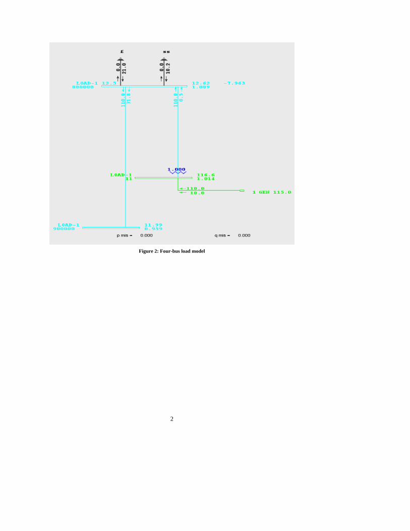
Figure 2: Four-bus load model...................................................................................................................... 2

Figure 3: Sample testing signals (oscillation, voltage hump, voltage rampup and rampdown, and voltage sags) ...................................................................................................................................................... 4

Figure 4: An example *.dyd file ................................................................................................................... 5

Tables

Table 1: Compare with Motor W.................................................................................................................. 6

Table 2: Static load simulation...................................................................................................................... 7

Table 3: Four Motor Loads ........................................................................................................................... 7

1

1. INTRODUCITON

The WECC load modeling task force has dedicated its effort in the past few years to developing a composite load model that can represent behaviors of different end-user components. The modeling structure of the composite load model recommended by the WECC load modeling task force has been illustrated in Figure 1. GE Energy has implemented this composite load model with a new function CMPLDW in its power system simulation software package, Positive Sequence Load Flow (PSLF).

For the last several years, Bonneville Power Administration (BPA) has taken the lead and collaborated with GE Energy to develop the new composite load model. Pacific Northwest National Laboratory (PNNL) and BPA joined forces and conducted the evaluation of the CMPLDW and tested its parameter settings to make sure that:

• the model initialized properly

• all the parameter settings were functioning

• the simulation results were as expected.

The PNNL effort focused on testing the CMPLDW in a four-bus system, as shown in Figure 2. Exhaustive testing on each parameter setting has been performed to guarantee each setting works. This report is a summary of the PNNL testing results and conclusions.

Figure 1: The Composite Load Model Structure

2

Figure 2: Four-bus load model

3

2. MODEL EVALUATION METHODOLOGY

The most rigorous way to build confidence in models is to compare model simulation results with field measurements. However, because the CMPLDW model is built upon several known load models, PNNL’s evaluation is, therefore, conducted by comparing the simulation results obtained by the validated model and the CMPLDW model.

1. Motor load modeling: Set the static load to zero and operate only one motor load. For example, Motor A is running and Motor B, C, and D are offline. Then, compare the simulation results obtained by CMPLDW with the results by Motor W.

2. Static load modeling: compare with the direct calculations.

3. Test each parameter setting: Exhaustive tests are run, in which only one parameter is changed at a time to observe the results.

Please refer to Appendix V of the GE Energy: WECC Composite Load Model (CMPLDW) Specifications for the parameter settings.

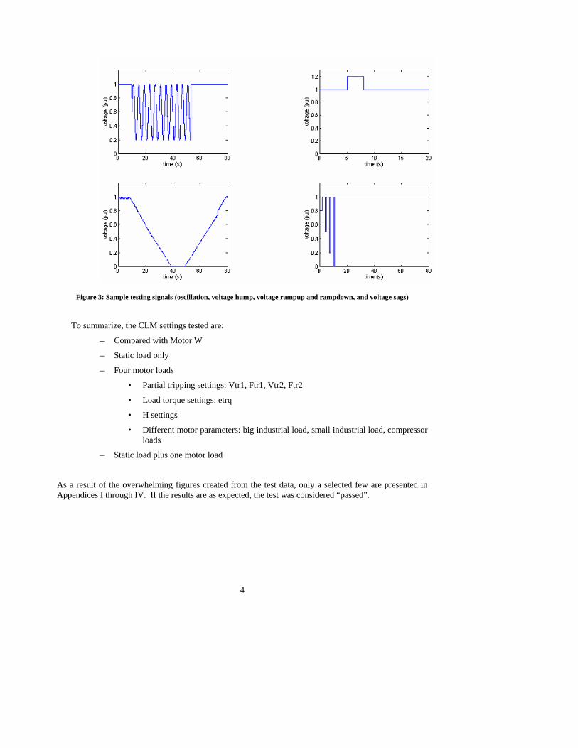
CSV files are used to create the testing signals. PSLF playback function is used to inject different testing signals as shown in Figure 3, which include:

– Voltage sags

– Voltage ramp

– Voltage oscillation

– Voltage hump

– Frequency sag

– Frequency oscillation

– Frequency ramp

4

Figure 3: Sample testing signals (oscillation, voltage hump, voltage rampup and rampdown, and voltage sags)

To summarize, the CLM settings tested are:

– Compared with Motor W

– Static load only

– Four motor loads

• Partial tripping settings: Vtr1, Ftr1, Vtr2, Ftr2

• Load torque settings: etrq

• H settings

• Different motor parameters: big industrial load, small industrial load, compressor loads

– Static load plus one motor load

As a result of the overwhelming figures created from the test data, only a selected few are presented in Appendices I through IV. If the results are as expected, the test was considered “passed”.

5

3. EVALUATION TEST PROCEDURES AND RESULTS

3.1 Test 1: Compare Motor W with CMPLDW

In this test, all the motor parameters were set equal. The fraction of the motor load fraction to be "Fma" 1.0 "Fmb" 0.0 "Fmc" 0.0 "Fmd" 0.0 "Fdl" 0.0 /, or "Fma" 0.0 "Fmb" 1.0 "Fmc" 0.0 "Fmd" 0.0 "Fdl" 0.0 /, or "Fma" 0.0 "Fmb" 0.0 "Fmc" 1.0 "Fmd" 0.0 "Fdl" 0.0 /, or "Fma" 0.0 "Fmb" 0.0 "Fmc" 0.0 "Fmd" 1.0 "Fdl" 0.0 /. An example of the *.dyd files is shown in Figure 4.

Figure 4: An example *.dyd file

The following scenarios were tested and results are included in Appendix I and also summarized in Table 1.

lodrep

cmpldw 11 "LOAD-1 " 115.00 "A " : #3 mva=100.410004 "Bss" 0.3057 "Rfdr" 0.03465 "Xfdr" 0.04331 "Fb" 0.00/

"Xxf" 0.08 "TfixHS" 1 "TfixLS" 1 "LTC" 1 "Tmin" 1 "Tmax" 1 "step" 0.00625 /

"Vmin" 1.025 "Vmax" 1.04 "Tdel" 30 "Ttap" 5 "Rcomp" 0 "Xcomp" 0 /

"Fma" 1.0 "Fmb" 0.0 "Fmc" 0.0 "Fmd" 0.0 "Fdl" 0.0 /

"Pfs" 0.99806 "P1e" 2 "P1c" 0 "P2e" 1 "P2c" 0 "Pfreq" 1 /

"Q1e" 2 "Q1c" 0 "Q2e" 1 "Q2c" 0 "Qfreq" -1 /

"MtpA" 3 "LfmA" 0.85 "RsA" 0.02 "LsA" 3.58 "LpA" 0.177 "LppA" 0.177 "TpoA" 0.56 "TppoA" 0.02 /

"HA" 0.3 "atrqA" 0 "btrqA" 0 "dtrqA" 1 "etrqA" 2 /

"Vtr1A" 0 "Ttr1A" 99999 "Ftr1A" 0 "Vrc1A" 0.8 "Trc1A" 0.5 /

"Vtr2A" 0.4 "Ttr2A" 0.02 "Ftr2A" 0 "Vrc2A" 999 "Trc2A" 999

6

Table 1: Compare with Motor W

Scenarios Pass Not pass

Voltage Sags

Voltage Ramp

Voltage Oscillation

Voltage Hump

Frequency Sag

Frequency Oscillation

Frequency Ramp

3.2 Test 2: Static Load Only Simulations

P and Q of the static load model can be described in the following equations:

)*1)(3)()(1( 2

02

1

00 fpfP

VVP

VVcPPP eP

CeP Δ+++=

)*1)(3)()(1( 2

02

1

00 fpfQ

VVQ

VVcQQQ eQ

CeQ Δ+++=

In the static load simulation, the motor fraction was set to zero,

"Fma" 0 "Fmb" 0 "Fmc" 0 "Fmd" 0 "Fdl" 1 / "Pfs" 0.96187

and three cases were analyzed. The simulation parameters and results are included in Appendix II and

also summarized in Table 2.

.

7

Table 2: Static load simulation


CASE 1: "P1e" 2 "P1c" 0 "P2e" 1 "P2c" 1 "Pfreq" 0 /

"Q1e" 2 "Q1c" 0 "Q2e" 1 "Q2c" 1 "Qfreq" 0 /

CASE2: "P1e" 2 "P1c" 1 "P2e" 1 "P2c" 0 "Pfreq" 0 /

"Q1e" 2 "Q1c" 1 "Q2e" 1 "Q2c" 0 "Qfreq" 0

CASE3 "P1e" 2 "P1c" 0 "P2e" 1 "P2c" 0 "Pfreq" 0 /

"Q1e" 2 "Q1c" 0 "Q2e" 1 "Q2c" 0 "Qfreq" 0 /

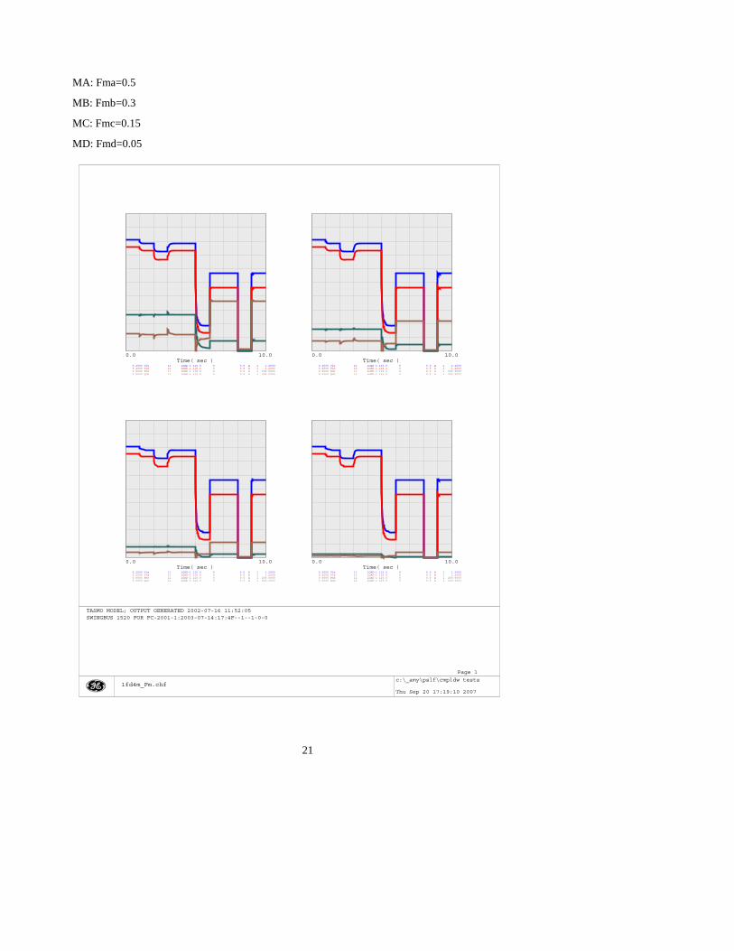
3.3 Test 3: Four Motor Loads

In the four motor dynamic simulations, the motor parameters of MA, Mb, MC and MD were varied one at a time, while the rest of the parameters remained the same. The simulation parameters and results are attached in Appendix III and also summarized in Table 3.

Table 3: Four Motor Loads


Vary H, set etrq=0

Vary H, set etrq=2

Vary etrq

Vary Rs

Vary Fm

Vary Vtr2

Vary Ftr2

Vary Vtr1, set Ttr1=2

8

4. CONCLUSION

After extensive testing, the authors conclude that the CMPLDW model is correctly implemented and all the parameter settings are functioning properly.

9

Appendix I - Comparison with MOTOR W

13

Appendix II - Static Load Simulation

14

Voltage rampdown and rampup

Voltage sags

15

0.2000 Vls 11 LOAD-1 115.0 0 0.0 A 1 1.2000 0.2000 Vld 11 LOAD-1 115.0 0 0.0 A 1 1.2000 0.0000 Pst 11 LOAD-1 115.0 0 0.0 A 1 200.0000 0.0000 Qst 11 LOAD-1 115.0 0 0.0 A 1 200.0000

Time( sec )0.0 10.0

TASMO MODEL; OUTPUT GENERATED 2002-07-16 11:52:05SWINGBUS 1520 FOR FC-2001-1:2003-07-14:17:4F--1--1-0-0

c:\_amy\pslf\cmpldw tests

Thu Sep 20 15:37:52 2007

Page 1

1fd4m_sta1.chf


Time( sec )0.0 10.0



Thu Sep 20 15:39:08 2007

Page 1

1fd4m_sta2.chf

CASE 1: "P1e" 2 "P1c" 0 "P2e" 1 "P2c" 1 "Pfreq" 0 / "Q1e" 2 "Q1c" 0 "Q2e" 1 "Q2c" 1 "Qfreq" 0 /

CASE2: "P1e" 2 "P1c" 1 "P2e" 1 "P2c" 0 "Pfreq" 0 / "Q1e" 2 "Q1c" 1 "Q2e" 1 "Q2c" 0 "Qfreq" 0


Time( sec )0.0 10.0



Thu Sep 20 15:36:24 2007

Page 1

1fd4m_sta3.chf

CASE3 "P1e" 2 "P1c" 0 "P2e" 1 "P2c" 0 "Pfreq" 0 / "Q1e" 2 "Q1c" 0 "Q2e" 1 "Q2c" 0 "Qfreq" 0 /

16

Appendix III - Four Motor Dynamic Simulations

17

MA: HA=0.6, etrqA=0

MB: HB=0.4, etrqB=0

MC: HC=0.2, etrqC=0

MD: HD=0.05, etrqD=0

0.2000 Vls 11 LOAD-1 115.0 0 0.0 A 1 1.2000 0.2000 Vld 11 LOAD-1 115.0 0 0.0 A 1 1.2000 0.0000 Pma 11 LOAD-1 115.0 0 0.0 A 1 200.0000 0.0000 Qma 11 LOAD-1 115.0 0 0.0 A 1 200.0000

Time( sec )0.0 10.0

0.2000 Vls 11 LOAD-1 115.0 0 0.0 A 1 1.2000 0.2000 Vld 11 LOAD-1 115.0 0 0.0 A 1 1.2000 0.0000 Pmb 11 LOAD-1 115.0 0 0.0 A 1 200.0000 0.0000 Qmb 11 LOAD-1 115.0 0 0.0 A 1 200.0000

Time( sec )0.0 10.0

0.2000 Vls 11 LOAD-1 115.0 0 0.0 A 1 1.2000 0.2000 Vld 11 LOAD-1 115.0 0 0.0 A 1 1.2000 0.0000 Pmc 11 LOAD-1 115.0 0 0.0 A 1 200.0000 0.0000 Qmc 11 LOAD-1 115.0 0 0.0 A 1 200.0000

Time( sec )0.0 10.0

0.2000 Vls 11 LOAD-1 115.0 0 0.0 A 1 1.2000 0.2000 Vld 11 LOAD-1 115.0 0 0.0 A 1 1.2000 0.0000 Pmd 11 LOAD-1 115.0 0 0.0 A 1 200.0000 0.0000 Qmd 11 LOAD-1 115.0 0 0.0 A 1 200.0000

Time( sec )0.0 10.0



Thu Sep 20 16:32:25 2007

Page 1

1fd4m_H.chf

18

MA: HA=0.6, etrqA=2

MB: HB=0.4, etrqB=2

MC: HC=0.2, etrqC=2

MD: HD=0.05, etrqD=2


Time( sec )0.0 10.0


Time( sec )0.0 10.0


Time( sec )0.0 10.0


Time( sec )0.0 10.0



Thu Sep 20 16:28:26 2007

Page 1

1fd4m_H.chf

19

MA: HA=0.3, etrqA=2

MB: HB=0.3, etrqB=1

MC: HC=0.3, etrqC=0.5

MD: HD=0.3, etrqD=0


Time( sec )0.0 10.0


Time( sec )0.0 10.0


Time( sec )0.0 10.0


Time( sec )0.0 10.0



Thu Sep 20 16:53:47 2007

Page 1

1fd4m_etrq.chf

20

MA: RsA=0.0113

MB: RsB=0.015

MC: RsC=0.025

MD: RsD=0.053


Time( sec )0.0 10.0


Time( sec )0.0 10.0


Time( sec )0.0 10.0


Time( sec )0.0 10.0



Thu Sep 20 16:42:09 2007

Page 1

1fd4m_Rs.chf

21

MA: Fma=0.5

MB: Fmb=0.3

MC: Fmc=0.15

MD: Fmd=0.05


Time( sec )0.0 10.0


Time( sec )0.0 10.0


Time( sec )0.0 10.0


Time( sec )0.0 10.0



Thu Sep 20 17:19:10 2007

Page 1

1fd4m_Fm.chf

22

MA: Vtr2A=0.9

MB: Vtr2B=0.6

MC: Vtr2C=0.3

MD: Vtr2D=0.1


Time( sec )0.0 10.0


Time( sec )0.0 10.0


Time( sec )0.0 10.0


Time( sec )0.0 10.0



Thu Sep 20 16:59:02 2007

Page 1

1fd4m_Vtr.chf

23

MA: Ftr2A=0.9

MB: Ftr2B=0.6

MC: Ftr2C=0.3

MD: Ftr2D=0.1


Time( sec )0.0 10.0


Time( sec )0.0 10.0


Time( sec )0.0 10.0


Time( sec )0.0 10.0



Thu Sep 20 17:05:26 2007

Page 1

1fd4m_Ftr.chf

24

MA: Vtr1A= 0.9, Ttr1A= 2

MB: Vtr1B= 0.6, Ttr1B= 2

MC: Vtr1C= 0.3, Ttr1C= 2

MD: Vtr1D= 0.1, Ttr1D= 2


Time( sec )0.0 10.0


Time( sec )0.0 10.0


Time( sec )0.0 10.0


Time( sec )0.0 10.0



Thu Sep 20 17:52:58 2007

Page 1

1fd4m_Vtr1.chf

25

Appendix IV - One motor plus one static load

26

Voltage Sags

27

Appendix V - WECC Composite Load Model (CMPLDW) Specifications

28

WECC Composite Load Model (CMPLDW) Specifications

By Bill Price, GE Energy June 8, 2007

• Changes from previous (Feb. 8) specification version are in red. • Features that are not yet implemented in PSLF V16.1 are in green. • Overall Specifications

• The overall structure of the CMPLDW model is shown in Figure 1.

• Any load can be represented in dynamic simulations by a CMPLDW model. All of the P and Q of the load will be included in the CMPLDW model.

Figure 1 CMPLDW Model Structure

M

Static

Substation

Load Bus

System bus (230, 115, 69-kV) M

M

Motor A Feeder LTC

Bss Bf1

Motor B

Motor C

M Motor D

Low-side bus

Bf2

Discharge Lighting

R, X

29

• Fractions of the load can be tripped by relay action via the load shed signal. Such tripping will simulate tripping an equivalent amount of aggregate feeder and of each load element, but not the substation transformer or capacitor (Bss).

• Static Load Model equations:

P = Po * (P1c * V/Vo P1e + P2c * V/Vo P2e + P3 ) * (1 + Pf * Δf )

Q = Qo * (Q1c * V /Vo Q1e + Q2c * V /Vo Q2e + Q3 ) * (1 + Qf * Δf )

Po = Pload ( 1. – Fma – Fmb – Fmc - Fmd)

Qo = Po * tan ( acos(PFs) ) = Po * sqrt(PFs-2 – 1.)

P3 = 1. – P1c – P2c

Q3 = 1. – Q1c – Q2c

Convert to constant G, B below specified V (solpar.vlbrk)

• Motor Mechanical Load Model:

Tm = Tmo * (a * ω2 + b * ω + c + d * ωe)

c = 1. – a – b – d

[WWP - Suggest replacing with Pm = Pmo * ωe for consistency with

motorw and fewer input parameters.]

• Shunt capacitance – The feeder capacitors (Bf1 and Bf2) will be computed during initialization of the dynamic simulation to produce the total Q at the system bus. Calculation of Bf1 uses input parameter fb (fraction of B at substation) based on assumed motor power factor of 0.8. After motor initialization, Bf2 is set to remaining required B.

• If LTC data is present for substation transformer, initial tap is set to put low side voltage approximately in middle of Vmin to Vmax range.

• For each composite load model, input data will be:

• Location – bus number, (name, kV), load ID • MVA=xxx – feeder & xfmr MVA base

- if xxx > 0., xxx is the MVA base. - if xxx < 0, abs. value = loading factor = load MW / MVA base - if xxx = 0., loading factor = default value (0.8)

• Bss - Substation shunt B (pu of MVA base) • Feeder

- Rfdr - Feeder R (pu of MVA base)

30

- Xfdr - Feeder X (pu of MVA base) - Fb –fraction of feeder reactive compensation applied at the substation

end of the feeder If Xfdr = 0., feeder is omitted, but feeder capacitor is included.

• Substation transformer If ( xxf > jumper threshold), include the following: - Xxf – transformer reactiance – p.u. of xfmr MVA base - Tfixhs – High-side fixed xfmr tap - Tfixls – Low-side fixed xfmr tap - LTC – LTC flag – (1=active; 0=inactive) - Tmin - LTC min tap (on low side) - Tmax - LTC max tap (on low side) - Step - LTC Tstep (on low side) - Vmin - LTC Vmin (low side pu) - Vmax - LTC Vmax (low side pu) - Tdel - LTC Control time delay (sec.) - Ttap - LTC Tap adjustment time delay (sec.) - Rcmp - LTC Rcomp (pu of xfmr MVA base) - Xcmp - LTC Xcomp (pu of xfmr MVA base)

• Load composition - Fma - Motor A fraction - Fmb - Motor B fraction - Fmc - Motor C fraction - Fmd - Motor D fraction - Fdl – Discharge Lighting fraction - NOTE: If sum < 1., remainder is static load; if sum > 1, fractions are

nomalized to 1. and there will be no static load. • Static load parameters

- PFs - Power factor - P1e - P1 exponent - P1c - P1 coefficient - P2e - P2 exponent - P2c - P2 coefficient - Pfrq – frequency sensitivity - Q1e - Q1 exponent - Q1c - Q1 coefficient - Q2e - Q2 exponent - Q2c - Q2 coefficient - Qfrq – frequency sensitivity

• Motor A parameters (omit if Motor A fraction = 0.)

31

• Motor B parameters (omit if Motor B fraction = 0.) • Motor C parameters (omit if Motor C fraction = 0.) • Motor D parameters (omit if Motor D fraction = 0.) • For each motor (x) that has positive fraction:

- Mtypx - Motor type (3=3-phase; 1=single-phase non-restarting; 2=single-phase restarting)

- LFmx - Loading factor (MW / MVA rating) - Ra - Lsx - Lpx - Lppx - Tpox - Tppox - Hx - atrqx Torque coeff. for w2 - btrqx Torque coeff. for w - dtrqx Torque coeff. for we - etrqx Torque speed exponent - Vtr1x - U/V Trip1 V (pu) - Ttr1x - U/V Trip1 Time (sec) - Ftr1x - U/V Trip1 fraction - Vrc1x - U/V Trip1 reclose V (pu) - Trc1x – U/V Trip1 reclose Time (sec) - Vtr2x - U/V Trip2 V (pu) - Ttr2x - U/V Trip2 Time (sec) - Ftr2x - U/V Trip2 fraction - Vrc2x - U/V Trip2 reclose V (pu) - Trc2x – U/V Trip2 reclose Time (sec) - NOTE: Reclosing a partially tripped motor will add tripped portion but

will not model restarting; Reclosing a fully tripped motor will model restarting.

• If motor type = 1: [Details may change] - Vstx - Stall voltage (pu) - Gstx - Stall G (pu of motor MVA rating) - Bstx - Stall B (pu of motor MVA rating) - I2tx - Trip level after stall – Integral of I2(?) (pu I2-sec)

• If motor type = 2: [Details may change] - Vstx - Stall voltage (pu) - Gstx - Stall G (pu of motor MVA rating) - Bstx - Stall B (pu of motor MVA rating) - Vrstx - Restart voltage (pu)

32

Sample dyd records:

# Load with LTC transformer, two 3-phase motors

cmpldw 9999 “Bus xyz” 230.0 “L1” : #3 MVA=0.77 “Bss” 0.2 “Rfdr” 0.02 “Xfdr” 0.1 “Fb” 0. /

“Xxf” 0.12 “Tfixhs” 0.97 “Tfixls” 1.0 “LTC” 1. “Tmin” 0.9 “Tmax” 1.1 “step” 0.0625 /

“Vmin” 0.98 “Vmax” 1.02 “Tdel” 30. “Ttap” 5. “Rcomp” 0.01 “Xcomp” 0.05 /

“Fma” 0.1 “Fmb” 0.08 “Fmc” 0.4 “Fmd” 0.0 “Fdl” 0.1 /

“Pfs” 0.9 “P1e” 2. “P1c” 0.5 “P2e” 1.6 “P2c” 0.4 “Pf” 1. /

“Q1e” 2. “Q1c” 0.5 “Q2e” 4.0 “Q2c” 0.4 “Qf” -1. /

“MtpA” 3. “LfmA” 0.8 “RA” 0.02 “LsA” 3.0 “LpA” 0.25 “LppA” 0.15 /

“TpoA” 0.5 “TppoA” 0.02 “HA” 0.2 “aA” 1.0 “bA” 0.0 “dA” 0.0 “eA” 0.0 /

“Vtr1A” 0.7 “Ttr1A” 0.5 “Ftr1A” 0.5 “Vrc1A” 999. “Trc1A” 999. /

“Vtr2A” 0.5 “Ttr2A” 0.0 “Ftr2A” 1.0 “Vrc2A” 0.65 “Trc2A” 1. /

“MtpB” 3. “LfmB” 0.8 8 “RB” 0.02 “LsB” 0.9 “LpB” 0.5 “LppB” 0.2 /

“TpoB” 0.5 “TppoB” 0.02 “HB” 0.2 “aB” 0.0 “bB” 0.0 “dB” 1.0 “eB” 1.2 /

“Vtr1B” 0.7 “Ttr1B” 0.5 “Ftr1B” 0.5 “Vrc1B” 999. “Trc1B” 999. /

“Vtr2B” 0.5 “Ttr2B” 0.0 “Ftr2B” 1.0 “Vrc2B” 0.65 “Trc2B” 1.0 /

#

# Load with no transformer and only one 3-phase motor

cmpldw 9999 “Bus xyz” 230.0 “L2” : #2 MVA=0.78 “Bss” 0.0 “Rfdr” 0.02 “Xfdr” 0.1 “Fb” 0.3 /

“xxf” 0. “Tfixhs” 0.0 “Tfixls” 0.0 “LTC” 0. “Tmin” 0.0 “Tmax” 0. “step” 0.0 /

“Vmin” 0.0 “Vmax” 0. “Tdel” 0. “Ttap” 0. “Rcomp” 0.0 “Xcomp” 0.0 /

“Fma” 0.5 “Fmb” 0.0 “Fmc” 0.0 “Fmd” 0.0 “Fdl” 0.05 /

“Pfs” 0.9 “P1e” 2. “P1c” 0.5 “P2e” 1.6 “P2c” 0.4 “Pf” 1. /

“Q1e” 2. “Q1c” 0.5 “Q2e” 4.0 “Q2c” 0.4 “Qf” -1. /

“MtpA” 3. “LfmA” 0.8 “RA” 0.02 “LsA” 2.5 “LpA” 0.5 “LppA” 0.2 “TpoA” 0.5 “TppoA” 0.02 /

“HA” 0.2 “aA” 1.0 “bA” 0.0 “dA” 0.0 “eA” 0.0 /

“Vtr1A” 0.7 “Ttr1A” 0.5 “Ftr1A” 0.5 “Vrc1A” 999. “Trc1A” 999. /

“Vtr2A” 0.5 “Ttr2A” 0.0 “Ftr2A” 1.0 “Vrc2A” 0.65 “Trc2A” 1.0

Formatted: French (France)



33

• Output variables will be: • Level 1

- Pld – Total MW at system bus - Qld – Total MVAr at system bus

• Level 2 - Vls – pu voltage at substation low-side bus - Vld – pu voltage at load end of feeder

• Level 3 - Pst – Static load component MW - Qst – Static load component MVAr - Pma – Motor A MW - Qma – Motor A MVAr - Pmb – Motor B MW - Qmb – Motor B MVAr - Pmc – Motor C MW - Qmc – Motor C MVAr - Pmd – Motor D MW - Qmd – Motor D MVAr - Pdl – Discharge lighting load MW - Qdl – Discharge lighting load MVAr

• Level 4 - spda – Motor A speed (pu) - Tma – Motor A Current (pu) - Tea – Motor A speed (pu) - spdb – Motor B speed (pu) - Tmb – Motor B Current (pu) - Teb – Motor B speed (pu) - spdc – Motor C speed (pu) - Tmc – Motor C Current (pu) - Tec – Motor C speed (pu) - spdd – Motor D speed (pu) - Tmd – Motor D Current (pu) - Ted – Motor D speed (pu)

• Level 5 - Fma – fraction of Motor A in operation - Fmb – fraction of Motor B in operation - Fmc – fraction of Motor C in operation - Fmd – fraction of Motor D in operation

• Include “metering” models - Total CMPLDW outputs for zone, area, and whole system

34

- Total load loss due to motor tripping • Initialization process:

1. Get total load P & Q, system bus V from load flow 2. Add low-side bus and load bus to Ymatrix 3. Add xfmr,feeder, and substation cap. (Bss) to Y matrix 4. Compute low-side bus voltage. 5. Adjust LTC tap to put low-side voltage near midpoint of range. 6. Estimate feeder shunt (Bf) requirement using static load Q and

estimated motor Q (based on 0.8 power factor). 7. If Bf < 0. (inductive), reduce Bss to make Bf = 0. 8. Set Bf1 = Fb*Bf. 9. Compute far-end bus voltage. 10. If far-end voltage is less than 0.95 p.u., or greater than 1.05 p.u., modify feeder

X to bring within range. Adjust R to maintain same X/R ratio. 11. Compute required far-end P and Q to match system bus P and Q accounting for

losses in transformer, feeder, and shunts. 12. Initialize motor models and static load models – obtain total Q of load

components. 13. Set Bf2 to match required Q at far-end bus.

• Calculations during normal running: • sorc mode: (before network solution)

− Use low-side voltage, load voltage, and frequency from previous network solution

− Compute current injection at load (far end) bus from motor and static load models.

− If LTC tap has changed, compute current injections at system and low-side buses to reflect tap change. (Present logic changes tap and refactorizes Y matrix.)

• netw mode: (iteration with network solution) − Update current injection at load bus from motor and static load models

based on change in load bus voltage.

• alge mode: (after network solution) - Check for tripping conditions and modify models as required

• rate mode: (diff. equation update) - Update derivatives of state variables in motor models

composite load model evaluation - discovery in action · composite load model evaluation ... this...

Documents