compiler design lecture notes - ssm college of … · 2016-10-17 · 1.5 interpreter: an...

COMPILER DESIGN

LECTURE NOTES

Department of CSE -1-

UNIT -1

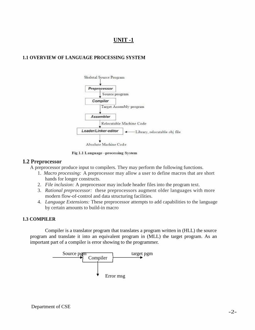
1.1 OVERVIEW OF LANGUAGE PROCESSING SYSTEM

1.2 Preprocessor

A preprocessor produce input to compilers. They may perform the following functions.

1. Macro processing: A preprocessor may allow a user to define macros that are short

hands for longer constructs.

2. File inclusion: A preprocessor may include header files into the program text.

3. Rational preprocessor: these preprocessors augment older languages with more

modern flow-of-control and data structuring facilities.

4. Language Extensions: These preprocessor attempts to add capabilities to the language

by certain amounts to build-in macro

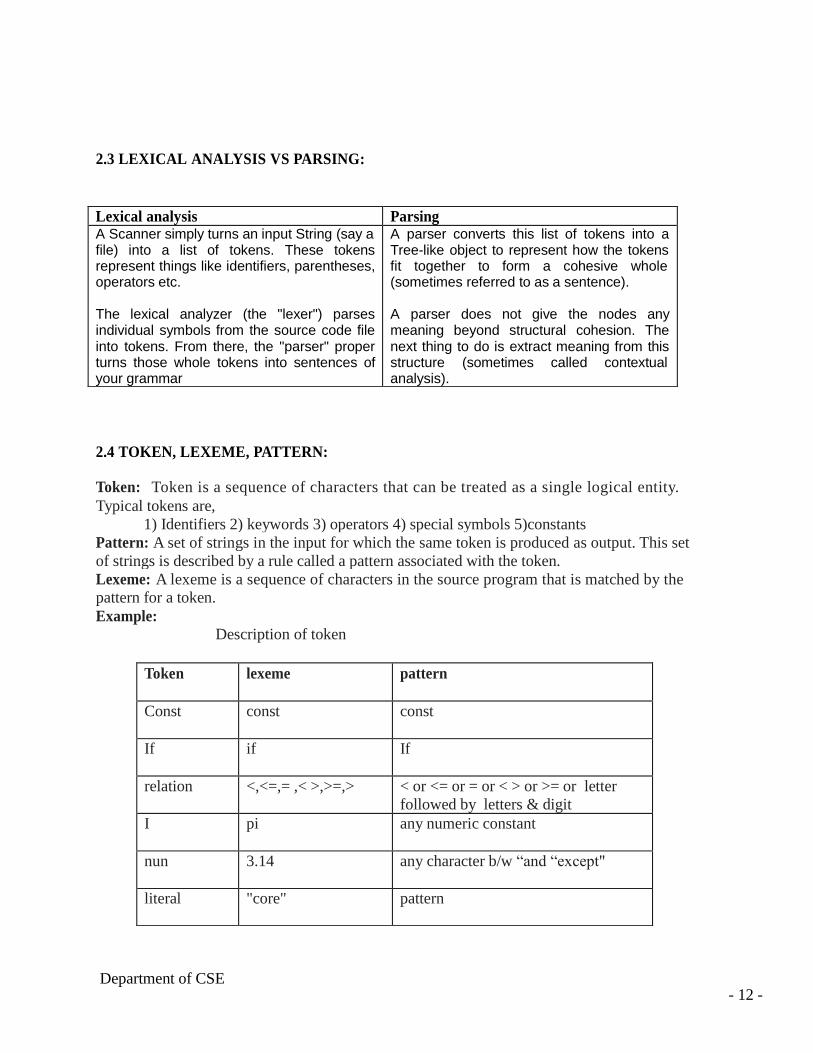
1.3 COMPILER

Compiler is a translator program that translates a program written in (HLL) the source

program and translate it into an equivalent program in (MLL) the target program. As an

important part of a compiler is error showing to the programmer.

Source pgm target pgm Compiler

Error msg


Obj pgm input opj pgm output

Executing a program written n HLL programming language is basically of two parts. the

source program must first be compiled translated into a object program. Then the results

object program is loaded into a memory executed.

Source pgm obj pgm Compiler

Obj pgm

1.4 ASSEMBLER: programmers found it difficult to write or read programs in machine

language. They begin to use a mnemonic (symbols) for each machine instruction, which

they would subsequently translate into machine language. Such a mnemonic machine

language is now called an assembly language. Programs known as assembler were

written to automate the translation of assembly language in to machine language. The

input to an assembler program is called source program, the output is a machine language

translation (object program).

1.5 INTERPRETER: An interpreter is a program that appears to execute a source

program as if it were machine language.

Languages such as BASIC, SNOBOL, LISP can be translated using interpreters. JAVA also

uses interpreter. The process of interpretation can be carried out in following phases.

1. Lexical analysis

2. Synatx analysis

3. Semantic analysis

4. Direct Execution

Advantages:

Modification of user program can be easily made and implemented as execution

proceeds.

Type of object that denotes a various may change dynamically.

Debugging a program and finding errors is simplified task for a program used for

interpretation.

The interpreter for the language makes it machine independent.

Department of CSE

-3-

Disadvantages:

The execution of the program is slower.

Memory consumption is more.

2 Loader and Link-editor:

Once the assembler procedures an object program, that program must be placed into

memory and executed. The assembler could place the object program directly in memory

and transfer control to it, thereby causing the machine language program to be

execute. This would waste core by leaving the assembler in memory while the user’s

program was being executed. Also the programmer would have to retranslate his program

with each execution, thus wasting translation time. To over come this problems of wasted

translation time and memory. System programmers developed another component called

loader

“A loader is a program that places programs into memory and prepares them for

execution.” It would be more efficient if subroutines could be translated into object form the

loader could”relocate” directly behind the user’s program. The task of adjusting programs o

they may be placed in arbitrary core locations is called relocation. Relocation loaders

perform four functions.

1.6 TRANSLATOR

A translator is a program that takes as input a program written in one language and

produces as output a program in another language. Beside program translation, the translator

performs another very important role, the error-detection. Any violation of d HLL

specification would be detected and reported to the programmers. Important role of translator

are:

1 Translating the hll program input into an equivalent ml program.

2 Providing diagnostic messages wherever the programmer violates specification of

the hll.

1.7 TYPE OF TRANSLATORS:-

INTERPRETOR

COMPILER

PREPROSSESSOR


1.8 LIST OF COMPILERS

1. Ada compilers

2 .ALGOL compilers

3 .BASIC compilers

4 .C# compilers

5 .C compilers

6 .C++ compilers

7 .COBOL compilers

8 .D compilers

9 .Common Lisp compilers

10. ECMAScript interpreters

11. Eiffel compilers

12. Felix compilers

13. Fortran compilers

14. Haskell compilers

15 .Java compilers

16. Pascal compilers

17. PL/I compilers

18. Python compilers

19. Scheme compilers

20. Smalltalk compilers

21. CIL compilers

1.9 STRUCTURE OF THE COMPILER DESIGN

Phases of a compiler: A compiler operates in phases. A phase is a logically interrelated

operation that takes source program in one representation and produces output in another

representation. The phases of a compiler are shown in below

There are two phases of compilation.

a. Analysis (Machine Independent/Language Dependent)

b. Synthesis(Machine Dependent/Language independent)

Compilation process is partitioned into no-of-sub processes called ‘phases’.

Department of CSE

-5-

Lexical Analysis:-

LA or Scanners reads the source program one character at a time, carving the

source program into a sequence of automic units called tokens.

Syntax Analysis:-

The second stage of translation is called Syntax analysis or parsing. In this

phase expressions, statements, declarations etc… are identified by using the results of lexical

analysis. Syntax analysis is aided by using techniques based on formal grammar of the

programming language.

Intermediate Code Generations:-

An intermediate representation of the final machine language code is produced.

This phase bridges the analysis and synthesis phases of translation.

Code Optimization :-

This is optional phase described to improve the intermediate code so that the

output runs faster and takes less space.

Code Generation:-

The last phase of translation is code generation. A number of optimizations to

reduce the length of machine language program are carried out during this phase. The

output of the code generator is the machine language program of the specified computer.

Table Management (or) Book-keeping:-

Department of CSE

-6-

This is the portion to keep the names used by the program and records

essential information about each. The data structure used to record this information called a

‘Symbol Table’. Error Handlers:-

It is invoked when a flaw error in the source program is detected.

The output of LA is a stream of tokens, which is passed to the next phase, the

syntax analyzer or parser. The SA groups the tokens together into syntactic structure called

as expression. Expression may further be combined to form statements. The syntactic

structure can be regarded as a tree whose leaves are the token called as parse trees.

The parser has two functions. It checks if the tokens from lexical analyzer,

occur in pattern that are permitted by the specification for the source language. It also

imposes on tokens a tree-like structure that is used by the sub-sequent phases of the compiler.

Example, if a program contains the expression A+/B after lexical analysis this

expression might appear to the syntax analyzer as the token sequence id+/id. On seeing the /, the syntax analyzer should detect an error situation, because the presence of these two

adjacent binary operators violates the formulations rule of an expression.

Syntax analysis is to make explicit the hierarchical structure of the incoming

token stream by identifying which parts of the token stream should be grouped.

Example, (A/B*C has two possible interpretations.)

1, divide A by B and then multiply by C or

2, multiply B by C and then use the result to divide A.

each of these two interpretations can be represented in terms of a parse tree.

Intermediate Code Generation:-

The intermediate code generation uses the structure produced by the syntax

analyzer to create a stream of simple instructions. Many styles of intermediate code are

possible. One common style uses instruction with one operator and a small number of

operands.

The output of the syntax analyzer is some representation of a parse tree. the

intermediate code generation phase transforms this parse tree into an intermediate language

representation of the source program.

Code Optimization

This is optional phase described to improve the intermediate code so that the

output runs faster and takes less space. Its output is another intermediate code program that

does the some job as the original, but in a way that saves time and / or spaces.

1, Local Optimization:-

There are local transformations that can be applied to a program to

make an improvement. For example,

If A > B goto L2


Goto L3

L2 :

This can be replaced by a single statement

If A < B goto L3

Another important local optimization is the elimination of common

sub-expressions

A := B + C + D

E := B + C + F

Might be evaluated as

T1 := B + C

A := T1 + D

E := T1 + F

Take this advantage of the common sub-expressions B + C.

2, Loop Optimization:-

Another important source of optimization concerns about increasing

the speed of loops. A typical loop improvement is to move a

computation that produces the same result each time around the loop

to a point, in the program just before the loop is entered.

Code generator :-

Cg produces the object code by deciding on the memory locations for data,

selecting code to access each datum and selecting the registers in which each computation is

to be done. Many computers have only a few high speed registers in which computations can

be performed quickly. A good code generator would attempt to utilize registers as efficiently

as possible.

Table Management OR Book-keeping :-

A compiler needs to collect information about all the data objects that appear

in the source program. The information about data objects is collected by the early phases of

the compiler-lexical and syntactic analyzers. The data structure used to record this

information is called as Symbol Table.

Error Handing :-

One of the most important functions of a compiler is the detection and

reporting of errors in the source program. The error message should allow the programmer to

determine exactly where the errors have occurred. Errors may occur in all or the phases of a

compiler.

Whenever a phase of the compiler discovers an error, it must report the error to

the error handler, which issues an appropriate diagnostic msg. Both of the table-management

and error-Handling routines interact with all phases of the compiler.

Department of CSE

-8-

Example:

Position:= initial + rate *60

Lexical Analyzer

Tokens id1 = id2 + id3 * id4

Syntsx Analyzer

=

id1 +

id2 *

id3 id4

Semantic Analyzer

=

id1 +

id2 *

id3 60

int to real

Intermediate Code Generator

temp1:= int to real (60)

temp2:= id3 * temp1

temp3:= id2 + temp2

id1:= temp3.

Code Optimizer

Temp1:= id3 * 60.0


Id1:= id2 +temp1

Code Generator

MOVF id3, r2

MULF *60.0, r2

MOVF id2, r2

ADDF r2, r1

MOVF r1, id1

1.10 TOKEN

LA reads the source program one character at a time, carving the source program into

a sequence of automatic units called ‘Tokens’. 1, Type of the token.

2, Value of the token.

Type : variable, operator, keyword, constant

Value : N1ame of variable, current variable (or) pointer to symbol table.

If the symbols given in the standard format the LA accepts and produces

token as output. Each token is a sub-string of the program that is to be treated as a single

unit. Token are two types.

1, Specific strings such as IF (or) semicolon.

2, Classes of string such as identifiers, label, constants.

Department of CSE - 10 -

UNIT -2

LEXICAL ANALYSIS

2.1 OVER VIEW OF LEXICAL ANALYSIS

o To identify the tokens we need some method of describing the possible tokens

that can appear in the input stream. For this purpose we introduce regular expression, a

notation that can be used to describe essentially all the tokens of programming

language.

o Secondly , having decided what the tokens are, we need some mechanism to

recognize these in the input stream. This is done by the token recognizers, which are

designed using transition diagrams and finite automata.

2.2 ROLE OF LEXICAL ANALYZER

the LA is the first phase of a compiler. It main task is to read the input character

and produce as output a sequence of tokens that the parser uses for syntax analysis.

Upon receiving a ‘get next token’ command form the parser, the lexical analyzer

reads the input character until it can identify the next token. The LA return to the parser

representation for the token it has found. The representation will be an integer code, if the

token is a simple construct such as parenthesis, comma or colon.

LA may also perform certain secondary tasks as the user interface. One such task is

striping out from the source program the commands and white spaces in the form of blank,

tab and new line characters. Another is correlating error message from the compiler with the

source program.

Department of CSE

- 11 -

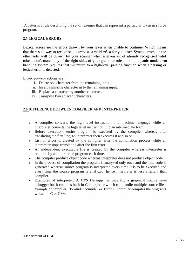
2.3 LEXICAL ANALYSIS VS PARSING:

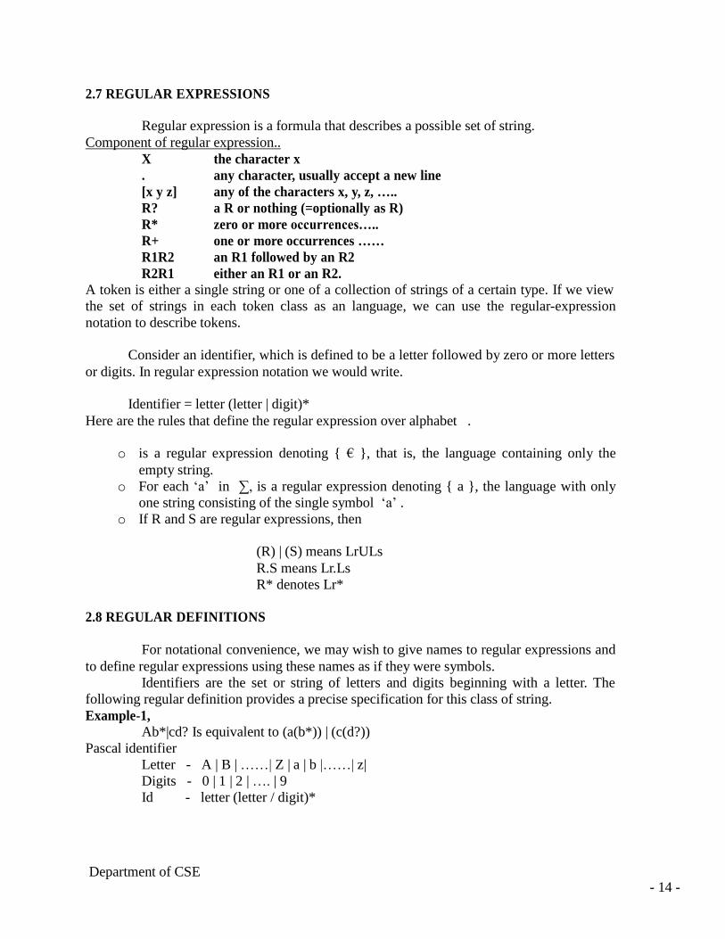
2.4 TOKEN, LEXEME, PATTERN:

Token: Token is a sequence of characters that can be treated as a single logical entity.

Typical tokens are,

1) Identifiers 2) keywords 3) operators 4) special symbols 5)constants

Pattern: A set of strings in the input for which the same token is produced as output. This set

of strings is described by a rule called a pattern associated with the token.

Lexeme: A lexeme is a sequence of characters in the source program that is matched by the

pattern for a token.

Example:

Description of token

Department of CSE

- 12 -

Token lexeme pattern

Const const const

If if If

relation <,<=,= ,< >,>=,> < or <= or = or < > or >= or letter

followed by letters & digit

I pi any numeric constant

nun 3.14 any character b/w “and “except"

literal "core" pattern

Lexical analysis Parsing A Scanner simply turns an input String (say a file) into a list of tokens. These tokens represent things like identifiers, parentheses, operators etc. The lexical analyzer (the "lexer") parses individual symbols from the source code file into tokens. From there, the "parser" proper turns those whole tokens into sentences of your grammar

A parser converts this list of tokens into a Tree-like object to represent how the tokens fit together to form a cohesive whole (sometimes referred to as a sentence). A parser does not give the nodes any meaning beyond structural cohesion. The next thing to do is extract meaning from this structure (sometimes called contextual analysis).

A patter is a rule describing the set of lexemes that can represent a particular token in source

program.

2.5 LEXICAL ERRORS:

Lexical errors are the errors thrown by your lexer when unable to continue. Which means

that there's no way to recognise a lexeme as a valid token for you lexer. Syntax errors, on the

other side, will be thrown by your scanner when a given set of already recognised valid

tokens don't match any of the right sides of your grammar rules. simple panic-mode error

handling system requires that we return to a high-level parsing function when a parsing or

lexical error is detected.

Error-recovery actions are:

i. Delete one character from the remaining input.

ii. Insert a missing character in to the remaining input.

iii. Replace a character by another character.

iv. Transpose two adjacent characters.

2.6 DIFFERENCE BETWEEN COMPILER AND INTERPRETER

A compiler converts the high level instruction into machine language while an

interpreter converts the high level instruction into an intermediate form.

Before execution, entire program is executed by the compiler whereas after

translating the first line, an interpreter then executes it and so on.

List of errors is created by the compiler after the compilation process while an

interpreter stops translating after the first error.

An independent executable file is created by the compiler whereas interpreter is

required by an interpreted program each time.

The compiler produce object code whereas interpreter does not produce object code.

In the process of compilation the program is analyzed only once and then the code is

generated whereas source program is interpreted every time it is to be executed and

every time the source program is analyzed. hence interpreter is less efficient than

compiler.

Examples of interpreter: A UPS Debugger is basically a graphical source level

debugger but it contains built in C interpreter which can handle multiple source files.

example of compiler: Borland c compiler or Turbo C compiler compiles the programs

written in C or C++.


2.7 REGULAR EXPRESSIONS

Regular expression is a formula that describes a possible set of string.

Component of regular expression..

X the character x

. any character, usually accept a new line

[x y z] any of the characters x, y, z, …..

R? a R or nothing (=optionally as R)

R* zero or more occurrences…..

R+ one or more occurrences ……

R1R2 an R1 followed by an R2

R2R1 either an R1 or an R2.

A token is either a single string or one of a collection of strings of a certain type. If we view

the set of strings in each token class as an language, we can use the regular-expression

notation to describe tokens.

Consider an identifier, which is defined to be a letter followed by zero or more letters

or digits. In regular expression notation we would write.

Identifier = letter (letter | digit)*

Here are the rules that define the regular expression over alphabet .

o is a regular expression denoting { € }, that is, the language containing only the

empty string.

o For each ‘a’ in ∑, is a regular expression denoting { a }, the language with only

one string consisting of the single symbol ‘a’ . o If R and S are regular expressions, then

(R) | (S) means LrULs

R.S means Lr.Ls

R* denotes Lr*

2.8 REGULAR DEFINITIONS

For notational convenience, we may wish to give names to regular expressions and

to define regular expressions using these names as if they were symbols.

Identifiers are the set or string of letters and digits beginning with a letter. The

following regular definition provides a precise specification for this class of string.

Example-1,

Ab*|cd? Is equivalent to (a(b*)) | (c(d?))

Pascal identifier

Letter - A | B | ……| Z | a | b |……| z|

Digits - 0 | 1 | 2 | …. | 9

Id - letter (letter / digit)*


parser.

Recognition of tokens:

We learn how to express pattern using regular expressions. Now, we must study how to take

the patterns for all the needed tokens and build a piece of code that examins the input string

and finds a prefix that is a lexeme matching one of the

patterns.

Stmt if expr then stmt

| If expr then else stmt

| є

Expr term relop term

| term

Term id

|number

For relop ,we use the comparison operations of languages like Pascal or SQL where = is

“equals” and < > is “not equals” because it presents an interesting structure of lexemes.

The terminal of grammar, which are if, then , else, relop ,id and numbers are the names of

tokens as far as the lexical analyzer is concerned, the patterns for the tokens are described

using regular definitions.

digit -->[0,9]

digits -->digit+

number -->digit(.digit)?(e.[+-]?digits)?

letter -->[A-Z,a-z]

id -->letter(letter/digit)*

if --> if

then -->then

else -->else

relop --></>/<=/>=/==/< >

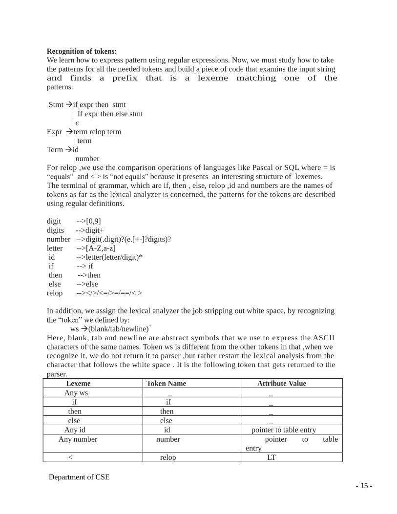
In addition, we assign the lexical analyzer the job stripping out white space, by recognizing

the “token” we defined by:

ws (blank/tab/newline)+

Here, blank, tab and newline are abstract symbols that we use to express the ASCII

characters of the same names. Token ws is different from the other tokens in that ,when we

recognize it, we do not return it to parser ,but rather restart the lexical analysis from the

character that follows the white space . It is the following token that gets returned to the

Department of CSE

- 15 -

Lexeme Token Name Attribute Value

Any ws _ _

if if _

then then _

else else _

Any id id pointer to table entry

Any number number pointer to table

entry

< relop LT

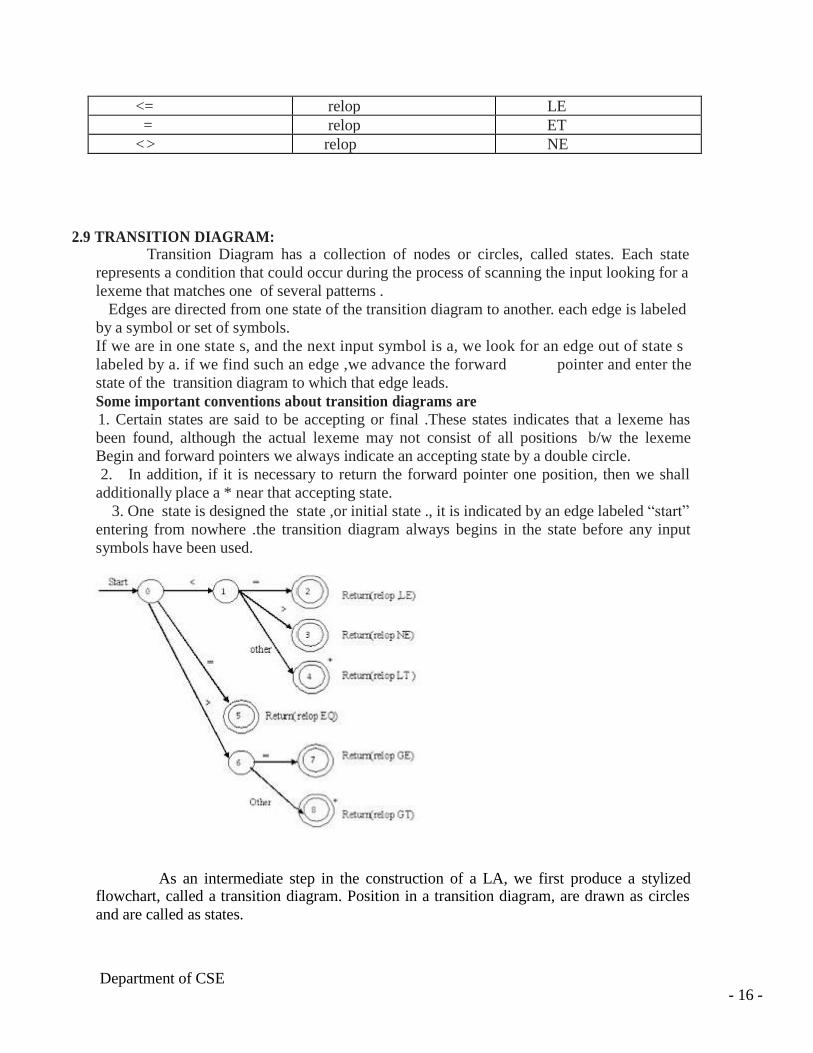
2.9 TRANSITION DIAGRAM:

Transition Diagram has a collection of nodes or circles, called states. Each state

represents a condition that could occur during the process of scanning the input looking for a

lexeme that matches one of several patterns . Edges are directed from one state of the transition diagram to another. each edge is labeled

by a symbol or set of symbols.

If we are in one state s, and the next input symbol is a, we look for an edge out of state s

labeled by a. if we find such an edge ,we advance the forward pointer and enter the

state of the transition diagram to which that edge leads.

Some important conventions about transition diagrams are

1. Certain states are said to be accepting or final .These states indicates that a lexeme has

been found, although the actual lexeme may not consist of all positions b/w the lexeme

Begin and forward pointers we always indicate an accepting state by a double circle.

2. In addition, if it is necessary to return the forward pointer one position, then we shall

additionally place a * near that accepting state.

3. One state is designed the state ,or initial state ., it is indicated by an edge labeled “start”

entering from nowhere .the transition diagram always begins in the state before any input

symbols have been used.

As an intermediate step in the construction of a LA, we first produce a stylized

flowchart, called a transition diagram. Position in a transition diagram, are drawn as circles

and are called as states. Department of CSE

- 16 -

<= relop LE

= relop ET

<> relop NE

The above TD for an identifier, defined to be a letter followed by any no of letters

or digits.A sequence of transition diagram can be converted into program to look for the

tokens specified by the diagrams. Each state gets a segment of code.

If = if

Then = then

Else = else

Relop = < | <= | = | > | >=

Id = letter (letter | digit) *|

Num = digit | 2.10 AUTOMATA

An automation is defined as a system where information is transmitted and used for

performing some functions without direct participation of man.

1, an automation in which the output depends only on the input is called an

automation without memory.

2, an automation in which the output depends on the input and state also is called as

automation with memory.

3, an automation in which the output depends only on the state of the machine is

called a Moore machine.

3, an automation in which the output depends on the state and input at any instant of

time is called a mealy machine.

2.11 DESCRIPTION OF AUTOMATA

1, an automata has a mechanism to read input from input tape,

2, any language is recognized by some automation, Hence these automation are

basically language ‘acceptors’ or ‘language recognizers’. Types of Finite Automata

Deterministic Automata

Non-Deterministic Automata.

2.12 DETERMINISTIC AUTOMATA

A deterministic finite automata has at most one transition from each state on any

input. A DFA is a special case of a NFA in which:-

1, it has no transitions on input € ,

Department of CSE

- 17 -

2, each input symbol has at most one transition from any state.

DFA formally defined by 5 tuple notation M = (Q, ∑, δ, qo, F), where

Q is a finite ‘set of states’, which is non empty.

∑ is ‘input alphabets’, indicates input set.

qo is an ‘initial state’ and qo is in Q ie, qo, ∑, Q

F is a set of ‘Final states’, δ is a ‘transmission function’ or mapping function, using this function the

next state can be determined.

The regular expression is converted into minimized DFA by the following procedure:

Regular expression → NFA → DFA → Minimized DFA

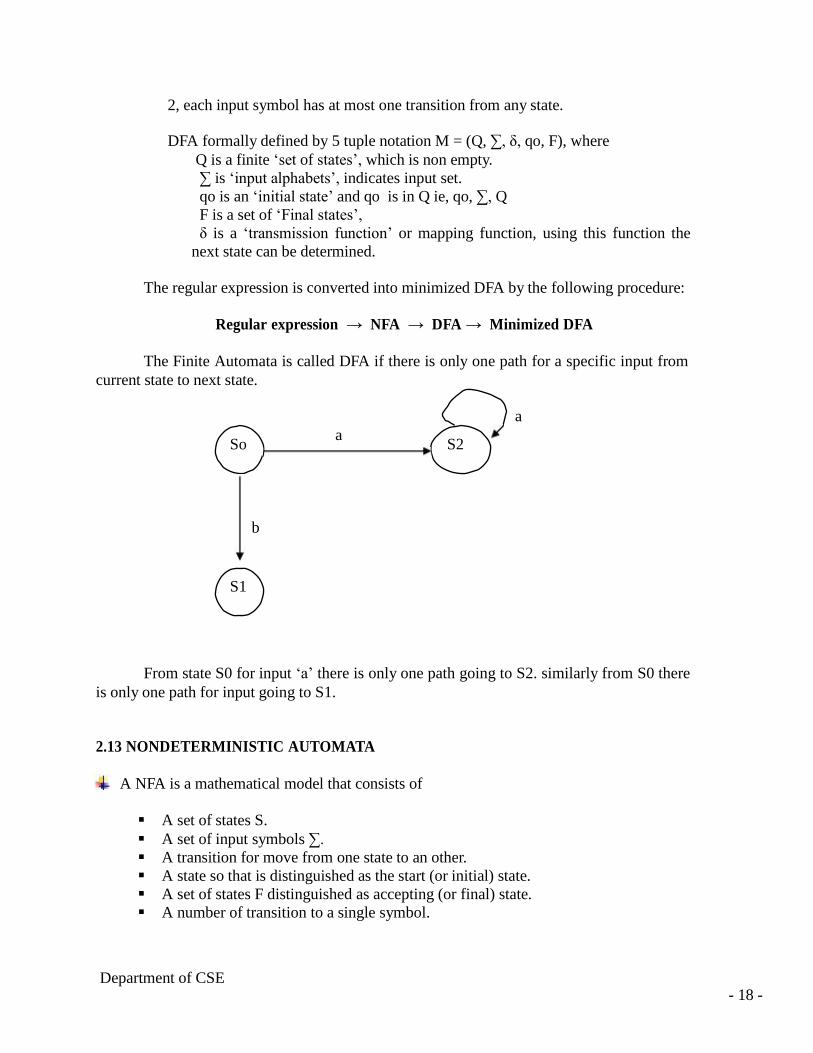
The Finite Automata is called DFA if there is only one path for a specific input from

current state to next state.

a

So a

S2

b

S1

From state S0 for input ‘a’ there is only one path going to S2. similarly from S0 there

is only one path for input going to S1.

2.13 NONDETERMINISTIC AUTOMATA

A NFA is a mathematical model that consists of

A set of states S.

A set of input symbols ∑. A transition for move from one state to an other.

A state so that is distinguished as the start (or initial) state.

A set of states F distinguished as accepting (or final) state.

A number of transition to a single symbol.


A NFA can be diagrammatically represented by a labeled directed graph, called a

transition graph, In which the nodes are the states and the labeled edges represent

the transition function.

This graph looks like a transition diagram, but the same character can label two or

more transitions out of one state and edges can be labeled by the special symbol €

as well as by input symbols.

The transition graph for an NFA that recognizes the language ( a | b ) * abb is

shown

2.14 DEFINITION OF CFG

It involves four quantities.

CFG contain terminals, N-T, start symbol and production.

Terminal are basic symbols form which string are formed.

N-terminals are synthetic variables that denote sets of strings

In a Grammar, one N-T are distinguished as the start symbol, and the set of

string it denotes is the language defined by the grammar.

The production of the grammar specify the manor in which the terminal and

N-T can be combined to form strings.

Each production consists of a N-T, followed by an arrow, followed by a string

of one terminal and terminals.

2.15 DEFINITION OF SYMBOL TABLE

An extensible array of records.

The identifier and the associated records contains collected information about

the identifier.

FUNCTION identify (Identifier name)

RETURNING a pointer to identifier information contains

The actual string

A macro definition

A keyword definition

A list of type, variable & function definition

A list of structure and union name definition

A list of structure and union field selected definitions.

Department of CSE

- 19 -

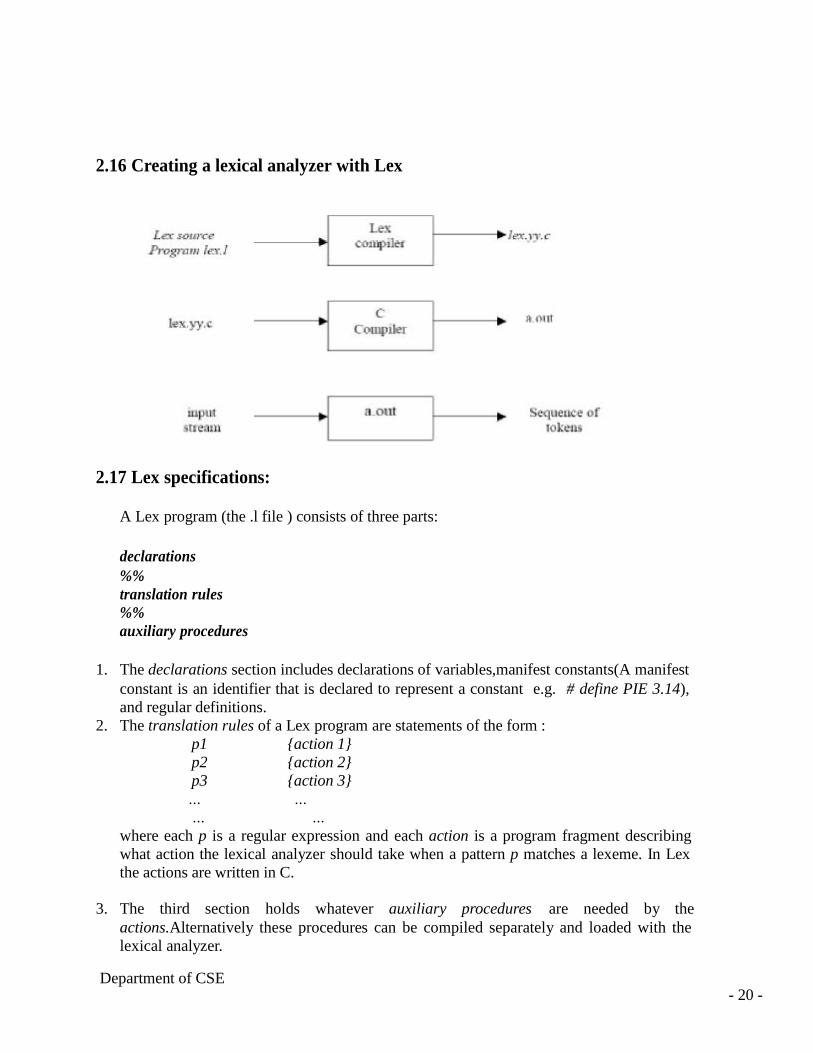
2.16 Creating a lexical analyzer with Lex

2.17 Lex specifications:

A Lex program (the .l file ) consists of three parts:

declarations

%%

translation rules

%%

auxiliary procedures

1. The declarations section includes declarations of variables,manifest constants(A manifest

constant is an identifier that is declared to represent a constant e.g. # define PIE 3.14),

and regular definitions.

2. The translation rules of a Lex program are statements of the form : p1 {action 1}

p2 {action 2}

p3 {action 3}

… …

… …

where each p is a regular expression and each action is a program fragment describing

what action the lexical analyzer should take when a pattern p matches a lexeme. In Lex

the actions are written in C.

3. The third section holds whatever auxiliary procedures are needed by the

actions.Alternatively these procedures can be compiled separately and loaded with the

lexical analyzer.


Note: You can refer to a sample lex program given in page no. 109 of chapter 3 of the book:

Compilers: Principles, Techniques, and Tools by Aho, Sethi & Ullman for more clarity.

2.18 INPUT BUFFERING

The LA scans the characters of the source pgm one at a time to discover tokens.

Because of large amount of time can be consumed scanning characters, specialized buffering

techniques have been developed to reduce the amount of overhead required to process an

input character.

Buffering techniques:

1. Buffer pairs

2. Sentinels

The lexical analyzer scans the characters of the source program one a t a time to discover

tokens. Often, however, many characters beyond the next token many have to be examined

before the next token itself can be determined. For this and other reasons, it is desirable for

thelexical analyzer to read its input from an input buffer. Figure shows a buffer divided into

two haves of, say 100 characters each. One pointer marks the beginning of the token being

discovered. A look ahead pointer scans ahead of the beginning point, until the token is

discovered .we view the position of each pointer as being between the character last read and

thecharacter next to be read. In practice each buffering scheme adopts one convention either

apointer is at the symbol last read or the symbol it is ready to read.

Token beginnings look ahead pointerThe distance which the lookahead pointer may

have to travel past the actual token may belarge. For example, in a PL/I program we may see:

DECALRE (ARG1, ARG2… ARG n) Without knowing whether DECLARE is a keyword or

an array name until we see the character that follows the right parenthesis. In either case, the

token itself ends at the second E. If the look ahead pointer travels beyond the buffer half in

which it began, the other half must be loaded with the next characters from the source file.

Since the buffer shown in above figure is of limited size there is an implied constraint on

how much look ahead can be used before the next token is discovered. In the above example,

ifthe look ahead traveled to the left half and all the way through the left half to the middle,

we could not reload the right half, because we would lose characters that had not yet been

groupedinto tokens. While we can make the buffer larger if we chose or use another

buffering scheme,we cannot ignore the fact that overhead is limited.

Department of CSE

- 21 -

UNIT -3

SYNTAX ANALYSIS

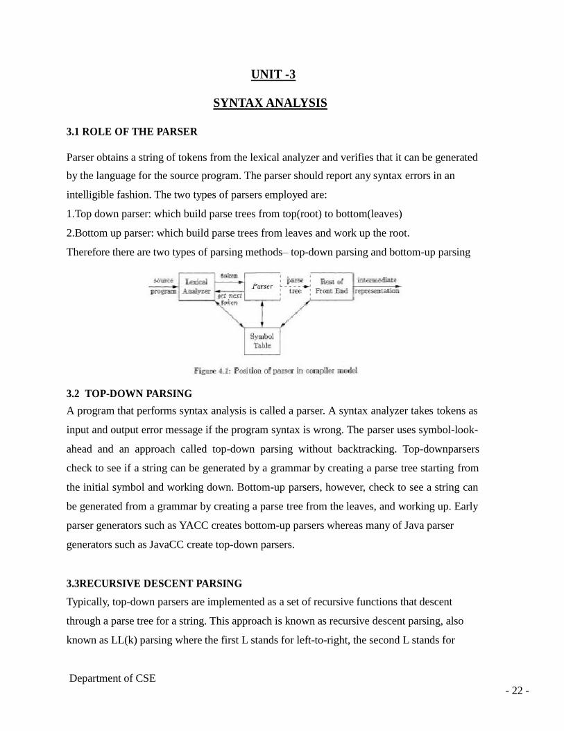
3.1 ROLE OF THE PARSER

Parser obtains a string of tokens from the lexical analyzer and verifies that it can be generated

by the language for the source program. The parser should report any syntax errors in an

intelligible fashion. The two types of parsers employed are:

1.Top down parser: which build parse trees from top(root) to bottom(leaves)

2.Bottom up parser: which build parse trees from leaves and work up the root.

Therefore there are two types of parsing methods– top-down parsing and bottom-up parsing

3.2 TOP-DOWN PARSING

A program that performs syntax analysis is called a parser. A syntax analyzer takes tokens as

input and output error message if the program syntax is wrong. The parser uses symbol-look-

ahead and an approach called top-down parsing without backtracking. Top-downparsers

check to see if a string can be generated by a grammar by creating a parse tree starting from

the initial symbol and working down. Bottom-up parsers, however, check to see a string can

be generated from a grammar by creating a parse tree from the leaves, and working up. Early

parser generators such as YACC creates bottom-up parsers whereas many of Java parser

generators such as JavaCC create top-down parsers.

3.3RECURSIVE DESCENT PARSING

Typically, top-down parsers are implemented as a set of recursive functions that descent

through a parse tree for a string. This approach is known as recursive descent parsing, also

known as LL(k) parsing where the first L stands for left-to-right, the second L stands for

Department of CSE

- 22 -

leftmost-derivation, and k indicates k-symbol lookahead. Therefore, a parser using the single

symbol look-ahead method and top-down parsing without backtracking is called LL(1)

parser. In the following sections, we will also use an extended BNF notation in which some

regulation expression operators are to be incorporated.

A syntax expression defines sentences of the form , or . A syntax of the form defines

sentences that consist of a sentence of the form followed by a sentence of the form followed

by a sentence of the form . A syntax of the form defines zero or one occurrence of the form .

A syntax of the form defines zero or more occurrences of the form .

A usual implementation of an LL(1) parser is:

o initialize its data structures,

o get the lookahead token by calling scanner routines, and

o call the routine that implements the start symbol.

Here is an example.

proc syntaxAnalysis()

begin

initialize(); // initialize global data and structures

nextToken(); // get the lookahead token

program(); // parser routine that implements the start symbol

end;

3.4 FIRST AND FOLLOW

To compute FIRST(X) for all grammar symbols X, apply the following rules until

no more terminals or e can be added to any FIRST set.

1. If X is terminal, then FIRST(X) is {X}.

2. If X->e is a production, then add e to FIRST(X).

3. If X is nonterminal and X->Y1Y2...Yk is a production, then place a in FIRST(X) if for

some i, a is in FIRST(Yi) and e is in all of FIRST(Y1),...,FIRST(Yi-1) that is,

Y1...... Yi-1=*>e.If e is in FIRST(Yj) for all j=1,2,...,k, then add e to FIRST(X). For

example, everything in FIRST(Yj) is surely in FIRST(X). If y1 does not derive e, then we

add nothing more to FIRST(X), but if Y1=*>e, then we add FIRST(Y2) and so on.

Department of CSE

- 23 -

To compute the FIRST(A) for all nonterminals A, apply the following rules until nothing

can be added to any FOLLOW set.

1. Place $ in FOLLOW(S), where S is the start symbol and $ in the input right endmarker.

2. If there is a production A=>aBs where FIRST(s) except e is placed in FOLLOW(B).

3. If there is aproduction A->aB or a production A->aBs where FIRST(s) contains e, then

everything in FOLLOW(A) is in FOLLOW(B).

Consider the following example to understand the concept of First and Follow.Find the first

and follow of all nonterminals in the Grammar-

E -> TE'

E'-> +TE'|e

T -> FT'

T'-> *FT'|e

F -> (E)|id

Then:

FIRST(E)=FIRST(T)=FIRST(F)={(,id}

FIRST(E')={+,e}

FIRST(T')={*,e}

FOLLOW(E)=FOLLOW(E')={),$}

FOLLOW(T)=FOLLOW(T')={+,),$}

FOLLOW(F)={+,*,),$}

For example, id and left parenthesis are added to FIRST(F) by rule 3 in definition of FIRST

with i=1 in each case, since FIRST(id)=(id) and FIRST('(')= {(} by rule 1. Then by rule 3

with i=1, the production T -> FT' implies that id and left parenthesis belong to FIRST(T)

also.

To compute FOLLOW,we put $ in FOLLOW(E) by rule 1 for FOLLOW. By rule 2 applied

toproduction F-> (E), right parenthesis is also in FOLLOW(E). By rule 3 applied to

production E-> TE', $ and right parenthesis are in FOLLOW(E').


3.5 CONSTRUCTION OF PREDICTIVE PARSING TABLES

For any grammar G, the following algorithm can be used to construct the predictive parsing

table. The algorithm is

Input : Grammar G

Output : Parsing table M

Method

1. 1.For each production A-> a of the grammar, do steps 2 and 3.

2. For each terminal a in FIRST(a), add A->a, to M[A,a].

3. If e is in First(a), add A->a to M[A,b] for each terminal b in FOLLOW(A). If e is in

FIRST(a) and $ is in FOLLOW(A), add A->a to M[A,$].

4. Make each undefined entry of M be error.

3.6.LL(1) GRAMMAR

The above algorithm can be applied to any grammar G to produce a parsing table M. For

some Grammars, for example if G is left recursive or ambiguous, then M will have at least

one multiply-defined entry. A grammar whose parsing table has no multiply defined entries

is said to be LL(1). It can be shown that the above algorithm can be used to produce for every

LL(1) grammar G a parsing table M that parses all and only the sentences of G. LL(1)

grammars have several distinctive properties. No ambiguous or left recursive grammar can

be LL(1). There remains a question of what should be done in case of multiply defined

entries. One easy solution is to eliminate all left recursion and left factoring, hoping to

produce a grammar which will produce no multiply defined entries in the parse tables.

Unfortunately there are some grammars which will give an LL(1) grammar after any kind of

alteration. In general, there are no universal rules to convert multiply defined entries into

single valued entries without affecting the language recognized by the parser.

The main difficulty in using predictive parsing is in writing a grammar for the source

language such that a predictive parser can be constructed from the grammar. Although left

recursion elimination and left factoring are easy to do, they make the resulting grammar hard

to read and difficult to use the translation purposes. To alleviate some of this difficulty, a

common organization for a parser in a compiler is to use a predictive parser for control

Department of CSE

- 25 -

constructs and to use operator precedence for expressions.however, if an lr parser generator

is available, one can get all the benefits of predictive parsing and operator precedence

automatically.

3.7.ERROR RECOVERY IN PREDICTIVE PARSING

The stack of a nonrecursive predictive parser makes explicit the terminals and nonterminals

that the parser hopes to match with the remainder of the input. We shall therefore refer to

symbols on the parser stack in the following discussion. An error is detected during

predictive parsing when the terminal on top of the stack does not match the next input

symbol or when nonterminal A is on top of the stack, a is the next input symbol, and the

parsing table entry M[A,a] is empty.

Panic-mode error recovery is based on the idea of skipping symbols on the input until a token

in a selected set of synchronizing tokens appears. Its effectiveness depends on the choice of

synchronizing set. The sets should be chosen so that the parser recovers quickly from errors

that are likely to occur in practice. Some heuristics are as follows

As a starting point, we can place all symbols in FOLLOW(A) into the synchronizing

set for nonterminal A. If we skip tokens until an element of FOLLOW(A) is seen and

pop A from the stack, it is likely that parsing can continue.

It is not enough to use FOLLOW(A) as the synchronizingset for A. Fo example , if

semicolons terminate statements, as in C, then keywords that begin statements may

not appear in the FOLLOW set of the nonterminal generating expressions. A missing

semicolon after an assignment may therefore result in the keyword beginning the next

statement being skipped. Often, there is a hierarchica structure on constructs in a

language; e.g., expressions appear within statement, which appear within bblocks,and

so on. We can add to the synchronizing set of a lower construct the symbols that

begin higher constructs. For example, we might add keywords that begin statements

to the synchronizing sets for the nonterminals generaitn expressions.

If we add symbols in FIRST(A) to the synchronizing set for nonterminal A, then it

may be possible to resume parsing according to A if a symbol in FIRST(A) appears in

the input.

Department of CSE

- 26 -

If a nonterminal can generate the empty string, then the production deriving e can be

used as a default. Doing so may postpone some error detection, but cannot cause an

error to be missed. This approach reduces the number of nonterminals that have to be

considered during error recovery.

If a terminal on top of the stack cannot be matched, a simple idea is to pop the

terminal, issue a message saying that the terminal was inserted, and continue parsing.

In effect, this approach takes the synchronizing set of a token to consist of all other

tokens.

Department of CSE

- 27 -

UNIT 4

LR PARSER

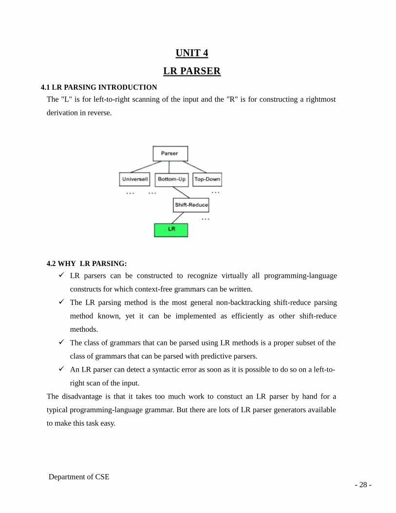
4.1 LR PARSING INTRODUCTION

The "L" is for left-to-right scanning of the input and the "R" is for constructing a rightmost

derivation in reverse.

4.2 WHY LR PARSING:

LR parsers can be constructed to recognize virtually all programming-language

constructs for which context-free grammars can be written.

The LR parsing method is the most general non-backtracking shift-reduce parsing

method known, yet it can be implemented as efficiently as other shift-reduce

methods.

The class of grammars that can be parsed using LR methods is a proper subset of the

class of grammars that can be parsed with predictive parsers.

An LR parser can detect a syntactic error as soon as it is possible to do so on a left-to-

right scan of the input.

The disadvantage is that it takes too much work to constuct an LR parser by hand for a

typical programming-language grammar. But there are lots of LR parser generators available

to make this task easy.

Department of CSE

- 28 -

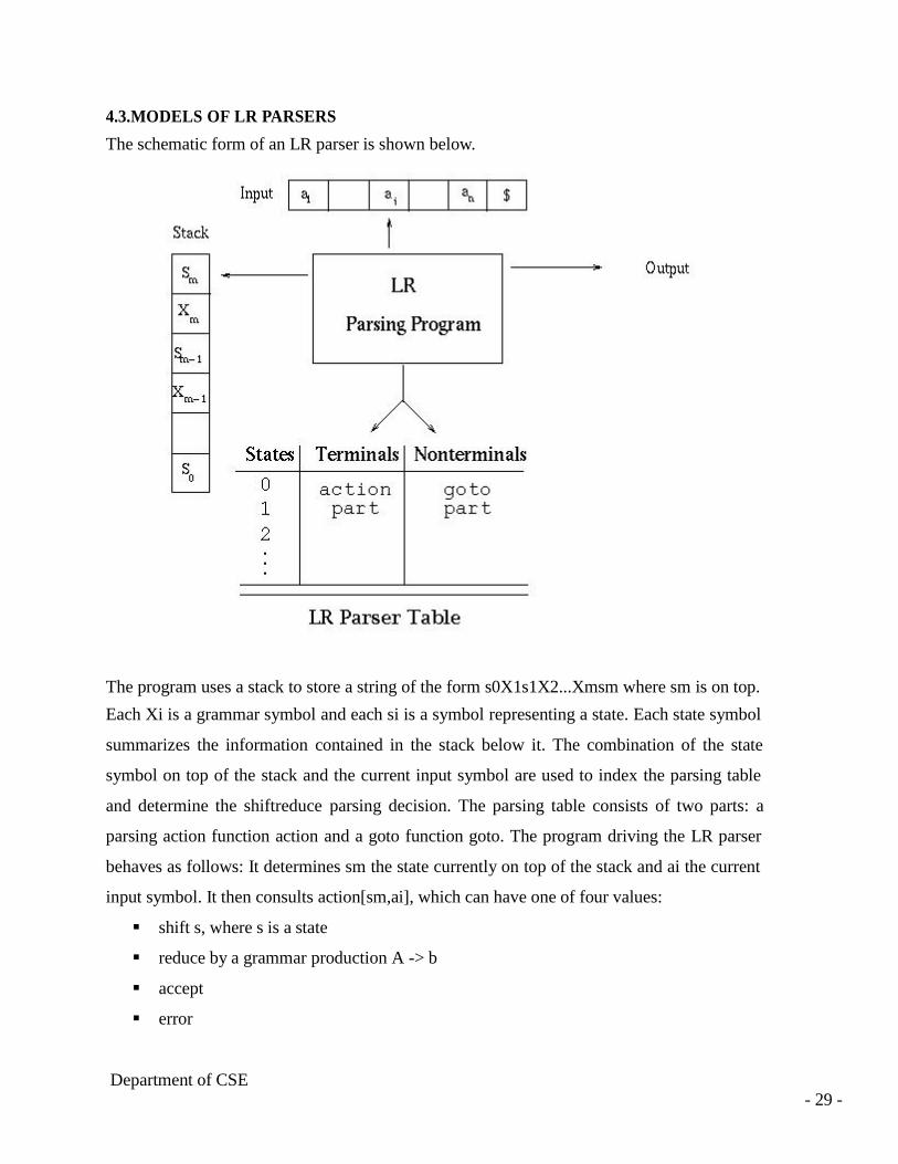
4.3.MODELS OF LR PARSERS

The schematic form of an LR parser is shown below.

The program uses a stack to store a string of the form s0X1s1X2...Xmsm where sm is on top.

Each Xi is a grammar symbol and each si is a symbol representing a state. Each state symbol

summarizes the information contained in the stack below it. The combination of the state

symbol on top of the stack and the current input symbol are used to index the parsing table

and determine the shiftreduce parsing decision. The parsing table consists of two parts: a

parsing action function action and a goto function goto. The program driving the LR parser

behaves as follows: It determines sm the state currently on top of the stack and ai the current

input symbol. It then consults action[sm,ai], which can have one of four values:

shift s, where s is a state

reduce by a grammar production A -> b

accept

error

Department of CSE

- 29 -

The function goto takes a state and grammar symbol as arguments and produces a state.

For a parsing table constructed for a grammar G, the goto table is the transition function of a

deterministic finite automaton that recognizes the viable prefixes of G. Recall that the viable

prefixes of G are those prefixes of right-sentential forms that can appear on the stack of a

shiftreduce parser because they do not extend past the rightmost handle.

A configuration of an LR parser is a pair whose first component is the stack contents and

whose second component is the unexpended input:

(s0 X1 s1 X2 s2... Xm sm, ai ai+1... an$)

This configuration represents the right-sentential form

X1 X1 ... Xm ai ai+1 ...an

in essentially the same way a shift-reduce parser would; only the presence of the states on the

stack is new. Recall the sample parse we did (see Example 1: Sample bottom-up parse) in

which we assembled the right-sentential form by concatenating the remainder of the input

buffer to the top of the stack. The next move of the parser is determined by reading ai and

sm, and consulting the parsing action table entry action[sm, ai]. Note that we are just looking

at the state here and no symbol below it. We'll see how this actually works later.

The configurations resulting after each of the four types of move are as follows:

If action[sm, ai] = shift s, the parser executes a shift move entering the configuration

(s0 X1 s1 X2 s2... Xm sm ai s, ai+1... an$)

Here the parser has shifted both the current input symbol ai and the next symbol.

If action[sm, ai] = reduce A -> b, then the parser executes a reduce move, entering the

configuration,

(s0 X1 s1 X2 s2... Xm-r sm-r A s, ai ai+1... an$)

where s = goto[sm-r, A] and r is the length of b, the right side of the production. The parser

first popped 2r symbols off the stack (r state symbols and r grammar symbols), exposing state

sm-r. The parser then pushed both A, the left side of the production, and s, the entry for

goto[sm-r, A], onto the stack. The current input symbol is not changed in a reduce move.

The output of an LR parser is generated after a reduce move by executing the semantic action

associated with the reducing production. For example, we might just print out the production

reduced.

If action[sm, ai] = accept, parsing is completed.

Department of CSE

- 30 -

4.4.OPERATOR PRECEDENCE PARSING

Precedence Relations

Bottom-up parsers for a large class of context-free grammars can be easily developed

using operator grammars.Operator grammars have the property that no production right side

is empty or has two adjacent nonterminals. This property enables the implementation of

efficient operator-precedence parsers. These parser rely on the following three precedence

relations:

Relation Meaning

a <· b a yields precedence to b

a =· b a has the same precedence as b

a ·> b a takes precedence over b

These operator precedence relations allow to delimit the handles in the right sentential

forms: <· marks the left end, =· appears in the interior of the handle, and ·> marks the right

end.

Example: The input string:

id1 + id2 * id3

after inserting precedence relations becomes

$ <· id1 ·> + <· id2 ·> * <· id3 ·> $

Having precedence relations allows to identify handles as follows:

scan the string from left until seeing ·>

scan backwards the string from right to left until seeing <·

everything between the two relations <· and ·> forms the handle

Department of CSE

- 31 -

4.5 OPERATOR PRECEDENCE PARSING ALGORITHM

Initialize: Set ip to point to the first symbol of w$

Repeat: Let X be the top stack symbol, and a the symbol pointed to by ip

if $ is on the top of the stack and ip points to $ then return

else

Let a be the top terminal on the stack, and b the symbol pointed to

by ip

if a <· b or a =· b then

push b onto the stack

advance ip to the next input symbol

else if a ·> b then

repeat

pop the stack

until the top stack terminal is related by <·

to the terminal most recently popped

else error()

end

4.6 ALGORITHM FOR CONSTRUCTING PRECEDENCE FUNCTIONS

1. Create functions fa for each grammar terminal a and for the end of string symbol;

2. Partition the symbols in groups so that fa and gb are in the same group if a =· b ( there

can be symbols in the same group even if they are not connected by this relation)

3. Create a directed graph whose nodes are in the groups, next for each symbols a and b

do: place an edge from the group of gb to the group of fa if a <· b, otherwise if a ·> b

place an edge from the group of fa to that of gb;

4. If the constructed graph has a cycle then no precedence functions exist. When there are

no cycles collect the length of the longest paths from the groups of fa and gb Example:

Department of CSE

- 32 -

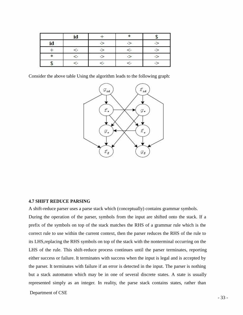
Consider the above table Using the algorithm leads to the following graph:

4.7 SHIFT REDUCE PARSING

A shift-reduce parser uses a parse stack which (conceptually) contains grammar symbols.

During the operation of the parser, symbols from the input are shifted onto the stack. If a

prefix of the symbols on top of the stack matches the RHS of a grammar rule which is the

correct rule to use within the current context, then the parser reduces the RHS of the rule to

its LHS,replacing the RHS symbols on top of the stack with the nonterminal occurring on the

LHS of the rule. This shift-reduce process continues until the parser terminates, reporting

either success or failure. It terminates with success when the input is legal and is accepted by

the parser. It terminates with failure if an error is detected in the input. The parser is nothing

but a stack automaton which may be in one of several discrete states. A state is usually

represented simply as an integer. In reality, the parse stack contains states, rather than

Department of CSE

- 33 -

grammar symbols. However, since each state corresponds to a unique grammar symbol, the

state stack can be mapped onto the grammar symbol stack mentioned earlier.

The operation of the parser is controlled by a couple of tables:

4.8 ACTION TABLE

The action table is a table with rows indexed by states and columns indexed by terminal

symbols. When the parser is in some state s and the current lookahead terminal is t, the

action taken by the parser depends on the contents of action[s][t], which can contain four

different kinds of entries:

Shift s'

Shift state s' onto the parse stack.

Reduce r

Reduce by rule r. This is explained in more detail below.

Accept

Terminate the parse with success, accepting the input.

Error

Signal a parse error

4.9 GOTO TABLE

The goto table is a table with rows indexed by states and columns indexed by nonterminal

symbols. When the parser is in state s immediately after reducing by rule N, then the next

state to enter is given by goto[s][N].

The current state of a shift-reduce parser is the state on top of the state stack. The detailed

operation of such a parser is as follows:

1. Initialize the parse stack to contain a single state s0, where s0 is the distinguished initial

state of the parser.

2. Use the state s on top of the parse stack and the current lookahead t to consult the action

table entry action[s][t]:

· If the action table entry is shift s' then push state s' onto the stack and advance the

input so that the lookahead is set to the next token.

· If the action table entry is reduce r and rule r has m symbols in its RHS, then pop

m symbols off the parse stack. Let s' be the state now revealed on top of the parse

stack and N be the LHS nonterminal for rule r. Then consult the goto table and

Department of CSE

- 34 -

push the state given by goto[s'][N] onto the stack. The lookahead token is not

changed by this step.

If the action table entry is accept, then terminate the parse with success.

If the action table entry is error, then signal an error.

3. Repeat step (2) until the parser terminates.

For example, consider the following simple grammar

0) $S: stmt <EOF>

1) stmt: ID ':=' expr

2) expr: expr '+' ID

3) expr: expr '-' ID

4) expr: ID

which describes assignment statements like a:= b + c - d. (Rule 0 is a special augmenting

production added to the grammar).

One possible set of shift-reduce parsing tables is shown below (sn denotes shift n, rn denotes

reduce n, acc denotes accept and blank entries denote error entries):

Parser Tables


4.10 SLR PARSER

An LR(0) item (or just item) of a grammar G is a production of G with a dot at some position

of the right side indicating how much of a production we have seen up to a given point.

For example, for the production E -> E + T we would have the following items:

[E -> .E + T]

[E -> E. + T]

[E -> E +. T]

[E -> E + T.]

Department of CSE

- 36 -

4.11 CONSTRUCTING THE SLR PARSING TABLE

To construct the parser table we must convert our NFA into a DFA. The states in the LR

table will be the e-closures of the states corresponding to the items SO...the process of

creating the LR state table parallels the process of constructing an equivalent DFA from a

machine with e-transitions. Been there, done that - this is essentially the subset construction

algorithm so we are in familiar territory here.

We need two operations: closure()

and goto().

closure()

If I is a set of items for a grammar G, then closure(I) is the set of items constructed from I by

the two rules: Initially every item in I is added to closure(I)

If A -> a.Bb is in closure(I), and B -> g is a production, then add the initial item [B -> .g] to I,

if it is not already there. Apply this rule until no more new items can be added to closure(I).

From our grammar above, if I is the set of one item {[E'-> .E]}, then closure(I) contains:

I0: E' -> .E

E -> .E + T

E -> .T

T -> .T * F

T -> .F

F -> .(E)

F -> .id

goto()

goto(I, X), where I is a set of items and X is a grammar symbol, is defined to be the closure

of the set of all items [A -> aX.b] such that [A -> a.Xb] is in I. The idea here is fairly intuitive:

if I is the set of items that are valid for some viable prefix g, then goto(I, X) is the set of items

that are valid for the viable prefix gX.

4.12 SETS-OF-ITEMS-CONSTRUCTION

To construct the canonical collection of sets of LR(0) items for

augmented grammar G'.

procedure items(G')

begin

Department of CSE

- 37 -

C := {closure({[S' -> .S]})};

repeat

for each set of items in C and each grammar symbol X

such that goto(I, X) is not empty and not in C do

add goto(I, X) to C;

until no more sets of items can be added to C

end;

4.13 ALGORITHM FOR CONSTRUCTING AN SLR PARSING TABLE

Input: augmented grammar G'

Output: SLR parsing table functions action and goto for G'

Method:

Construct C = {I0, I1 , ..., In} the collection of sets of LR(0) items for G'.

State i is constructed from Ii:

if [A -> a.ab] is in Ii and goto(Ii, a) = Ij, then set action[i, a] to "shift j". Here a must be a

terminal.

if [A -> a.] is in Ii, then set action[i, a] to "reduce A -> a" for all a in FOLLOW(A). Here A

may

not be S'.

if [S' -> S.] is in Ii, then set action[i, $] to "accept"

If any conflicting actions are generated by these rules, the grammar is not SLR(1) and the

algorithm fails to produce a parser. The goto transitions for state i are constructed for all

nonterminals A using the rule: If goto(Ii, A)= Ij, then goto[i, A] = j.

All entries not defined by rules 2 and 3 are made "error".

The inital state of the parser is the one constructed from the set of items containing [S' -> .S].

Let's work an example to get a feel for what is going on,

An Example

(1) E -> E * B

(2) E -> E + B

(3) E -> B

(4) B -> 0

(5) B -> 1

Department of CSE

- 38 -

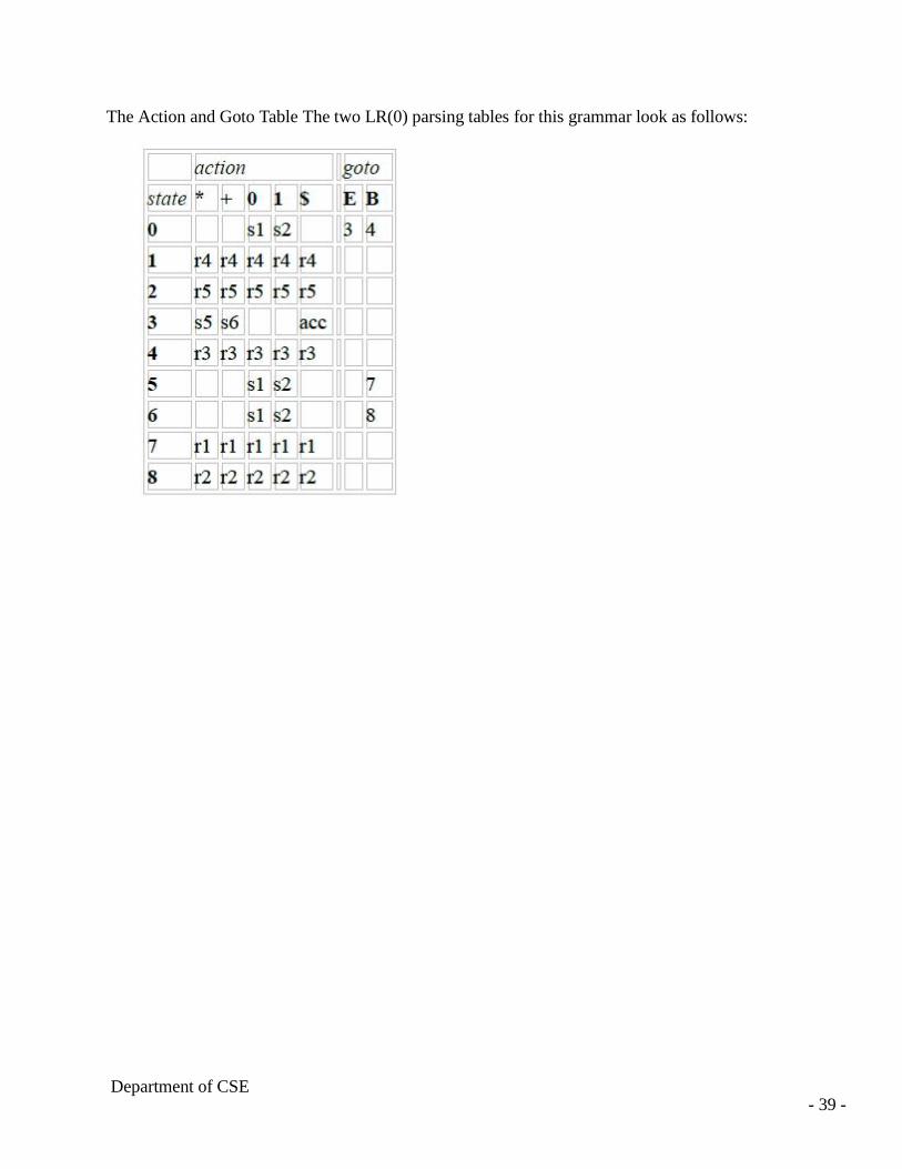
The Action and Goto Table The two LR(0) parsing tables for this grammar look as follows:

Department of CSE

- 39 -

UNIT -5

5.1 CANONICAL LR PARSING

By splitting states when necessary, we can arrange to have each state of an LR parser

indicate exactly which input symbols can follow a handle a for which there is a possible

reduction to A. As the text points out, sometimes the FOLLOW sets give too much

informationand doesn't (can't) discriminate between different reductions.

The general form of an LR(k) item becomes [A -> a.b, s] where A -> ab is a production and s

is a string of terminals. The first part (A -> a.b) is called the core and the second part is the

lookahead. In LR(1) |s| is 1, so s is a single terminal.

A -> ab is the usual righthand side with a marker; any a in s is an incoming token in which

we are interested. Completed items used to be reduced for every incoming token in

FOLLOW(A), but now we will reduce only if the next input token is in the lookahead set s..if

we get two productions A -> a and B -> a, we can tell them apart when a is a handle on the

stack if the corresponding completed items have different lookahead parts. Furthermore, note

that the lookahead has no effect for an item of the form [A -> a.b, a] if b is not e. Recall that

our problem occurs for completed items, so what we have done now is to say that an item of

the form [A -> a., a] calls for a reduction by A -> a only if the next input symbol is a. More

formally, an LR(1) item [A -> a.b, a] is valid for a viable prefix g if there is a derivation

S =>* s abw, where g = sa, and either a is the first symbol of w, or w is e and a is $.

5.2 ALGORITHM FOR CONSTRUCTION OF THE SETS OF LR(1) ITEMS

Input: grammar G'

Output: sets of LR(1) items that are the set of items valid for one or more viable prefixes of

G'

Method:

closure(I)

begin

repeat

for each item [A -> a.Bb, a] in I,

each production B -> g in G',

and each terminal b in FIRST(ba)

Department of CSE

- 40 -

such that [B -> .g, b] is not in I do

add [B -> .g, b] to I;

until no more items can be added to I;

end;

5.3 goto(I, X)

begin

let J be the set of items [A -> aX.b, a] such that

[A -> a.Xb, a] is in I

return closure(J);

end;

procedure items(G')

begin

C := {closure({S' -> .S, $})};

repeat

for each set of items I in C and each grammar symbol X such

that goto(I, X) is not empty and not in C do

add goto(I, X) to C

until no more sets of items can be added to C;

end;

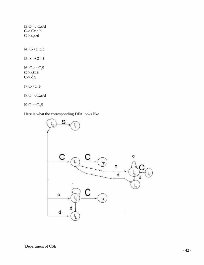
An example,

Consider the following grammer,

S’->S

S->CC

C->cC

C->d

Sets of LR(1) items

I0: S’->.S,$

S->.CC,$

C->.Cc,c/d

C->.d,c/d

I1:S’->S.,$

I2:S->C.C,$

C->.Cc,$

C->.d,$ Department of CSE

- 41 -

I3:C->c.C,c/d

C->.Cc,c/d

C->.d,c/d

I4: C->d.,c/d

I5: S->CC.,$

I6: C->c.C,$

C->.cC,$

C->.d,$

I7:C->d.,$

I8:C->cC.,c/d

I9:C->cC.,$

Here is what the corresponding DFA looks like


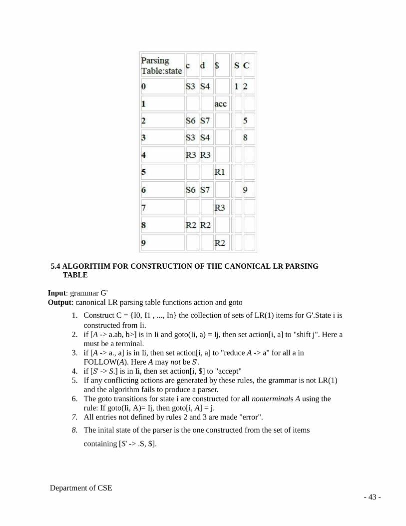
5.4 ALGORITHM FOR CONSTRUCTION OF THE CANONICAL LR PARSING

TABLE

Input: grammar G'

Output: canonical LR parsing table functions action and goto

1. Construct C = {I0, I1 , ..., In} the collection of sets of LR(1) items for G'.State i is

constructed from Ii. 2. if [A -> a.ab, b>] is in Ii and goto(Ii, a) = Ij, then set action[i, a] to "shift j". Here a

must be a terminal.

3. if [A -> a., a] is in Ii, then set action[i, a] to "reduce A -> a" for all a in

FOLLOW(A). Here A may not be S'.

4. if [S' -> S.] is in Ii, then set action[i, $] to "accept"

5. If any conflicting actions are generated by these rules, the grammar is not LR(1)

and the algorithm fails to produce a parser.

6. The goto transitions for state i are constructed for all nonterminals A using the

rule: If goto(Ii, A)= Ij, then goto[i, A] = j. 7. All entries not defined by rules 2 and 3 are made "error".

8. The inital state of the parser is the one constructed from the set of items

containing [S' -> .S, $].

Department of CSE

- 43 -

5.5.LALR PARSER:

We begin with two observations. First, some of the states generated for LR(1) parsing have

the same set of core (or first) components and differ only in their second component, the

lookahead symbol. Our intuition is that we should be able to merge these states and reduce

the number of states we have, getting close to the number of states that would be generated

for LR(0) parsing. This observation suggests a hybrid approach: We can construct the

canonical LR(1) sets of items and then look for sets of items having the same core. We merge

these sets with common cores into one set of items. The merging of states with common

cores can never produce a shift/reduce conflict that was not present in one of the original

states because shift actions depend only on the core, not the lookahead. But it is possible for

the merger to produce a reduce/reduce conflict.

Our second observation is that we are really only interested in the lookahead symbol in

places where there is a problem. So our next thought is to take the LR(0) set of items and add

lookaheads only where they are needed. This leads to a more efficient, but much more

complicated method.

5.6 ALGORITHM FOR EASY CONSTRUCTION OF AN LALR TABLE

Input: G'

Output: LALR parsing table functions with action and goto for G'.

Method:

1. Construct C = {I0, I1 , ..., In} the collection of sets of LR(1) items for G'.

2. For each core present among the set of LR(1) items, find all sets having that core

and replace these sets by the union.

3. Let C' = {J0, J1 , ..., Jm} be the resulting sets of LR(1) items. The parsing actions

for state i are constructed from Ji in the same manner as in the construction of the

canonical LR parsing table.

4. If there is a conflict, the grammar is not LALR(1) and the algorithm fails.

5. The goto table is constructed as follows: If J is the union of one or more sets of

LR(1) items, that is, J = I0U I1 U ... U Ik, then the cores of goto(I0, X), goto(I1,

X), ..., goto(Ik, X) are the same, since I0, I1 , ..., Ik all have the same core. Let K

be the union of all sets of items having the same core asgoto(I1, X).


5.7HANDLING ERRORS

6. Then goto(J, X) = K.

Consider the above example,

I3 & I6 can be replaced by their union

I36:C->c.C,c/d/$

C->.Cc,C/D/$

C->.d,c/d/$

I47:C->d.,c/d/$

I89:C->Cc.,c/d/$

Parsing Table

The LALR parser may continue to do reductions after the LR parser would have spotted an

error, but the LALR parser will never do a shift after the point the LR parser would have

discovered the error and will eventually find the error.

5.8 DANGLING ELSE

The dangling else is a problem in computer programming in which an optional else clause in

an If–then(–else) statement results in nested conditionals being ambiguous. Formally,

the context-free grammar of the language is ambiguous, meaning there is more than one

correct parse tree.


state c d $ S C

0 S36 S47 1 2

1 Accept

2 S36 S47 5

36 S36 S47 89

47 R3 R3

5 R1

89 R2 R2 R2

In many programming languages one may write conditionally executed code in two forms:

the if-then form, and the if-then-else form – the else clause is optional:

Consider the grammar:

S ::= E $

E ::= E + E

|E*E

|(E)

| id

| num

and four of its LALR(1) states:

I0: S ::= . E $ ?

E ::= . E + E +*$ I1: S ::= E . $ ? I2: E ::= E * . E +*$

E ::= . E * E +*$ E ::= E . + E +*$ E ::= . E + E +*$

E ::= . ( E ) +*$ E ::= E . * E +*$ E ::= . E * E +*$

E ::= . id +*$ E ::= . ( E ) +*$

E ::= . num +*$ I3: E ::= E * E . +*$ E ::= . id +*$

E ::= E . + E +*$ E ::= . num +*$


E ::= E . * E +*$

Here we have a shift-reduce error. Consider the first two items in I3. If we have a*b+c and

we parsed a*b, do we reduce using E ::= E * E or do we shift more symbols? In the former

case we get a parse tree (a*b)+c; in the latter case we get a*(b+c). To resolve this conflict, we

can specify that * has higher precedence than +. The precedence of a grammar production is

equal to the precedence of the rightmost token at the rhs of the production. For example, the

precedence of the production E ::= E * E is equal to the precedence of the operator *, the

precedence of the production E ::= ( E ) is equal to the precedence of the token ), and the

precedence of the production E ::= if E then E else E is equal to the precedence of the token

else. The idea is that if the look ahead has higher precedence than the production currently

used, we shift. For example, if we are parsing E + E using the production rule E ::= E + E

and the look ahead is *, we shift *. If the look ahead has the same precedence as that of the

current production and is left associative, we reduce, otherwise we shift. The above grammar

is valid if we define the precedence and associativity of all the operators. Thus, it is very

important when you write a parser using CUP or any other LALR(1) parser generator to

specify associativities and precedence’s for most tokens (especially for those used as

operators). Note: you can explicitly define the precedence of a rule in CUP using the %prec

directive:

E ::= MINUS E %prec UMINUS

where UMINUS is a pseudo-token that has higher precedence than TIMES, MINUS etc, so

that -1*2 is equal to (-1)*2, not to -(1*2).

Another thing we can do when specifying an LALR(1) grammar for a parser generator is

error recovery. All the entries in the ACTION and GOTO tables that have no content

correspond to syntax errors. The simplest thing to do in case of error is to report it and stop

the parsing. But we would like to continue parsing finding more errors. This is called error

recovery. Consider the grammar:

S ::= L = E ;

| { SL } ;

| error ;

SL ::= S ;

| SL S ;


The special token error indicates to the parser what to do in case of invalid syntax for S (an

invalid statement). In this case, it reads all the tokens from the input stream until it finds the

first semicolon. The way the parser handles this is to first push an error state in the stack. In

case of an error, the parser pops out elements from the stack until it finds an error state where

it can proceed. Then it discards tokens from the input until a restart is possible. Inserting

error handling productions in the proper places in a grammar to do good error recovery is

considered very hard.

5.9LR ERROR RECOVERY

An LR parser will detect an error when it consults the parsing action table and find a blank or

error entry. Errors are never detected by consulting the goto table. An LR parser will detect

an error as soon as there is no valid continuation for the portion of the input thus far scanned.

A canonical LR parser will not make even a single reduction before announcing the error.

SLR and LALR parsers may make several reductions before detecting an error, but they will

never shift an erroneous input symbol onto the stack.

5.10 PANIC-MODE ERROR RECOVERY

We can implement panic-mode error recovery by scanning down the stack until a state s with

a goto on a particular nonterminal A is found. Zero or more input symbols are then discarded

until a symbol a is found that can legitimately follow A. The parser then stacks the state

GOTO(s, A) and resumes normal parsing. The situation might exist where there is more than

one choice for the nonterminal A. Normally these would be nonterminals representing major

program pieces, e.g. an expression, a statement, or a block. For example, if A is the

nonterminal stmt, a might be semicolon or }, which marks the end of a statement sequence.

This method of error recovery attempts to eliminate the phrase containing the syntactic error.

The parser determines that a string derivable from A contains an error. Part of that string has

already been processed, and the result of this processing is a sequence of states on top of the

stack. The remainder of the string is still in the input, and the parser attempts to skip over the

remainder of this string by looking for a symbol on the input that can legitimately follow A.

By removing states from the stack, skipping over the input, and pushing GOTO(s, A) on the

stack, the parser pretends that if has found an instance of A and resumes normal parsing.

Department of CSE

- 48 -

5.11 PHRASE-LEVEL RECOVERY

Phrase-level recovery is implemented by examining each error entry in the LR action table

and deciding on the basis of language usage the most likely programmer error that would

give rise to that error. An appropriate recovery procedure can then be constructed;

presumably the top of the stack and/or first input symbol would be modified in a way deemed

appropriate for each error entry. In designing specific error-handling routines for an LR

parser, we can fill in each blank entry in the action field with a pointer to an error routine that

will take the appropriate action selected by the compiler designer.

The actions may include insertion or deletion of symbols from the stack or the input or both,

or alteration and transposition of input symbols. We must make our choices so that the LR

parser will not get into an infinite loop. A safe strategy will assure that at least one input

symbol will be removed or shifted eventually, or that the stack will eventually shrink if the

end of the input has been reached. Popping a stack state that covers a non terminal should be

avoided, because this modification eliminates from the stack a construct that has already been

successfully parsed.

Department of CSE

- 49 -

UNIT 6

SEMANTIC ANALYSIS

6.1 SEMANTIC ANALYSIS

Semantic Analysis computes additional information related to the meaning of the

program once the syntactic structure is known.

In typed languages as C, semantic analysis involves adding information to the symbol

table and performing type checking.

The information to be computed is beyond the capabilities of standard parsing

techniques, therefore it is not regarded as syntax.

As for Lexical and Syntax analysis, also for Semantic Analysis we need both a

Representation Formalism and an Implementation Mechanism.

As representation formalism this lecture illustrates what are called Syntax Directed

Translations.

6.2 SYNTAX DIRECTED TRANSLATION

The Principle of Syntax Directed Translation states that the meaning of an input

sentence is related to its syntactic structure, i.e., to its Parse-Tree.

By Syntax Directed Translations we indicate those formalisms for specifying

translations for programming language constructs guided by context-free grammars.

o We associate Attributes to the grammar symbols representing the language

constructs.

o Values for attributes are computed by Semantic Rules associated with

grammar productions.

Evaluation of Semantic Rules may:

o Generate Code;

o Insert information into the Symbol Table;

o Perform Semantic Check;

o Issue error messages;

o etc.

Department of CSE

- 50 -

There are two notations for attaching semantic rules:

1. Syntax Directed Definitions. High-level specification hiding many implementation

details (also called Attribute Grammars).

2. Translation Schemes. More implementation oriented: Indicate the order in which

semantic rules are to be evaluated.

Syntax Directed Definitions

• Syntax Directed Definitions are a generalization of context-free grammars in which:

1. Grammar symbols have an associated set of Attributes;

2. Productions are associated with Semantic Rules for computing the values of attributes.

Such formalism generates Annotated Parse-Trees where each node of the tree is a

record with a field for each attribute (e.g.,X.a indicates the attribute a of the grammar

symbol X).

The value of an attribute of a grammar symbol at a given parse-tree node is defined by

a semantic rule associated with the production used at that node.

We distinguish between two kinds of attributes:

1. Synthesized Attributes. They are computed from the values of the attributes of the

children nodes.

2. Inherited Attributes. They are computed from the values of the attributes of both the

siblings and the parent nodes

Syntax Directed Definitions: An Example

• Example. Let us consider the Grammar for arithmetic expressions. The

Syntax Directed Definition associates to each non terminal a synthesized

attribute called val.

Department of CSE

- 51 -

6.3 S-ATTRIBUTED DEFINITIONS

Definition. An S-Attributed Definition is a Syntax Directed Definition that uses

only synthesized attributes.

• Evaluation Order. Semantic rules in a S-Attributed Definition can be

evaluated by a bottom-up, or PostOrder, traversal of the parse-tree.

• Example. The above arithmetic grammar is an example of an S-Attributed

Definition. The annotated parse-tree for the input 3*5+4n is:

Department of CSE

- 52 -

6.4 L-attributed definition

Definition: A SDD its L-attributed if each inherited attribute of Xi in the RHS of A ! X1 :

:Xn depends only on

1. attributes of X1;X2; : : : ;Xi�1 (symbols to the left of Xi in the RHS)

2. inherited attributes of A.

Restrictions for translation schemes:

1. Inherited attribute of Xi must be computed by an action before Xi.

2. An action must not refer to synthesized attribute of any symbol to the right of that action.

3. Synthesized attribute for A can only be computed after all attributes it references have

been completed (usually at end of RHS).

6.5 SYMBOL TABLES

A symbol table is a major data structure used in a compiler. Associates attributes with

identifiers used in a program. For instance, a type attribute is usually associated with each

identifier. A symbol table is a necessary component Definition (declaration) of identifiers

appears once in a program .Use of identifiers may appear in many places of the program text

Identifiers and attributes are entered by the analysis phases. When processing a definition

(declaration) of an identifier. In simple languages with only global variables and implicit

declarations. The scanner can enter an identifier into a symbol table if it is not already there

In block-structured languages with scopes and explicit declarations:

The parser and/or semantic analyzer enter identifiers and corresponding attributes

Symbol table information is used by the analysis and synthesis phases

To verify that used identifiers have been defined (declared)

To verify that expressions and assignments are semantically correct – type checking

To generate intermediate or target code

Symbol Table Interface

The basic operations defined on a symbol table include:

allocate – to allocate a new empty symbol table

free – to remove all entries and free the storage of a symbol table

insert – to insert a name in a symbol table and return a pointer to its entry

Department of CSE

- 53 -

lookup – to search for a name and return a pointer to its entry

set_attribute – to associate an attribute with a given entry

get_attribute – to get an attribute associated with a given entry

Other operations can be added depending on requirement For example, a delete operation

removes a name previously inserted Some identifiers become invisible (out of scope) after

exiting a block

This interface provides an abstract view of a symbol table

Supports the simultaneous existence of multiple tables

Implementation can vary without modifying the interface

Basic Implementation Techniques

First consideration is how to insert and lookup names

Variety of implementation techniques

Unordered List

Simplest to implement

Implemented as an array or a linked list

Linked list can grow dynamically – alleviates problem of a fixed size array

Insertion is fast O(1), but lookup is slow for large tables – O(n) on average

Ordered List

If an array is sorted, it can be searched using binary search – O(log2 n)

Insertion into a sorted array is expensive – O(n) on average

Useful when set of names is known in advance – table of reserved words

Binary Search Tree

Can grow dynamically

Insertion and lookup are O(log2 n) on average

6.6 HASH TABLES AND HASH FUNCTIONS

A hash table is an array with index range: 0 to TableSize – 1

Most commonly used data structure to implement symbol tables

Insertion and lookup can be made very fast – O(1)

A hash function maps an identifier name into a table index

Department of CSE

- 54 -

A hash function, h(name), should depend solely on name

h(name) should be computed quickly

h should be uniform and randomizing in distributing names

All table indices should be mapped with equal probability.

Similar names should not cluster to the same table index

6.7 HASH FUNCTIONS

_ Hash functions can be defined in many ways . . .

_ A string can be treated as a sequence of integer words

_ Several characters are fit into an integer word

_ Strings longer than one word are folded using exclusive-or or addition

_ Hash value is obtained by taking integer word modulo TableSize

_ We can also compute a hash value character by character:

_ h(name) = (c0 + c1 + … + cn–1) mod TableSize, where n is name length

_ h(name) = (c0 * c1 * … * cn–1) mod TableSize

_ h(name) = (cn–1 + ___ cn–2 + … + ___ c1 + __c0))) mod TableSize

_ h(name) = (c0 * cn–1 * n) mod TableSize

6.8 RUNTIME ENVIRONMENT

Runtime organization of different storage locations

Representation of scopes and extents during program execution.

Components of executing program reside in blocks of memory (supplied by OS).

Three kinds of entities that need to be managed at runtime:

o Generated code for various procedures and programs.

forms text or code segment of your program: size known at compile time.

o Data objects:

Global variables/constants: size known at compile time

Variables declared within procedures/blocks: size known

Variables created dynamically: size unknown.

o Stack to keep track of procedure activations.

Subdivide memory conceptually into code and data areas:

Department of CSE

- 55 -

Code: Program

instructions

Stack: Manage activation of procedures at runtime.

Heap: holds variables created dynamically

6.9 STORAGE ORGANIZATION

1Fixed-size objects can be placed in predefined locations.

2. Run-time stack and heap

The STACK is used to store:

o Procedure activations.

o The status of the machine just before calling a procedure, so that the status can be

restored when the called procedure returns.

o The HEAP stores data allocated under program control (e.g. by malloc() in C).

Department of CSE

- 56 -

Activation records

Any information needed for a single activation of a procedure is stored in the

ACTIVATION RECORD (sometimes called the STACK FRAME). Today, we’ll assume the

stack grows DOWNWARD, as on, e.g., the Intel architecture. The activation record gets

pushed for each procedure call and popped for each procedure return.

6.9 STATIC ALLOCATION

Statically allocated names are bound to storage at compile time. Storage bindings of

statically allocated names never change, so even if a name is local to a procedure, its name is

always bound to the same storage. The compiler uses the type of a name (retrieved from the

symbol table) to determine storage size required. The required number of bytes (possibly

aligned) is set aside for the name.The address of the storage is fixed at compile time.

Limitations:

− The size required must be known at compile time.

− Recursive procedures cannot be implemented as all locals are statically

allocated.

− No data structure can be created dynamically as all data is static.

Stack-dynamic allocation

Storage is organized as a stack.

Activation records are pushed and popped.

Locals and parameters are contained in the activation records for the call.

This means locals are bound to fresh storage on every call.

If we have a stack growing downwards, we just need a stack_top pointer.

To allocate a new activation record, we just increase stack_top.

To deallocate an existing activation record, we just decrease stack_top.

Address generation in stack allocation

The position of the activation record on the stack cannot be determined statically.

Therefore the compiler must generate addresses RELATIVE to the activation record. If we

have a downward-growing stack and a stack_top pointer, we generate addresses of the form

stack_top + offset

Department of CSE

- 57 -

6.10 HEAP ALLOCATION

Some languages do not have tree-structured allocations. In these cases, activations

have to be allocated on the heap. This allows strange situations, like callee activations that

live longer than their callers’ activations. This is not common Heap is used for allocating

space for objects created at run timeFor example: nodes of dynamic data structures such as

linked lists and trees

�Dynamic memory allocation and deallocation based on the requirements of the

programmalloc() and free() in C programs

new()and delete()in C++ programs

new()and garbage collection in Java programs

�Allocation and deallocation may be completely manual (C/C++), semi-automatic(Java), or

fully automatic (Lisp)

6.11 PARAMETERS PASSING

A language has first-class functionsif functions can bedeclared within any scope

passed as arguments to other functions returned as results of functions.�In a language with

first-class functions and static scope, a function value is generally represented by a closure. a

pair consisting of a pointer to function code a pointer to an activation record.�Passing

functions as arguments is very useful in structuring of systems using upcalls

An example:

main()

{ int x = 4;

int f (int y) {

return x*y;

}

int g (int →int h){

int x = 7;

return h(3) + x;

}

Department of CSE

- 58 -

g(f);//returns 12

}

Passing Functions as Parameters – Implementation with Static Scope

Department of CSE

- 59 -

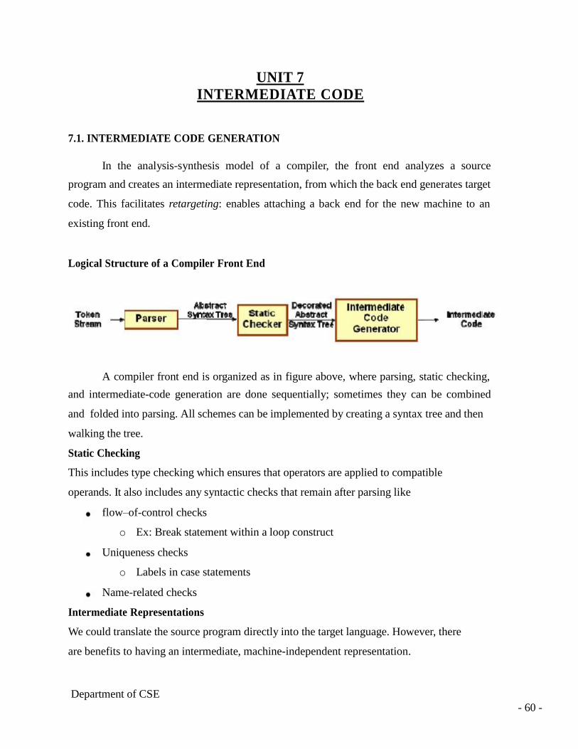
UNIT 7

INTERMEDIATE CODE

7.1. INTERMEDIATE CODE GENERATION

In the analysis-synthesis model of a compiler, the front end analyzes a source

program and creates an intermediate representation, from which the back end generates target

code. This facilitates retargeting: enables attaching a back end for the new machine to an

existing front end.

Logical Structure of a Compiler Front End

A compiler front end is organized as in figure above, where parsing, static checking,

and intermediate-code generation are done sequentially; sometimes they can be combined

and folded into parsing. All schemes can be implemented by creating a syntax tree and then

walking the tree.

Static Checking

This includes type checking which ensures that operators are applied to compatible

operands. It also includes any syntactic checks that remain after parsing like

flow–of-control checks

o Ex: Break statement within a loop construct

Uniqueness checks

o Labels in case statements

Name-related checks

Intermediate Representations

We could translate the source program directly into the target language. However, there

are benefits to having an intermediate, machine-independent representation.

Department of CSE

- 60 -

A clear distinction between the machine-independent and machine-dependent parts of

the compiler

Retargeting is facilitated the implementation of language processors for new

machines will require replacing only the back-end.

We could apply machine independent code optimization techniques

Intermediate representations span the gap between the source and target languages.

• High Level Representations

closer to the source language

easy to generate from an input program

code optimizations may not be straightforward

• Low Level Representations

closer to the target machine

Suitable for register allocation and instruction selection

easier for optimizations, final code generation

There are several options for intermediate code. They can be either

• Specific to the language being implemented

P-code for Pascal

Byte code for Java

7.2 LANGUAGE INDEPENDENT 3-ADDRESS CODE

IR can be either an actual language or a group of internal data structures that are shared by

the phases of the compiler. C used as intermediate language as it is flexible, compiles into

efficient machine code and its compilers are widely available.In all cases, the intermediate

code is a linearization of the syntax tree produced during syntax and semantic analysis. It is

formed by breaking down the tree structure into sequential instructions, each of which is

equivalent to a single, or small number of machine instructions. Machine code can then be

generated (access might be required to symbol tables etc). TAC can range from high- to low-

level, depending on the choice of operators. In general, it is a statement containing at most 3

addresses or operands.

The general form is x := y op z, where “op” is an operator, x is the result, and y and z are

operands. x, y, z are variables, constants, or “temporaries”. A three-address instruction

Department of CSE

- 61 -

consists of at most 3 addresses for each statement.

It is a linear zed representation of a binary syntax tree. Explicit names correspond to interior

nodes of the graph. E.g. for a looping statement , syntax tree represents components of the

statement, whereas three-address code contains labels and jump instructions to represent the

flow-of-control as in machine language. A TAC instruction has at most one operator on the

RHS of an instruction; no built-up arithmetic expressions are permitted.

e.g. x + y * z can be translated as

t1 = y * z

t2 = x + t1

Where t1 & t2 are compiler–generated temporary names.

5Since it unravels multi-operator arithmetic expressions and nested control-flow statements,

it is useful for target code generation and optimization.

Addresses and Instructions

• TAC consists of a sequence of instructions, each instruction may have up to three

addresses, prototypically t1 = t2 op t3

• Addresses may be one of:

o A name. Each name is a symbol table index. For convenience, we writethe names

as the identifier.

o A constant.

o A compiler-generated temporary. Each time a temporary address is needed, the

compiler generates another name from the stream t1, t2, t3, etc.

• Temporary names allow for code optimization to easily move Instructions

• At target-code generation time, these names will be allocated to registers or to memory.

• TAC Instructions

o Symbolic labels will be used by instructions that alter the flow of control.

The instruction addresses of labels will be filled in later.

L: t1 = t2 op t3

o Assignment instructions: x = y op z

• Includes binary arithmetic and logical operations

o Unary assignments: x = op y

Department of CSE

- 62 -

• Includes unary arithmetic op (-) and logical op (!) and type

conversion

o Copy instructions: x = y

o Unconditional jump: goto L

• L is a symbolic label of an instruction

o Conditional jumps:

if x goto L If x is true, execute instruction L next

ifFalse x goto L If x is false, execute instruction L next

o Conditional jumps:

if x relop y goto L

– Procedure calls. For a procedure call p(x1, …, xn)

param x1

…

param xn

call p, n

– Function calls : y= p(x1, …, xn) y = call p,n , return y

– Indexed copy instructions: x = y[i] and x[i] = y

Left: sets x to the value in the location i memory units beyond y

Right: sets the contents of the location i memory units beyond x to y

– Address and pointer instructions:

• x = &y sets the value of x to be the location (address) of y.

• x = *y, presumably y is a pointer or temporary whose value is a

location. The value of x is set to the contents of that location.

• *x = y sets the value of the object pointed to by x to the value of y.

Example: Given the statement do i = i+1; while (a[i] < v ); , the TAC can be written as

below in two ways, using either symbolic labels or position number of instructions for

labels.

Department of CSE

- 63 -

Types of three address code

There are different types of statements in source program to which three address code has to

be generated. Along with operands and operators, three address code also use labels to

provide flow of control for statements like if-then-else, for and while. The different types of

three address code statements are:

Assignment statement

a = b op c

In the above case b and c are operands, while op is binary or logical operator. The result of

applying op on b and c is stored in a.

Unary operation

a = op b This is used for unary minus or logical negation.

Example: a = b * (- c) + d

Three address code for the above example will be

t1 = -c

t2 = t1 * b

t3 = t2 + d

a = t3

Copy Statement

a=b

The value of b is stored in variable a.

Unconditional jump

goto L

Creates label L and generates three-address code ‘goto L’

v. Creates label L, generate code for expression exp, If the exp returns value true then go to

the statement labelled L. exp returns a value false go to the statement immediately following

the if statement.

Function call

For a function fun with n arguments a1,a2,a3….an ie.,

fun(a1, a2, a3,…an),

Department of CSE

- 64 -

the three address code will be

Param a1

Param a2

…

Param an

Call fun, n

Where param defines the arguments to function.

Array indexing

In order to access the elements of array either single dimension or

multidimension, three address code requires base address and offset value. Base address

consists of the address of first element in an array. Other elements of the array can be

accessed using the base address and offset value.

Example: x = y[i]

Memory location m = Base address of y + Displacement i

x = contents of memory location m

similarly x[i] = y

Memory location m = Base address of x + Displacement i

The value of y is stored in memory location m

Pointer assignment

x = &y x stores the address of memory location y

x = *y y is a pointer whose r-value is location

*x = y sets r-value of the object pointed by x to the r-value of y

Intermediate representation should have an operator set which is rich to implement most of

the

operations of source language. It should also help in mapping to restricted instruction set of

target machine.

Data Structure

Three address code is represented as record structure with fields for operator and operands.

These

Department of CSE

- 65 -

records can be stored as array or linked list. Most common implementations of three address

code are-

Quadruples, Triples and Indirect triples.

7.3 QUADRUPLES-

Quadruples consists of four fields in the record structure. One field to store operator op, two

fields to store operands or arguments arg1and arg2 and one field to store result res. res = arg1

op arg2

Example: a = b + c

b is represented as arg1, c is represented as arg2, + as op and a as res.

Unary operators like ‘-‘do not use agr2. Operators like param do not use agr2 nor result. For

conditional and unconditional statements res is label. Arg1, arg2 and res are pointers to

symbol table or literal table for the names.

Example: a = -b * d + c + (-b) * d

Three address code for the above statement is as follows

t1 = - b

t2 = t1 * d

t3 = t2 + c

t4 = - b

t5 = t4 * d

t6 = t3 + t5

a = t6

Quadruples for the above example is as follows

Department of CSE

- 66 -

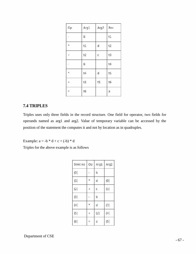
7.4 TRIPLES

Triples uses only three fields in the record structure. One field for operator, two fields for

operands named as arg1 and arg2. Value of temporary variable can be accessed by the

position of the statement the computes it and not by location as in quadruples.

Example: a = -b * d + c + (-b) * d

Triples for the above example is as follows


Arg1 and arg2 may be pointers to symbol table for program variables or literal table for

constant or pointers into triple structure for intermediate results.

Example: Triples for statement x[i] = y which generates two records is as follows

Triples for statement x = y[i] which generates two records is as follows

Triples are alternative ways for representing syntax tree or Directed acyclic graph for

program defined names.

Indirect Triples

Indirect triples are used to achieve indirection in listing of pointers. That is, it uses pointers to

triples than listing of triples themselves.

Example: a = -b * d + c + (-b) * d


Conditional operator and operands. Representations include quadruples, triples and indirect

triples.

7.5 SYNTAX TREES

Syntax trees are high level IR. They depict the natural hierarchical structure of the source

program. Nodes represent constructs in source program and the children of a node represent

meaningful components of the construct. Syntax trees are suited for static type checking.

Variants of Syntax Trees: DAG

A directed acyclic graph (DAG) for an expression identifies the common sub expressions

(sub expressions that occur more than once) of the expression. DAG's can be constructed

by using the same techniques that construct syntax trees.

A DAG has leaves corresponding to atomic operands and interior nodes corresponding to

operators. A node N in a DAG has more than one parent if N represents a common sub

expression, so a DAG represents expressions concisely. It gives clues to compiler about

the generating efficient code to evaluate expressions.

Example 1: Given the grammar below, for the input string id + id * id , the parse tree,

Department of CSE

- 69 -

syntax tree and the DAG are as shown.

Example : DAG for the expression a + a * (b - c) + ( b - c ) * d is shown below.

Department of CSE

- 70 -

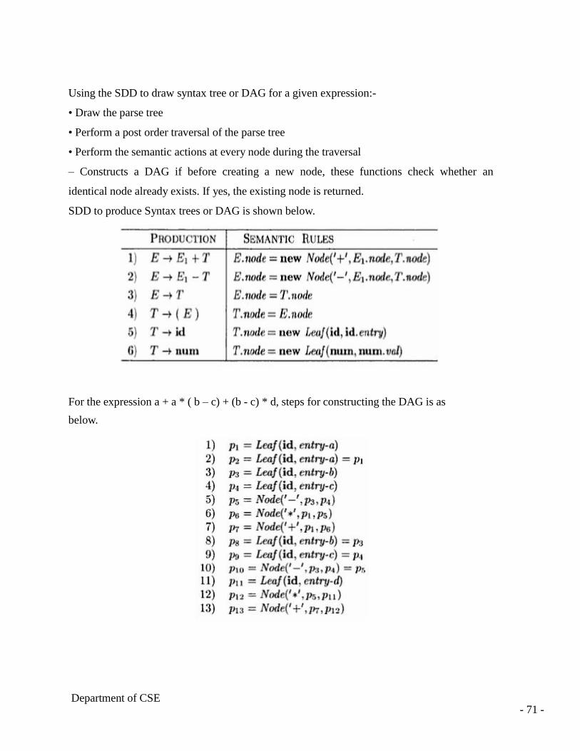
Using the SDD to draw syntax tree or DAG for a given expression:-

• Draw the parse tree

• Perform a post order traversal of the parse tree

• Perform the semantic actions at every node during the traversal

– Constructs a DAG if before creating a new node, these functions check whether an

identical node already exists. If yes, the existing node is returned.

SDD to produce Syntax trees or DAG is shown below.

For the expression a + a * ( b – c) + (b - c) * d, steps for constructing the DAG is as

below.

Department of CSE

- 71 -

7.6 BASIC BLOCKS AND FLOW GRAPHS

A graph representation of three-address statements, called a flow graph, is useful for

understanding code-generation algorithms, even if the graph is not explicitly constructed by a

code-generation algorithm. Nodes in the flow graph represent computations, and the edges

represent the flow of control. Flow graph of a program can be used as a vehicle to collect

information about the intermediate program. Some register-assignment algorithms use flow

graphs to find the inner loops where a program is expected to spend most of its time.

BASIC BLOCKS

A basic block is a sequence of consecutive statements in which flow of control

enters at the beginning and leaves at the end without halt or possibility of branching except at

the end. The following sequence of three-address statements forms a basic block:

t1 := a*a

t2 := a*b

t3 := 2*t2

t4 := t1+t3

t5 := b*b

t6 := t4+t5

A three-address statement x := y+z is said to define x and to use y or z. A name in a basic

block is said to live at a given point if its value is used after that point in the program,

perhaps in another basic block.

The following algorithm can be used to partition a sequence of three-address statements into

basic blocks.

Algorithm 1: Partition into basic blocks.

Input: A sequence of three-address statements.

Output: A list of basic blocks with each three-address statement in exactly one block.

Method:

1. We first determine the set of leaders, the first statements of basic blocks.

The rules we use are the following:

I) The first statement is a leader.

II) Any statement that is the target of a conditional or unconditional goto is a leader.

Department of CSE

- 72 -

III) Any statement that immediately follows a goto or conditional goto statement is a

leader.

2. For each leader, its basic block consists of the leader and all statements up to but not

including the next leader or the end of the program.

Example 3: Consider the fragment of source code shown in fig. 7; it computes the dot

product of two vectors a and b of length 20. A list of three-address statements performing

this computation on our target machine is shown in fig. 8.

begin

prod := 0;

i := 1;

do begin

prod := prod + a[i] * b[i];

i := i+1;

end

while i<= 20

end

Let us apply Algorithm 1 to the three-address code in fig 8 to determine its basic

blocks. statement (1) is a leader by rule (I) and statement (3) is a leader by rule (II), since the

last statement can jump to it. By rule (III) the statement following (12) is a leader. Therefore,

statements (1) and (2) form a basic block. The remainder of the program beginning with

statement (3) forms a second basic block.

(1) prod := 0

(2) i := 1

(3) t1 := 4*i

(4) t2 := a [ t1 ]

(5) t3 := 4*i

(6) t4 :=b [ t3 ]

(7) t5 := t2*t4

(8) t6 := prod +t5

(9) prod := t6

(10) t7 := i+1

Department of CSE

- 73 -

(11) i := t7

(12) if i<=20 goto (3)

7.7 TRANSFORMATIONS ON BASIC BLOCKS

A basic block computes a set of expressions. These expressions are the values of the names

live on exit from block. Two basic blocks are said to be equivalent if they compute the same

set of expressions. A number of transformations can be applied to a basic block without

changing the set of expressions computed by the block. Many of these transformations are

useful for improving the quality of code that will be ultimately generated from a basic block.

There are two important classes of local transformations that can be applied to basic blocks;

these are the structure-preserving transformations and the algebraic transformations.

7.8 STRUCTURE-PRESERVING TRANSFORMATIONS

The primary structure-preserving transformations on basic blocks are:

1. Common sub-expression elimination

2. Dead-code elimination

3. Renaming of temporary variables

4. Interchange of two independent adjacent statements

We assume basic blocks have no arrays, pointers, or procedure calls.

1. Common sub-expression elimination

Consider the basic block

a:= b+c

b:= a-d

c:= b+c

d:= a-d

The second and fourth statements compute the same expression, namely b+c-d, and hence

this basic block may be transformed into the equivalent block

a:= b+c

b:= a-d

c:= b+c d:= b

Although the 1st and 3rd statements in both cases appear to have the same expression

Department of CSE

- 74 -

on the right, the second statement redefines b. Therefore, the value of b in the 3rd

statement is different from the value of b in the 1st, and the 1st and 3rd statements do

not compute the same expression.

2. Dead-code elimination

Suppose x is dead, that is, never subsequently used, at the point where the statement

x:= y+z appears in a basic block. Then this statement may be safely removed without

changing the value of the basic block.

3. Renaming temporary variables

Suppose we have a statement t:= b+c, where t is a temporary. If we change this statement to

u:= b+c, where u is a new temporary variable, and change all uses of this instance of t to u,

then the value of the basic block is not changed.

4.Interchange of statements

Suppose we have a block with the two adjacent statements

t1:= b+c

t2:= x+y

Then we can interchange the two statements without affecting the value of the block if and

only if neither x nor y is t1 and neither b nor c is t2. A normal-form basic block permits all

statement interchanges that are possible.

7.9 DAG REPRESENTATION OF BASIC BLOCKS

The goal is to obtain a visual picture of how information flows through the block. The leaves

will show the values entering the block and as we proceed up the DAG we encounter uses of

these values defs (and redefs) of values and uses of the new values.

Formally, this is defined as follows.

1. Create a leaf for the initial value of each variable appearing in the block. (We do not

know what that the value is, not even if the variable has ever been given a value).

2. Create a node N for each statement s in the block.

i. Label N with the operator of s. This label is drawn inside the node.

ii. Attach to N those variables for which N is the last def in the block. These additional labels

are drawn along side of N.

iii. Draw edges from N to each statement that is the last def of an operand used by N.

Department of CSE

- 75 -

2. Designate as output nodes those N whose values are live on exit, an officially-mysterious

term meaning values possibly used in another block. (Determining the live on exit values

requires global, i.e., inter-block, flow analysis.) As we shall see in the next few sections

various basic-block optimizations are facilitated by using the DAG.

Finding Local Common Subexpressions

As we create nodes for each statement, proceeding in the static order of the tatements, we

might notice that a new node is just like one already in the DAG in which case we don't need

a new node and can use the old node to compute the new value in addition to the one it

already was computing. Specifically, we do not construct a new node if an existing node has

the same children in the same order and is labeled with the same operation.

Consider computing the DAG for the following block of code.

a=b+c

c=a+x

d=b+c

b=a+x

The DAG construction is explain as follows (the movie on the right accompanies the

explanation).

1. First we construct leaves with the initial values.

2. Next we process a = b + c. This produces a node labeled + with a attached and having b0

and c0 as children.

3. Next we process c = a + x.

4. Next we process d = b + c. Although we have already computed b + c in the first

statement, the c's are not the same, so we produce a new node.

5. Then we process b = a + x. Since we have already computed a + x in statement 2, we do

not produce a new node, but instead attach b to the old node.

6. Finally, we tidy up and erase the unused initial values.

You might think that with only three computation nodes in the DAG, the block could be

reduced to three statements (dropping the computation of b). However, this is wrong. Only if

b is dead on exit can we omit the computation of b. We can, however, replace the last

statement with the simpler b = c. Sometimes a combination of techniques finds

Department of CSE

- 76 -

improvements that no single technique would find. For example if a-b is computed, then both

a and b are incremented by one, and then a-b is computed again, it will not be recognized as a

common subexpression even though the value has not changed. However, when combined

with various algebraic transformations, the common value can be recognized.

7.10 DEAD CODE ELIMINATION

Assume we are told (by global flow analysis) that certain values are dead on exit. We

examine each root (node with no ancestor) and delete any that have no live variables

attached. This process is repeated since new roots may have appeared.

For example, if we are told, for the picture on the right, that only a and b are live, then the

root d can be removed since d is dead. Then the rightmost node becomes a root, which also

can be removed (since c is dead).

The Use of Algebraic Identities

Some of these are quite clear. We can of course replace x+0 or 0+x by simply x. Similar

Considerations apply to 1*x, x*1, x-0, and x/1.

Strength reduction

Another class of simplifications is strength reduction, where we replace one operation by a

cheaper one. A simple example is replacing 2*x by x+x on architectures where addition is

cheaper than multiplication. A more sophisticated strength reduction is applied by compilers

that recognize induction variables (loop indices). Inside a for i from 1 to N loop, the

expression 4*i can be strength reduced to j=j+4 and 2^i can be strength reduced to j=2*j

(with suitable initializations of j just before the loop). Other uses of algebraic identities are

possible; many require a careful reading of the language

reference manual to ensure their legality. For example, even though it might be advantageous

to convert ((a + b) * f(x)) * a to ((a + b) * a) * f(x)

it is illegal in Fortran since the programmer's use of parentheses to specify the order of

operations can not be violated.

Does

a=b+c

x=y+c+b+r

Department of CSE

- 77 -

contain a common sub expression of b+c that need be evaluated only once?

The answer depends on whether the language permits the use of the associative and

commutative law for addition. (Note that the associative law is invalid for floating point

numbers.)

Department of CSE

- 78 -

UNIT-8

OPTIMIZATION

8.1 PRINCIPLE SOURCES OF OPTIMIZATION

A transformation of a program is called local if it can be performed by looking only at the

statements in a bas9ic block; otherwise, it is called global. Many transformations can be

performed at both the local and global levels. Local transformations are usually performed

first.

Function-Preserving Transformations There are a number of ways in which a compiler can

improve a program without changing the function it computes. Common sub expression

elimination, copy propagation, deadcode elimination, and constant folding are common

examples of such function-preserving transformations. The other transformations come up

primarily when global optimizations are performed. Frequently, a program will include

several calculations of the same value, such as an offset in an array. Some of these duplicate

calculations cannot be avoided by the programmer because they lie below the level of detail

accessible within the source language. For example, block B5 recalculates 4*i and 4*j.

Common Sub expressions An occurrence of an expression E is called a common sub

expression if E was previously computed, and the values of variables in E have not changed

since the previous computation. We can avoid re computing the expression if we can use the

previously computed value. For example, the assignments to t7 and t10 have the common sub

expressions 4*I and 4*j, respectively, on the right side in Fig. They have been eliminated in

Fig by using t6 instead of t7 and t8 instead of t10. This change is what would result if we

reconstructed the intermediate code from the dag for the basic block.

Example: the above Fig shows the result of eliminating both global and local common sub

expressions from blocks B5 and B6 in the flow graph of Fig. We first discuss the

transformation of B5 and then mention some subtleties involving arrays.

After local common sub expressions are eliminated B5 still evaluates 4*i and 4*j, as

Department of CSE

- 79 -

Shown in the earlier fig. Both are common sub expressions; in particular, the three statements

t8:= 4*j; t9:= a[t[8]; a[t8]:=x in B5 can be replaced by t9:= a[t4]; a[t4:= x using t4 computed

in block B3. In Fig. observe that as control passes from the evaluation of 4*j in B3 to B5,

there is no change in j, so t4 can be used if 4*j is needed.

Another common sub expression comes to light in B5 after t4 replaces t8. The new

expression a[t4] corresponds to the value of a[j] at the source level. Not only does j retain its

value as control leaves b3 and then enters B5, but a[j], a value computed into a temporary t5,

does too because there are no assignments to elements of the array a in the interim. The

statement t9:= a[t4]; a[t6]:= t9 in B5 can therefore be replaced by

a[t6]:= t5 The expression in blocks B1 and B6 is not considered a common sub expression

although t1 can be used in both places. After control leaves B1 and before it reaches B6,it

can go through B5,where there are assignments to a. Hence, a[t1] may not have the same

value on reaching B6 as it did in leaving B1, and it is not safe to treat a[t1] as a common sub

expression.

Copy Propagation

Block B5 in Fig. can be further improved by eliminating x using two new transformations.

One concerns assignments of the form f:=g called copy statements, or copies for short. Had

we gone into more detail in Example 10.2, copies would have arisen much sooner, because

the algorithm for eliminating common sub expressions introduces them, as do several other

algorithms. For example, when the common sub expression in c:=d+e is eliminated in Fig.,

the algorithm uses a new variable t to hold the value of d+e. Since control may reach c:=d+e

either after the assignment to a or after the assignment to b, it would be incorrect to replace

c:=d+e by either c:=a or by c:=b. The idea behind the copy-propagation transformation is to

use g for f, wherever possible after the copy statement f:=g. For example, the assignment

x:=t3 in block B5 of Fig. is a copy. Copy propagation applied to B5 yields:

x:=t3

a[t2]:=t5

a[t4]:=t3

goto B2 Copies introduced during common subexpression elimination. This may not appear

to be an improvement, but as we shall see, it gives us the opportunity to eliminate the

assignment to x.

Department of CSE

- 80 -

8.2 DEAD-CODE ELIMINATIONS

A variable is live at a point in a program if its value can be used subsequently; otherwise, it is

dead at that point. A related idea is dead or useless code, statements that compute values that

never get used. While the programmer is unlikely to introduce any dead code intentionally, it

may appear as the result of previous transformations. For example, we discussed the use of

debug that is set to true or false at various points in the program, and used in statements like

If (debug) print. By a data-flow analysis, it may be possible to deduce that each time the

program reaches this statement, the value of debug is false. Usually, it is because there is one

particular statement Debug :=false

That we can deduce to be the last assignment to debug prior to the test no matter what

sequence of branches the program actually takes. If copy propagation replaces debug by

false, then theprint statement is dead because it cannot be reached. We can eliminate both the

test and printing from the o9bject code. More generally, deducing at compile time that the

value of an expression is a constant and using the constant instead is known as constant

folding. One advantage of copy propagation is that it often turns the copy statement into dead

code. For example, copy propagation followed by dead-code elimination removes the

assignment to x and transforms 1.1 into

a [t2 ] := t5

a [t4] := t3

goto B2

8.3 PEEPHOLE OPTIMIZATION

A statement-by-statement code-generations strategy often produce target code that contains

redundant instructions and suboptimal constructs .The quality of such target code can be

improved by applying “optimizing” transformations to the target program.

A simple but effective technique for improving the target code is peephole optimization, a

method for trying to improving the performance of the target program by examining a short

sequence of target instructions (called the peephole) and replacing these instructions by a

shorter or faster sequence, whenever possible.

Department of CSE

- 81 -

The peephole is a small, moving window on the target program. The code in

the peephole need not contiguous, although some implementations do require this. We shall

give the following examples of program transformations that are characteristic of peephole

optimizations:

• Redundant-instructions elimination

• Flow-of-control optimizations

• Algebraic simplifications

• Use of machine idioms

REDUNTANT LOADS AND STORES

If we see the instructions sequence

(1) (1) MOV R0,a

(2) (2) MOV a,R0

-we can delete instructions (2) because whenever (2) is executed. (1) will ensure that the

value of a is already in register R0.If (2) had a label we could not be sure that (1) was always

executed immediately before (2) and so we could not remove (2).

UNREACHABLE CODE

Another opportunity for peephole optimizations is the removal of unreachable

instructions. An unlabeled instruction immediately following an unconditional jump may be

removed. This operation can be repeated to eliminate a sequence of instructions. For

example, for debugging purposes, a large program may have within it certain segments that

are executed only if a variable debug is 1.In C, the source code might look like:

#define debug 0

….

If ( debug ) {

Print debugging information

}

In the intermediate representations the if-statement may be translated as:

If debug =1 goto L2

Goto L2

L1: print debugging information

Department of CSE

- 82 -

L2: …………………………(a)

One obvious peephole optimization is to eliminate jumps over jumps .Thus no matter what

the value of debug; (a) can be replaced by:

If debug ≠1 goto L2


L2: ……………………………(b)

As the argument of the statement of (b) evaluates to a constant true it can be replaced by

If debug ≠0 goto L2


L2: ……………………………(c)

As the argument of the first statement of (c) evaluates to a constant true, it can be replaced by

goto L2. Then all the statement that print debugging aids are manifestly unreachable and can

be eliminated one at a time.

8.4 FLOW-OF-CONTROL OPTIMIZATIONS

The unnecessary jumps can be eliminated in either the intermediate code or the

target code by the following types of peephole optimizations. We can replace the jump

sequence

goto L2

….

L1 : gotoL2

by the sequence

goto L2

….

L1 : goto L2

If there are now no jumps to L1, then it may be possible to eliminate the statement L1:goto

L2 provided it is preceded by an unconditional jump .Similarly, the sequence

if a < b goto L1

….

Department of CSE

- 83 -

L1 : goto L2

can be replaced by

if a < b goto L2

….

L1 : goto L2

Finally, suppose there is only one jump to L1 and L1 is preceded by an unconditional goto.

Then the sequence

goto L1

……..

L1:if a<b goto L2

L3: …………………………………..(1)

may be replaced by

if a<b goto L2

goto L3

…….

L3: ………………………………….(2)

While the number of instructions in (1) and (2) is the same, we sometimes skip the

unconditional jump in (2), but never in (1).Thus (2) is superior to (1) in execution time

8.5 REGISTER ALLOCATION

Instructions involving register operands are usually shorter and faster than those involving

operands in memory. Therefore, efficient utilization of register is particularly important in

generating good code. The use of registers is often subdivided into two sub problems:

1. During register allocation, we select the set of variables that will reside in registers at a

point in the program.

2. During a subsequent register assignment phase, we pick the specific register that a variable

will reside in. Finding an optimal assignment of registers to variables is difficult, even with

single register values. Mathematically, the problem is NP-complete. The problem is further

complicated because the hardware and/or the operating system of the target machine may

require that certain register usage conventions be observed.

Department of CSE

- 84 -

Certain machines require register pairs (an even and next odd numbered register) for some

operands and results. For example, in the IBM System/370 machines integer multiplication

and integer division involve register pairs. The multiplication instruction is of the form M x,

y where x, is the multiplicand, is the even register of an even/odd register pair.

The multiplicand value is taken from the odd register pair. The multiplier y is a single

register. The product occupies the entire even/odd register pair.

The division instruction is of the form D x, y where the 64-bit dividend occupies an even/odd

register pair whose even register is x; y represents the divisor. After division, the even

register holds the remainder and the odd register the quotient. Now consider the two three

address code sequences (a) and (b) in which the only difference is

the operator in the second statement. The shortest assembly sequence for (a) and (b) are

given in(c). Ri stands for register i. L, ST and A stand for load, store and add respectively.

The optimal choice for the register into which ‘a’ is to be loaded depends on what will

ultimately happen to e.

t := a + b t := a + b

t := t * c t := t + c

t := t / d t := t / d

(a) (b)

Two three address code sequences

L R1, a L R0, a

A R1, b A R0, b

M R0, c A R0, c

D R0, d SRDA R0,

ST R1, t D R0, d

ST R1, t

(a) (b)

8.6 CHOICE OF OF EVALUATION ORDER

The order in which computations are performed can affect the efficiency of the target code.

Some computation orders require fewer registers to hold intermediate results than others.

Picking a best order is another difficult, NP-complete problem. Initially, we shall avoid the

Department of CSE

- 85 -

problem by generating code for the three -address statements in the order in which they have

been produced by the intermediate code generator.

8.7 APPROCHES TO CODE GENERATION

The most important criterion for a code generator is that it produce correct code. Correctness

takes on special significance because of the number of special cases that code generator must

face. Given the premium on correctness, designing a code generator so it can be easily

implemented, tested, and maintained is an important design goal Reference Counting

Garbage Collection The difficulty in garbage collection is not the actual process of collecting

the garbage--it is the problem of finding the garbage in the first place. An object is

considered to be garbage when no references to that object exist. But how can we tell when

no references to an object exist? A simple expedient is to keep track in each object of the

total number of references to that object. That is, we add a special field to each object called

a reference count . The idea is that the reference count field is not accessible to the Java

program. Instead, the reference count field is updated by the Java virtual machine itself.

Consider the statement

Object p = new Integer (57);

which creates a new instance of the Integer class. Only a single variable, p, refers to the

object. Thus, its reference count should be one.

Figure: Objects with reference counters.

Now consider the following sequence of statements:


Object q = p;

This sequence creates a single Integer instance. Both p and q refer to the same object.

Therefore, its reference count should be two.

Department of CSE

- 86 -

In general, every time one reference variable is assigned to another, it may be necessary to

update several reference counts. Suppose p and q are both reference variables. The

assignment

p = q;

would be implemented by the Java virtual machine as follows:

if (p != q)

{

if (p != null)

--p.refCount;

p = q;

if (p != null)

++p.refCount;

}

For example suppose p and q are initialized as follows:


Object q = new Integer (99);

As shown in Figure (a), two Integer objects are created, each with a reference count of

one. Now, suppose we assign q to p using the code sequence given above. Figure (b)

shows that after the assignment, both p and q refer to the same object--its reference count is

two. And the reference count on Integer(57) has gone to zero which indicates that it is

garbage.

Figure: Reference counts before and after the assignment p = q.

The costs of using reference counts are twofold: First, every object requires the special

reference count field. Typically, this means an extra word of storage must be allocated in

each object. Second, every time one reference is assigned to another, the reference counts

Department of CSE

- 87 -

must be adjusted as above. This increases significantly the time taken by assignment

statements.

The advantage of using reference counts is that garbage is easily identified. When it becomes

necessary to reclaim the storage from unused objects, the garbage collector needs only to

examine the reference count fields of all the objects that have been created by the program. If

the reference count is zero, the object is garbage.

It is not necessary to wait until there is insufficient memory before initiating the garbage

collection process. We can reclaim memory used by an object immediately when its

reference goes to zero. Consider what happens if we implement the Java assignment p = q in

the Java virtual machine as follows:

if (p != q)

{

if (p != null)

if (--p.refCount == 0)

heap.release (p);

p = q;

if (p != null)

++p.refCount;

}

Notice that the release method is invoked immediately when the reference count of an object

goes to zero, i.e., when it becomes garbage. In this way, garbage may be collected

incrementally as it is created.

Department of CSE

- 88 -

TEXT BOOKS:

1. Compilers, Principles Techniques and Tools- Alfred V Aho, Monical S Lam, Ravi Sethi,

Jeffrey D. Ullman,2nd ed, Pearson,2007.

2. Principles of compiler design, V. Raghavan, 2nd ed, TMH, 2011.

3. Principles of compiler design, 2nd ed, Nandini Prasad, Elsevier

REFERENCE BOOKS:

1. http://www.nptel.iitm.ac.in/downloads/106108052/

2. Compiler construction, Principles and Practice, Kenneth C Louden, CENGAGE

3. Implementations of Compiler, A new approach to Compilers including the algebraic

methods, Yunlinsu, SPRINGER

Department of CSE

- 89 -

http://www.nptel.iitm.ac.in/downloads/106108052/

compiler design lecture notes - ssm college of … · 2016-10-17 · 1.5 interpreter: an...

Documents