Compatibility, Competition, and Investment in Network

Industries: ATM Networks in the Banking Industry

Joy Ishii∗

Stanford University

November 17, 2005

Abstract

Pricing in network industries that discriminates between affiliated and unaffiliated consumers

is a form of partial incompatibility. This paper measures the magnitude of the effects this in-

compatibility has on competition, welfare, and investment in the retail banking industry, where

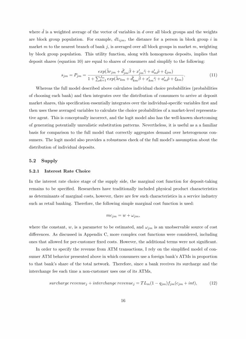
banks’ ATM networks are connected to one another and unaffiliated consumers face fees called

surcharges. I present a structural model of consumer and bank behavior that allows banks to

choose ATM networks and set deposit rates and allows consumers to choose banks. The esti-

mates confirm that network effects are very important in this industry and show that surcharge-

induced incompatibility has a significant impact on demand for deposit services. The results

also suggest that there is overinvestment in ATMs relative to the social optimum. Counter-

factual experiments conditional on network size predict that a move to compatibility through

the elimination of surcharges would substantially decrease market concentration, raise average

deposit interest rates, raise consumer surplus, lower industry profits, and reallocate profits from

large-network banks to small-network banks. Banks are also predicted to respond by reducing

the number of their ATMs.

∗Stanford University Graduate School of Business, Stanford, CA 94305. Email: ishii joy@gsb.stanford.edu. Iam grateful to Ariel Pakes for his advice. I would also like to thank David Blackburn, Eleanor Ericson, KateHo, Catherine Jones, Julie Mortimer, Markus Mobius, Marc Rysman, Minjae Song, and seminar participants at theUniversity of California-Berkeley, Brown, Chicago GSB, Harvard University, MIT, NYU Stern, Northwestern Kellogg,the University of North Carolina Kenan-Flagler, the University of Pennsylvania, Stanford GSB, the University ofWisconsin-Madison, and Wharton.

1 Introduction

This paper examines the effects of incompatibility in network industries. In a network industry such

as telecommunications, the internet, or automatic teller machines (ATMs) in the banking industry,

firms are technologically interconnected. This interconnection can lead to more complicated pricing

structures than those observed in traditional industries, since a consumer may receive direct or

indirect services both from his chosen firm and its rivals. While interconnection increases the size

of the network available to consumers, in industries such as the banking industry, the introduction

of price discrimination between affiliated and unaffiliated consumers reintroduces firm-level network

economies by reducing compatibility within the shared network. This paper measures the impact

of this incompatibility and finds significant effects on competition in the deposit market, welfare,

and investment. It also briefly considers an alternative institutional structure in which provision of

ATM and deposit services is separated.

In the banking industry, the customers of one bank can use their ATM cards at ATMs owned by

other banks, but the ATM owner may charge a fee called a surcharge.1 This can be interpreted as

partial incompatibility between components of a system comprised of ATM cards (bank affiliation)

and ATMs. Analogous to the strong complementary relationships between CPUs and peripherals

or VCRs and video tapes, ATM cards and ATMs form complementary components of a system that

allows consumers to perform transactions on their bank accounts. Consumers can choose various

combinations of these complementary goods, but the compatibility is only partial since there is a

cost associated with use of a foreign ATM, that is, an ATM not owned by the consumer’s bank.

There is a sizeable theoretical literature on compatibility in industries with network externalities

or complementary components.2 This literature predicts that incentives for compatibility differ

across firms and will be smaller for firms with larger networks, since these firms lose the competitive

advantage their network size confers under incompatibility.3 The effects on consumer surplus should

differ depending on the distribution of consumer characteristics and the new price equilibrium that

is reached. In turn, the effects of compatibility on price competition depend on a number of

factors. In the banking industry, while partial incompatibility achieved through surcharging should

theoretically soften price competition in the deposit market by making an increase in deposit1This paper will focus on the types of ATM transactions that can be performed on any ATM within the shared

network such as inquiries and cash withdrawals. According to a study by Dove Consulting (2002), these make up 88percent of all ATM transactions.

2See, for example, Katz and Shapiro (1985) and Farrell and Saloner (1985) for the network externality approach.Matutes and Regibeau (1988) and Economides (1989) introduce models in which there is no consumption externalitybut consumers assemble systems from complementary components.

3For example, Katz and Shapiro (1985) show this effect in their classic model of network externalities, Cremer,Rey, and Tirole (2000) show a similar effect in their model of interconnection quality between internet backbones, andChou and Shy (1993) show that a computer hardware producer’s profit decreases when it increases its compatibilitywith software designed for a rival’s hardware.

1

market share come at the expense of surcharge revenue (see Matutes and Padilla 1994), one might

expect this effect to be swamped by the impact of differing ATM network sizes on banks’ pricing

incentives. For example, banks with small networks may be forced to raise their deposit rates

to remain competitive. The impact of incompatibility on prices, welfare, and the distribution of

market shares is therefore an empirical question. In addition, little is known about how banks’

investment incentives affect the optimality of the network equilibrium.

There has been considerable debate regarding the direction and magnitude of these effects since

the widespread introduction of surcharging in the U.S. in 1996. While various banks and businesses

have emphasized the positive effect of surcharges on ATM deployment, some consumer advocacy

groups, politicians, and small financial institutions have argued that surcharging is an anticompet-

itive practice that threatens the survival of small banks. Calls for government intervention have

ranged from requests for regulation of fee disclosure to demands for a total ban on surcharging.

However, there has been only limited empirical evidence about the effects on the retail banking

industry of the partial incompatibility induced by surcharging.

This paper presents a model of demand, price-setting, and ATM network investment in the

banking deposit market that allows me to analyze the effects of surcharging as well as the impli-

cations of the current equilibrium and alternative institutional structures. I estimate the demand

and cost-side parameters from the model of consumer and firm behavior using standard method

of moments techniques in addition to a new methodology presented in Pakes, Porter, Ho, and

Ishii (2005), the method of moments with inequality constraints. To do this, I use a new data

set that includes ownership and surcharge information for ATMs in the state of Massachusetts. I

combine this with data on consumer characteristics, bank deposits, and bank characteristics. After

estimating the model’s parameters, I find that surcharging has a large impact on bank demand.

A one percent increase in a bank’s surcharge (and hence an increase in the surcharge costs that

a consumer avoids by choosing that bank) results in an average increase of 0.12 percent in that

bank’s demand.

Using the estimates from the banking demand and cost equations, I find that in the current

equilibrium, banks’ direct profits from ATM operations generally do not cover their estimated

ATM costs. This highlights the importance of the effect of ATMs on the deposit market. Indeed,

the demand-stealing effects in the deposit market associated with ATM networks and surcharging

seem to be large enough to cause overinvestment in ATMs. In the observed equilibrium, the average

addition to consumer surplus from a bank’s final ATM is estimated to be smaller than the reduction

in total profits.

Next, I consider counterfactual experiments to measure the impact of surcharge-induced incom-

patibility on market shares, equilibrium prices, and consumer and firm welfare. Holding constant

2

network size, I find that an elimination of surcharges causes average deposit interest rates to rise.

Banks with large ATM networks raise their interest rates and lose market share, and banks with

small networks lower their interest rates slightly and gain market share. The magnitude of these

effects is large. In the Boston banking market, for example, the Herfindahl-Hirschman index is

estimated to fall by about 45 percent upon the elimination of surcharges. These interest rate and

market share effects translate into a sizeable reallocation of profits from large-network banks to

small-network banks with an overall loss of industry profits and an increase in consumer surplus.

However, as one would expect, all banks have an incentive to reduce their network sizes.

This motivates consideration of a market design question. I briefly consider a scenario in which

the provision of ATM and deposit services are separated through the use of a network operator

which charges consumers the cost of operating the network. I find that while this is likely to reduce

consumer surplus, total industry profits are estimated to rise, though by a statistically insignificant

amount, and profits are redistributed away from large-network banks toward small-network banks.

In addition to this paper’s contributions to the literature on network industries, it contributes to

the empirical banking literature by accounting for ATM pricing and network size in estimates of the

demand for deposit services and by developing a structural model that accounts for heterogeneous

firm and consumer characteristics in a flexible way. In particular, the model accounts for the spatial

heterogeneity generated by different consumer and bank branch locations and the heterogeneity in

income levels across different geographic locations. This is important in a retail industry such as

banking. It is also able to accommodate a more natural definition of deposit market shares than

those used in previous research. It allows consumers to have heterogeneous levels of income and

deposits and yields predictions about each bank’s dollar volume of deposits as well as its share of

consumers.

This paper proceeds as follows: the remainder of this section discusses the relationship of this

research to the existing literature. Section 2 discusses some of the important institutional details

and history of the ATM industry. In section 3, I describe and summarize the data that will be

used. Section 4 presents the model of consumer and firm behavior, and sections 5 and 6 describe my

implementation and estimation of it. Section 7 provides estimation results, and section 8 discusses

some implications of the estimates and the results of counterfactual experiments. Finally, section

9 concludes. Additional results are presented in the appendices.

1.1 Literature

This paper relates to the small but growing literature on ATM network competition in the retail

banking industry that has emerged to capture the distinctive features of the industry. Massoud

and Bernhardt (2002) investigate the determinants of ATM pricing in a spatial model. Massoud

3

and Bernhardt (2000) extend this model to allow banks to choose ATM concentration. They find

that banks choose ATM concentrations that are socially excessive. McAndrews (2001) is a related

model that solves for the banks’ ATM price-setting equations, allowing for both surcharges and

foreign fees, fees charged by the consumer’s bank for use of a non-bank ATM. Other theoretical

work has examined pricing incentives for banks versus non-banks where all firms have identical

ATM networks (Croft and Spencer 2003).

There has also been some empirical research on ATM competition and the banking industry.

Most closely related to this paper is the empirical work on surcharging. Hannan, Kiser, Prager, and

McAndrews (2003) examine the determinants of surcharging using a probit regression. They find

that banks with many ATMs are more likely to surcharge, banks in markets with many ATMs are

less likely to surcharge, and banks are more likely to surcharge in states that allowed the practice

early. Prager (2001) investigates the effect of surcharging on small banks by taking advantage of the

fact that prior to 1996, some states allowed ATM networks to maintain prohibitions on surcharging

while others did not. Examining the change in market share of small banks between 1987 and 1995,

she finds no significant difference between surcharging states and non-surcharging states. However,

the study relies on a definition of “small” banks that is based on assets rather than ATM network

size. The author is also unable to observe ATM surcharge levels, so actual fee-setting behavior in

states that allowed surcharging is unknown.

Knittel and Stango (2003) examine the effects of surcharge-induced incompatibility between

parts of the shared network. They use hedonic price regressions to confirm their predictions that

incompatibility between a bank’s ATM cards and foreign ATMs lowers willingness to pay for deposit

accounts and strengthens the link between a bank’s deposit account prices and its network quality

through customer willingness to pay. A structural model is presented in Knittel and Stango (2004).

The authors estimate the parameters of a nested logit demand system for deposit account and ATM

services. They conclude that although incompatibility reduces consumer welfare, the increase in

ATM deployment that followed the widespread introduction of surcharging in 1996 sometimes

completely offsets this welfare reduction. However, the authors do not endogenize the pricing of

deposit account services or the choice of ATM network size. Also, while their paper uses a broad

data set with many observations, it must accommodate missing data in several places. In contrast,

this paper uses a small data set with complete market data for each observation. It also endogenizes

deposit interest rates and considers the implications of banks’ ATM costs on investment.

Finally, Gowrisankaran and Krainer (2003) examine the effects of surcharging using a structural

entry model. However, they do not consider the effect of the bundling of ATM services with banking

deposit services, and each entrant is limited to owning a single ATM.

4

2 Industry Background

When banks first began to introduce ATMs in 1969, the machines were accessible only to customers

of the bank. However, in order to increase convenience and lower costs, financial institutions began

to share ATMs with one another and develop shared ATM networks. This process of sharing and

later, the consolidation of many shared networks and the introduction of the national networks,

eventually led to total technological compatibility. Each depositor’s ATM card could be used at

virtually every ATM. In the early days of ATMs, the machines were installed only in bank branches,

but installation of ATMs on city streets or in other locations such as grocery stores or shopping

malls soon appeared. The former type of ATM is now called an “on-premise” or “in-branch” ATM,

and the latter is called an “off-premise” or “remote” ATM.4

Many of the ATM networks initially banned surcharges by preventing ATM-owning member

institutions from directly charging consumers for the use of their equipment, but these networks

began to come under legal attack in the late 1980s by some network members who claimed that the

surcharge ban constituted price-fixing. By April 1996, 15 states had adopted legislation overriding

network surcharge prohibitions. The national networks, Cirrus and Plus, lifted their bans on April

1, 1996, leading to the widespread introduction of surcharges throughout the U.S.

Since then, debate on the issue has continued. Some have argued that surcharges improve welfare

because they encourage investment in ATM networks. Indeed, ATM deployment has increased since

the introduction of surcharges. According to data from the 2003 EFT Databook, while the period

from 1992 to 1996 saw a 59 percent increase in national ATM deployment, there was a 96 percent

increase between 1996 and 2000. However, others have claimed that the incompatibility induced

by surcharges distorts the deposit market and is welfare-reducing. The U.S. Congress has held

hearings, and there have been attempts to re-ban or otherwise regulate surcharges at various levels

of government. Nevertheless, although the most successful attempts have been at the state and

municipal levels, federal courts have ruled that states and localities do not have the jurisdiction to

regulate the ATM fees of national banks. Two separate federal court rulings in 2002 voided bans

on surcharging in Iowa and in the cities of San Francisco and Santa Monica on these grounds.

Surcharges are the ATM fee on which this paper focuses, but there are other fees that pass be-

tween the consumer’s bank and the ATM owner (the interchange fee) and between the consumer’s

bank and the network (the switching fee). Along with surcharges, the interchange fee provides

compensation to ATM owners for non-customer transactions. The switching fee provides compen-

sation to the shared network for routing non-customer transactions to the customer’s bank. These

fees are not faced by the consumer. In addition, although financial institutions generally do not

charge customers for using their own ATMs, a consumer sometimes faces a foreign fee, a fee set by4See McAndrews (1991) for a review of the history of the creation of shared ATM networks.

5

his own bank for use of ATMs not owned by his bank. I do not directly include foreign fees in the

demand system in this paper, because surcharges are the fees on which the public debate centers,

and I lack data on foreign fees. They tend to be complicated, often being non-linear, and many

banks offer a variety of schedules of foreign fees.

3 Data

3.1 Data Sources

The data set used in this paper is a cross-section from the state of Massachusetts in 2002. It

has been compiled from a number of different sources. The 2002 ATM data was provided by the

Massachusetts Division of Banks. I calculate the total number of ATMs owned by each bank in

each market and classify each one as in-branch or remote. In the analysis below, I use only unique

ATM locations when calculating the size of a bank’s ATM network in order to focus on spatial

factors. I also assign each bank in each market a surcharge level.

Deposit data for each of the inside goods comes from the Summary of Deposits for 2002. This

provides deposits by branch and the addresses of the branches for each commercial bank and thrift.

By geocoding the branches, that is, assigning each a latitude and longitude, I am able to calculate

a bank’s total deposits in a local market. As discussed below, I use credit unions as the outside

good in the demand system, and the Financial Performance Reports of the National Credit Union

Association provide me with credit union deposit data.

I derive additional bank-level data from the Call Reports and Thrift Financial Reports. These

are statements of condition that financial institutions file with the Federal Deposit Insurance Cor-

poration (FDIC) or the Office of Thrift Supervision (OTS), respectively. I estimate the bank-level

deposit interest rate as the ratio of interest expense on deposits to deposits. Similarly, I calculate

the bank-level loan rate as the ratio of revenue on loans and leases to loans and leases. The in-

terest and loan rates are both calculated as six-month rates. I also use the bank’s total number

of branches and employees to calculate employees per branch. Finally, I use several variables to

calculate instruments that will be described in section 6.5

Data on shared network interchange and switching fees are derived from the 2003 EFT Data-

book. I use the average fees in 2002 for NYCE, the main regional shared network for Massachusetts.

These were 46.5c for interchange and 7.75c for switching. Finally, I use information from the 2000

Census for consumer data. This provides me with block group-level information on median income

levels, total population, and the latitudes and longitudes of the area centroids.6 Combining this5The interest and loan rates use expenses or revenues from January through June 2002. The other variables,

including total deposits, loans, and leases, are all calculated as of the end of June 2002.6Block groups are subdivisions of census tracts. They consist of sets of blocks within a census tract having the

6

information with the geocoded locations of the bank branches, I am able to calculate distances from

each block group to each bank branch. Appendix A provides additional details about the data.

3.2 Market Definition and Data Summary

I define a market’s geographic size as a metropolitan statistical area (MSA). The product market is

defined as deposits at depository institutions. Deposits include checking, savings, and time deposits,

and depository institutions include commercial banks, thrifts, and credit unions while excluding

other financial institutions such as mortgage or finance companies. Although credit unions are

a type of depository institution, it would be difficult to model them as one of the inside goods.

Eligibility for participation in a credit union is often idiosyncratic, and for the purposes of my paper,

credit unions are modelled as the outside alternative. Appendix A contains more motivation and

details about the market definition.

These geographic and product-market definitions leave me with a total of 10 markets and

291 bank observations.7 Table 1 provides a brief summary of the markets. They vary in the

number of competitors and market shares. With 148 banks, the Boston market has the largest

number of competitors and the smallest average market share. Pittsfield has the smallest number

of competitors, 8 banks. The market share of the outside good has a substantial range.

Table 2 displays some summary statistics on bank characteristics. The average number of bank

branches is 6.2, and the average number of ATMs is 10.1. These distributions are somewhat right-

skewed, with medians of 3 and 4, respectively. The standard deviation of the number of ATMs is

large, because most banks have moderate numbers of ATMs but a few, such as Fleet or Citizens,

have very large networks. Banks have, on average, 5.7 in-branch ATMs and 4.4 remote ATMs.

However, many banks have no remote ATMs at all: the median is zero. The average number of

employees per branch is 19.2. The interest rate has a mean of 1.2 percent, with a standard deviation

of 0.3 percent.

The distribution of surcharge levels across all banks that own ATMs is shown in Table 3. The

surcharges range from $0 to $2 and move in discrete increments of $0.25 or $0.50. The average

surcharge is $0.78. As was also true in the data used by Hannan, et al. (2003), most of the mass

of the distribution is at $0 and $1. For those banks setting a non-zero surcharge, there is limited

variation, but the overall industry standard is $1. The table also shows that those banks setting

higher surcharges (or, essentially, those banks who surcharge) tend to own larger percentages of the

shared ATM network. This is consistent with the theoretical predictions of Massoud and Bernhardt

same initial digit.7I drop from the analysis two very small banks that offer no ATM services. Also, a few financial institutions listed

in the Summary of Deposits for which depository services are clearly offered only as part of the company’s wealthmanagement services are dropped.

7

(2002) and the empirical results of Hannan et al. (2003).

Consumer characteristics are measured at the block group level. Table 4 summarizes the size

and population of the block groups in each of the markets. As might be expected, the average

area is smaller in the more densely populated markets. With an overall average area of 1.14 square

miles and an average population of 1275, the level of measurement of consumer characteristics is

fairly fine. Averaging over all bank observations and block groups, the mean distance to a bank is

12.56 miles, and this figure is as high as 17.41 miles in the Boston market. In contrast, the median

distance between households and their depository institutions has recently been measured at only

3 miles (Amel and Starr-McCluer 2002). Therefore, distance to bank branches is clearly something

that consumers consider when choosing a bank. In addition, Table 4 shows that the variation across

block groups of average bank distance is substantial: in the various markets, the standard deviation

is usually between one-third and one-half of the mean. Because of the importance of distance to

consumers and the extent of the variation in distances caused by geographic differentiation, it will

be important to develop a model that incorporates this block group-level spatial differentiation.

Averaging over all block groups, median income varies across markets from about $39,000 to

$60,000. The variation across block groups within markets is also quite large. This implies that

it will be useful for the model of consumer behavior to account for the impact of heterogeneous

income levels on both consumer preferences and deposit market shares.

4 Empirical Model

In order to investigate the effects of partial incompatibility in the banking industry through ATM

retail interconnection pricing, I set out a model of consumer and firm behavior. This model seeks

to incorporate the most important aspects of the industry in a way that keeps the burden of

estimation reasonable. It assumes that consumers choose banks to maximize their utility given

their own characteristics and the characteristics of each alternative. Banks are assumed to maximize

profits in a two-stage process with simultaneous moves in each stage. First, they choose the size

of their ATM networks given their expectations about their rivals. Second, they select interest

rates to maximize profits conditional on ATM networks in a Nash equilibrium. The use of an

estimated utility function and an interest rate-setting condition will allow for counterfactual policy

experiments in which consumers reallocate themselves across banks and new pricing equilibria are

computed. The use of a network selection stage also allows investment incentives and the optimality

of the current network equilibrium to be considered.

8

4.1 Consumer Behavior

The model assumes that consumers choose a single bank for depository services. The demand side

of the model therefore follows the discrete-choice literature and adapts the methods proposed by

Berry, Levinsohn, and Pakes (1995) (hereafter referred to as BLP). Some modification of the usual

discrete-choice models is required for an application to retail banking, because the fundamental

quantity variable is a bank’s amount of total deposits rather than its number of customers. The

model will therefore assume that individual consumers are endowed with a level of deposits, and

that each consumer places her deposits in her bank of choice.8 Since individual deposits are not

observed, a simple assumption will be used to relate deposits to consumer observables. Deposit

market shares will be determined by aggregating over the expected deposits of individual consumers.

Although other researchers have modelled demand for depository services as a discrete choice,

this paper is the first to use consumer-level location and demographic data. It is also the first to

use a model that makes direct predictions about a bank’s share of deposits as distinct from its

share of consumers. These two market shares clearly differ when consumers have heterogeneous

deposits, and this distinction will affect the model’s implications. For example, consider two banks

in the same market, where one bank has branches located in a high-income area and the other has

branches in a low-income area. If income is related to deposits but consumers are instead assumed

to have homogeneous deposits, the large increase in deposits induced by an increase in interest

rates by the bank in the high-income area will be rationalized by a high consumer sensitivity to

interest rates, whereas the small increase in deposits induced by the same change in interest rates

by the bank in the low-income area will be rationalized by a low sensitivity. Accurate measurement

of these effects are important when policy experiments are to be considered.

My model specifies a consumer utility function that allows for product differentiation and het-

erogeneous preferences driven by consumer characteristics. I assume that the utility of individual

i for bank j in market m is

Uijm = U(xjm, rjm, ξjm, him, εijm, θ),

where xjm is a vector of observable bank characteristics including ATM network characteristics

determined by each bank’s number of ATMs (n), rjm is bank j’s deposit interest rate, ξjm is a

bank unobservable, him is a vector of observable consumer characteristics, εijm is a consumer-

and bank-specific unobservable, and θ is a vector of parameters to be estimated. Note that him

will account for consumer locations. This allows the model to include geographic information

specific to a consumer-bank combination, similarly to Davis (2001). The inclusion in the model8 The assumption that deposits are not a choice variable is clearly a simplification, but it is made in order to keep

the problem tractable. It is fairly reasonable, since one would expect individual deposits to be driven by transactionneeds and fundamentally by income. It is also a standard assumption in the banking literature.

9

of the structural disturbance, ξ, introduces a traditional simultaneity problem which should lead

to correlation between interest rates and this disturbance term. This endogeneity problem will be

handled below through the use of instruments.

Each consumer chooses the bank that maximizes her utility. Conditional on hi, the set of

consumer unobservables, ε, that leads individual i to choose bank j can be implicitly defined as

Aijm = {ε : U(xjm, rjm, ξjm, him, ε, θ) ≥ maxk U(xkm, rkm, ξkm, him, ε, θ)}, where k indexes banks

in market m. Then if ε has distribution f(ε), the probability that consumer i chooses bank j is

Pjm(him) =∫

ε∈Aijm

f(ε)dε. (1)

Therefore, if h has distribution g(h), bank j’s share of consumers is

qjm = qjm(x, r, ξ, θ) =∫

hPjm(h) g(h)dh. (2)

However, in the banking industry, the primary quantity variable of interest is not the market

share of consumers, but rather the share of deposits. Therefore, the deposit market share will be

the integral over the distribution of consumer characteristics of expected deposits divided by total

market deposits. Denote individual i’s deposits by depi and the joint distribution of h and dep

by g(h, dep). Then if the inside and outside banks in market m are indexed by k = 0, ..., Jm, the

market share of bank j in market m is sjm, where

sjm = sjm(x, r, ξ, θ) =

∫h,dep Pjm(h) dep g(h, dep)dh ddep∑Jm

k=0

∫h,dep Pkm(h) dep g(h, dep)dh ddep

. (3)

4.2 Firm Behavior

4.2.1 Interest Rate Choice

Before discussing the first stage in which banks choose network size, I discuss the second stage in

which interest rates are set. Each commercial bank or thrift in my sample is assumed to set its

deposit interest rate to maximize profits conditional on its ATM network and the networks of its

rivals. These banks take in deposits, which are primarily used to generate revenue through the

funding of various credit instruments. They are therefore multiproduct firms, however, this paper

focuses on the deposit side of the banking industry and does not explicitly model any decisions on

the lending side. Dropping the subscript for market m for ease of notation, bank j’s profit is the

following:

Rj =(lj − rj −mcj)×Dsj(x, r, ξ, θ) + surcharge revenuej+

net interchange revenuej − switching costsj + foreign fee revenuej − ηj ,

10

where the rate bank j receives on loans is lj , its deposit interest rate is rj , its marginal cost is mcj ,

its fixed cost is ηj , and D is total market deposits. This formulation assumes constant marginal

costs of deposit-taking, but the fixed cost term allows for economies of scale. The terms involving

ATM fees are defined below, and it is assumed that ATM transactions have no marginal cost.9

I assume the existence of an interior Nash equilibrium in deposit interest rates. When each

bank maximizes its profits given the interest rates of its competitors, its interest rate satisfies the

following first order condition:

−Dsj+D(lj − rj −mcj)×∂sj(x, r, ξ, θ)

∂rj+

∂

∂rj

(surcharge revenuej+

net interchange revenuej − switching costsj + foreign fee revenuej

)= 0.

(4)

The first two terms of this equation have the usual intuition: by increasing the deposit interest

rate slightly, a bank loses the amount of the increase on all of the deposits it currently has, but it

gains an amount equal to the loan rate net of its interest expense and other costs on its increased

demand. As will be clear when surcharge revenue, net interchange revenue, switching costs, and

foreign fee revenue are defined in equations (12) and (13), the effect embodied in the third term is

that an increase in the deposit interest rate raises a bank’s share of consumers, qj , which decreases

revenue from the first three types of fees and increases revenue from foreign fees.

4.2.2 ATM Network Choice

Moving back to the first stage, each bank simultaneously chooses its ATM network size given its

expectations about its rivals. Bank j’s total profit is

πj = π(yj , nj , n−j , bj , δ) = R(yj , nj , n−j)− (bjδ + νj)nj ,

where R(yj , nj , n−j) denotes the second-stage returns to firm j when its network size is nj , its

rivals’ is n−j , and the vector of all other relevant variables is yj ; bj is a vector of cost shifters; δ are

parameters to be estimated; and νj captures cost differences across banks that are unobserved by

the econometrician but known to the bank. For example, a bank may be able to negotiate favorable

terms with a contractor that maintains the machines’ cash levels.10

Bank j’s expected total profit is

E[π(yj , nj , n−j , bj , δ)|Ij ] = E[R(yj , nj , n−j)|Ij ]− (bjδ + νj)nj , (5)

9 According to industry sources, ATM costs are almost entirely fixed with respect to the number of transactions.See, e.g., Dove (2002).

10 It is also possible to include econometrician measurement error. For example, if πoj (·) = πj(·) + uj,nj , where

πoj (·) is observed profits and uj,nj is measurement error, then all the analysis goes through as long as uj,nj is mean

zero conditional on the instruments introduced in section 6.2.

11

where Ij is the agent’s information set at the time of the decision. Note that there can be prediction

error due to randomness in observed profits that is not known at the time decisions are made. For

example, a bank’s expectation of n−j may differ from the outcome. This expectational error,

denoted ej,nj , is mean zero conditional on the information set by construction, i.e., E(ej,nj |Ij) = 0,

where ej,nj = R(yj , nj , n−j)− E[R(yj , nj , n−j)|Ij ].

I assume that each bank maximizes its expected total profit, but rather than approximating

ATM network size as a continuous variable and taking first order conditions, I use a method

that preserves the discrete, ordered nature of the variable.11 A necessary condition for profit

maximization is that for all banks j, bank j’s expected profit from choosing nj is at least as great

as its expected profit from choosing nj − 1 or nj + 1. This necessary condition is also sufficient

when profits are concave in nj . This turns out to be nearly always true at the estimated parameter

values.12

Therefore, an optimal choice of nj satisfies

E[π(yj , nj , n−j , bj , δ)|Ij ] ≥ E[π(yj , nj − 1, n−j , bj , δ)|Ij ]

E[π(yj , nj , n−j , bj , δ)|Ij ] ≥ E[π(yj , nj + 1, n−j , bj , δ)|Ij ].

From equation (5), this implies the following condition:

E[R(yj , nj , n−j)−R(yj , nj − 1, n−j)|Ij ] ≥ bjδ + νj ≥ E[R(yj , nj + 1, n−j)−R(yj , nj , n−j)|Ij ]. (6)

Note that for each bank, calculation of R(yj , nj − 1, n−j) or R(yj , nj + 1, n−j) involves use of the

structural model to compute a new vector of equilibrium interest rates.

5 Empirical Implementation

Given the full behavioral model above, the empirical specification can now be formulated. The

empirical implementation of consumer preferences and demand is discussed first, followed by the

supply side. To briefly summarize, the demand model will assume that a consumer’s utility from

choosing a bank depends on the bank’s characteristics, the consumer’s characteristics, and char-

acteristics of the bank-consumer combination. On the supply side, the primary specifications for

both the marginal cost of deposit-taking and the cost of an ATM network will be simple constant

functions.11 A continuous first order condition method is considered in section 7 as a robustness check, and it yields similar

results. Pakes, Porter, Ho, and Ishii (2005) discusses alternative estimation strategies including the discrete choicelogit method. It also discusses why traditional ordered choice models such as ordered logit or probit are unfeasible.

12 The results are quite similar when the choice set is expanded to nj +/- 1 and nj +/- 2.

12

5.1 Demand

Preferences

The demand side is estimated using two different functional forms for utility. The primary

specification allows for heterogeneity in both consumer and firm observable characteristics. The

conditional indirect utility function of individual i for banks j = 1, ..., Jm in market m takes the

following form:

Uijm = λdepimrjm + d′ijmβ + x′jmγ + a′mρ + ξjm + εijm. (7)

depim is individual i’s deposits, dijm is a vector of individual-specific branch distance variables for

bank j, xjm is a vector of bank-specific observables including ATM network characteristics, am is a

set of market dummy variables for market m, ξjm is a bank unobservable, and εijm is an individual-

and bank-specific unobservable. The utility of the outside alternative, credit unions, is given the

form

Ui0m = ξ0m + εi0m, (8)

where we can normalize ξ0m to zero.

Included in the first term of the utility function is depimrjm, the interest revenue that individual

i receives at bank j. Since individual deposits are not observed in the data, I relate deposits to

an observable variable, income, with the following simple assumption: depim = αyim. I use the

empirical joint distribution derived from the Census data for geographic location and income.

Since there is no error included in this relationship, it is implicitly assumed that any individual-

level error is averaged out in the block group-level data on income. As noted below, it is helpful

to keep the relationship simple since the deposits variable enters both the utility function and the

share equation.

I include in xjm bank j’s employees per branch, its number of ATMs, and the surcharge cost

variable that will be defined below. Each consumer has a location, which determines his distance

to each bank branch. I assume that the distance a consumer has to travel to reach a bank branch

enters his utility quadratically. Since spatial differentiation is a very important aspect of banking

decisions, the utility function accounts for the consumer’s local geography. Included in dijm is

d1ijm (the distance for consumer i to the nearest branch of bank j), d12ijm, d2ijm (the distance for

consumer i to the second nearest branch of bank j multiplied by a multi-branch-bank indicator),

d22ijm, and onebranch (an indicator for single-branch banks).13 In Appendix C, I allow consumers

to have varying valuations for presence in multiple states, and I find no significant effect.13 Further branch distance variables do not enter significantly. I have also tried including the size of the total

branch network to check that these branch distance variables adequately control for the convenience of the branchnetwork. The coefficient on the added branch network variable is insignificant, and the coefficient on the key ATMnetwork variable, the surcharge variable defined below, is insignificantly different.

13

The bank-specific unobservable, ξjm, accounts for various unobserved aspects of bank quality.

This may include things such as the variety of account offerings, the quality of customer service

training, or bank advertising. It also contains account fees which I do not include in the utility

function since this data is not available for the thrifts in my sample.14 Finally, the consumer-specific

unobservable, εijm, accounts for idiosyncratic preferences such as preferences for community banks.

One would also expect the branch geography near a consumer’s workplace to figure in his bank

choice, but since I do not observe workplace locations, this factor will go into εijm.

The only variable in the utility function that remains to be defined is the surcharge variable in

the xjm vector. This should represent an individual’s utility cost from paying ATM surcharges. I

use a reduced-form representation of the expected cost to a customer of bank j due to surcharges.15

We can denote the percentage of the ATM network owned by bank j as fj and bank j’s surcharge

to non-j customers as cj , and suppose that consumers use a foreign bank’s ATMs in proportion to

that bank’s share of the total network. Then if the number of transactions performed by a customer

of bank j in market m at foreign bank k equals Tfkm, where T is some constant, the surcharge costs

faced by that customer are: T∑Jm

k=1,k 6=j fkmckm = T∑Jm

k=1 fkmckm − Tfjmcjm = tm − Tfjmcjm,

where tm = T∑Jm

k=1 fkmckm. The first summation does not include bank j’s surcharge, because

bank-j customers are exempt from them. tm is a market-specific constant that applies to all

choices, and since it enters utility linearly, it cancels out.16 Taking the negative of the remaining

term and dropping T , we can define as an element of xjm surchjm = fjmcjm, which we expect

to have a positive coefficient. The surchjm variable is a measure of the surcharges a consumer

does not have to pay when she chooses bank j. Although this variable does not capture the price

versus convenience trade-off consumers will face when making decisions about ATM use, it has

the advantage of accounting in a simple way for the consumer’s ex ante knowledge at the time

of choosing a bank about all competitors’ ATM network sizes and surcharges. Since, in reality,

consumers will sometimes walk to a less convenient ATM to avoid a high surcharge or forgo use of

an ATM altogether, this expected surcharge cost variable can be interpreted as a combination of

literal surcharge costs and other losses of utility due to inconvenience.

The ATM network size and surcharge variables defined above are calculated based on the entire

market, with the implicit assumption that consumers travel and experience ATM needs throughout14 One would expect individuals with high deposit levels to have a low sensitivity to these fees, and therefore that

market demand would also be fairly insensitive. Dick (2002) indeed finds that demand elasticities with respect toservice fees are quite low in MSA markets, the type of market I examine.

15 Alternatively, one could explicitly model an additional decision-making stage in which consumers choose ATMsbased on their bank affiliation, ATM prices, and the distribution of all ATMs. Unfortunately, bank- or ATM-leveldata on the demand for ATM transactions is unavailable, so this exercise would be extremely demanding of theexisting data.

16 I assume that tm enters linearly in the utility function for all j = 0, 1, ..., Jm. Otherwise, it would simply go intothe market dummies.

14

the market. This seems reasonable, because the markets are defined based on social and eco-

nomic integration, however Appendix C briefly explores the robustness of the results to the use

of ATM variables that are defined more locally. I also consider the effect of no-surcharging alliances.

Market Shares

In order to be able to analytically integrate over the consumer unobservables, ε, I make the

traditional assumption that the εij ’s are distributed i.i.d. type-I extreme value over individuals

and products. From equations (1), (7), and (8), this means that the probability that individual i

chooses bank j is the following:

Pjm(him) = Pjm(depim, dijm) =exp(λdepimrjm + d′ijmβ + x′jmγ + a′mρ + ξjm)

1 +∑Jm

k=1 exp(λdepimrkm + d′ikmβ + x′kmγ + a′mρ + ξkm). (9)

Bank j’s share of consumers, qjm, follows directly from these probabilities, equation (2), and

the distribution of individual characteristics (deposits and branch distances). In order to calculate

deposit market shares, we need these probabilities as well as the distributions of individual deposits

and characteristics. The assumption above that depim = αyim is particularly convenient here since

the relationship has only one parameter which cancels out of the market share equation. The

market share equation can be calculated from equation (3) as the following:

sjm = sjm(x, r, ξ, θ) =

∫y,d Pjm(y, d) · y · g(y, d) dy dd∑Jm

k=0

∫y,d Pkm(y, d) · y · g(y, d) dy dd

(10)

where

Pjm(yim, dijm) =exp(φyimrjm + d′ijmβ + x′jmγ + a′mρ + ξjm)

1 +∑Jm

k=1 exp(φyimrkm + d′ikmβ + x′kmγ + a′mρ + ξkm)

and φ = λα. It is clear that only φ will be identifiable and not λ or α separately. It should also be

noted that identification does not depend on the use of this simple relationship between deposits

and income. For example, random distributions with multiple parameters that need to be estimated

can be used, and one such specification is explored in Appendix C. However, this increases the

computational burden of estimation substantially.

A Simplification: Logit Demand

It is useful to consider a situation in which consumers have homogenous deposit levels, and

consumer heterogeneity in preferences is restricted to enter the utility function only through the εij

term. These assumptions lead to the logit demand model of McFadden (1974). Such an alternative

utility function can be specified as:

Uijm = λrjm + d′jmβ + x′jmγ + a′mρ + ξjm + εijm,

15

where d is a weighted average of the vector of variables in d over all block groups and the weights

are block group population. For example, d1ijm, the distance for a person in block group i in

market m to the nearest branch of bank j, is averaged over all block groups in market m, weighting

by block group population. This utility function, along with homogenous deposits, implies that

deposit shares (equation 10) are equal to shares of consumers and simplify to the following:

sjm = Pjm =exp(λrjm + d′jmβ + x′jmγ + a′mρ + ξjm)

1 +∑Jm

k=1 exp(λrkm + d′kmβ + x′kmγ + a′mρ + ξkm). (11)

Whereas the full model described above calculates individual choice probabilities (probabilities

of choosing each bank) and then integrates over the distribution of consumers to arrive at deposit

market shares, this specification essentially integrates over the individual-specific variables first and

then uses these averaged variables to calculate the choice probabilities of a market-level representa-

tive agent. This is conceptually incorrect, and the logit model also has the well-known shortcoming

of generating potentially unrealistic substitution patterns. Nevertheless, it is useful as a a familiar

basis for comparison to the full model that correctly aggregates demand over heterogenous con-

sumers. The logit model also provides a robustness check of the full model’s assumption about the

distribution of individual deposits.

5.2 Supply

5.2.1 Interest Rate Choice

In the interest rate choice stage of the supply side, the marginal cost function for deposit-taking

remains to be specified. Researchers have traditionally included physical product characteristics

as determinants of marginal costs, however, there are few such characteristics in a service industry

such as retail banking. Therefore, the following simple marginal cost function is used:

mcjm = w + ωjm,

where the constant, w, is a parameter to be estimated, and ωjm is an unobservable source of cost

differences. As discussed in Appendix C, more complex cost functions were considered, including

ones that allowed for per-customer fixed costs. However, the additional terms were not significant.

In order to specify the revenue from ATM transactions, I rely on the simplified model of con-

sumer ATM behavior presented above in which consumers use a foreign bank’s ATMs in proportion

to that bank’s share of the total network. Therefore, since a bank receives its surcharge and the

interchange fee each time a non-customer uses one of its ATMs,

surcharge revenuej + interchange revenuej = TLm(1− qjm)fjm(cjm + int), (12)

16

where T is a scaling factor, L is the number of consumers in the market, qj is bank j’s share of

consumers, fj is its share of ATMs, cj is its surcharge, and int is the network-wide interchange fee.

Also, since a bank pays out the interchange fee and the switching fee and receives the foreign fee

each time a customer uses a foreign ATM,

interchange costsj + switching costsj − foreign fee revenuej =

TLmqjm(1− fjm)(switch + int− forjm),(13)

where switch is the network-wide switching fee, and forj is bank j’s foreign fee.

This implies the following first-order condition from equation (4) for the Nash equilibrium in

interest rates:

−Dmsjm + Dm(ljm − rjm−w − ωjm)∂sjm(x, r, ξ, θ)

∂rjm− TLmfjm(int + cjm)

∂qjm(x, r, ξ, θ)∂rjm

− TLm(1− fjm)(switch + int− forjm)∂qjm(x, r, ξ, θ)

∂rjm= 0.

(14)

Unfortunately, I don’t observe foreign fees. In order to account for them in the profit function, I

assume a level of $1 for each bank.17 Also, T can be estimated from this equation, but in the actual

estimation, the parameter is not estimated with enough precision to be useful. Therefore, I apply

an estimate of the average number of ATM transactions per period and the percentage of foreign

transactions to calibrate T .18

These assumptions about the value of T and the level of foreign fees are made purely to ensure

that the level of calculated profits due to ATM fees is roughly correct. They can only affect the

demand system through their impact on optimal interest rates, and there will likely be very little

impact through this channel. Since revenues from deposit-taking are metered by dollars of deposits

whereas revenues from ATM transactions depend on numbers of customers, the sheer difference in

scale between these figures limits the influence of direct ATM revenue on interest-rate behavior.19

17 The average foreign fee at banks and savings institutions in 2001 was $1.17 according to the Federal ReserveSurvey of retail fees (Hannan 2002).

18 According to the 2003 EFT Databook, there were 3308 monthly transactions per ATM in the U.S. in 2002.Applying this figure to the total number of ATMs owned by banks in the sample and dividing by total populationyields 12.83 transactions per person in a six-month period. In contrast to the count of ATMs used in all other cases,the total number of ATMs used here includes multiple ATMs owned by a bank in a single location. In addition, a2002 survey of consumers conducted by Pulse found that the total percentage of foreign transactions is approximately25 percent. Thus, since I predict that a bank-j consumer makes T (1− fj) foreign transactions, I find the adjustmentfactor, b, such that T = 12.83b and the total predicted percentage of foreign transactions is 25 percent. This impliesb = 0.28 and T = 3.6. Clearly, this adjustment weights total ATM transactions away from foreign transactions andtowards own-bank transactions.

19 In untabulated results, it can also be seen that the parameters are quite robust to the value of T . E.g., using avalue of T twice as large leaves the cost parameter unchanged to the third digit.

17

5.2.2 ATM Network Choice

In the initial ATM network choice stage of the bank’s problem, the function R(yj , nj , n−j), the

returns to bank j when its network size is nj and its rivals’ is n−j , has now been fully specified,

but the cost of this network remains to be specified. The small size of the data set requires a focus

on parsimonious specifications, so the main specification assumes a constant per-ATM cost of the

network, (δ + νj)nj , where νj is the cost unobservable introduced in section 4.2.2. Alternative

specifications for ATM costs are also considered in Appendix C. Equation (6) then implies that

E[R(yj , nj , n−j)−R(yj , nj − 1, n−j)|Ij ] ≥ δ + νj ≥ E[R(yj , nj + 1, n−j)−R(yj , nj , n−j)|Ij ]. (15)

6 Estimation

Estimation of the behavioral model will implement two major methodologies. First, the demand

and deposit-market cost parameters will be estimated using generalized method of moments (GMM)

with a non-linear optimization routine and simulation methods. Second, the ATM network cost

parameters will be estimated using a new procedure, the method of moments with inequality

constraints. Readers not interested in the econometric details can skip to the results in section 7.

6.1 Demand and Interest Rate Choice

In order to estimate the parameters from the demand model and the cost of deposit-taking, I

assume that the data-generating process satisfies the following covariance restrictions:

E(ξj(θ0)zDj ) = E(ωj(θ0)zS

j ) = 0, 20 (16)

where zDj is a vector of demand instruments, zS

j is a vector of supply instruments, and θ0 is the true

value of the parameter vector. These moments are stacked, and estimation proceeds with GMM.

The parameters are identified using exogenous variation in the distribution of consumer income

and consumer locations relative to bank locations as well as variation across banks and markets in

deposit market shares and bank characteristics.

Because the methods used here are well-understood, I will describe them briefly in this section

and relegate the details to Appendix B. The estimation encounters two difficulties. First, the

market shares are nonlinear functions of ξ. However, they can be inverted to solve for ξ using

the contraction mapping established in BLP, since this contraction mapping is also valid given

the market share in equation (10). Second, there exists no analytic expression for the integrals in

equation (10), so market shares are simulated using s random draws of individual consumers for each20 This notation includes in θ all parameters to be estimated from the demand and interest rate choice model,

including the marginal cost parameters, w.

18

market.21 Then the simulated share of consumers of bank j is qsimj (x, r, ξ, θ) = (1/s)

∑si=1 Pj(yi, di),

and the simulated deposit share of bank j is

ssimj (x, r, ξ, θ) =

∑si=1 Pj(yi, di) depi∑J

k=0

∑si=1 Pk(yi, di) depi

=∑s

i=1 Pj(yi, di) yi∑Jk=0

∑si=1 Pk(yi, di) yi

,

where Pj is defined in equation (10). This implies a simulated version of the moment condition.

Estimating the Logit Demand Model

Estimation of the logit specification of demand is substantially less complicated because the form

taken by the market share allows it to be linearized through a simple transformation. Equation

(11) implies the following expression:

ln(sj)− ln(s0) = λrjm + d′jmβ + x′jmγ + a′mρ + ξjm (17)

The parameters, λ, β, γ, and ρ are estimated with standard linear instrumental variables techniques.

Instruments

These estimation procedures require suitable demand and supply instruments, zD and zS , re-

spectively. We require that elements of zD are uncorrelated with ξ at θ = θ0. Variables in zS

must similarly be uncorrelated with ω. As is traditional in demand analyses, the vector of firm

characteristics, x, is included in the demand instruments. r cannot be included because we expect

interest rates to be endogenous. In order to include instruments for the individual branch distance

variables, I also include d, the vector of variables that averages over consumer branch distances,

weighting by block group population.

Cost-shifters provide another source of demand-side instruments. Firms should account for

costs when setting the interest rate, leading to correlation between these variables and the interest

rate, but many cost-shifters should not be correlated with demand. I include four such variables in

zD: expenses on premises and equipment, other expenses, a credit risk cost variable, and the wage.

The first three of these variables are normalized by assets. Expenses on premises and equipment

and other expenses are both operating cost variables. Premises and equipment expenses include

expenses on utilities, janitorial services, repairs, furniture, etc. Other expenses include legal fees,

postage, deposit insurance assessments, directors’ fees, etc. The credit risk cost variable employed

is provisions for loan and lease losses. Finally, wages are calculated based on the bank’s labor

expenses and the number of employees.22

21 I use 200 random draws of block groups for each market, weighting the probability of drawing a block group byits population.

22 I consider the possibility that expenses on premises and equipment, other expenses, or wage is correlated withthe demand-side unobservable, ξ, by estimating the model without these instruments and examining the correlationsbetween the predicted ξ and each instrument. In each case, the correlations are small and statistically insignificant.

19

The inclusion of a bank’s surcharge cost variable in the demand instruments as part of x

warrants further discussion. Price variables are traditionally thought to be endogenous, and indeed,

I instrument for interest rates throughout the empirical analysis. However, as is evident in Table

3, there is very little variation in surcharge levels. As was found in Hannan et al. (2003), the

surcharging decision is primarily one of whether to surcharge or not, rather than what level to

choose. In addition, I include in the demand equation what I expect to be the primary determinants

of a bank’s surcharge level: market-level dummies and a measure of the bank’s ATM network size.

ATM network size is also included in x, and one might similarly worry about the endogeneity of

this variable. A bank’s ATM investment equation should have predicted market share in it, which

could lead to correlation between ATM network size and the demand unobservable. However, in

many ways this variable is just another product characteristic, and like most demand studies, I

take product characteristics as predetermined. In Appendix C, I provide a robustness check of the

assumption of the exogeneity of ATM network size and the surcharge price variable.

6.2 ATM Network Choice

To estimate the parameters and their confidence intervals from the ATM network choice equation,

I use the methods described in Pakes, Porter, Ho, and Ishii (2005) (hereafter referred to as PPHI).

This paper provides simple techniques for estimation from a set of inequality restrictions given

appropriate instruments. These techniques allow for multiple potential equilibria and endogenous

regressors. Identification of the parameters is based on the condition that a bank’s expected profits

from its observed choice are greater than its expected profits from alternative choices.

We require instruments, zj , such that zj ∈ Ij , the agent’s information set, and the cost unob-

servable is mean zero conditional on the instruments, that is, E(νj |zj) = 0. This condition, with

equation (15), implies that

E[R(yj , nj , n−j)−R(yj , nj − 1, n−j)|zj ] ≥ δ ≥ E[R(yj , nj + 1, n−j)−R(yj , nj , n−j)|zj ].

Then, if g(z) is a positive-valued function of z,

E[(

R(yj , nj , n−j)−R(yj , nj − 1,n−j))g(zj)

]≥ δ g(zj) ≥

E[(

R(yj , nj + 1, n−j)−R(yj , nj , n−j))g(zj)

].

(18)

Each element of g(z) contributes two moments that define an upper and lower bound for δ.

Since banks are interacting agents within a market, to use this restriction in estimation, I create

market-level observations by averaging over banks within markets. Before taking the average over

markets, each market average is weighted by the square root of the number of banks in the market.

This varies significantly across markets, and we expect less noise in the market average for markets

20

having many banks. Let Jm denote the number of banks in markets indexed by m = 1, ...,M . The

sample analogue of the conditions in equation (18) is therefore

1M

M∑m=1

√Jm

Jm

Jm∑j=1

[(R(yj , nj , n−j)−R(yj , nj − 1, n−j)

)g(zj)

]≥ 1

M

M∑m=1

√Jm

Jm

Jm∑j=1

δ g(zj) ≥

1M

M∑m=1

√Jm

Jm

Jm∑j=1

[(R(yj , nj + 1, n−j)−R(yj , nj , n−j)

)g(zj)

].

All δ that satisfy this set of inequalities are included in the feasible set of parameters. If there

exists no such δ, we find the point that minimizes the sum of the absolute value of the amount by

which each inequality is violated.

Confidence intervals are constructed in two different ways as in PPHI. First, I calculate a “con-

servative” (1− α) level confidence interval. This interval is the set of parameters such that, given

the distribution of the sample moments, all moments are satisfied with probability (1 − α). I also

construct an alternative, simulated confidence interval for the parameters. I take simulation draws

from an approximation of the limit distribution of the data and estimate the parameters at each

draw. This provides a simulated distribution of parameters from which confidence intervals can

be directly calculated. PPHI contains additional details on the properties and construction of the

estimator.

Instruments

I use a constant term, market population, the number of banks in a market, and the number of

branches of a bank in a market as z variables to construct instruments. These variables are all in

the information sets of the agents at the time they make their ATM network choices. Furthermore,

they can reasonably be assumed to be independent of the νj cost disturbances in the profit function.

I use simple transformations of these variables as the actual instruments, g(zj). For each element of

zj , I use one indicator function equal to one if zj exceeds its mean, and another indicator function

equal to one if zj is less than or equal to its mean.

7 Results

I first estimate the logit demand model, because this specification is simple to compute and will

provide a basis for comparison to the full model. Then I estimate the full model which integrates

individual demand over the distribution of consumers. Table 5 shows the results of estimating the

logit demand model, where the dependent variable is ln(sj) − ln(s0). The coefficients from OLS

estimation are in the left column, and the IV results are in the right column. The effect of the

endogeneity of the interest rate is immediately evident. The interest rate coefficient becomes larger

21

by a factor of 3 when instruments are used. In the OLS version, we expect there to be a nega-

tive correlation between the demand unobservable and the interest rate that biases the coefficient

downwards. The mean interest rate elasticity implied by this coefficient in the IV specification is

2.49.23 This lies between the mean elasticities estimated by Dick (2002) using a logit model in U.S.

MSA markets (1.49) and all U.S. markets (5.86). In addition to differences in specification and

instrumentation, the differences could result from higher elasticities in Massachusetts MSAs than

in MSAs in the nation as a whole or from the addition of thrifts in my data.

Recalling that surchj represents surcharge costs that a consumer avoids by choosing bank j, the

coefficient on surch is positive in the IV specification, as expected, and is statistically significant.

It implies an average elasticity of 0.123. The number of ATMs is also estimated to enter utility

positively. The quadratic specification for branch distance fits fairly well, but three out of four

coefficients are insignificant at the five-percent level. The signs of the coefficients imply that a

consumer’s utility is decreasing at a decreasing rate in the distance to the nearest and second-

nearest bank branch. The dummy for single-branch banks picks up a large negative effect, and the

coefficient on employees per branch is positive as expected. The fit of these regressions is quite

good. The OLS regression has an R2 of 0.85.

Turning now to the full demand and interest-rate-setting model, the first column of Table 6

displays the results from estimating the demand side alone, and the second column shows the

results of estimating the demand and supply sides jointly. Almost no coefficients achieve statistical

significance when demand is estimated alone. However, as expected, joint estimation of demand

and supply increases the precision of the estimates, making each coefficient significant at the five-

percent level or lower. Each standard error is reduced by joint estimation, and some are reduceed

by a substantial amount. The addition of the supply side does not have a large impact on the

demand coefficients. Indeed, there are no significant differences, which provides support for the

supply-side specification.

The coefficient on the interaction between the interest rate and deposits implies an average

elasticity across banks of 4.20 with a median of 3.62. This is somewhat higher than the average

interest rate elasticity from the logit specification of 2.49. The higher elasticities may result from

the fact that the shares in the full model assign a larger weight to consumers with higher income,

who are predicted to be more sensitive to interest rates because of their larger deposit balances.

Comparing the other coefficients to the logit estimates in Table 5, the coefficients on surch, the

dummy for single-branch banks, and employees per branch are very similar. The biggest difference

is in the branch distance coefficients, where the magnitudes in the full model are much larger than

in the logit model. To investigate this further, the third column of Table 6 presents estimates from23 See Appendix D for details on the calculation of elasticities for both the logit and the full demand model.

22

the full model where the block group-specific distance variables have been replaced by the averaged

versions (d) used previously in the logit specification. It is evident that the model picks up a much

stronger effect from branch distance when distance is measured accurately at the block group level.

The distance coefficients from this alternative specification closely resemble the coefficients from

the logit model. The results using the block group-specific variables also have the sensible property

that the coefficients on distance to the nearest branch have a larger magnitude than the coefficients

on distance to the second nearest branch. It also seems that the coefficient on the number of ATMs

decreases when the model accounts for branch distances accurately at the block group level, but

it remains significant at the five percent level. Overall, the fact that the demand coefficients move

little or in sensible ways from the logit to the full model implies that the full model’s distributional

assumption on deposits is not driving the results. Finally, the marginal cost of deposit-taking for a

six-month interval is estimated to be 1.97 cents per dollar. This coefficient is estimated extremely

precisely.

To illustrate the relative magnitudes of the coefficients, the effect of a one-standard deviation

increase in the interest rate evaluated at the average income in the sample is equivalent to the effect

of an increase in the surcharge variable of 2.8 standard deviations or an increase in the number of

ATMs of 8.5 standard deviations. This same increase in the interest rate is also roughly equivalent

to a decrease in the distance to the nearest bank branch of 1.1 miles or a decrease in the distance

to the second nearest bank branch of 3.4 miles.24

A number of alternative specifications that explore the robustness of these demand- and supply-

side results are considered in Appendix C. I allow consumers’ valuations to depend on bank presence

in multiple states; I use an alternative assumption on the deposit distribution; I generalize the cost

function specification; I examine the potential endogeneity of the surcharge cost variable and ATM

network size; I consider more local definitions of the ATM variables in the demand system; and I

examine the effect of no-surcharge alliances. The primary specification is found to be reasonably

robust.

Finally, Table 7 presents the estimated parameters from the ATM network choice model. The

first row contains the results from the primary cost specification in which there is just a single

constant multiplying the number of ATMs. The estimated parameter is a singleton, i.e., there

exists no set of parameters that satisfy every inequality restriction.25 The estimated constant is

$32,492 for a six-month period, implying an ATM cost per location of about $5415 per month

with a simulated 95 percent confidence interval from $4905 to $6407 per month. As expected, the

conservative confidence interval is wider, ranging from $15,501 to $45,386 for a six-month period,24 These effects are evaluated at the mean branch distance, where the mean is taken over consumers and banks.25 This is not surprising, because the inequalities are random variables. The probability that all elements are

satisfied can be made arbitrarily small by increasing the number of inequality restrictions.

23

which is about $2584 to $7564 per month. Recalling that these figures are based on ATM locations

rather than actual ATM numbers, and using the fact that there are an average of 1.3 ATMs per

location in the data, the average cost per ATM would be 77 percent of the figure above, or about

$4165 per month.26

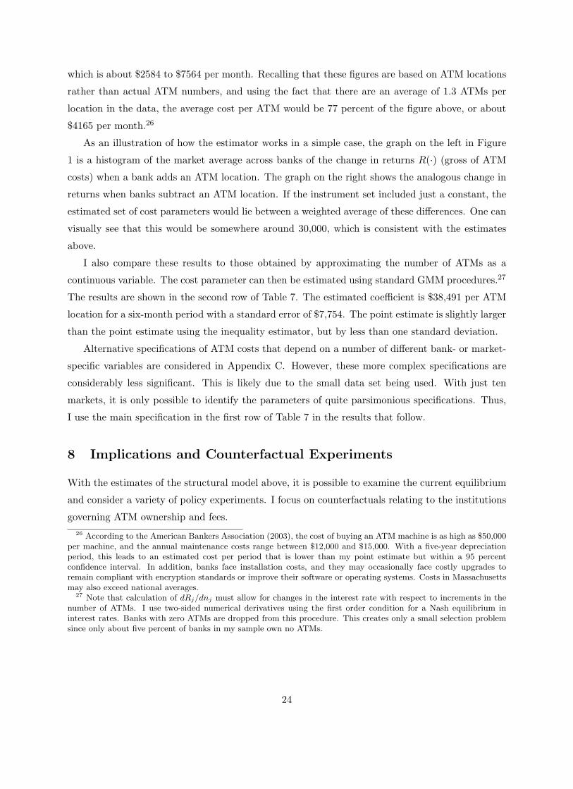
As an illustration of how the estimator works in a simple case, the graph on the left in Figure

1 is a histogram of the market average across banks of the change in returns R(·) (gross of ATM

costs) when a bank adds an ATM location. The graph on the right shows the analogous change in

returns when banks subtract an ATM location. If the instrument set included just a constant, the

estimated set of cost parameters would lie between a weighted average of these differences. One can

visually see that this would be somewhere around 30,000, which is consistent with the estimates

above.

I also compare these results to those obtained by approximating the number of ATMs as a

continuous variable. The cost parameter can then be estimated using standard GMM procedures.27

The results are shown in the second row of Table 7. The estimated coefficient is $38,491 per ATM

location for a six-month period with a standard error of $7,754. The point estimate is slightly larger

than the point estimate using the inequality estimator, but by less than one standard deviation.

Alternative specifications of ATM costs that depend on a number of different bank- or market-

specific variables are considered in Appendix C. However, these more complex specifications are

considerably less significant. This is likely due to the small data set being used. With just ten

markets, it is only possible to identify the parameters of quite parsimonious specifications. Thus,

I use the main specification in the first row of Table 7 in the results that follow.

8 Implications and Counterfactual Experiments

With the estimates of the structural model above, it is possible to examine the current equilibrium

and consider a variety of policy experiments. I focus on counterfactuals relating to the institutions

governing ATM ownership and fees.26 According to the American Bankers Association (2003), the cost of buying an ATM machine is as high as $50,000

per machine, and the annual maintenance costs range between $12,000 and $15,000. With a five-year depreciationperiod, this leads to an estimated cost per period that is lower than my point estimate but within a 95 percentconfidence interval. In addition, banks face installation costs, and they may occasionally face costly upgrades toremain compliant with encryption standards or improve their software or operating systems. Costs in Massachusettsmay also exceed national averages.

27 Note that calculation of dRj/dnj must allow for changes in the interest rate with respect to increments in thenumber of ATMs. I use two-sided numerical derivatives using the first order condition for a Nash equilibrium ininterest rates. Banks with zero ATMs are dropped from this procedure. This creates only a small selection problemsince only about five percent of banks in my sample own no ATMs.

24

8.1 Current Equilibrium

Before considering any counterfactuals, I first examine the implications of the estimated model in

the current equilibrium. Using observed values of all variables and estimated demand and cost

parameters, I evaluate each bank’s total profits. These include profits from the deposit market as

well as from ATM operations.

Many large banks have defended their use of surcharges by noting that ATMs are expensive

to provide, and indeed, not a profit-generating enterprise. For example, Dove (2002) reports that

“aggressive deployment and intense competition have competed away surcharges’ spoils” and re-

sulted in negative ATM profitability for many banks. The president of a small financial institution

explains that “the machines aren’t intended to be a cash cow” but rather a service (Petersen 2002).

This claim is supported in my results. The model predicts that at the observed levels of interest

rates, almost no bank that owns ATMs makes enough revenue directly from its ATM operations to

offset its costs.28 This implies that an important part of a bank’s incentive to own ATMs derives

from their effect on the deposit market. The elimination of surcharges, which provide incentives for

banks to invest in their ATM networks through direct fees as well as indirectly through the deposit

market, may thus have a sizeable impact on the investment equilibrium.

However, this industry has significant potential for an overinvestment problem due to the large

demand-stealing effects in the deposit market associated with ATM networks and surcharging.

When a bank chooses its ATM network size, it does not account for the effect of its choice on its

rivals’ profits. To investigate this, for each bank with positive ATMs, I use the estimated demand

and cost parameters to calculate the change in total profits and consumer surplus associated with

the addition of the bank’s final ATM. I hold the bank’s rivals’ networks fixed and allow for changes

in the interest rate equilibrium. I use the lower bound calculation of consumer surplus described

below in section 8.2 which holds consumers’ choices fixed. Averaging across banks, a lower bound

on the average increase in consumer surplus is $6,886, while total profits decrease by an average

of $60,381. This provides some evidence of overinvestment in this industry relative to the social

optimum.29 This overinvestment result will be mitigated to the extent that the true change in28 Only one bank is predicted to cover its ATM costs through direct ATM revenue.29 One might worry that the change in profits associated with an increase in ATMs is understated here, because it

does not account for a decrease in labor costs due to substitution away from bank tellers. However, according to theOccupational Employment Statistics (OES) from the Bureau of Labor Statistics, the average annual teller wage in mymarkets in Massachusetts in 2002 was $22,517, implying a six-month wage of $11,259. If an additional ATM alloweda bank to hire one less teller, this would therefore raise profits by about $11,259, or less than a fifth of the estimatedchange in profits. However, it is unlikely that even this amount of teller cost savings would be realized, since banksare unlikely to substitute between ATMs and tellers one-for-one. Based on national data from the OES and the 2003EFT Databook, for every additional ATM deployed between 1998 and 2002, banks employed only about 0.2 fewertellers. It is also not the case that banks were shutting down large numbers of branches, since according to the FDIC,the number of banking offices increased by approximately 2 percent during the same period. It is therefore unlikelythat the overinvestment estimate is entirely due to such costs. Another potential source of cost savings due to ATMsmight arise if the convenience of ATMs leads consumers to hold smaller stocks of cash. However, conversations with

25

consumer welfare exceeds the lower bound, but it seems unlikely that the sign of the effect could

be reversed by accounting for switching between banks.30

8.2 Eliminating Surcharges

The possibility of banning surcharges has been at the heart of the public debate about ATMs since

the mid-1990s, and bans were even implemented in certain states and municipalities before being

vacated in court. However, there has been little evidence available regarding the effects of such

bans. I first use the estimated model to predict the effects on market shares, equilibrium interest

rates, and welfare conditional on banks’ ATM networks. Since surcharging is expected to be an

important determinant of a bank’s optimal level of investment in its ATM network, it will not be

possible to draw conclusions from these results regarding the overall welfare effects of surcharging.

Below, I also consider the effect of surcharging on ATM investment incentives.31

After exogenously setting the surcharge cost variables to zero for all banks, consumers are

allowed to reoptimize in their bank choice. The new pricing equilibrium is computed numerically.

Starting at the observed interest rates, I search for the new vector of interest rates at which no

firm can gain profits by deviating. Standard errors are computed using a Monte Carlo approach.

They are based on 200 draws from the estimated asymptotic distribution of the parameters and

their associated policy implications.

Using the estimated parameters from column 2 of Table 6, the results of this experiment on

market shares and prices are shown in Table 8. Allowing banks to adjust their interest rates

and weighting banks’ interest rate changes by their initial deposits, equilibrium deposit interest

rates are predicted to rise by 0.025 percentage points (2.87 percent) on average. These estimates

are significant at the one-percent level. It thus appears that eliminating surcharges intensifies

competition on interest rates. The magnitude of the price effect is fairly small, indicating that

surcharging does not have a huge impact on the deposit rate paid on the average dollar of deposits.

However, this average across banks masks the fact that the size and direction of the effect

depends on the relative size of the bank’s ATM network. Banks with between zero and 10 percent

of the network (“small-network banks”) constitute most of the banks. Interest rates on deposits at

these banks, on average, decrease a small amount, and these banks gain market share. The increase

industry representatives indicate that banks do not consider this to be a significant factor. One bank executive notedthat while ATM networks have expanded considerably over the past five years, the size of the average cash withdrawalhas remained stable.

30 Using the equivalent variation of the change in consumer surplus described in section 8.2, the average estimatedincrease in consumer surplus is smaller than $6,886.

31 This counterfactual experiment assumes that the interchange and switching fees set by the shared networkdo not change. Although surcharges were widely introduced in 1996, network interchange fees generally remainedflat or increased between 1990 and 2002 (see Debit Card Directory, 1995 and 1998, and the EFT Databook, 2003).Therefore, it does not appear that interchange fees have been very sensitive to surcharge levels.

26

in market share is small in absolute value, but is about 25 percent of initial market share. The

largest ATM owners, those with 20 to 30 percent of the shared network (“large-network banks”,

e.g. Fleet, Citizens, Sovereign, or BankNorth), respond to the surcharge ban by raising interest

rates: the interest rate on the average dollar of deposits rises by 7.2 percent. Nevertheless, these

banks’ market share is predicted to fall by an average of 5.6 percentage points, which is 35 percent

of their original market share. The effects at banks with 10 to 20 percent of the ATM network

(“medium-network banks”) lie between the effects at the smallest and largest ATM owners. All

the estimated changes in market shares and interest rates are strongly statistically significant with

the exception of the interest rate changes of small-network banks.

It is interesting to see how much the results are affected by the new pricing equilibrium. In

the last two columns of Table 8 where the experiment is repeated holding interest rates fixed, the

effects are similar. Since the large-network banks are constrained not to raise their interest rates

in response to the change, they are predicted to lose even more market share than in the case in

which interest rates are adjustable.

The effect of the shifts in shares on measures of market concentration is displayed in Table 9.

The first two sets of columns show the one-firm and four-firm concentration ratios [C(1) and C(4)].

They are first calculated using observed market shares, then using the predicted market shares after

surcharges are eliminated and banks adjust their interest rates. On average across markets, C(1) is

21.1 percent, and C(4) is 52.7 percent. Elimination of surcharges has the effect of lowering average

concentration. C(1) falls in all markets but two, and by an average of 3.7 percentage points while

C(4) decreases in all markets, with an average decrease of 7.7 percentage points. The last column

in Table 9 shows analogous statistics using the Herfindahl-Hirschman index (HHI).32 Elimination

of surcharges decreases the HHI in all markets, and the average decrease is 169 points.

Since Table 8 demonstrates that banks with large percentages of the ATMs have, on average,

the greatest decreases in market share, one would expect markets in which banks with large ATM

networks also have large market shares to have the greatest decreases in concentration. Boston,

the market in which the changes in concentration are largest, is in fact the market with the highest

correlation between market share and percentage ownership of the ATM network. Across markets,

this correlation has a large negative correlation that is statistically significant with change in C(1)

(-0.69), change in C(4) (-0.70), and change in HHI (-0.76).

Finally, Table 10 examines the effect of these shifts in market shares, interest rates, and sur-32 The HHI is defined as the sum of the squared market shares multiplied by 10,000, where market shares are

calculated here ignoring credit union deposits. The Justice Department and banking authorities do not use creditunion deposits in their estimates of concentration. In addition, the elimination of surcharges causes a decrease inaggregate demand for the inside goods, increasing estimated market shares for credit unions. This can have a largeimpact on HHI if the market share of the outside good is included. In this case, the behavior of HHI is less consistentacross markets, and the average decrease is 15 points.

27

charges on welfare. Elimination of surcharges leads to a loss of industry profits and a reallocation of

profits from the banks with large ATM networks to those with relatively few ATMs. For example,

small-network banks are predicted to gain a total of $44 million per six months while medium-

network banks lose a total of $11 million and large-network banks lose a total of $93 million. This

implies that the industry overall is predicted to lose about $59 million of profits, which is 12.0

percent of profits. When profits are decomposed into profits from the deposit market and profits

from ATM fees, it can be seen that all types of banks lose profits on ATM fees after the elimina-

tion of surcharges. However, the effect of profits being reallocated from banks with larger ATM

networks to those with smaller networks is entirely due to changes in profits from the deposit mar-

ket. The changes in interest rates and market shares lower profits from deposits by $85 million

for large-network banks and $8 million for medium-network banks, while raising these profits for

small-network banks by $52 million. These estimates are significant at the five- or the one-percent

level with the exception of the total profit changes at small-network banks, since the changes in

profits from the deposit market and ATM fees offset each other.

When interest rates are held fixed, the small-network banks benefit more from the elimination

of surcharges, because the large-network banks are constrained not to raise their interest rates.

This leads to an overall loss of industry profits from deposits of about $31 million per six months.

The total loss of industry profits is estimated at about $49 million per six months, or 9.9 percent.

It is difficult to use this model to estimate consumer surplus, because there is no marginal

utility of income parameter directly estimated as part of the demand system. Therefore, I calculate

a lower bound on the change in consumer surplus defined as the change in transfers from banks

to consumers holding market shares fixed. This is equal to the expected change in deposit interest

received by consumers less the change in surcharges paid when consumers do not reevaluate their

bank choices. This forms a lower bound since consumers may increase their utility by switching

banks.

As displayed in Table 10, this lower bound on the change in average individual consumer surplus

is estimated to be $8.40 per six months when surcharges are eliminated and banks reoptimize their

interest rates. This estimate is statistically significant. Total consumer surplus in the sample of

Massachusetts MSAs rises by an estimated $49.32 million per six months, or $98.64 million per

year. The magnitudes of the consumer surplus effects are considerably smaller when interest rates

are held fixed. Conditional on ATM networks, the estimated change in total welfare is therefore

a statistically insignificant decrease of $10.06 million per six months. The total welfare effect will

be greater to the extent that consumer switching across banks leads to increases in the change in

consumer surplus beyond the lower bound.

A traditional method for estimating the total effect on consumer welfare uses the equiva-

28

lent variation (EV), which is the amount of consumer income that is equivalent to the change

in welfare. For an individual consumer, the EV associated with the elimination of surcharges is

EVi = (1/µ)[maxj Uno surchargesij −maxj U surcharges

ij ], where µ is the marginal utility of income. This

can be aggregated across consumers to produce the total change in consumer surplus.33 To use

this expression, we need an estimate of µ. The coefficient on the expected surcharge costs can be

interpreted as the marginal utility of income multiplied by the constant T , originally defined in

section 5.1. Therefore, I use the estimate of T discussed in section 5.2 to obtain a rough estimate of

marginal utility. An alternative approach would be to extract an estimate of µ from the coefficient

on the product of the interest rate and income, but this would require a great deal of reliance on

the assumed relationship between income and deposits. The estimated change in consumer surplus

is smaller than the lower bound calculated above, so that lower bound is taken to be more reliable

than this approximation of the equivalent variation.34

It is clear, therefore, that surcharge-induced incompatibility has a substantial impact on market

outcomes and the distribution of welfare in the deposit market. As predicted, when compatibility

causes banks with relatively large networks to lose the advantage of their network size, they are

estimated to lose profits while small-network banks gain profits. The industry overall is predicted

to lose profits. Equilibrium prices are affected as well, with small-network banks lowering their

deposit rates slightly and large-network banks raising them. An elimination of surcharges is also

estimated to reduce market concentration and raise consumer surplus.

The analysis has thus far held ATM networks fixed, but we expect banks’ investment incentives

to depend on the ATM fee structure. It would be ideal to calculate the new network equilibrium

after making a market structure change, however we might expect there to be multiple equilibria

problems in a network industry, and finding the correct new equilibrium is a complex task that is

beyond the scope of this paper. Therefore, I simply look at the direction of each bank’s investment

incentives. If the initial equilibrium were still a Nash equilibrium, then for each bank, holding its

rivals’ network sizes fixed, the bank would find it optimal to leave its network size unchanged. Using

the estimated ATM costs, I calculate each bank’s change in profits from dropping one ATM from

its network, accounting for the implied new interest rate equilibrium. Perhaps not surprisingly,

I find that every bank that owns ATMs finds it optimal to reduce its network size. The average33 It is useful to write the conditional utility function as Uij = Uij + εij , where ε is the extreme value unobservable.

Then the total change in consumer surplus is

∆CS = L

ZEVi g(h)dh g(ε)dε = L

Z(1/µ){ln[

JXj=0

exp(Uno surchargesij )]− ln[

JXj=0

exp(Usurchargesij )]}g(h)dh,

where L is the total mass of consumers. The second equality is derived in McFadden (1981).34 Average individual consumer surplus is estimated to rise by $3.22 per six months, and total in-sample consumer

surplus is estimated to rise by $18.90 million per six months.

29

change in profits from a reduction of one ATM is about $29,000 per six months.35

Given this investment response, it is likely that the overall welfare effect from eliminating sur-

charges will change. A reduction in network size is expected to reduce consumer surplus, potentially

by a large amount. However, a reduction in ATM expenditures may lead to an increase in total

industry profits.

8.3 Introducing a Network Operator

An alternative industry structure of interest would place maintenance and operation of the ATM

network in the hands of a third-party operator. Such a solution has been used, for example, in the

electricity industry where a centralized system operator manages the transmission network. Here,

holding the total network size fixed, I consider whether firm profits and consumer welfare would be

improved or worsened if a third-party operator assumed responsibility for the ATM network and

charged consumers exactly the cost of operating the network.

Based on the size of the total network, the total population, and estimated ATM costs, the cost

per consumer to the network operator would be $16.29. I assume each consumer is charged this flat

fee. The change in consumer surplus without this fee should be very similar to the effect described

above when surcharges are eliminated, but it will differ slightly due to changes in the banks’ profit

function, and therefore their interest rate-setting behavior. In the profit function, I set surcharges,

interchange fees, and foreign fees to zero, since there is no longer a need for payments for foreign

transactions, but I assume that banks continue to pay switching fees.

Table 11 shows the estimated changes in interest rates, market shares, and profits. The effects

on interest rates and market shares are similar to the effects when surcharges are eliminated but

banks continue to own the network. Looking at profits, we can see that, due to the high cost

of owning and operating ATMs, total industry profits rise upon the introduction of a network

operator, but the effect is statistically insignificant. However, there are significant distributional

effects. Small-network banks are estimated to gain from this change, but large-network banks lose

profits. For large-network banks, the gain in profits from forgone ATM costs is outweighed by the

substantial loss in the deposit market.

The estimated lower bound change in consumer surplus is a total of $49.02 million, or an average

of $8.35 per consumer. Since this is much less than $16.29, it seems unlikely that consumers would

be better off under this proposed third party network operator.36 This is perhaps not surprising

given the previous result that banks’ direct revenue from ATM operations does not cover their35 This simple analysis does not distinguish between sunk and non-sunk costs. Banks’ incentives to drop ATMs

may be lessened to the extent that many of the costs of ATM investment are sunk.36 The change in consumer surplus is understated because it does not account for switching between banks or the

elimination of foreign fees. It is impossible to extract this foreign fee effect from the utility function. These twoeffects would have to contribute about $8 per consumer to reverse the sign of the total effect.

30

ATM costs. Banks can cover some of these costs with profits from the deposit market due to the

bundling of deposit services and ATM services in the banking industry.

9 Conclusion

This paper has estimated a structural model of demand and supply for banking deposit services

that incorporates ATM networks and retail ATM interconnection pricing. In this industry, each

bank’s ATM cards are technologically compatible with all ATMs in the shared network, but the

use of surcharges leads to partial incompatibility. This implies that demand for a bank’s deposit

services should depend on its ATM network size and its surcharge, since consumers are able to

avoid a bank’s surcharge by choosing that bank. The demand parameters reflect this, showing that

consumers value bank ATM network size and dislike surcharges. Indeed, the results of a model of

ATM network investment imply that banks generally do not cover their ATM costs through direct

ATM fee revenue, which highlights the importance of the deposit market on banks’ ATM network

decisions. Strong demand-stealing effects also appear to lead to overinvestment in ATMs in the

observed equilibrium.

The estimated demand and cost parameters imply that network effects and partial incompat-

ibility can have large impacts on equilibrium prices, market share allocations, and welfare. A

counterfactual policy experiment conditional on network size predicts that surcharging leads to

significantly higher concentration and lower deposit interest rates, with the interest rate effects

being the greatest for large-network banks. It also reallocates market share and large amounts of

profits from deposits from small-network banks to large-network banks and lowers consumer sur-

plus. However, surcharging has a substantial positive effect on banks’ incentives to invest in their

ATM networks. A further counterfactual experiment illustrates that an attempt to move provision

of ATM services into the hands of an independent third-party operator would have distributional

effects on firm profits and would be unlikely to benefit consumers.

This paper leaves open questions regarding the ultimate equilibrium response of ATM network

size to policy stimuli. This is of particular interest in a network industry, making this a useful topic

of future research.

31

Appendix A: Data Details

The Massachusetts Division of Banks requires ATM owners to submit information about the

locations and surcharges of each of their ATMs annually. I calculate a bank’s number of ATMs

in a local market by geocoding the ATMs.37 I also classify ATMs as in-branch or remote based

on whether the addresses match any branch addresses of the ATM owner. I assign each bank in

each market a surcharge level. Surcharges are generally a bank-level decision, and other theoretical

and empirical work has treated them this way.38 In the ATM data, for almost 90 percent of bank

observations, only one surcharge level is used across all ATMs owned in a market by that bank.

For those banks that use more than one surcharge, I use the modal surcharge.

To compute the distances between block groups and bank branches, I use the Haversine formula

from Sinott (1984) for calculating the distance between two points on a sphere.

The credit union deposit data from the Financial Performance Reports of the National Credit

Union Association is available by credit union, rather than by branch location. Therefore, I esti-

mate a credit union’s local market deposits as the fraction of its total deposits that is equal to the

fraction of its branches located in the market.39

Market Definition

I assume that the relevant geographic size of a market is a metropolitan statistical area (MSA).40

Antitrust analysis in banking has traditionally assumed that markets are essentially local, and

there has been substantial evidence in favor of geographically local retail deposit markets. Surveys

consistently show that consumers choose financial institutions very close to their homes and work-

places.41 The median distance of consumers from their depository institutions was 3 miles in the

1998 Survey of Consumer Finances, and 75 percent of consumers were within 8 miles (Amel and

Starr-McCluer 2002). Studies have also documented negative relationships between deposit rates

and concentration across local areas using both recent and older data. See, for example, Heitfield

and Prager (2002) and Berger and Hannan (1989). MSAs provide a convenient and commonly used37I use the Maptitude software package for all geocoding of street addresses.38E.g., Hannan et al. (2003), Massoud and Bernhardt (2000,2002), and McAndrews (2001).39This should be a reasonable approximation, and furthermore, in the logit demand specification, any errors in

measurement of market-level demand for credit unions affect only the market dummies. This can be seen in equation(17), in which the share of the outside good affects only the constant subtracted from the left-hand side.

40An MSA is essentially an area with a large population center combined with adjacent communities that are highlysocially or economically integrated. In large markets, I use primary MSAs rather than the larger consolidated MSAs.

41 Although both households and businesses consume banking services, this paper uses a behavioral model ofindividual consumers, since it uses data on household location and demographics. Separation of business fromhousehold demand is often impossible in any demand model. In this application, a model of household behavior isa reasonable simplification, because households hold the vast majority of deposits. According to the 2000 FederalReserve Flow of Funds, households hold about 80 percent of total U.S. household/nonfinancial business deposits. Inaddition, consumer and small business behavior has been found to be similar in the use of depository institutionsand the clustering of demand for financial services at local institutions (Kwast, Starr-McCluer, and Wolken 1997).

32

local geographic delineation.

The product market is defined as deposits at depository institutions, where deposits include

checking, savings, and time deposits. Geographically disaggregated data on branch deposits is

available only for total deposits. Fortunately, there is evidence that consumers cluster their demand

for depository services at their primary institution. According to the 1998 Survey of Consumer

Finances, most households obtain multiple services at their primary financial institution (Amel and

Starr-McCluer 2002). Account balances also tend to be fungible across different types of accounts.

For example, many banks offer “relationship” accounts that link balances across deposit accounts.

Depository institutions include commercial banks, thrifts, and credit unions. Many empirical

banking papers have included only commercial banks in their market definitions, but thrifts and

credit unions have a significant presence in Massachusetts with 16.6 percent of the deposits in

all markets. It is also useful to use this fairly broad definition because, in the behavioral model,

I assume that all consumers use a commercial bank, thrift, or credit union. The 1998 Survey

of Consumer Finance showed that over 98 percent of households with any bank-type accounts

or loans used a depository institution, so this is a reasonable approximation (Amel and Starr-

McCluer 2002). While antitrust analysis has traditionally included only commercial banks in

market concentration calculations, it has accounted for competition from thrifts, credit unions,

and other institutions through the use of merger guidelines that are less restrictive than those

used in non-banking industries.42 Since legislation in 1980 has allowed for increased competition

between commercial banks and thrifts, the Federal Reserve Board now includes some or all thrifts

in their market concentration calculations, while maintaining the relaxed concentration standards

to account for competition from credit unions and other institutions (Amel 1997).

Appendix B: Estimation Details for Demand and Interest Rate Choice

Stacking the covariance restrictions in equation (16), the following moment condition can be

formed:

G(θ) = E[mj(θ)] = E

ξj(θ)zDj

ωj(θ)zSj

.

The vector of demand parameters can be estimated using the demand moments alone. However,

joint estimation using the demand and supply moments is expected to increase the efficiency of the

demand estimates, since the interest-rate-setting equation implied by the Nash equilibrium depends

on the demand parameters. I will estimate θ0 both ways. Equation (16) implies that G(θ0) = 0. If42The U.S. Department of Justice Merger Guidelines state that a proposed banking merger would not be expected

to raise antitrust concerns unless it increased the Herfindahl-Hirschman index (HHI) by 200 or more points and ledto a level greater than 1800. In non-banking industries, mergers that raise the HHI by more than 50 points areconsidered potentially problematic.

33

there are a total of N bank observations in the sample, a sample moment condition can be formed

as follows:

GN (θ) =1N

N∑j=1

mj(θ) =1N

N∑j=1

ξj(θ)zDj

ωj(θ)zSj

.

Under some technical conditions, the estimator defined by minimizing ‖GN (θ)‖A, where A

is a weight matrix, is√

N -consistent and asymptotically normal with variance-covariance matrix

(Γ′AΓ)−1Γ′AV AΓ(Γ′AΓ)−1, where Γ = ∂G(θ0)/∂θ and V = E[m(θ0)m(θ0)′]. These standard errors

allow for arbitrary heteroskedasticity.

The two difficulties that will be discussed in turn are that the market shares are nonlinear

functions of ξ, and the expression for market share is non-analytic. First, individual consumer

demand, and therefore aggregated market demand, is a nonlinear function of the unobservable, ξ.

In order to use the orthogonality restrictions above, it is necessary to transform the data into a

linear function of the ξ. Berry (1994) shows the conditions under which a unique mapping from

shares to ξ exists, given the observable data and the parameter vector, and BLP demonstrates how

this mapping can be computed. In BLP, a contraction mapping is established that allows ξ to be

computed iteratively for each set of parameters, observable data, and distributions of consumer

unobservables. It can be shown that the contraction mapping used in BLP is also a contraction

mapping given the market share in equation (10).43 This should not be surprising given that the

market share used here differs from the standard market share only in that it is a weighted average

of individual consumer choice probabilities, whereas the standard market share is a simple average.

Therefore, the market shares here can be inverted to solve for ξ using the BLP contraction mapping.

Second, it is not possible to explicitly compute GN (θ), because there exists no analytic expres-

sion for the integrals in equation (10), the market share. However, simulation methods as in Pakes

and Pollard (1989) and BLP allow θ to be estimated consistently and with only minor changes in

its limiting properties. The shares are simulated as described above in section 6.1. The asymptotic

distribution of the estimator is affected only through the estimated variance-covariance matrix of

the moment conditions, V , which uses the simulated moments.

In the actual estimation, γ and w are “concentrated out” using the fact that the first-order

conditions associated with the minimization problem are linear in these parameters. Then a non-

linear search is performed over the remaining parameters using the Nelder-Mead non-derivative

simplex method.

Appendix C: Robustness

This appendix considers a number of alternative specifications to explore the robustness of both43 Each of the conditions of the proof in the appendix of BLP can be verified.

34

the demand- and the supply-side results of section 7. First, I examine the demand and interest-

rate-setting model. I allow consumers’ valuations to depend on whether banks have branches in

multiple states; I use an alternative assumption on the deposit distribution; I use a different cost

function specification; I consider the potential endogeneity of the surcharge cost variable and ATM

network size; I consider the possibility that ATM demand is more properly measured at a local

level; and I examine the effect of no-surcharge alliances. I also consider alternative specifications

for the ATM network investment model. I allow the costs of in-branch and remote ATMs to differ;

I consider the possibility that ATM costs depend on the cost of leasing space; and I allow ATM

costs to depend on the size of the network.

First, consumers could have heterogeneous preferences for “large” banks, with some consumers

preferring them and others preferring community-style banks. In column 1 of Table 12, I reestimate

the full model with the addition of a random coefficient on an indicator variable for banks that

have branches in multiple states. I assume that the marginal utility of this variable is distributed

normally across consumers, and I estimate the mean and standard deviation of this distribution.

Neither parameter is estimated to be significantly different from zero.

Next, it was noted previously that it is possible to use more complex assumptions on the

distribution of deposits than the assumption used above. In order to allow randomness in the

distribution, I reestimate the full model assuming that, conditional on yi, deposits are distributed

exponential with mean αyi.44 Column 2 of Table 12 shows the estimated coefficients. They are

qualitatively similar to the main results of Table 6’s second column, though the addition of noise

at the block group level seems to make it harder for the effect of the branch distance variables to

be picked up. Their coefficients are much smaller and less significant. Nevertheless, these results,

combined with the logit results where it is assumed that consumers are homogeneous, provide

evidence that assumptions about the distribution of deposits are not driving the results.

I next examine the cost function. The specification in section 7 included only a constant,

but one might expect there to be not only a marginal cost for deposits but also a fixed cost per

customer due to costs of printing bank statements, providing customer service, etc. The model

can accommodate such costs since it yields predictions for both share of deposits (sj) and share of

consumers (qj). Column 3 of Table 12 shows the coefficient estimates from the full model when the

cost function includes both a constant on deposits and a per-customer fixed cost. The fixed cost

estimate is insignificantly different from zero.

I now return to the issue of the potential endogeneity of the surcharge cost variable or of ATM

network size. It can be argued that there is only minimal variation in surcharges, mitigating the44 Note that this specification once again identifies φ = λα, where λ is the parameter in the utility function on the

product of deposits and the interest rate. One way to see this is by inverting the cdf of the exponential distributionso that if wi = −αyiln(1− ui) where ui ∼ U [0, 1], then wi has the same distribution as deposits, exponential(αyi).

35

scope of the surcharge endogeneity problem. In addition, the observables in the utility function

include what are expected to be the most important determinants of surcharge levels. However,

to address any remaining concerns with the surcharge variable or the number of ATMs, I estimate

the full model again, this time instrumenting for surcharge costs and the number of ATMs. With

the exception of these two variables, I use the same instruments as before, and I add two new

instruments: the number of in-branch ATMs and the number of in-branch ATMs as a percentage

of total market ATMs. In-branch ATMs are highly correlated with total bank ATMs, but they

should be closer to exogenous themselves. Many banks automatically invest in ATM machines

for their bank branches, so if the branch network can be taken as exogenous for the purposes of

this cross-sectional study, then these in-branch ATMs are close to exogenous. Also, they make an

attractive instrument, because a bank’s number of in-branch ATMs may contain information about

the bank’s ATM costs.45

Column 4 of Table 12 presents the results using the full model with demand estimated jointly

with supply. The standard errors on the surcharge cost variable and the number of ATMs increase

when these variables are not included in the instrument set, but the coefficient on surcharge costs

remains significant at the 5 percent level and the coefficient on the number of ATMs is significant at

the 10 percent level. The coefficients are very similar to the results in Table 6, where the surcharge

and ATM network size variables are included in the instrument set. Indeed, none of the coefficients

are significantly different. This provides further support for not instrumenting for the surcharge or

ATM network size variables.

Next, although I expect market-level ATM networks to be a good proxy for what consumers care

about, I consider a local version of this variable. I define an alternative ATM network size variable

as the number of ATMs within a five-mile radius of a consumer’s block group (called #ATMs5).

Similarly, I define a local version of the surcharge cost variable analogous to surch for costs within

a five-mile radius (called surch5). In order to ease the computational burden, I return to the logit

demand model. Column 1 of Table 13 shows the estimated demand coefficients when these ATM

network size and surcharge cost variables are averaged over block groups, weighting by block group

population. Most of the coefficients change very little, but the coefficient on surch5 is smaller

(though not significantly so) and less significant than the coefficient when market-level variables

are used. The change in the ATM network size coefficient reflects the scaling of the variable. Since,

if anything, the coefficient on the surcharge cost variable picks up less of an effect when measured

locally, I maintain the assumption that ATM networks are appropriately measured at the level of

the market. The market-level variables should account for work, shopping, and other important

locations away from home.45In-branch ATMs are thought to be less expensive to install and operate than remote ATMs. See, for example,

Balto (1996) and Dove Consulting’s 2002 ATM Deployer Study.

36

A final potential issue with the estimated demand system is that many banks in Massachusetts

are members of a no-surcharging alliance called SUM. Banks that choose to join SUM agree not

to surcharge each other’s customers, though they still independently set surcharges for customers

of banks that are not members. I therefore consider an alternative surcharge variable called sur

which accounts for the SUM alliance.46 In each market m, the banks can be ordered so that banks

1, ..., Jm are members of SUM and banks Jm +1, ..., Jm are not. Customers of non-SUM banks face

surcharge costs of tm−Tfjmcjm, as above, whereas customers of SUM banks should face surcharge

costs of T∑Jm

k=Jm+1fkmckm = T

∑Jmk=1 fkmckm − T

∑Jmk=1 fkmckm = tm − T

∑Jmk=1 fkmckm. As with

surch, the constant, tm, cancels. Therefore, we can define

surjm = I{non-SUM}jmfjmcjm + I{SUM}jm(∑Jm

k=1 fkmckm).

It will also be useful to define the following variables:

surnon−SUMjm = I{non-SUM}jmfjmcjm

surSUMjm = I{SUM}jm

∑Jmk=1 fkmckm

surnojSUMjm = I{SUM}jm

∑Jmk=1,k 6=j fkmckm.

Using a logit regression and the alternative surcharge variable, sur, the second column of Table

13 shows that the coefficients on all variables except for sur appear quite similar to the instrumental

variables results in Table 5. The coefficient on sur is very small and completely insignificant. The

specification in the third column of Table 13 allows for different coefficients on sur for SUM and

non-SUM banks. The coefficient is again small and insignificant for the SUM banks, but is larger

and marginally significant (with a p-value of 0.06) for the non-SUM banks. This difference in

coefficients may arise if consumers do not fully internalize the effect of SUM membership when

choosing banks, so that avoiding surcharges at an ATM in the SUM alliance not owned by the

consumer’s bank is not considered to be equivalent to avoiding surcharges at ATMs owned by

the consumer’s bank. The surcharge variable sur (or surSUM ) would then be mismeasured for

SUM banks. Such an effect could arise if consumers are ill-informed about the SUM alliance when

choosing banks. For example, in 2002, consumers may not have understood how it works, or they

may not have known how large it was or which banks were members.47

To examine this issue further, I consider one additional specification in the fourth column.

This specification splits the terms in surj in a different way. As defined above, surch accounts

for the surcharges of the consumer’s own bank, and surnojSUM handles the remaining terms for

the SUM banks. There is little change in the other coefficients, and the coefficient on surnojSUM

46 Banks are assumed to be members of SUM if they were listed as participating institutions in May 2003 on theSUM website, http://www.sum-atm.com.

47 Indeed, individual banks may not wish to spend significant resources advertising the SUM network, since adver-tising for the network is a form of advertising for their competitors.

37

is insignificantly different from zero. These results imply that the expected surcharge costs at a

consumer’s own bank have a significantly positive effect on bank demand, but the surcharge costs

of SUM banks other than the consumer’s own bank have an insignificant effect. In the analysis,

I therefore use surch in the vector of bank characteristics rather than the alternative surcharge

variable, sur.

I now consider some alternative specifications for the ATM network choice model. I first consider

allowing a different cost coefficient for in-branch and remote ATMs by allowing banks to make

discrete choices over two variables: the number of in-branch ATMs and the number of remote

ATMs. One might expect the cost of installing and maintaining ATMs to be higher for remote

than in-branch ATMs, since rental costs may be higher at remote locations and off-site ATMs may

also be more difficult to service. However, banks may tend to install more ATMs or more expensive

ATMs in their branch locations, so the direction of the cost difference is not clear. Rows 1 and 2

of Table 14 show that the estimated parameters are quite similar, with an in-branch coefficient of

$36,649 and a remote coefficient of $38,348. The remote coefficient is somewhat larger than the

in-branch coefficient, but the remote parameter’s 95 percent confidence interval is also quite a bit

larger. It covers the entire confidence interval for the in-branch parameter in both the conservative

and simulated confidence interval cases.

Next, one might expect ATM costs to vary based on the cost of leasing space. I assume that

the cost of an ATM network of size nj is (δ+bjδb +νj)nj , where bj is the rental cost variable. Since

commercial real estate price data is unavailable, I use business density as a rough proxy for these

rental costs. The number of firms figure that is used to form this variable is obtained from the 1997

Economic Census, and I include business density in the instrument set for this specification. Rows

3 and 4 show that the coefficient on the business density term is not of the expected sign, and it

is insignificantly different from zero based on the conservative confidence interval. The coefficient

on the constant term is larger than in the primary specification, but its confidence interval is also

much larger. The conservative confidence interval extends past zero.

Finally, I consider a specification that allows the cost per ATM to depend on the size of the ATM

network. I estimate separate coefficients on the number of ATMs and the square of the number of

ATMs. One might expect there to be decreasing costs if owners of larger networks purchase their

machines at lower prices, but there may be offsetting quality differences. In addition, it is possible

that banks face increasing costs as low-cost locations are filled up. Rows 5 and 6 show positive

coefficients for both the number and the square of the number of ATMs. However, the coefficient

on the number of ATMs is no longer significant. This is likely due to the very high correlation

between the number of ATMs and its square (0.96).

38

Appendix D: Elasticity Calculations

In the logit model, in which market shares are as defined in equation (11), the elasticity of bank

j’s share with respect to the interest rate of bank k in market m can be computed as follows:

ηjkm =∂sjm

∂rkm

rkm

sjm=

λrjm(1− sjm) if k = j,

−λrkmskm otherwise.

In the full model, in which market shares are as defined in equation (10), the elasticities take the

following form:

ηjkm =∂sjm

∂rkm

rkm

sjm=

φrjm ×∫y,d Pjm(y, d)[1− Pjm(y, d)] y2 g(y, d) dy dd∫

y,d Pjm(y, d) y g(y, d) dy ddif k = j,

−φrkm ×∫y,d Pjm(y, d)Pkm(y, d) y2 g(y, d) dy dd∫

y,d Pjm(y, d) y g(y, d) dy ddotherwise.

References

[1] Amel, Dean F., 1997, Antitrust Policy in Banking: Current Status and Future Prospects,Conference on Bank Structure and Competition, 33, 166-179.

[2] Amel, Dean F., and Martha Starr-McCluer, 2002, Market Definition in Banking: RecentEvidence, The Antitrust Bulletin, 47(1), 63-89.

[3] American Bankers Association, 2003, ATM Fact Sheet.

[4] ATM and Debit News EFT Databook, 2003 edition, Thomson.

[5] Balto, David A., 1996, ATM Surcharges: Panacea or Pandora’s Box?, Review of Banking andFinancial Services, 12(17), 169-177.

[6] Berger, Allen N., and Timothy H. Hannan, 1989, The Price-Concentration Relationship inBanking, Review of Economics and Statistics, 71(2), 291-299.

[7] Berry, Steve T., 1994, Estimating Discrete-Choice Models of Product Differentiation, RANDJournal of Economics, 25(2), 242-262.

[8] Berry, Steve, James Levinsohn, and Ariel Pakes, 1995, Automobile Prices in Equilibrium,Econometrica, 63(4), 841-890.

[9] Chou, Chien-fu, and Oz Shy, 1993, Partial Compatibility and Supporting Services, EconomicLetters, 41, 193-197.

[10] Cremer, Jacques, Patrick Rey, and Jean Tirole, 2000, Connectivity in the Commercial Internet,Journal of Industrial Economics, 48(4), 433-472.

39

[11] Croft, Elizabeth W., and Barbara J. Spencer, 2003, Fees and Surcharging in Automatic TellerMachine Networks: Non-Bank ATM Providers versus Large Banks, N.B.E.R. Working Paper9883.

[12] Davis, Peter, 2001, Spatial Competition in Retail Markets: Movie Theaters, Working Paper,MIT Sloan.

[13] Debit Card Directory, 1995 edition, 1998 edition, Faulkner and Gray.

[14] Dick, Astrid A., 2002, Demand Estimation and Consumer Welfare in the Banking Industry,Working Paper, Federal Reserve Board, Washington, D.C.

[15] Dove Consulting, 2002 ATM Deployer Study, Executive Summary, February 2002.

[16] Economides, Nicholas, 1989, Desirability of Compatibility in the Absence of Network Exter-nalities, American Economic Review, 1165-1181.

[17] Farrell, Joseph, and Garth Saloner, 1985, Standardization, Compatibility, and Innovation,RAND Journal of Economics, 16(1), 70-83.

[18] Gowrisankaran, Gautam, and John Krainer, 2003, The Welfare Consequences of ATM Sur-charges: Evidence from a Structural Model, Working Paper, Washington University.

[19] Hannan, Timothy H., Elizabeth K. Kiser, Robin A. Prager, and James J. McAndrews, 2003,To Surcharge or Not to Surcharge: An Empirical Investigation of ATM Pricing, Review ofEconomics and Statistics, 85(4), 990-1002.

[20] Hannan, Timothy, 2002, Retail Fees of Depository Institutions: 1997-2001, Federal ReserveBulletin, 405-413.

[21] Heitfield, Erik, and Robin A. Prager, 2002, The Geographic Scope of Retail Deposit Markets,Working Paper, Federal Reserve Board, Washington, D.C.

[22] Katz, Michael L., and Carl Shapiro, 1985, Network Externalities, Competition, and Compati-bility, American Economic Review, 75(3), 424-440.

[23] Knittel, Christopher, and Victor Stango, 2003, Compatibility and Pricing with Indirect Net-work Effects: Evidence from ATMs, Working Paper, Federal Reserve Bank of Chicago.

[24] Knittel, Christopher, and Victor Stango, 2004, Incompatibility and Consumer Demand: Evi-dence from ATMs, Working Paper, UC Davis.

[25] Kwast, Myron L., Martha Starr-McCluer, and John D. Wolken, 1997, Market Definition andthe Analysis of Antitrust in Banking, The Antitrust Bulletin, 42(4), 973-995.

[26] Massoud, Nadia, and Dan Bernhardt, 2000, Endogenous ATM Concentration, Working Paper,University of Alberta.

[27] Massoud, Nadia, and Dan Bernhardt, 2002, ATM Competition: Understanding “Rip-Off”ATM Surcharges, RAND Journal of Economics, 33(1), 96-115.

[28] Matutes, Carmen, and Jorge A. Padilla, 1994, Shared ATM Networks and Banking Competi-tion, European Economic Review, 38(5), 1113-1138.

40

[29] Matutes, Carmen, and Pierre Regibeau, 1988, “Mix and Match”: Product CompatibilityWithout Network Externalities, RAND Journal of Economics, 19(2), 221-234.

[30] McAndrews, James J., 1991, The Evolution of Shared ATM Networks, Business Review, Fed-eral Reserve Bank of Philadelphia, 3-16.

[31] McAndrews, James J., 2001, A Model of ATM Pricing: Foreign Fees and Surcharges, WorkingPaper, Federal Reserve Bank of New York.

[32] McFadden, Daniel, 1974, Conditional Logit Analysis of Qualitative Choice Behavior, in P.Zarembka, ed., Frontiers in Econometrics, 105-142, New York: Academic Press.

[33] McFadden, D., 1981, Econometric Models of Probabilistic Choice, in C. Manski and D. Mc-Fadden, eds., Structural Analysis of Discrete Data, 198-272, Cambridge: MIT Press.

[34] Pakes, Ariel, and David Pollard, 1989, Simulation and the Asymptotics of Optimization Esti-mators, Econometrica, 57(5), 1027-1057.

[35] Pakes, Ariel, Jack Porter, Katherine Ho, and Joy Ishii, 2005, Moment Inequalities and TheirApplication, Working Paper, Harvard University.

[36] Petersen, Rebecca A., Automatic Fees, Ames Tribune, May 28, 2002.

[37] Prager, Robin, 2001, The Effects of ATM Surcharges on Small Banking Organizations, Reviewof Industrial Organization, 18(2), 161-173.

[38] Sinnott, Roger W., 1984, Virtues of the Haversine, Sky and Telescope, 68(2), 159.

41

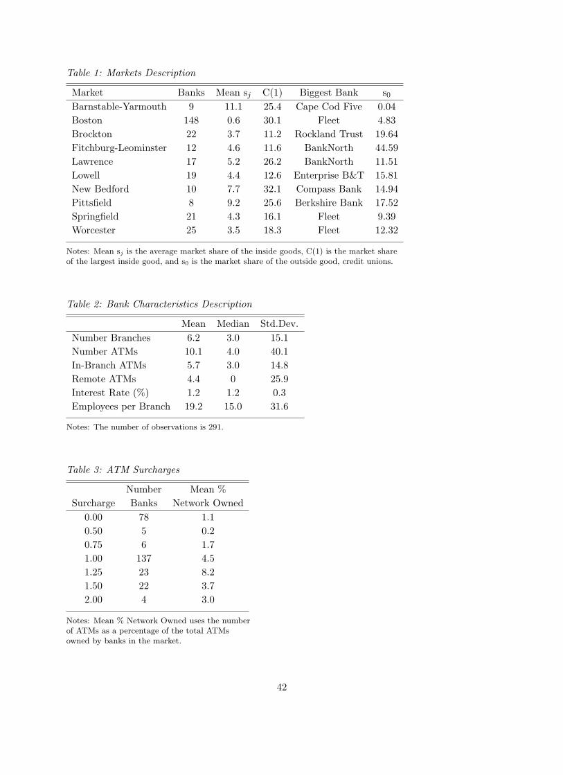
Table 1: Markets Description

Market Banks Mean sj C(1) Biggest Bank s0Barnstable-Yarmouth 9 11.1 25.4 Cape Cod Five 0.04Boston 148 0.6 30.1 Fleet 4.83Brockton 22 3.7 11.2 Rockland Trust 19.64Fitchburg-Leominster 12 4.6 11.6 BankNorth 44.59Lawrence 17 5.2 26.2 BankNorth 11.51Lowell 19 4.4 12.6 Enterprise B&T 15.81New Bedford 10 7.7 32.1 Compass Bank 14.94Pittsfield 8 9.2 25.6 Berkshire Bank 17.52Springfield 21 4.3 16.1 Fleet 9.39Worcester 25 3.5 18.3 Fleet 12.32

Notes: Mean sj is the average market share of the inside goods, C(1) is the market shareof the largest inside good, and s0 is the market share of the outside good, credit unions.

Table 2: Bank Characteristics Description

Mean Median Std.Dev.Number Branches 6.2 3.0 15.1Number ATMs 10.1 4.0 40.1In-Branch ATMs 5.7 3.0 14.8Remote ATMs 4.4 0 25.9Interest Rate (%) 1.2 1.2 0.3Employees per Branch 19.2 15.0 31.6

Notes: The number of observations is 291.

Table 3: ATM Surcharges

Number Mean %Surcharge Banks Network Owned

0.00 78 1.10.50 5 0.20.75 6 1.71.00 137 4.51.25 23 8.21.50 22 3.72.00 4 3.0

Notes: Mean % Network Owned uses the numberof ATMs as a percentage of the total ATMsowned by banks in the market.

42

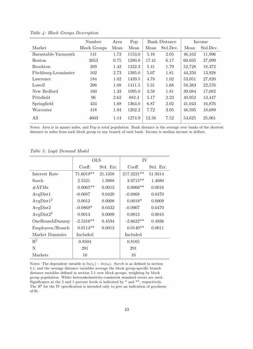
Table 4: Block Groups Description

Number Area Pop Bank Distance IncomeMarket Block Groups Mean Mean Mean Std.Dev. Mean Std.Dev.Barnstable-Yarmouth 141 1.73 1153.0 5.16 2.05 46,342 11,996Boston 2653 0.75 1280.8 17.41 6.17 60,035 27,099Brockton 209 1.42 1222.3 5.41 1.79 52,728 18,372Fitchburg-Leominster 102 2.73 1395.0 5.07 1.81 44,250 13,928Lawrence 184 1.02 1439.5 4.78 1.02 53,051 27,820Lowell 206 1.08 1411.5 5.31 1.68 58,383 22,576New Bedford 160 1.33 1095.0 3.58 1.81 39,084 17,082Pittsfield 96 2.62 882.4 5.17 2.23 40,952 13,447Springfield 434 1.68 1364.0 6.87 2.02 41,043 16,876Worcester 418 1.94 1202.2 7.72 3.05 48,595 18,689

All 4603 1.14 1274.9 12.56 7.52 54,625 25,061

Notes: Area is in square miles, and Pop is total population. Bank distance is the average over banks of the shortestdistance in miles from each block group to any branch of each bank. Income is median income in dollars.

Table 5: Logit Demand Model

OLS IVCoeff. Std. Err. Coeff. Std. Err.

Interest Rate 71.6019** 21.1358 217.3221** 51.9314Surch 2.5521 1.3988 3.9715** 1.4080#ATMs 0.0065** 0.0013 0.0066** 0.0016AvgDist1 -0.0687 0.0420 -0.0868 0.0470AvgDist12 0.0012 0.0008 0.0018* 0.0009AvgDist2 -0.0869* 0.0432 -0.0907 0.0470AvgDist22 0.0013 0.0009 0.0013 0.0010OneBranchDummy -2.5316** 0.4594 -2.6622** 0.4936Employees/Branch 0.0114** 0.0013 0.0140** 0.0011Market Dummies Included Included

R2 0.8504 0.8165N 291 291Markets 10 10

Notes: The dependent variable is ln(sj)− ln(s0). Surch is as defined in section5.1, and the average distance variables average the block group-specific branchdistance variables defined in section 5.1 over block groups, weighting by blockgroup population. White heteroskedasticity-consistent standard errors are used.Significance at the 5 and 1 percent levels is indicated by * and **, respectively.The R2 for the IV specification is intended only to give an indication of goodness-of-fit.

43

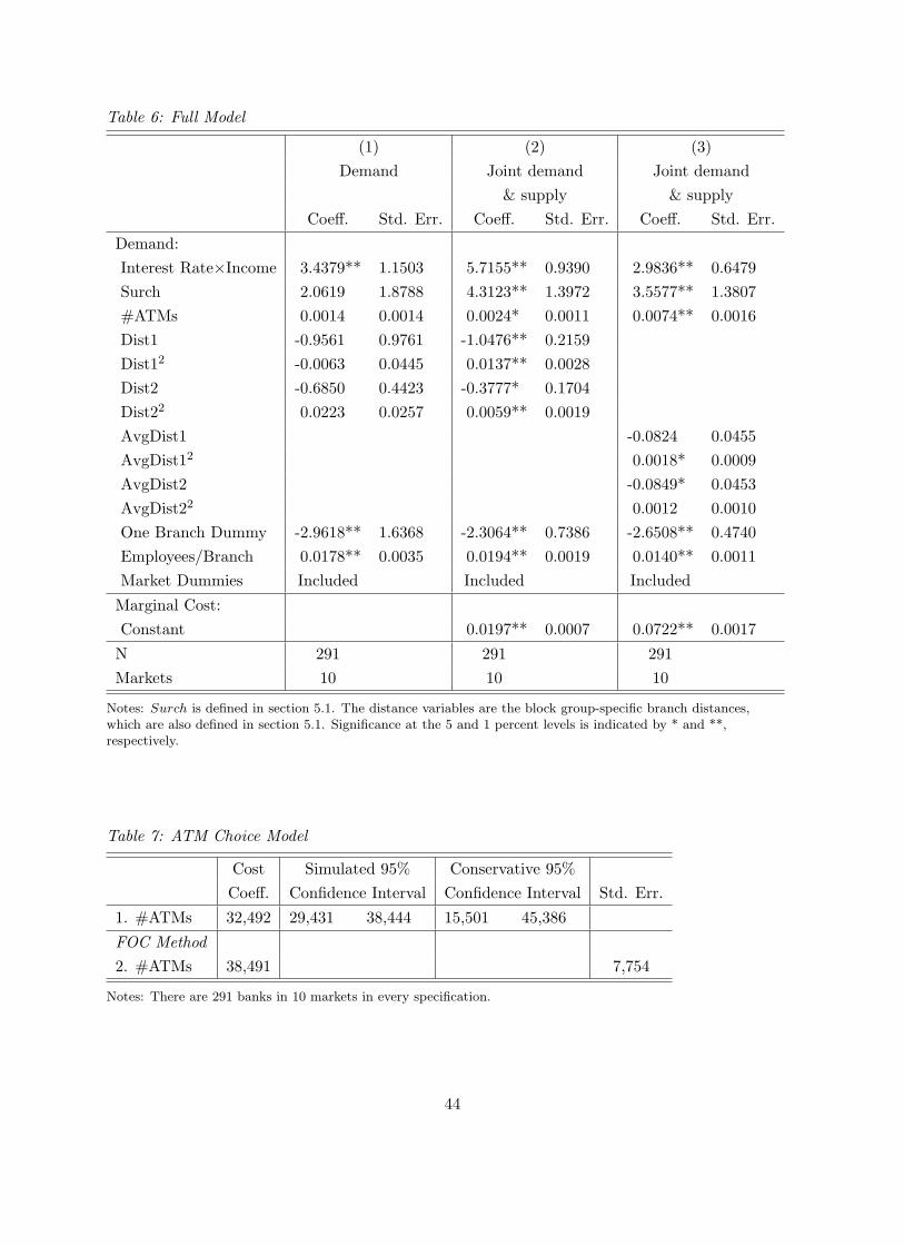
Table 6: Full Model

(1) (2) (3)Demand Joint demand Joint demand

& supply & supplyCoeff. Std. Err. Coeff. Std. Err. Coeff. Std. Err.

Demand:Interest Rate×Income 3.4379** 1.1503 5.7155** 0.9390 2.9836** 0.6479Surch 2.0619 1.8788 4.3123** 1.3972 3.5577** 1.3807#ATMs 0.0014 0.0014 0.0024* 0.0011 0.0074** 0.0016Dist1 -0.9561 0.9761 -1.0476** 0.2159Dist12 -0.0063 0.0445 0.0137** 0.0028Dist2 -0.6850 0.4423 -0.3777* 0.1704Dist22 0.0223 0.0257 0.0059** 0.0019AvgDist1 -0.0824 0.0455AvgDist12 0.0018* 0.0009AvgDist2 -0.0849* 0.0453AvgDist22 0.0012 0.0010One Branch Dummy -2.9618** 1.6368 -2.3064** 0.7386 -2.6508** 0.4740Employees/Branch 0.0178** 0.0035 0.0194** 0.0019 0.0140** 0.0011Market Dummies Included Included Included

Marginal Cost:Constant 0.0197** 0.0007 0.0722** 0.0017

N 291 291 291Markets 10 10 10

Notes: Surch is defined in section 5.1. The distance variables are the block group-specific branch distances,which are also defined in section 5.1. Significance at the 5 and 1 percent levels is indicated by * and **,respectively.

Table 7: ATM Choice Model

Cost Simulated 95% Conservative 95%Coeff. Confidence Interval Confidence Interval Std. Err.

1. #ATMs 32,492 29,431 38,444 15,501 45,386

FOC Method2. #ATMs 38,491 7,754

Notes: There are 291 banks in 10 markets in every specification.

44

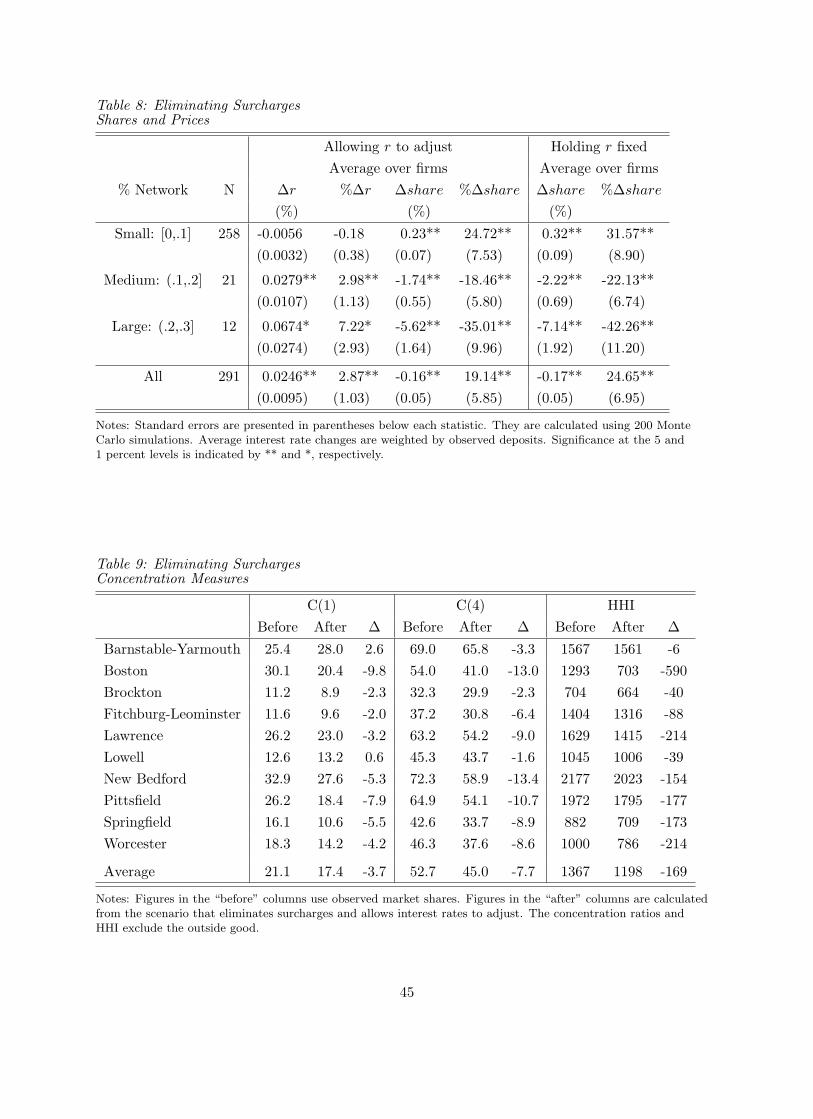
Table 8: Eliminating SurchargesShares and Prices

Allowing r to adjust Holding r fixedAverage over firms Average over firms

% Network N ∆r %∆r ∆share %∆share ∆share %∆share

(%) (%) (%)

Small: [0,.1] 258 -0.0056 -0.18 0.23** 24.72** 0.32** 31.57**(0.0032) (0.38) (0.07) (7.53) (0.09) (8.90)

Medium: (.1,.2] 21 0.0279** 2.98** -1.74** -18.46** -2.22** -22.13**(0.0107) (1.13) (0.55) (5.80) (0.69) (6.74)

Large: (.2,.3] 12 0.0674* 7.22* -5.62** -35.01** -7.14** -42.26**(0.0274) (2.93) (1.64) (9.96) (1.92) (11.20)

All 291 0.0246** 2.87** -0.16** 19.14** -0.17** 24.65**(0.0095) (1.03) (0.05) (5.85) (0.05) (6.95)

Notes: Standard errors are presented in parentheses below each statistic. They are calculated using 200 MonteCarlo simulations. Average interest rate changes are weighted by observed deposits. Significance at the 5 and1 percent levels is indicated by ** and *, respectively.

Table 9: Eliminating SurchargesConcentration Measures

C(1) C(4) HHIBefore After ∆ Before After ∆ Before After ∆

Barnstable-Yarmouth 25.4 28.0 2.6 69.0 65.8 -3.3 1567 1561 -6Boston 30.1 20.4 -9.8 54.0 41.0 -13.0 1293 703 -590Brockton 11.2 8.9 -2.3 32.3 29.9 -2.3 704 664 -40Fitchburg-Leominster 11.6 9.6 -2.0 37.2 30.8 -6.4 1404 1316 -88Lawrence 26.2 23.0 -3.2 63.2 54.2 -9.0 1629 1415 -214Lowell 12.6 13.2 0.6 45.3 43.7 -1.6 1045 1006 -39New Bedford 32.9 27.6 -5.3 72.3 58.9 -13.4 2177 2023 -154Pittsfield 26.2 18.4 -7.9 64.9 54.1 -10.7 1972 1795 -177Springfield 16.1 10.6 -5.5 42.6 33.7 -8.9 882 709 -173Worcester 18.3 14.2 -4.2 46.3 37.6 -8.6 1000 786 -214

Average 21.1 17.4 -3.7 52.7 45.0 -7.7 1367 1198 -169

Notes: Figures in the “before” columns use observed market shares. Figures in the “after” columns are calculatedfrom the scenario that eliminates surcharges and allows interest rates to adjust. The concentration ratios andHHI exclude the outside good.

45

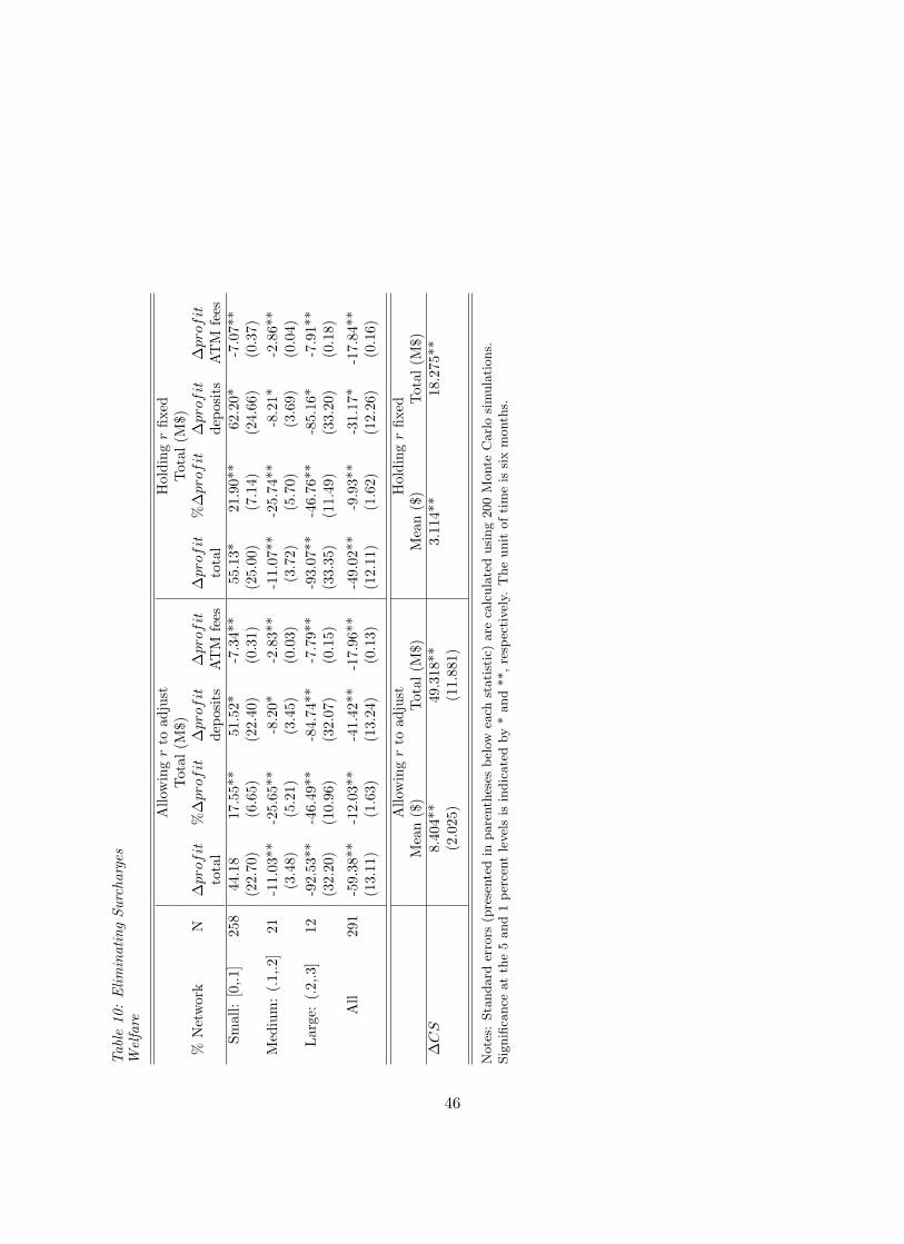
Tab

le10

:Elim

inat

ing

Surc

harg

esW

elfa

re

Allo

win

gr

toad

just

Hol

ding

rfix

edTot

al(M

$)Tot

al(M

$)%

Net

wor

kN

∆pro

fit

%∆

pro

fit

∆pro

fit

∆pro

fit

∆pro

fit

%∆

pro

fit

∆pro

fit

∆pro

fit

tota

lde

posi

tsA

TM

fees

tota

lde

posi

tsA

TM

fees

Smal

l:[0

,.1]

258

44.1

817

.55*

*51

.52*

-7.3

4**

55.1

3*21

.90*

*62

.20*

-7.0

7**

(22.

70)

(6.6

5)(2

2.40

)(0

.31)

(25.

00)

(7.1

4)(2

4.66

)(0

.37)

Med

ium

:(.

1,.2

]21

-11.

03**

-25.

65**

-8.2

0*-2

.83*

*-1

1.07

**-2

5.74

**-8

.21*

-2.8

6**

(3.4

8)(5

.21)

(3.4

5)(0

.03)

(3.7

2)(5

.70)

(3.6

9)(0

.04)

Lar

ge:

(.2,

.3]

12-9

2.53

**-4

6.49

**-8

4.74

**-7

.79*

*-9

3.07

**-4

6.76

**-8

5.16

*-7

.91*

*(3

2.20

)(1

0.96

)(3

2.07

)(0

.15)

(33.

35)

(11.

49)

(33.

20)

(0.1

8)

All

291

-59.

38**

-12.

03**

-41.

42**

-17.

96**

-49.

02**

-9.9

3**

-31.

17*

-17.

84**

(13.

11)

(1.6

3)(1

3.24

)(0

.13)

(12.

11)

(1.6

2)(1

2.26

)(0

.16)

Allo

win

gr

toad

just

Hol

ding

rfix

edM

ean

($)

Tot

al(M

$)M

ean

($)

Tot

al(M

$)∆

CS

8.40

4**

49.3

18**

3.11

4**

18.2

75**

(2.0

25)

(11.

881)

Note

s:Sta

ndard

erro

rs(p

rese

nte

din

pare

nth

eses

bel

owea

chst

ati

stic

)are

calc

ula

ted

usi

ng

200

Monte

Carl

osi

mula

tions.

Sig

nifi

cance

at

the

5and

1per

cent

level

sis

indic

ate

dby

*and

**,re

spec

tivel

y.T

he

unit

ofti

me

issi

xm

onth

s.

46

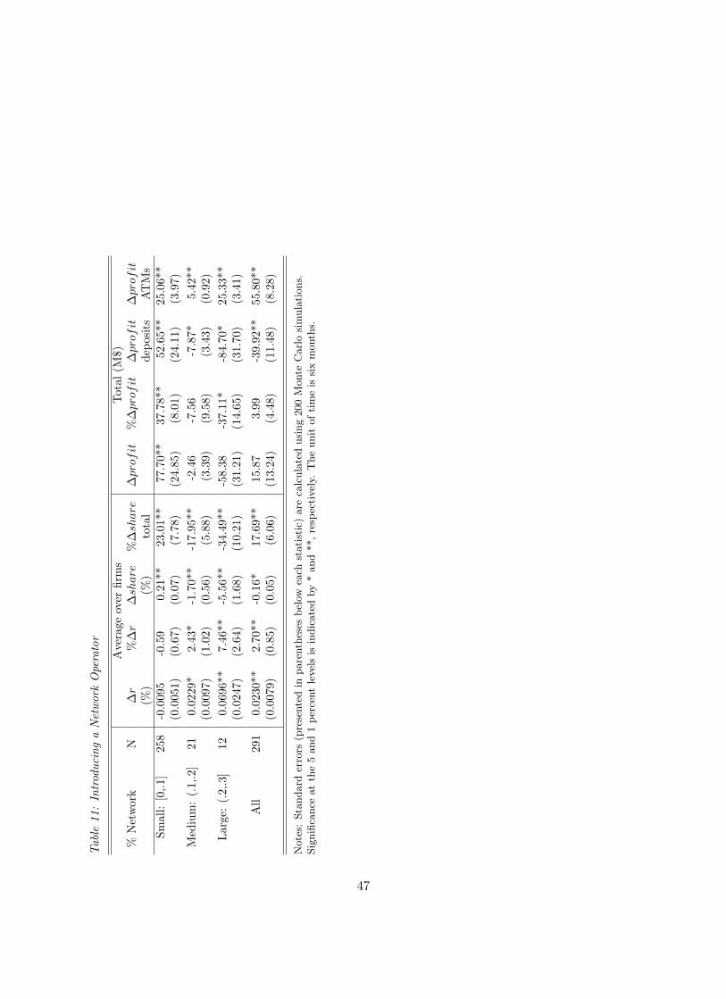
Tab

le11

:In

trod

ucin

ga

Net

wor

kO

pera

tor

Ave

rage

over

firm

sTot

al(M

$)%

Net

wor

kN

∆r

%∆

r∆

share

%∆

share

∆pro

fit

%∆

pro

fit

∆pro

fit

∆pro

fit

(%)

(%)

tota

lde

posi

tsA

TM

sSm

all:

[0,.1

]25

8-0

.009

5-0

.59

0.21

**23

.01*

*77

.70*

*37

.78*

*52

.65*

*25

.06*

*(0

.005

1)(0

.67)

(0.0

7)(7

.78)

(24.

85)

(8.0

1)(2

4.11

)(3

.97)

Med

ium

:(.

1,.2

]21

0.02

29*

2.43

*-1

.70*

*-1

7.95

**-2

.46

-7.5

6-7

.87*

5.42

**(0

.009

7)(1

.02)

(0.5

6)(5

.88)

(3.3

9)(9

.58)

(3.4

3)(0

.92)

Lar

ge:

(.2,

.3]

120.

0696

**7.

46**

-5.5

6**

-34.

49**

-58.

38-3

7.11

*-8

4.70

*25

.33*

*(0

.024

7)(2

.64)

(1.6

8)(1

0.21

)(3

1.21

)(1

4.65

)(3

1.70

)(3

.41)

All

291

0.02

30**

2.70

**-0

.16*

17.6

9**

15.8

73.

99-3

9.92

**55

.80*

*(0

.007

9)(0

.85)

(0.0

5)(6

.06)

(13.

24)

(4.4

8)(1

1.48

)(8

.28)

Note

s:Sta

ndard

erro

rs(p

rese

nte

din

pare

nth

eses

bel

owea

chst

ati

stic

)are

calc

ula

ted

usi

ng

200

Monte

Carl

osi

mula

tions.

Sig

nifi

cance

at

the

5and

1per

cent

level

sis

indic

ate

dby

*and

**,re

spec

tivel

y.T

he

unit

ofti

me

issi

xm

onth

s.

47

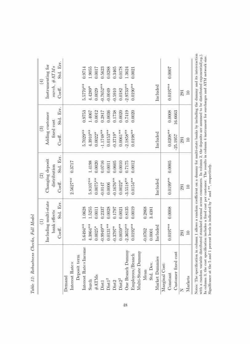
Tab

le12

:Rob

ustn

ess

Che

cks,

Full

Mod

el

(1)

(2)

(3)

(4)

Incl

udin

gm

ulti

-sta

teC

hang

ing

depo

sit

Add

ing

cust

omer

Inst

rum

enti

ngfo

rba

nkeff

ects

dist

ribu

tion

fixed

cost

surc

h,#

AT

Ms

Coe

ff.St

d.E

rr.

Coe

ff.St

d.E

rr.

Coe

ff.St

d.E

rr.

Coe

ff.St

d.E

rr.

Dem

and

Inte

rest

Rat

e×2.

5627

**0.

3717

Dep

osit

term

Inte

rest

Rat

e×In

com

e5.

6494

**1.

0628

5.70

29**

0.97

535.

5770

**0.

9714

Surc

h4.

3864

**1.

5255

5.81

07**

1.41

984.

3910

**1.

4067

4.42

89*

1.90

55#

AT

Ms

0.00

25*

0.00

110.

0075

**0.

0020

0.00

22*

0.00

120.

0029

0.00

17D

ist1

-0.9

949*

*0.

2337

-0.0

147

0.07

16-1

.174

8**

0.28

17-0

.765

2**

0.56

23D

ist1

20.

0131

**0.

0028

0.00

060.

0011

0.01

53**

0.00

36-0

.004

90.

0288

Dis

t2-0

.379

7*0.

1797

-0.1

676*

*0.

0605

-0.3

719*

0.17

38-0

.591

00.

3465

Dis

t22

0.00

59**

0.00

210.

0022

*0.

0010

0.00

61**

0.00

200.

0182

0.01

78O

neB

ranc

hD

umm

y-2

.365

2**

0.81

35-3

.551

8**

0.71

75-2

.185

8**

0.74

19-2

.973

3**

1.36

24E

mpl

oyee

s/B

ranc

h0.

0192

**0.

0019

0.01

54**

0.00

120.

0198

**0.

0020

0.01

90**

0.00

21M

ulti

-Sta

teD

umm

yM

ean

-0.0

762

0.28

68St

d.D

ev.

0.00

013.

4381

Mar

ket

Dum

mie

sIn

clud

edIn

clud

edIn

clud

edIn

clud

edM

argi

nalC

ost:

Con

stan

t0.

0197

**0.

0008

0.01

99**

0.00

050.

0208

**0.

0008

0.01

97**

0.00

07C

usto

mer

fixed

cost

-25.

1957

16.6

663

N29

129

129

129

1M

arke

ts10

1010

10

Note

s:T

he

spec

ifica

tion

inco

lum

n1

allow

sa

random

coeffi

cien

ton

adum

my

for

mult

i-st

ate

banks

by

incl

udin

gth

edum

my

and

its

inte

rera

ctio

nw

ith

ara

ndom

vari

able

dis

trib

ute

dst

andard

norm

alacr

oss

consu

mer

s.In

colu

mn

2,th

edep

osi

tsare

ass

um

edto

be

dis

trib

ute

dex

ponen

tial(

αy

i).

Inco

lum

n3,th

eco

stsp

ecifi

cati

on

incl

udes

afixed

cost

per

cust

om

er.

The

resu

lts

inco

lum

n4

inst

rum

ent

for

surc

harg

esand

AT

Mnet

work

size

.Sig

nifi

cance

at

the

5and

1per

cent

level

sis

indic

ate

dby

*and

**,re

spec

tivel

y.

48

Tab

le13

:Rob

ustn

ess

Che

cks,

Logi

tD

eman

dM

odel

(1)

(2)

(3)

(4)

Coe

ff.St

d.E

rr.

Coe

ff.St

d.E

rr.

Coe

ff.St

d.E

rr.

Coe

ff.St

d.E

rr.

Inte

rest

Rat

e21

7.37

7**

52.0

0320

5.07

7**

49.3

4921

4.65

5**

50.5

5721

4.24

8**

51.8

15Su

rch5

2.93

31.

544

#A

TM

s50.

053*

*0.

011

Sur

0.30

90.

325

SurS

UM

0.48

60.

368

Surn

on−

SU

M2.

257

1.17

7Su

rch

4.37

1**

1.47

8Su

rnoj

SU

M0.

358

0.32

1#

AT

Ms

0.00

8**

0.00

20.

008*

*0.

002

0.00

7**

0.00

2A

vgD

ist1

-0.0

94*

0.04

7-0

.087

0.04

8-0

.090

0.04

9-0

.093

0.04

8A

vgD

ist1

20.

002*

0.00

10.

002*

0.00

10.

002*

0.00

10.

002*

0.00

1A

vgD

ist2

-0.0

840.

047

-0.1

39**

0.04

5-0

.131

**0.

045

-0.0

91*

0.04

5A

vgD

ist2

20.

001

0.00

10.

002*

0.00

10.

002*

0.00

10.

001

0.00

1O

neB

ranc

hD

umm

y-2

.590

**0.

489

-3.1

91**

0.46

6-3

.102

**0.

481

-2.6

54**

0.48

6E

mpl

oyee

s/B

ranc

h0.

014*

*0.

001

0.01

4**

0.00

10.

014*

*0.

001

0.01

4**

0.00

1M

arke

tD

umm

ies

Incl

uded

Incl

uded

Incl

uded

Incl

uded

R2

0.81

30.

817

0.81

30.

819

N29

129

129

129

1M

arke

ts10

1010

10

Note

s:W

hit

ehet

erosk

edast

icity-c

onsi

sten

tst

andard

erro

rsare

use

d.

Sig

nifi

cance

at

the

5and

1per

cent

level

sis

indic

ate

dby

*and

**,

resp

ecti

vel

y.S

urc

h5

issu

rcharg

eco

sts

avoid

edw

ithin

afive-

mile

radiu

sand

#A

TM

s5is

num

ber

ofA

TM

sw

ithin

afive-

mile

radiu

s.

49

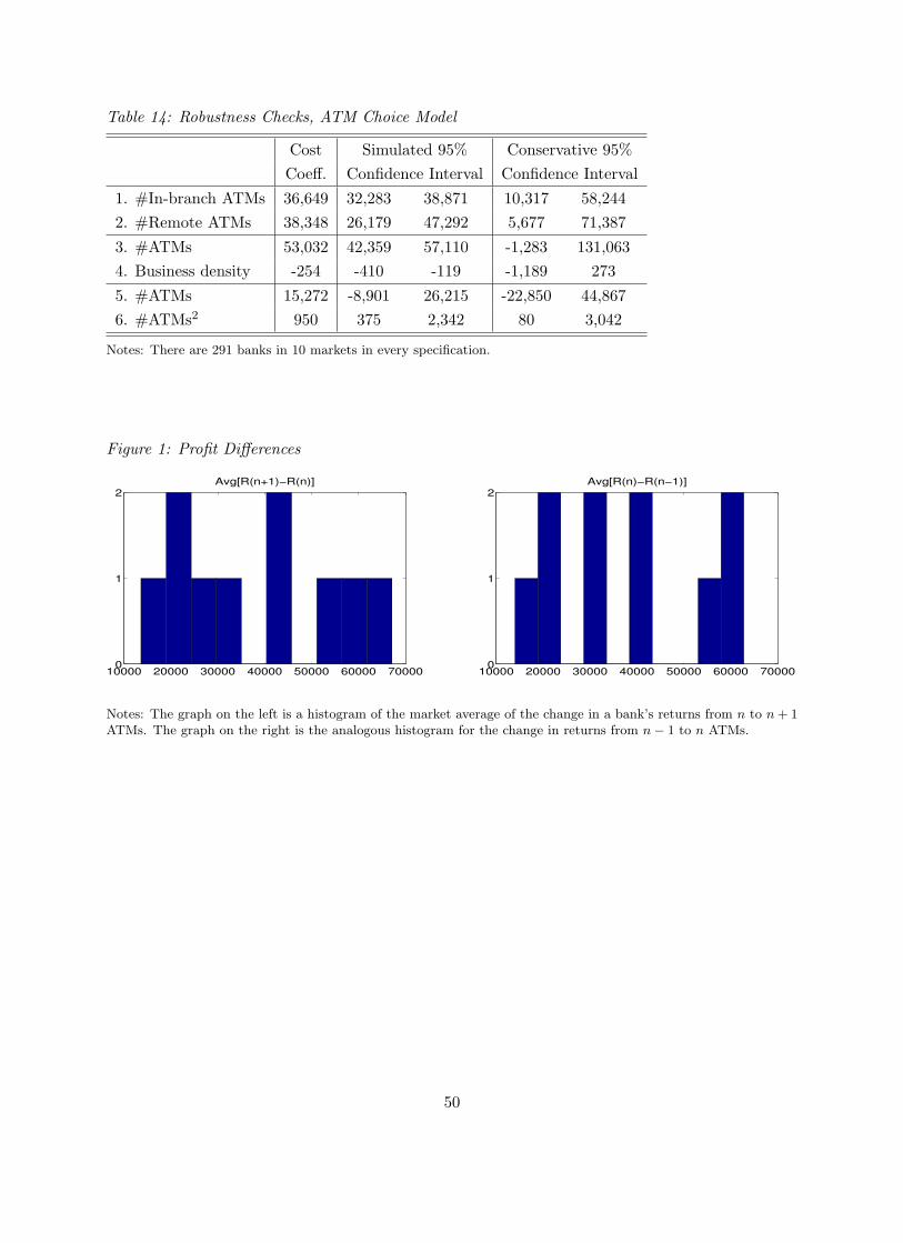
Table 14: Robustness Checks, ATM Choice Model

Cost Simulated 95% Conservative 95%Coeff. Confidence Interval Confidence Interval

1. #In-branch ATMs 36,649 32,283 38,871 10,317 58,2442. #Remote ATMs 38,348 26,179 47,292 5,677 71,387

3. #ATMs 53,032 42,359 57,110 -1,283 131,0634. Business density -254 -410 -119 -1,189 273

5. #ATMs 15,272 -8,901 26,215 -22,850 44,8676. #ATMs2 950 375 2,342 80 3,042

Notes: There are 291 banks in 10 markets in every specification.

Figure 1: Profit Differences

10000 20000 30000 40000 50000 60000 700000

1

2Avg[R(n+1)−R(n)]

10000 20000 30000 40000 50000 60000 700000

1

2Avg[R(n)−R(n−1)]

Notes: The graph on the left is a histogram of the market average of the change in a bank’s returns from n to n + 1ATMs. The graph on the right is the analogous histogram for the change in returns from n− 1 to n ATMs.

50