comparison of the musle model and two years of solid

water

Article

Comparison of the MUSLE Model and Two Years ofSolid Transport Measurement, in the Bouregreg Basin,and Impact on the Sedimentation in the SidiMohamed Ben Abdellah Reservoir, Morocco

Mohamed Abdellah Ezzaouini 1,2,* , Gil Mahé 3, Ilias Kacimi 1 and Abdelaziz Zerouali 2

1 Geoscience, Water and Environment Laboratory, Faculty of Sciences, Mohammed V University,Avenue Ibn Batouta, Rabat 10100, Morocco; [email protected]

2 Basin of the Bouregreg and Chaouia Agency, Benslimane BP 262, Morocco; [email protected] Laboratoire HydroSciences, Université Montpellier, IRD, 34090 Montpellier, France; [email protected]* Correspondence: [email protected]; Tel.: +212-661-110-897

Received: 18 May 2020; Accepted: 15 June 2020; Published: 1 July 2020��

Abstract: The evaluation and quantification of solids transport in Morocco often uses the UniversalSoil Loss Model (USLE) and the revised version RUSLE, which presents a calibration difficulty. In thisstudy, we apply the MUSLE model to predict solid transport, for the first time on a large river basinin the Kingdom, calibrated by two years of solid transport measurements on four main gaugingstations at the entrance of the Sidi Mohamed Ben Abdellah dam. The application of the MUSLE onthe basin demonstrated relatively small differences between the measured values and those expectedfor the calibrated version, these differences are, for the non-calibrated version, +5% and +102% for theyears 2016/2017 and 2017/2018 respectively, and between −33% and +34% for the calibrated version.Besides, the measured and modeled volumes that do not exceed 1.78 × 106 m3/year remain well belowthe dam’s siltation rate of 9.49 × 106 m3/year, which means that only 18% of the dam’s sedimentcomes from upstream. This seems very low because it is calculated from only two years. The mainhypothesis that we can formulate is that the sediments of the dam most probably comes from theerosion of its banks.

Keywords: modeling; MUSLE; erosion; solid transport; dam; Bouregreg; Morocco

1. Introduction

Erosion is a natural phenomenon that reduces the capacity of dam reservoirs around the world.The natural erosive process is aggravated by anthropogenic activities including pastoral activity [1],deforestation [2–4], and climate change [5] with the advent of periods of heavy rainfall and increasinglyfrequent dry periods. This phenomenon constitutes a major challenge for water resource managementat the scale of the Bouregreg basin [6,7] in northern Morocco.

The Sidi Mohamed Ben Abdellah (SMBA) dam, commissioned in 1974 and raised in 2007, isintended solely to supply drinking water to the coastal area between Rabat and Casablanca, whichrepresents nearly eight million inhabitants. It has a relatively low silting rate compared to other damsin the Kingdom [8].However, it has lost 132 Mm3 since its commissioning of which 58% of this volumewas lost before rising the dam height, with this loss constituting a very significant reduction in itsstorage capacity. Given the magnitude of this situation, the modeling of soil losses in the basin aims atachieving the following objectives:

• analyzing the biophysical environment;

Water 2020, 12, 1882; doi:10.3390/w12071882 www.mdpi.com/journal/water

http://www.mdpi.com/journal/water

http://www.mdpi.com

https://orcid.org/0000-0001-9140-1202

http://dx.doi.org/10.3390/w12071882

http://www.mdpi.com/journal/water

https://www.mdpi.com/2073-4441/12/7/1882?type=check_update&version=2

Water 2020, 12, 1882 2 of 27

• describing and evaluating the erosive processes affecting the Bouregreg Basin, and the solidtransport by the main tributaries to the SMBA dam;

• and identifying the priority areas contributing to siltation, in order to better guide spatialplanning actions.

Universal Soil Loss Equation (USLE) was first established in USA to model erosion in smallagricultural catchment [9]. It is based on several parameters linked to climate, soil cover and properties,topography, and human activities. This equation has been modified and adapted several times.The MUSLE model includes the use of water flow rates [10]. Despite the difficulties encounteredin calibrating and adapting the Universal Land Loss Model (USLE) to conditions in Morocco [11],most studies on watershed management in Morocco [12–15] and bordering Mediterranean regions, inparticular in Algeria and Tunisia [15–17], continue to use USLE, and the revised version RUSLE [18–21],or an event normalized plot soil loss estimated by a modified USLE model—USLE-MM—as in Italy [22],most often for small basins of much less than 5000 km2. As USLE [23] and RUSLE [24] were developedfor the rough assessment of annual land loss at the scale of small plots, their application to large areasleads to rather large errors [25,26]. However, their accuracy increases when coupled with hydrologicalmodels [27]. To overcome the difficulties in assessing the accuracy of using a simple erosion equationlike USLE, Alewell et al. [28] recommend to strengthen and extend measurement and monitoringprograms to build up validation data sets.

Thus, Williams [10] developed a modified version of the USLE (MUSLE) that takes into accountthe flow load at the outlet by taking into account the biophysical characteristics of the watershed.This model has already been applied to micro-watersheds [29,30] and gave very reliable resultscompared to measurements. Indeed, in the Sidi Sbaa basin in Morocco, the deviation of the resultscompared to the MUSLE model was −4% by underestimating the solid inputs [31]. Samaras andKoutitas et al. [32] use MUSLE with SWAT to simulate the potential impact of land cover change onsediment yields to the sea in Greece, but with no observed validation data; while other authors likeFang [33] use the WaTEM/SEDEM model, which includes the RUSLE formula, to estimate erosion,but always without observations to compare. Only a few studies compare the erosion rates with thethree USLE formulas. In Maghreb, only one study by Djoukbala et al. [34] compared them on the smallbasin of 384 km2 in the north of Algeria, with erosion rates quite similar between the three methods,but they were slightly superior in the case MUSLE. Unfortunately, they could not compare their resultswith observation data, which does not allow an assessment of the validity of the erosion rates producedin regard to real natural processes.

2. Materials and Methods

2.1. Study Area

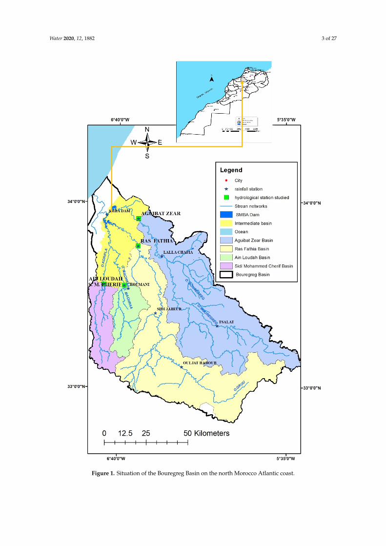
The Bouregreg Basin, located in central western Morocco, covers a total area of approximately10,130 km2 at its mouth in the north of the city of Rabat (Figure 1). The main rivers of the basin are theBouregreg, the Grou, and the Korifla and its tributary, the Machraa.

Water 2020, 12, 1882 3 of 27

Water 2020, 12, x FOR PEER REVIEW 3 of 26

Figure 1. Situation of the Bouregreg Basin on the north Morocco Atlantic coast.

Water 2020, 12, 1882 4 of 27

The climate in the study area is Mediterranean with oceanic influence, with an average annualrainfall over the basin varying from 450 mm in Rabat in the north-west, to nearly 750 mm in themountainous area in the south-east.

Rain events generate water volume of 680 × 106 m3/year, i.e., an annual mean of 22 m3/s. It isregulated by the capacity of the SMBA dam, located downstream of the confluence between theBouregreg, Korifla/Machraa, and Grou rivers. Table 1 summarizes the characteristics of the SMBA dam.

Table 1. Sidi Mohamed Ben Abdellah (SMBA)dam data.

WatershedArea(km2)

Initial DamCapacity (106 m3)

Inter-AnnualWater Resources

(106 m3)Opening Date

Number ofBathymetric

Measurements

SMBA at itsconstruction

9800508.6

6801974 5

SMBA afterraising its dike 974.0 2007 3

2.2. Basic Data

2.2.1. Discharges Measurements

The hydrometric network of the Bouregreg basin upstream of the SMBA dam is composed of threemajor tributaries: Bouregreg, Grou, and Korifla (including its tributary the Machraa). Four hydrologicalstations located on these tributaries at the entrance of the dam’s reservoir were chosen to carry outthe measurements of solid transport. These hydrological stations control a basin of about 8521 km2,i.e., 87% of the catchment area of the SMBA dam. They also have human and material means toensure the measurement of flows, rainfall, and the concentration of suspended solids. Table 2 gives thecharacteristics of the four hydrological stations.

Table 2. Characteristics of the four hydrological stations studied.

HydrologicalStation

Name ofRiver

Date ofCommissioning

AveragingPeriod

N◦IREABHBC

Code

WatershedArea(km2)

Lambert Coordinates

X Y Z

Aguibat Zear Bouregreg 1975 1975/2018 3118/13 3681 394.500 368.150 90Ras Fathia Grou 1975 1975/2018 989/20 3485 394.250 351.800 100

Ain Loudah Korifla 1971 1971/2018 2673/20 699 373.750 329.150 175Sidi

MohamedCherif

Machraa 1971 1971/2018 2674/21 656 385.850 328.200 270

Figure 2 shows that the two years, 2016/2017 and 2017/2018, are dry years which did not recordsignificant water inflows.

Examination of the historical measurement data from the four observation stations shows that80% of the inflows to the dam are recorded between October and May (Figure 3). The Bouregreg andGrou rivers contribute more than 90% of the inflows generated in the basin.

Table 3 shows the maximum flows, volumes, and number of flood events recorded during the2016/2017 and 2017/2018 hydrological years at the four hydrological stations studied. The number ofrecorded events is between six and seventeen, depending on the observation station and the year.

Water 2020, 12, 1882 5 of 27


Figure 2 shows that the two years, 2016/2017 and 2017/2018, are dry years which did not record significant water inflows.

Figure 2. Annual discharges at the 4 hydrological stations studied.

Examination of the historical measurement data from the four observation stations shows that 80% of the inflows to the dam are recorded between October and May (Figure 3). The Bouregreg and Grou rivers contribute more than 90% of the inflows generated in the basin.

Figure 3. Mean monthly discharges at the hydrological stations studied.

Table 3 shows the maximum flows, volumes, and number of flood events recorded during the 2016/2017 and 2017/2018 hydrological years at the four hydrological stations studied. The number of recorded events is between six and seventeen, depending on the observation station and the year.

0

5

10

15

20

25

30

35

40

197

2/73

197

4/75

197

6/77

197

8/79

198

0/81

198

2/83

198

4/85

198

6/87

198

8/89

199

0/91

199

2/93

199

4/95

199

6/97

199

8/99

200

0/01

200

2/03

200

4/05

200

6/07

200

8/09

201

0/11

201

2/13

201

4/15

201

6/17

201

8/19

Run

-off

(m3 /s

)

Year

Aguibat Zear Ras Fathia Ain Loudah Sidi Mohamed Cherif

0

5

10

15

20

25

Run

-off

(m3 /s

)

MonthAguibat Zear Ras Fathia Ain Loudah Sidi Mohammed Cherif



Figure 2 shows that the two years, 2016/2017 and 2017/2018, are dry years which did not record significant water inflows.


Examination of the historical measurement data from the four observation stations shows that 80% of the inflows to the dam are recorded between October and May (Figure 3). The Bouregreg and Grou rivers contribute more than 90% of the inflows generated in the basin.


Table 3 shows the maximum flows, volumes, and number of flood events recorded during the 2016/2017 and 2017/2018 hydrological years at the four hydrological stations studied. The number of recorded events is between six and seventeen, depending on the observation station and the year.

0

5

10

15

20

25

30

35

40

197

2/73

197

4/75

197

6/77

197

8/79

198

0/81

198

2/83

198

4/85

198

6/87

198

8/89

199

0/91

199

2/93

199

4/95

199

6/97

199

8/99

200

0/01

200

2/03

200

4/05

200

6/07

200

8/09

201

0/11

201

2/13

201

4/15

201

6/17

201

8/19

Run

-off

(m3 /s

)

Year

Aguibat Zear Ras Fathia Ain Loudah Sidi Mohamed Cherif

0

5

10

15

20

25

Run

-off

(m3 /s

)

MonthAguibat Zear Ras Fathia Ain Loudah Sidi Mohammed Cherif


Table 3. Flood events for the four hydrological stations studied.

HydrologicalStation

HydrologicalYear

MaximumDischarge

Recorded Per Year(m3/s)

Date of Flood Event Volume(106 m3)

Number ofFlood Events

Aguibat Zear 2016/2017 263.4 24/02/2017 at 23h00 52 132017/2018 265.9 07/03/2018 at 14h00 77 14

Ras Fathia2016/2017 256.4 25/02/2017 at 07h30 33 112017/2018 423.8 07/03/2018 at 09h00 59 10

Ain Loudah2016/2017 24.5 13/10/2016 at 11h00 0.7 102017/2018 198.7 24/04/2018 at 23h00 7.6 17

Sidi MohamedCherif

2016/2017 62.6 13/10/2016 at 07h00 1.8 62017/2018 48.0 11/12/2017 at 17h00 1.28 6

2.2.2. Concentration of Suspended Solids (CSS)

Observers at the four hydrological stations studied, who are contracted by the Hydraulic Basin ofthe Bouregreg and Chaouia Agency (ABHBC), carry out daily sampling during low-flow periods andhourly sampling during periods of flooding. At each instantaneous sampling, the date, time, and scale

Water 2020, 12, 1882 6 of 27

rating are noted on the specimen bottles catalogued. The samples are then analyzed in the laboratoryand filtered under a vacuum using filtering membranes (0.45µm). The available data for measuring theconcentration of suspended solids cover two hydrological years, 2016/2017 and 2017/2018. The numberof measurement samples is presented in Table 4.

Table 4. Number of concentration of suspended solids (CSS)samples and floods events per station.

Name of HydrologicalStation River Watershed

Area (km2) 2016/2017 and 2016/2018

Number of CSSSamples

Number of FloodEvents

AguibatZear Bouregreg 3681 727 27Ras Fathia Grou 3485 636 21

Ain Loudah Korifla 699 233 27Sidi Mohamed Cherif Machraa 656 789 12

2.2.3. Bathymetric Data

In order to draw up an inventory of the silting of the SMBA dam reservoir, the bathymetricsurveys carried out by the Moroccan Directorate of Water Research and Planning were collected andanalyzed. A total of seven bathymetric surveys were collected, the oldest dating back to 1974, whilethe most recent were carried out in 2013. Analysis of the bathymetric data shows that the siltingup of the SMBA dam reservoir was of the order of 2.65 × 106 m3/year, i.e., a specific degradation of270.4 m3/km2/year before raising. After raising, the silting increased to 9.49 × 106 m3/year, i.e. a specificdegradation of 968.37 m3/km2/year, which increased the silting rate by 400% [4]. However, the data issubject to doubt for values in the early 2000s [35].The difference between the beginning and the end ofthe chronicle is of reliable quality. Therefore, the total silting of the SMBA dam reached 132 ×106 m3,i.e., an average silting rate of 3.7 × 106 m3/year since its commissioning. Subsequently, the dam hasexceeded its dead unit, which is sized for 100 × 106 m3 and has lost 32 × 106 m3of its useful reservesince its commissioning. Table 5 summarizes the silting status of the dam.

Table 5. Summary of SMBA dam siltation calculation results since its impoundment.

Name of theDam

Initial DamCapacity(106 m3)

TotalSiltation(106 m3)

Numberof Years

Rate ofSiltation(106 m3)

Dead-unitVolume at

DamBuilding(106m3)

LostVolume

(%)

CurrentCapacity(106 m3)

SMBA beforeraising 508.60 76.88 29 2.65

100.0015 431.72

SMBA afterraising 974.79 55.28 6 9.49 6 919.51

The silting of the dam reservoir represents a real threat to the sustainability of the mobilizationof surface water resources in the Bouregreg basin to satisfy required needs. The regulation of theSMBA dam, prior to its raising, was done on a seasonal basis (capacity lower than the annual inflow).In other words, the dam had to discharge the surplus inflows most often from flood spillway orbottom discharge. This technique of management favored the elimination of solid deposits and thusa reduction in the siltation rate of the dam. After the dam was raised and consequently the watercapacity of the reservoir increased, the SMBA dam moved to multi-year regulation (capacity greaterthan annual inflows). By using the restitution devices of the dam, this method of regulation favorsstorage to the detriment of evacuation, which accentuates the silting rate. Figure 4 illustrates theevolution over time of the normal capacity of the SMBA dam.

Water 2020, 12, 1882 7 of 27


Name of the Dam

Initial Dam

Capacity (106 m3)

Total Siltation (106 m3)

Number of Years

Rate of Siltation (106 m3)

Dead-unit Volume at Dam

Building (106m3)

Lost Volume

(%)

Current Capacity (106 m3)

SMBA before raising

508.60 76.88 29 2.65

100.00

15 431.72

SMBA after

raising 974.79 55.28 6 9.49 6 919.51

The silting of the dam reservoir represents a real threat to the sustainability of the mobilization of surface water resources in the Bouregreg basin to satisfy required needs. The regulation of the SMBA dam, prior to its raising, was done on a seasonal basis (capacity lower than the annual inflow). In other words, the dam had to discharge the surplus inflows most often from flood spillway or bottom discharge. This technique of management favored the elimination of solid deposits and thus a reduction in the siltation rate of the dam. After the dam was raised and consequently the water capacity of the reservoir increased, the SMBA dam moved to multi-year regulation (capacity greater than annual inflows). By using the restitution devices of the dam, this method of regulation favors storage to the detriment of evacuation, which accentuates the silting rate. Figure 4 illustrates the evolution over time of the normal capacity of the SMBA dam.

Figure 4. Evolution of the normal capacity of the SMBA dam reservoir, in millions of m3.

2.3. Methods

2.3.1. Model Selection

In this study we apply the Williams [10] model based on the Modified Universal Soil Loss Equation (MUSLE), integrated in the ArcGIS Geographic Information System for the determination of the soil loss potential at the level of the Bouregreg watershed to the four hydrological stations located immediately upstream of the SMBA dam, as previously done by Khali Issa et al.[37] in another region of Morocco in the North of the country, over a very small basin of 38 km².

This model evaluates the average annual rate of erosion at the outlet of the basin. It uses hydrological parameters, measured at the four hydrological stations, taking into account biophysical characteristics. Thus, the model equation is as follows: = ( × ) × × × , (1)

508.60 486.33 457.94 425.12 431.72

974.79 937.03 919.51

0

200

400

600

800

1000

1200

1974 1985 1995 2000 2003 2007 2009 2013

Vol

ume

(106

m3 )

Year

Figure 4. Evolution of the normal capacity of the SMBA dam reservoir, in millions of m3.

2.3. Methods

2.3.1. Model Selection

In this study we apply the Williams [10] model based on the Modified Universal Soil Loss Equation(MUSLE), integrated in the ArcGIS Geographic Information System for the determination of the soil losspotential at the level of the Bouregreg watershed to the four hydrological stations located immediatelyupstream of the SMBA dam, as previously done by Khali Issa et al. [36] in another region of Moroccoin the North of the country, over a very small basin of 38 km2.

This model evaluates the average annual rate of erosion at the outlet of the basin. It useshydrological parameters, measured at the four hydrological stations, taking into account biophysicalcharacteristics. Thus, the model equation is as follows:

A = a(Qmax ×Vt)bK × LS×C× P, (1)

where A: amount of sediment produced at the outlet in tons, a and b: in this study, we used thescale factor values of the Sidi Sbaa micro-basin [30] (a = 11.8 and b = 0.56), Qmax: maximum flowrate in m3/s, Vt: total volume of runoff water in m3, K: average soil erodibility (mg MJ-1mm-1), LS:average topographic factor, C: average vegetation cover factor, P: average cultural practices andamenities factor.

2.3.2. Methods Selection

We adopted the suite of methods and operations explained in the flowchart (Figure 5) below toassess siltation rates at hydrological stations upstream of the SMBA dam [37].

Water 2020, 12, 1882 8 of 27


where : amount of sediment produced at the outlet in tons, a and b: in this study, we used the scale factor values of the Sidi Sbaa micro-basin [30](a=11.8 and b = 0.56), : maximum flow rate in m3/s, : total volume of runoff water in m3, : average soil erodibility (mg MJ-1mm-1), : average topographic factor, : average vegetation cover factor, : average cultural practices and amenities factor.

2.3.2. Methods Selection

We adopted the suite of methods and operations explained in the flowchart (Figure 5) below to assess siltation rates at hydrological stations upstream of the SMBA dam [38].

Figure 5. Methodology adopted for the assessment of erosion in the Bouregreg basin.

3. Results

3.1.Rainfall and Hydrometric Analysis

Solid transports are calculated at the four hydrological stations concerned in the hydrological years 2016/2017 and 2017/2018. These two years were respectively dry and wet in terms of rainfall. The average rainfall recorded at all the rainfall stations in the basin reached 354 mm in 2016/2017 and 496 mm in 2017/2018. Thus, the rainfall differences recorded in relation to the arithmetic mean of the data from the rainfall stations located in the Bouregreg basin varied respectively by −10% and +26% since the commissioning dates of the stations, based on data available to study from the ABHBC.

Table 6 summarizes the rainfall variations recorded in relation to the average rainfall of the stations in the Bouregreg basin.

Figure 5. Methodology adopted for the assessment of erosion in the Bouregreg basin.

3. Results

3.1. Rainfall and Hydrometric Analysis

Solid transports are calculated at the four hydrological stations concerned in the hydrologicalyears 2016/2017 and 2017/2018. These two years were respectively dry and wet in terms of rainfall.The average rainfall recorded at all the rainfall stations in the basin reached 354 mm in 2016/2017 and496 mm in 2017/2018. Thus, the rainfall differences recorded in relation to the arithmetic mean of thedata from the rainfall stations located in the Bouregreg basin varied respectively by −10% and +26%since the commissioning dates of the stations, based on data available to study from the ABHBC.

Table 6 summarizes the rainfall variations recorded in relation to the average rainfall of the stationsin the Bouregreg basin.

Table 6. Rainfall for the 2016/2017 and 2017/2018 water years.

Rain GaugeStation Basin Cumulative Rainfall

(mm)Averaging

Period

MeanYear(mm)

Deviationfrom the Mean

(%)2016/2017 2017/2018 2016/2017 2017/2018

LallaChafia Bouregreg 409 569 1972/2019 486 −16 17AguibatZear Bouregreg 482 578 1975/2019 429 12 35Sidi Jabeur Grou 260 432 1971/2019 317 −18 36

Tsalat Bouregreg 454 622 1977/2019 469 −3 33Roumani Machraa 261 431 1933/2019 342 −24 26

Ras Fathia Grou 290 505 1975/2019 387 −25 30S. M Cherif Machraa 290 495 1971/2019 367 −21 35

Barrage SMBA Bouregreg 518 479 1984/2019 469 10 2OuljatHaboub Grou 321 350 1972/2019 311 3 12Ain Loudah Krofla 258 498 1971/2019 347 −26 43

Total 354 496 392 −10 26

Water 2020, 12, 1882 9 of 27

With the exception of the Korifla sub-basin at the right of the Ain Loudah station which recordeda surplus of nearly 24% during 2017/2018, the contributions were in deficit on the rest of the sub-basinsduring the two hydrological years with more pronounced deficits during the dry year 2016/2017.Table 7 summarizes the inflows recorded at the four stations of the study.

Table 7. Water supplies to the four hydrological stations studied.

HydrologicalStation River Water Supply (Mm3)

Deviationfrom the Mean (%)

2016/2017 2017/2018 AveragingPeriod

AnnualAverage

(mm)2016/2017 2017/2018

AguibatZear Bouregreg 122.2 221.5 1975/2019 227.6 −46 −3Ras Fathia Grou 95.0 162.8 1975/2019 194.2 −51 −16

Ain Loudah Korifla 13.3 23.5 1971/2019 18.9 −29 +24Sidi

MohammedCherif

Machraa 3.7 12.9 1971/2019 16.7 −77 −23

3.2. Analysis of the Biophysical Environment

The analysis of the biophysical environment consists of determining the average factors used bythe model for each sub-basin. These factors, that affect soil erosion, are: soil type, topography, land useand cropping practices, and erosion control facilities [38].

3.2.1. Soil Erodibility Factor (K)

Erodibility is defined as the degree to which soils are resistant to erosion. The factors that have amajor influence on the response of soils to erosion, namely the detachment and transport of particlesby rain and runoff, are texture, structure, organic matter, and permeability. The methodology forestimating RUSLE K has been applied, and is written as follows [39]:

K =[2.1× 10−4(12−MO)M1.14 + 3.25(S− 2) + 2.5(P− 3)

]/10, (2)

with K: soil erodibility expressed in t.ha.h/ha.MJ.mm (tonne. hectare. hour/hectare. mega joule.millimeter); MO: percentage of organic matter; M: textural term % fine sand + % silt; S: structure classcode 1 to 4, with 1 fragmented structure and 4 coarse structure, soil structure affects both landslidesusceptibility and infiltration, the profiles described on the Bouregreg have a subangular polyhedralstructure and fall under class (3); and P: the permeability code (1 to 6), its value can be inferredindirectly from the organic matter content by calculating the infiltration given by the Equation [40]:

Y = 3.53×X + 2.08, (3)

with: Y = infiltration in cm/h, X = organic matter in %.Thereafter, the soil erodibility factor K will be calculated using the Harmonized World Soil

Database (HWSD), developed by the Food and Agriculture Organization of the United Nations (FAO)(http://www.fao.org/soils-portal/fr/). This database gives the distribution of silt, sand, and clay soilcompositions by soil type [41].

Soil is composed of organic and mineral matter. Its texture is determined by the size of the soilparticles and their respective quantities. There are three categories of particles that determine soiltexture: sand, silt, and clay. They are distinguished by particle diameter: sand 0.05 mm to 2 mm, silt0.002 mm to 0.05 mm, clay 0.002 mm and less. The modified illustrated triangular graph [42] was usedto determine soil texture classification.Soil texture is classified according to the percentage of silt, sand,and clay.

http://www.fao.org/soils-portal/fr/

Water 2020, 12, 1882 10 of 27

Once the textures have been determined, it is possible to establish the correspondence betweenthe standard texture and the K-factor [43]. These values are given in tons/ha and ton/acre (US system).Although this methodology provides an approximation in the calculation of the K-factor, it has theadvantage of lending itself to the constraints imposed by the study area. The rate of organic matterat the level of each watershed for each texture value is calculated by converting organic carbon intoorganic matter. The conversion factor of 1.724 is commonly used to convert the organic carbon contentof a soil sample to organic matter. The conversion factor is old and has survived the test of time andmodern analytical methods. According to authors [44], this conventional factor is attributed to the 19thcentury authors Van Bemmelen [45], Wolff [46], or even Sprengel [47]. It is based on well-establishedand very old studies showing that soil organic matter contains 58% carbon. Since the C/MO ratiowould be equal to 0.58, the MO/C ratio would be equal to 1.724.

Thus, the calculation of the organic matter is carried out by the following formula, which uses thevalue 1.724 and is widely used in Morocco:

MO = CO× 1.724, (4)

the average erodibility factor K per basin is calculated by the formula:

Kaverage =

∑(K× number)∑

number, (5)

with K: K-factor per value, number: counting of pixels with the same K-value in the Arcmapallocation table.

The results of the calculation of the average K-factor for each watershed are in Table 8.

Table 8. Average erodibility factor for each watershed.

Name Watershed Erodibility Factor Kaverage

Bouregreg 0.352Grou 0.350

Ain Loudah 0.348Sidi Mohamed Cherif 0.348

The Kmoy factor used is 0.35. This value corresponds to the silt, with the latter being a sedimentaryformation whose grains are of intermediate size between clays and sands. The loss of silt leads toa decrease in the water retention capacity of the soil. The result is an increased erodibility and anincreased risk of erosion. Because silt is often suspended in water, it is easily transported by floods andcan contribute to the siltation of dam reservoirs. Figure 6 shows the distribution of the K factor over theBouregreg basin for the four hydrological stations located immediately upstream of the SMBA dam.

Water 2020, 12, 1882 11 of 27


factor over the Bouregreg basin for the four hydrological stations located immediately upstream of the SMBA dam.

Figure 6. K-factor of the Bouregreg basin at the four hydrological stations.

3.2.2. Topographic Factor (LS)

The topographic factor LS is an essential parameter of the model. It expresses the result of erosion due to the combined effect of the degree of slope and its length. Most recent studies for the determination of the soil loss potential at the watershed level by the MUSLE model utilize the equation established by Wischmeier and Smith [23,9], which is expressed as: = ( ʎ. ) × 65.4 sin² β + 4.56 sin β + 0.0654, (6)

with:ʎ: length of the slope in m, : slope in degrees, m=0.5 if β ≥ 5%, m= 0.3 if 1<β < 5%, m= 0.2 if β≤1. First, the slope map was established by the spatial analyst tool of the ArcGis software using a 90

m resolution DTM. Then, the LS map (Figure 7) by basin was generated using the Wishmeierand Smith formula [23,9]. The mean slopes and mean LS values are given in Table 9.

Table 9. Mean slope and mean topographic factor (LS).

Mean Slope

(%) Mean Topographic Factor (Ls)

Bouregreg à Lala Chafia 16.6 0.48 Grou à Ras Fathia 14.6 0.49

Korifla à Ain Loudah 9.8 0.27 Machraa à Sidi Mohamed Cherif 12.2 0.58



The topographic factor LS is an essential parameter of the model. It expresses the result oferosion due to the combined effect of the degree of slope and its length. Most recent studies for thedetermination of the soil loss potential at the watershed level by the MUSLE model utilize the equationestablished by Wischmeier and Smith [9,23], which is expressed as:

LS =(





The topographic factor LS is an essential parameter of the model. It expresses the result of erosion due to the combined effect of the degree of slope and its length. Most recent studies for the determination of the soil loss potential at the watershed level by the MUSLE model utilize the equation established by Wischmeier and Smith [23,9], which is expressed as: 𝐿𝑆 = ( ʎ. ) × 65.4 sin² β + 4.56 sin β + 0.0654, (6)

with:ʎ: length of the slope in m, 𝛃: slope in degrees, m=0.5 if β ≥ 5%, m= 0.3 if 1<β < 5%, m= 0.2 if β≤1. First, the slope map was established by the spatial analyst tool of the ArcGis software using a 90



Mean Slope




22.13

)m× 65.4 sin2 β+ 4.56 sinβ+ 0.0654, (6)

with:





The topographic factor LS is an essential parameter of the model. It expresses the result of erosion due to the combined effect of the degree of slope and its length. Most recent studies for the determination of the soil loss potential at the watershed level by the MUSLE model utilize the equation established by Wischmeier and Smith [23,9], which is expressed as: 𝐿𝑆 = ( ʎ. ) × 65.4 sin² β + 4.56 sin β + 0.0654, (6)

with:ʎ: length of the slope in m, 𝛃: slope in degrees, m=0.5 if β ≥ 5%, m= 0.3 if 1<β < 5%, m= 0.2 if β≤1. First, the slope map was established by the spatial analyst tool of the ArcGis software using a 90



Mean Slope




: length of the slope in m, β: slope in degrees, m = 0.5 if β ≥ 5%, m = 0.3 if 1 < β < 5%, m = 0.2 ifβ ≤ 1.

First, the slope map was established by the spatial analyst tool of the ArcGis software using a90 m resolution DTM. Then, the LS map (Figure 7) by basin was generated using the WishmeierandSmith formula [9,23]. The mean slopes and mean LS values are given in Table 9.


Mean Slope(%) Mean Topographic Factor (Ls)

Bouregreg à Lala Chafia 16.6 0.48Grou à Ras Fathia 14.6 0.49

Korifla à Ain Loudah 9.8 0.27Machraa à Sidi Mohamed Cherif 12.2 0.58

Water 2020, 12, 1882 12 of 27Water 2020, 12, x FOR PEER REVIEW 12 of 26

Figure 7. LS factor of the Bouregreg basin at the four hydrological stations.

3.2.3. Land Cover Factor (C)

The soil protection factor (C) indicates the degree of soil protection by vegetation cover. This factor has undergone several changes since the establishment of the universal soil loss equation. The vegetation cover is—after topography—the second most important factor controlling the risk of soil erosion. The value of C depends mainly on the percentage of vegetation cover and the growth phase. The Cfactor map for the Bouregreg catchment area was derived from the land use maps. These were determined from the use of remote sensing data and field observations [49]. The land cover map was extracted from SPOT satellite images at 20 m resolution combined with recent Landsat ETM+ images (2011/2012) using the supervised classification method [42]. Another approach could be to derive the C factor from NDVI maps as practiced on the Wadi Mina in Algeria by Toumi et al.[16]

The distribution of surfaces according to the nature of the vegetation cover is carried out by the ArcGis tool, which subdivides the catchment area into several polygons. Each polygon corresponds to a specific type of vegetation cover. Each vegetation cover corresponds to a factor given by Wischmeir and Smith according to the theme [50]. A color is assigned to each polygon that represents a land cover type. For the calculation of the Cfactor, an independent calculation is required for each sub-basin. Indeed, the sensitivity to erosion of the different classes is determined from the main land use themes, i.e., forest formations, rangelands, agricultural land, arboriculture, water, and bare soil, whose values vary between 0 and 1. The calculation of the average vegetation cover factor depends on the factor given for each land use and surface area by the following formula:

Figure 7. LS factor of the Bouregreg basin at the four hydrological stations.

3.2.3. Land Cover Factor (C)

The soil protection factor (C) indicates the degree of soil protection by vegetation cover. This factorhas undergone several changes since the establishment of the universal soil loss equation. The vegetationcover is—after topography—the second most important factor controlling the risk of soil erosion.The value of C depends mainly on the percentage of vegetation cover and the growth phase. The Cfactormap for the Bouregreg catchment area was derived from the land use maps. These were determinedfrom the use of remote sensing data and field observations [48]. The land cover map was extractedfrom SPOT satellite images at 20 m resolution combined with recent Landsat ETM+ images (2011/2012)using the supervised classification method [41]. Another approach could be to derive the C factor fromNDVI maps as practiced on the Wadi Mina in Algeria by Toumi et al. [16].

The distribution of surfaces according to the nature of the vegetation cover is carried out by theArcGis tool, which subdivides the catchment area into several polygons. Each polygon corresponds toa specific type of vegetation cover. Each vegetation cover corresponds to a factor given by Wischmeirand Smith according to the theme [49]. A color is assigned to each polygon that represents a land covertype. For the calculation of the Cfactor, an independent calculation is required for each sub-basin.Indeed, the sensitivity to erosion of the different classes is determined from the main land use themes,i.e., forest formations, rangelands, agricultural land, arboriculture, water, and bare soil, whose values

Water 2020, 12, 1882 13 of 27

vary between 0 and 1. The calculation of the average vegetation cover factor depends on the factorgiven for each land use and surface area by the following formula:

Caverage =

∑Si.Ci∑

Si, (7)

with Si: partial polygon area, Ci: value of the C factor according to the theme. Figure 8 shows the Cfactors for each sub-basin of the Bouregreg River.


= ∑ .∑ , (7)

with S : partial polygon area, C : value of the C factor according to the theme. Figure 8 shows the C factors for each sub-basin of the Bouregreg River.

Figure 8. Factor C of the Bouregreg basin at the four hydrological stations.

Figure 8. Factor C of the Bouregreg basin at the four hydrological stations.

The application of the formula leads to the results presented in Table 10.

Water 2020, 12, 1882 14 of 27

Table 10. Average vegetation cover factor C for each watershed.

Watershed Land Cover Factor (C)Caverage

Bouregreg 0.26Grou 0.45

Korifla 0.41Machraa 0.33

The vegetation cover factor (C) can vary from close to 0 for well-protected soils, to 1 for striatedsurfaces that are very sensitive to gully erosion. The determination of this factor for the Bouregregwatershed and sub-basins is based on the density of vegetation and the height of the vegetation strata.These data were deduced from the field updating of the land use map by the Royal Centre for RemoteSensing in Space of Morocco (CRTS) available at the ABHBC. The values assigned to the differentland use patterns are based on Wischmeier and Smith’s tables for forests, matorrals, and pastures.The results show that the values of the C factor range from 0.26 for the sub-basin located in the northeastregion, the Bouregreg, the wettest, to 0.45 for the sub-basin that extends furthest south, which is morearid [50,51]. The spatial distribution of the vegetation cover index by class for the Bouregreg watershedshows on 50.45% of the total surface area, i.e., nearly 181,556 ha, an index lower than or equal to 0.2,indicating good protection, while 49.5% of the surface area shows very low protection against erosion,i.e., about 177,986 ha. It can also be noted that the upper northeastern basin, which is both the mosthumid and the least covered with vegetation, is not, however, subject to high erodibility [52].

3.2.4. Average Cultivation Practices and Amenities Factor P

The P factor is a dimensionless factor expressing soil protection through agricultural practices(P).This factor takes into account purely anti-erosion practices. Contour, strip or terrace cultivation,bench planting, and ridging are the most effective soil conservation practices. These practicesproportionally affect erosion by altering the flow pattern or direction of surface runoff and by reducingthe amount and speed of runoff. P values are less than or equal to 1. A value of 1 is assigned to landswhere none of the practices listed are used. P values vary between 0 and 1 depending on the practiceadopted and also on the slope. In the Bouregreg watershed, there are few anti-erosion facilities andfarmers do not use anti-erosion cultivation practices. These actions are small-scale and do not have amajor impact on reducing erosion due to the size of the basin. As a result, a P value equal to 1 has beenassigned to the entire area of the basin.

3.3. Application and Calibration of the MUSLE Model

3.3.1. Application of the MUSLE Model

The parameters required for the application of the MUSLE model for the evaluation of solid inputsby the MUSLE model are summarized in Table 11.

Table 11. Averaging factors for the universal soil loss equation modified per sub-basin.

Mean TopographicFactor(LS)

Mean ErodibilityFactor

(K)

Mean VegetationCover Factor

(C)

MeanDevelopment

Factor (P)

Bouregreg 0 48 0.32 0.26 1Grou 0.49 0.32 0.45 1

Korifla 0.27 0.34 0.33 1Machraa 0.58 0.31 0.41 1

Water 2020, 12, 1882 15 of 27

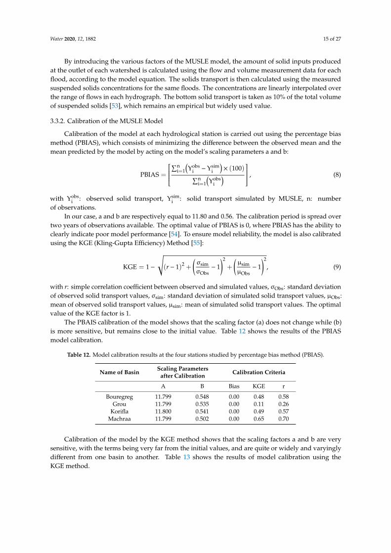
By introducing the various factors of the MUSLE model, the amount of solid inputs producedat the outlet of each watershed is calculated using the flow and volume measurement data for eachflood, according to the model equation. The solids transport is then calculated using the measuredsuspended solids concentrations for the same floods. The concentrations are linearly interpolated overthe range of flows in each hydrograph. The bottom solid transport is taken as 10% of the total volumeof suspended solids [53], which remains an empirical but widely used value.

3.3.2. Calibration of the MUSLE Model

Calibration of the model at each hydrological station is carried out using the percentage biasmethod (PBIAS), which consists of minimizing the difference between the observed mean and themean predicted by the model by acting on the model’s scaling parameters a and b:

PBIAS =

∑n

i=1

(Yobs

i −Ysimi

)× (100)∑n

i=1

(Yobs

i

) , (8)

with Yobsi : observed solid transport, Ysim

i : solid transport simulated by MUSLE, n: numberof observations.

In our case, a and b are respectively equal to 11.80 and 0.56. The calibration period is spread overtwo years of observations available. The optimal value of PBIAS is 0, where PBIAS has the ability toclearly indicate poor model performance [54]. To ensure model reliability, the model is also calibratedusing the KGE (Kling-Gupta Efficiency) Method [55]:

KGE = 1−

√(r− 1)2 +

(σsim

σObs− 1

)2

+

(µsim

µObs− 1

)2

, (9)

with r: simple correlation coefficient between observed and simulated values, σObs: standard deviationof observed solid transport values, σsim: standard deviation of simulated solid transport values, µObs:mean of observed solid transport values, µsim: mean of simulated solid transport values. The optimalvalue of the KGE factor is 1.

The PBAIS calibration of the model shows that the scaling factor (a) does not change while (b)is more sensitive, but remains close to the initial value. Table 12 shows the results of the PBIASmodel calibration.

Table 12. Model calibration results at the four stations studied by percentage bias method (PBIAS).

Name of Basin Scaling Parametersafter Calibration Calibration Criteria

A B Bias KGE r

Bouregreg 11.799 0.548 0.00 0.48 0.58Grou 11.799 0.535 0.00 0.11 0.26

Korifla 11.800 0.541 0.00 0.49 0.57Machraa 11.799 0.502 0.00 0.65 0.70

Calibration of the model by the KGE method shows that the scaling factors a and b are verysensitive, with the terms being very far from the initial values, and are quite or widely and varyinglydifferent from one basin to another. Table 13 shows the results of model calibration using theKGE method.

Water 2020, 12, 1882 16 of 27

Table 13. Model calibration results for the four stations studied by KGE.

Name of Basin Scaling Parametersafter Calibration Calibration Criteria

A b Bias KGE r

Bouregreg 0.039 0.807 0.024 0.601 0.603Grou 11.799 0.546 −0.236 0.149 0.272

Korifla 1.727 0.643 −0.055 0.537 0.545Machraaf 1.421 0.620 −0.017 0.689 0.690

3.4. Comparison of Observations with MUSLE Model Results

3.4.1. Aguibat Zear Hydrological Station on the Bouregreg River

During the two hydrological years studied, twenty-seven floods were recorded. The total solidvolumes observed were 742,334 tons in 2016/2017 and 439,735 tons in 2017/2018. Table 14 summarizesthe results from applying the model to the Aguibat Zear hydrological station.

Table 14. Results of the MUSLE model at Aguibat Zear on the Bouregreg and a comparisonwith observations.

HydrologicYear

Observed SolidTransport

(tons)

Solid Transport(MUSLE)

(tons)

DifferenceObservation-MUSLE

(%)

Uncalibrated CalibrationPBAIS

CalibrationKGE Uncalibrated Calibration

PBAISCalibration

KGE

2016/2017 742 334 619 023 487 494 436 922 −17 −34 −412017/2018 439 735 888 011 694 575 716 809 +102 +58 +63

Examination of the results of the MUSLE model calibrated by the two approaches—PBAIS andKGE—shows that calibration by the PBAIS method better simulates solid transport. Figure 9 comparesthe simulated and observed solid transport. The latter events are less well simulated by MUSLE thanthe former.


Machraaf 1.421 0.620 −0.017 0.689 0.690

3.4. Comparison of Observations with MUSLE Model Results

3.4.1. Aguibat Zear Hydrological Station on the Bouregreg River

During the two hydrological years studied, twenty-seven floods were recorded. The total solid volumes observed were 742,334 tons in 2016/2017 and 439,735 tons in 2017/2018. Table 14 summarizes the results from applying the model to the Aguibat Zear hydrological station.

Table 14. Results of the MUSLE model at Aguibat Zear on the Bouregreg and a comparison with observations.

Hydrologic Year

Observed Solid Transport

(tons)

Solid Transport (MUSLE)

(tons)

Difference Observation-MUSLE

(%)

Uncalibrated Calibration PBAIS

Calibration KGE

Uncalibrated Calibration

PBAIS Calibration

KGE 2016/2017 742 334 619 023 487 494 436 922 −17 −34 −41 2017/2018 439 735 888 011 694 575 716 809 +102 +58 +63

Examination of the results of the MUSLE model calibrated by the two approaches—PBAIS and KGE—shows that calibration by the PBAIS method better simulates solid transport. Figure 9 compares the simulated and observed solid transport. The latter events are less well simulated by MUSLE than the former.

Figure 9. Comparison between MUSLE and observations at Aguibat Zear on the Bouregreg.

3.4.2. Ras Fathia hydrological station on the Grou River

During the two hydrological years studied, twenty-one floods were recorded. The total observed solid volumes amount to 517,194 tons in 2016/2017 and 896,438 tons in 2017/2018. Table 15 summarizes the results of applying the model to the Ras Fathia hydrological station for the two versions of the model calibration.

0

50000

100000

150000

200000

250000

300000

350000

400000

1 2 3 4 5 6 7 8 9 10 11 12 13 14 15 16 17 18 19 20 21 22 23 24 25 26 27

Solid

tran

spor

t in

tons

Flood events

Observed solid transport Solid transport (MUSLE) Solid transport (MUSLE_Calibrated)Figure 9. Comparison between MUSLE and observations at Aguibat Zear on the Bouregreg.

Water 2020, 12, 1882 17 of 27

3.4.2. Ras Fathia Hydrological Station on the Grou River

During the two hydrological years studied, twenty-one floods were recorded. The total observedsolid volumes amount to 517,194 tons in 2016/2017 and 896,438 tons in 2017/2018. Table 15 summarizesthe results of applying the model to the Ras Fathia hydrological station for the two versions of themodel calibration.

Table 15. Results of the MUSLE model at Ras Fathia on the Grou and comparison with observations.

HydrologicYear


(tons)


(tons)


(%)



PBAISCalibration

KGE2016/2017 673 551 875 366 517 194 649 389 +30 −23 −42017/2018 740 083 1 446 831 896 438 1 098 213 +95 +21 +48

Examination of the results of the MUSLE model calibrated by the two approaches PBAIS andKGE, shows that calibration by the PBAIS method better simulates solid transport. Figure 10 showsthe comparison of simulated and observed solid transport. As for the Bouregreg, the events of thesecond year are less well represented by MUSLE.


Table 15. Results of the MUSLE model at Ras Fathia on the Grou and comparison with observations.

Hydrologic Year

Observed Solid

Transport (tons)


(tons)


(%)

Uncalibrated Calibration PBAIS

Calibration KGE Uncalibrated Calibration

PBAIS Calibration

KGE 2016/2017 673 551 875 366 517 194 649 389 +30 −23 −4 2017/2018 740 083 1 446 831 896 438 1 098 213 +95 +21 +48

Examination of the results of the MUSLE model calibrated by the two approaches PBAIS and KGE, shows that calibration by the PBAIS method better simulates solid transport. Figure 10 shows the comparison of simulated and observed solid transport. As for the Bouregreg, the events of the second year are less well represented by MUSLE.

Figure 10. Comparison between MUSLE and observations at Ras Fathia on the Grou.

3.4.3. Sidi Mohamed Cherif Hydrological Station on the Machraa River

During the two hydrological years studied, twelve floods were recorded. The total solid volumes observed were 28,155 tons in 2016/2017 and 48,422 tons in 2017/2018. Table 16 summarizes the results of the application of the model to the hydrological station Sidi Mohamed Cherif.

Table 16. Results of the MUSLE model at Sidi Mohamed Cherif on the Machraa and comparison with observations.

Hydrologic Year

Observed Solid Transport

(tons)


(tons)


(%)


PBAIS Calibration

KGE Uncalibrated

Calibration PBAIS

Calibration KGE

2016/2017 28,155 75,194 27,431 26,225 +167 −3 −7 2017/2018 48,422 141,249 49,146 51,657 +192 +1 +7

0

100000

200000

300000

400000

500000

600000

1 2 3 4 5 6 7 8 9 10 11 12 13 14 15 16 17 18 19 20 21

Solid

tran

spor

t in

tons

Flood events

Observed solid transport Solid transport (MUSLE) Solid transport (MUSLE_Calibrated)

Figure 10. Comparison between MUSLE and observations at Ras Fathia on the Grou.

3.4.3. Sidi Mohamed Cherif Hydrological Station on the Machraa River

During the two hydrological years studied, twelve floods were recorded. The total solid volumesobserved were 28,155 tons in 2016/2017 and 48,422 tons in 2017/2018. Table 16 summarizes the resultsof the application of the model to the hydrological station Sidi Mohamed Cherif.

Water 2020, 12, 1882 18 of 27

Table 16. Results of the MUSLE model at Sidi Mohamed Cherif on the Machraa and comparisonwith observations.

HydrologicYear


(tons)


(tons)


(%)



PBAISCalibration

KGE2016/2017 28,155 75,194 27,431 26,225 +167 −3 −72017/2018 48,422 141,249 49,146 51,657 +192 +1 +7

Examination of the results of the MUSLE model calibrated by the two approaches—PBAIS andKGE—shows that calibration by the PBAIS method better simulates solid transport. Figure 11 shows thecomparison of simulated and observed solid transport. Again, the MUSLE simulations are significantlytoo high for the events in the recording portion.


Examination of the results of the MUSLE model calibrated by the two approaches—PBAIS and KGE—shows that calibration by the PBAIS method better simulates solid transport. Figure 11 shows the comparison of simulated and observed solid transport. Again, the MUSLE simulations are significantly too high for the events in the recording portion.

Figure 11. Comparison between MUSLE and observations at Sidi Mohamed Cherif on the Machraa.

3.4.4. Ain Loudah Hydrological Station on the Korifla River

During the two hydrological years studied, twenty-seven floods were recorded. The total solid volumes observed were 68,759 tons in 2016/2017 and 92,324 tons in 2017/2018. Table 17 summarizes the results of the application of the model to the Ain Loudah hydrological station.

Table 17. Results of the MUSLE model at Ain Loudah on the Korifla and comparison with observations.

Hydrologic Year

Observed Solid

Transport (tons)


(tons)


(%)


PBAIS Calibration

KGE Uncalibrated Calibration

PBAIS Calibration

KGE 2016/2017 68,759 41,083 28,881 27,739 −40 −58 −60 2017/2018 92,324 191,859 132,202 142,138 +108 +43 +54

Examination of the results of the MUSLE model calibrated by the two approaches PBAIS and KGE, shows that calibration by the PBAIS method better simulates solid transports. Figure 12 shows the comparison of simulated and observed solid transports. Out of the four stations studied, it is on the Korifla at Ain Loudah that the simulations seem to be the most efficient.

0

5000

10000

15000

20000

25000

30000

35000

40000

45000

1 2 3 4 5 6 7 8 9 10 11 12

Solid

tran

spor

t in

tons

Flood eventsObserved solid transport Solid transport (MUSLE) Solid transport (MUSLE_Calibrated)

Figure 11. Comparison between MUSLE and observations at Sidi Mohamed Cherif on the Machraa.

3.4.4. Ain Loudah Hydrological Station on the Korifla River

During the two hydrological years studied, twenty-seven floods were recorded. The total solidvolumes observed were 68,759 tons in 2016/2017 and 92,324 tons in 2017/2018. Table 17 summarizesthe results of the application of the model to the Ain Loudah hydrological station.

Table 17. Results of the MUSLE model at Ain Loudah on the Korifla and comparison with observations.

HydrologicYear


(tons)


(tons)


(%)



PBAISCalibration

KGE2016/2017 68,759 41,083 28,881 27,739 −40 −58 −602017/2018 92,324 191,859 132,202 142,138 +108 +43 +54

Examination of the results of the MUSLE model calibrated by the two approaches PBAIS andKGE, shows that calibration by the PBAIS method better simulates solid transports. Figure 12 showsthe comparison of simulated and observed solid transports. Out of the four stations studied, it is onthe Korifla at Ain Loudah that the simulations seem to be the most efficient.

Water 2020, 12, 1882 19 of 27Water 2020, 12, x FOR PEER REVIEW 19 of 26

Figure 12. Comparison between MUSLE and observations at Ain Loudah on the Korifla.

From the deviations from observations at the four hydrological stations, it can be deduced that in general, the model calibrated by the PBAIS method gives better results than the model calibrated by the KGE method. Thus, from the observation we note that the differences varied between −58% and +58% for the model calibrated by PBAIS, between −60% and +63% for the model calibrated by the KGE method, and between −40% and +192% for the model not calibrated.

3.5. Comparison of Observations and Results of the MUSLE Model at the fourHydrological Stations Upstream fromthe SMBA Dam, with BathymetricData

To validate the calibration method, the Nash and Sutcliffe NSE index was used to measure the performance of the model. According to Nash–Sutcliffe [58], NSE is defined as: = 1 − ∑ ( )∑ ( ) , (5)

With NSE: Nash coefficient, Y : observed solid transport, Y : solid transport simulated by MUSLE, µObs: average of the observed solid transport values.

The NSE index varies from −∞ to 1, such that if NSE=1, then the modeled values match the observations perfectly, while a value above 0 shows a relationship between simulation and reality, and a value below 0 shows that there is no relationship between the two. In other words, the closer the efficiency is to 1, the more the model is observed to be accurate.

Table 18 shows the different calculated values of the Nash–Sutcliffe index, which compares observations to the values calculated by the uncalibrated MUSLE model and observations to the values of the calibrated MUSLE model.

Table 18. Nash–Sutcliffe index (NSE) at study stations.

Name of Basin Scaling Parameters after Calibration Nash–Sutcliffe Index (NSE)

a B MUSLE MUSLE calibrated Bouregreg à Aguibat Zear 11.799 0.548 0.38 0.46

Grou à Ras Fathia 11.799 0.535 −0.07 0.02 Korifla à Ain Loudah 11.800 0.541 −0.35 0.30

Machraa à Sidi Mohammed Cherif 11.799 0.502 −9.8 0.47

0

5000

10000

15000

20000

25000

30000

35000

40000

45000

50000

1 2 3 4 5 6 7 8 9 10 11 12 13 14 15 16 17 18 19 20 21 22

Solid

tran

spor

t in

tons

Flood events

Observed solid transport Solid transport (MUSLE) Solid transport (MUSLE_Calibrated)

Figure 12. Comparison between MUSLE and observations at Ain Loudah on the Korifla.

From the deviations from observations at the four hydrological stations, it can be deduced that ingeneral, the model calibrated by the PBAIS method gives better results than the model calibrated bythe KGE method. Thus, from the observation we note that the differences varied between −58% and+58% for the model calibrated by PBAIS, between −60% and +63% for the model calibrated by theKGE method, and between −40% and +192% for the model not calibrated.

3.5. Comparison of Observations and Results of the MUSLE Model at the Four Hydrological Stations Upstreamfrom the SMBA Dam, with Bathymetric Data

To validate the calibration method, the Nash and Sutcliffe NSE index was used to measure theperformance of the model. According to Nash–Sutcliffe [56], NSE is defined as:

NSE = 1−

∑ni=1

(Yobs

i −YSimi

)2

∑ni=1 (Y

obsi − µObs)

2 , (10)

With NSE: Nash coefficient, Yobsi : observed solid transport, Ysim

i : solid transport simulated byMUSLE, µObs: average of the observed solid transport values.

The NSE index varies from −∞ to 1, such that if NSE = 1, then the modeled values match theobservations perfectly, while a value above 0 shows a relationship between simulation and reality, anda value below 0 shows that there is no relationship between the two. In other words, the closer theefficiency is to 1, the more the model is observed to be accurate.

Table 18 shows the different calculated values of the Nash–Sutcliffe index, which comparesobservations to the values calculated by the uncalibrated MUSLE model and observations to the valuesof the calibrated MUSLE model.

Water 2020, 12, 1882 20 of 27

Table 18. Nash–Sutcliffe index (NSE) at study stations.

Name of Basin Scaling Parametersafter Calibration Nash–Sutcliffe Index (NSE)

a B MUSLE MUSLE calibratedBouregreg à Aguibat Zear 11.799 0.548 0.38 0.46

Grou à Ras Fathia 11.799 0.535 −0.07 0.02Korifla à Ain Loudah 11.800 0.541 −0.35 0.30

Machraa à SidiMohammed Cherif 11.799 0.502 −9.8 0.47

In general, the uncalibrated MUSLE model has negative NSE values except for those in theBouregreg basin, which shows that the model values are far from reality, whereas the NSE values of thecalibrated model are positive, varying between 0.02 and 0.47, which shows that the calibrated model issuperior in reliably representing reality.

Though, for the continuity of the experiment we are continuing the calculation on the four basinsin order to complete the comparisons with the volumes of sediment deduced from the bathymetricmeasurements carried out in the SMBA dam reservoir. For the calculation of the volume of suspendedmatter, an earthy density of 1.5 t/m3 is adopted [57]. The siltation of the dam is considered to be equal to9.49 × 106 m3/year. Table 19 summarizes the results of the calculations for all the hydrological stations.

Table 19. Summary table of observation results, application of the MUSLE, calibrated MUSLE_ modeland bathymetry for the four sub-basins of the Bouregreg.

Name of Basin Solid Transport 2016/2017 Solid Transport 2017/2018

Observation MUSLE MUSLEcalibrated Observation MUSLE MUSLE

calibratedBouregreg 742,334 619,023 487,494 439,735 888,011 694,575

Grou 673,551 875,366 517,194 740,083 1,446,831 896,438Korifla 68,759 41,083 28,881 92,324 191,859 132,202

Machraa 28,155 75,194 27,431 48,422 141,249 49,146Total (tons) 1,512,799 1,610,666 1,061,000 1,320,564 2,667,950 1,772,361

Total (106 m3) 1.01 1.07 0.71 0.88 1.78 1.18

Thus, the results listed in Tables 19 and 20 show that the calibrated model is closer to themeasurement than the non-calibrated model, and that the observed values of sediment transportat the four stations, which vary between 1.01 × 106 m3 and 0.88 × 106 m3 for the two hydrologicalyears 2016/2017 and 2017/2018 respectively, and remain largely lower than the quantity of sedimentsobtained by bathymetric measurements in the SMBA dam, which is approximately 9.49 × 106 m3.

Table 20. Comparison of observation results, application of the calibrated MUSLE, MUSLE_ model,and bathymetry for the four sub-basins of the Bouregreg during 2016/2017 and 2017/2018.

HydrologicYear

Bathymetry(106 m3)

DifferenceMUSLE/

Observation

DifferenceMUSLE

Calibrated/Observation

DifferenceObservation/Bathymetry

DifferenceMUSLE/

Bathymetry

DifferenceMUSLE

Calibrated/Bathymetry

2016/20179.25

+5% −30% −89% −89% −93%2016/2018 +102% +34% −91% −81% −88%

4. Discussion and Conclusions

The relationships between man, environment, and solid transport are well understood at thespatial scale of catchment areas, and modeling tools using satellite data are particularly suitable [58].The results obtained from the application of the model (MUSLE), show that the soils of the Bouregregcatchment area are affected by several factors engendering erosion, i.e., steep slopes, low vegetation

Water 2020, 12, 1882 21 of 27

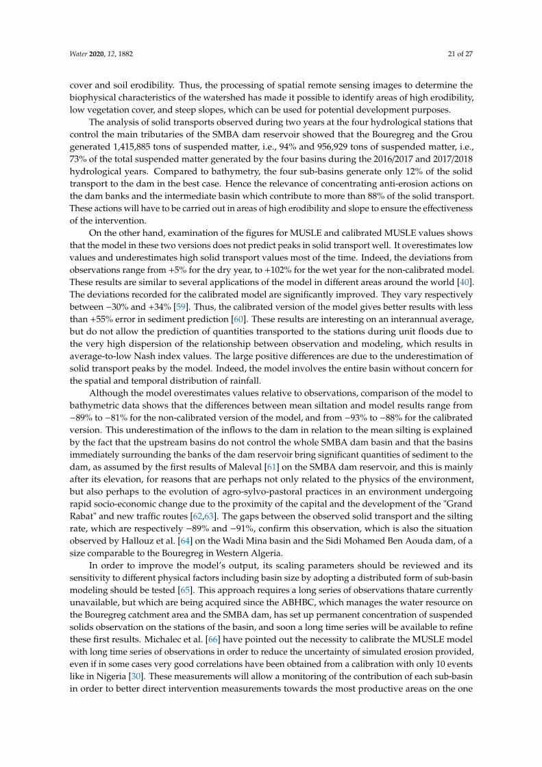
cover and soil erodibility. Thus, the processing of spatial remote sensing images to determine thebiophysical characteristics of the watershed has made it possible to identify areas of high erodibility,low vegetation cover, and steep slopes, which can be used for potential development purposes.

The analysis of solid transports observed during two years at the four hydrological stations thatcontrol the main tributaries of the SMBA dam reservoir showed that the Bouregreg and the Grougenerated 1,415,885 tons of suspended matter, i.e., 94% and 956,929 tons of suspended matter, i.e.,73% of the total suspended matter generated by the four basins during the 2016/2017 and 2017/2018hydrological years. Compared to bathymetry, the four sub-basins generate only 12% of the solidtransport to the dam in the best case. Hence the relevance of concentrating anti-erosion actions onthe dam banks and the intermediate basin which contribute to more than 88% of the solid transport.These actions will have to be carried out in areas of high erodibility and slope to ensure the effectivenessof the intervention.

On the other hand, examination of the figures for MUSLE and calibrated MUSLE values showsthat the model in these two versions does not predict peaks in solid transport well. It overestimates lowvalues and underestimates high solid transport values most of the time. Indeed, the deviations fromobservations range from +5% for the dry year, to +102% for the wet year for the non-calibrated model.These results are similar to several applications of the model in different areas around the world [40].The deviations recorded for the calibrated model are significantly improved. They vary respectivelybetween −30% and +34% [59]. Thus, the calibrated version of the model gives better results with lessthan +55% error in sediment prediction [60]. These results are interesting on an interannual average,but do not allow the prediction of quantities transported to the stations during unit floods due tothe very high dispersion of the relationship between observation and modeling, which results inaverage-to-low Nash index values. The large positive differences are due to the underestimation ofsolid transport peaks by the model. Indeed, the model involves the entire basin without concern forthe spatial and temporal distribution of rainfall.

Although the model overestimates values relative to observations, comparison of the model tobathymetric data shows that the differences between mean siltation and model results range from−89% to −81% for the non-calibrated version of the model, and from −93% to −88% for the calibratedversion. This underestimation of the inflows to the dam in relation to the mean silting is explainedby the fact that the upstream basins do not control the whole SMBA dam basin and that the basinsimmediately surrounding the banks of the dam reservoir bring significant quantities of sediment to thedam, as assumed by the first results of Maleval [61] on the SMBA dam reservoir, and this is mainlyafter its elevation, for reasons that are perhaps not only related to the physics of the environment,but also perhaps to the evolution of agro-sylvo-pastoral practices in an environment undergoingrapid socio-economic change due to the proximity of the capital and the development of the "GrandRabat" and new traffic routes [62,63]. The gaps between the observed solid transport and the siltingrate, which are respectively −89% and −91%, confirm this observation, which is also the situationobserved by Hallouz et al. [64] on the Wadi Mina basin and the Sidi Mohamed Ben Aouda dam, of asize comparable to the Bouregreg in Western Algeria.

In order to improve the model’s output, its scaling parameters should be reviewed and itssensitivity to different physical factors including basin size by adopting a distributed form of sub-basinmodeling should be tested [65]. This approach requires a long series of observations thatare currentlyunavailable, but which are being acquired since the ABHBC, which manages the water resource onthe Bouregreg catchment area and the SMBA dam, has set up permanent concentration of suspendedsolids observation on the stations of the basin, and soon a long time series will be available to refinethese first results. Michalec et al. [66] have pointed out the necessity to calibrate the MUSLE modelwith long time series of observations in order to reduce the uncertainty of simulated erosion provided,even if in some cases very good correlations have been obtained from a calibration with only 10 eventslike in Nigeria [30]. These measurements will allow a monitoring of the contribution of each sub-basinin order to better direct intervention measurements towards the most productive areas on the one

Water 2020, 12, 1882 22 of 27

hand, thus reducing the overall cost of the measures to reduce erosion, and to improve modeling andsubsequent solid transport forecasting on the other hand.

Eventually, the results of the MUSLE model confirm the relevance of its application in watershedmanagement studies once calibrated, since it integrates all forms of erosion observed at the watershedscale, coupled with hydrological data, which greatly improves accuracy compared to USLE [67] and toRUSLE [68]. Indeed, the average specific degradation at the level of the Bouregreg basin alone at theAguibat Zear station is of the order of 13.81 t/ha/year according to Moussebbih et al. [69] when calculatedby the RUSLE method, whereas those of calibrated MUSLE and observation are of the order of 1.6t/ha/year. The studies carried out on the wadi Mina basin in Algeria, a basin similar to the Bouregregbasin [64], confirm this finding with deviations of the RUSLE model results from the measurementof suspended solids concentrations, which can reach 79%. In Spain, Ramos-Diez et al. [70] have usedthe USLE formula to assess the amount of sediment inputs to 25 very small check dams used in animportant restoration project over a 9 km2 area in the north of Spain, showing interesting but stillmitigated results and concluding that the size and shape of the dams had an impact on the quality ofthe USLE assessment.

Kronvang et al. [71] showed that bank erosion was the dominant sediment source (90–94%) in theRiver Odense catchment in Denmark during three study years. They add that in-channel and overbanksediment sinks and storage dominated the sediment budget, as 79–94% of the sediment input fromall sources was not exported from the catchment during the three study years. This is in accordancewith our results, as the regular bathymetric survey to monitor the silting up rate of the dam haveshown that half of the sediment input to the reservoir comes from the dam banks. Our results are veryimportant for the forthcoming works for erosion mitigation on the Bouregreg catchment; they willenable more efficient orientation of the soil conservation and restoration works that may be carriedout in the future, with priority being given to the environment close to the dam, in order to preservethe water capacity of the SMBA dam reservoir while optimizing the financial resources mobilized.Palazon and Navas [72] have shown the same interest to monitor the sediment sources draining to alarge reservoir in the Esera River, Ebro basin in Spain. The small basin size (1500 km2) allowed them touse the SWAT model as an alternative to MUSLE with two gauging stations, each one being covered bydifferent types of soil. This might make it possible to implement the SWAT model on the Bouregregbasin, when the ABHBC will have started the monitoring of sediment transport at all the stations ofthe basin.

To conclude, it should be pointed out that in the context of climate change, which predicts, inMorocco, an increase in temperatures and a drop in rainfall [73–75], the projections of erosion andsediment transport evolution that are possible from climate model outputs, and which are based onUSLE or SWAT type approximation models [76], will need observed data to calibrate and validatetheir results.

Author Contributions: Conceptualization, M.A.E. and G.M.; methodology, M.A.E.; software, M.A.E.; validation,G.M., I.K. and A.Z.; formal analysis, M.A.E.; investigation, M.A.E.; resources, A.Z.; data curation, A.Z.;writing—original draft preparation, M.A.E. and G.M.; writing—review and editing, M.A.E.; visualization,M.A.E.; supervision, G.M., I.K. and A.Z.; project administration, G.M., I.K. and A.Z. All authors have read andagreed to the published version of the manuscript.

Funding: This research received no external funding.

Acknowledgments: Thanks to ABHBC for the hydrological and rainfall data.

Conflicts of Interest: The authors declare no conflict of interest.

References

1. Mahe, G.; Emran, A.; Brou, Y.T.; Tra Bi, A.Z. Analyse statistique de l’évolution de la couverture végétale àpartir d’images MODIS et NOAA sur le bassin versant du Bouregreg (Maroc). Géo Obs. 2012, 20, 33–44.

Water 2020, 12, 1882 23 of 27

2. Laouina, A.; Aderghal, M.; Al Karkouri, J.; Antari, M.; Chaker, M.; Laghazi, Y.; Machmachi, I.; Machouri, N.;Nafaa, R.; Naïmi, K. The efforts for cork oak forest management and their effects on soil conservation.For. Syst. 2010, 19, 263–277. [CrossRef]

3. Schmidt, S.; Alewell, C.; Meusburger, K. Monthly RUSLE soil erosion risk of Swiss grasslands. J. Maps 2019,15, 247–256. [CrossRef]

4. Yahiaoui, S.; Zerouali, A. Etude de l’évolution de l’occupation du sol sur deux grands bassins d’Algérie et duMaroc, et relation avec la sédimentation dans les barrages. In Considering Hydrological Change in ReservoirPlanning and Management; IAHS Publ 362; Schumann, A., Belyaev, V.B., Gargouri, E., Kucera, G., Mahe, G.,Eds.; IAHS Press: Wallingford, UK, 2013; pp. 115–124.

5. Khomsi, K.; Mahe, G.; Sinan, M.; Snoussi, M. Hydro-climatic variability in two Moroccan watersheds: Acomparative analysis of temperature, rain and flow regimes. In Climate and Land Surface Changes in Hydrology;IAHS Publ. 359; Boegh, E., Blyth, E., Hannah, D.M., Hisdal, H., Kunstmann, H., Su, B., Yilmaz, K.K., Eds.;IAHS Press: Wallingford, UK, 2013; pp. 183–190.

6. Khomsi, K.; Mahe, G.; Tramblay, Y.; Sinan, M.; Snoussi, M. Regional impacts of global change: Seasonaltrends in extreme rainfall, runoff and temperature in two contrasted regions of Morocco. Nat. Hazards EarthSyst. Sci. 2016, 16, 1079–1090. [CrossRef]

7. Mahe, G.; Emran, A.; Brou, Y.T.; Tra Bi, A.Z. Impact de la variabilité climatique sur l’état de surface du bassinversant du Bouregreg (Maroc). Eur. J. Sci. Res. 2012, 84, 417–425.

8. ABV. Plan National d’Aménagement des Bassins Versant; Haut-Commissariat aux Eaux et Forêts et à la LutteContre la Désertification: Rabat, Morocco, 1996.

9. Wischmeier, W.H.; Smith, D.D. Predicting Rainfall-Erosion Losses from Cropland East of the Rocky Mountains:Guide for Selection of Practices for Soil and Water Conservation; US Department of Agriculture: Washington, DC,USA, 1965.

10. Williams, J.R. Sediment-Yield Prediction with Universal Equation Using Runoff Energy Factor; ARS-S. SouthernRegion, Agricultural Research Service, US Department of Agriculture: Washington, DC, USA, 1975;Volume 40, p. 244.

11. El Bahi, S.; El Wartiti, M.; Yassin, M.; Calle, A.; Casanova, J.L. Applying revised universal loss equationmodel to forest lands in Central Plateau of Morocco. Rev. Teledetección 2005, 23, 89–97.

12. Chadli, K. Estimation of soil loss using RUSLE model for Sebou watershed (Morocco). Model. EarthSyst. Environ. 2016, 2, 51. [CrossRef]

13. Elaloui, A.; Marrakchi, C.; Fekri, A.; Maimouni, S.; Aradi, M. USLE-based assessment of soil erosion by waterin the watershed upstream Tessaoute (Central High Atlas, Morocco). Modeling Earth Syst. Environ. 2017, 3,873–885. [CrossRef]

14. Hara, F.; Achab, M.; Emran, A.; Mahe, G.; Fhel, B.E. Estimate the Risk of Soil Erosion Using USLE throughthe Development of an Open Source Desktop Application: DUSLE (Desktop Universal Soil Loss Equation).In Proceedings of the 3rd International Conference on African Large River Basin Hydrology, Alger, Algeria,May 2018; Available online: https://hal.archives-ouvertes.fr/hal-02397686/ (accessed on 17 June 2020).

15. Boufala, M.; El Hmaidf, A.; Chadli, K.; Essahlaoui, A.; El Ouali, A.; Lahjouj, A. Assessment of the Riskof Soil Erosion Using RUSLE Method and SWAT Model at the M’dez Watershed, Middle Atlas, Morocco.In Proceedings of the E3S Web Conf., The Seventh International Congress “Water, Waste and Environment”(EDE7-2019), Salé, Morocco, 20–22 November 2019; Volume 150. [CrossRef]

16. Toumi, S.; Meddi, M.; Mahe, G.; Brou, Y.T. Cartographie de l’érosion dans le bassin versant de l’Oued Minaen Algérie par télédétection et SIG. Hydrol. Sci. J. 2013, 58, 1–17. [CrossRef]

17. Mihi, A.; Benarfa, N.; Arar, A. Assessing and mapping water erosion-prone areas in northeastern Algeriausing analytic hierarchy process, USLE/RUSLE equation, GIS, and remote sensing. Appl. Geomat. 2019.[CrossRef]

18. Gaubi, I.; Chaabani, A.; Ben Mammou, A.; Hamza, M.H. A GIS-based soil erosion prediction using theRevised Universal Soil Loss Equation (RUSLE) (Lebna watershed, Cap Bon, Tunisia). Nat. Hazards 2017, 86,219–239. [CrossRef]

19. Toubal, A.K.; Achite, M.; Ouillon, S.; Dehni, A. Soil erodibility mapping using the RUSLE model to prioritizeerosion control in the Wadi Sahouat basin. North-West Alger. Environ. Monit. Assess. 2018, 190, 4. [CrossRef][PubMed]

http://dx.doi.org/10.5424/fs/2010192-01320

http://dx.doi.org/10.1080/17445647.2019.1585980

http://dx.doi.org/10.5194/nhess-16-1079-2016

http://dx.doi.org/10.1007/s40808-016-0105-y

http://dx.doi.org/10.1007/s40808-017-0340-x

https://hal.archives-ouvertes.fr/hal-02397686/

http://dx.doi.org/10.1051/e3sconf/202015003014

http://dx.doi.org/10.1080/02626667.2013.824088

http://dx.doi.org/10.1007/s12518-019-00289-0

http://dx.doi.org/10.1007/s11069-016-2684-3

http://dx.doi.org/10.1007/s10661-018-6580-z

http://www.ncbi.nlm.nih.gov/pubmed/29532173

Water 2020, 12, 1882 24 of 27

20. El Aroussi, O.; Mesrar, L.; El Garouani, A.; Lahrach, A.; Beaabidaate, L.; Akdi, B.; Jabrane, R. Predictingthe potential annual soil loss using the revised universal soil loss equation (RUSLE) in the oued El Mallehcatchment (Prerif, Morocco). Present. Environ. Sustain. Dev. 2011, 5, 5–16.

21. Lamyaa, K.; M’bark, A.; Brahim, I.; Hicham, A.; Soraya, M. Mapping Soil Erosion Risk Using RUSLE, GIS,Remote Sensing Methods: A Case of Mountainous Sub-watershed, Ifni Lake and High Valley of Tifnoute(High Moroccan Atlas). J. Geogr. Environ. Earth Sci. Int. 2018, 14, 1–11. [CrossRef]

22. Bagarello, V.; Ferro, V.; Giordano, G.; Mannocchi, F.; Todisco, F.; Vergni, L. Statistical check of USLE-M andUSLE-MM to predict bare plot soil loss in two Italian environments. Land Degrad. Dev. 2018, 29, 2614–2628.[CrossRef]

23. Wischmeier, W.H.; Smith, D.D. Predicting Rainfall Erosion Losses: A Guide to Conservation Planning; Departmentof Agriculture, Science and Education Administration: Washington, DC, USA, 1978.

24. Renard, K.G. Predicting Soil Erosion by Water: A Guide to Conservation Planning with the Revised Universal SoilLoss Equation (RUSLE); United States Government Printing: Washington, DC, USA, 1997.

25. Kinnell, P.I.A. Why the Universal Soil Loss Equation and the Revised Version of It Do Not Predict EventErosion Well. Hydrol. Process. 2005, 19, 851–854. [CrossRef]

26. Haan, C.T.; Barfield, B.J.; Hayes, J.C. Design Hydrology and Sedimentology for Small Catchments.J. Hydrol. -Amst. 1963, 176, 296–297.

27. Novotny, V. Water Quality: Prevention, Identification and Management of Diffuse Pollution; Van Nostrand-ReinholdPublishers: New York, NY, USA, 1994; ISBN 978-0442005597.

28. Alewell, C.; Borrelli, P.; Meusburger, K.; Panagos, P. Using the USLE: Chances, challenges and limitations ofsoil erosion modelling. Int. Soil Water Conserv. Res. 2019, 7, 203–225. [CrossRef]

29. Odongo, V.O.; Onyando, J.O.; Mutua, B.M.; van Oel, P.R.; Becht, R. Sensitivity analysis and calibrationof the Modified Universal Soil Loss Equation (MUSLE) for the upper Malewa Catchment, Kenya. Int. J.Sediment Res. 2013, 28, 368–383. [CrossRef]

30. Adegede, A.P.; Mbajiorgu, C.C. Event-based sediment yield modeling for small watersheds using MUSLE innorth-central Nigeria. Agric. Eng. Int.: CIGR J. 2019, 21, 7–17.

31. Yassin, M.; Pépin, Y.; El Bahi, S.; Zante, P. Evaluation de l’érosion au micro-bassin de Sidi Sbaa: Applicationdu modèle MUSLE. Ann. Rech. For. Maroc 2013, 42, 171–181.

32. Samaras, A.G.; Koutitas, C.G. Modeling the impact of climate change on sediment transport and morphologyin coupled watershed-coast systems: A case study using an integrated approach. Int. J. Sediment Res. 2014,29, 304–315. [CrossRef]

33. Fang, H. Impact of land use changes on catchment soil erosion and sediment yield in the northeastern China:A panel data model application. Int. J. Sediment Res. 2020. [CrossRef]

34. Djoukbala, O.; Hasbaia, M.; Benselama, O.; Mazour, M. Comparison of the erosion prediction models fromUSLE, MUSLE and RUSLE in a Mediterranean watershed, case of Wadi Gazouana (N-W of Algeria). ModelingEarth Syst. Environ. 2018. [CrossRef]

35. Mahe, G.; Benabdelfadel, H.; Dieulin, C.; Elbaraka, M.; Ezzaouini, M.; Khomsi, K.; Rouche, N.; Sinan, M.;Snoussi, M.; Tra Bi, A.; et al. Evolution des débits liquides et solides du Bouregreg. In Gestion Durable desTerres. Proceedings de la Réunion Multi-Acteurs Sur le Bassin du Bouregreg. CERGéo, Faculté des Lettres et SciencesHumaines, Université Mohammed V-Agdal, Rabat, 28 mai 2013; Laouina, A., Mahe, G., Eds.; Edité par ARGDT:Rabat, Morocco, 2014; pp. 21–36, ISBN 978-9954-33-482-9.

36. Khali Issa, L.; Ben Hamman Lech-Hab, K.; Raissouni, A.; El Arrim, A. Cartographie quantitative du risqued’érosion des sols par approche SIG/USLE au niveau du bassin versant Kalaya (Maroc Nord Occidental).J. Mater. Environ. Sci. 2016, 7, 2778–2795.

37. El Jazouli, A.; Barakat, A.; Ghafiri, A.; El Moutaki, S.; Ettaqy, A.; Khellouk, R. Soil erosion modeled withUSLE, GIS, and remote sensing: A case study of Ikkour watershed in Middle Atlas (Morocco). Geosci. Lett.2017, 4, 1. [CrossRef]

38. Sabri, E. Impact des Processus Erosifs sur les Ressources Naturelles des Bassins Hydrographiques et surL’état D’envasement des Retenues des Barrages: Application au Bassin Versant de L’oued El Abid en Amontdu Barrage de Bin El Ouidane- Maroc. Ph.D. Thesis, Univ. Cadi Ayyad, Marrakech, Morocco, 2018.

39. Sadeghi, S.H.R.; Gholami, L.; Khaledi Darvishan, A.; Saeidi, P. A review of the application of the MUSLEmodel worldwide. Hydrol. Sci. J. 2014, 59, 365–375. [CrossRef]

http://dx.doi.org/10.9734/JGEESI/2018/40322

http://dx.doi.org/10.1002/ldr.3072

http://dx.doi.org/10.1002/hyp.5816

http://dx.doi.org/10.1016/j.iswcr.2019.05.004

http://dx.doi.org/10.1016/S1001-6279(13)60047-5

http://dx.doi.org/10.1016/S1001-6279(14)60046-9

http://dx.doi.org/10.1016/j.ijsrc.2020.03.017

http://dx.doi.org/10.1007/s40808-018-0562-6

http://dx.doi.org/10.1186/s40562-017-0091-6

http://dx.doi.org/10.1080/02626667.2013.866239

Water 2020, 12, 1882 25 of 27

40. Aboulabbes, O. Infiltration Characteristics on a Small Watershed. Master’s Thesis, Utah State University,Logan Utah, UT, USA, 1984.

41. El Gaatib, R.; Erraji, A.; Larabi, A. Impact des processus érosifs sur les ressources naturelles des bassinshydrographiques et sur l’état d’envasement des retenues de barrages: Application au Bassin Versant del’Oued Beht en amont du barrage El Kansra, (Maroc). Géo Obs. 2014, 21, 4.

42. Jamagne, M. Bases et Techniques d’une Cartographie des Sols’; Institut National de la Recherche Agronomique:Paris, France, 1967.

43. Stone, R.P.; Hilborn, D. Universal Soil Loss Equation, USLE; Factsheet; Government of Ontario, Ministry ofAgriculture, Food and Rural Affairs: Canada, 2000. Available online: http://www.omafra.gov.on.ca/english/

engineer/facts/12-051.htm (accessed on 17 June 2020).44. Pribyl, D.W. A critical review of the conventional SOC to SOM conversion factor. Geoderma 2010, 156, 75–83.

[CrossRef]45. Van Bemmelen, J.M. “Über die Bestimmung des Wassers, des Humus, des Schwefels, der in den colloïdalen

Silikaten gebundenen Kieselsäure, des Mangansuswim Ackerboden”. Die LandwirthschaftlichenVers.-Stn.1890, 37, 279–290.

46. Wolff, E. Entwurf zur boden analyse. Z. Anal. Chem. 1864, 3, 85–115. [CrossRef]47. Sprengel, C. Ueber Pflanzenhumus, Humussaüre und humussaure Salze. Arch. für die Gesammte 1826, 8,

145–220. [CrossRef]48. Tra Bi, Z.A.; Emran, A.; Brou, Y.T.; Mahé, G. Cartographie par arbre de décision de la dynamique de

l’occupation du sol du bassin versant du Bouregreg, en région semi-aride au centre Nord-Ouest du Maroc,Abidjan, Côte d’Ivoire. Rev. Sci. Int. Géomatique 2014, 1, 43–54.

49. Sadiki, A.; Bouhlassa, S.; Auajjar, J. Utilisation d’un SIG pour l’évaluation et la cartographie des risquesd’érosion par utilisation d’un SIG pour l‘évaluation et la cartographie des risques d’érosion par l’équationuniverselle des pertes en sol dans le Rif oriental (Maroc). Bull. de l’Inst. Sci. 2004, 26, 69–79.

50. Goussot, E.; Brou, Y.T.; Laouina, A.; Chaker, M.; Emran, A.; Machouri, N.; Mahe, G.; Sfa, M.; Tra Bi, A. Landcovers dynamic and agricultural statistics on the Bouregreg watershed in Morocco. Eur. J. Sci. Res. 2014, 126,191–205.

51. Tra Bi, A.Z.; Brou, T.; Emran, A.; Mahe, G. Remote sensing and GIS analysis of the dynamic of vegetation inclimate variability context on the Bouregreg watershed. In Climate and Land Surface Changes in Hydrology;IAHS Publ. 359; Boegh, E., Blyth, D.M., Hannah, H., Hisdal, H., Kunstmann, B., Su, K.K., Yilmaz, Eds.; IAHSPress: Wallingford, UK, 2013; pp. 403–410.

52. El Hadraoui, Y. Étude Diachronique de L’occupation du sol et de Modélisation des Processus Erosifs du BassinVersant du Bouregreg (Maroc) à Partir des Données de L’observation de la Terre; Mémoire d’ingénieur du CNAM,Spécialité Géomètre et Topographe: Le Mans, France, 2013; Available online: https://dumas.ccsd.cnrs.fr/dumas-00920465 (accessed on 17 June 2020).

53. Lahlou, A. La Dégradation Spécifique des Bassins Versants et son Impact sur L’envasement des Barrages; IAHS Publ.137; IAHS Press: Wallingford, UK, 1982; pp. 163–169. Available online: https://pdfs.semanticscholar.org/

cddc/4f4b21f52e34043e1b0547d00d0e9dd389b9.pdf (accessed on 17 June 2020).54. Gupta, H.V.; Sorooshian, S.; Yapo, P.O. Status of automatic calibration for hydrologic models: Comparison

with multilevel expert calibration. J. Hydrol. Eng. 1999, 4, 135–143. [CrossRef]55. Gupta, H.V.; Kling, H.; Yilmaz, K.K.; Martinez, G.F. Decomposition of the mean squared error and NSE

performance criteria: Implications for improving hydrological modelling. J. Hydrol. 2009, 377, 80–91.[CrossRef]

56. Nash, J.E.; Sutcliffe, J.V. River flow forecasting through conceptual models part I—A discussion of principles.J. Hydrol. 1970, 10, 282–290. [CrossRef]

57. Lahlou, A. Etude du transport solide à la station Dar Es Soltane sur l’oued Bouregreg; Rapport de travaux du serviceGDE; Gestion des eaux, Ministère des travaux publics et des communications, Direction de l’hydraulique:Rabat, Morocco, 1971.

58. Mahe, G.; Aksoy, H.; Brou, Y.T.; Meddi, M.; Roose, E. Relationships among man, environment and sedimenttransport: A spatial approach. Rev. Sci. Eau 2013, 26, 235–244. [CrossRef]

59. De Vente, J.; Verduyn, R.; Verstraeten, G.; Vanmaercke, M.; Poesen, J. Factors controlling sediment yield atthe catchment scale in NW Mediterranean geoecosystems. J. Soils Sediments 2011, 11, 690–707. [CrossRef]

http://www.omafra.gov.on.ca/english/engineer/facts/12-051.htm

http://www.omafra.gov.on.ca/english/engineer/facts/12-051.htm

http://dx.doi.org/10.1016/j.geoderma.2010.02.003

http://dx.doi.org/10.1007/BF01345998

http://dx.doi.org/10.1002/ardp.18270210315

https://dumas.ccsd.cnrs.fr/dumas-00920465

https://dumas.ccsd.cnrs.fr/dumas-00920465

https://pdfs.semanticscholar.org/cddc/4f4b21f52e34043e1b0547d00d0e9dd389b9.pdf

https://pdfs.semanticscholar.org/cddc/4f4b21f52e34043e1b0547d00d0e9dd389b9.pdf

http://dx.doi.org/10.1061/(ASCE)1084-0699(1999)4:2(135)

http://dx.doi.org/10.1016/j.jhydrol.2009.08.003

http://dx.doi.org/10.1016/0022-1694(70)90255-6

http://dx.doi.org/10.7202/1018788ar

http://dx.doi.org/10.1007/s11368-011-0346-3

Water 2020, 12, 1882 26 of 27

60. Moriasi, D.N.; Arnold, J.G.; Van Liew, M.W.; Bingner, R.L.; Harmel, R.D.; Veith, T.L. Model evaluationguidelines for systematic quantification of accuracy in watershed simulations. Transactions of the ASABE.Am. Soc. Agric. Biol. Eng. 2007, 50, 885–900.

61. Maleval, V. Premiers résultats des mesures d’érosion ravinaire sur les versants lacustres du barrage SidiMohamed ben Abdellah (Maroc) et perspectives de recherche. In Gestion Durable des Terres. Proceedings de laréunion multi-acteurs sur le bassin du Bouregreg. CERGéo, Faculté des Lettres et Sciences Humaines, UniversitéMohammed V-Agdal, Rabat, 28 mai 2013; Laouina, A., Mahe, G., Eds.; Edité par ARGDT: Rabat, Morocco, 2014;pp. 53–62, ISBN 978-9954-33-482-9.

62. Laouina, A.; Chaker, A.; Aderghal, M.; Machouri, N.; Al Karkouri, J. Echelles d’évaluation de la dynamiquedes terres et de leur gestion, du territoire social au bassin-versant expérimental. In Gestion Durable des Terres.Proceedings de la réunion multi-acteurs sur le bassin du Bouregreg. CERGéo, Faculté des Lettres et Sciences Humaines,Université Mohammed V-Agdal, Rabat, 28 mai 2013; Laouina, A., Mahe, G., Eds.; Edité par ARGDT: Rabat,Morocco, 2014; pp. 119–146, ISBN 978-9954-33-482-9.

63. Chaker, M.; Laouina, A.; El Marbouh, M. Changement agropastoral et dégradation des terres dans le plateauSehoul. In Gestion Durable des Terres. Proceedings de la Réunion Multi-Acteurs sur le Bassin du Bouregreg.CERGéo, Faculté des Lettres et Sciences Humaines, Université Mohammed V-Agdal, Rabat, 28 mai 2013; Laouina, A.,Mahe, G., Eds.; Edité par ARGDT: Rabat, Morocco, 2014; pp. 85–102, ISBN 978-9954-33-482-9.

64. Hallouz, F.; Mahé, G.; Toumi, S.; Rahmani, S.E.A. Erosion, suspended sediment transport and sedimentationon the Wadi Mina at the Sidi M’Hamed Ben Aouda Dam, Algeria. Water 2018, 10, 895. [CrossRef]

65. Gwapedza, D.; Hughes, D.A.; Slaughter, A.R. Spatial scale dependency issues in the application of theModified Universal Soil Loss Equation (MUSLE). Hydrol. Sci. J. 2018, 63, 1890–1900. [CrossRef]

66. Michalec, B.; Walega, A.; Cupak, A.; Strutynski, M. Verification of the musle to determine the amount ofsuspended sediment. Carpathian J. Earth Environ. Sci. 2017, 12, 235–244.

67. Iroumé, A.; Carey, P.; Bronstert, A.; Huber, A.; Palacios, H. GIS application of USLE and MUSLE to estimateerosion and suspended sediment load in experimental catchments, Valdivia, Chile. Aplicación SIG de USLE yMUSLE para Estimar la Erosión y el Transporte de Sedimentos en Suspensión en Cuencasexperimentales 2011, 34,119–128.

68. Arekhi, S.; Shabani, A.; Alavipanah, S.K. Evaluation of integrated KW-GIUH and MUSLE models to predictsediment yield using geographic information system (GIS) (Case study: Kengir watershed, Iran). Afr. J.Agric. Res. 2011, 6, 4185–4198.

69. Moussebbih, A.; Souissi, M.; Larabi, A.; Faouzi, M. Modeling and mapping of the water erosion risk usingGis/Rusle approach in the Bouregreg river watershed. Int. J. Mech. Prod. Eng. Res. Dev. 2019, 9, 1605–1618.[CrossRef]

70. Ramos-Diez, I.; Navarro-Hevia, J.; San Martín, R.; Díaz-Gutiérrez, V.; Mongil-Manso, J. Evaluating methodsto quantify sediment volumes trapped behind check dams, Saldaña badlands (Spain). Int. J. Sediment Res.2016, 28, 2446–2456. [CrossRef]

71. Kronvang, B.; Andersen, H.E.; Larsen, S.E.; Audet, J. Importance of bank erosion for sediment input, storageand export at the catchment scale. J. Soils Sediments 2013, 13, 230–241. [CrossRef]

72. Palazón, L.; Navas, A. Modeling sediment sources and yields in a Pyrenean catchment draining to a largereservoir (Ésera River, Ebro Basin). J. Soils Sediments 2014, 14, 1612–1625. [CrossRef]

73. Driouech, F.; Mahé, G.; Déqué, M.; Dieulin, C.; El Heirech, T.; Milano, M.; Benabdelfadel, H.; Rouché, N.Evaluation d’impacts potentiels de changements climatiques sur l’hydrologie du bassin versant de laMoulouya au Maroc. In Global Change: Facing Risks and Threats to Water Resources. Proceedings of the SixthWorld FRIEND Conference, Fez, Morocco, October 2010; IAHS Publ. 340; IAHS Press: Wallingford, UK,2010; pp. 561–567. Available online: https://horizon.documentation.ird.fr/exl-doc/pleins_textes/divers15-08/

010055009.pdf (accessed on 17 June 2020).74. Filahi, S.; Tramblay, Y.; Mouhir, L.; Diaconescu, E.P. Projected changes in temperature and precipitation

indices in Morocco from high-resolution regional climate models. Int. J. Climatol. 2017, 37, 4846–4863.[CrossRef]

http://dx.doi.org/10.3390/w10070895

http://dx.doi.org/10.1080/02626667.2018.1546388


http://dx.doi.org/10.1016/j.ijsrc.2016.06.005

http://dx.doi.org/10.1007/s11368-012-0597-7

http://dx.doi.org/10.1007/s11368-014-0911-7

https://horizon.documentation.ird.fr/exl-doc/pleins_textes/divers15-08/010055009.pdf

https://horizon.documentation.ird.fr/exl-doc/pleins_textes/divers15-08/010055009.pdf

http://dx.doi.org/10.1002/joc.5127

Water 2020, 12, 1882 27 of 27

75. Tramblay, Y.; Jarlan, L.; Hanich, L.; Somot, S. Future scenarios of surface water resources availability in NorthAfrican dams. Water Resour. Manag. 2018, 32, 1291–1306. [CrossRef]

76. Raclot, D.; Naimi, M.; Chikhaoui, M.; Nunez, J.P.; Huard, F.; Herivaux, C.; Sabir, M.; Pepin, Y. Distinct andcombined impacts of climate and land use scenarios on water availability and sediment loads for a watersupply reservoir in northern Morocco. Int. J. Soil Conserv. 2020. [CrossRef]

© 2020 by the authors. Licensee MDPI, Basel, Switzerland. This article is an open accessarticle distributed under the terms and conditions of the Creative Commons Attribution(CC BY) license (http://creativecommons.org/licenses/by/4.0/).

http://dx.doi.org/10.1007/s11269-017-1870-8


http://creativecommons.org/

http://creativecommons.org/licenses/by/4.0/.

comparison of the musle model and two years of solid

Documents