comparison of techniques for assessing effects of loading uncertainty upon a long term phosphorous...

Comparison of techniques for assessing effects of loading uncertainty upon a long term phosphorous model Ronald Malone

Department of Civil Engineering, Louisiana State University, Baton Rouge, Louisiana, USA

David S. Bowles

Law Engineering and Testing Company, Englewood, Colorado, USA

M. P. Windham

Department of Mathematics, College of Science, Utah State University, Logan, Utah, USA

W. J. Grenney

Department of Civil and Environmental Engineering, College of Engineering, Utah State University, Logan, Utah, USA

(Received November 1981; revised March 1982)

This paper compares the feasibility of applying three stochastic techniques to a linear water quality model. The Monte Carlo, first order analysis, and generation of moment equation techniques are applied to a long term phosphorus model of Lake Washington. The effect of uncertainty of the phosphorus loading term on simulated phosphorus levels is analysed. The simulated concentrations of phosphorus in the water column are very responsive to uncertainty in annual phosphorus loading, but the sediment concentrations are relatively insensitive. All three stochastic techniques produced identical results, but the level of preparatory and computational effort required varies considerably. The Monte Carlo technique requires the most computation time of the three stochastic techniques examined. The first order analysis and generation of moment equation techniques are shown to be precise and efficient methods of stochastic analysis. In this application they required less than one-thousandth the computer time of the Monte Carlo technique

Key words: mathematical model, Monte Carlo technique, linear water quality model

Introduction have inherent limitations when used as management tools. Deterministic models produce a single set of output

This paper compares three stochastic techniques which have variables (effects) from each set of imput variables (causes).’ potential usefulness in the analysis of water quality manage- When water quality systems which are subject to large ment problems in natural systems. These stochastic cyclic and random variations are modelled with imprecise approaches were investigated in response to the recognition deterministic models, two questions arise: (l), how do the that the deterministic models which are currently in use natural variations affect the predicted results; and (2) how

0307-904X/83/01011-08/$03.00 0 1983 Butterworth & Co. (Publishers) Ltd. Appl. Math. Modelling, 1983, Vol. 7, February 11

Loading uncertainty upon a long-term phosphorus model: R. F. Malone et al.

reliable are the results in light of the uncertainty associated with the mathematical relationships used in the model?

Deterministic models are very poorly equipped to answer these questions. A sensitivity analysis is often performed to give the user a ‘feel’ for the model response to perturbations in coefficients and parameters. Although a valuable part of any deterministic application, sensitivity analysis does not provide a criteria which indicates the likelihood that projected results will occur. Stochastic techniques provide a theoretically sound methodology for translating uncertainty of input variables or model coefficients into uncertainty in the model predictions. This information can be used with techniques, such as the Bayesian decision process,2 to analyse various plans of action.

The stochastic techniques which are compared here were selected because of their compatibility with existing deterministic water quality models. The Monte Carlo techniques can be superimposed upon existing deterministic models with few structural alternations. The first order analysis technique is compatible with models using exact solutions of the differential equations and the generation of moment equations technique is applicable to models based on numerical solutions to differential equations.)

Lake Washington was selected to test the applicability of these techniques to water quality modelling. A deterministic long-term phosphorus model previously applied to Lake Washington by Lorenzen et a1.3 was modified to reflect the uncertainty associated with phosphorus loadings to the lake. This could reflect either uncertainty associated with estimating historic inflows or the natural variability in phosphorus loadings. The system was analysed using all three of the stochastic techniques mentioned above. This permitted both verification of results and a comparison of techniques.

Lake Washington

Lake Washington is located east of Seattle, Washington, and has been the subject of several water quality studies.4-7 The two major inflows to the lake, Cedar River and Sammanish River, display low nutrient levels. Prior to the influence of man the lake was in an oligotrophic state. In the early 1900s the lake received raw sewage from a population of up to 50000. This source of pollution was removed in 1936 by diversion to Puget Sound.

In 1941 a second episode of nutrient enrichment began as a series of 10 secondary wastewater treatment plants were constructed with outfalls to Lake Washington. Addi- tional nutrient loading resulted from septic tanks within the basin and from Seattle’s combined sewer system. During this period, the lake was phosphorus limited with nearly 75% of the phosphorus loading coming from the sewage sources. Prompted by the increasingly europhic conditions, the effluents from the six activated sludge plants and four trickling filter plants were diverted away from the lake during the period 1963-68. The lake displayed significant improvement in terms of both phosphorus and phytoplankton levels.

The recovery of Lake Washington is an excellent example of the potential for lake reclamation by wastewater diversion. Unfortunately, not all lakes respond so well. For example, Lake Sammanish which lies 4 miles (6.4 km) east of Lake Washington has undergone a similar diversion program with less favourable results.s

12 Appl. Math. Modelling, 1983, Vol. 7, February

The stochastic techniques applied in this paper to the Lake Washington case study could permit an quantitative assessment of the accuracy of a predictive lake modelling effort. The high cost of diversion programmes as well as other reclamation actions make it imperative that the probability of an improvement be estimated before substan- tial investments are made. This requires an understanding of the phenomena contributing to the lake’s eutrophic state and an accurate assessment of the uncertainties associated with predicting the transition for future conditions in the lake.

Long-term phosphorus model Lorenzen et al.3 proposed the following coupled first

order linear differential equations to describe the cycling of phosphorus in Lake Washington:

M &AC,(~) Cc(t) = 7 +

&AC&) W)D v - v

--

V (1)

cw = K,&(t) &AC,(t) fGK,AG(t) - - v

s v

s v (2)

s

in which:

Cc(t) = average annual total phosphorus concentration in water column at time f (g/m3)

C,_(t) = first derivative of Cc(t) with respect to time at time

t (glmyyr) CJt) = total exchangeably sediment phosphorus at time t

(s/m3 ) C?,(t) = first derivative of C, with respect to time at time t

Wm3/yr> M = total annual phosphorus loading (g/yr) V= lake water column volume (m”)

V, = sediment volume (m”) A = sediment surface area (m’) D = annual outflow (m’/yr)

K1 = specific rate of phosphorus transfer to sediments

(mlyr) K2 = specific rate of phosphorus transfer from sediments

(mlyr) K3 = fraction of total phosphorus input to sediment that

is unavailable for the exchange process (dimension- less)

This deterministic model considers external (inflow) and internal (sediment release) sources of phosphorus in its projection of water column and sediment phosphorus concentrations. The structure of these coupled differential equations are representative of water quality models used by engineers to stimulate river and lake systems. The simplicity of the model, its linear nature, and the avail- ability of a previous application to Lake Washington led to the selection of this deterministic model as the basis for the comparison of the stochastic techniques.

The model approximates the overall effect of a number of complex interactions upon total phosphorus concentrations in the water column. It considers only three basic categories of phosphorus interactions, i.e. sedimentation, benthic release, and external loadings. It is a simplistic model in the sense that it fails to distinguish between organic and inorganic phosphorus forms and completely ignores the complex phenomenon contributing to algal growth and uptake kinetics. The net effects of these phenomenon are, however, reflected in the model’s coefficients. Approximate long-term models like Lorenzen’s


are more likely to be accepted for application by the environmental engineering community than the more complex models with daily or even hourly resolution. The latter have yet to prove themselves reliable for long-term projections and require burdensome amounts of input data. However, when models with acknowledged limitations are employed some estimate of their predictive reliability must be included if they are to be useful design tools.

Stochastic phosphorus model

The term ‘stochastic model’ describes the basic equations defining the relationship between input variables where some of the variables are considered to be random variables whose probability distributions are time dependent. In this application, the external phosphorus loading is considered to be the sole source of uncertainty. Such external loading rates are inherently variable and difficult to estimate accurately. Historic loadings are frequently incomplete and must be estimated from historic population distributions, treatment capacities and other criteria. Such estimates are inherently uncertain. Even when present loadings are measured they are found to be highly variable. An analysis6 of the variability of the five-day biochemical oxygen demand (BOD5) in eight sewage treatment plants dis- charging to Lake Washington revealed a coefficient of variation of nearly 85% in measured concentrations. Phosphate levels in the Cedar River at the inlet to Lake Washington were found to have coefficients of variation between 54% and 64%. Projection of phosphorus loadings can be accom- plished through application of a wide variety of runoff models.9-13 These projections inherently contain significant levels of uncertainty. Assessment of the uncertainty associated with the loading parameter provides a more realistic basis for interpreting the projected system response.

The stochastic model presented here, only partially addresses the limitations of the deterministic approach. Additional understanding would be achieved if modelling uncertainty was included in the stochastic analysis. Such uncertainty stems from the inability of the equations to accurately represent the natural phenomena. This uncertainty can be lumped into uncertainty terms associated with the model coefficients.14 Modelling of lumped uncertainty terms associated with the coefficients (Kr, Kz, and K3) have not been included in this study in order to simplify the comparison of the stochastic techniques.

The stochastic phosphorus model is formed by adding a white noise term w(t), to the external loading, M, in equation (1). The state variables C, and C, are therefore treated as random variables (random variables are given in bold face). Equations (1) and (2) can be written in the following general vector random equation form:

C(t) = K(t) + M(t) + W(f)

in which:

C(t) = column vector of stochastic state variables C, and

C, (mg/l) F = matrix of constant coefficients

M(t) = column vector of mean phosphorus loadings

(g/m3/yr) B’(t) = column vector of white noise variations in loading

Substituting for F, M and W, equation (3) becomes:

C&) = ~ M+ w(t) + &AC,(t) K,AC,(t)

I/ - V

Cc(t) D -~ V

(4)

G’s(t) = K,&(t) &AC,(t) KrKaACc(t)

- - v s

v s

v (5) s

The model in equation (3) is characterized by a known white noise input disturbance and known initial conditions for C(t) and w(t).

The white noise term is defined to have the following characteristics:

E[W(t)] = 0

W’(td WT(t,>l = s(t, - tz> Q(td in which:

(6)

(7)

t?(t, - tz) = dirac delta function; unity at t1 = t,, zero elsewhere

Q(t) = variance parameter of W(t)

The use of a white noise process appears to be a reasonable approximation in this case and facilitates the solution of equation (3). Equation (6) states that the expected value or mean of the white noise process is zero. The input loading term,M(t), represents the best estimate of the annual phosphorus loading. The error in these estimates are as likely to occur on the high side as on the low side and the expected value of the error term, w(t), would, therefore, be expected to be zero. Equation (7) implies that the white noise process has no time correlation structure, that is the value of W(t) in year t provides no knowledge of its value in any other year. These assumed characteristics of the white noise process do not inherently limit this analysis to normally distributed random disturbances. The analysis here is limited to consideration of the mean and variance. No assumption need be made about higher moments. All three stochastic techniques can be expanded to consider higher moments. It is unlikely that their inclusion would contribute much to the practical value of this analysis until more detailed information about the actual structure of noise processes is available.

The variance of W(t), Q(t), can be defined as follows:

Q(t) = [PFwW(t)] * (8) in which:

PF = ratio of standard deviation of white noise term to corresponding mean value of M(t)

Equation (8) implies that the standard deviation of the white noise term, W(t), is proportional to the mean magnitude of the phosphorus loading, M(t). This relationship was selected because it was considered representative of sources of uncertainty such as measurement errors, variations in the phosphorus discharge of the wastewater treatment plants, estimation errors where data is lacking, or natural variability in diffuse sources. In each of these cases one would expect the loading uncertainty to increase with the magnitude of phosphorus loading as described in equation (8). The relationship assumed in equation (8) is not necessary; for example, the variance of the white noise could have been considered to be independent of the magnitude of phosphorus loading and therefore time-independent.

Appl. Math. Modelling, 1983, Vol. 7, February 13


Any appropriate deterministic relationship could have been used as the basis for the definition of Q(t) in the stochastic model. The model predictions would, of course, be sensitive to the assumed form.

Generation of moment equations technique

quent sensitivity analysis based on runs with 10,73,200, 365,730 timesteps per year indicated that the model results were insensitive to this parameter. The means of the sediment and lake phosphorus concentrations were identical to three significant figures for all runs. The projected standard deviations of these runs were identical except for the run with 10 timesteps per year. The five-

The theory of this approach is described by Schweppe.” day timestep (i.e. 73 timesteps/year) was therefore selected

The application made in this study was a specialized case, in as adequate for the comparison study. These results indi-

that only linear systems with white noise disturbances were cate that stability and convergence can be obtained over a

considered. wide range of time steps. There is no need, in this particular

In order to implement this method, equations (3), (6), case to use a more sophisticated and an inherently less

(7), and (8) can be rewritten in discrete form as follows: efficient numerical solution technique.

C(nA + A) = @C(nA) + AM(nA) + AV(nA) (9)

E[W(nA)] = 0 (10)

E[W(n,A) @@,A)] = 0 ?ll#rl2

Q(nA) A-’ = [PF*J4(nA)12 a-’

n1=n2 (11)

E[C(O) Wr(nA)] = 0 (12)

in which @ = state transition matrix (Z + F). The definition of these terms parallels those of the

continuous stochastic model where A is the discrete time step and n the number of time steps to time nA. Initial values and variances of the state variables at time t = 0 are defined by equations (12) and (13):

aw)l = co (13)

E[C(O) CT(O)] = \Ir (14)

The equations for the mean and variances of the state variables, C(nA), are readily generated from this discrete phosphorus model. From equation (9)-(12), it can be seen that the expected value of C(nA + A) is simply:

f?‘[C(nA + A)] = @E[C(nA)] + AM(nA) (15)

The covariance matrix of C, I’(nA) is defined as follows:

r(nA + A) = E([C(nA) - E{C(nA)>]

x [CW) - W(4>lT} (16)

and the propagation of I’(nA) is performed using equation (17) which is obtained by substituting equation (9) into equation (16) and simplifying:

I’(nA + A) = N’(nA) aT + Q(nA) (17)

This stochastic method has not had wide application in the area of water quality modelling. A similar technique was used in an analysiP of uncertainty associated with water quality sampling programs. This previous application, and a similar study,” differed from the application in this study in that the stochastic model required linearization before propagation of the means and variances.

A computer program was developed to solve equations (15) and (17) for the means and variances for the 50-year study period from 1930 to 1980 used by Lorenzen et al. For the purposes of the comparison of the techniques, the variances of the initial conditions, (q) was assumed equal to zero. As can be seen from equations (1.5) and (17) the solution routine used is the Euler’s method. The only special consideration for the application of this method was the determination of an appropriate computational time step for the solution of the discrete model. Subse-

Monte Carlo method

The Monte Carlo method has been described18 as repetitive simulations using a mathematical model coupled with a statistical analysis of results. Yevjevichlg noted that this method is as old as the theory of probability itself, since in concept it differs little from tossing coins to define empirical probabilities. The use of high-speed computers coupled with deterministic models has contributed much to the popularization and sophistication of this technique.

The Monte Carlo simulation method utilized in this study was described by Hahn and Shapiro.20 Random number generation is used to select values of the phosphorus loading input variables from an assumed probability density function. The system response to these random inputs is determined using the deterministic model. This process is repeated a large number of times to obtain many individual deterministic simulations which are sometimes called sample traces. The set of sample traces can then be analysed to define the statistical characteristics of the system’s response.

The Monte Carlo technique has been used extensively in the study of stochastic hydraulic and hydrologic phenomena. For example, stochastic analysis has been performed to study the effect of irregular channel characteristics upon velocity profiles in open channels21 and natural stream beds.22 Freeze18 utilized Monte Carlo simulations to show the effects of random parameters on one-dimensional porous media flow problems. A number of studies23-25 have employed Monte Carlo techniques to investigate the effects of short-term streamflow records upon the prediction of flood peaks. Similarly, Matalas and Wallis investigated the implications of assumed frequency distributions of streamflow upon reservoir design.

The discrete stochastic model (equation (9)) was used to generate samples for the Monte Carlo experiment. Each sample consisted of a 50-year simulation of phosphorus levels in Lake Washington at five-day time intervals. In this analysis 3840 sample traces were generated and used to estimate the means and variances for comparison purposes. The white noise disturbances were represented by selection of a random normal deviate for each timestep using a pseudo-random number generator. The deviates were generated with the desired variance of Q(nA)/A.

The output from a Monte Carlo simulation varies with the number of sample traces generated. Two methods have been proposed to determine what is an adequate number of samples. One method’ consists of iterating the sample generating program with an increasingly greater sample size until the statistic to be projected converges to its population or historic value. The other approach directly



calculates the required number of simulations based on the confidence interval for the mean of a process with known variance. Hahn and Shapiro2’ give the following equation for estimating the number of Monte Carlo samples that would be required to define the mean within desired error bounds:

N= zo

’ 2

( 1 (18)

f

in which:

E = maximum desired error on selected state variables Z = normal deviates corresponding to desired confidence

level in projections of selected state variables u’ = estimate of process standard deviation on selected

state variable

This approach is at best approximate because the variance of the output function must be estimated for the calcula- tion.

The number of samples required for the Monte Carlo experiment was initially estimated using equation (18) in which the maximum allowable error, e, was assumed to be TO.1 pg/l for the water column and f 1 .O mg/l for the sediment phosphorus. A confidence level of 95% was selected. Variances estimated by the method of generation of moment equations were used for the process standard deviation, 0’. If these values had not been available, it would have been necessary to estimate them by a prelimi- nary Monte Carlo experiment. The application of equation (18) to the Lake Washington system indicated that a minimum sample size of 6552 traces was required for water column phosphorus concentrations and 176 traces for the sediment concentrations. The simulation requirements of the water column concentrations were limiting and, therefore, the required number of simulations was 6552.

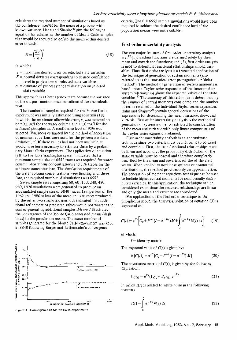
Seven sample sets comprising 60,60, 120, 240,480, 960, 1920 simulations were generated to produce an accumulated sample size of 3840 traces. Comparison of the 1962 and 1980 values of the mean and variances produced by the other two stochastic methods indicated that additional refinement of predicted values would not warrant the cost of generating additional samples. Figure I illustrates the convergence of the Monte Carlo generated means (dash lines) to the population means. The exact number of samples generated for the Monte Carlo experiment was kept at 3840 following Burges and Lettenmaier’s convergence

criteria. The full 6552 sample simulations would have been required to achieve the desired confidence level if the population means were not available.

First order uncertainty analysis

The two major features of first order uncertainty analysis are:27 (1) random functions are defined solely by their mean and’covariance functions; and (2), first order analysis is used to determine functional relationships among variables. Thus, first order analysis is a truncated application of the technique of generation of system moments (also referred to as the ‘statistical error propagation’ or ‘delta method’). The method of generation of system moments is based upon a Taylor series expansion of the functional or system relationships about the expected values of the state variables.20 The accuracy of this technique is determined by the number of central moments considered and the number of terms retained in the individual Taylor series expansion. Hahn and Shapiro2’ provide general derivations of the expressions for determining the mean, variance, skew, and kurtosis. First order uncertainty analysis is the method of generation of system moments restricted to consideration of the mean and variance with only linear components of the Taylor series expansion retained.

First order uncertainty analysis is an approximate technique since two criteria must be met for it to be exact and complete. First, the true functional relationships must be linear and secondly, the probability distribution of the static variable must be normal and therefore completely described by the mean and covarianceof the of the state vector. When applied to nonlinear systems or nonnormal distributions, the method provides only an approximation. The generation of moment equations technique can be used to include higher central moments for nonnormally distributed variables. In this application, the technique can be considered exact since the assumed relationships are linear and only the mean and variance are considered.

For application of the first order technique to the phosphorus model the analytical solution of equation (3) is expressed as:

t

epFf)M+ emFsW(s) ds 1 (19)

in which:

I = identity matrix

The expected value of C(t) is given by:

E[C(t)] = eFf[Co+ F-‘(I - eCF3 M]

The covariance matrix of C(r), is given by the following expression:

r c(~) = eFf(rc, + rz($ eFTt in which z(t) is related to white noise in the following manner :

t

z(t) = s e - Fs W(s) ds

(21)

figure 7 Convergence of Monte Carlo experiment 0



The covariance matrix of z(t) is given by:

t 1

r z(r) = ss

eeFSQG(s - u) eeFU ds du

00

in which:

(23)

6(s - u) = dirac delta function

In equation (19) is was assumed that the phosphorus loading rate,A4, is independent of time. Therefore, equations (20) and (21) were reinitialized at the beginning of each year simulated to reflect the yearly variations in M.

Comparison of stochastic techniques

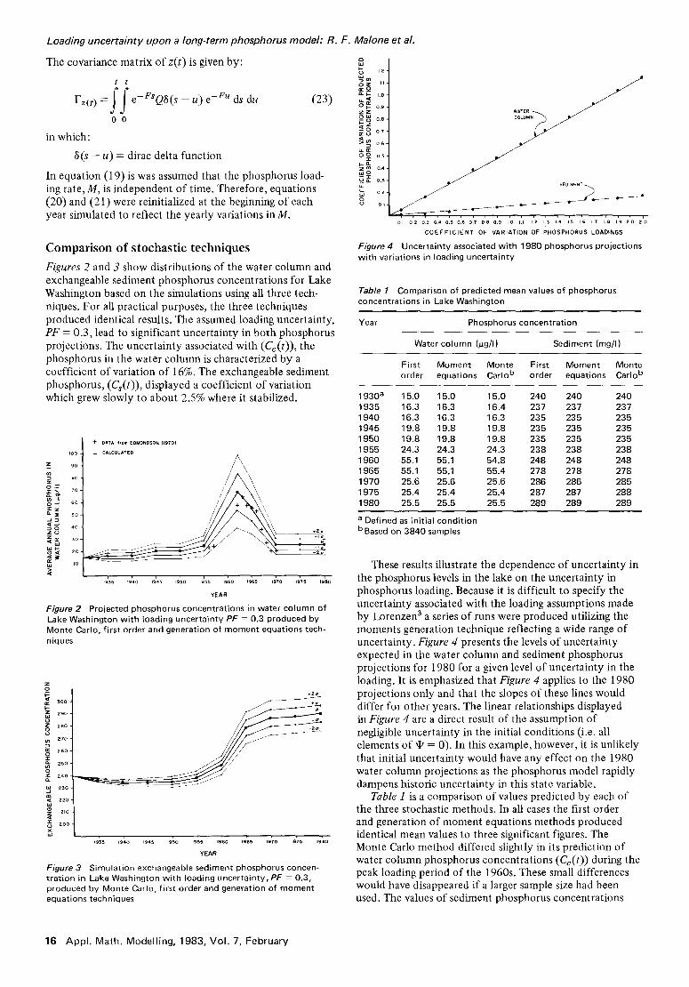
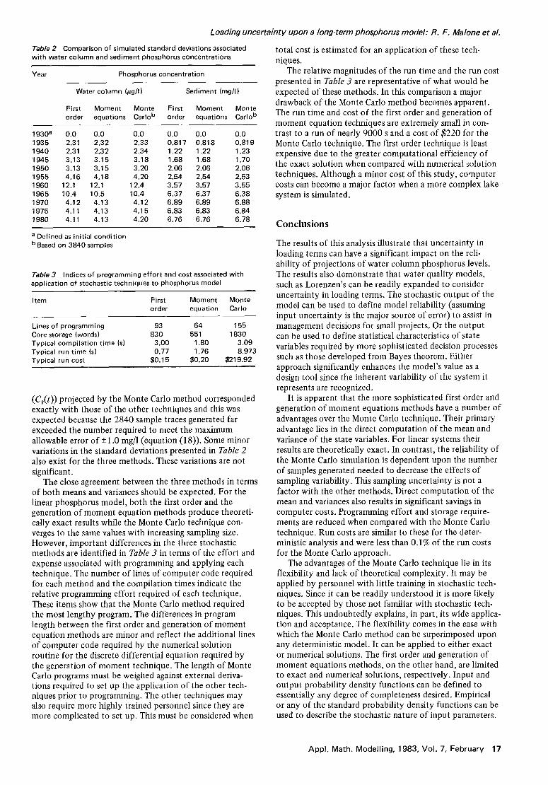
Figures 2 and 3 show distributions of the water column and exchangeable sediment phosphorus concentrations for Lake Washington based on the simulations using all three techniques. For all practical purposes, the three techniques produced identical results. The assumed loading uncertainty, PF = 0.3, lead to significant uncertainty in both phosphorus projections. The uncertainty associated with (Cc(t)), the phosphorus in the water column is characterized by a coefficient of variation of 16%. The exchangeable sediment phosphorus, (Cs(t)), displayed a coefficient of variation which grew slowly to about 2.5% where it stabilized.

YEAR

Figure 2 Projected phosphorus concentrations in water column of Lake Washington with loading uncertainty PF = 0.3 produced by Monte Carlo, first order and generation of moment equations techniques

Figure 3 Simulation exchangeable sediment phosphorus concen. tration in Lake Washington with loading uncertainty, PF = 0.3, produced by Monte Carlo, first order and generation of moment equations techniques

COEFFICIENT OF VARIATION OF PHOSPHORUS LOADINGS

Figure 4 Uncertainty associated with 1980 phosphorus projections

with variations in loading uncertainty

Table 7 Comparison of predicted mean values of phosphorus concentrations in Lake Washington

Year Phosphorus concentration

1930a 1935 1940 1945 1950 1955 1960 1965 1970 1975 1980

Water column (pg/l) Sediment (mg/l)

First Moment Monte First Moment Monte order equations Carlob order equations Carlob

15.0 15.0 15.0 240 240 240 16.3 16.3 16.4 237 237 237 16.3 16.3 16.3 235 235 235 19.8 19.8 19.8 235 235 235 19.8 19.8 19.8 235 235 235 24.3 24.3 24.3 238 238 238 55.1 55.1 54.8 248 248 248 55.1 55.1 55.4 278 278 278 25.6 25.6 25.6 286 286 285 25.4 25.4 25.4 287 287 288 25.5 25.5 25.5 289 289 289

a Defined as initial condition b Based on 3840 samples

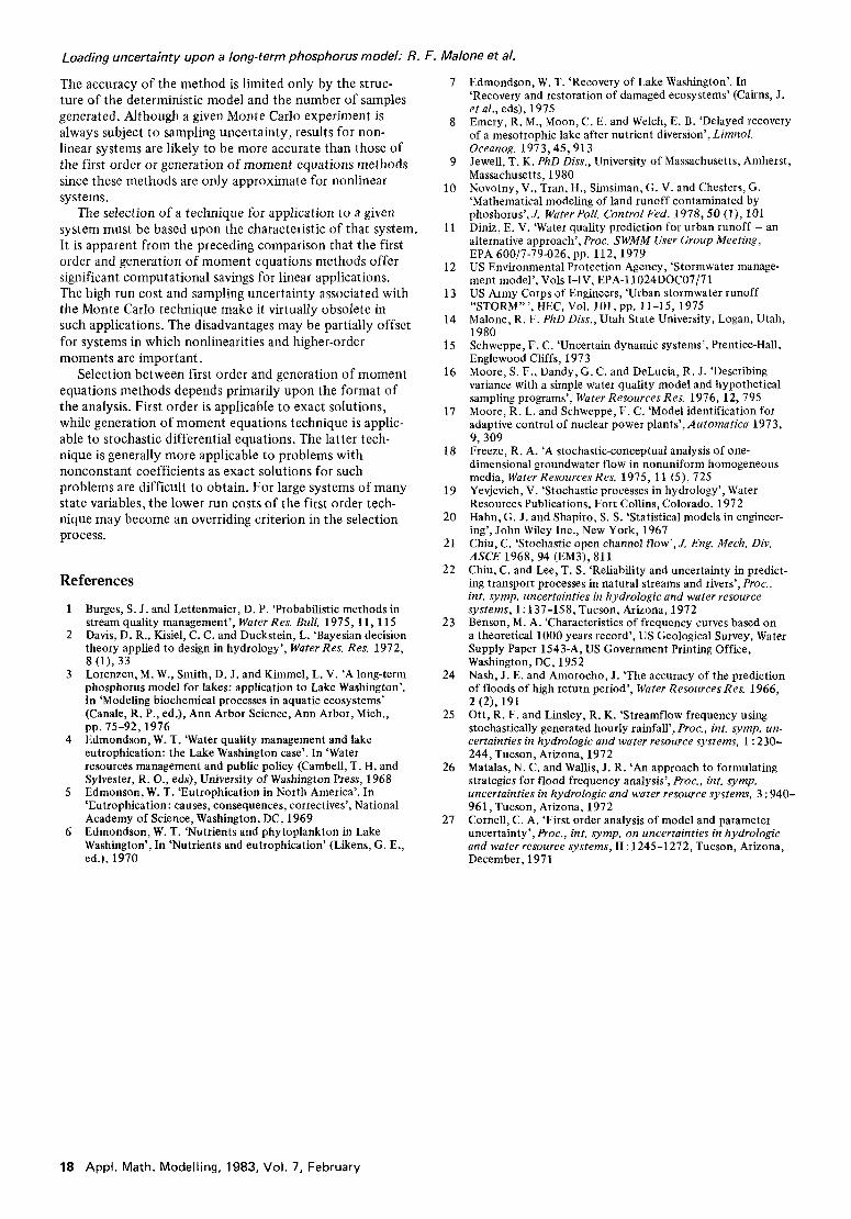
These results illustrate the dependence of uncertainty in the phosphorus levels in the lake on the uncertainty in phosphorus loading. Because it is difficult to specify the uncertainty associated with the loading assumptions made by Lorenzen” a series of runs were produced utilizing the moments generation technique reflecting a wide range of uncertainty. Figure 4 presents the levels of uncertainty expected in the water column and sediment phosphorus projections for 1980 for a given level of uncertainty in the loading. It is emphasized that Figure 4 applies to the 1980 projections only and that the slopes of these lines would differ for other years. The linear relationships displayed in Figure 4 are a direct result of the assumption of negligible uncertainty in the initial conditions (i.e. all elements of \k = 0). In this example, however, it is unlikely that initial uncertainty would have any effect on the 1980 water column projections as the phosphorus model rapidly dampens historic uncertainty in this state variable.

Table I is a comparison of values predicted by each of the three stochastic methods. In all cases the first order and generation of moment equations methods produced identical mean values to three significant figures. The Monte Carlo method differed slightly in its prediction of water column phosphorus concentrations (C=(t)) during the peak loading period of the 1960s. These small differences would have disappeared if a larger sample size had been used. The values of sediment phosphorus concentrations



Tab/e 2 Comparison of simulated standard deviations associated with water column and sediment phosphorus concentrations

Year Phosphorus concentration

Water column (pg/l) Sediment (mg/l)

First Moment Monte First Moment Monte order equations Carlob order equations Carlob

1930e 0.0 0.0 0.0 0.0 0.0 0.0 1935 2.31 2.32 2.33 0.817 0.818 0.819 1940 2.31 2.32 2.34 1.22 1.22 1.23 1945 3.13 3.15 3.18 1.68 1.68 1.70 1950 3.13 3.15 3.20 2.06 2.06 2.06 1955 4.16 4.18 4.20 2.54 2.54 2.53 1960 12.1 12.1 12.4 3.57 3.57 3.55 1965 10.4 10.5 10.4 6.37 6.37 6.38 1970 4.12 4.13 4.12 6.89 6.89 6.88 1975 4.1 1 4.13 4.15 6.83 6.83 6.84 1980 4.11 4.13 4.20 6.76 6.76 6.78

a Defined as initial condition b Based on 3840 samples

Tab/e 3 Indices of programming effort and cost associated with application of stochastic techniques to phosphorus model

Item First order

Moment Monte equation Carlo

Lines of programming 93 64 155 Core storage (words) 830 551 1830 Typical compilation time fs) 3.00 1.80 3.09 Typical run time (s) 0.77 I .76 8.973 Typical run cost $0.15 $0.20 $219.92

(Cs(t)) projected by the Monte Carlo method corresponded exactly with those of the other techniques and this was expected because the 2840 sample traces generated far exceeded the number required to meet the maximum allowable error of + 1 .O mg/l (equation (18)). Some minor variations in the standard deviations presented in Table 2 also exist for the three methods. These variations are not significant.

The close agreement between the three methods in terms of both means and variances should be expected. For the linear phosphorus model, both the first order and the generation of moment equation methods produce theoretically exact results while the Monte Carlo technique converges to the same values with increasing sampling size. However, important differences in the three stochastic methods are identified in Table 3 in terms of the effort and expense associated with programming and applying each technique. The number of lines of computer code required for each method and the compilation times indicate the relative programming effort required of each technique. These items show that the Monte Carlo method required the most lengthy program. The differences in program length between the first order and generation of moment equation methods are minor and reflect the additional lines of computer code required by the numerical solution routine for the discrete differential equation required by the generation of moment technique. The length of Monte Carlo programs must be weighed against external derivations required to set up the application of the other techniques prior to programming. The other techniques may also require more highly trained personnel since they are more complicated to set up. This must be considered when

total cost is estimated for an application of these techniques.

The relative magnitudes of the run time and the run cost presented in Table 3 are representative of what would be expected of these methods. In this comparison a major drawback of the Monte Carlo method becomes apparent. The run time and cost of the first order and generation of moment equation techniques are extremely small in contrast to a run of nearly 9000 s and a cost of $220 for the Monte Carlo technique. The first order technique is least expensive due to the greater computational efficiency of the exact solution when compared with numerical solution techniques. Although a minor cost of this study, computer costs can become a major factor when a more complex lake system is simulated.

Conclusions

The results of this analysis illustrate that uncertainty in loading terms can have a significant impact on the reliability of projections of water column phosphorus levels. The results also demonstrate that water quality models, such as Lorenzen’s can be readily expanded to consider uncertainty in loading terms. The stochastic output of the model can be used to define model reliability (assuming input uncertainty is the major source of error) to assist in management decisions for small projects. Or the output can be used to define statistical characteristics of state variables required by more sophisticated decision processes such as those developed from Bayes theorem. Either approach significantly enhances the model’s value as a design tool since the inherent variability of the system it represents are recognized.

It is apparent that the more sophisticated first order and generation of moment equations methods have a number of advantages over the Monte Carlo technique. Their primary advantage lies in the direct computation of the mean and variance of the state variables. For linear systems their results are theoretically exact. In contrast, the reliability of the Monte Carlo simulation is dependent upon the number of samples generated needed to decrease the effects of sampling variability. This sampling uncertainty is not a factor with the other methods. Direct computation of the mean and variances also results in significant savings in computer costs. Programming effort and storage requirements are reduced when compared with the Monte Carlo technique. Run costs are similar to these for the deterministic analysis and were less than 0.1% of the run costs for the Monte Carlo approach.

The advantages of the Monte Carlo technique lie in its flexibility and lack of theoretical complexity. It may be applied by personnel with little training in stochastic techniques. Since it can be readily understood it is more likely to be accepted by those not familiar with stochastic techniques. This undoubtedly explains, in part, its wide application and acceptance. The flexibility comes in the ease with which the Monte Carlo method can be superimposed upon any deterministic model. It can be applied to either exact or numerical solutions. The first order and generation of moment equations methods, on the other hand, are limited to exact and numerical solutions, respectively. Input and output probability density functions can be defined to essentially any degree of completeness desired. Empirical or any of the standard probability density functions can be used to describe the stochastic nature of input parameters.



The accuracy of the method is limited only by the structure of the deterministic model and the number of samples generated. Although a given Monte Carlo experiment is always subject to sampling uncertainty, results for nonlinear systems are likely to be more accurate than those of the first order or generation of moment equations methods since these methods are only approximate for nonlinear systems.

The selection of a technique for application to a given system must be based upon the characteristic of that system. It is apparent from the preceding comparison that the first order and generation of moment equations methods offer significant computational savings for linear applications. The high run cost and sampling uncertainty associated with the Monte Carlo technique make it virtually obsolete in such applications. The disadvantages may be partially offset for systems in which nonlinearities and higher-order moments are important.

Selection between first order and generation of moment equations methods depends primarily upon the format of the analysis. First order is applicable to exact solutions, while generation of moment equations technique is applicable to stochastic differential equations. The latter technique is generally more applicable to problems with nonconstant coefficients as exact solutions for such problems are difficult to obtain. For large systems of many state variables, the lower run costs of the first order technique may become an overriding criterion in the selection process.

References

Burges, S. J. and Lettenmaier, D. P. ‘Probabilistic methods in stream quality management’, Water Rex Bull. 1975, 11, 115 Davis, D. R., Kisiel, C. C. and Duckstein, L. ‘Bayesian decision theory applied to design in hydrology’, Water Res. Res. 1972, 8 Cl), 33 Lorenzen, M. W., Smith, D. J. and Kimmel, L. V. ‘A long-term phosphorus model for lakes: application to Lake Washington’. In ‘Modeling biochemical processes in aquatic ecosystems’ (Canale, R. P., ed.), Ann Arbor Science, Ann Arbor, Mich., pp. 75-92,1976 Edmondson, W. T. ‘Water quality management and lake eutrophication: the Lake Washington case’. In ‘Water resources management and public policy (Cambell, T. H. and Sylvester, R. O., eds), University of Washington Press, 1968 Edmonson, W. T. ‘Eutrophication in North America’. In ‘Eutrophication: causes, consequences, correctives’, National Academy of Science, Washington, DC, 1969 Edmondson, W. T. ‘Nutrients and phytoplankton in Lake Washington’, In ‘Nutrients and eutrophication’ (Likens, G. E., ed.), 1970

I

8

9

10

11

12

13

14

15

16

17

18

19

20

21

22

23

24

25

26

27

Edmondson, W. T. ‘Recovery of Lake Washington’. In ‘Recovery and restoration of damaged ecosystems’ (Cairns, J. et al., eds), 1975 Emery, R. M., Moon, C. E. and Welch, E. B. ‘Delayed recovery of a mesotrophic lake after nutrient diversion’, Limnol. Oceanog. 1973,45,913 JeweIl, T. K. PhD Diss., University of Massachusetts, Amherst, Massachusetts, 1980 Novotny, V., Tran, H., Simsiman, G. V. and Chesters, G. ‘Mathematical modeling of land runoff contaminated by vhoshorus’. J. WaterPoll. Control Fed. 1978.50 (1). 101 Diniz, E. VI ‘Water quality prediction for urban runoff - an alternative approach’, Proc. SWMM User Group Meeting, EPA 600/7-79-026, pp. 112,1979 US Environmental Protection Agency, ‘Stormwater management model’, Vols I-IV, EPA-l 1024DOC07/7 1 US Army Corps of Engineers, ‘Urban stormwater runoff “STORM”‘, HEC, Vol. 101, pp. 11-15, 1975 Malone, R. F. PhD Diss., Utah State University, Logan, Utah, 1980 Schweppe, F. C. ‘Uncertain dynamic systems’, Prentice-Hall, Englewood Cliffs, 1973 Moore, S. F., Dandy, G. C. and DeLucia, R. J. ‘Describing variance with a simple water quality model and hypothetical sampling programs’, Water Resources Res. 1976, 12,795 Moore, R. L. and Schweppe, F. C. ‘Model identification for adaptive control of nuclear power plants’, htomatica 1973, 9,309 Freeze, R. A. ‘A stochastic-conceptual analysis of one- dimensional groundwater flow in nonuniform homogeneous media, Water ResourcesRes. 1975, 11 (5), 725 Yevjevich, V. ‘Stochastic processes in hydrology’, Water Resources Publications, Fort Collins, Colorado, 1972 Hahn, G. J. and Shapiro, S. S. ‘Statistical models in engineering’, John Wiley Inc., New York, 1967 Chiu, C. ‘Stochastic open channel flow’, J. Eng. Meek. Div. ASCE 1968,94 (EM3), 811 Chiu, C. and Lee, T. S. ‘Reliability and uncertainty in predicting transport processes in natural streams and rivers’, Proc., int. symp. uncertainties in hydrologic and water resource systems, 1: 137-158, Tucson, Arizona, 1972 Benson, M. A. ‘Characteristics of frequency curves based on a theoretical 1000 years record’, US Geological Survey, Water Supply Paper 1543-A, US Government Printing Office, Washington, DC, 195 2 Nash, J. E. and Amorocho, J. ‘The accuracy of the prediction of floods of high return period’, Water Resources Res. 1966, 2 (21,191 Ott, R. F. and Linsley, R. K. ‘Streamflow frequency using stochastically generated hourly rainfall’, Proc., int. symp. uncertainties in hydrologic and water resource systems, 1 : 230- 244, Tucson, Arizona, 1972 Matalas, N. C. and Wallis, J. R. ‘An approach to formulating strategies for flood frequency analysis’, Proc., int. symp. uncertainties in hydrologic and water resource systems, 3 : 940- 961, Tucson, Arizona, 1972 Cornell, C. A. ‘First order analysis of model and parameter uncertainty’,Pfoc., int. symp. on uncertainties in hydrologic and water resource systems, II : 1245-1272, Tucson, Arizona, December, 1971


comparison of techniques for assessing effects of loading uncertainty upon a long term phosphorous...

Documents