comparison of some chemometric tools for metabonomics ... · comparison of some chemometric tools...

Available online at www.sciencedirect.com

ory Systems 91 (2008) 54–66www.elsevier.com/locate/chemolab

Chemometrics and Intelligent Laborat

Comparison of some chemometric tools for metabonomicsbiomarker identification

Réjane Rousseau a,⁎, Bernadette Govaerts a, Michel Verleysen a,b, Bruno Boulanger c

a Université Catholique de Louvain, Institut de Statistique, Voie du Roman Pays 20, B-1348 Louvain-la-Neuve, Belgiumb Université Catholique de Louvain, Machine Learning Group - DICE, Belgium

c Eli Lilly, European Early Phase Statistics, Belgium

Received 29 December 2006; received in revised form 15 June 2007; accepted 22 June 2007Available online 29 June 2007

Abstract

NMR-based metabonomics discovery approaches require statistical methods to extract, from large and complex spectral databases, biomarkers orbiologically significant variables that best represent defined biological conditions. This paper explores the respective effectiveness of six multivariatemethods: multiple hypotheses testing, supervised extensions of principal (PCA) and independent components analysis (ICA), discriminant partialleast squares, linear logistic regression and classification trees. Each method has been adapted in order to provide a biomarker score for each zone ofthe spectrum. These scores aim at giving to the biologist indications on which metabolites of the analyzed biofluid are potentially affected by astressor factor of interest (e.g. toxicity of a drug, presence of a given disease or therapeutic effect of a drug). The applications of the six methods tosamples of 60 and 200 spectra issued from a semi-artificial database allowed to evaluate their respective properties. In particular, their sensitivities andfalse discovery rates (FDR) are illustrated through receiver operating characteristics curves (ROC) and the resulting identifications are used to showtheir specificities and relative advantages.The paper recommends to discard two methods for biomarker identification: the PCA showing a generallow efficiency and the CART which is very sensitive to noise. The other 4 methods give promising results, each having its own specificities.© 2007 Elsevier B.V. All rights reserved.

Keywords: Metabonomics; Multivariate statistics; Variable selection; Biomarker identification; 1H NMR spectroscopy

1. Introduction

The recent biological ‘Omics’ domain is formed by severaltechnological platforms (Genomics, Proteomics, Metabonomics)using multiparametric biochemical information derived from thedifferent levels of biomolecular organization (respectively thegenes, proteins andmetabolites) to study the living organisms. Allof these Omics sciences rely on analytical chemistry methods,resulting in complex multivariate datasets which require a largevariety of statistical chemometric and bioinformatic tools forinterpretation. Due to the central place of metabolites in organi-zation of living systems, Metabonomics, the most recenttechnology in the world of “Omics”, is particularly indicated toextract biochemical information reflecting the actual biologicalevents. Genomics and proteomics information describing tran-scriptional effects and protein synthesis do not provide a complete

⁎ Corresponding author. Tel.: +32 10 47 30 49; fax: +32 10 47 30 32.E-mail address: [email protected] (R. Rousseau).

0169-7439/$ - see front matter © 2007 Elsevier B.V. All rights reserved.doi:10.1016/j.chemolab.2007.06.008

description of the perturbation cause by a disease or a xenobioticon an organism. Alternatively, Metabonomics analyses the entirepool of endogenous metabolites in biofluids and creates a biolo-gical summary more complete and also closest to the phenotype.Consequently, the metabonomics approach is a promisingframework to build detection tools of a response of an organismto a stressor.

Metabonomics is formally defined as “The quantitative mea-surement of the dynamic multi-parametric metabolic response ofliving systems to physiological stimuli or genetic modification”[1]. Metabonomics aims to approach the modifications of endo-genous metabolites consecutive to a physiopathological stimu-lus or genetic modification by the combined use of an analyticaltechnology and multivariate statistical methods. Proton nuclearmagnetic resonance (1H NMR) spectroscopy generates spectralprofiles describing the concentration, size and structure of meta-bolites contained in collected biofluid samples. This analyticaltechnology remains the more efficient in metabonomics as theanalysis is non-destructive, non-selective, cost-effective and

mailto:[email protected]

http://dx.doi.org/10.1016/j.chemolab.2007.06.008

55R. Rousseau et al. / Chemometrics and Intelligent Laboratory Systems 91 (2008) 54–66

typically takes only a few minutes per sample requiring little or nosample pretreatment or reagent. Each resulting spectrum offers anoverview of the metabolic state of the organism at the moment ofthe biofluid sampling. However, stressors from different categoriesaffecting the organism will alter the concentration of the meta-bolites and consequently modify the spectral profile. On this basis,comparison of spectra in various specific states allows to detectalterations corresponding to biochemical changes inherent to thepresence of a stressor. These resulting changes can be mapped bybiologists to known pathways and to quickly build biochemicalhypotheses. Anyway, the principal opportunity provided by thespectra of biofluids is the development of detection tools for thebiological response to a stressor: viewing the recordered spectralchanges as fingerprints of the reaction, the concerned regions of thespectrum can be employed on a new spectral profile to declare ifthis new observation develops the reaction.

However a typical 1H NMR metabonomics study generatesnumerous biofluid samples and related complex 1HNMR spectra,making impossible, even for a trained NMR-spectroscopist, toreveal all the changes by a visual inspection. Moreover, sys-tematic differences between spectra are often hidden in biologicalnoise. Adequate data pre-treatment and reduction tools andchemometric methodologies are then required to extract typicaldifferences between spectra obtained in various states. In this aim,each spectrum domain is first transformed in a set of regionscalled descriptors corresponding each to the summed intensitybelow the spectrum in its region. The observed values of allspectra give rise to a multivariate 1H NMR database, typicallycharacterized by a large number of variables (the descriptors).Multivariate statistical methodologies are then applied to minetypical differences between spectral data in different conditions.

Although the application of metabonomics as detection toolswas first developed in the pharmaceutical industry field for toxicitypredictions and screening, recently applications have expanded theuse of metabonomics to a large variety of domains of lifessciences.Metabonomics is becoming a promising tools for clinicaldiagnosis, as well as environmental security applications [2].

Biomarkers and predictive models are the two different de-tection tools issued from the use of statistical methodologies on1H NMR metabonomics data. A 1H NMR metabonomics bio-marker is defined as a stable change in a 1H NMR spectral regionassociated to the alteration of an endogenous metabolite in re-action to the contact with the considered stressor. Alteration ofthese regions or descriptor(s) serves in research as an indicator ofthe development of a response of the organism to the stressor. Onthe other hand, predictive model are useful in research to providethe probability of the development of this response. Predictivemodel quantitatively characterizes for each spectral region itspertinence to contribute to an adequate description of the presenceof a response of the organism. Biologists then use this quantitativeinformation in order to build a model aimed at validating thepresence of reaction of the organism to a new stressor.

The metabonomics biomarkers, used in research by biologists,are developped or identified beforehand in an experimental 1HNMR database with chemometric analysis. The goal of themethods is to find, in the range covered by the 1H NMR spectrum,the area(s) which is (are) consistently altered by the given factor of

interest (disease, toxicity). Several methods can be considered inorder to identify in multivariate data the more altered variables inpresence of a chosen characteristic [3]. Usually, unsupervisedmethods (Principal component analysis, Hierarchical clusteranalysis, Nonlinear mapping) constitute a first step in metabo-nomics data analysis. Without assuming any previous knowledgeof sample class, these methods enable the visualization of the datain a reduced dimensional space built on the dissimilarities betweensamples with respect to their biochemical composition. In this step,biomarkers are identified in a pertinent space of reduced dimension.For this purpose, principal component analysis (PCA) has beenextensively used in metabonomics litterature. Despite apparentsatisfying published results, the known large sensitivity of PCA tonoise can suggest that improvements are expectedwithmore robustmethods to identify biomarkers in noisy data. Moreover, thetraditional use of PCA remains highly questionable: biomarkers areidentified from the loadings of the two first principal components,while the two first components do not necessarily contain the mostrelevant variations between altered and normal spectra. Sometimes,the results of the initial unsupervised analysis are confirmed by asecond supervised analysis. This one employs classificationmethods as Partial Least Squares (PLS), SIMCA and neuralnetworks, allowing first to separate normal and altered spectra, andsecondly to identify more robust biomarkers [2].

This paper aims in investigating the relatives properties ofadvanced statistical methods for the identification of biomarkersfrom 1HNMR data. As the performances of the PCA usual tool arequestionable, the choice of an appropriate method stays a opendomain. All methods covered in this paper are published toolsselected for their frequent uses in statistics or chemometrics.Nevertheless, some of them are extended in order to fit with thebiomarker identification goal. Some of the methods are used solelyfor identification, others may be used as predictive models too.All are compared based on both qualitative and quantitativeconsiderations.

This paper is organized as follows. Section 2 presents sixpossible methods to identify biomarkers. The first one (MHT) isbased on traditional descriptor-wise multiple hypothesis testing.The next two (s-PCA and s-ICA) are extensions of correspondingtraditional multivariate data reduction tools. The final threemethods (PLS, linear logistic regression and CARTclassificationtrees) provide predictive models from which biomarkers can beextracted. The next sections are devoted to the illustration andcomparison of these methods. Section 3 presents a semi-artificialmetabonomic data base built for this purpose. Section 4 illustratesthe methods on one data set and emphasizes their particularcharacteristics. Finally, Section 5 tests systematically the sixmethods on several data samples and compare their performancesin terms of various criteria as sensitivity, specificity and stability.This comparison will show that all methods, except s-PCA andCART, give promising results. Each of these has its own ad-vantages and provides specific information.

2. Methods

In this section, six methods envisaged for biomarker iden-tification and/or prediction are described, after the presentation

56 R. Rousseau et al. / Chemometrics and Intelligent Laboratory Systems 91 (2008) 54–66

of unified notations. All methods are described both in anintuitive way and an algorithmic form.

Let X be an n×m matrix of spectral data containing n spec-tra, each of them being described by m descriptors. A binaryvector Y of size n identifies the class of each of the n spectra; n0are normal spectra (y=0) and n1 (y=1) are altered ones. Section3 will detail the difference between normal and altered spectra.

The goal here is to find among the m descriptors of thespectrum those which are associated to the concept of classmembership, i.e. those which show systematic differences be-tween the normal and altered classes. Each method provides so-called “biomarker scores” for all spectral descriptors in a vectorb of size m×1. The descriptors with the highest scores will beconsidered as potential biomarkers. The number mb of potentialbiomarkers of interest is chosen either by the biologist orrecommended based on statistical criterion included in themethod.

2.1. Multiple hypothesis testing (MHT)

2.1.1. PresentationIn the emerging-omics techniques, multiple hypothesis

testing (MHT) has become a very popular technique todetermine simultaneously if some descriptors, of a large set ofpossible ones, are altered by a (biological) factor of interest.Micro-array data analysis has been the privileged area ofapplication of such methods. MHT consists in calculating,for each descriptor, a test statistic measuring the effect of thefactor of interest; in our case, this factor is Y, the altered andnormal spectral class identifier. The multiple test procedureaims then at giving a rule to decide which of the calculatedstatistics are statistically significant in controlling the total errorrate of the test. When the number of tests is very high, the falsediscovery rate (FDR), i.e. the number of false discoveries overthe number of discoveries, is usually taken as the error factor tobe controlled. Several methods have been developed in aattempt to control the FDR under independent or dependenthypotheses [4–7]. In this paper, MHT is applied in two steps.First, for each descriptor, a classical t statistic is calculatedto compare the mean spectral intensities of the two groups. Thep-values attached to each statistic are then calculated and trans-formed to build biomarker scores. The Benjamini and Yekutieli[4] rule for multiple testing under dependency is then appliedto set up a cut point between significant descriptors and non-significant ones.

2.1.2. Algorithm

• From the spectral matrix X, calculate, for each descriptorj=1,…, m, the following t statistic:

tj ¼x̄1j � x̄0jffiffiffiffiffiffiffiffiffiffiffiffiffiffi

S21jn1þ S20j

n0

r where x̄kj ¼ 1nk

Xfi:Yi¼kg

Xij and

S2kj ¼1

nk

Xfi:Yi¼kg

ðXij � x̄kjÞ2ð1Þ

• Calculate the individual p-values attached to these t statisticsas

pj ¼ 2PðtvjNjtjjÞ

where tvj is a Student t random variable with vj degrees offreedom. vj is defined by the Welch formula as the closest

integer to

S21n1þS2

0n0

� �2

S41

n21ðn1�1Þþ

S40

n20ðn0�1Þ

� �

• Define the vector of signed biomarquer scores b=(b1, b2,…,bm) from the following transformation of the pj's:

bj ¼ signðtjÞðlogð1=pjÞÞ

• Choice as potential biomarkers the mb descriptors withthe highest bj's. mb can be chosen by the analyst or bythe Benjamini–Yekutieli FDR controlling rule [4]: mb ¼max i : piV ia

mPn

i¼11i

� �where α is the maximum expected

FDR desired for the multiple testing procedure.

2.2. Supervised principal component analysis (s-PCA)

2.2.1. PresentationIn metabonomics and 1H NMR data exploration, the Prin-

cipal Component Analysis (PCA) [8] is the most commonlyused method by practitioners. However, as discussed above, thetraditional use of PCA in metabonomics remains questionnable,notably due to the use of the two first principal components. AsPCA is here presented as a reference tool for biomarker iden-tification, some improvements are suggested through a methodcalled s-PCA.

s-PCA is performed as follows. A PCA is first applied to thematrix of centered by columns spectra Xc. The normalized scorematrix is then used to find the two components which dis-criminate best between the two groups. This is an unusual, buteffective way of using PCA. Indeed, PCA is an unsupervisedmethod: the principal components are computed without takingthe class information into account. The two first directions,which are usually selected, are therefore not necessarily thosethat maximize the discrimination. Here all directions are firstcomputed, and only the two ones that discriminate the most theclasses are kept. Then, in the plane defined by these two prin-cipal components, the direction that maximizes the discrimina-tion is calculated and the corresponding loadings are chosen asbiomarker scores.

2.2.2. Algorithm

• Center X by columns: X c=X−1n · X̄T where X̄ is the m×1vector of column means and 1n a n×1 vector of ones.

• Perform a PCA on Xc:X c=TPTwhere T is the n×k matrix ofscores and P is the m×k matrix of loadings (k=min(n, m)).

• Normalise the score matrix as C=TΓ − 1/2

where Γ is thediagonal matrix with k eigenvalues.


• By applying formulae (1) to C (instead of X), calculate tstatistics to compare, for each principal component, the nor-malized scores of both groups.

• Search the two components j1 and j2 that maximize ∣tj∣, i.e.which discriminate the best between the two groups.

• In the space of the j1 and j2 components, find the directionwhich maximizes the distance between the two groups cen-troïds and evaluate the contribution of loadings to this di-rection: p⁎ ¼ pj1 c̄1j1 � pj0 c̄0j2 where c̄1j1 is the coordinate onj1 of the mean c̄ 1 of spectra scores from class 1 and c̄0j1 isdefined in the same way.

• Define the biomarkers scores as b=p⁎

• Choose a predefined number of descriptors with highest(absolute) scores as candidate biomarkers.

2.3. Supervised independent component analysis (s-ICA)

2.3.1. PresentationIndependent component analysis (ICA) [9] is methods that

originally aimed in recovering unobserved signals or sourcesfrom linear mixtures of them. In the context of metabonomics1H NMR data, the media analyzed (e.g. plasma, urine) can beseen as a mixture of individual metabolites and NMR spectramay then be interpreted as weighted sums of NMR spectra ofthese single metabolites. If the matrix X of 1H NMR spectra isrich enough, the application of ICA to 1H NMR data shouldthen ideally recover source products included in the analyzedmedia, in particular those that are biomarkers of the causalfactor of interest in the study.

ICA is applied in this context as follows. First ICA is appliedto the matrix of spectra. t statistics are then calculated from themixing coefficients and used to identify sources that are able todiscriminate the two groups of interest. Identified sources canideally be interpreted as spectra of pure or complex metaboliteswhose quantities have been altered by the factor of interest.Mean NMR spectra for both altered and normal group are thenreconstructed from the identified sources and the differencebetween these mean spectra are used as biomarker scores.

2.3.2. Algorithm

• Center X by lines and transpose it: XTc=XT−1m· X̃Twhere X̃is the vector of lines (spectra) means.

• Apply ICA to XTc. e.g. the fastICA algorithm with parallelextraction of components proceeds in three steps:– Reduce by PCA the m×n matrix XTc to a m×k matrix ofscores T (k≤min(n, m)): XT c=TPT+E where E is theerror.

– Apply ICA to T: T=WS where S is the m×k matrix ofsources and W is the k×k unmixing matrix.

– Derive the mixing matrix A such that XT c=SA.• Search for the sources that discriminate the most normal andaltered spectra.– Calculate t statistics to compare, for each source, themixing coefficients in both groups. The t statistics arederived by applying formulae (1) to AT, the transposedmixing matrix.

– Choose the k⁎ sources with the highest tj as those thatdiscriminate the most the two groups. k⁎ can be choseneither visually or with a FDR based method applied onthe tj's.

– Build S⁎ and A⁎ the subset matrices of S and A corres-ponding to these k⁎ sources.

• Calculate the biomarker scores as b=S⁎ A⁎ Z where Z is a(n×1) vector with Zi=−1/n0 if Yi=0 and 1/n1 otherwise.

• Choose a predefined number of descriptors with highest(absolute) scores as candidate biomarkers.

2.4. Discriminant Partial Least Squares (PLS-DA)

2.4.1. PresentationPartial least squares discriminant analysis (PLS-DA) [10,11]

is a partial least squares regression aimed at predicting one(or several) binary responses(s) Y from a set X of descriptors.PLS-DA implements a compromise between the usual dis-criminant analysis and a discriminant analysis on the sig-nificant principal components of the descriptor variables. It isspecifically suited to deal with problems where the number ofpredictors is large (compared to the number of observations)and collinear, two major challenges encountered with 1H NMRdata.

This paper suggests to apply PLS-DA for biomarker iden-tification as follows. First, a PLS-DA prediction model is esti-mated [12]; the number of significant components is then chosenaccording to a cross-validation based criterion. The model pro-vides regression parameters that can be used as biomarker scoresb. The descriptors with the highest (absolute) coefficients arecandidate biomarkers.

2.4.2. Algorithm

• Center X by columns : X c=X−1n · X̄T.• Choose the optimal number of components of the PLSmodel using an adequate validation technique and criterion.The RMSEP (Root mean square error of prediction) [13] isa traditional criterion used in this context. It can be cal-culated for each size of model on an external validationset or, when no validation set is available, by k-foldcross-validation.

• Build the PLS regression prediction equation Ŷ=X cb usingthe previously chosen number of components.

• Define b as the vector of biomarker scores.• Choose a predefined number of descriptors with highest(absolute) scores as candidate biomarkers.

2.5. Linear logistic regression (LLR)

2.5.1. PresentationLinear logistic regression (LLR) [14] generalises classical

multiple regression to binary responses. It aims at predicting theprobability of class membership π=P (Y=1) as a function of aset of exploratory variables x=(x1, x2,…, xk)′. In order to get amodel response in the [0, 1] interval, the π is transformed withthe logistic transformation: g ¼ log p

1�p

and η is expressed as


a linear combination of x as η=α+δ′x. The parameters areestimated by maximum likelihood to take into account theBernouilli distribution of the response Y.

Several points must be discussed when applying LLR tobiomarker identification. As the number of potential regressors(descriptors) m is high and, in most cases, larger than thenumber of spectra (n≪m), a dimension reduction or variableselection technique must be first applied to allow model esti-mation. Variable selection is privileged in this paper because thevariables (descriptors) selected in the model can directly be seenas potential biomarkers. Forward selection (a technique thatadds descriptors and never deletes them) and stepwise-forward(which starts with an empty set and adds or removes a singlepredictor variable at each step of the procedure) have beentested. Forward selection has demonstrated to be adequate inthis context. The Akaike AIC criterion [15] is commonly usedto select the variables to be entered into the model. The AICcriterion is defined as AIC=−2log(L)+2(k+1) where L is thelikelihood of the estimated model, and k is the number ofvariable included. When a model has been set up, biomarkersscores may be derived from the p-values of the regressioncoefficients.

2.5.2. Algorithm

• Estimate a model with the constant term only and calculatethe corresponding AIC.

• Repeat for k=1,…, mb:– Try to enter each descriptor xj (j=1,…, m) as a supple-mentary variable in the model and calculate the corres-ponding AICj;

– enter in the model variable xj such that AICj is minimum.• Stop either when a predefined maximum number mb ofdescriptor is reached or when the AIC criterion can not bedecreased any more.

• Take as biomarker scores bj=0 if descriptor j is not chosenin the model and bj=sign(δ̂j)(1/pj) for the other descriptors.pj is the p-value of the Wald test on the regression para-meter δj.

2.6. Classification and regression trees (CART)

2.6.1. PresentationThe CART tree classifier [16] implements a strategy where a

complex problem is divided into simplest sub-problems, withthe advantage that it becomes possible to follow the classifi-cation process through each node of the decision tree. In thecontext of this paper, CART is proposed to realise recursive anditerative binary segmentations of the descriptor space in orderto direct spectra to smaller and smaller groups that are moreand more homogeneous with regards to the class. Whenlooking for biomarkers, the tree is not developed for itscapacity to predict the class membership but for its stepwiseselection of a subset of features relevant for class discrimina-tion: the construction of the tree highlights in segmentationrules the descriptors with a good discriminant power betweenthe two classes of spectra.

2.6.2. Algorithm

• Build the maximal tree model Tmax by repeating segmenta-tion until the number of spectra in each subgroup is less orequal than 5 as suggested by Breinman ([16] p82):– Define a binary segmentation rule by a descriptor xj andits threshold xj

(t) chosen as to maximise the decrease of theGini impurety criterion ([16] p38);

– based on the value of xij, direct each spectrum i of thenode to the left or the right child-node according to thechosen segmentation rule (xij≤orNxj

(t)).• If a fixed mb is required, take as biomarkers the descriptorsxj's corresponding to the mb segmentation rules with thehighest number of spectra in the branch under the corres-ponding node. The biomarker score bj is this number whenxj is in this biomarker list and 0 otherwise. Note that thenumber of segmentation rules in the tree may be smallerthan mb.

• If one want to choose automatically the number of bio-markers mb, the tree Tmax may be reduced to a smaller (andoptimal) tree Topt by cost-complexity pruning [17]. Thismethod cuts stepwise the branches of the initial tree whichminimise the increase of error rate. In this sequence of nestedtrees, the optimal one is chosen with respect to its predictiveaccuracy (measured by a deviance) on an external data set ork-fold cross-validation ones.

2.7. Implementation

All algorithms have been implemented in the R language.Links to the used libraries are available on www.cran.r-project.org/src/contrib/Descriptions/. The following libraries were used:for PCA, the pcurve library, for ICA: the fastICA library, forPLS-DA: the pls-pcr library, for LLR: the Design library, forCART: the tree library. TheMHTmethod has been implementedspecifically for this study.

3. Description of the data

3.1. Typical metabonomics data

A typical experimental database is formed by three sets ofdata: a design, a set of 1H NMR spectra and biological and/orhysto-pathological data. The design describes the experimentalconditions underlying each available spectrum. Typical designfactors are: subject (animal or human) ID and characteristics,treatment, dose, time of prelevement. The 1H NMR datasetcontains the spectral evaluations of biofluid samples collectedaccording to the design. After spectra are accumulated, a pri-mary data reduction (“binning”) is carried out by digitizing theone-dimensional spectrum into a series of 250 to 3000 inte-grated regions or descriptor variables. However, a typical me-tabonomics study involves about 30 to 200 spectra or samplemeasurements. The resulting dataset is thus typically charac-terized by a larger number m of variables than the number n ofobservations. Another important characteristic of 1H NMR datais the strong association (dependency) existing between some

http://www.cran.r-project.org/src/contrib/Descriptions/

http://www.cran.r-project.org/src/contrib/Descriptions/

Fig. 1. (a) Typical rat urine NMR spectrum, (b) positions and mean amplitude ofalterations added to urine spectra.


descriptors, due to the fact each molecule can have more thanone spectral peak and hence contribute to a lot more than onedescriptor. As a large variety of dynamic biological systems andprocesses are reflected in spectra, a range of physiologicalconditions, as for example the nutritional status, can also modi-fy spectra. Noise or biological fluctuation are thus natural in thespectral data. Each spectrum of the 1H NMR dataset is alsousually linked to one or more variable(s) aimed at confirming byan independent measure the presence of a response of theorganism towards the stressor. This confirmation is obtained bymeans of the current gold-standard examinations (biologicalmeasures or hysto-pathological ones) generated for the subjectfrom which the spectrum is measured.

3.2. Construction of a semi-artificial database

To explore the capabilities of multivariate statistical methodsto identify biomarkers, a semi-artificial database was built inwhich the descriptors to be identified by the methods are con-trolled. Knowing the biomarkers to be found offers the ad-vantage to evaluate important characteristics of a method as thesensitivity and the specificity of a method. The principles of thisconstruction lays on the addition of random artificial alterationsto normal or placebo real rat urine spectra. By convention, thispaper uses the terms “biomarkers” and “identifications” to makea distinction between respectively the “real alterations that wewant to detect” and “the results or selection of descriptorsindicated by the method as biomarker”.

3.2.1. Placebo dataThe placebo data are composed of more than 800 spectra

supposed to reflect a situation of physiological stability in raturine. Each of them is issued from the COMET [18] databaseand corresponds to the spectral profile obtained from a “control”rat (which did not receive any treatment). All spectra weremeasured at a 1H NMR frequency of 600 MHZ at the ImperialCollege London, using a flow injection process.

After acquisition, spectral FID signals were automaticallytreated and converted to variables using a Matlab library(BUBBLE) developed at Eli Lilly [19]. Bubble automaticallyperformed, in sequence, suppression of the water resonance, anapodisation, a baseline correction, a warping to align shiftedpeaks. To decrease the inter-sample variability, a normalizationis also realized, dividing each spectra by the median of a wellchosen part of spectral descriptors. The last step reduces, bysimple integration, the part of the spectrum between 0.2 and10 ppm to 500 descriptors. Finally, some statistical tools (eucli-dian and Mahalanobis distances and PCA) were used to findoutliers in the set of spectra and some of them were removed(less than 20). A typical urine spectra coming out of this processis given in Fig. 1a.

3.2.2. Simulation of alterationsAmong the 500 descriptors, 46 were chosen to become

biomarkers. These 46 descriptors were, for half of the spectra inthe database, altered according to the description below, in orderto simulate the response of an organism to a stressor or treat-

ment. The 46 descriptors are chosen in ten consecutive regionsof the spectra as shown in Fig. 1b. Half of these 46 descriptorsand five regions are localized in a first part (index from 140 to180) of the spectra contain a low level of noise; the otherdescriptors and regions are localized in a second part (indexfrom 340 to 380) of the spectra, where the level of noise ishigher. The alterations consist in adding to the placebo spectrarandom draws of Gamma distributions, whose means take theform of 10 peaks with different widths localized in the tenregions. Fig. 1b shows the mean height of these peaks. Thesignal of these alterations represents in average 30 percent of thenoise of the spectra. Note also that four peaks have a width of7 descriptors and the 6 other peaks have a smaller width of3 descriptors, for a total of 46 descriptors or biomarkers.Moreover, some pairs (see arrows in Fig. 1b) of alterations weredesigned to be correlated, by using the same Gamma distri-bution to generate peaks, so that only six independent Gammadistributions have been used instead of 10. This last feature ofthe database makes it possible to test if the biomarker identi-fication methods are able or not to discover correlated bio-markers. The 6 sets of 3 to 14 single descriptors or biomarkersgenerated independently will be called below the “independent”biomarkers. Note finally that each placebo spectrum was onlyaltered with two (randomly chosen) from the six possible inde-pendent biomarkers. This simulates the fact that each organismdoesn’t necessarily respond the same way to a stimulus. Adataset of 400 altered spectra (randomly chosen from the 800placebos) was built with this methodology.

3.3. Construction of the datasets for method testing andcomparison

The dataset available consists therefore in 400 placebospectra and 400 “altered” spectra. The goal of the next sectionsis to show that the methods are able to identify the altereddescriptors. For this purpose, subsamples of size 60 (2×30) and200 (2×100) have been extracted out this dataset to simulatetypical metabonomics sample sizes. In Section 4, one sample of200 spectra was drawn randomly to illustrate the methods. In

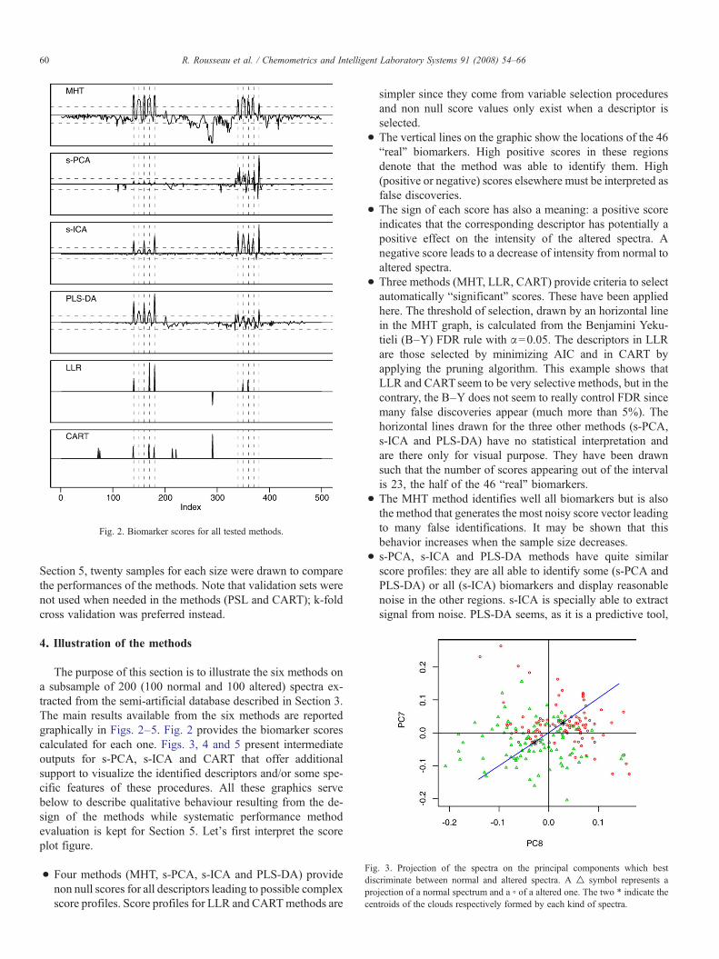
Fig. 2. Biomarker scores for all tested methods.

Fig. 3. Projection of the spectra on the principal components which bestdiscriminate between normal and altered spectra. A △ symbol represents aprojection of a normal spectrum and a ◦ of a altered one. The two ∗ indicate thecentroids of the clouds respectively formed by each kind of spectra.


Section 5, twenty samples for each size were drawn to comparethe performances of the methods. Note that validation sets werenot used when needed in the methods (PSL and CART); k-foldcross validation was preferred instead.

4. Illustration of the methods

The purpose of this section is to illustrate the six methods ona subsample of 200 (100 normal and 100 altered) spectra ex-tracted from the semi-artificial database described in Section 3.The main results available from the six methods are reportedgraphically in Figs. 2–5. Fig. 2 provides the biomarker scorescalculated for each one. Figs. 3, 4 and 5 present intermediateoutputs for s-PCA, s-ICA and CART that offer additionalsupport to visualize the identified descriptors and/or some spe-cific features of these procedures. All these graphics servebelow to describe qualitative behaviour resulting from the de-sign of the methods while systematic performance methodevaluation is kept for Section 5. Let's first interpret the scoreplot figure.

• Four methods (MHT, s-PCA, s-ICA and PLS-DA) providenon null scores for all descriptors leading to possible complexscore profiles. Score profiles for LLR and CARTmethods are

simpler since they come from variable selection proceduresand non null score values only exist when a descriptor isselected.

• The vertical lines on the graphic show the locations of the 46“real” biomarkers. High positive scores in these regionsdenote that the method was able to identify them. High(positive or negative) scores elsewhere must be interpreted asfalse discoveries.

• The sign of each score has also a meaning: a positive scoreindicates that the corresponding descriptor has potentially apositive effect on the intensity of the altered spectra. Anegative score leads to a decrease of intensity from normal toaltered spectra.

• Three methods (MHT, LLR, CART) provide criteria to selectautomatically “significant” scores. These have been appliedhere. The threshold of selection, drawn by an horizontal linein the MHT graph, is calculated from the Benjamini Yeku-tieli (B–Y) FDR rule with α=0.05. The descriptors in LLRare those selected by minimizing AIC and in CART byapplying the pruning algorithm. This example shows thatLLR and CARTseem to be very selective methods, but in thecontrary, the B–Y does not seem to really control FDR sincemany false discoveries appear (much more than 5%). Thehorizontal lines drawn for the three other methods (s-PCA,s-ICA and PLS-DA) have no statistical interpretation andare there only for visual purpose. They have been drawnsuch that the number of scores appearing out of the intervalis 23, the half of the 46 “real” biomarkers.

• The MHT method identifies well all biomarkers but is alsothe method that generates the most noisy score vector leadingto many false identifications. It may be shown that thisbehavior increases when the sample size decreases.

• s-PCA, s-ICA and PLS-DA methods have quite similarscore profiles: they are all able to identify some (s-PCA andPLS-DA) or all (s-ICA) biomarkers and display reasonablenoise in the other regions. s-ICA is specially able to extractsignal from noise. PLS-DA seems, as it is a predictive tool,

Fig. 4. The 10 ICA sources which best discriminate between normal and altered spectra.


to privilege biomarkers from the less noisy spectral region.More curiously, s-PCA performs better in the noisy bio-marker region. This may be due to the fact that the t statisticprivileges high signal even in a noisy area of the spectrum.

• For LLR and CART methods, one can observe that truediscoveries are all coming from independent biomarkers.When one descriptor from an independent biomarker isselected by the procedure, all others are discarded because

Fig. 5. Classification tree before and after pruning. H

they constitute redundant (and correlated) information. Thisbehavior is typical in a forward regression selection tech-nique and in decision trees. Fig. 2 shows that LLR identifies5 (of the 6) independent biomarkers with a little sensitivity tonoise while CART identifies only the three in the first part ofthe spectra. The CART method presents indeed a highsensitivity to noise, as illustrated by the lack of identificationof biomarkers in the second (noisy) part of the spectra. Many

orizontal bars indicate where the tree is pruned.


other simulations have confirmed that basic CART can beefficient in situations without or with low noise but is notable to find signal in presence of higher noise.

The following comments can be made from Figs. 3, 4, and 5:

• Fig. 3 presents, for s-PCA, the projection of the 200 spectrain the space of the two principal components which dis-criminate best normal and altered spectra. This graphicis certainly helpful for most biologists very used to PCAmethods. It shows how well spectra are separated andcan detect outliers. Note that, in this example, the two bestcomponents are the 8th and the 7th. Biologists used to workwith first components should then figure out that high

Fig. 6. Proportions of occurrences of true (positive bars) and fa

variance explained does not mean high discrimination as theclassification factor is not taken into account in a PCA. Moreprecisely, the space of the 7th and 8th components explainsan amount of variance smaller than the space formed by thePC1 and PC2 (7.9% with respect to 14,8%). However,components 7 and 8 contain the part of the variance that isinformative for the identification of biomarkers, as illustratedby the distinction between the two kinds of spectra in Fig. 3.

• Among the 100 estimated sources in s-ICA, 10 independentsources were selected (by a FDR based procedure applied tothe t statistics) to be significantly discriminant. Each of theseindependent sources is illustrated in Fig. 4. The graphic isimpressive: sources S1, S2, S3, S4, S7 and S8 correspondnearly perfectly to the 6 independent biomarkers added to

lse (negative bars) biomarker identification in simulations.


highly variable urine spectra in the artificial database. ICA istherefore able to extract these independent multi-descriptorbiomarkers without prior information on their number andcharacteristics. The “purity” of the sources (especially S1, S2and S7) must also be highlight: the signal can really beextracted from the noise. Sources S5, S6, S9 and S10 areunfortunately less useful: these represent correct biomarkersbut are only parts of the multi-peak independent biomarkers.They are then redundant and it is difficult to explain whythey appear as independent sources. Note that the authorsrealized similar graphics with the loadings of the principalcomponents calculated from s-PCA or PLS-DA. They arenot shown here because they do not reveal any useful infor-mation about independent biomarkers and are much morenoisy.

• Cart tree representation shown in Fig. 5 presents the se-quence of descriptors issued from the recursive segmenta-tion, providing supplementary information on the order ofdescriptor selection and the exact segmentation rules. Thehorizontal line shows where the tree was cut by the pruningalgorithm.

5. Method comparison

The six methods described in this paper have beenillustrated using a single dataset in Section 4. The presentsection compares their performances on several datasets ofdifferent sample sizes. For this purpose, 20 samples of 200spectra (100 altered and 100 placebo ones) and of 60 spectra(30 altered and 30 placebo ones) were drawn at random fromthe semi-artificial database described in Section 3. The 6methods were then applied to each of these 40 datasets.Different samples sizes are used to test the robustness of themethods to small (but realistic in real-life situations) samples.In addition, generating 20 samples eliminates possible effectsof a particular draw while the variability of the results can alsobe studied too.

5.1. Number of identifications

The first results concern the identifications obtained fromeach method. Fig. 6 provides for the 200 spectra and for eachmethod, the proportion of simulations where each descriptor hasbeen identified as a biomarker. The positive bars represent thecorrect identifications; the negative bars indicate false discov-eries. Results for the 60 spectra databases are not given becausethey are very similar and only accentuate the observationscoming out of Fig. 6.

For three methods (s-PCA, s-ICA and PLS-DA), the numberof descriptors mb that the method identifies as biomarkers has tobe fixed by the analyst. As a method can be supposed to have alimited number of correct detections, the number mb for thesemethods has been fixed here at 23, the half of the total 46biomarkers randomly added to the altered spectra. For the threeother algorithms (MHT, LLR and CART), the number of iden-tifications mb is chosen automatically by a statistical criteria asdetailed in Section 2.

These results will be interpreted together with the ROCcurves after the next subsection.

5.2. ROC curves

As the performances of a method strongly depend on thetotal number of identifications mb (both false identifications andbiomarkers correctly identified), it is sometimes difficult tocompare several methods which do not deliver the same numberof identifications. The receiver operating characteristic curve(ROC [20]) provides a way to visualize the performances of amethod for a whole range of possible mbs. It must be noticedthat in the presented ROC curves the performances evolveaccording an experimental condition (the value of mb) and notaccording to a parameter of the method as in the traditionalROC curves. Consequently, the ROC curves shown in thispaper can be non-monotonic. More precisely, it gives for eachnumber mb of identifications, in a chosen range, the methodsensitivity and FDR (false discovery rate). The sensitivity isdefined as the proportion of biomarkers correctly identified(among all biomarkers); the FDR is the percentage of falseidentifications (among all the mb identifications).

As explained in Section 3, there are only 6 independent(multiple) biomarkers among the 46 ones. The sensitivity maythus be defined with respect to the proportion of correct iden-tifications among the 46 biomarkers, or with respect to theproportion of correct identifications found among the 6 inde-pendent ones. These two definitions of sensitivity (thereforeof ROC curves) give the four diagrams of Fig. 7, two for the200 spectra case and two for the 60 spectra one. One curverepresents the mean of the 20 ROC curves obtained from theapplication of one method to the 20 datasets. Each curve pre-sents a method performance in a range of 1 to 46 number ofidentifications.

Good methods are those whose curves are mostly con-centrated in or at least reach the upper left part of the ROCdiagrams.

5.3. Discussion

The following comments can be made from Figs. 6 and 7.The MHT method, with its FDR based threshold criterion,

selects the higher number of descriptors as potential biomarkers(75 in average for the 200 spectra case). It is thus natural thatthis method has a high sensitivity, but this is at the price of ahigh FDR. This confirms the poor performance of the B–Ydecision rule in this context. The MHT t scores are able todiscover biomarkers in both low and high noise region of thespectra but loose clearly its performance in small sample. TheMHT method has also the tendency to make false discoveriesin the nosier part of the spectra. The main advantage of MHT isthen certainly its simplicity coupled with overall acceptableperformances especially in large samples. However, as othermethods don’t require it, the normality of the present H NMRdata haven't be taken into account. A possible lack ofnormality can then have consequence on the MHT score andits performance.

Fig. 7. Mean ROC curves (sensitivity versus false discovery rate) for the 6 methods. For clarity, curves only show symbols representing even number of identifications.


The s-PCA method, traditionally used in this context, isperforming very poorly. As explained in Section 4, s-PCA onlyprovides correct identifications in the presence of big alterationsin an ideal noisy spectra. This is why in the presented morelikely natural case with biggest biomarkers in a noisy part of thespectra, s-PCA is the second worst method (after CART): evenif the number of biomarkers was chosen adequately (whichwould require a well-defined criterion), an increase of the sen-sitivity would be accompanied by a high FDR.

The ICA method is more natural than methods based onPCA: indeed the independence statistical criterion correspondsto the notion of independent biomarkers, contrarily to the de-correlation as in PCA-based algorithms. This is certainly themain advantage of ICA; the consequence is that the independentbiomarkers can be retrieved and plotted in the form of a spec-trum (see Section 4) and the metabolites playing a role asbiomarker can thus potentially be identified.

Besides this interpretation power, the ICA method also givesgood biomarker identification performances. As it can be seenin Fig. 6, biomarkers are correctly identified even in the noisypart of the spectra. ROC curves go also in the upper left cornersof the diagrams, showing that sensitivity can become high whenincreasing the number of identifications without deterioratingtoo much the FDR. In the case of the search for independentbiomarkers, the method is even more efficient. In terms of the

mean number of biomarkers found, only the PLS-DA methodcan compete with the ICA one.

From Fig. 6, it is however visible that the goodperformances of PLS-DA mostly come from the less-noisyregions of the spectra, while the ICA method is more robust inthe strongly noisy regions. At comparable performances interms of ROC curves, it can be concluded that ICA is morerobust to noise than PLS-DA. The PLS-DA method is howeververy efficient in recovering independent biomarkers (it is theonly method that finds always all of them in the 20 experimentswith 200 spectra).

The LLR method is not adequate to find all biomarkers.Indeed, as a purely prediction tool, it stops selecting potentialbiomarkers once the predictive performances are acceptable.This means that once a biomarker is found, all other ones thatare dependent to the first one will not be identified. Indeed, themethod gives much better performances when looking forindependent biomarkers only. It is the method which reaches thehighest sensitivity with the smaller mean number of identifica-tions (0.8 with 5 identifications). However, from Fig. 6, itappears that in the 20 runs, different biomarkers are selectedamong each set of dependent ones. Building different models(from slightly different samples) can thus lead the biologistto find several biomarkers influenced by a single metabolite,which can be interesting in some cases.

Fig. 8. Standard deviation of FDR (top) or sensitivity (bottom) versus number of identifications for the 6 methods. For clarity, curves only show symbols representingodd number of identifications.


The CART method does not lead to good performances. As apredictive tool, it identifies only independent biomarkers. More-over, CARTonly succeeds to identify independent biomarkers inlow-noise regions. The advantage of the CART method residesin its tree representation that is easily interpretable, but coupledto low performances and to be used in non-noisy problems only,i.e. non realistic situation.

Finally, let us remind that PLS-DA, LLR and CART are theonly predictive methods among the six ones, providing them afurther advantage when prediction is also an objective of thestudy.

5.4. Variability of the results

In addition to the comparison of the mean performances ofthe methods over 20 runs, it is important to characterize thevariability of the results among the runs. A high variability canbe considered as a drawback as it makes results less repeatable,but can also be exploited to extract additional information (asdetailed for instance in the LLR paragraph above).

Fig. 8 shows the standard deviations of the sensitivity and ofthe FDR (top and bottom respectively), in the 200 and 60spectra cases (left and right respectively) among the 20 datasets.As it can be seen, the standard deviation of both the sensitivityand the FDR are high in the MHT and s-PCA methods. In the

MHT case, it even increases in the 60-spectra case, proving alow robustness to small samples. On the other hand, PLS-DAand LLR are the more stable methods, LLR being clearly thewinner in small sample. In the ICA case, the surprising resultthat the variance is higher in the 200-spectra case than in the 60-spectra one comes from the difficulty that the ICA method hasto handle high-dimensional signals [21]. Coupled to the fact thatthe ICA method is more robust to noise than other ones, it canbe concluded that the best situation to use ICA is with noisysmall samples.

6. Conclusions

Metabonomics is emerging as a valuable tool in a number ofbiological applications. Althought, the choice of efficient che-mometric methods for biomarkers identification in 1H NMRbased metabonomic remains an important research topic. Thispaper proposes to revisit the traditionally used PCA method andto explore more advances chemometrics and statistical tools toidentify biomarkers from 1H NMR spectra classified in twogroups according to a stressor factor of interest. Each proposedmethod delivers biomarker scores to indicate which metabolitesof the analyzed biofluid are affected by the stressor factor. Theapplication of each method to samples of 60 and 200 spectraissued from a semi-artificial database has allowed to observe the


following properties: easiness of interpretation of the results,robustness to noise, ability to identify biomarkers. ROC curveshave been used to represent method false discovery rates andsensitivities.

Due to their high sensitivities to noise, the CART and theimproved PCA methods have shown bad performances incomparison to the other methods. They are then not recom-mended in spectral databases where the signal to noise ratioand the number of spectra are low. ROC curves of PLS-DA ands-ICA methods have shown good and competitive biomarkeridentification performances. However, each of them presentsspecific relevant characteristics. The s-ICA method is robust tonoise and more interpretable as it is able to recover independentmetabolites from complex spectra. The PLS-DA method is veryeasy to apply and is efficient in recovering independent bio-markers. As it identifies only independent biomarkers, the LLRmethod can not be directly compared to the others. Neverthe-less, it has shown to be very efficient in the context by providingautomatically the smallest number of identifications for analready satisfying proportion of correct independent biomar-kers. The main advantage of the last tested method, the MHTmethod is its simplicity coupled with overall acceptable per-formances especially in large samples.

This work motivates numerous further developments. First,from the application side, the methods are currently tested bythe authors on real biological 1H NMR databases. Their goal isto ensure that the identifications coming out of the methodscorrespond to metabolites present in the biofluids analyzed.Moreover, they want to verify if the ability of s-ICA to recoverindependent biomarkers can also be observed on real data. Onthe methodological side, the good results of PLS-DA and LLRmotivate to explore the performances of two tools: the PenalizedLogistic Regression [22] and the LLR-PLS [23]. The highsensitivity to noise of CART suggests exploring more robustrelated methods as the Random Forests [24]. Finally, the FDRbased criterion used in MHT must clearly be improved.

Acknowledgements

The authors are grateful to Eli Lilly and the Consortiumfor Metabonomic toxicology, especially Jeanmarie Collet, forproviding data. They also thank Paul Eilers for stimulatingdiscussion.

References

[1] J. Nicholson, J. Connelly, J.C. Lindon, E. Holmes, Metabonomics: ageneric platform for the study of drug toxicity and gene function, NatureReviews Drug Discovery 1 (2002) 153–161.

[2] E. Holmes, H. Antti, Chemometric contributions to the evolution of me-tabonomics: mathematical solutions to characterising and interpretingcomplex biological NMR spectra, Analyst 127 (2002) 1549–1557.

[3] J.C. Lindon, E. Holmes, J. Nicholson, Metabonomics techniques andapplications to pharmaceutical research and development, PharmaceuticalResearch 23 (2006) 1075–1088.

[4] Y. Benjamini, D. Yekutieli, The control of the false discovery rate inmultiple testing under dependency, The Annals of Statistics 29 (2001)1165–1188.

[5] V. Tusher, R. Tibshiriani, G. Chu, Significant analysis of microarrayapplied to the ionising radiation response, PNAS 98 (2001) 5116–5121.

[6] J. Storey, A direct approach to false discovery rates, Journal of the RoyalStatistical Society. Series B 64 (2002) 479–498.

[7] J. Storey, D. Siegmund, Strong control, conservative point estimation, andsimultaneous conservative consistency of false discovery rates: a unifiedapproach, Journal of the Royal Statistical Society. Series B 66 (2004)187–205.

[8] I. Jolliffe, Principal Component Analysis, Springer-Verlag, New York,1986.

[9] A. Hyvärinen, E. Oja, Independent component analysis: algorithms andapplications, Neural Networks 13 (2000) 411–430.

[10] M. Barker, W. Rayens, Partial least squares for discrimination, Journal ofChemometrics 17 (2003) 166–173.

[11] H. Martens, T. Næs, Multivariate Calibration, Wiley, Chichester, UK,1989.

[12] S. de Jong, SIMPLS: an alternative approach to partial least squaresregression, Chemometrics and Intelligent Laboratory Systems 18 (1993)251–253.

[13] B. Mevik, H.R. Cederkvist, Mean squared error of prediction (MSEP)estimates for principal component regression (PCR) and partial leastsquares regression (PLSR), Journal of Chemometrics 18 (2004) 422–429.

[14] D.W. Hosmer, S. Lemeshow, Applied Logistic Regression, Wiley, NewYork, 1989.

[15] H. Akaike, A new look at the statistical model identification, IEEE Tras.Automat. Consr. AC, vol. 19, 1974, pp. 716–723.

[16] L.J. Breiman, R. Friedman, R. Olsen, C. Stone, Classification and Reg-ression Trees, Wadsworth, Pacific Grove, CA, 1984.

[17] F. Esposito, D. Malerba, G. Semeraro, A comparative analysis of methodsfor pruning decision trees, IEEE Transactions on Pattern Analysis andMachine Intelligence 19 (1997) 476–491.

[18] J.C. Lindon, J.K. Nicholson, E. Holmes, H. Antti, M.E. Bollard, H. Keun,O. Beckonert, T.M. Ebbels, M.D. Reily, D. Robertson, G.J. Stevens, P.Luke, A.P. Breau, G.H. Cantor, R.H. Bible, U. Niederhauser, H. Senn, G.Schlotterbeck, U.G. Sidelmann, S.M. Laursen, A. Tymiak, B.D. Car, L.Lehman-McKeeman, J.M. Colet, A. Loukaci, C. Thomas, Contemporaryissues in toxicology the role of metabonomics in toxicology and itsevaluation by the COMET project, Toxicology and Applied Pharmacol-ogy 187 (2003) 137–146.

[19] Vanwinsberghe J. Bubble: development of a matlab tool for automated 1HNMR data processing in metabonomics, Master's thesis, Université deStrasbourg, 2005.

[20] J.P. Egan, Signal Detection Theory and ROC Analysis, Academic Press,New York, 1975.

[21] A. Hyvarinen, J. Karhunen, E. Oja, Independent Component Analysis,Wiley, USA, 2001.

[22] P. Eilers, J. Boer, G. Van Ommen, H. Van Houwelingen, Classification ofmicroarray data with penalized logistic regression, Proceedings of SPIEProgress in Biomedical Optics and Images 4266 (2001) 187–198.

[23] V. Nguyen, D. Rocke, Tumor classification by partial least squares usingmicroarray gene expression data, Bioinformatics 18 (2002) 39–50.

[24] LJ. Breiman, Random forests, Machine Learning 45 (2001) 5–32.

comparison of some chemometric tools for metabonomics ... · comparison of some chemometric tools...

Documents