nmr spectroscopy techniques for application to metabonomics · chapter 3 nmr spectroscopy...
TRANSCRIPT

The Handbook of Metabonomics and MetabolomicsJohn C. Lindon, Jeremy K. Nicholson and Elaine Holmes (Editors)© 2007 Published by Elsevier B.V.
Chapter 3
NMR Spectroscopy Techniques for Applicationto Metabonomics
Alfred Ross, Goetz Schlotterbeck, Frank Dieterle, and Hans Senn
Pharma Research, F. Hoffman La-Roche AG, Basel Switzerland
3.1. Introduction
Since its discovery in the 1940s, NuclearMagnetic Resonance (NMR) Spectroscopyhas become a powerful, interdisciplinary method. A brief historical review wouldreveal as many as nine Nobel Prize laureates since the time when Isador I. Rabi devel-oped resonance methods for recording the magnetic properties of atomic nuclei andwas awarded the Nobel prize in physics (1944). TheNMRphenomenonwas soon laterdemonstrated for protons. After years of continuous development, Fourier Transform(FT) NMR entered the scene in the 1960s, followed by the evaluation of non-invasivepreclinical andmedical imaging in theearly1980s.At the same time, three-dimensional(3D) structure elucidation of proteins at atomic resolution in aqueous environmentwasdeveloped [1]. This breakthrough was made possible also by the availability of super-conducting materials and stable and robust electronic equipments.NMR has since been used in an almost unlimited variety of ways in physics,
chemistry and biology. For the investigation of biological systems it is convenientto distinguish between three types of applications [2]: (1) to study structure andfunction of macromolecules, (2) to study metabolism, and (3) to obtain in vivoimages of anatomical structure and functional (physiological) states.The use of 1H NMR for metabolic studies was described as early as 1977 when
it was shown that 1H signals could be observed from a range of compounds in asuspension of red blood cells, including lactate, pyruvate, alanine and creatine [3].A great deal of metabolic information can be derived from such metabolic studiesand it was soon recognized that 1H NMR of body fluids has a considerable role to
55

56 NMR Spectroscopy Techniques
play in areas of pharmacology, toxicology and the investigations of inborn errors ofmetabolism [4–6].Since these early applications, 1H NMR of biofluids and cell extracts including
high-resolution magic angle spinning (HR-MAS) NMR of soft tissues have beensuccessfully applied to investigate numerous diseases and toxic processes [7–9].This chapter is meant to give an introduction and overview on NMR under
the view point of its application in metabolic profiling (metabonomics). It is notmeant to review all the different applications of NMR in this field but rather toconcentrate on the essentials and prerequisites of its successful implementation asa metabolite profiling tool. To this end, specific NMR hardware requirements formetabolite profiling are reviewed and compared as well as automation and roboticscontrol of the work flow, which are crucial for achieving high throughput andconsistent quality of results. It is then shown that sample preparation and handlingis of utmost importance for meaningful comparison of hundreds of samples andthousands of spectral variables in a metabolite profiling study. Therefore all aspectsknown to us which may change the sample property of biofluids are included andextensively discussed. The handling and preparation of urine samples is especiallydemanding in order to control and handle the wide variability of conditions thatinfluence the 1H NMR spectrum. These problems are less severe with blood serum,plasma or cerebrospinal fluid (CSF) where homeostasis ensures a much narrowerrange of sample variability. In the section on NMR Experiments and Processing,the information which is necessary to obtain high-quality one-dimensional (1D) andtwo-dimensional (2D) NMR spectra of biofluids is summarized. Finally, the state-of-the-art of data pre-processing, which is the intermediate step between recordingNMR raw spectra and applying uni- or multivariate data analysis and modelingmethods, is discussed in great detail. In metabonomics, this is an important step tomake subsequent analysis and modeling easier, more robust and more accurate.
3.2. Principles of NMR
The theory of NMR is highly developed and the dynamics of nuclear spin-systemsfully understood [10, 11]. A first-principle quantum mechanical description is avail-able, but beyond the scope of this introduction. What is missing to complete thetheoretical picture is a reliable and accurate prediction of the chemical shift of spins.Therefore, recourse to spectral databases is needed if a chemical interpretation ofmetabonomics data is envisaged.We present a phenomenological description of magnetic resonance needed for
the understanding of the metabonomic literature. It has to be stressed, however, thatnearly any aspect of modern NMR spectroscopy is of importance for the acquisitionof high-quality data needed for a reliable biological interpretation of results. After an

Alfred Ross, Goetz Schlotterbeck, Frank Dieterle, and Hans Senn 57
introduction into the principles of NMR (magnetization, chemical shift, relaxation,J-coupling) we touch upon more advanced concepts involving chemical exchange,2D and heteronuclear experiments. We will see that all effects are of relevance formetabonomic research. We do not seek for a complete review of literature of thetopic. If possible we provide examples from our own work.
3.2.1. Magnetism
Magnetism and spin: Matter is composed of molecules built of atomic nuclei witha characteristic proton/neutron composition. Nuclei are surrounded by electronic“clouds”. Besides charge and mass, a further property of protons, neutrons andelectrons is an angular momentum
→I known as spin. Because of the magnitude of
this angular momentum→I · →
I= h2� · 3
4 the aforementioned particles are known asspin-1/2 particles.1 The total spin of a nucleus depends on its nucleon content. Somenuclei carry a total spin (1H, 2H, 13C, 15N, 19F, 31P, � � �)2 resulting in a magnetic
moment→M= �X·
→I of different magnitude and sign, others (e.g. 12C,14C, 16O, � � �)
do not; �X is the gyromagnetic ratio of the atomic nucleus X.In NMR-spectroscopy samples of liquid or solid material3 are exposed to an
external static and homogeneous magnetic field referred to as B0. The direction ofthis field is usually defined along z. The magnetic moments in the sample align alongB0 according to a Boltzmann distribution. In contrast to classical physics, quantummechanics shows that magnetic moments due to spin-1/2 particles can only alignparallel (called up) or anti-parallel (called down) with respect to this external field,these two states have a difference of energy given by �E = �X ·B0. Due to statisticaveraging, the magnetic moment of any macroscopic sample can be treated in manyrespects like a classical macroscopic magnetic moment
→M . In accordance with the
definitions above, the thermal equilibrium magnetization of a sample aligned alongz is called M0. For the detection of the NMR signal, M0 is flipped orthogonal to B0
by use of a high-frequency magnetic field B1 applied for a defined time period. B1
is also applied orthogonal to z (see 3.2). This is called a B1-pulse. Classical physics
shows that→M , now aligned without loss of generality along the x-direction, will
precess with a (resonance) frequency given by
f0 =�X
2�·B0 (3.1)
1 h is known as Planck’s constant.2 H is a spin-1 particle. To date there is no application for 2H and other “higher spin” nuclei reported for metabonomicresearch.3 There are metabonomic applications for tissues. Tissues are not real solids, but more gel-like and soft structureswhere the spin-physics can be transformed to liquid-like behavior by use of the so-called HR-MAS technique.

58 NMR Spectroscopy Techniques
This is the reason why NMR spectrometers are normally classified in frequencies.The magnetization of a sample of hydrogen atoms experiencing a magnetic fieldof 14.1 T will, for example, rotate with 600MHz. Such a spectrometer is called a600MHz apparatus. Other nuclei will rotate in the same field with another frequency.A 13C spin will precess in the same 600MHz magnet at about 150MHz.
Detection of the signal: The sample is positioned inside a detection coil (seeFigure 3.1). According to the law of inductivity the precessing magnetization willinduce a voltage Uind modulated with f0. The amplitude of this voltage is directly
proportional to→M and thus with the number of spins rotating with f0 located inside
the observe volume of the apparatus. In the NMR literature the signal detected iscalled a Free Induction Decay or FID.Due to diamagnetism of the electron clouds of the molecule the local magnetic
field experienced by a spin is changed by a small amount compared to B0. Thus thefrequency fA measured for spin A directly reports the electronic/chemical neighbor-hood of the nucleus observed. The value �fA−f0�
f0·106, measured in parts per million
(ppm) in respect to B0, is called the chemical shift of this spin. This definition isindependent of B0 – thus data taken at different field strength can be comparedeasily. The chemical shift of different spin species covers different ranges: 1Hnuclei resonate in most cases within a width of 15 ppm; 13C nuclei cover more than
B1(t ) = Bx (cos(ω0·t ) + sin(ω0·t )) Uind(t ) ~ Mx (t ) + i · My (t )
Figure 3.1. Detection of an NMR Signal: (left) a sample with many spins (>1012) is placed inside astrong external magnetic field B0 (orange) oriented along the z-direction. The sample is enclosed in adetection coil (shown in green). At thermal equilibrium about one spin in every 10,000 contributes toa macroscopic magnetization M0 shown in transparent red. After short application of a high-frequencyB1 field (90� pulse: black bar and equation at the left panel) the magnetization is aligned along thex-axis of the rotating B1 field, and starts to precess around B0. The voltage, Ui, induced in the detectioncoil (dark-blue and equation at the right panel) can be described by the equation shown on the bottomof the right panel.

Alfred Ross, Goetz Schlotterbeck, Frank Dieterle, and Hans Senn 59
200 ppm. For the definition of f0 normally a reference compound is added to thesample.4
Relaxation [12]: Each spin creates a small dipolar magnetic field spread over space.The magnitude of this additional magnetic field experienced by another spin speciesin the neighborhood (e.g. the same molecule) is dependent on the angle and thelength of the vector connecting both spins with respect to B0. As Brownian motionis active in liquids this angle is time-dependent. Thus besides a huge constantmagnetic field each spin experiences an individual small time-dependent “jittery”magnetic field. As a consequence the frequency of rotation is time-dependent – eachmolecule experiences its own time-dependence. The signal measured is an ensembleaverage. This time-dependence will lead to an individual precession trajectory ofthe magnetization for any molecule of the sample reflecting itself in a “dephasing”of the measured macroscopic magnetization
→M . The same happens with the induced
voltage Uind. The magnitude of the signal will decay over time. This phenomenon isknown as dipolar relaxation. There are other sources of relaxation like quadrupolarrelaxation. The effect of all relaxation mechanisms active for a certain spin speciesmanifest themselves as an exponential decay of the signal characterized by a constantT2 known as transverse relaxation.
If an unmagnetized sample is placed into a magnet the built up of M0 will takea certain time. The time-constant necessary to approach this thermal equilibrium isknown as longitudinal relaxationT1. The physicalmechanisms (e.g. dipolar interactionof spins) behind this phenomenon are essentially the same as those for T2 but they areactive in general with different rate constants here. For small molecules as a rule ofthumb T1 ≈ T2 is found. For macromolecules T1 � T2 is valid.
5 Stokes law �C ∼ R3H
T−12 ∼ �C (�C ,RH being the rotational correlation time and the hydrodynamic radius of
the molecule respectively) ensures that NMR signals of large molecules decay muchfaster than those of small molecules. This has been exploited in metabonomics for thesuppression of protein-related signals [13] (see Section 3.5.1.2). For small molecularmetabolites mostly investigated inmetabonomics, the relaxation times are in the range1–3 s. The magnitude of the “jittery field” and thus dipolar relaxation depends on thegyromagnetic ratios of the spins involved. Nuclei with a small gyromagnetic ratio (e.g.13C) relax more slowly and longer relaxation times between repetition of pulses isneeded for their NMR detection (see Section 3.2.1.1).
4 In metabonomics, the samples are usually aqueous solutions (e.g. urine) to which a small amount of partiallydeuterated TSP (trimethylsilylpropionic acid-d4� is added for reference purposes. It must be noted, however, thatTSP does bind to proteins (e.g. human serum albumin, HSA). This has to be taken into account for biofluids likeblood plasma or serum, as protein binding influences the chemical shift of TSP (see Section 3.2.2.1). The additionof TSP also allows the monitoring of the quality of the B0 homogeneity across the sample, as the line width of thissignal is expected to be identical for all samples as long as HSA binding can be excluded.5 T1 and T2 are dependent slightly on B0, but this can be neglected for low-molecular-weight molecules investigatedin metabonomics analysis.

60 NMR Spectroscopy Techniques
Bloch equation: All what has been described above can be summarized phenomeno-logical in the so-called Bloch equation: here the time evolution of any type ofmagnetization
→M can be described if direct spin–spin interactions (J-coupling, NOE,
see Section 2.1.3) are neglected:
�
�t
⎛⎝Mx
My
Mz
⎞⎠= �X
⎛⎝Mx
My
Mz
⎞⎠×
⎛⎝Bx
By
Bz
⎞⎠− 1
T2
⎛⎝Mx
My
0
⎞⎠− 1
T1
⎛⎝ 0
0Mz−M0
⎞⎠ �32�6
As a consequence of Equation 3.2, z-magnetization rotates in the z-y plane byapplication of a x-pulse. Magnetization in the x-y plane will evolve as a superpo-sition of cosine-modulated and T2-damped contributions under the presence of B0.Irradiation, long on the timescale of T1 and T2, will lead to a substantial reductionof the NMR signals. This phenomenon is known as saturation and does find itsapplication for the purpose of solvent suppression in metabonomics (see Section3.5.1.1).
The NMR signal: The amplitudes Miz0 of the individual contributions originating
from one molecular species in a mixture are given by the number of spins in amolecule which resonate at a certain frequency fi multiplied by the concentration cjof the respective molecular species.7 Thus the signal detected can be described as:
→Mmolecule�t�∼
∑i
Miz0 ·
[cos�2� ·fi · t�· →e x + sin�2� ·fi · t�· →e y
]· e t
T2
→M total�t�=
∑j
cj ·→M
j
molecule�t�
(3.3)
Here the summation over “i” is done over the spin-types of a molecular species.The summation over j is performed over the different molecular species composingthe sample.Fourier transformation (see Section 3.2.1.2) of Equation 3.3 leads to the NMR
spectrum of the sample (see Figure 3.1). The spectrum of a molecule is given
6 All quantities in Equation 3.2 except relaxation times and the gyromagnetic ratio are in general time-dependent.Only time-independent magnetic fields are analytically solvable.7 Mi
z0 is equal to the thermodynamic equilibrium value only, if the sample is in full equilibrium for each repetitionof the experiment. (This is needed to achieve high signal-to-noise (see below).) Otherwise the simple assumptionthat a proton signal emerging from a methyl-group is three times higher compared to that of a methine groupwill break down. Equilibration is achieved to a good approximation by a waiting time between repetitions ofthe experiment in the order of 3 s. Experience shows that in this regime substantial falsification of amplitudes isprevented.

Alfred Ross, Goetz Schlotterbeck, Frank Dieterle, and Hans Senn 61
by resonance lines with defined frequencies and amplitudes.8 The spectrum of amixture is given by the concentration-weighted summation of the spectra of themolecular species constituting the mixture. This feature of perfect linearity makesthe detection of NMR signals highly attractive for the quantitative determination ofthe concentrations of components of a mixture.
3.2.1.1. Noise, sensitivity, limit of detectionThe detected signal is proportional to the total magnetic moment of a sample (law ofinduction). The latter depends linearly on the number of spins N (atomic magnets)in the sample and the difference between spins aligned in parallel with the B0-fieldand those aligned anti-parallel. According to the high-temperature approximation ofBoltzmann’s law this difference increases linearly with B0. There is an additionalB0 dependence in the detection process itself (the energy provided by any spinflip). Other important factors influencing the sensitivity of the measurement are thegyromagnetic ratio �x, the sensitivity of the detector and the noise created by thesample, the latter two summarized in SD. The sensitivity defined as the signal-to-noise ratio (S/N) of a single repetition of the experiment is given by [14]:
Sensitivityscan ∼ �3X ·N ·B2
o ·SD �34�9
There exist two approaches to increase SD (see Sections 3.1 and 3.3): (a) Noise inelectric circuits is caused by thermal motion of electrons in wires. Consequently thisnoise can be reduced by cooling the wires of the detection coil and the preamplifierused to cryogenic temperatures of a few K. Such probeheads are called cryogenicor cold-probes [15, 16] (b) SD can be increased by reducing the size of the detectioncoil [17, 18] – naively it is clear that shorter wires create less noise. It must be notedthat for biological samples used in metabonomics the concentration of the sampleis given by biology. Here the application of miniaturized detection devices is onlyrecommended for volume-limited samples (e.g. CSF taken from a mouse).10
A sample of high conductivity (salt) reduces the sensitivity of the detectionby induced eddy-currents. This situation is often encountered for biological sam-ples having high ionic strength. The effect is more pronounced for cryogenicprobeheads [19].
8 Due to rotational averaging the chemical shifts of fast rotating structural moieties (e.g. methyl groups) will appearat the same frequency – they are called “degenerate”. The same holds true for spins in fast chemical exchangebetween two sites (see Section 3.2.2.1).9 A more thorough calculation shows proportionality in B
7/40 and �
11/4X .
10 This is true as the gain achieved for SD by miniaturization is normally more than counterbalanced by the reductionof N if a smaller sample volume is used.

62 NMR Spectroscopy Techniques
From Equation 3.4 it is also clear that a higher static magnetic field does increasethe sensitivity of the NMR detection. This is one reason why magnets with higherB0 field are attractive.If the same experiment is repeated by adding the detected signal, it is important
to realize that the signal sums coherently (proportional to the number of repetitionscalled scans (NS) or transients). Statistic averaging leads to an increase of noiselinear in
√NS. Thus a needed increase in signal-to-noise by two enforces a fourfold
increase in experimental time.Another important factor influencing the outcome is the rate of repetition of
scans. A slow rate, that is long inter-scan delays, allows for full relaxation ofthe magnetization. This ensures that the NMR signal is perfectly linear to theconcentration of the analytes. The trade-off in this regime is a long experimentaltime for a given number of repetitions. Analysis by use of Equation 3.2 shows thathighest sensitivity under a loss of perfect linearity is obtained if the repetition rateis 1.26∗T1. The compromise used in metabonomics is given by a repetition of scansevery 3 to 4 sec.
3.2.1.2. Principles of spectral processing [20]Modern NMR spectrometers detect magnetization along the x- and the y-directionover time. This process can be visualized as if the measurement of induced voltageswere done with two detection coils arranged along the x- and y-direction respec-tively.11 For any time-point, two values Mx and My are recorded – this techniqueis called phase-sensitive detection.12 For the calculation of the NMR spectrum, acomplex valued time domain signal, constructed as Mx�t�+ iMy�t� (with i �=√−1),is used as input for a complex valued FT. The mathematics of FT tells that theresulting real part of this calculation performed on a time domain signal expressedin Equation 3.3 will show individual lines with positions given by the chemicalshifts. The width of the lines is characterized by (�∗T2�
−1 and shows a so-calledabsorptive lorenzian line-shape. This holds true only if all magnetization flipped inthe x-y plane is perfectly aligned along the x-axis at the beginning of the detection.Due to limited strength of the B1 field in use
13 and due to limitations of spectrometerelectronics this does not hold true in practice. Magnetization is oriented under a small
11 In reality the detection is done with a single coil using two-channel phase-shifted high-frequency mixing.12 Not only the magnitude of the transversal magnetization is measured, but also the orientation in the x-y plane,normally expressed as an angle (phase) with respect to the x-axis.13 Typically a B1 pulse needed for flipping the magnetization by 90� lasts less than 75 s for modern 100Wamplifiers. Thus a 360� rotation with the same pulse will last 30 s. The reciprocal of this value defines the B1
field strength in Hz. In this example, we have a B1 field of 33 kHz. The excitation bandwidth of a pulse given in Hzis approximately 2*B1. A pulse of 33 kHz excites at a 600MHz spectrometer, a bandwidth of 60 kHz or 100 ppmfor protons, easily covering the typical chemical shift range found in biofluids. The situation changes if multiplepulses are applied.

Alfred Ross, Goetz Schlotterbeck, Frank Dieterle, and Hans Senn 63
initial and frequency-dependent phase with respect to the x-axis. As a consequence,the real part of the FT will also contain a frequency-dependent contribution of theimaginary part of a perfect signal. This imperfection can be removed after FT bya process called “phasing”. Another artifact found in NMR spectra is a distortionof the baseline due to imperfections and non-linearities of the electronic detectionprocess. This baseline distortion can be corrected by the subtraction of a tailoredpolynomial from the raw spectrum obtained.Unfortunately, both processes, phasing and baseline correction, can be performed
automatically only with limited reliability. Visual inspection of processed spectrafor artifacts is of importance.The signal-to-noise and line-shape of spectra can be tailored according to needs
if the time-domain signal is multiplied with a so-called window function [21] priorto FT. In metabonomics, the window function used for this purpose is typicallythe so-called exponential-window given by e−t·�·LB employed with a so-called line-broadening LB of 1Hz (see Figure 3.2). This offers an acceptable compromisebetween signal-to-noise and spectral resolution. If only a short acquisition time(e.g. in 2D applications, see Section 3.5.2.) is allowed, a shifted sine or squaredsine-shaped window ensures the absence of processing artifacts.
Fourier transform
Gauss windowLB = 1
No window
Phasecorrection
Baselinecorrection
FID:
0.1 0.2 0.3 0.4 0.5 0.6 0.7 0.8 0.9 1.0 1.1 1.2
Spectra:
9.25 9.00 8.75 8.50 8.25 1H [ppm]
Figure 3.2. Processing of a recorded time-domain signal (top). The FT of the signal is shown secondtrace: a low signal-to-noise ratio, baseline-offset and dispersive contribution of the lines are seen here.Application of an exponential window function of 1Hz LB prior to FT results in the third trace.Here signal-to-noise is substantially improved but the other artefacts remain. A spectrum suited formetabonomics interpretation is only obtained after phase correction (fourth trace) followed by baselinecorrection (fifth trace, bottom). The last two steps have to be inspected visually.
64 NMR Spectroscopy Techniques
It is of importance that the integral of an NMR signal in the spectrum (not itsamplitude) is linear in the number of NMR active nuclei present in a molecularmoiety. The concentration of this molecule can be determined from this integral ifthe signal was assigned to one or a group of nuclei in the molecule. Comparisonof integral values with a reference compound or an electronically created standard[22] allows an absolute value (e.g. mg/ml) determination of concentration. Moredetails for spectral processing can be found in Section 3.5 along with the detaileddescription of NMR experiments.
3.2.1.3. Spin–Spin interactionThe description of NMR based on the Bloch Equation breaks down if spin–spininteraction beyond T1 and T2 relaxation is occuring. The detailed description of thephysics behind these phenomena is beyond the scope of this introduction. Only aqualitative description of the phenomena will be presented.
J-coupling: Mediated through the spin-orbit coupling of the nuclear spins with theelectronic system there is an interaction between two active A and B spins, if bothspins share a common electronic orbital. This is often (but not necessarily) fulfilledif both spins are separated by less than 5 chemical bonds in a molecule. As aconsequence, the magnetic field seen by spin A is dependent on the orientation ofspin B and vice versa. Thus the signals of spins A and B appear as a doublet of1:1 intensity ratio. The difference between both components (expressed in Hz) isa direct measure of the electronic overlap and thus of the nature and topology ofthe chemical bond(s) linking both spins.14 This difference is B0 independent andis called scalar coupling (constant) JAB. Besides homonuclear scalar couplings (e.g.coupling from 1H to another 1H) there also exist heteronuclear couplings (e.g. 1Hto 13C) [23].15 Normally the number of bonds separating the two spins is providedas additional information: 3JHC refers to a three-bond coupling measured for a 1Hnucleus separated from a 13C nucleus by three bonds. If a spin has a scalar couplingto more than one spin, complicated but highly informative coupling patterns areseen in the spectrum. These patterns help to classify spin systems: an AX spinsystem consists of two spins sharing one coupling and in the NMR spectrum twodoublet signals (1:1 ratio) of equal intensity are observed. An AX2 spin systemhas three spins: spin A corresponds to one nucleus (e.g. CH), spin X is given by
14 For a given type of bond (e.g. sp3 hybridization) the size of the coupling constant is related to the dihedral angleof the bond topology via the so-called Karplus Equation.15 Homo and heteronuclear J-couplings (multiplets) can be removed from the spectrum by decoupling. With thistechnique one or more spins of the spin system are selectively irradiated with a B1 field (strong compared to JAB�;for example at the resonance frequency of spin B. This field will lead to a fast exchange of the up and down stateof this spin. Thus the coupled spin A in A-B only ‘sees’ an averaged state of spin B leading to a collapse of thespin A signal to a singlet.
Alfred Ross, Goetz Schlotterbeck, Frank Dieterle, and Hans Senn 65
two nuclei (e.g. CH2) having identical chemical shifts and coupling topology to spinA. The X spins are called magnetically equivalent and no coupling between the twoX spins is seen in the NMR spectra. The spectrum of the AX2 system is given by onetriplet signal (1:2:1 ratio of the three components) with intensity 1 for spin A, andone doublet signal with intensity 2 for spins X2. More complicated spin-topologiescan occur in molecules. It must be noted that a simple interpretation of spin-systemsbased on their multiplet structure is possible only if the coupling constants involvedare much smaller than the differences of their chemical shifts (both in Hz). Thisregime is called “weak coupling”. If this assumption is not valid, the spin systemis strongly coupled and only a numerical fit can resolve the individual couplingconstants. It is clear that a strong coupling effect at a low B0 field strength canbecome weak coupling at higher field strength.16 An important example of a stronglycoupled spin-system in metabonomics is citrate (see Figure 3.10).Complex spin systems can be resolved by use of 2D NMR methods if individual
components are overlapping in the 1D spectrum (see Sections 3.2.1.4 and 3.5.2.1).
Nuclear Overhauser Effect (NOE): A second spin–spin interaction of importancefor the richness in information of NMR spectra is the so-called NOE. It rests on themotional average of through-space dipolar interaction between spins.17 In contrastto J-coupling, NOE interacting spins do not have to share a common electronicorbital – the strength of this effect scales with the spatial distance between theinteracting spins. If the NMR signal of a spin A is saturated (see above) by irradiationwith a B1-field, this distortion of signal amplitude will progress to other spins Bi
having dipolar interactions with the saturated spin. As a consequence, the amplitudesof the signal detected for Bi spins will also change. This is due to double andzero quantum transitions in the interacting spin system. By bookkeeping of allpopulations of the different energy levels,18 a phenomenological equation known asthe Solomon equation [24] is derived. The Solomon equation describes the evolutionof longitudinal non-equilibrium magnetization �MA/B
z �t� �=MA/Bz �t�−M
A/B0 of two
spins with dipolar interaction:
�
�t
(�MA
z
�MBz
)=−
(1/TA
1
��1/TB
1
)·(�MA
z
�MBz
)(3.5)
16 On a 400MHz spectrometer a chemical shift difference of 0.1 ppm corresponds to 40Hz. This difference doublesat 800MHz.17 If motional averaging is restricted, for example in tissues due to high viscosity, the dipolar interaction manifestsitself in line-broadening of signals making their interpretation impossible. This effect can be reduced by applicationof the HR-MAS technique here the sample is rotated at high frequencies of several kHz. This introduces themotional averaging needed to narrow lines by reducing the strength of the dipole-dipole interaction. Applicationsof this technique are discussed in Section 2.1.4. A generalization is also possible for powder or crystalline samples.18 A two spin AB system has four energy levels, given by the four states upA-upB, upA-downB, downA-upB,downA-downB.

66 NMR Spectroscopy Techniques
Details of the parameters T1 and � depend on the gyromagnetic moments andthe rotational tumbling of the molecule involved. In general the effect is morepronounced for high-molecular-weight compounds. If the spins of interest are bothprotons, the saturation of spin A will result in a reduction of the signal observedfor spin B. The NOE is used for the determination of the 3D fold of molecules,as the effect is proportional to r−6
AB with rAB being the distance between both spins.Formally an equation identical to Equation 3.5 is obtained if spin A is in chemicalexchange with spin B. This is, for example, the case for protons of urea in exchangewith those of water. Thus in full analogy with the NOE, the saturation of water(used for solvent suppression) will influence the amplitude of any proton (−OH,−NH, −NH2) in chemical exchange with water.
3.2.1.4. Two-Dimensional methodsIn 1D NMR the molecule is characterized by a spectral amplitude plotted versusa single frequency axis. This method allows the determination of the composi-tion of a sample only if there is no severe overlap of signals occurring in thespectrum.In the mid-1970s, a method called 2D NMR was developed [25]. Here a series of
1D NMR spectra is acquired under systematic variation of an experimental parameterof a sequence of B1 pulses (see Figure 3.3). In most cases the parameter varied isan inter-pulse delay between two pulses (or sequences thereof). During this variableinterpulse delay, named t1, a magnetic coherence state19 which was prepared at thebeginning of the pulse sequence is evolving. Step-wise incrementation of the delayallows the monitoring of the evolution of the prepared spin state. If this evolution is,for example, a chemical shift precession, the chemical shift of the spins involved inthis prepared state can be measured. Thereby, the evolving spin state is transferredat the end of t1 to magnetization resting on a 2nd spin followed by the detection ofthe modulated NMR signal evolving under t2. The 2D spectrum obtained after FTwith respect to the step-wise increased t1 value and the t2 acquisition time will resultin a 2D map.20 Here the spectral amplitude is plotted as a function of two frequencydimensions. A cross-signal in this map will indicate a pair of spins between whicha transfer of magnetization has occurred during the pulse sequence. Details of thearchitecture of the sequence determine which interaction and which types of spinsare selected. If both spins are of the same type (e.g. hydrogen atoms) the experiment
19 Coherences are states of the spin-system which cannot be described in classical terms. The quantum mechan-ical picture is needed here [10]. Important examples of coherences are the so-called anti-phase state used forJ -coupling-based transfer of magnetization between spins (see Section 3.5.2.1) and multiple-quantum coherences(see Section 3.5.2.2) evolving with the sum or the difference of the chemical shift of the spins entangled inthe state.20 Phase sensitive detection is realized along t1 by always acquiring pairs of experiments for identical settings oft1. In these pairs, x versus y direction coherence is the read out at the end of the evolution period.

Alfred Ross, Goetz Schlotterbeck, Frank Dieterle, and Hans Senn 67
4.0
4.0
3.0
2.0
3.0 2.0 1H [ppm] 4.0
t2t1
3.0 2.0 1H [ppm]
1H [ppm]
40
30
20
10
13C [ppm]
Figure 3.3. Principle of 2D NMR spectroscopy: A set of 1D spectra is acquired under incrementationof a t1 evolution delay (top panel). FT is performed with respect to t1 and t2. A homonuclear shift-correlation spectrum is shown (left bottom). Diagonal signals (in blue) code for magnetization whichwas initially on a Spin A and was not transferred to a 2nd spin along the sequence. Thus both chemicalshifts are identical. The red off-diagonal cross-signals code for magnetization which was transferredby a selected interaction mechanism to a 2nd spin B. It is clear that a heteronuclear shift correlationspectrum (bottom right) only contains non-diagonal cross signals. Here proton magnetization wastransferred to carbons (evolution along t1) and back to protons for detection along t2. Here axes showthe chemical shift of 13C and 1H respectively.
is called homonuclear otherwise it is termed heteronuclear.21 The 2nd dimension canalso code a physical relaxation or a diffusion parameter measured for a certain spin.Popular examples of 2D NMR which are of some significance for metabolic
profiling are discussed in Section 3.5.2. For all 2D methods the detection of theNMR signal has to be performed several hundred times under incrementation ofthe t1 duration. Therefore the time needed for such experiments normally comprisesseveral hours up to days. It is clear that this type of experiments normally cannotbe done on large sample arrays. It is noteworthy that all that has been said for 1DNMR methods with respect to sensitivity, linearity of detection, methodology ofspectral processing can be extended to the 2nd dimension here. Thus relative orabsolute quantification of metabolites for comparison of different samples can alsobe achieved on signals of 2D NMR spectra. Absolute quantification (in mg/ml) is
21 It is of importance to realize that the sensitivity of the experiment is given by the sensitivity of the nucleusdetected during t2 multiplied by the lowest natural abundance of all nuclei involved in the transfer. This offers thepossibility that the chemical shift of carbon nuclei can be detected with a much higher sensitivity compared to thedirect measurement of a 13C spectrum, namely via indirect 1H detection of its 13C-coupled 1H nuclei. It has to bekept in mind that the sensitivity of this experiment is still hampered by the low natural abundance of 13C – only1% of the sample will contribute to the measurement.

68 NMR Spectroscopy Techniques
more difficult, as the transfer steps of the pulse-sequences involved may reduce themagnitude of the signals because of dependence on many molecular parameters (T2,T1, JAB � � �).Multivariate analysis of 2D NMR data has been described in the literature [26].
Interestingly pseudo 2D spectral information was achieved in metabonomics recentlyas a spectral map of the correlation coefficient between data points calculated for1D spectra of a large ensemble of samples of a metabonomic study. Analysis of thismap allows for the identification of up- or down-regulated metabolites [27].
3.2.2. Special aspects for biological samples
3.2.2.1. Exchange between different statesThe NMR parameters, such as chemical shift, T1 or T2, are influenced if moleculesexchange between different chemical states. The molecule will have different reso-nance frequencies for its NMR signals in the different states which are separated by�f [Hz]. The parameter � = �2 ·� ·�f�−1 defines the NMR timescale of exchange inseconds.22 If the exchange time �ex is slow compared to �, this will reflect itself in theNMR spectrum as individual lines with amplitudes reflecting the populations of thedifferent chemical states. This situation is referred to as the slow-exchange regime.In the fast-exchange regime given by �ex�� the NMR spectrum will be a singleline with a position given by the population weighted average of the chemical shiftsof all chemical states contributing. In between, the situation is more complicatedand can be described analytically only for the two-site exchange by the so-calledMcConnell equation [27, 28]. This equation allows the fit to kinetic and stochio-metric parameters of the exchange process by detailed analysis of the line-shape.Another interesting case is the so-called coalescence point given by �ex ≈ 11 · �where the signals of the exchanging spins will just merge and can become verybroad and become nearly invisible in the spectrum.In this description different states can be represented by different molecules
which are interconverting by spin exchange (e.g. protons), or different conformations(e.g. bound and free, or chair and boat forms) of the same molecule which arein dynamic exchange. Chemical exchange is, for example, seen for any signal ina molecule where protons (OH, NH, NH2) exchange with water. The exchangecan also occur between the free-state and a bound-state of a molecule (which is,e.g., seen for citrate forming a non-covalent complex with Ca2+ or Mg2+, seeSection 3.4.2.3) [30]. The referencing compound normally used in metabonomicsTSP (trimethylsilylpropionic acid) has a certain binding affinity to the protein HSA(human serum albumin). As a consequence, the referencing of chemical shift (and
22 � is dependent on B0.

Alfred Ross, Goetz Schlotterbeck, Frank Dieterle, and Hans Senn 69
therefore of all lines in the spectrum) will change if samples with different HSA/TSPratios are compared. Another origin of exchange phenomena is interconversionbetween different conformations of the same molecule. In this context it is importantto realize that the population of a protonated species of a molecule is shifted towardsthe deprotonated state if the pH of the sample is increased. Thus it is clear thatthe position of NMR signals of molecules having a titrateable group will dependon the pH of the sample (see Figure 3.10). This effect is compensated for in manyapplications by introduction of a buffering agent into the biological sample priorto the NMR measurement. It is also clear that any conceivable origin of exchangephenomena can be encountered in complex mixtures such as biological samples.The ideal situation to control the positions of all NMR lines of identical metabolites inbiofluids across all samples of a biological study perfectly is therefore approached onlyasymptotically. Our approach to improve on this topic is discussed in Section 3.4.2.
3.2.2.2. DiffusionIt has been described in Section 3.2.1 that the tumbling of the molecules in mixturescan be used to edit spectra with respect to molecular size. If a so-called T2-filtrationis applied, only NMR signals of low-molecular-weight molecules will be seen inthe spectrum (3.5.1.2). Another parameter sensitive to molecular size is translationaldiffusion characterized by the diffusion constant Dt. In a properly tailored NMRsequence, small molecules with fast Brownian motion can be filtered out of thespectrum [31]. Only macromolecules will be seen in the final data (see Figure 3.18).By systematic variation of a gradient, pulse mixtures can be characterized basedon their propensity of different diffusion timescales. This is, for example, highlyattractive for the classification of blood samples with respect to different sizes oflipoprotein fractions for which LDL and HDL values reported by classical clinicalchemistry are only the most prominent species in a distribution of 14 differentlysized fractions with different Dt [32, 33].
3.3. Hardware requirements and automation
The specific demands on the NMR technology and concomitantly on the NMRhardware have been changing over time, although the basic physical principlesremain the same. Structural elucidation of large biomolecular structures requiremulti-dimensional experiments with long data acquisition times depending on com-plex pulse-sequences and spin physics. But rarely more than a handful specificallyprepared samples, for example of a protein are involved [34]. This has changedsignificantly as the methodological developments has begun to include screeningfor ligand binding to target proteins [35], and, increasingly also for metabolic pro-files of biofluids [8]. Metabonomic studies involve large sample arrays with several

70 NMR Spectroscopy Techniques
hundred biofluids or cell extracts. As a consequence, the NMR data acquisitionneeds to be fast. This requires relatively simple but highly robust 1D or simple 2D1H NMR experiments which are amenable for high sample throughput. Thereforea high level of automation is required starting from sample preparation, followedby automatic transfer of the sample in and out of the magnet, and ultimately alsofor data processing and evaluation including the build-up of biologically annotatedspectroscopic databases. Another recent challenge in hardware development wasdictated by the ever increasing need to optimally handle and measure mass- orvolume-limited samples from biological sources or from combinatorial chemistryand HT-screening. This has led to the miniaturization of the probehead and theadaptation of the cryoprobe technology to reduced volume flow cells. In the follow-ing, the state of the NMR hardware for high-throughput applications in metaboliteprofiling is discussed.
3.3.1. Magnetic field strength
Most metabolite profiling studies reported in the literature are carried out at highmagnetic field strengths (≥600MHz� to achieve a good spectral dispersion [8].Nevertheless, the spectral overlap problem in 1H NMR spectra of complex bioflu-ids, especially of urine containing thousands of signals arising from hundreds ofendogenous molecules, remains severe, and the spectra are comparable in complex-ity with spectra of large proteins, [1, 36]. In principle the application of highermagnetic fields (700–900MHz) would be advantageous for resolving more indi-vidual metabolite signals. However, to control the data resolution across a set ofmany samples in a practical metabonomics study is a challenging problem. Thisis mainly due to the observed variation of chemical shifts between correspondingmetabolite signals as a consequence of varying biofluid compositions, especially ofurine samples (see Section 3.4.2). Thus it is often mandatory to reduce artificiallythe originally obtained spectral resolution of 16 or 32 k data points to a much smallernumber of bins in order to gain control over the spectral variable for subsequentmultivariate analysis (see Section 3.6). To make full use of the enormous dispersionpower of very high field spectrometer, the data points of identical structures acrossall the biofluid samples of a metabolite profiling study must be related and alignedin one way or another. This remains a challenge for sample preparation (see Section3.4.2) and post-measurement alignment methods [37–39].
3.3.2. Spectrometer console
The electronic hardware for metabonomics studies should ideally include two inde-pendent high frequency channels with full phase and pulse shape control for 1H

Alfred Ross, Goetz Schlotterbeck, Frank Dieterle, and Hans Senn 71
(proton) and for 13C (carbon) excitation and acquisition. In addition, a gradientamplifier unit for generation of pulsed field gradients (z-gradient pulses) is manda-tory in almost any pulse sequence used today. Pulsed field gradients are applied toselect the magnetic spin state(s) (coherences) of interest or to destroy unwanted mag-netization without the need of lengthy phase cycling. Pulse field gradient pulses arealso important for efficient water suppression by purge pulses. Thus the experimenttime can significantly be reduced and spectral quality dramatically increased. Fur-ther, signal detection with optimal dynamic range of the electronic receiver systemis possible as only the signal of interest is detected.In addition to higher magnetic fields, also technical means to control and improve
the homogeneity of the magnetic field have been constantly improved over theyears, for example by new field lock and shim technologies. Most importantly,also the sensitivity has been steadily increased over the years by improved low-noise receiver technology, digital filters, oversampling and notably boosted by newprobehead technologies [16].
3.3.3. Probeheads and sample volumes
The probehead is the sensor positioned in the center of the magnet containing a coilthat is used both to send radiofrequency (RF) pulses to the sample and to detect theNMR signals returning from the excited atomic nuclei of the sample. The sensitivityof the NMR spectrometer depends, besides the strength of the applied magneticfield, primarily on the inherent sensitivity of the probehead (see Section 3.2.1.1).There are different probeheads available to detect different nuclei with optimalsignal-to-noise. For metabolite profiling studies where the endogenous moleculesin the biofluids are mostly rather diluted, the probe should be optimized for 1Hdetection and the NMR observe volume of the probe coil has to be filled completelywith the sample to allow for highest sensitivity. In this case the filling factor of theprobe is 1. The volume of the sample residing within the boundaries of the NMRactive detection region of the coil is called the observe volume. It is always smallerthan the overall volume of the sample which is needed to fill the probe such thatthe sample extends homogeneously over the two coil ends. There are probeheadsavailable with different coil sizes, ranging from 10 to 1mm in coil diameter andwith corresponding sample volumes from a few ml to as low as 2 l. The standardNMR probehead is usually equipped with a 5mm coil and requires 550–600 lsample volume (see Figure 3.4).The sample volume depends critically on how the sample is transferred to the
probehead. It can be provided in a discrete sample glass tube as shown above or byflow injection through a transfer capillary. In the latter case the probe must containa flow detection cell which is linked to the transfer capillary. Such a probeheadis called a flow probe (see Figure 3.5). The sample volume needed for filling

72 NMR Spectroscopy Techniques
1cm
Figure 3.4. Left: Standard NMR sample tube with 5mm diameter (left) and NMR capillary tube with1mm diameter (right). The sample volume needed is 550 l and 5 l, respectively.Middle: Liquid han-dling Robot (Gilson with NMR micro addition) which can automatically fill NMR sample tubes from5mm down to 1mm in diameter. Right: NMR samples are organized in standard 96-well-plate-sizedNMR tube racks. These racks can hold, for example, sample tubes and capillaries with 5mm and 1mmin diameter, respectively. Each rack is identified by a bar code and each sample by a dot code on thesample cap.
Figure 3.5. Schematic view of the inner part of an NMR probehead. The orientation of the staticmagnetic field B0 is vertical. Left: NMR detection coil with Helmholtz design filled with a discreteNMR tube. Probeheads are commercially available with coils ranging from 10 to 1mm in diameterwith corresponding observe volumes as small as 2 l. The Helmholz coil design lends itself also forflow application (direct injection or on-line LC-NMR). Flow probes with various cell volumes downto 30 l are available. Right: NMR detection coil with solenoidal design [18]. Probeheads with thisdesign can only be used for flow application (direct injection or online LC-NMR) as the cell axis isperpendicular to the opening of the magnet and the B0 field. A probehead equipped with a 5 l flowcell having 15 l NMR active observe volume (observe volume) is commercially available.

Alfred Ross, Goetz Schlotterbeck, Frank Dieterle, and Hans Senn 73
an identical active volume is always larger for a flow cell than by using discretesampling tubes. In case of the 1mm coil, approximately two times more samplevolume is needed to fill the flow cell �9 l� than to fill a discrete 1mm capillary�45 l�. The choice of the appropriate transfer method depends on sample propertiessuch as volume, viscosity and solute concentration (see below). Also the sampleexchange time varies between the two basic supply modes.With decreasing diameter of the NMR detector coil, the mass sensitivity (S/N
per mole) increases with 1/d to a first approximation [18, 40–42]. To acquire high-quality spectra of volume-limited biofluids, for example CSF from mice, whereonly a few l are available, the measurement is ideally done in a 1mm probeheadhaving an NMR active volume of ∼25 l [17] with a fourfold to fivefold increasedmass sensitivity when compared to a conventional 5mm probe. Micro-probeheadsare available for discrete tube and flow sampling [17, 43]. Alternatively, the CSFsample could be measured in a cryogenically cooled probe [44] with approximatelythe same mass sensitivity available for operation with 5 and 3mm sample tubes(500–200 l sample volume), either by using the same 1mm capillary or, afterdilution with buffer, in a 3 or 5mm tube. The cryogenically cooled probeheadtechnology enhances the signal-to-noise of larger sample volumes by a factor ofapproximately 4 compared to a conventional probe, or alternatively it allows fora 16-fold reduction in measuring time (see Figure 3.6). The high sensitivity ofthis technology has already notably stepped up the efficiency of drug metaboliteidentification and structure elucidation [44] . The use of a cryogenically cooled probewill be particularly beneficial in metabolite profiling and biomarker identificationwhere ultimate sensitivity is important. It emerges to be the first choice for samplevolumes >10 l, especially since a convertible cryogenic flow probe with removable
7000
6000
5000
4000
3000
2000
1000
090 270 360 500 600
750800
500
500
600
700
800900
1970 1980 1990 2000
Figure 3.6. The specified signal-to-noise ratio of 0.1% ethylbenzene (EB) in CDCl3 for 1H-observeprobes plotted as a function of time. The black dots denote the sensitivity of a conventional probeat the launch of a magnet operating at a particular field, and the triangles mark the launches ofcryogenic probes at different fields (all data from Bruker BioSpin). The magnetic field (indicated bythe 1H operating frequency MHz) is given above the marker. The dashed line indicates the increase inspecified sensitivity during two decades for a conventional probe operating at 500MHz.

74 NMR Spectroscopy Techniques
insert cells is becoming available [44]. Thus this probe allows switching betweenflow injection and discrete sample mode.Important practical accessories to the probehead are a temperature control unit
and a motor device which allows for automatic matching and tuning of the resonantcircuit of the coil to the impedance of each individual sample.
3.3.4. Robotic sample changer
To monitor beneficial or toxic effects of drug candidates, or to recognize metabolicdisease patterns, often demands the screening of hundreds of biofluid samples [8].In case of small animals such as mice and rats, the biofluids are available only inlimited volumes, CSF from 2 to 50 l, blood from 50 to 200 l, and urine from<1ml to few ml. The fast supply of large sample arrays of different volumes tothe spectrometer magnet is a critical issue in metabolic profiling of biofluids, inbiomolecular NMR screening and in structural analysis of combinatorial chemistryproducts.As described above there are two fundamentally different ways to supply and
exchange the samples to the magnet. Conventionally, glass NMR tubes of 5mm indiameter, also available as disposables, are filled and supplied to the magnet. Thisprocess has been in operation with a low-speed robotic sample changer over 20years [45, 46]. It is very limited in efficiency for high sample throughput as the timefor sample exchange can be much longer than the actual measuring time needed fordata acquisition in the magnet. An alternative approach was introduced in 1997 [47,48] in a study employing urine and samples from combinatorial chemistry. It uses aflow probe in which a direct transfer of samples is possible from a 96 well plate by aflow-injection device resulting in a significantly increased rate of sample throughput.If the washing step of the transfer capillary is not optimal, flow injection may sufferfrom sample spillover and contaminations or even from bacterial infections withinthe transfer tube. This could particularly be the case with viscous or concentratedsamples, for example blood plasma. An injected sample may extend over 1m inthe transfer capillary and is thus exposed to a huge surface area. When it enters inthe wider NMR flow cell, the sample lengths is dramatically ‘contracted’ to a fewmm in length with corresponding changes in flow dynamics. Besides this fluidicproblem, sample dilution will also occur if a system solvent is used between sampleplugs. The recovery of the sample is thus further hampered. As previously discussed,flow injection needs a sample volume to fill the cell which is approximately twotimes larger than the flow cell volume. This is due to the large dead volume of theflow system. In the case of discrete sampling with tubes or capillaries, there areonly minimal dead volumes involved and the samples are completely shielded fromeach other. This difference may become significant if only limited and small samplevolumes of biofluids are available, for example from small animals.

Alfred Ross, Goetz Schlotterbeck, Frank Dieterle, and Hans Senn 75
In the past few years, both discrete and direct flow-injection sampling methodshave been further developed and miniaturized. This development occurred in parallelwith the miniaturization of the NMR detection coil of the probehead [17, 43]. Today,discrete 1mm NMR sample capillaries can easily, quickly and reproducibly befilled with 5–8 l sample by a liquid handling robot. Also automatic flow-injectionsystems are in place for handling sample volumes as small as a few microliters.A very promising development has recently led to a new innovative sample
changing system (Figure 3.7) called SampleJet (Bruker Biospin). It combines highspeed and throughput with the advantages of handling discrete NMR sample tubeshaving sample volumes from 600 to 5 l and sample diameters from 5 to 1mm,respectively. The NMR samples are spatially organized in the standard well-plateformat that lends itself ideally for high-speed, automated sample handling systems.Sample exchange times as short as 30 s can be achieved. There is room for evenhigher throughput using this platform. The exchange time is thus comparable tothose achieved with fast flow-injection systems. Continuous NMR sample tubeautomation is available in the microtiter-plate format including automated liquidand tube handling coordinated by NMR automation software.
3.3.5. Connecting lab bench and NMR spectrometer
The NMR-based metabolite profiling of biological samples might need automationwhich includes in addition to the NMR measurement also the time-coordinatedpreparation of the sample. This needs to be the case if the biological sample has
Figure 3.7. A sample changing robot (Sample Jet) allows fast sequential single tube submission undercontrolled conditions from five positions each holding a 96-well-plate-sized NMR tube rack. Thesystem can thus efficiently handle batches with up to 480 samples. Also manual sample handling withstandard NMR tubes and turbines is possible (outer circle).

76 NMR Spectroscopy Techniques
to be prepared freshly, that is just-in-time for measurement and is not allowed tostand in a waiting queue in order not to deteriorate. In this case, automation shouldinclude the following individual steps:
• Just-in-time sample preparation.• Transfer of the sample to the magnet.• Setup of the NMR apparatus including locking of the field and shimming.• Measurement of NMR experiments comprising a set of selected 1D and possibly2D techniques.
• Back-transfer of the sample to a park position outside the magnet and storage.
Computerized book-keeping is absolutely compulsory in order not to lose trackof hundreds or thousands of NMR experimental runs. The need for high throughputand reliability for all steps involved can hardly be over emphasized. A roboticsystem which has been described and successfully used on thousands of sample inbiostructural NMR screening can also be employed in biofluid screening [49, 50].It consists of a Genesis sample handling robot (Tecan) which prepares the sampleby mixing the required components in an NMR tube immediately before it getsautomatically transferred to the spectrometer by a Bruker SampleRail system.
3.4. Sample handling
NMR spectroscopy on native biological samples differs in many aspects from con-ventional NMR spectroscopy on material from synthetic sources. Many parametersmust be considered to obtain relevant NMR spectra of good spectral quality. Poten-tial sources of any sort of artifacts have to be consistent and to be avoided byall means during the whole process from collecting the biological sample until theanalytical result is provided for further data processing.
3.4.1. Sample collection
Factors, such as sample type, time of collection, containers used, preservatives andother additives, transportation and length of transit time affect the quality of thesamples and must be carefully considered before the initial collection stage [51]. Inaddition the design of the metabolic cages used for animal studies as well as theprotocol for sample handling at the animal housing facility influence the samplequality. The metabolic cage for animal housing must prevent feces and food fromentering the urine collection container. For urine, cooled sampling units attached to

Alfred Ross, Goetz Schlotterbeck, Frank Dieterle, and Hans Senn 77
the metabolic cage are necessary. Microbial degradation23 during sampling intervalsof several hours can be dramatically reduced by such devices. Therefore it is abso-lutely essential to set up a proper study protocol with clear instructions for all aspectsof the sample collection process to ensure a reproducible high quality of samples.In the following, we focus on the factors affecting the quality of biological samples
and some of the provisions that must be made during collection, processing andstorage of samples, based on our experience with a focus to urine samples, whichare with respect to their variability for obvious biological reasons most demanding.
3.4.1.1. Collection containersThe choice of the containers for sample collection is an extremely important prereq-uisite for a successful realization of metabolite profiling by any analytical techniques.A wide range of different types of containers for sample collection are available.Examples of spectra of different types of blood sample tubes leached with phosphatebuffered water are depicted in Figure 3.8. It has to be pointed out that tubes of
(d)
(c)
(b)
(a)
x4
x4
3 2 1 ppm
Figure 3.8. 1H NMR spectra of a cross section of sample containers for biofluids of different manufac-tures. All tubes were leached with buffered water (pH= 7.4). Spectra were originally scaled to sameTSP intensity and enlarged as indicated. (a) native PP tube, (b) Li-Heparin coated tube for plasmasamples, (c) PP tube coated with a clot activator for serum samples, (d) EDTA coated tube for plasmasamples. Spectra for the same tube type but from different manufacturer may vary significantly.
23 In the collection containers of cages often 1ml of a 1% solution of NaN3 solution is provided. It is oftenoverlooked that this sample collection scheme typically adds a concentration of 160mM Na+ to urine samples.

78 NMR Spectroscopy Techniques
the same type, for example clot activated tubes for serum collection of differentmanufactures or different batches of the same supplier, can show markedly differentadditive profiles. It can be clearly seen that native tubes without any additives orstabilizers generally show least interfering signals in the 1H NMR spectrum. Totest the container (of the same batch that will be used for the study) for possiblecontaminants before sample collection is therefore strongly recommended. Greatestcare has to be taken to select the right sample tube for metabolic profiling studiesbecause analysis of data can fail if contamination by inadequate sample tubes isintroduced.
Urine and CSF: For urine or CSF collection no special functionality is neededfor the sample container. Here native tubes without any coating, made from glassor polypropylene (PP), are strongly recommended. This is of advantage as morefunctionality incorporated in the tube holds the risk to render the sample useless formetabolite profiling.
Serum and plasma: Typical sample tubes for blood collection often contain additivesor stabilizers that simplify further sample handling or are needed for the preparationof the desired serum or plasma sample. Often the decision whether to collect plasmaor serum samples is influenced by practical considerations at the sample collectionsite. More important for metabolic profiling investigations is the spectroscopicsuitability of the finally obtained biofluid. For plasma and serum collection the typeof sample container must be carefully evaluated (see Figure 3.8).Plasma is a cell-free supernatant of anti-coagulated blood and can be obtained fast
and in high yields. The risk of uncontrolled and incomplete clotting is low. Thereforeplasma is often the favored blood derivative. Tubes containing unspecified anti-coagulants should be avoided (see Figure 3.8) unless they are completely free of any1H NMR signals. In most cases, Li-Heparin or EDTA (Ethylene-diamine-tetraaceticacid) is used as anti-coagulant. Both types of tubes show signal overlap of endoge-nous metabolites with EDTA and Heparin resonances in the NMR spectrum.Ideally, per-deuterated EDTA is used as anti-coagulant as this compound is com-pletely free of 1H NMR signals. However, such tubes are not yet commerciallyavailable, but can easily be prepared. As a second choice, Li-Heparin tubes arerecommended.Serum is obtained from whole blood by centrifugation after clotting is completed.
This process takes about 30min and may not be exactly controlled at the collectionsite. The advantage of serum is that no additives are necessary to obtain this biofluid.Native glass tubes can be used for serum collection. The time samples are allowedto clot naturally at room temperature and the cooling chain during preparationand transportation has to be controlled and monitored carefully. Tubes coated withunknown clot activators generally are not recommended for metabolic profilingstudies because contamination can be introduced (see Figure 3.8).

Alfred Ross, Goetz Schlotterbeck, Frank Dieterle, and Hans Senn 79
3.4.1.2. Stability and storageThe consistency of the metabolite profile across many samples in a study dependson the quality of the biological samples. Not only inappropriate sample containersmay lead to unwanted variation but also unequal treatment or storage of individualsamples of a study. For example, the study protocol must define maximum allowedstorage periods for samples at room temperature, as many endogenous metabo-lites are sensitive to chemical or microbial degradation. A long total storage timebetween sample collection and analytical measurement can induce variation in thedata. Investigations during the Consortium for Metabonomic Toxicology (COMET)project [52] revealed that biological samples like urine are stable for at least 9months at −40�C. Slight biochemical changes in tricarboxylic acid (TCA) cycleintermediates were found in urine samples after an 18 months storage period at−40�C. For plasma samples the influence of short- and long-term storage at varioustemperatures was assessed in detail by Deprez et al. [53]. The authors reported noobservable changes in plasma NMR spectra after 6 months storage at −80�C.
3.4.1.3. MicrodialysisMicrodialysis is an established in vivo tool in neuroscience and has been usedwidely for pharmacological and metabolic profile analysis. The dialysate which iscollected for analysis represents the local profile of the extracellular environmentof a specific tissue or biofluid. For microdialysis a probe with a hollow fiberdialysis membrane is implanted into the organ or biological matrix. The perfusate, asolution that mimics the physiological composition of the extracellular fluid of thetarget, is slowly pumped through the probe. Small molecules can diffuse throughthe membrane and are carried by the dialysate. In most cases the microdialysate isfree of large molecules like proteins, but also small molecules bound to proteinsare excluded by the membrane [54]. Therefore 1H NMR resonances of endogenousmetabolites of microdialysate samples are not obscured by broad lipid or proteinsignals [55]. This facilitates data interpretation. In addition, microdialysates aremetabolically more stable than native biofluids or tissues because enzymes are notable to pass the membrane. A drawback of microdialysis from an analytical pointof view is the small volume of dialysates and the low concentration of analytespresent in the dialysate. Therefore the solvent is completely removed by vacuumevaporation in most applications [56] and measurements have been performed inminiaturized NMR probes [17, 57].
3.4.2. Sample preparation
Sample preparation must fulfill the following criteria: (i) reproducibility, (ii) robust-ness, (iii) ease of use, (iv) non-discrimination between samples, (v) reduction of

80 NMR Spectroscopy Techniques
unwanted variation in the data, due to different pH of samples and so on, (vi) main-tenance or improvement of spectral quality regarding resolution and sensitivity, (vii)freedom of analytically visible artifacts.In contrast to other analytical techniques [58] or clinical chemistry methods,
metabolite profiling of biofluids by NMR like urine, plasma or CSF requires ingeneral less sophisticated sample preparation procedures [59]. In most cases, additionof water or buffer to account for pH variation or to reduce viscosity is sufficientas sample preparation before the NMR measurement [60]. This means that onepotential source of error, for example due to sample extraction procedures, is absent.However, a homogenous data set is highly desirable for further data processing anddata evaluation steps.
3.4.2.1. Concentration and lyophilizationLyophilization and reconstitution in an appropriate solvent is frequently a practicalsample preparation method for samples of biological origin to enhance the analyticalsensitivity and spectral quality, or to stop the inherent enzymatic activity of biologicalsamples. For CSF, significant sharpening of small molecule resonances was reportedafter lyophilization [61]. However, the loss of volatile or unstable componentsfrom biofluid samples may occur during the lyophilization process, for example foracetate or formate. Selective deuteration of acidic protons on reconstitution withD2O may further complicate spectral interpretation. In Figure 3.9 1H NMR spectraof human urines are depicted where the effect of lyophilization and concentrationwas investigated. Aliquots of urine were directly measured after buffering (a),reconstituted in buffer to the original volume (b), and after lyophilizing the sampleand concentrating by a factor of 4 (c). The native and lyophilized spectrum showminute but visible differences in metabolite compositions. For example, besides othersubtle changes resonances of acetate, dimethylamine and succinate were reducedafter lyophilization. Due to higher viscosity the fourfold concentrated sample revealsslightly increased line widths. If sensitivity is not an urgent issue, lyophilizationand concentration should be considered with care. Every sample preparation stepis a direct intervention into the sample constitution and bears a risk for both lossof metabolites and contamination. It is the power of NMR spectroscopy not todiscriminate between analytes and to need only sparse sample preparation steps.This has to be critically compared to the advantages of lyophilization.
3.4.2.2. pH and bufferingThe common sample preparation protocol for urine samples includes pH-adjustmentwith phosphate buffer (e.g. pH 7.4) and the addition of D2O, TSP and sodiumazide to final concentrations of about 5%, 0.3mM and 1mM respectively [8]. ThepH of different urine samples may vary from 5 to 8, according to the physio-logical condition in the individual, but usually it lies between 6.5 and 7.5. The

Alfred Ross, Goetz Schlotterbeck, Frank Dieterle, and Hans Senn 81
ppm 4.0 3.5 3.0 2.5 2.0 1.5 1.0
(a)
(b)
(c)
DMASuccinate
Acetate
Figure 3.9. Comparison of 1H NMR spectra of: (a) native human urine; (b) lyophilization and recon-stitution to original concentration; (c) lyophilization and reconstituted with fourfold concentration. Thespectra are scaled to the creatinine intensity.
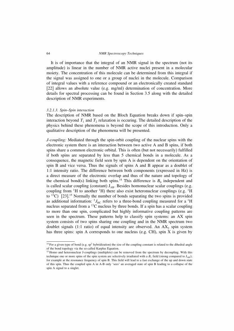
addition of 100–200mM phosphate buffer normalizes the pH in most cases toa range of 6.7–7.6, at least for several hours [59]. Nevertheless several smallmolecular endogenous metabolites present in biofluids show a pronounced pH-dependent chemical shift variation in 1H NMR spectroscopy even after buffering[62]. This is, for example, the case for citrate and histidine. The dependency of thecitrate resonances on pH is depicted in Figure 3.10. The remaining chemical shiftvariation (see also Section 3.2.2.1) between different samples has a direct impacton data reduction procedures and complicates further data evaluation steps. It maythus influence the data interpretation. Therefore, the binning of each spectrum intosegments with sufficiently large spectral width was introduced [63] to scope withthe shift variation (see also Section 3.6.2).
3.4.2.3. Salt concentration, EDTAAdjustment of pH of biological fluids alone does not fully remove the chemicalshift variation of organic acids like citrate [62], lactate, taurine or others. Furthereffects related to osmolality of the samples, ionic strength or metal ion composition
82 NMR Spectroscopy Techniques
pH 8
pH 7
pH 6
pH 5
pH 4
ppm 2.8 2.7 2.6
Figure 3.10. Variation of 1H NMR citrate chemical shifts at different pHs ranging from pH 4–8.
significantly contribute to the pH-independent chemical shift variation (see alsoSection 3.2.2). This is especially the case not only for urine and plasma but alsofor CSF or saliva [30].The inorganic metal ion composition of biological fluids, especially of urine, shows
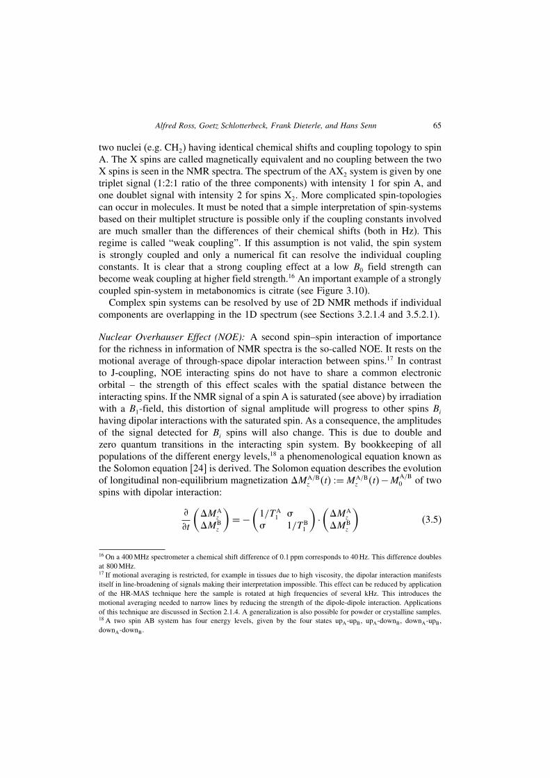
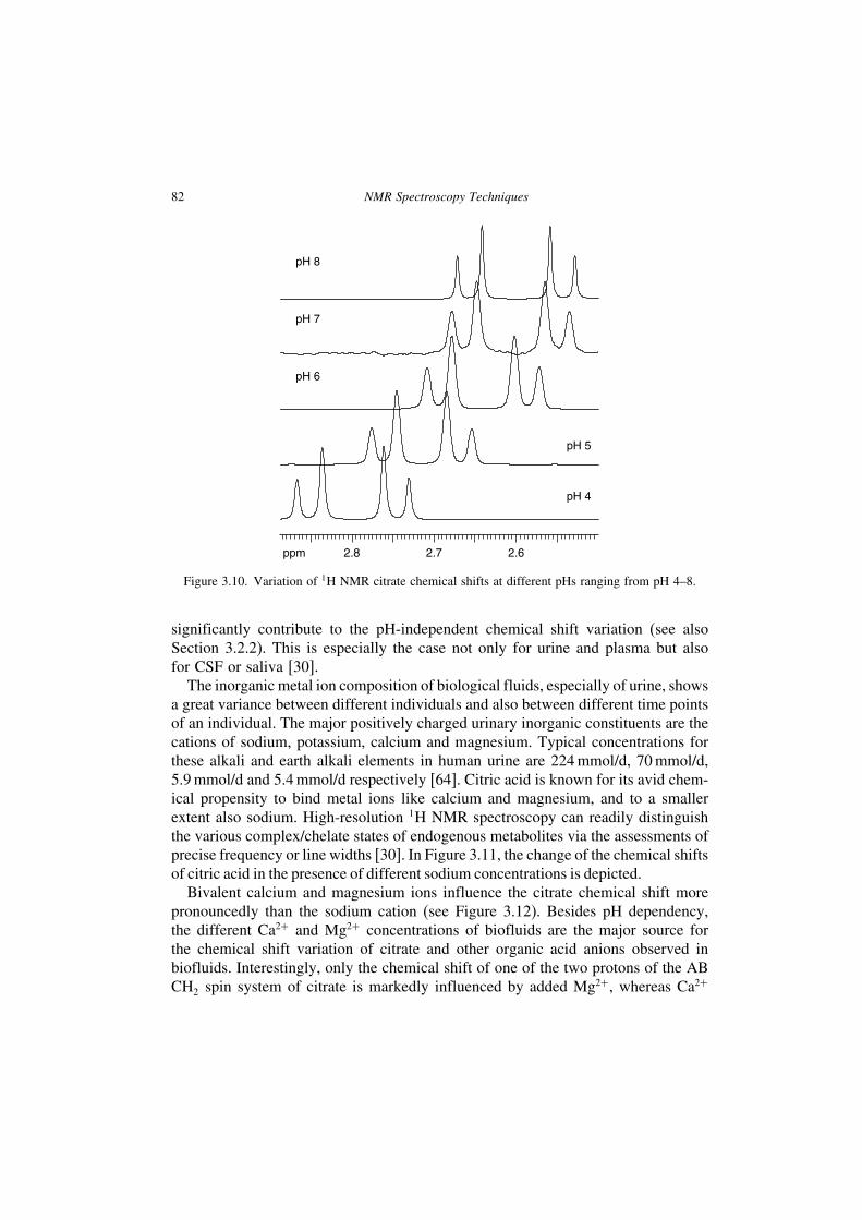
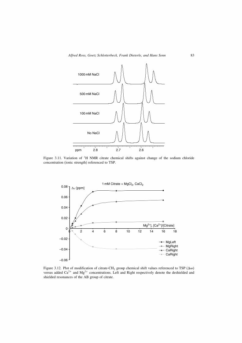
a great variance between different individuals and also between different time pointsof an individual. The major positively charged urinary inorganic constituents are thecations of sodium, potassium, calcium and magnesium. Typical concentrations forthese alkali and earth alkali elements in human urine are 224mmol/d, 70mmol/d,5.9mmol/d and 5.4mmol/d respectively [64]. Citric acid is known for its avid chem-ical propensity to bind metal ions like calcium and magnesium, and to a smallerextent also sodium. High-resolution 1H NMR spectroscopy can readily distinguishthe various complex/chelate states of endogenous metabolites via the assessments ofprecise frequency or line widths [30]. In Figure 3.11, the change of the chemical shiftsof citric acid in the presence of different sodium concentrations is depicted.Bivalent calcium and magnesium ions influence the citrate chemical shift more
pronouncedly than the sodium cation (see Figure 3.12). Besides pH dependency,the different Ca2+ and Mg2+ concentrations of biofluids are the major source forthe chemical shift variation of citrate and other organic acid anions observed inbiofluids. Interestingly, only the chemical shift of one of the two protons of the ABCH2 spin system of citrate is markedly influenced by added Mg2+, whereas Ca2+
Alfred Ross, Goetz Schlotterbeck, Frank Dieterle, and Hans Senn 83
1000 mM NaCl
No NaCl
100 mM NaCl
ppm 2.8 2.7 2.6
500 mM NaCl
Figure 3.11. Variation of 1H NMR citrate chemical shifts against change of the sodium chlorideconcentration (ionic strength) referenced to TSP.
0.081 mM Citrate + MgCl2, CaCl2
Mg2+], [Ca2+]/[Citrate]
∆ω [ppm]
0.06
0.04
0.02
–0.02
–0.04
–0.06
00 2 4 6 8 10 12 14 16 18
MgLeft
CaRightCaRight
MgRight
Figure 3.12. Plot of modification of citrate-CH2 group chemical shift values referenced to TSP (���versus added Ca2+ and Mg2+ concentrations. Left and Right respectively denote the deshielded andshielded resonances of the AB group of citrate.

84 NMR Spectroscopy Techniques
changed both resonances of the AB spin system. This may be attributed to differentstereochemistry of the Ca2+ and Mg2+ complexes due to differences in ionic radii(100 pm versus 72 pm [65] respectively).From an analytical and data evaluation point of view, a homogenous sample set
with respect to overall concentration, pH, metal ion composition and osmolalitywould be highly desirable, but for practical reasons the sample preparation can notaccount all these sources of variation in biofluids. For example, the adjustment of allsamples of a study to the same overall concentration can only be done with respectto the most dilute sample in the series. This would lead to drastically increasedexperimental acquisition times. As a compromise we propose the addition of per-deuterated EDTA to account for different earth alkali cation composition of biofluidsin addition to buffering. This is a simple modification of the sample preparationprocedure that fulfills most of the criteria mentioned in Section 3.4.2. The twomajor sources (pH and bivalent metal ion composition) of variation in chemicalshifts can be reduced. The span of chemical shifts for citrate can be dramaticallydecreased and peak overlap in different bins after data reduction can be avoided.This helps for statistical data analysis and simplifies the binning procedure (seeSection 3.6.2). Figure 3.13 shows the effect of addition of 10mM EDTA-d12 to80 samples of phosphate-buffered control rat urines. It can be clearly seen that notonly was the variation in citrate chemical shift minimized but also the potentialoverlap with a resonance of dimethylamine at �= 2.706 ppm was prevented. Thismodified procedure mainly affects the chemical shifts of chelating metabolites likecitric acid, taurine or lactic acid. The remaining signal of not fully deuterated EDTAis negligible and does not interfere with further data analysis steps.If creatinine is taken as a measure for urinary concentration24 and citrate chemi-
cal shifts are plotted against urinary concentration (creatinine) in a regime free ofinteraction between endogenous components, there should be no correlation visi-ble. However, the situation depicted in Figure 3.14 clearly shows a concentrationdependency of citrate chemical shifts in both cases with and without addition ofEDTA-d12. The variation of citrate resonance is reduced by a factor of about 2.4 instandard deviation after addition of EDTA-d12. The slope of the trend line indicatesremaining interaction modes of the non-chelated citrate with urinary componentswhich is concentration dependent, although less than in absence of EDTA.Besides the reduction in citrate chemical shift variation, the overall explained vari-
ance of a Principal Components Analysis (PCA) model is a measure for the effect ofEDTA-d12 addition. In Figure 3.15, the convergence of the explained variance of PCAmodels of 96 human urines with and without addition of EDTA-d12 is shown. The
24 This is valid to a good approximation for samples, where a drug induced change of creatinine signal can besafely excluded.

Alfred Ross, Goetz Schlotterbeck, Frank Dieterle, and Hans Senn 85
ppm 2.7 2.65 2.6 2.55
ppm 2.7 2.65 2.6 2.55
(a)
(b)
Figure 3.13. (a) Citrate chemical shift region of 80 rat urines buffered with 100mM phosphate buffer(pH 7.4). (b) Citrate chemical shift region of the same 80 rat urines buffered with 100mM phosphatebuffer and addition of 10mM EDTA-d12.
2.71
shift [ppm]
[Creatinine]
2.70
2.69
2.68
0 200 400 600 800 1000 1200
y = 0.0058x + 1340.1
y = 0.0095x + 1345.2
1400
Figure 3.14. Correlation of citrate chemical shift (centre of the low-field doublet) with (lower trace)and without EDTA-d12 (upper trace) against urine concentration represented by creatinine intensity.The standard deviation for citrate chemical shifts is reduced from ±31Hz to ±13Hz after additionof EDTA-d12, also the slope of the trend line is smaller.

86 NMR Spectroscopy Techniques
0
0.1
0.2
0.3
0.4
0.5
0.6
0.7
0.8
Comp[1] Comp[2] Comp[3] Comp[4] Comp[5]
EDTA no EDTA
Principal component
Convergence
R2X
(cum
)
Figure 3.15. Convergence of explained variance of PCA with integral normalized samples with andwithout EDTA-d12 addition.
explained variance increases faster after addition of EDTA-d12, therefore, the bene-ficial effect of decreased citrate variation is beneficial also for the complete data set.It can be seen that by removing one source of non-dose-dependent variation from thedata, the PCAmodels converge faster and statistical analysis should be facilitated.
3.5. NMR Experiments and their processing
Compared to other applications of NMR, the pulse sequences applied in metabo-nomics require a lower level of sophistication and the application of all sequencesis hampered by the following reason:All NMR experiments which rely on the detection of hydrogen nuclei (protons)
in biological samples face the problem that molecules have to be detected in anaqueous sample at M or lower concentrations against a background concentrationof 110M water protons. Thus a dynamic range of the receiver and digitizer systemof 108 would be needed. Modern state of the art receivers allow for 16-bit signaldigitization, ensuring a dynamic range below 106. Thus a suppression of the watersignal of at least 102 is required such that a signal of a compound at low concen-tration “fills at least a single bit”. A number of water suppression techniques havebeen reviewed in the NMR literature [66]. In the following, solvent suppressiontechniques and related pulse sequences that are applied in metabonomics analysiswill be described. The technique used for water suppression is of high importancefor the comparability between NMR data. Results obtained from multivariate anal-ysis of NMR spectra taken under different solvent suppression conditions can beerroneously interpreted as biological differences [62] if water suppression artifactsare not carefully excluded.

Alfred Ross, Goetz Schlotterbeck, Frank Dieterle, and Hans Senn 87
3.5.1. 1D NMR
Most applications of NMR for metabonomics research rely on 1D NMR experi-ments. This is dictated by long acquisition times of most multi-dimensional NMRexperiments making their application a time-consuming task for studies with largesample arrays. This situation is normally encountered for time- and dose-resolvedstudies with preclinical or clinical samples. Typical 1D NMR spectra of serum,urine and CSF are shown in Figure 3.16.
3.5.1.1. Water supressionPresaturation: The most widespread solvent suppression in use is the so-calledpresaturation technique [67]. This technique is applied in an NMR pulse methodknown as noesy-presat [68]. This pulse sequence is identical to the 1st time incrementof the 2D NOESY25 experiment (Figure 3.17). The water resonance is saturated by
10 9 8 7 6 5 4 3 2 1 0
1H [ppm]
Figure 3.16. 1D 1H NMR spectra from the top of serum, urine and CSF of rat. Very differentspectral signatures of the body fluids are clearly visible. The overall shape of the serum spectrumis dominated by a broad signal background having its origin in high-molecular weight compounds(proteins, lipoproteins). The eye-striking feature of urine is a huge urea signal at around 5.9 ppm,whereas the CSF spectrum is dominated by high glucose (3–4 ppm) and lactate (1.2 ppm) content.
25 Nuclear Overhauser Spectroscopy (NOESY): Here a 2D spectrum is acquired allowing for the determination ofdistances between protons within a molecule. The NOESY is widely applied in structure determination of proteinsby NMR1. The technique has found no application in metabonomics.

88 NMR Spectroscopy Techniques
φ 1
φ 1
φ 1 φ 1φ 2 φ 2
φ 1 – φ 4
φ 2 φ 3
φ rec
φ rec
φ rec
φ rec
1Hgradient
1Hgradient
1Hgradient
1Hgradient
yy yx
1/2G1/4G
1/8G1H [ppm]
(a)
(b)
(c)
(d)
G
6.0 5.5 4.8 4.7 4.6 4.5 4.4
Figure 3.17. Different methods of water suppression: From top to bottom the followingmethods together with typical results obtained for a urine sample are shown: (a)standard water presaturation of 3 s with 50Hz (phase cycling as follows: �1 = �rec =�x−x−xx y−y−y y��; (b) 1D noesy-presat during 3 s and 100 ms mixing time with50Hz (phase cycling: �1 = �x x−x−x�, �2 = �16x16�−x��, �3 = �4x4�−x�4y4�−y��,�rec = �2x4�−x�2x2y4�−y�2y2�−x�4x2�−x�2�−y�4y2�−y���; (c) WATERGATE with1ms selective pulses (phase cycling: �1 = �rec = �x y−x−y�, �2 = �1 + 180��; (d) WETwith 10ms selective shaped pulses – power levels of pulses compared to a 90� shapedpulse are +087−104+227−505dB counting from left to right (phase cycling: �1 =�y2�−y� y−x2x−x�, �2 = �−xx−xx−y y−y y�, �3 = �− y2y−y x2�−x� x�, �4 =�x−xx−x y−y y−y�, �rec = �2�x−x�2�y−y���. In the pulse schemes (a)–(d) shown to theleft, pulses on the top trace represent proton pulses (proton frequency). The heights of the pulse go inparallel with the applied B1 field strength. The bottom trace shows gradient pulses applied, wherebyall gradients are applied with sine shape. The black/grey shaded gradient pulses indicate applicationwith alternating sign of this pulse. The spectral region shown in the middle column shows the sizeof the urea signal. Urea protons experience chemical exchange with water. Therefore a substantialsuppression of this signal is seen for pulse methods which are “slow” on the exchange timescale (pre-saturation for 3 s in (a) and 2 s in (b) versus selective pulses of a few milliseconds for WATERGATEand WET). Therefore quantification of urea is not possible and the signal is typically excluded fromanalysis. Note: We have included here the phase cycling scheme that was employed. The addition ofscans is performed with different directions of applied pulses. This has to be done in concert withphase cycling of the receiver to obtain coherent addition of signals. Phase cycling is applied for thesetechniques to remove artifacts due to spectrometer imperfection and relaxation phenomena accruingduring the course of the pulse sequence.
frequency selective irradiation during the inter-scan delay and the mixing time ofthe sequence thus leading to a reduction of the equilibrium population differenceof the spin species resonating at the frequency of the weak (<50Hz) B1 fieldapplied. The big advantage of this method is given by a chemical shift selectivity

Alfred Ross, Goetz Schlotterbeck, Frank Dieterle, and Hans Senn 89
superior to any other technique. If a reliable quantification of signals resonatingclose to water (e.g. anomeric proton of glucose) is needed, this technique willbe the choice. The disadvantage of presaturation comes from the long duration(typically 2s). Therefore hydrogen atoms in chemical exchange with water (OH,NH, NH2� (see Section 3.2.2.1), protons having an NOE (see Section 3.2.1.3) witha proton under the water line, or which are exposed to a hydration shell will alsobe saturated. The degree of saturation is given by the rate of the chemical exchangeand the strength of the NOE respectively.26 Any interaction process slow on a 2stimescale can be neglected. The most prominent signal in urine exposed to saturationexchange is urea, which cannot be quantified if water presaturation is applied (seeFigure 3.17). This spectral region is excluded normally from metabonomics analysis.The mixing time, together with the intense phase cycling used in noesy-presat, has apositive effect on a flat baseline. This can be explained by a small degree of spatialselectivity27 encoded in the noesy-presat pulse sequence reducing the influence ofprotons entering or leaving the sensitive volume of the detection coil during thedetection of the FID. It must be noted that a mixing time will falsify the absoluteamplitudes of NMR signals detected due to differential T1, NOE and chemicalexchange effects.Experience in our laboratory shows that for cryogenic probeheads offering higher
sensitivity the quality of water suppression achievable by this technique is poorwhen measuring urine in 5mm sample tubes. In this case we have successfully useda sign-alternating gradient pulse applied between the end of the presaturation andthe first 90� pulse to significantly improve water suppression.In summary, the noesy-presat technique provides a simple, highly reproducible
and robust method for the acquisition of high-quality NMR spectra in aqueoussolutions. It has to be kept in mind, however, that absolute value quantification ispossible only with limited accuracy.
Gradient pulse based technique: This water suppression technique rests on theapplication of the so-called gradient pulses. A gradient pulse Gz (typically 1ms)creates an inhomogeneous magnetic field along the z-axis. Magnetization ofamplitude M0 present in the transverse plane prior to the pulse will be dephasedefficiently by Gz, as the frequency of the precession is z-dependent during Gz. Onlythe integral along the z-direction of the sample given by M0
∫ +z/2
−z/2 ei·�x·GzZ
′dZ′ ≈ 0 is
detected by the receiver. If the gradient is strong enough (>10G/cm), the signal is
26 This phenomenon is referred to as saturation transfer.27 Spatial selectivity of B1 pulses is obtained, as the distribution of the B1 field strength is not homogeneous over thesample. Therefore, long and/or many B1 pulses will lead to a reduction of signal amplitude. The region of highestB1 inhomogeneity is found at the upper and the lower rims of the sample. Therefore contributions of these regions(also prone to high B0 inhomogeneity and diffusion effects) are suppressed most efficiently by this technique.

90 NMR Spectroscopy Techniques
dephased by more than 99%.28 For the WET (water suppression enhanced throughT1 effects) [69] sequence which is used in metabonomics the transverse magnetiza-tion of the solvent signal is thus suppressed by the application of a series of weakfrequency selective B1 pulses, interleaved by Gz pulses. The flip-angles (durations)of the selective pulses and the strengths of the gradient pulses were optimized toachieve high-frequency selectivity, robustness and a flat baseline. The performanceof the sequence is further improved by the application of a composite 90� excitationpulse as the last pulse taking advantage of its higher spatial selectivity [27]. Effectsfrom chemical exchange and NOE are less serious for WET, as the overall durationof the sequence is more than one magnitude of order shorter compared to theduration of presaturation pulses described in above. The drawback is a reducedperformance in respect to frequency selectivity, having its origin in the higher B1
field strength typically used. All other parameters are essentially the same as innoesy-presat. The absence of the mixing time allows for an accurate quantificationhere. As a consequence, data taken with WET and noesy-presat cannot be analyzedstatistically in a combined data set but must be treated separately.
3.5.1.2. Editing techniquesRelaxation editing: Rigid molecules (e.g. proteins) with high molecular weightexperience a fast transverse relaxation (see Section 3.2.1). This is exploited inmetabonomics for the removal of signals of high-molecular-weight compounds.Thereby a 40–100 ms relaxation delay [70, 71] is included prior to data acquisition.J-coupling effects are most efficiently removed by use of the so-called CPMG(named after its inventors Carr Purcell Meiboom and Gill) [72] pulse sequencewith a refocusing delay set to 1ms. This technique is especially attractive for bloodserum or plasma samples having high content of proteins (see Figure 3.18). Forapplications on soft tissues the technique was successfully applied using a HR-MASprobe-head [73].
Diffusion editing: The principle of gradient pulses was introduced in Section 3.5.1.The application of a pair of z-direction gradient pulses of opposite sign will resultin a dephasing of transverse magnetization followed by a rephasing. No signal islost. This only holds true if the magnetization in a certain z-plane of the samplehas not moved to another z-plane between the application of the pair of gradientpulses. If a delay is inserted between the two gradients, rephasing is only partiallypossible due to Brownian motion and depending on the molecular weight of thesolute molecule. This phenomenon is used to remove signals from “small” molecules
28 Another important application of gradient pulses is the selection of coherence pathways. This technique allows,for example in HSQC type experiments, for the selection of signals of protons bound to 13C, and artefacts due toprotons bound to 12C are removed. For details, the reader is referred to citations in Section 3.5.2.2.

Alfred Ross, Goetz Schlotterbeck, Frank Dieterle, and Hans Senn 91
∆ ∆ δ
ε εn
3 3.2 3.02 1
ε ε
τm
1H [ppm]
Figure 3.18. Diffusion and T2 weighted filtration of a serum 1H NMR spectrum: The top row showsa 1D presaturation spectrum together with a boxed expansion. The middle row shows a spectrumand expansion with diffusion-weighted editing. A delay �m of 300ms serves to reduce signals fromlow-molecular-weight compounds (see triplet in expansion). The bottom row shows a CPMG-basedT2 weighted result. Here, n was set to 150 �150∗4� = 200ms� which reduces the broad lipoproteinhump in the background of the triplet substantially (see expansion).
which experience a high mobility [31]. To overcome fast signal decay due to T2
relaxation, the magnetization, dephased by the first gradient, is aligned along thez-axis and flipped back to the transverse plane prior to the 2nd gradient after50–300ms. This technique is referred to as PGSE (Pulsed Gradient Spin Echo)[74], whereby bipolar gradients [75] up to 100G/cm are used. An extension to2D by incrementation of the gradient strength is known by the acronym DOSY[76] (Diffusion Ordered Spectroscopy). This technique allows “the sorting” of thecompounds in a mixture according to their translation diffusion; applications formetabonomics research including tissues can be found in the literature [32, 77].
3.5.1.3. 13C spectroscopyThe chemical shift dispersion of 13C spins is higher by approximately a factor of20 when compared to protons. In addition, all signals in a 13C spectrum appearas singlets if 1H decoupling is applied15. Homonuclear 13C–13C scalar coupling isabsent due to the high dilution of 13C nuclei (only 1.11% of all carbon nuclei carry aspin). Thus the reduction in spectral complexity combined with substantially reducedspectral overlap would make the 13C nucleus an ideal candidate for metabolicprofiling. However, this is prohibited by the low intrinsic sensitivity of 13C detectiongiven by S13C = S1H · �3
13C · 0011 ≈ S1H · 34 · 10−4. Thus the acquisition of a 13C1D NMR spectrum that is identical in signal-to-noise to a 1H spectrum of thesame sample will need ∼108 times as long. Compromises in spectral amplitude areunpreventable and highest sensitivity equipment (13C cryogenic probehead togetherwith 900MHz) is absolutely compulsory. An additional gain in signal-to-noisecompared to 1H is of course seen as no spin multiplicities reduce the amplitude. Thesituation changes slightly if sensitivity enhancement by polarization transfer fromprotons (INEPT [78]) is used (see also 3.5.2.2).

92 NMR Spectroscopy Techniques
In the literature there is one example of a metabonomics analysis by use of 13Cspectra [79]. However, general use of 13C detection can only be recommended iffurther substantial improvements in sensitivity of the detection of NMR signals willbe achieved. What is of interest is the enrichment of 13C in biofluids or tissues byuse of 13C-labeled tracer molecules in biological studies. With this labeling approacha new window into metabolic analysis and diagnostics may be opened also in higherorganisms and metabolic pathway analysis including fluxes can be performed withacceptable sensitivity [80].
3.5.2. 2D NMR
It was mentioned before that a widespread use of 2D NMR in metabonomics islimited to small sample arrays by the long acquisition times needed. Neverthelessexamples of these techniques can be found in the literature and are applied inour laboratory. The 2D techniques unfold their full power if a de novo structuredetermination of a newly found metabolite in a biological sample is needed. Wewill not go into the process of structure determination here. The reader is referredto the expert literature [81].
3.5.2.1. Homonuclear 2D NMRJ resolved (J-Res): The most simple homonuclear 2D NMR experiment is the so-called J-resolved experiment [82]. Here J-coupling information is separated into a2nd dimension from the chemical shifts. The experiment was successfully appliedto many body fluids including urine [83], CSF�61�, seminal fluid [84] and bloodplasma [71]. An attractive feature of the 2D data matrix obtained is the calculationof a so-called chemical shift spectrum. It is obtained as a tilted projection of thefull 2D matrix. All signals (except those with strong coupling, e.g. citrate) appearas singlets positioned at the center of their respective multiplets in the standard 1Dcounterpart (see Figure 3.19). Thus the complexity of the spectrum is substantiallyreduced. The integral of signals in chemical shift spectra is strongly influenced byT2 relaxation. A straightforward way to use this data for absolute quantification ofconcentration is not possible, but comparison with a spectral database of metabolitesrecorded under identical experimental conditions might be promising for relativequantification. Typical experimental settings require the acquisition of 4–8 k com-plex data points along t2 for 32–128 t1 increments. An interscan delay of 2 s allowsfor T1 relaxation. Exponential or shifted sine-bell windowing is required along t2.Along t1 a sine or squared sine multiplication together with data summation can berecommended.
Correlation Spectroscopy (COSY) [85]: In this type of spectroscopy a cross-peak is obtained if two spins are connected by a homonuclear J-coupling (over
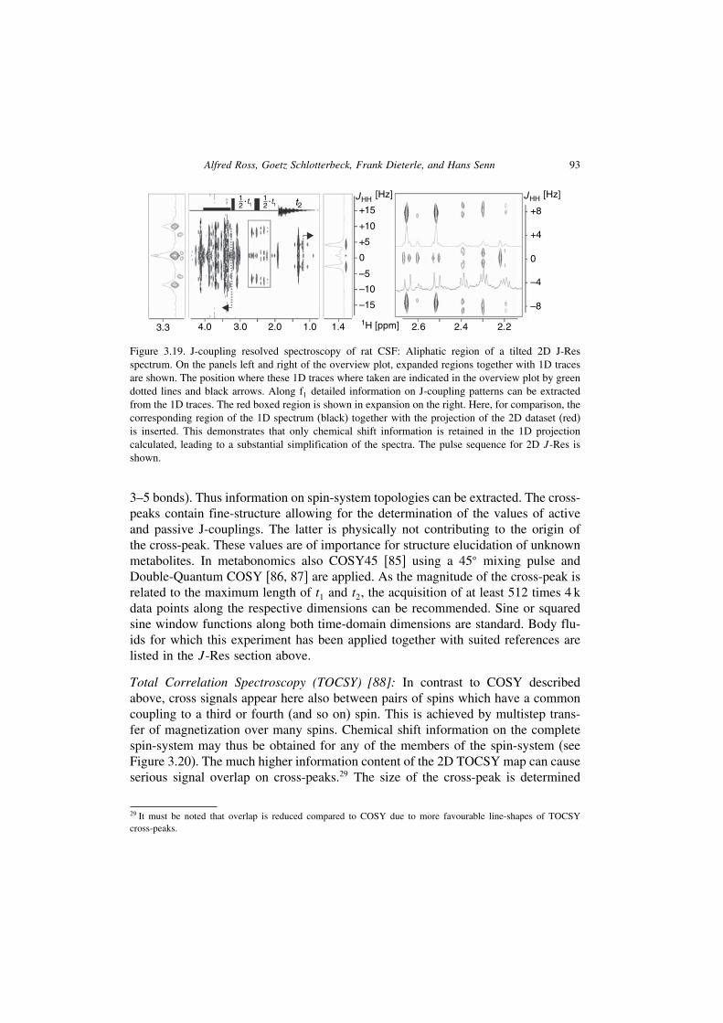
Alfred Ross, Goetz Schlotterbeck, Frank Dieterle, and Hans Senn 93
t2t112
t112
J HH[Hz]
1H [ppm]
–10
0
+5
+10
+15
–15
3.0 2.0 1.04.03.3 1.4 2.4 2.2
–8
–4
+4
+8
0
2.6
J HH [Hz]
–5
· ·
Figure 3.19. J-coupling resolved spectroscopy of rat CSF: Aliphatic region of a tilted 2D J-Resspectrum. On the panels left and right of the overview plot, expanded regions together with 1D tracesare shown. The position where these 1D traces where taken are indicated in the overview plot by greendotted lines and black arrows. Along f1 detailed information on J-coupling patterns can be extractedfrom the 1D traces. The red boxed region is shown in expansion on the right. Here, for comparison, thecorresponding region of the 1D spectrum (black) together with the projection of the 2D dataset (red)is inserted. This demonstrates that only chemical shift information is retained in the 1D projectioncalculated, leading to a substantial simplification of the spectra. The pulse sequence for 2D J -Res isshown.
3–5 bonds). Thus information on spin-system topologies can be extracted. The cross-peaks contain fine-structure allowing for the determination of the values of activeand passive J-couplings. The latter is physically not contributing to the origin ofthe cross-peak. These values are of importance for structure elucidation of unknownmetabolites. In metabonomics also COSY45 [85] using a 45� mixing pulse andDouble-Quantum COSY [86, 87] are applied. As the magnitude of the cross-peak isrelated to the maximum length of t1 and t2, the acquisition of at least 512 times 4 kdata points along the respective dimensions can be recommended. Sine or squaredsine window functions along both time-domain dimensions are standard. Body flu-ids for which this experiment has been applied together with suited references arelisted in the J -Res section above.
Total Correlation Spectroscopy (TOCSY) [88]: In contrast to COSY describedabove, cross signals appear here also between pairs of spins which have a commoncoupling to a third or fourth (and so on) spin. This is achieved by multistep trans-fer of magnetization over many spins. Chemical shift information on the completespin-system may thus be obtained for any of the members of the spin-system (seeFigure 3.20). The much higher information content of the 2D TOCSY map can causeserious signal overlap on cross-peaks.29 The size of the cross-peak is determined
29 It must be noted that overlap is reduced compared to COSY due to more favourable line-shapes of TOCSYcross-peaks.

94 NMR Spectroscopy Techniques
t1 t2MLEV
9 8 7 6 5 4 3 2 1 1H [ppm]
1
2
3
4
5
6
7
8
9
Figure 3.20. Total Correlation spectroscopy (TOCSY): The left panel shows an overview TOCSYspectrum taken from urine of one of the authors. Spin systems of metabolites can be identified as rowsof cross-signals correlating the chemical shifts of all spins involved in a spin system topology. Theinsert (left) shows a schematic drawing of the pulse sequence. The MLEV mixing sequence serves totransfer magnetisation along J-coupled networks. The right panel shows an expanded region correlatingprotons of aromatic moieties. As an example the spin system of hippurate is identified (right). It isimmediately clear which signals belong to the aromatic protons of this molecule. Another spin systemalso easily assigned in the same spectral region is that of indoxyl. Note: lecithin and pyridoxine, whichonly show singlet signals in the 1D, do not cause off-diagonal cross-signals in TOCSY. Accuratechemical shift measurements to distinguish both metabolites are mandatory. For comparison the 1Dspectra of all four compounds are shown at the bottom (right).
by the length of a so-called mixing sequence. In metabonomics [89] the MalcolmLevitt’s CPD sequence (MLEV) mixing sequence with duration of 80–300ms isapplied. Smaller t1/t2 data-matrices (e.g. 256∗2 k data points) are possible heremaking the application of squared cosine shaped window functions attractive. Alsoapplications to tissues employing HR-MAS are found in the literature [90, 73].A combination of TOCSY with diffusion editing (300ms diffusion delay) has alsobeen reported [32].
3.5.2.2. Heteronuclear correlation experimentsIn contrast to the direct 1D-based observation of 13C information, the indirectmeasurement via J-coupled 1H spins offers several advantages: (1) the sensitivity of

Alfred Ross, Goetz Schlotterbeck, Frank Dieterle, and Hans Senn 95
these class of experiments depends on the higher gyromagnetic ratio of the protons.As a consequence, 13C spins are observed with “only” 100 times reduced sensitivitycompared to 1H spectroscopy; (2) the chemical shift of the carbons is correlated withthe chemical shift of J-coupled protons. Several experiments found in metabonomicsmake use of these advantages.
Heteronuclear Single Quantum Coherence (HSQC) [71, 91, 92]: The chemical shiftof 13C is correlated via the large one-bond coupling constant 1JCH to the 1H chemicalshift of the directly bound proton (see Figure 3.21). Typical experimental settingsare a relaxation delay of 1s and a refocusing delay of 4.2ms. In total, 1024 datapoints with 200–300 scans for each of up to 512 t1 increments are acquired. Thespectral width is set to 140–180 ppm along the 13C dimension [93]. The standard forprocessing is a squared cosine window function applied along both dimensions. Itmust be noted, however, that the acquisition time for such an experiment will be inthe range of half a day making the application attractive only for selected samples.
20
13C [ppm]
1Ht2
t113C
30
40
50
60
70
80
4.5 4.0 3.5 3.0 2.5 2.0 1.5 1H [ppm]
decoupling
N
HN
HN
O
C H3
C H2
N
HN
HN
O
C H3
C H2
N
HN
HN
O
C H3
C H2
Figure 3.21. The schematic drawing of the HSQC sequence (HMBC not shown) is shown at the top.The 2D spectrum shows a superposition of a HSQC spectrum (blue) and a HMBC spectrum (red)of urine of one of the authors; only the aliphatic region is shown. Highlighted are the correlationsignals for the CH2 and CH3 groups of creatinine. The full circles show the direct 1JHC cross-peaksof the CH3 and CH2 group, respectively, in the HSQC spectrum (blue); the dotted circles highlightthe long range 3JHC cross-peak observed in the HMBC spectrum of the two groups. The direct andlong range correlations are also indicated in the structure (insert) with full blue and dotted red arrows,respectively. Many other very informative correlations are seen in the two 2D spectra. The acquisitionof these two data sets took one weekend of experimental measuring time.

96 NMR Spectroscopy Techniques
Heteronuclear Multiple Quantum Coherence (HMQC) [94]: The information con-tent obtained from this experiment is identical to that from HSQC. Applications inmetabonomics [79] reported 800 scans and 128 t1 increments. A short 500ms inter-scan relaxation is described in literature [95]. The same holds true for tissue-basedwork employing HR-MAS [90, 73]. A single example of the application of 1H-31PHMQC-TOCSY [96] can also be found. Here the 1H spin-system information,obtained via TOCSY transfer, is correlated with the chemical shift of phosphorous.This technique is not limited in sensitivity due to the high natural abundance of theNMR active phosphorous isotope.
Heteronuclear Multiple Bond Correlation (HMBC) [97]: With this experiment 13Cnuclei having a small multiple bond coupling nJCH are correlated via their chemicalshifts to 1H (see Figure 3.21). For each proton several cross signals related tocoupled 13C nuclei appear in the spectrum. The application in metabonomics [98]is hampered by the long experimental time. About 128–512 FIDs encompassing220 ppm 13C spectral width and up to 400 scans per increment are required. Alongt2, between 2 k and 32 k data points can be recorded. A squared sine-shaped windowfunction is recommended for processing. Typically a delay of 70ms was usedfor transfer of magnetization. The HR-MAS applications are described in literature[89, 90].
3.6. Data pre-processing
Data pre-processing can be seen as an intermediate step between recording of rawspectra and applying data analysis and modeling methods. Data pre-processingtransforms the data in a way that subsequent analyses and modeling are easier,more robust and more accurate. For NMR spectra from metabonomic studies, pre-processing methods are usually used to reduce variances and influences, whichare not of interest or which might interfere with data analysis. These variancescan be caused by measurements, by biology or by combined effects. Among theseeffects, NMR typical effects such as incorrect phases of the spectrum or varyingbaselines, animal study specific effects such as varying overall concentrations ofbiofluids and combined effects such as shifting peak locations in the spectrum playa role. Data pre-processing methods, which account for effects typical for NMRmeasurement and which are routinely applied to NMR spectra in many fields, arediscussed in Section 3.2.1.2. This section covers data pre-processing methods, whichare more specific for metabonomics. Data pre-processing for metabonomic studiesusually accounts for three effects discussed in the following sections, whereby notall pre-processing steps are mandatory.

Alfred Ross, Goetz Schlotterbeck, Frank Dieterle, and Hans Senn 97
3.6.1. Exclusion regions
Usually, the first step of data pre-processing is an exclusion of spectral regions,which contain non-reproducible information or which do not contain informationabout metabolites. Typically, the spectral width of recording NMR spectra is widerthan chemical shifts populated by endogenous metabolites. On the one hand, aminimum spectral width is predefined by a symmetrical range around the waterresonance when using water suppression techniques. On the other hand, a broadspectral width simplifies NMR pre-processing methods such as phasing and baselinecorrections. For the data analysis, spectral regions not populated by endogenousmetabolites are not useful. As these regions are sensitive to spectral artifacts suchas inadequate phasing, exclusion is beneficial. Therefore, the spectrum outside thewindow of 0.2–10 ppm is usually excluded. Other parts of the spectrum, which areusually excluded, are resonances of the solvent water. Although special suppressiontechniques for water resonances are used, the remaining signal of water, whichvaries due to different pre-saturation conditions, dominates the spectrum between4.6 ppm and 5.0 ppm rendering the analyses of signals of metabolites lying belowthe water resonances impossible. For spectra of urine, the signal of urea, which isvery close to water, is the most dominating peak besides that of water, as urea isthe most concentrated metabolite in urine. Yet, the urea peak is not quantitative, asthe protons exchange with water and consequently the peak intensity varies with thequality of water suppression (see Figure 3.17). As this peak has a high intensity anda broad range between 5.4 and 6.0 ppm, and as this peak varies, it highly influencesmethods of multivariate data analysis unless the peak is excluded.In many publications on the analysis of urine samples, the exclusion regions of
water and of urea are combined and the complete spectral region between 4.50 and5.98 ppm is excluded. Although this combination of exclusion areas also excludesspectral regions with signals of metabolites of interest (for example the resonanceof the �-anomeric proton of glucose at 5.24 ppm), it is the de facto standard inthe literature. Consequently, only the spectral range between 0.2 and 4.5 ppm andbetween 5.98 and 10 ppm is analyzed in the case of urine samples. For plasmasamples and extracts of tissue the spectral ranges from 0.2 to 4.6 ppm and from5.0 to 10 ppm are used, whereby additional exclusion regions might be necessarydepending on resonances of solvents for tissue extracts.
3.6.2. Peak shifts and binning
One of the major challenges for automated data analyses and peak assignments forspectra of biofluids from metabonomic studies is the effect of shifting peaks (seeSection 3.4.2). As the matrix of biofluids and, in particular, urine is highly varying,the local environment of protons also varies. Thereby many parameters play a role

98 NMR Spectroscopy Techniques
such as changes of the pH, changes of the salt concentration, overall dilution of thesample, relative concentrations of specific ions, relative concentration of specificmetabolites and many more. All these parameters can influence the shifts of peaks,whereby not all peaks are affected and different peaks are affected to a differentextent even when belonging to the same metabolite. In the left panel of Figure 3.22an example with 1H NMR spectra of 30 samples from a human metabonomic studyis shown. The clipping between 3.35 ppm and 3.49 ppm shows one singlet belongingto para-hydroxyphenylacetate and one triplet belonging to taurine. The position ofthe singlet is very stable at 3.455 ppm whereas the position of the taurine tripletvaries between 3.407 and 3.435 ppm. As the pH of the samples was constant due tobuffer added, the shifts of the taurine triplet are caused by different concentrationsof salts, of metal ions, of metabolites, or by varying dilutions of the samples.In a recent publication [99], it has been shown that peak shifts can be beneficial
for classifying groups of samples, if the locations of peaks are systematically dif-ferent between the various groups of samples. Yet, it is not possible to trace thesedifferences back to a single parameter such as systematic differences of pH, as manyparameters interact with peak shifts. In addition, the interpretation of classificationsand separations based on shifts of peaks is difficult, as the peak shifts are usuallyoverlaid by changes of the intensity of peaks due to changes of concentrations ofmetabolites. Consequently, the loadings of decomposition methods (PCA, partialleast squares (PLS), O-PLS) show distorted shapes of peaks, which need thoroughmanual interpretations. Therefore, a reduction of peak shifts either in silico or byspecial sample preparation methods (see Section 3.4.2.3) is most beneficial for themajority of applications. The mathematical approaches of reducing the influenceof peak shifts can be classified into two categories. The first widespread categoryreduces the resolution of spectra (by the so-called binning or bucketing procedures),whereas methods belonging to the second category try to align peaks.
Equidistant binning: The most popular methods of reducing the influence of shiftingpeaks are the so-called binning or bucketing methods, which reduce the resolution ofspectra.30 Thereby the spectra are integrated within small spectral regions, which arecalled “bins” or “buckets”. Subsequent data analysis procedures, which are appliedto the binned spectra, are not influenced by peak shifts, as long as these shiftsremain within the borders of the corresponding bins. The vast majority of 1H-NMRmetabonomics literature uses an equidistant binning of 0.04 ppm. This means thatthe spectrum is split into evenly spaced integral regions with a spectral width of0.04 ppm. In addition, it is common practice to sum up bins covering the citratedoublets (two bins per doublet) into super-bins, as the shifts of the two citrate
30 This reduction of resolution is not identical to that obtained by a lower B0 field strength. A multiplet with a totalwidth of 24Hz covers 0.04 ppm at 600 MHz. The ppm-width doubles at 300MHz.

Alfred Ross, Goetz Schlotterbeck, Frank Dieterle, and Hans Senn 99
doublets span more than one bin width each. With respect to exclusion areas thespectra are typically reduced to 206 bins visualized in Figure 3.23.The major drawback of equidistant binning is the non-flexibility of the boundaries.
If a peak crosses the border between two bins, this peak shift can significantlyinfluence the data analysis. For example, when analyzing binned spectra by PCAor PLS, peak shifts result in loadings with opposite signs. If the spectra shown inFigure 3.22 are binned by the wide-spread equidistant binning method with a binwidth of 0.04 ppm, the signal of the triplet of taurine is distributed among two bins(see Figure 3.22, left). The intensity assigned to each of the two bins highly dependson the exact location of the triplet. Thus, significant variance is added to the two bins,which is not related to the concentrations of taurine and para-hydroxyphenylacetate.Therefore the analysis of the concentrations of these metabolites on the basis ofthese bins is hampered.
Non-equidistant binning: To prevent peaks being cut by the boundaries of bins,binning methods have been proposed, which are based on non-equidistant spacingof bins. In the ideal case, the borders of the bins are adjusted in a way that bins coveronly complete peaks including all possible locations of the peaks. This means that thebin width depends on the width of the peak shape and on the shift width of the peak.An example is shown on the right side of Figure 3.22. None of the peaks is cut by the
Figure 3.22. Two different binning methods applied to a set of spectra. On the left side the boundariesof the widely used equidistant binning with a bin width of 0.04 ppm are shown. The right side showsthe boundaries of a non-equidistant binning method, which locates the boundaries of the bins intominima of mean spectra.

100 NMR Spectroscopy Techniques
1.02.03.04.05.06.07.08.09.0(ppm)
Figure 3.23. Spectrum before and after equidistant binning with a bin width of 0.04 ppm. In addition,two super bins for the citrate doublets were created and the spectral area between 4.5 and 5.98 ppmwas excluded. A vast majority of 1H NMR metabonomics literature uses this form of reduced spectrafor multivariate data analyses.
bin boundaries. The width of the bin covering the peak of para-hydroxyphenylacetateis narrow, as the peak does not shift. On the other side, the triplet of taurine is quitewide and shows extensive shifts. Therefore, the corresponding bin is very wide.The binning shown on the right side of Figure 3.22 is based on positioning the
borders of the bins on local minima of the mean spectrum of the set of controlspectra of the study. The considerable number of spectra results in a very smoothspectrum. Therefore, the local minima separate well between shifting peaks whileconserving each peak in a bin. For static peaks, the hyperfine structure is split intoseparate bins. Overall, 604 bins were generated for the spectral range of 0–10 ppmwith the water peak excluded.The unequal bin width also has some fundamental consequences for the subse-
quent data analysis. For the example discussed above the bin width varied between0.0014 and 0.46 ppm (broad peak of urea). If no further processing of the spectrumis performed, data points belonging to different bins influence the subsequent dataanalysis to a different extent. For example, a data point of a very small bin hasa higher influence than a data point of a very wide bin. If the subsequent dataanalysis is to represent the data points of the raw spectra as adequate as possible,it might be appropriate to scale the integral of the bins by the inverse of the binwidth. On the other side, each bin represents one single signal in the ideal case.Therefore the integral of a bin represents the “proton concentration” and with it theconcentration of the metabolite behind the signal. Thus, no further scaling is needed,if the data analysis is to be based on the concentrations of metabolites and changesof concentrations of metabolites.

Alfred Ross, Goetz Schlotterbeck, Frank Dieterle, and Hans Senn 101
A combination of equidistant binning and non-equidistant binning has been pro-posed and applied in metabonomics studies recently [100–102]. This method startswith the traditional bucket size of 0.04 ppm and allows the adjustment of the bordersby 50% resulting in a bin width between 0.02 and 0.06 ppm. The adjustment is basedon finding local minima of a sum of spectra or of a skyline projection of spectra.
Peak alignment: The alignment of peaks is an alternative to reducing the spectrumto account for peak shifts. A very promising approach has been proposed recently[37]. Thereby the spectra are segmented and the segments are shifted, stretchedand shrunken to maximize the correlation coefficient between the segments of aspectrum and a target spectrum. Overlapping connections after alignment are deletedand missing connections are interpolated. The optimal parameters are determinedeither by a genetic algorithm [37] or by a grid-search [103]. Although first resultsare very promising, further validation has to be performed as eliminations of peaks,changes of peak shapes and erroneous alignments cannot be excluded. Anotherapproach for the alignment of NMR spectra of complex mixtures with the samestrength and drawback has been proposed by Stoyanova [38]. In this approach peakshifts are identified by comparing a set of typical derivative shapes (e.g. derivativesof Lorentzian doublets with various coupling constants) with the loadings of thesecond principal component of the set of spectra. Identified regions with peak shiftsare aligned to a certain average frequency, whereby gaps are filled with zeros.
3.6.3. Normalization
A crucial step in data pre-processing of spectra from metabonomic studies is theso-called normalization. The normalization step tries to account for variations of theoverall concentrations of samples. Especially for urine, these variations of the overallconcentrations of samples are very distinctive. Urine of animals and humans cantypically be diluted by a factor of 4–5, whereby the dilution due to food deprivationor due to drug effects can exceed a factor of 10. In addition, sample preparation steps,such as addition of buffer, can further contribute to dilution of urine. In contrast tochanges of the overall concentration of urine, metabonomic responses and fluxesmainly influence only a few analytes in urine. Thereby concentrations of thesefew metabolites change specifically. These changes are visible as relative changesof concentrations of the few metabolites related to the concentrations of all othermetabolites, which represent the overall concentration of urine. Usually these relativespecific changes are of interest in metabonomic studies. Therefore, a normalizationstep, which compensates for differences of the overall concentration, is crucial, asvariations of overall concentrations obscure specific changes of metabolites. Besidescompensating for changes of the overall concentration of samples, normalization canalso be necessary due to technical reasons. If spectra are recorded using different

102 NMR Spectroscopy Techniques
number of scans or if spectra are recorded with different devices, the absolute valuesof the spectra are different rendering a joint analysis of the spectra without priornormalization impossible.All normalization procedures scale complete spectra in a way that these spec-
tra represent the same overall concentration. The scaling factor of each spectrumcorresponds to the dilution factor of the corresponding sample. In general, mostnormalization methods (also in other scientific fields) are special formulations ofthe general equation:
I�i�= Iold�i�
∑k
⎡⎣ juk∫
jlk
�I�x��ndx
⎤⎦
1n
(3.6)
Hereby Iold�i� and I�i� are the intensities of the variable i (spectral feature, wave-length, bin, chemical shift) before and after normalization, k is an index of thespectral regions used for normalization, jlk and juk are the lower and upper bordersof the spectral region k, for which the power n of the intensities I�x� are integrated.For the integral normalization, the power n is set to 1. Special variants of integral
normalization, such as creatinine normalization in metabonomics, use only parts ofthe spectral range. Thereby jlk and juk mark the borders of the k parts (e.g. left andright borders of the 2 creatinine peaks). The vector length normalization, which hasnot been used in the field of metabonomics up to now, uses a power n of 2. In thenext sections, the normalization procedures used in the field of metabonomics arediscussed in more detail.
Integral normalization: This method is the de facto standard of normalizing NMRspectra of biofluids. Integral normalization assumes that the integrals of spectra aremainly a function of the overall concentrations of samples. A linear concentrationseries of urine should result in a linear series of integrals of the corresponding spectra.Influences of changes of individual concentrations of single analytes are assumedto be small compared to changes due to varying overall concentrations of urine. Inaddition, specific down-regulations of metabolites should balance up-regulations ofmetabolites to a certain extent. The integral normalization procedure divides eachsignal or bin of a spectrum by the integral of the spectrum or part of it. Virtuallyall publications dealing with 1H-NMR metabonomics of urine samples exclude thespectral range of urea and water resonances from the integration and multiply eachvariable additionally by a factor of 100 ending up in a total integral of 100 for eachspectrum [37, 104–108].In Figure 3.24, two NMR spectra of rats from the same study are shown before
normalization and after normalization. The spectrum shown in black is diluted

Alfred Ross, Goetz Schlotterbeck, Frank Dieterle, and Hans Senn 103
1H [ppm]9 8 7 6 5 4 3 2 1 9 8 7 6 5 4 3 2 1
Figure 3.24. Two NMR urine spectra before normalization (left side) and after normalization (rightside). The black spectrum is diluted by a factor of 3 compared to the grey spectrum. After normalizationit is obvious that only very few differences of relative concentrations of metabolites between bothspectra exist.
by a factor of 3 compared to the grey spectrum. Therefore the spectra look verydifferent before normalization. The right side of the figure shows the two spectraafter normalization. Only very few differences are visible. These differences arebased on differences of relative concentrations of metabolites (specific differencesof the metabolic profiles) and are typically of interest. Before normalization thesedifferences were covered by the dilution effect.Although integral normalization is the de facto standard for NMR measurements
for metabolic profiling, the robustness, which is crucial for analysing highly varyingbiofluids, is the main weakness of the method. As soon as the integral of a spectrumis dominated not only by the overall concentration but also by specific changes ofmetabolites, the integral normalization does not scale the corresponding spectrumcorrectly. In Figure 3.25, an example of a sample is shown, which contains extreme
1H [ppm]9 8 7 6 5 4 3 2 1 1H9 8 7 6 5 4 3 2 1
Figure 3.25. Two NMR urine spectra after integral normalization (left side) an optimal normalization(right side, quotient normalization). The black spectrum contains massive amounts of glucose due toa glucosuria of the animal. As the peaks of glucose account for 75% of the integral of the spectrum,the integral normalization method has incorrectly downscaled the spectrum by a factor of 0.25. Anoptimal normalization shown on the right side reveals that besides the extreme amounts of glucosehardly any differences between the two samples exist.

104 NMR Spectroscopy Techniques
amounts of glucose due to glucosuria of the corresponding animal. As the peaks ofglucose account for 75% of the integral of the spectrum, the integral normalizationhas downscaled the complete spectrum by a factor of 0.25 compared to an optimalnormalization. Besides the presence of extreme amounts of endogenous metabolites,drug metabolites, for which the signals were not excluded or replaced, can alsodramatically mislead the integral normalization.
Creatinine Normalisation: This method is a special version of the integral nor-malization originating from clinical chemistry. For the investigation of urine ofhumans and animals in clinical chemistry, it is a common procedure to normalizeconcentrations of analytes by the concentration of creatinine [111, 112–114]. Theassumption is a constant excretion of creatinine into urine (often referred to ascreatinine clearance). Thus, creatinine is an indicator of the concentration of urine.As the concentration of creatinine can be determined by its peaks in the spectra(peaks at 3.05 and 4.05 ppm), it has been proposed in early publications to normalizespectra by the concentration of creatinine [113].Yet, the practical application of the creatinine normalization is faced by technical
and biological difficulties. From the technical point of view, metabolites with over-lapping peaks can interfere with the determination of the creatinine concentration(e.g. creatine at 3.04 ppm). In addition, the chemical shift of creatinine at 4.05 ppmdepends on the pH of samples rendering a sophisticated peak picking algorithmnecessary. Biological challenges for creatinine normalization are changes of the con-centrations of creatinine due to metabonomic responses, which has been shown inseveral studies [114]. In that case, the normalization by creatinine is worthless. As atthe step of normalization of spectra a possible increase of the creatinine level due tometabonomic responses is usually not yet known, a creatinine-based normalizationis not of general use in metabonomics.
Quotient normalization: Recently, a new approach of normalization has been pro-posed [115], which is based on the assumption that changes in concentrations ofsingle analytes only influence parts of the spectra, whereas changes of overall con-centrations of samples influence the complete spectrum. Instead of the assumptionof a constant total integral of the integral normalization, a most probable quotientbetween a spectrum and a reference spectrum is calculated as normalization fac-tor. This most probable quotient for a specific spectrum can be derived from thedistribution of each bin (variable, spectral value, data point) of a spectrum dividedby the corresponding bin of a reference spectrum. In Figure 3.26, two histogramsof the distributions for the quotients of two spectra each are shown. The histogramon the left side represents the quotients of the 205 bins of the black and grey spec-trum shown in the left part of Figure 3.24. It is clear that the distribution of thequotients is rather sharp. The most probable quotient is located around 0.33, whichcorresponds to a threefold dilution of the black spectrum. The histogram on the right

Alfred Ross, Goetz Schlotterbeck, Frank Dieterle, and Hans Senn 105
0102030405060708090
0
0.1
0.2
0.3
0.4
0.5
0.6
0.7
0.8
0.9 1
Quotient
0
10
20
30
40
50
60
0
0.1
0.2
0.3
0.4
0.5
0.6
0.7
0.8
0.9 1
Quotient
Fre
quen
cy
Fre
quen
cy
Figure 3.26. Histograms for the distributions of the quotient of two spectra each. The left histogramrepresents the quotients of the two spectra each shown in the left part of Figure 3.24. The dilutionfactor of 3 of the black spectrum is represented as most probable quotient around 0.33. The righthistogram represents the quotients of the two spectra shown in the left part of Figure 3.25. The mostprobable quotient is around 0.25. The dominance of the glucose peaks is only visible as a rather smallbar for quotients higher than 1 (last bar on the right side).
side of Figure 3.26 represents the quotients of the two spectra shown in the left partof Figure 3.25. The distribution shows that the most probable quotient is around0.25. This corresponds to the incorrect downscaling of the black spectrum by theintegral normalization, as the glucose peak contributes 75% to the total integral.The dominance of the glucose peak hardly influences the distribution and the mostprobable quotient. It is only visible as rather small bar on the right side, whichrepresents quotients higher than 1.The quotient normalization is based on the robustness of the distribution of
quotients in contrast to integrals. The most probable quotient, which is needed forthe normalization, can be estimated in several ways. Using the median as estimationof the most probable quotient has been proven to be a very robust and very exactmethod. For the calculation of the quotients, a reference spectrum is needed incontrast to integral normalization. The reference spectrum can be a single spectrumof the study, a “golden” reference spectrum from a database, or a calculated medianor mean spectrum on the basis of all spectra of the study or on the basis of a subsetof the study. It has been shown that the choice of reference spectrum is uncritical,and a median spectrum of control animals seems to be the most robust referencespectrum for studies with only few animals. It is also recommended to perform anintegral normalization prior to quotient normalization to scale different studies tothe same absolute magnitude. The algorithm of the quotient normalization can besummarized as follows:
1. Perform an integral normalization (typically a constant integral of 100 is used)2. Choose/calculate a reference spectrum (best approach: calculate median spectrum
of control samples).

106 NMR Spectroscopy Techniques
3. Calculate the quotients of all variables of interest of the test spectrum with thoseof the reference spectrum.
4. Calculate the median of these quotients.5. Divide all variables of the test spectrum by this median.
The quotient normalization can be applied to raw spectra or to binned spectra,but variables not containing signals should be excluded from calculating the mostprobable quotient if possible.The robustness of the quotient normalization can be seen in Figure 3.25. The
integral normalization is heavily hampered by massive amounts of glucose in thesample represented by the black spectrum. Therefore the spectrum shown in black isincorrectly downscaled (left part of the figure). On the right side of Figure 3.25, theresults of the quotient normalization are shown. It is clear that the quotient normal-ization is not influenced by the glucose peak, but performs an ideal normalization:The quotient normalization reveals the high similarity of both spectra representingnearly identical relative concentration levels of most metabolites except glucose.This similarity remains hidden when using the integral normalization.The quotient normalization performs better than the integral normalization not
only in the case of very intense signals due to strong metabolic responses or due todrug metabolites, but also in the case of “normal” spectra of control animals showingonly small normal metabolic variations. For example, 4023 spectra from controlanimals and pre-dosed animals were normalized by the total integral normalizationprocedure and by the quotient normalization procedure. As all animals had not beendosed, the creatinine levels of the samples were not influenced by metabonomicchanges and consequently represent a good measure for the overall concentration ofsamples. The variations of the creatinine levels, which can be seen as performanceindicator for the normalization, are 7.6% for the integral normalization and 6.7% forthe quotient normalization. This means that even when looking at control animals,small specific variations due to metabonomic fluxes negatively impact the integralnormalization.A drawback of the quotient normalization compared to integral normalization
is the absence of a fixed independent absolute reference value (e.g. a total inte-gral of 100). This renders a re-normalization of a combined data set necessary,if two data sets which were normalized separately are merged or compared. Thisre-normalization can be prevented if a common reference spectrum is used for theseparate normalizations of various data sets.
3.7. Outlook
The intrinsic properties of complex biological samples will continue to be a bigchallenge for NMR in metabolic analysis:

Alfred Ross, Goetz Schlotterbeck, Frank Dieterle, and Hans Senn 107
• Metabonomics fundamentally rests on large sample arrays. Perfect control of allspectral parameters (including chemical shifts) in mixtures cannot be achieved. Asa consequence, assigning corresponding variables across different samples of oneand the same study to the same molecular structure is of paramount importance.NMR will have to deal with “imperfect” samples although improvements insample preparation are certainly possible.
• Currently there is a severe “assignment gap” – many NMR peaks in body fluidsare not assigned to metabolites. Recourse to pattern-only analysis without know-ing their most prominent molecular features is unsatisfactory for mechanisticalbiochemical interpretation.
• In principle, using NMR spectroscopy submicrogram quantities can be quantified.However, this is possible in practice only if signals of high amplitude do notoverlap with small signals. This prerequisite is not fulfilled for biological samples,where concentration ranges of metabolites can span several orders of magnitude.Large changes of compounds that are low in concentration can only be detectedif signal overlap is avoided. Here liquid chromatography (LC)-based separationtechniques might come into play combined with NMR. It might well be that thefundamental “dogma” of metabonomics “no sample preparation needed” will soonhave to be revisited.
Thus from the NMR spectroscopic point of view, complete profiling of biologicalmixtures will remain difficult for very fundamental technology reasons.The ongoing development of NMR is addressing some of these problems:
• The trend to higher field-strength will improve the analysis of crowded spectra.More metabolites will become visible without overlap of lines. The 1GHz magnetis within reach. Nevertheless the dynamic range problem in signal intensity com-bined with signal overlap will always cause difficulties in the detailed analysis ofmetabolites that are low in concentration.
• The introduction of cryogenic probeheads has improved the sensitivity of detectionwithin the last 10 years by a factor of 4–5. Now it is a fact that for aqueousbiological samples the “sample noise” is one limiting factor of NMR sensitivity.It seems unlikely that NMR devices will be available in the mid-term futurewhich will allow the detection of compounds which are orders of magnitudelower in concentration than those analyzed today. We estimate that less than 100metabolites in urine provide more than 95% of the total signal amplitude, and thiswill be true at any given sensitivity.
• The low concentration and the high range to be detected prevent the applicationof multi-dimensional NMR techniques, which could resolve the overlap problemfor large sample arrays. Due to the extensive measuring times needed for dilutedsamples, these methods can be employed only for very focused questions like thede novo determination or verification of the structure of an unknown endogenous

108 NMR Spectroscopy Techniques
or xenobiotic metabolite. There is no obvious gap in the availability of NMR pulsesequences. Nevertheless improvement in details (see Section 3.5.1.1) is needed toadjust the pulse sequence to the given sample and problem.
Having said that, we foresee the two following main developments in NMR methodsthat will open new avenues in metabonomic analysis:
• Currently different vendors of NMR spectrometer and industrial research groupsare building up spectral databases [116] of metabolites known to be present inbiological samples at concentrations visible in NMR. The aim of these effortsis to develop an analysis tool for a priori assignment of spectra of biofluids toindividual metabolites. The analysis rests today almost exclusively on multivariateanalyses of spectral features and patterns, in order to identify and extract signifi-cant peaks which are a posteriori assigned. The a priori assignment would openup a window to concentration values of hundreds of known metabolites [117].Different software companies [116, 118, 119] are working on algorithms to allowextraction of this information by interactive analysis of 1D NMR spectra.
• A second development expected to have impact in the field is the concertedanalysis of data acquired with different analytical methods on the same sample(NMR, GC-MS, LC-MS) [120]. The richness of information to be obtained bythis approach cannot be overestimated.
We expect that both developments will have a substantial impact on the proliferationof metabolite profiling methods in wide fields of discovery and applied medicalresearch.
References
[1] K. Wüthrich, NMR of Proteins and Nucleic Acids, Wiley and Sons, New York, 1986.[2] D.G. Gadian, NMR and its application to living systems Oxford University Press, Oxford, 1995.[3] F.F. Brown, I.D. Camplell, P.W. Kuchel, D.C. Rabenstein, FEBS Lett. 82 (1977) 12.[4] J.R. Bales, D.P. Higham, I. Howe, J.K. Nicholson, P.J. Sadler, Clin. Chem. 30 (1984) 426.[5] J.K. Nicholson, I.D. Wilson, Prog. NMR Spectrosc. 21 (1989) 449.[6] Bell, J.D. MRS in biology and medicine, Eds J.D. de Certaines, W.M.J. Bovee, F. Bodo,
Pergamon Press, Oxford.[7] J.K. Nicholson, J. Conelly, J.C. Lindon, E. Holmes Nature Reviews, Drug Disc. 1 (2002) 153.[8] J.C. Lindon, J.N. Nicholson, E. Holmes, H. Antii, E. Bollard, H. Keun, O. Beckonert, T. Ebbels,
M. Reily, D. Robertson, G. Stevens, P. Luke, A. Breau, G. Cantor, R. Bible, U. Niederhauser,G. Schlotterbeck, H. Senn, U. Sidelmann, A. Laursen, A. Tymiak, B. Car, L. Lehman, J.-M.Colet, C. Thomas, Tox. Appl. Pharm. 187 (2003) 137.
[9] A.R. Fernie, R.N. Tethewey, A.J. Krotzky, L.W. Willmitzer, Nature Reviews, Molec. Cell Biol.5 (2002) 1.

Alfred Ross, Goetz Schlotterbeck, Frank Dieterle, and Hans Senn 109
[10] R. Ernst, G. Bodenhausen, A. Wokaun, Principles of Nuclear Magnetic Resonance in One andTwo Dimensions, Oxford University Press, Oxford, 1990.
[11] M. Goldman, Quantum Description of High-Resolution NMR in Liquids, Oxford UniversityPress, Oxford, 1991.
[12] J.L. Sudmeier, S.E. Anderson, J.S. Frye, Conc. Magn. Reson. 2 (1990) 197.[13] Q.N. Van, G.N. Chmurny, T.D. Veenstra, Biochem. Biophys. Res. Comm. 301 (2003) 952.[14] P.T. Callaghan, Principles of Nuclear Magnetic Resonance Microscopy, Oxford University
Press, Oxford, 1991.[15] P.F. Flynn, D.L. Mattiello, H.D.W. Hill, A.J. Wand, J. Am. Chem. Soc. 122 (2000) 4824.[16] D. Moskau, Concepts Magn. Reson. 15 (2002) 164.[17] G. Schlotterbeck, A. Ross, R. Hochstrasser, H. Senn, T. Kühn, D. Markek, O. Schett, Anal.
Chem. 74 (2002) 4464.[18] D.L. Olson, T.L. Peck, A.G. Webb, R.L. Magin, J.V. Sweedler, Science 270, (1995) 1967.[19] T. Horiuchi, M. Takahashi, J. Kikuchi, S. Yokoyama, H. Maeda, J. Magn. Reson. 174 (2005)
34.[20] J.C. Hoch, A.S. Stern , NMR Data Processing, John Wiley & Sons Inc. New York, 1997.[21] D.D. Traficante, M. Rajabzadeh, Conc. Magn. Reson. 12 (2000) 83.[22] V. Silvestre, S. Goupry, M. Trierweiler, R. Robins, and S. Akoka, Anal. Chem. 73 (2001) 1862.[23] R. Freeman, E. Kupce, NMR in Biomed. 10 (1997) 272.[24] I. Solomon, Phys. Rev. 99 (1955) 559.[25] W.P. Aue, E. Bartholdi, R.R. Ernst, J. Chem. Phys. 64 (1976) 2229.[26] A. Ross, G. Schlotterbeck, W. Klaus, H. Senn, J. Biomol. NMR 16 (2000) 139.[27] O. Cloarec, M.-E. Dumas, A. Craig, R.H. Barton, J. Trygg, J. Hudson, C. Blancher, D. Gauguier,
J.C. Lindon, E. Holmes, J. Nicholson, Anal. Chem. 77 (2005) 1282.[28] H.M. McConnell, J. Chem. Phys 28 (1958) 430.[29] L.Y. Lian, G.C.K. Roberts, NMR of Macromolecules – A Practical Approach, IRL Press,
Oxford, 1993.[30] C.J.L. Silwood, M. Grootveld, E. Lynch, J. Biol. Inorg. Chem. 7 (2002) 46.[31] E.O. Stejskal, J.E.J. Tanner, Chem. Phys. 42 (1965) 288.[32] M. Liu, J.K. Nicholson, J.C. Lindon, Anal. Chem. 68 (1996) 3370.[33] J.D. Otvos, E.J. Jeyarajah, D.W. Bennett, Clin. Chem. 37 (1991) 377.[34] M. Pellechia, D.S. Sems, K. Wüthrich, Nature Rev. Drug Disc 1 (2002) 211.[35] P.J. Hajduk, T. Gerfin, J.M. Boehlen, M. Häberli, D. Marek, S.W. Fesik, J. Med. Chem. 42
(1999) 2315.[36] J.C. Lindon, E. Holmes, J.K. Nicholson, Prog. in NMR Spectrosc. 45 (2004) 109.[37] J. Forshed, I. Schuppe-Koistinen, S.P. Jacobssen, Anal. Chim. Acta 487 (2003) 189.[38] R. Stoyanova, A.W. Nicholls, J.K. Nicholson, J.C. Lindon, T.R. Brown, J. Magn. Reson. 170
(2004) 329.[39] G.C. Lee, D.L. Woodruff, Anal. Chim. Acta. 513 (2004) 413.[40] T.L. Peck, R.L. Magin, P.C. Lauterbur, J. Magn. Reson. 108 (1995) 114.[41] G.E. Martin, R.C. Crouch, A.P. Zens, Magn. Reson. Chem. 36 (1998) 551.[42] W.L. Fitch, G. Detrer, C.P. Holmes, J.N. Shoolery, P.A. Keifer, J. Org. Chem. 59 (1994) 7955.[43] D.L. Olson, J.A. Norcross, M. O’Neil-Johnson, P.F. Molitor, D.J. Detlefsen, A.G. Wilson,
T.L. Peck, Anal. Chem. 76 (2004) 2966.[44] H. Kocacs, D. Moskau, M. Spraul, Prog. NMR Spectrosc. 46 (2005) 131.[45] A. Geiger, M. Holz, J. Phys. E: Sci. Instrum. 13 (1980) 697.[46] C.G. Wade, R.D. Johnson, S.B. Philson, J. Strouse, F.J. McEnroe, Anal. Chem. 61 (1989)
107A.

110 NMR Spectroscopy Techniques
[47] M. Spraul, M. Hofmann, M. Ackermann, A.W. Nicholls, S.J.P. Damment, J. N. Halselden,J.P. Shockcor, J.N. Nicholson, J.C. Lindon, Anal. Commun. 34 (1997) 339.
[48] P.A. Keifer, Drug Disc. Today 2 (1997) 468.[49] A. Ross, H. Senn, Drug Disc. Today 6 (2001) 583.[50] A. Ross, H. Senn, Curr. Top. Med. Chem. 3 (2003) 55.[51] N.T. Holland, M.T. Smith, B. Eskenazi, M. Bastaki, Mutat. Res. 543 (2003) 217.[52] COMET Consortium internal presentation O. Beckonert, 2002.[53] S. Deprez, B.C. Sweatman, S.C. Connor, J.N. Haselden, C.J. Waterfield, J. Pharm. Biomed.
Anal. 30 (2002) 1297.[54] D.K. Hansen, M.I. Davies, S.M. Lunte, C.E. Lunte, J. Pharm. Sci. 88 (1999) 14.[55] K.E. Price, S.S. Vandaveer, C.E. Lunte, C.K. Larrive, J. Pharm. Biomed. Anal. 38 (2005) 904.[56] P. Khandelwal, C.E. Beyer, Q. Lin, L.E. Schechter, A.C. Bach, Anal. Chem. 76 (2004) 4123.[57] P. Khandelwal, C.E. Beyer, Q. Lin, P. McGonigle, L.E. Schechter, A.C. Bach, J. Neurosci.
Methods 133 (2004) 181.[58] O. Fiehn, Plant Molec. Biol. 48 (2002) 155.[59] J.C. Lindon, J.K. Nicholson, E. Holmes, J.R. Everett, Concepts Mag. Reson. 289 (2000) 12.[60] H.C. Keun, T.M.D. Ebbels, H. Antti, M.E. Bollard, O. Beckonert, G. Schlotterbeck, H. Senn,
U. Niederhauser, E. Holmes, J.C. Lindon, J.K. Nicholson, Chem. Res. Toxicol. 15 (2002) 1380.[61] B.C. Sweatman, R.D. Farrant, E. Holmes, F.Y. Ghauri, J.K. Nicholson, J.C. Lindon, J. Pharm.
Biomed. Anal. 11 (1993) 651.[62] B.C.M. Potts, A.J. Deese, G.J Stevens, M.D. Reily, D.G. Robertson, J. Theiss, J. Pharm.
Biomed. Anal. 26 (2001) 463.[63] R.D. Farrant, J.C. Lindon, E. Rahr, B.C. Sweatman, J. Pharm. Biomed. Anal. 10 (1992) 141.[64] Ciba-Geigy, Eds, Wissenschaftliche Tabellen Geigy, vol. 1, 8th edn, Ciba-Geigy, Basel, 1980.[65] N.N Greenwood, A. Earnshaw, Chemistry of the elements, Pergamon Press, Oxford, 1986.[66] W.S Prince, Ann. Rep. NMR Spectr. 38 (1999) 289.[67] D.I. Hoult , J. Magn. Reson 21 (1976) 337.[68] A. Kumar, R.R. Ernst, K. Wüthrich, Biochem. Biophys. Res. Commun. 95 (1980) 1.[69] R.J. Ogg, P.B. Kingsley, J.S. Taylor, J. Magn. Reson. 104B (1994) 1.[70] E.M. Lenz, J. Bright, I.D. Wilson, S.R. Morgan, A.F.P. Nash, J. Pharm. Biomed. Anal. 33
(2003) 1103.[71] J.K. Nicholson, P.J.D. Foxall, M. Spraul, R.D. Farrant, J.C. Lindon, Anal. Chem. 67 (1995) 793.[72] S. Meiboom, and D. Gill, Rev. Sci. Instrum. 29 (1958) 688.[73] M.E. Bollard, S. Garrod, E. Holmes, J.C. Lindon, E. Humpfer, M. Spraul, and J.K. Nicholson,
Magn. Reson. Med. 42 (2000) 201.[74] S.J. Gibbs, and C.S. Johnson Jr, J. Magn. Reson. 93 (1991) 395.[75] G. Wider, V. Dötsch, K. Wüthrich, J. Magn. Reson. 108A (1994) 255.[76] K.F. Morris, C.S. Johnson Jr, J. Am. Chem. Soc. 114 (1992) 3139.[77] J.L. Griffin, H.J. Williams, E. Sang, and J.K. Nicholson, Magn. Reson. Med. 46 (2001) 249.[78] G.A. Morris, R. Freeman, J. Am. Chem. Soc. 101 (1979) 770.[79] H.C. Keun, O. Beckonert, J.L. Griffin, C. Richter, D. Moskau, J.C. Lindon, J.K. Nicholson,
Anal. Chem. 74 (2002) 4588.[80] J.G. Jones, M.A. Solomon, A.D. Sherry, F.M.H. Jeffrey, C.R. Malloy, Am. J. Physiol. 275
(1998) E843.[81] H. Günther, NMR Spectroscopy, Wiley & Sons Inc. New York, 1992.[82] W.P. Aue, J. Karhan, R.R. Ernst, J. Chem. Phys. 64 (1976) 4226.[83] E. Holmes, P.J.D. Foxall, M. Spraul, R.D. Farrant, J.K. Nicholson, J.C. Lindon, J. Pharm.
Biomed. Anal. 15 (1997) 1647.

Alfred Ross, Goetz Schlotterbeck, Frank Dieterle, and Hans Senn 111
[84] M.J. Lynch, J. Masters, J.P Pryor, J.C. Lindon, M. Spraul, P.J.D. Foxall, J.K. Nicholson,J. Pharm. Biomed. Anal. 12 (1994) 19.
[85] A. Bax, and R. Freeman, J. Magn. Reson. 44 (1981) 542.[86] A. Derome, and M. Williamson, J. Magn. Reson. 88 (1990) 177.[87] B. Ancian, I. Bourgeois, J.-F. Dauphin, and A.A. Shaw, J. Magn. Reson. 125A (1997) 348.[88] A. Bax, and D.G. Davis, J. Magn. Reson. 65 (1985) 355.[89] A.W. Nicholls, E. Holmes, J.C. Lindon, J.P. Shockcor, R.D. Farrant, J.N. Haselden,
S.J.P. Damment, C.J. Waterfield, J.K. Nicholson, Chem. Res. Toxicol. 14 (2001) 975.[90] S. Garrod, E. Humpfer, M. Spraul, S.C. Connor, S. Polley, J. Connelly, J.C. Lindon,
J.K. Nicholson, E. Holmes, Magn. Reson. Med. 41 (1999) 1108.[91] A.G. Palmer III, J. Cavanagh, P.E. Wright, M. Rance, J. Magn. Reson. 93 (1991) 151.[92] L.E. Kay, P. Keifer, T. Saarinen, J. Am. Chem. Soc. 114 (1992) 10663.[93] S. Ringeissen, S.C. Connor, H.R. Brown, B.C. Sweatman, M.P. Hodson, S.P. Kenny,
R.I. Haworth, P. Mcgill, M.A. Price, M.C. Aylott, D.J. Nunez, J.N. Haselden, C.J. Waterfield,Biomarkers 8 (2003) 240.
[94] R.E. Hurd, B.K. John, J. Magn. Reson 91 (1991) 648.[95] A.W. Nicholls, J.K. Nicholson, J.K. Haselden, C.J. Waterfield, Biomarkers 5 (2000) 410.[96] M. Coen, S.U. Rüpp, J.C. Lindon, J.K. Nicholson, F. Pognan, E. Lenz, I.D. Wilson, J. Pharm
Biomed. Anal. 35 (2004) 93.[97] A. Bax, M.F. Summers, J. Am. Chem. Soc. 108 (1986) 2093.[98] M.-E. Dumas, C. Canlet, F. Andre, J. Vercauteren, A. Paris, Anal. Chem. 74 (2002) 2261.[99] O. Cloarec, M.E. Dumas, J. Trygg, A. Craig, R.H. Barton, J.C. Lindon, J.K. Nicholson
E. Holmes, Anal. Chem. 77 (2005) 517.[100] B. Lefebvre, S. Golotvin, L. Schoenbachler, R. Beger, P. Price, J. Megyesi, R. Safirstein,
Intelligent Bucketing for Metabonomics – Part 1, Poster, http://www.acdlabs.com/download/publ/2004/enc04/intelbucket.pdf.
[101] B. Lefebvre, R. Sasaki, S. Golotvin and A. Nicholls, Intelligent Bucketing for Metabonomics– Part 2, Poster, http://www.acdlabs.com/download/publ/2004/intelbucket2.pdf.
[102] L. Schnackenberg, R.D. Beger, Y. Dragan, Metabolomics, 1 (2005) 87.[103] G. Lee and D.L. Woodruff, Anal. Chim. Acta 513 (2004) 413.[104] H.C. Keun, T.M.D. Ebbels, H. Antti, M.E. Bollard, O. Beckonert, E. Holmes, J.C. Lindon and
J.K. Nicholson, Anal. Chim. Acta 490 (2003) 265.[105] H. Antti, M.E. Bollard, T. Ebbels, H. Keun, J.C. Lindon, J.K. Nicholson and E. Holmes,
J. Chemometrics 16 (2002) 461.[106] J.T. Brindle, J.K. Nicholson, P.M. Schofield, D.J. Grainger, E. Holmes, Analyst 128 (2003) 32.[107] O. Beckonert, M.E. Bollard, T.M.D. Ebbels, H.C. Keun, H. Antti, E. Holmes, J.C. Lindon,
J.K. Nicholson, Anal. Chim. Acta 490 (2003) 3.[108] T. Ebbels, H. Keun, O. Beckonert, H. Antti, M. Bollard, E. Holmes, J. Lindon, J. Nicholson,
Anal. Chim. Acta 490 (2003) 109.[109] The Merck Veterinary Manual, http://www.merckvetmanual.com/mvm/index.jsp?cfile=htm/bc/
150204.htm.[110] P. Jatlow, S. McKee, S.O. Malley, Clin. Chem. 49 (2003) 1932.[111] Sterlin Reference Laboratories, http://www.sterlingreflabs.com/thccrearatios.html.[112] G. Fauler, H.J. Leis, E. Huber, C. Schellauf, R. Kerbl, C. Urban and H. Gleispach, J. Mass
Spectrom. 32 (1997) 507.[113] E. Holmes, P.J.D. Foxall, J.K. Nicholson, G.H. Neild, S. M. Brown, C.R. Beddell, B.C. Sweat-
man, E. Rahr, J.C. Lindon, M. Spraul, P. Neidig, Anal. Biochem. 220 (1994) 284.[114] J.P. Shockor and E. Holmes, Curr. Top. Med. Chem. 2 (2002) 35–51.

112 NMR Spectroscopy Techniques
[115] F. Dieterle, A. Ross, G. Schlotterbeck, H. Senn, European Patent Application 05006476.5(24.03.2005).
[116] AMIX Metabolite Database, Bruker BioSpin AG, Karlsruhe, Germany.[117] F. Dieterle, A. Ross, G. Schlotterbeck, H. Senn, Anal. Chem. 78 (2006) 3551.[118] S.W. Provencher, NMR Biomed. 14 (2001) 260.[119] Chenomx Eclipse, Chenomx Inc. Edmonton, Canada.[120] C.D. Eads, I. Noda, J. Am. Chem. Soc. 124 (2002) 1111.