comparison of particle-tracking and lumped-parameter age ... et al supply well age... ·...

Comparison of particle-tracking and lumped-parameterage-distribution models for evaluating vulnerability of production wellsto contamination

S. M. Eberts & J. K. Böhlke & L. J. Kauffman &

B. C. Jurgens

Abstract Environmental age tracers have been used invarious ways to help assess vulnerability of drinking-water production wells to contamination. The mostappropriate approach will depend on the information thatis available and that which is desired. To understand howthe well will respond to changing nonpoint-sourcecontaminant inputs at the water table, some representationof the distribution of groundwater ages in the well isneeded. Such information for production wells is sparseand difficult to obtain, especially in areas lacking detailedfield studies. In this study, age distributions derived fromdetailed groundwater-flow models with advective particletracking were compared with those generated fromlumped-parameter models to examine conditions in whichestimates from simpler, less resource-intensive lumped-parameter models could be used in place of estimates fromparticle-tracking models. In each of four contrastinghydrogeologic settings in the USA, particle-tracking andlumped-parameter models yielded roughly similar agedistributions and largely indistinguishable contaminant

trends when based on similar conceptual models andcalibrated to similar tracer data. Although model calibra-tions and predictions were variably affected by tracerlimitations and conceptual ambiguities, results illustratedthe importance of full age distributions, rather thanapparent tracer ages or model mean ages, for trendanalysis and forecasting.

Keywords Groundwater age . Contamination . Numericalmodeling . Water supply . USA

Introduction

Drinking-water production wells commonly producewater with a wide range of groundwater ages (range oftravel times from the water table to the well). Theresponses of such wells to transient distributed watershedcontamination can be highly variable, as different frac-tions of the produced water will contain varying amountsof contaminants, depending on their ages and sourceareas. A number of states and local communities in theUnited States have used information on groundwater ageto assess the vulnerability of their groundwater sources ofdrinking water. For example, tritium has been used toidentify aquifers and production wells that contain someyoung water (< 60 years) that may be vulnerable tocontamination from near-surface sources (e.g., MichiganDEQ 2009).

The most appropriate application of environmentaltracer data to problems of well vulnerability will dependupon the specific information that is desired. For example,if the intent of a vulnerability assessment is to recognizewhether a well may be impacted by nonatmosphericsources of anthropogenic contaminants, it may be suffi-cient to measure low-level concentrations of manypotential contaminants in discharge from the well.Plummer et al. (2008) describe a classification forassessing vulnerability at the scale of individual wellsbased on the number of halogenated volatile organiccompound (VOC) detections along with the total dis-solved VOC concentrations in samples from the wells. Ifwhat is desired is an estimate of the fraction of the water

Received: 18 February 2011 /Accepted: 14 November 2011

* Springer-Verlag (outside the USA) 2011

Electronic supplementary material The online version of this article(doi:10.1007/s10040-011-0810-6) contains supplementary material,which is available to authorized users.

S. M. Eberts ())US Geological Survey,6480 Doubletree Ave., Columbus, OH 43229, USAe-mail: [email protected].: +1-614-4307740Fax: +1-614-4307777

J. K. BöhlkeUS Geological Survey,431 National Center, Reston, VA 20192, USA

L. J. KauffmanUS Geological Survey,810 Bear Tavern Rd., Ste. 206, West Trenton, NJ 08628, USA

B. C. JurgensUS Geological Survey,Placer Hall – 6000 J St., Sacramento, CA 95819, USA

Hydrogeology Journal DOI 10.1007/s10040-011-0810-6

http://dx.doi.org/10.1007/s10040-011-0810-6

that is young enough to have recharged within the last60 years, samples can be analyzed for an ensemble ofenvironmental tracers that have had different atmosphericinput histories (Nelms et al. 2003; Manning et al. 2005). Ifinformation on the probability of occurrence of young,unmixed groundwater (e.g., water with a discrete age lessthan 60 years) is of interest, a logistic regression modelbased on atmospheric environmental tracers can bedeveloped (Rupert and Plummer 2009). If the objectiveof a vulnerability assessment is to understand how a wellwill respond to changing nonpoint-source contaminantinputs at the water table, knowledge of the full distributionof groundwater ages in the water produced by the well isimportant.

The groundwater-age distribution at a production wellis a function of (1) the age distribution of water in theaquifer and (2) the interaction of the well with the aquifer(Maloszewski and Zuber 1982; Einarson and Mackay2001; Böhlke 2002; Frind et al. 2006; Katz et al. 2007;Zinn and Konikow 2007; Jurgens et al. 2008; Landon etal. 2008). Because the placement, construction, andoperation of a well dictate the portion of the groundwater-age distribution in an aquifer that is sampled by thewell, even wells within a single aquifer system canproduce water with different age distributions, andtherefore may respond differently to human activitiesnear the land surface.

The spatial distribution of groundwater ages in aqui-fers, and the frequency distribution (or fractional abun-dance) of ages in discharge from wells and springs, havebeen studied extensively through the use of environmentaltracer analysis and modeling (e.g., Maloszewski andZuber 1982; Bethke and Johnson 2008). Models withdiffering levels of complexity have been used to charac-terize age distributions of water at production wells and tosimulate the responses of such wells to contamination. Ina general sense, this may involve (1) inverse modeling ofphysical data and environmental tracer data from ground-water samples to derive hydraulic parameters and flowfields, followed by (2) forward modeling of transientcontaminant inputs using the previously establishedphysical models. The distinction between environmentaltracers (phase 1) and contaminants (phase 2) may besomewhat arbitrary, as they may be treated similarly in themodels and may be interchangeable in some cases. Three-dimensional distributed-parameter groundwater-flow mod-els with particle tracking have been used by numerousinvestigators to help anticipate the effects on productionwells of nonpoint-source contaminant loading at the watertable (e.g., Kauffman et al. 2001; Zoellmann et al. 2001;McMahon et al. 2008a, b). An approach based on adjointtheory that combines forward- and backward-in-timetransport modeling was used by Frind et al. (2006) tosimulate the expected impact at a wellfield of potentialcontaminant sources at unknown locations within thecapture zone. Groundwater-age distributions fromlumped-parameter models also have been coupled withcontaminant input functions to explore contaminantresponses at production wells (e.g., Böhlke 2002;

Osenbrück et al. 2006). This approach builds upon well-established precedents for evaluating age distributions andmean ages of discharge using lumped-parameter models(for example, linear, exponential, or dispersion models)and environmental tracer data (e.g., Maloszewski andZuber 1982, 1993; Amin and Campana 1996; Cook andBöhlke 2000; Ozyurt and Bayari 2005). The lumped-parameter modeling approach has its roots in chemicalengineering (Levenspiel 1999); early application to thefield of hydrology is described in Nir (1986).

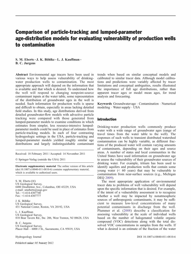
Despite many and varied applications of environmentaltracer analysis and modeling to characterize groundwaterages in aquifers and watersheds, direct comparisons ofage distribution results from distributed- and lumped-parameter models for drinking-water production wells ornatural groundwater discharge are relatively limited (e.g.,Scanlon et al. 2003). The purpose of this paper is tocompare (1) the ability of the different models to matchobserved tracer concentrations in a typical productionwell in each of several contrasting hydrogeologic settings,and (2) predicted responses at the wells to a change innonpoint-source contaminant input based on the simulatedage distributions. The field sites are located within fouraquifer systems, which together supplied 35% of thewater used for public supply in the United States in 2000(Maupin and Barber 2005): Modesto, California (CentralValley aquifer system); Tampa, Florida (Floridan aquifersystem); Woodbury, Connecticut (Glacial aquifer system);and York, Nebraska (High Plains aquifer) (Fig. 1 andTable 1; Eberts et al. 2005). The model approaches are:distributed-parameter groundwater-flow models with ad-vective particle tracking (Harbaugh et al. 2000; Pollock1994) and lumped-parameter models, including the linearmodel (L), the exponential model (E), the exponentialpiston-flow model (EP), and the dispersion model (DM)of Maloszewski and Zuber (1982, 1993). In addition, twobinary mixing models (BEP, BPP) involving younger andolder components with differing age distributions wereapplied (Table 1). All models were calibrated usinginverse methods to multiple environmental-tracer meas-urements. The distributed-parameter flow models summa-rized herein have been described previously (Burow et al.2008; Crandall et al. 2009; Starn and Brown 2007; Clarket al. 2007), whereas the lumped-parameter models andcomparisons are new. Discussions focus on the utility ofthe different approaches for informing source-waterprotection decisions and assessing production-well vul-nerability to nonpoint-source contamination. The differentfield sites illustrate differences in the complexity of theapproaches and sensitivity of the results in someimportant types of aquifer settings.

Hydrogeologic settings

The Modesto, California study area has a semiarid climateand receives an average of 315 mm of precipitation peryear. Irrigation in the agricultural area just outside ofModesto has increased groundwater recharge rates to


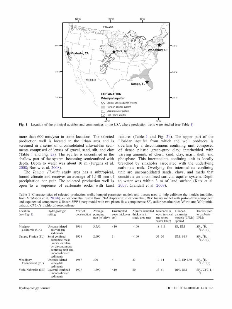
more than 600 mm/year in some locations. The selectedproduction well is located in the urban area and isscreened in a series of unconsolidated alluvial-fan sedi-ments comprised of lenses of gravel, sand, silt, and clay(Table 1 and Fig. 2a). The aquifer is unconfined in theshallow part of the system, becoming semiconfined withdepth. Depth to water was about 10 m (Jurgens et al.2008; Burow et al. 2008).

The Tampa, Florida study area has a subtropical,humid climate and receives an average of 1,140 mm ofprecipitation per year. The selected production well isopen to a sequence of carbonate rocks with karst

features (Table 1 and Fig. 2b). The upper part of theFloridan aquifer from which the well produces isoverlain by a discontinuous confining unit composedof dense plastic green-gray clay, interbedded withvarying amounts of chert, sand, clay, marl, shell, andphosphate. This intermediate confining unit is locallybreached by sinkholes associated with the underlyingcarbonate rock. Overlying the intermediate confiningunit are unconsolidated sands, clays, and marls thatconstitute an unconfined surficial aquifer system. Depthto water was within 3 m of land surface (Katz et al.2007; Crandall et al. 2009).

Fig. 1 Location of the principal aquifers and communities in the USA where production wells were studied (see Table 1)

Table 1 Characteristics of selected production wells, lumped-parameter models and tracers used to help calibrate the models (modifiedfrom McMahon et al. 2008b). EP exponential piston flow; DM dispersion; E exponential; BEP binary model with piston-flow componentand exponential component; L linear; BPP binary model with two piston-flow components; SF6 sulfur hexafluoride;

3H tritium; 3H(0) initialtritium; CFC-11 trichlorofluoromethane

Location(see Fig. 1)

Hydrogeologicsetting

Year ofconstruction

Averagepumpingrate (m3/day)

Unsaturatedzone thickness(m)

Aquifer saturatedthickness instudy area (m)

Screened oropen interval(m belowwater table)

Lumped-parametermodels (LPMs)applied

Tracers usedto calibrateLPMs

Modesto,California (CA)

Unconsolidatedalluvial-fansediments

1961 3,750 <10 >100 18–111 EP, DM SF6,3H,

3H/3H(0)

Tampa, Florida (FL) Semi-confinedcarbonate rocks(karst); overlainby discontinuousconfining unit andunconsolidatedsediments

1958 2,690 3 >100 33–50 DM, BEP SF6,3H,

3H/3H(0)

Woodbury,Connecticut (CT)

Unconsolidatedvalley-fillsediments

1967 390 4 23 10–14 L, E, EP, DM SF6,3H,

3H/3H(0)

York, Nebraska (NE) Layered, confinedunconsolidatedsediments

1977 1,390 <10 80 33–61 BPP, DM SF6, CFC-11,3H


The Woodbury, Connecticut study area has a humidclimate and receives an average of 1,170 mm ofprecipitation per year. The selected production well isscreened in stratified unconsolidated glacial deposits in thePomperaug River valley (Table 1 and Fig. 2c). The Glacialaquifer system is locally unconfined and depth to waterwas about 4 m. The unconsolidated valley-fill sedimentsare underlain by granite, quartzite, schist, and gneiss(Brown et al. 2009; Starn and Brown 2007).

The York, Nebraska study area has a humid, continen-tal climate and receives an average of 711 mm ofprecipitation per year. The selected production well isopen to the uppermost confined aquifer in a layeredsequence of gravels, sands, silts, and clays (Table 1 andFig. 2d). The confining unit that separates this aquiferfrom the overlying unconfined aquifer ranges in thicknessfrom 8 to 17 m and is laterally continuous. Both aquifersare heavily utilized for irrigation, with approximately 2wells per km2, and many irrigation wells are screenedacross the confining unit. Depth to water in the unconfinedaquifer was within 10 m of land surface (Landon et al.2008; Clark et al. 2007).

Methods

General approachGeochemical, isotopic, and environmental age tracer datawere obtained from the representative drinking-waterproduction well and several nearby short-screened moni-toring wells in each study area during 2003–2006. Themonitoring-well network in each area was installed in ornear the zone of contribution of the selected production

well on the basis of regional-scale (102 to 103 km2)groundwater-flow models and advective particle tracking(Paschke et al. 2007), incorporating a grid refinementapproach (Spitz 2001). Analyzed environmental tracersincluded various combinations of sulfur hexafluoride(SF6), chlorofluorocarbons (CFCs), tritium (3H), andtritiogenic helium-3 (3He*), depending on the setting.Because of anticipated effects of wellbore mixing ongroundwater age distributions, multiple environmental agetracers were analyzed for each sample, and additionalisotopic and chemical data were used to detect reactionsand mixing of water masses (Katz et al. 2007; Jurgens etal. 2008; Landon et al. 2008; Brown et al. 2009). Noblegas and nitrogen gas data were used to estimate rechargetemperatures and excess air concentrations to convertmeasured concentrations of the atmospheric environmen-tal tracers in the water samples to concentrations in air forcomparison to historical atmospheric concentrations(Plummer et al. 2001). Graphical inspection of data(comparing individual tracers to each other and to simplemixing models) provided initial screening for samplesexhibiting tracer contamination or degradation and wasused to help select the most appropriate data for inversemodeling of groundwater-age distributions.

Both modeling approaches (particle-tracking andlumped-parameter) were based on the assumption thatindividual non-reacting environmental tracers and non-point-source contaminants were transported with watermolecules (e.g., solutes and solvent were not fractionatedfrom each other by differential diffusion). Therefore, inboth model approaches, regardless of the complexity ofthe hydrologic conceptualization, the concentration of atracer in a particle was a function of the age of the particle

Fig. 2 Conceptual hydrogeologic models of the investigated areas in a Modesto, California, b Tampa, Florida, c Woodbury, Connecticut,and d York, Nebraska. Red arrows: precipitation (input), blue arrows: groundwater flow, purple arrows: groundwater abstraction (output),blue dashed line: water table. Modified from Landon et al. 2006


and the input history of the tracer. The simulated flux-weighted tracer concentration in a mixed sample from agiven well at a particular sample date was approximatedby a numerical non-parametric version of the convolutionintegral:

Cs;ts ¼ S Xi;ti � Ci;ti � exp �l � ti½ �� ð1Þwhere Cs,ts is the concentration of a tracer in a sample (s)at the time (date) when the sample was collected foranalysis (ts), Xi,τi is the fraction of the total sampleconsisting of groundwater with a particular age (C i), Ci,ti isthe concentration of a tracer in a fraction of the watersample at the time (date) when that fraction entered thesystem (ti= ts - C i), 1 is a first-order decay constant (zerofor a stable tracer), and the sum is over all yearsrepresented in the sample (ΣXi,τi=1.0). All particle-tracking and lumped-parameter models were calibratedto tracer data by adjusting selected model parametervalues until the best match was achieved betweensimulated tracer concentrations—derived from computedage distributions using Eq. 1—and measured concentra-tions for the tracers.

To explore differences between the models and theirability to predict contaminant responses in each produc-tion well, computed age distributions were applied to ahypothetical slug input of a conservative contaminantentering the aquifer across the entire area contributingrecharge and lasting 25 years. Selected characteristics ofthe breakthrough curves from the particle-tracking andlumped-parameter models for each well were compared todetermine which, if any, of the model differences notablyaffect contaminant predictions. In addition, results frompiston-flow models calibrated to tracer data from eachproduction well were graphed to help illustrate theimportance of full age distributions, rather than apparenttracer ages or model mean ages, for trend analysis andforecasting.

Sample collection and data evaluationWater samples were collected using protocols in Koterbaet al. (1995) and analyzed for a broad suite of constituentsthat could be used to determine water sources andreactions affecting the chemical composition of thegroundwater in each setting (Katz et al. 2007; Jurgens etal. 2008; Landon et al. 2008; Brown et al. 2009). Samplesfrom the production wells were collected near thewellhead by means of sample tubing connected to astainless-steel ball valve that tapped the discharge pipebefore the water was chlorinated or treated in any way.Sulfur hexafluoride samples were collected by placing thesampling discharge tubing in the bottom of the samplebottle and displacing the air in the bottle with groundwa-ter. After approximately 2 L of overflow, the sampling linewas removed. The bottles were capped with polysealconical screw-caps without headspace. Chlorofluorocar-bon samples were collected by inserting the end of the

discharge tubing into the bottom of a 125-ml glass bottle,allowing at least 2 L to overflow into a 2-L beaker, thencapping the sample bottle with an Al foil-lined cap underwater within the beaker. Tritium samples were collected in500-ml bottles for determination by 3He in-growth.Samples for helium (He) and neon (Ne) analyses anddetermination of the 3He/4He isotope ratio (δ3He) ofdissolved He were collected in crimped copper tubes.Samples for additional dissolved gases (N2, Ar, CO2, CH4,O2) were collected in 160 mL serum bottles, which weresealed in a large beaker under flowing well water.

Concentrations of SF6 and CFCs were determined atthe US Geological Survey (USGS) CFC laboratory inReston, Virginia, using purge and trap, gas-chromatographictechniques with electron-capture detector (GC-ECD;Busenberg and Plummer 1992, 2000). Concentrations of3H, He, Ne, and 3He/4He were determined at the NobleGas Laboratory of Lamont-Doherty Earth Observatory inPalisades, New York, using methods described in Clarket al. (1976), Bayer et al. (1989), and Solomon et al.(1992). Some 3H concentrations were determined at theUSGS Noble Gas Laboratory in Denver, Colorado, usingsimilar methods. Some major dissolved gas analyses alsowere obtained from the USGS Noble Gas Lab. Thesesamples were extracted on an ultra-high vacuum extrac-tion line; the extracted gas was analyzed for N2, O2,CH4, and Ar using a quadrapole mass spectrometer indynamic operation mode. Noble gas isotopic concen-trations and compositions were measured using separatealiquots on a magnetic sector mass spectrometer whichwas run in static operation mode. Concentrations ofdissolved gases (N2, O2, CH4, Ar, and CO2) for allremaining samples were determined at the USGS CFClaboratory by gas chromatography after creation andextraction of headspace in the glass serum bottles(Busenberg et al. 1998).

Recharge temperatures and concentrations of excess airin the groundwater were calculated from the noble gasdata according to the closed-system equilibration (CE)model (Aeschbach-Hertig et al. 1999, 2000; Peeters et al.2002). Where only Ar and N2 data were available, excessair was assumed to be unfractionated (Heaton and Vogel1981). For cases where only Ar and N2 data wereavailable and the sample was anaerobic, the temperatureand excess air were assumed to be equal to the averagefrom aerobic samples in the data set for the study area.This was done because of the potential effect ofdenitrification on the measured N2 concentration in someof these samples (McMahon et al. 2008a).

Concentrations of SF6 and CFCs in water samples fromthe study wells were converted to equilibrium concen-trations in air (as dry air mixing ratios, in parts per trillionby volume, pptv) using the calculated recharge temper-atures and excess air content for the samples, so thatconcentrations in the water samples could be comparedwith historic air mixing ratios for the compounds(Busenberg and Plummer 2000; Plummer and Busenberg2000). Concentrations of 3He* in water samples collectedfrom the study wells were determined from mass balance


equations for 3He and 4He, using the measured He, Ne, and3He/4He ratio for a sample, the calculated recharge temper-ature, and an assumed 3He/4He ratio of terrigenic He(Schlosser et al. 1989; Solomon et al. 1992; Solomon andCook 2000). All samples were evaluated for terrigenicsources of He and adjusted accordingly. The concentrationof initial 3H (3H(0), tritium concentration before decay) wascomputed as the concentration of 3H plus the concentra-tion of 3He* in each sample. When comparing simulatedconcentrations with these measurement-based concentra-tions, both 3H and 3H(0) were simulated as independenttracers (Eq. 1), assuming the decay product (3He*) movedwith the 3H in each simulated particle. Subsequently, theratio of 3H/3H(0) was computed for mixed samples fromthe simulated values of 3H and 3H(0) in the mixtures.Details of the SF6, CFC, and

3He* calculations as well asan evaluation of the uncertainty associated with themeasurements and calculations are given in Katz et al.(2007), Jurgens et al. (2008), Landon et al. (2008), andBrown et al. (2009). The term “measured concentrations”from this point forward implies measurement-basedconcentrations that have been corrected, converted, orcalculated, as discussed in the preceding.

Atmospheric input records for SF6 and CFCs wereobtained from Busenberg and Plummer (2006) andPlummer and Busenberg (2006), respectively. Atmosphericinputs for 3H were estimated using a computer program(Michel 1989) that interpolates 3H concentrations fromlatitude-longitude data in the continental US usingmeasurements from available long-term monitoring sta-tions; records were extended by correlation to Interna-tional Atomic Energy Agency data from Vienna, Austria(IAEA/WMO 2006).

Differences in unsaturated zone transport of 3H, whichinfiltrates as part of the water molecule and decays(“ages”) during unsaturated zone transport, and the gases(SF6, CFCs, and He), which pass through the unsaturatedzone largely in the gas phase (Cook and Solomon 1995),were not explicitly considered. All of the study areas hadunsaturated zone thicknesses of ≤10 m and (or) high ratesof recharge (discussed in the preceding), such that traveltimes through the unsaturated zone were considered to berelatively small, and not much larger than the uncertaintiesof the age distributions for the wells.

Distributed-parameter groundwater-flow modelswith particle trackingSteady state, local-scale (< 15 km2) three-dimensionalgroundwater-flow models were constructed for each studyarea using MODFLOW-2000 (Harbaugh et al. 2000). TheUSGS particle tracking routine, MODPATH (Pollock1994), was used to simulate pathlines and advective traveltimes. Upwards or downwards flow within wellbores(boreholes completed as wells) that were simulated inmultiple nodes or layers in the models was tracked bymeans of the multi-node well package for MODFLOW(Halford and Hanson 2002). A combination of non-linearregression (Hill et al. 2000; Poeter et al. 2005) and trial

and error techniques was employed to calibrate the modelsto observed water levels, hydraulic gradients, streamflowgains and/or losses, and environmental tracer data fromboth the monitoring wells and production wells, asdescribed in the following. Calibration of the groundwa-ter-flow models to tracer concentrations was done byapplying Eq. 1 using flux-weighted age distributions togenerate simulated tracer concentrations for each well forcomparison with measured concentrations during errorminimization (Clark et al. 2007; Starn and Brown 2007;Burow et al. 2008; Crandall et al. 2009). Flux-weightedage distributions were obtained by delineating the areascontributing recharge to the wells using particles that werecaptured by the wells during forward tracking. The traveltime for each such particle was recorded and thevolumetric flux associated with the particle was computedby dividing the total inflow at the model cell face wherethe particle was started by the total number of particlesstarted at the same cell face. The flux data for all particlesrelated to a given production well were divided into 1-yearbins on the basis of simulated travel times to determine thefraction of the total sample consisting of water with agiven age in years (Xi,τi in Eq. 1).

The Modesto, California groundwater-flow model hada uniform grid of 200 rows of 72-m-length cells and 100columns of 34-m-length cells, and 200 layers with auniform thickness of 0.6 m, representing the thickness ofindividual hydrofacies units (Burow et al. 2008). Thespatial distribution of the hydrofacies was determinedusing borehole lithologic data and a three-dimensionalspatial correlation model of hydrofacies developed usingthe program T-PROGS (Carle et al. 1998; Carle 1999).The steady-state model simulated aquifer stresses thatexisted in water year 2000 and included pumping at 22production wells. A preliminary calibration was carriedout using the parameter estimation process in MODFLOW-2000 (Hill et al. 2000). Because of difficulty updatinghydraulic-conductivity-weighted flux boundaries duringeach parameter estimation run, and because of parametercorrelation, estimates for the hydraulic conductivityparameters were later refined using a systematic manual-calibration approach. Observations included water levelsmeasured in 18 monitoring wells screened at multipledepths from 2003 to 2005. Longer-term water-leveland pumping data indicated that climatic conditionsdid not change significantly between 2000 (when thepumping data were collected) and 2005 (when the lastof the water-level data were collected). Measured SF6concentrations in 8 wells and 3H concentrations in 20wells from October 2003 and November 2004 wereused to help calibrate this distributed-parameter model(Burow et al. 2008; Jurgens et al. 2008).

The Tampa, Florida groundwater-flow model had auniform grid of 125-m-length cells (80 rows, 69 columns)and 13 layers of variable thickness (Crandall et al. 2009).The steady-state flow model simulated average annualconditions for calendar year 2000 and included pumpingfrom 77 production wells. Karst features such as closed-basin depressions, preferential flow along fractures, and


conduit features were incorporated into the model usinghigh vertical hydraulic conductivity, high recharge, andlow porosity values where such features were identified.Twenty-four hydraulic conductivity, recharge, riverbed/drain conductance, and transport (effective porosity)parameters were used to represent the groundwater-flowsystem. Seventeen parameters, including hydraulic con-ductivity, recharge, and effective porosity, were estimatedusing UCODE (Poeter et al. 2005). Observations includedgroundwater levels from 30 monitoring wells and theproduction well, hydraulic gradients from 22 monitoringwell nests, and measured concentrations of SF6 and 3Hfrom 17 monitoring wells and the production well. Theenvironmental tracer data used to help calibrate thisdistributed-parameter model were collected betweenDecember 2003 and August 2005 (Katz et al. 2007;Crandall et al. 2009).

The Woodbury, Connecticut groundwater-flow modelhad a uniform grid of 15.2-m-length cells (241 rows, 322columns), 7 layers of variable thickness, and simulatedaverage annual conditions approximated during 1997–2001, including pumping at five production wells (Starnand Brown 2007). Model parameter values were estimatedusing the parameter estimation process in MODFLOW-2000. Observations included water levels in 34 monitoringwells and estimates of streamflow gains and/or losses fromstreamflow data. Simulated travel times were compared topiston-flow model 3H/3He ages (as opposed to tracerconcentrations) for 13 of the monitoring wells and theproduction well; apparent 3H/3He ages were less affectedby mixing at this site than at the other sites because theage of nearly all groundwater at the Woodbury site wasrelatively young (generally <10 years), and the wellscreens were relatively short (< 4 m in length). In addition,simulated and measured 3H concentrations were comparedfor the production well. The environmental tracer dataused to help calibrate this distributed-parameter modelwere collected between November 2003 and August 2004(Starn and Brown 2007; Brown et al. 2009).

The York, Nebraska groundwater-flow model had auniform grid of 40.2-m-length cells (180 rows, 372columns) and 14 layers of variable thickness (Clark et al.2007). A transient model that simulated groundwater flowfor a 60-year period and included pumping from 183production wells was initially constructed and manuallycalibrated to 470 water-level measurements from 53 wells.A transport model within a sub-grid of the groundwaterflow model was created with MODFLOW-GWT (Konikowet al. 1996; Konikow and Hornberger 2006) and used torefine the model calibration. Parameter values (horizontalhydraulic conductivity, vertical anisotropy, specific yield,specific storage, porosity) were manually adjusted tominimize differences between groundwater ages computedusing the transport model following methods by Goode(1996) and apparent (piston-flow model) 3H/3He and CFC-11 ages for unconfined aquifer monitoring wells with shortscreens. Simulated CFC-11 concentrations for confinedaquifer monitoring wells and the production well werecompared to measured concentrations for the same wells.

The simulated CFC-11 concentrations were computed usinga steady-state model representing average annual stresses forthe period 1997–2001, which was derived from the transientmodel. The environmental tracer data used to help calibratethis distributed-parameter model were collected betweenOctober 2003 and October 2005 (Clark et al. 2007; Landonet al. 2008).

Lumped-parameter modelsSteady-state lumped-parameter models (LPMs) were usedto describe measured tracer concentrations in each studyarea. The lumped-parameter modeling approach appliedherein was fundamentally similar to the particle-trackingapproach except that values of Xi,τi in Eq. (1) werecomputed from conceptually relevant weighting functions(analytic age-distribution models) rather than beingderived from collections of simulated particles and theirtransit times. An important difference between theapproaches is that the lumped-parameter models treatedthe flow system as a whole, or as relatively few discretecomponents, and were calibrated using only environmen-tal tracer data from the production well of interest,whereas the particle-tracking models included spatialvariations in aquifer hydraulic and chemical propertiesand were calibrated using multiple types of data from theproduction well and monitoring wells.

The weighting functions for the linear model (L), theexponential model (E), the exponential piston-flow model(EP), and the dispersion model (DM) that were applied inthis study are presented in Maloszewski and Zuber (1982).The L model is relevant for production wells completed inan unconfined wedge-shaped aquifer or other situations inwhich age increases linearly with depth. Mean age of themixed sample (Cs, subsequently referred to as τ or tau) isthe only model parameter. The E model is relevant forproduction wells in which the shortest flowpath has atravel time equal to zero, the longest has a travel timeequal to infinity, and the intervening flowpaths have traveltimes that are distributed exponentially (decreasing Xi,τifrom young to old). Mean age of the sample (C ) is the onlymodel parameter. In the EP model, the aquifer is assumed toconsist of two components of groundwater flow in series,one component described by the exponential model (E) andanother component described by the piston-flow model (P)in which all flowpaths are assumed to have the same traveltime. The EP model can be used to describe discharge froman aquifer of constant thickness with an upgradientunconfined portion receiving areally distributed recharge(the E part) connected to a downgradient confined portion oran unconfined portion receiving little to no recharge (the Ppart). Parameter values are the mean age of the sample (C )and a ratio that describes the relative contributions of the Pand E components to the overall mean age, xP/xE, where xEcould be equal to the horizontal distance along the flowpathcontributing to recharge and xP the horizontal distance alongthe flowpath not receiving recharge (Cook and Böhlke2000). The EP model can also be used to describe the agemixture at a well in which the screened interval does not


extend all the way up to the water table and the youngest partof an exponential age distribution in the surrounding aquiferis not sampled by the well. For a well screened from thebottom of the aquifer up to an arbitrary depth below thewater table, the parameter xP/xE can be replaced by anexpression relating the relative heights of the screened andunscreened portions of the well (assuming the aquifer has anexponential age distribution) (Vogel 1967; Cook and Böhlke2000):

xP=xE ¼ �ln 1� z=Zð Þ ð2Þwhere z is the distance from the water table to the top ofthe screened interval and Z is the total saturated thicknessof the aquifer. The DM model approximates the agedistribution caused by longitudinal dispersion wheregroundwater particles with different travel times coexistin close proximity. Parameters for this model includemean age (C ) and a dispersion parameter (D’).

The binary mixing models used in this study describesituations in which two different water masses fromparallel reservoirs mix in a production well. The firstbinary mixing model (BPP) describes mixing between twocomponents with discrete ages and tracer concentrations.In this study, the BPP model was applied to situations inwhich relatively young tracer-bearing water with adiscrete age mixed with relatively old, tracer-free water.Independent parameters for the BPP model are the meanage of the mixture (C ), the age of the young component,and the age of the old component. The age of the oldcomponent was fixed at 60 years to represent tracer-freewater. Consequently, the mean age of the mixture is aminimum value as the true age of any tracer-freecomponent is not known and could be large. In contrast,the mean age of the young component and the fractionalcontribution of this component are meaningful. Thesecond binary mixing model (BEP) describes mixingbetween a component with an exponential distribution ofages (E) and a component with a discrete age (P) that isyounger than that of the exponential component. In thisstudy, the BEP model was applied to a karst situation inwhich very young water that travels along conduit featuresmixes in a production well with water from the rockmatrix. Parameters for the BEP model are mean age of themixture (C ), mean age of the exponential component, andage of the piston-flow component.

The Excel workbook TRACERMODEL1 (Böhlke2006) was updated to include the DM, BPP and BEPmodels and used to solve Eq. (1) for each model that wasevaluated for a given production well. After models withconceptual relevance to the production well and localhydrogeologic setting were selected for comparison, amulti-step approach was used to estimate the modelparameter values. Initial parameter values were deter-mined by comparing measured tracer concentrations withconcentrations corresponding to model age distributionson tracer-tracer graphs (where curves indicate all combi-nations of tracer concentrations consistent with a givenmodel type but varying mean age) and tracer-time graphs

(where curves indicate concentrations of individual tracersin a well over time, for a given model type and mean age).Initial values for parameters that affect the plottingpositions of model curves on tracer-tracer graphs (e.g.,D’ for DM; and C of both components for BPP and BEP)were determined first, by manually adjusting parametervalues to obtain a match between the model curve and thetracer data for the production well. For the xP/xEparameter of the EP model, which also affects the plottingposition of model curves on tracer-tracer graphs, initialvalues were determined in some cases using informationon the screened and unscreened portions of the well (e.g.,Modesto, using Eq. 2, as described in the Results anddiscussion section in the following). Initial values forparameters that do not affect plotting position on tracer-tracer graphs but do affect plotting position on tracer-timegraphs (e.g., C for E, EP and DM) were then selected in asimilar way. Finally, Excel Solver (Fylstra et al. 1998) wasused to optimize the parameter values for each model byminimizing the mean absolute percentage error (MAPE) ofmeasured and simulated tracer concentrations. This errorfunction assigns an equal weight to each tracer so that tracerswith different units were not preferentially optimized:

MAPE ¼ 1

n

Xni¼1

100Mi � SiMi

� �� ð3Þ

where Mi is the measured value, Si is the simulated value,and n is the number of tracers used in the fit. Carefulselection of initial parameter values, and multiple trials,were used to avoid local minima. A new Excel workbook,TracerLPM (Jurgens BC, Böhlke JK, Eberts SM, USGeological Survey, unpublished report “TracerLPM: AnExcel® Workbook for interpreting groundwater age fromenvironmental tracers”, 2011), also was applied and gavesimilar results.

Because the production wells were sampled more thanonce (Table 2), dates for model curves plotted on tracer-tracer graphs (see electronic supplementary material ESM)were calculated for average sample dates at each site(typically±1–2 years), although curves for all sampledates were created and evaluated. Tracer-time graphs(ESM) were used to compare measured tracer concen-trations with simulated concentrations from both lumped-parameter and particle-tracking models for each produc-tion well and sampling date.

Results and discussion

Modesto, California, unconsolidated alluvial-fansediments

Modesto inverse modelsTracer data and model results for the Modesto site aresummarized in Tables 2 and 3, Fig. 3a, and ESM figures 1and 2 in the electronic supplementary material (ESM).The long screened interval of the Modesto production well


(> 90 m) combined with strong, downward hydraulicgradients within the aquifer (up to 0.3) resulted indownward flow of water within the well when it was notpumping. Evidence for this downward movement of waterincluded seasonal fluctuations in nitrate and uraniumconcentrations in the well, which occurred becauseshallow contaminated water moved into deeper parts ofthe aquifer near the wellbore during periods of low or nopumping and subsequently was pulled back out whenpumping resumed (greatest during winter months whendown time between pumping events was longest) (Burowet al. 2008; Jurgens et al. 2008). This intra-wellbore flowhad the potential to affect concentrations of environmentaltracers and, to a lesser extent, ratios of tracers. Thus, datacollected during the summer pumping season were mostrepresentative of the surrounding aquifer system (Table 2)and the timing of tracer data collection was a considerationfor estimating the age distribution of water from this well.

Lumped-parameter models applied to the Modesto siteincluded the EP and DM models. For the EP model, theinitial estimate of the xP/xE parameter (0.18) wascomputed from the length of the saturated cased intervalbelow the water table (18 m) and the total length of thewell including the screened interval (111 m) using Eq. 2.For the DM model, the initial estimate for the D’parameter was obtained by adjusting the parameter valueuntil the model curve best matched the selected tracer dataon tracer-tracer graphs (see ESM figure 1, ESM). The finalEP (C =54; xP/xE=0.2) and DM (C =59; D’=0.51) modelswere both conceptually feasible and reproduced theproduction-well tracer data from August 2004 and August2006—times when the effects of intra-wellbore flow ontracer concentrations were likely to be minimal (see ESMfigures 1 and 2, ESM).

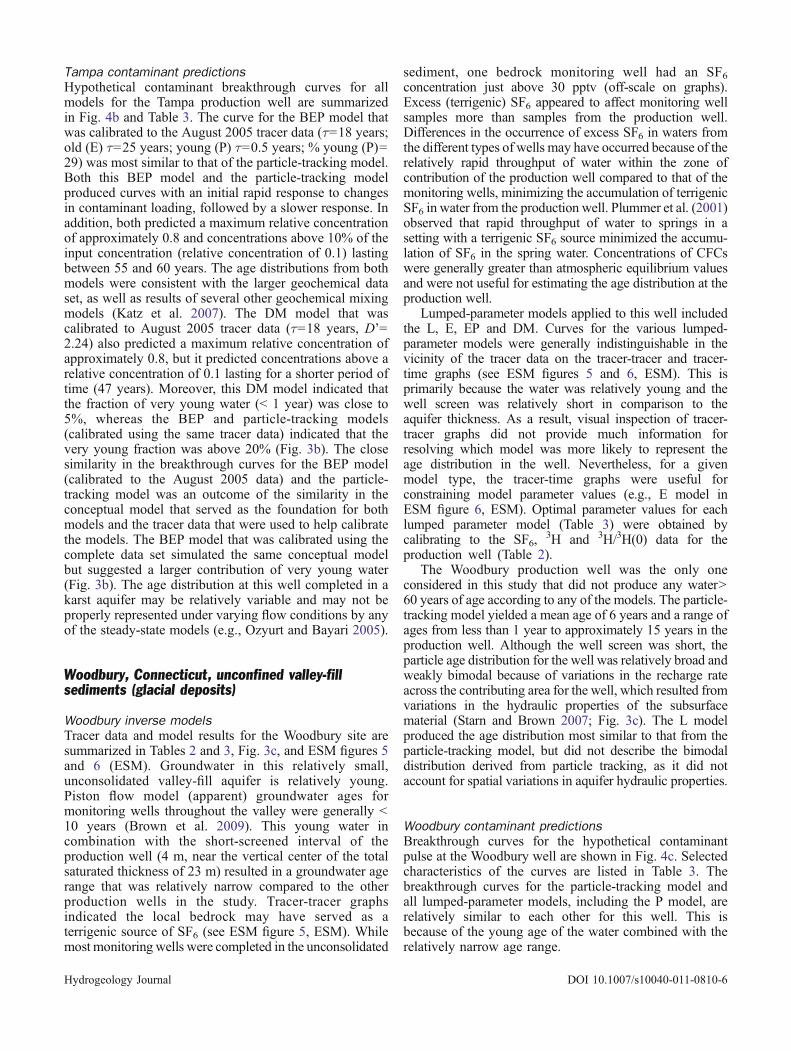
Water samples from the Modesto well had a wide rangeof ages minus the youngest fraction that was missingbecause the top of the well screen was 18 m below thewater table. The particle-tracking model yielded an agerange for the well of 9 years to more than 1,000 years. Thesimulated peak in the age distribution from this model wasaround 25 years (Fig. 3a) (Burow et al. 2008). Graphs of3H versus 3H/3H(0) and of SF6 versus 3H/3H(0) confirmthat the water from the production well is of mixed age—the tracer data plot off curves that describe no mixing (seeESM figure 1, ESM). This was not unexpected for theproduction well because of its long screened interval. Thesame was also true, however, for samples from nearbymonitoring wells (1.5-m screened intervals), which isconsistent with other modeling studies indicating aquiferheterogeneity can affect apparent SF6 ages in short-screenwells in the California Central Valley (Weissmann et al.2002; Green et al. 2010). The large difference between themean age calculated using the particle-tracking model(420 years) and the mean ages calculated using the twolumped-parameter models (54 and 59 years) illustrateshow small numbers of very old particles can influence themean age computed from particle-tracking results. Themedian age from the particle-tracking was 46 years.

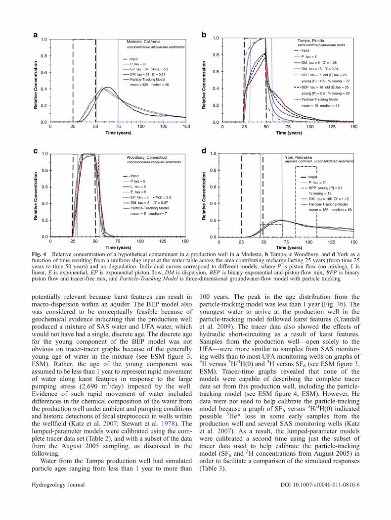
Modesto contaminant predictionsBreakthrough curves for the Modesto production wellbased on the age distributions from each of the calibratedmodels and a hypothetical nonpoint-source contaminantwith a uniform input at the water table lasting 25 yearsand without degradation are plotted on Fig. 4a and furthercharacterized in Table 3. The particle-tracking modelpredicted a maximum relative concentration of 0.43,

Table 2 Environmental tracer data for samples from selected production wells. Data for Modesto, Tampa, Woodbury, and York prior to2006 from Jurgens et al. (2008), Katz et al. (2007), Brown et al. (2009), and Landon et al. (2008), respectively (ND no data)

Sample date SulfurhexafluorideSF6 (pptv

a)

Trichlorofluoro-methane CFC-11(pptv)

Tritium 3H (TUb) Tritiogenic helium-33He* (TU)

Initial tritiumc

3H(0) (TU)Tritium/ initialtritium 3H/3H(0)

Modesto, CaliforniaNov-2003 ND ND 6.88d 41.40d 48.28d 0.14d

Aug-2004 0.73 ND 4.57 32.70d 37.27d 0.12Aug-2006 0.88 ND ND ND ND NDTampa, FloridaJan-2004 ND ND 2.21 ND ND NDOct-2004 ND ND 2.10 0.36d 2.46d 0.85Aug-2005 3.81 ND 2.17 ND ND NDJul-2006 5.40 ND 2.01 0.56d 2.57d 0.78Woodbury, ConnecticutDec-2003 4.76 ND 6.76 2.98d 9.74d 0.69Aug-2004 4.43 ND 6.80 2.46d 9.26d 0.73Jul-2006 5.44 199.0d ND ND ND NDYork, NebraskaOct-2003 0.24 38.1 0.60 ND ND NDJun-2004 0.27 ND 0.61 110.79d 111.40d 0.01d

Aug-2006 0.30 48.8 ND ND ND ND

a Parts per trillion by volume. Concentrations corrected for excess airb Tritium unitc3 H+3He*dData not used for lumped-parameter model calibration


Table 3 Model parameter values and breakthrough-curve characteristics at production wells for a hypothetical contaminant with a uniformslug input at the water table lasting 25 years and no degradation. Median age, peak lag time, dilution at peak, arrival: 1% of total mass, andflush: 99% of total mass for Particle-Tracking Models are from McMahon et al. (2008b) (EP exponential piston-flow model; DM dispersionmodel; BEP binary model with piston-flow component and exponential component; L linear model; E exponential model; BPP binarymodel with two piston-flow components; PTM particle-tracking model)

Model Meanabsolutepercentageerror (%)

Peak lagtimea (years)

Dilutionat peak(C/Co)

b

Arrival: 1%of total massc

(years)

Flush: 99%of totalmassd (years)

Time to breach10% of inputconcentrationc

(C/Co=0.1) (years)

Time to returnto below 10% ofinput concentrationc

(C/Co=0.1) (years)

Time above10% of inputconcentration(C/Co=0.1)(years)

Modesto, CaliforniaEP taue=54 years,xP/xE=0.2

7.5 20 0.43 14 205 13 99 86

DMf tau=59 years,D'=0.51

7.6 22 0.40 14 275 14 94 80

PTM mean age=420years, medianage=46 years

19.5g 26 0.43 17 216 18 78 60

Tampa, FloridaDMh tau=6 years,D'=1.06

14.7 12 1.00 2 30 <1 37 37

DMi tau=18 years,D'=2.24

0.3 12 0.82 2 164 1 48 47

BEPh tau=7 years,old (E) tau=25 years,young (P)=0.5 years,% young (P)=72

10.2 12 0.99 1 16 <1 32 32

BEPi tau=18 years,old (E) tau=25 years,young (P)=0.5 years,% young (P)=29

9.2 12 0.82 1 68 <1 55 55

PTM mean age=15years, medianage=13 years

41.8g 12 0.76 2 61 <1 60 60

Woodbury, ConnecticutL tau=6 years 4.5 <1 1.00 2 9 1 35 34E tau=5 years 4.1 12 1.00 2 13 <1 35 35EP tau=5 years,xP/xE=2.8

4.2 11 1.00 5 7 4 32 28

DM tau=5 years,D'=0.37

3.3 12 0.98 3 14 1 35 34

PTM mean age=6 years, medianage=7 years

5.0g 6 1.00 3 8 1 33 32

York, NebraskaBPP old (P) tau≥60years, young(P)=21 years,% young (P)=15

10.0 21j 0.15j 21 ≥60 21 46j 25j

DM tau=180 years,D'=1.12

66.0 28 0.21 18 322 23 98 75

PTM mean age=186 years, medianage=80 years

222.0g 30 0.20 18 359 25 122 97

a Time lag between input midpoint of 12.5 years and first occurrence of peak concentrationb Concentration relative to input concentrationc Time relative to start of inputd Time relative to end of inpute tau refers to mean agef Dispersion model parameters follow Maloszewski and Zuber (1982)gMean absolute percentage error for PTMs computed from measured and simulated tracer concentrations at the production well forcomparison purposes only. PTMs were calibrated to a variety of distributed data, including water levels, hydraulic gradients,streamflow gains and/or losses, and environmental tracer data for both monitoring wells and production wells. Consequently, tracerdata for individual production wells have less influence on PTM model calibration than they do on lumped-parameter modelcalibrationh Calibrated to data from January 2004, October 2004, August 2005, and July 2006i Calibrated to data from August 2005j Young fraction only


whereas the maximum relative concentration would havebeen 1.0 had there been no mixing (P model). The EP andDM predicted maximum relative concentrations of 0.43 and0.40, respectively. Both the EP and DMmodels predicted thearrival of the first 1% of total mass at the well within 3 yearsof the particle tracking predictions. An important feature ofthe EP, DM and particle-tracking models is the delay beforecontaminant arrival and recovery caused by the lack ofyoung water, owing to the distance between the water tableand the top of the well screen. The models all predictsomewhat different flushing times for the last 1% of totalmass and different amounts of time above a thresholdconcentration equal to 10% of the input concentration(relative concentration of 0.1; Table 3). The small fractionof water produced by this well that is young enough tocontain the selected age tracers contributes to the relativelylarge uncertainties in the tail end of the age distributions fromthe fitted models (Zuber et al. 2005; Chorco Alvarado et al.2007). Had tracers of much older groundwater such ascarbon-14 or 4He, been included in the analysis, the tail endof the age distribution may have been better constrained.Nevertheless, all mixing models predict that concentrationswould remain above a relative concentration of 0.1 fordecades longer than the 25 years of the slug input.

Tampa, Florida, semi-confined carbonate rocks(karst)

Tampa inverse modelsTracer data and model results for the Tampa site aresummarized in Tables 2 and 3, Fig. 3b, and ESM figures 3and 4 (ESM). Karst features enabled surficial aquifersystem (SAS) water to short-circuit the intermediateconfining unit (ICU) and rapidly reach the productionwell in the Upper Floridan aquifer (UFA; Stewart et al.1978; Katz et al. 2007). Evidence indicating hydraulicshort-circuiting included concentrations of natural com-pounds (radon-222, uranium, arsenic, dissolved organiccarbon, and hydrogen sulfide) in water from the produc-tion well that were intermediate between concentrations inwater from SAS and relatively isolated UFA monitoringwells, along with concentrations of anthropogenic com-pounds (nitrate, volatile organic compounds, and pesti-cides) that were closer to those found in SAS monitoringwells. Thus, hydraulic short-circuiting by means of karstfeatures was a consideration for estimating the agedistribution of water from this well.

Lumped-parameter models applied to this well includedthe DM and BEPmodels. The DMmodel was thought to be

0.00

0.01

0.02

0.03

0 50 100 150 200

Fra

ctio

n o

f Sam

ple

Time (years)

unconsolidated alluvial-fan sediments

EP tau = 54 xP/xE = 0.2

DM tau = 59 D' = 0.51

Particle-Tracking Model

mean = 420 median = 46

0.0

0.2

0.4

0.6

0.8

02010

Fra

ctio

n o

f S

amp

le

Time (years)

semi-confined carbonate rocks

DM tau = 6 D' = 1.06

DM tau = 18 D' = 2.24

BEP tau = 7 old [E] tau = 25

young [P] = 0.5 % young = 72


young [P] = 0.5 % young = 29



0.0

0.1

0.2

0.3

0.4

0.5

02010

Fra

ctio

n o

f S

amp

le

Time (years)

unconsolidated valley-fill sediments

L tau = 6

E tau = 5

EP tau = 5 xP/xE = 2.8

DM tau = 5 D' = 0.37


mean = 6 median = 7

0.00

0.01

0.02

0 50 100 150 200

Fra

ctio

n o

f S

amp

le

Time (years)

layered, confined unconsolidated sediments

BPP young [P] = 21 % young = 15

DM tau = 180 D' = 1.12



Tampa, Florida

Woodbury, Connecticut York, Nebraska

Modesto, California a b

c d

Fig. 3 Simulated groundwater-age distributions for a Modesto, b Tampa, c Woodbury, and d York. Individual curves correspond todifferent models, where L is linear, E is exponential, EP is exponential piston flow, DM is dispersion, BEP is binary exponential and piston-flow mix, BPP is binary piston flow and tracer-free mix, and Particle-Tracking Model is three-dimensional groundwater-flow model withparticle tracking. Note that the y-axis scales are different in a–d and that the x-axis scales in b and c differ from those in a and d


potentially relevant because karst features can result inmacro-dispersion within an aquifer. The BEP model alsowas considered to be conceptually feasible because ofgeochemical evidence indicating that the production wellproduced a mixture of SAS water and UFA water, whichwould not have had a single, discrete age. The discrete agefor the young component of the BEP model was notobvious on tracer-tracer graphs because of the generallyyoung age of water in the mixture (see ESM figure 3,ESM). Rather, the age of the young component wasassumed to be less than 1 year to represent rapid movementof water along karst features in response to the largepumping stress (2,690 m3/day) imposed by the well.Evidence of such rapid movement of water includeddifferences in the chemical composition of the water fromthe production well under ambient and pumping conditionsand historic detections of fecal streptococci in wells withinthe wellfield (Katz et al. 2007; Stewart et al. 1978). Thelumped-parameter models were calibrated using the com-plete tracer data set (Table 2), and with a subset of the datafrom the August 2005 sampling, as discussed in thefollowing.

Water from the Tampa production well had simulatedparticle ages ranging from less than 1 year to more than

100 years. The peak in the age distribution from theparticle-tracking model was less than 1 year (Fig. 3b). Theyoungest water to arrive at the production well in theparticle-tracking model followed karst features (Crandallet al. 2009). The tracer data also showed the effects ofhydraulic short-circuiting as a result of karst features.Samples from the production well—open solely to theUFA—were more similar to samples from SAS monitor-ing wells than to most UFA monitoring wells on graphs of3H versus 3H/3H(0) and 3H versus SF6 (see ESM figure 3,ESM). Tracer-time graphs revealed that none of themodels were capable of describing the complete tracerdata set from this production well, including the particle-tracking model (see ESM figure 4, ESM). However, Hedata were not used to help calibrate the particle-trackingmodel because a graph of SF6 versus 3H/3H(0) indicatedpossible 3He* loss in some early samples from theproduction well and several SAS monitoring wells (Katzet al. 2007). As a result, the lumped-parameter modelswere calibrated a second time using just the subset oftracer data used to help calibrate the particle-trackingmodel (SF6 and 3H concentrations from August 2005) inorder to facilitate a comparison of the simulated responses(Table 3).

0.0

0.2

0.4

0.6

0.8

1.0

0 25 50 75 100 125 150 0 25 50 75 100 125 150

0 25 50 75 100 125 150 0 25 50 75 100 125 150

Time (years)

unconsolidated alluvial-fan sedimentssemi-confined carbonate rocks

Input

P tau = 26

EP tau = 54 xP/xE = 0.2

DM tau = 59 D' = 0.51



0.0

0.2

0.4

0.6

0.8

1.0

Rel

ativ

e C

on

cen

trat

ion

Time (years)

Input

P tau = 8

DM tau = 6 D' = 1.06

DM tau = 18 D' = 2.24


young [P] = 0.5 % young = 72


young [P] = 0.5 % young = 29



0.0

0.2

0.4

0.6

0.8

1.0

Time (years)

unconsolidated valley-fill sediments

Input

P tau = 5

L tau = 6

E tau = 5

EP tau = 5 xP/xE = 2.8

DM tau = 5 D' = 0.37


mean = 6 median = 7

0.0

0.2

0.4

0.6

0.8

1.0

Rel

ativ

e C

on

cen

trat

ion

Rel

ativ

e C

on

cen

trat

ion

Rel

ativ

e C

on

cen

trat

ion

Time (years)

layered, confined unconsolidated sediments

Input

P tau = 21

BPP young [P] = 21

% young = 15

DM tau = 180 D' = 1.12



Modesto, California Tampa, Florida

Woodbury, Connecticut York, Nebraska

a b

c d

Fig. 4 Relative concentration of a hypothetical contaminant in a production well in a Modesto, b Tampa, c Woodbury, and d York as afunction of time resulting from a uniform slug input at the water table across the area contributing recharge lasting 25 years (from time 25years to time 50 years) and no degradation. Individual curves correspond to different models, where P is piston flow (no mixing), L islinear, E is exponential, EP is exponential piston flow, DM is dispersion, BEP is binary exponential and piston-flow mix, BPP is binarypiston flow and tracer-free mix, and Particle-Tracking Model is three-dimensional groundwater-flow model with particle tracking


Tampa contaminant predictionsHypothetical contaminant breakthrough curves for allmodels for the Tampa production well are summarizedin Fig. 4b and Table 3. The curve for the BEP model thatwas calibrated to the August 2005 tracer data (τ=18 years;old (E) τ=25 years; young (P) τ=0.5 years; % young (P)=29) was most similar to that of the particle-tracking model.Both this BEP model and the particle-tracking modelproduced curves with an initial rapid response to changesin contaminant loading, followed by a slower response. Inaddition, both predicted a maximum relative concentrationof approximately 0.8 and concentrations above 10% of theinput concentration (relative concentration of 0.1) lastingbetween 55 and 60 years. The age distributions from bothmodels were consistent with the larger geochemical dataset, as well as results of several other geochemical mixingmodels (Katz et al. 2007). The DM model that wascalibrated to August 2005 tracer data (τ=18 years, D’=2.24) also predicted a maximum relative concentration ofapproximately 0.8, but it predicted concentrations above arelative concentration of 0.1 lasting for a shorter period oftime (47 years). Moreover, this DM model indicated thatthe fraction of very young water (< 1 year) was close to5%, whereas the BEP and particle-tracking models(calibrated using the same tracer data) indicated that thevery young fraction was above 20% (Fig. 3b). The closesimilarity in the breakthrough curves for the BEP model(calibrated to the August 2005 data) and the particle-tracking model was an outcome of the similarity in theconceptual model that served as the foundation for bothmodels and the tracer data that were used to help calibratethe models. The BEP model that was calibrated using thecomplete data set simulated the same conceptual modelbut suggested a larger contribution of very young water(Fig. 3b). The age distribution at this well completed in akarst aquifer may be relatively variable and may not beproperly represented under varying flow conditions by anyof the steady-state models (e.g., Ozyurt and Bayari 2005).

Woodbury, Connecticut, unconfined valley-fillsediments (glacial deposits)

Woodbury inverse modelsTracer data and model results for the Woodbury site aresummarized in Tables 2 and 3, Fig. 3c, and ESM figures 5and 6 (ESM). Groundwater in this relatively small,unconsolidated valley-fill aquifer is relatively young.Piston flow model (apparent) groundwater ages formonitoring wells throughout the valley were generally <10 years (Brown et al. 2009). This young water incombination with the short-screened interval of theproduction well (4 m, near the vertical center of the totalsaturated thickness of 23 m) resulted in a groundwater agerange that was relatively narrow compared to the otherproduction wells in the study. Tracer-tracer graphsindicated the local bedrock may have served as aterrigenic source of SF6 (see ESM figure 5, ESM). Whilemost monitoring wells were completed in the unconsolidated

sediment, one bedrock monitoring well had an SF6concentration just above 30 pptv (off-scale on graphs).Excess (terrigenic) SF6 appeared to affect monitoring wellsamples more than samples from the production well.Differences in the occurrence of excess SF6 in waters fromthe different types of wells may have occurred because of therelatively rapid throughput of water within the zone ofcontribution of the production well compared to that of themonitoring wells, minimizing the accumulation of terrigenicSF6 in water from the production well. Plummer et al. (2001)observed that rapid throughput of water to springs in asetting with a terrigenic SF6 source minimized the accumu-lation of SF6 in the spring water. Concentrations of CFCswere generally greater than atmospheric equilibrium valuesand were not useful for estimating the age distribution at theproduction well.

Lumped-parameter models applied to this well includedthe L, E, EP and DM. Curves for the various lumped-parameter models were generally indistinguishable in thevicinity of the tracer data on the tracer-tracer and tracer-time graphs (see ESM figures 5 and 6, ESM). This isprimarily because the water was relatively young and thewell screen was relatively short in comparison to theaquifer thickness. As a result, visual inspection of tracer-tracer graphs did not provide much information forresolving which model was more likely to represent theage distribution in the well. Nevertheless, for a givenmodel type, the tracer-time graphs were useful forconstraining model parameter values (e.g., E model inESM figure 6, ESM). Optimal parameter values for eachlumped parameter model (Table 3) were obtained bycalibrating to the SF6,

3H and 3H/3H(0) data for theproduction well (Table 2).

The Woodbury production well was the only oneconsidered in this study that did not produce any water>60 years of age according to any of the models. The particle-tracking model yielded a mean age of 6 years and a range ofages from less than 1 year to approximately 15 years in theproduction well. Although the well screen was short, theparticle age distribution for the well was relatively broad andweakly bimodal because of variations in the recharge rateacross the contributing area for the well, which resulted fromvariations in the hydraulic properties of the subsurfacematerial (Starn and Brown 2007; Fig. 3c). The L modelproduced the age distribution most similar to that from theparticle-tracking model, but did not describe the bimodaldistribution derived from particle tracking, as it did notaccount for spatial variations in aquifer hydraulic properties.

Woodbury contaminant predictionsBreakthrough curves for the hypothetical contaminantpulse at the Woodbury well are shown in Fig. 4c. Selectedcharacteristics of the curves are listed in Table 3. Thebreakthrough curves for the particle-tracking model andall lumped-parameter models, including the P model, arerelatively similar to each other for this well. This isbecause of the young age of the water combined with therelatively narrow age range.


York, Nebraska, layered, confined unconsolidatedsediments

York inverse modelsTracer data and model results for the York site aresummarized in Tables 2 and 3, Fig. 3d, and ESM figures 7and 8 (ESM). This site was difficult to interpret because ofanthropogenic modifications to the flow system, primarilyassociated with irrigated agriculture, and the lack of idealtracers. Stable isotope data (δ18O and δD) revealed that theproduction well, which was completed in a confined aquifer,and some confined-aquifer monitoring wells producedmixtures of confined and unconfined aquifer water. Thenon-uniform distribution of mixed waters from wells in theconfined aquifer indicated that there were preferentialflowpaths across the confining unit separating the twoaquifers (Landon et al. 2008). The three-dimensional parti-cle-tracking model indicated that nearly 25% of the water inthe confined aquifer entered the aquifer along wellbores orannular spaces of irrigation, commercial, or older productionwells that were constructed across the overlying confiningunit (Clark et al. 2007; Landon et al. 2008).

Tracer-tracer graphs indicated a possible source ofterrigenic SF6 that affected monitoring well samples morethan samples from the production well (ESM figure 7,ESM) and may be related to granite-derived sediments inthe study area. Concentrations of CFC-12 in nearly half ofthe monitoring wells (confined and unconfined) weregreater than atmospheric equilibrium values, pointing to alocal source of CFC-12. The CFC-11 data did not showsimilar signs of contamination and were widely availablefor the study area. Some monitoring well samples from theconfined aquifer had detectable concentrations of atmo-spheric gas tracers (SF6 and CFCs) but were free or nearlyfree of 3H—a combination that may have resulted fromirrigation with 3H free water from confined parts of theaquifer system. In addition, samples from the productionwell had high concentrations of terrigenic 4He (> 90% oftotal He), making the He data for the well unusable for ageestimation. Thus, the lumped-parameter models werecalibrated to SF6, CFC-11, and

3H data (Table 2), as wellas to a subset of the data that did not include the 3Hvalues, because of the potential effect of irrigation with 3Hfree water on 3H concentrations at the production well.

Lumped-parameter models applied to this study areaincluded the BPP and DM models. Comparison of thetracer data and curves for the calibrated models on tracer-tracer and tracer-time plots revealed that the BPP model(old (P) τ≥60 years; young (P) τ=21 years; % young (P)=15) best described the complete tracer data set for theproduction well (ESM figures 7 and 8, ESM). Recalibra-tion of the BPP model without the 3H data producedessentially the same age mixture for the well. Althoughthe BPP model cannot be exactly correct because themodel assigns a single age to the young component andthe young water from the unconfined aquifer must havehad a range of ages, these results indicate that the youngcomponent was likely derived from deeper parts of theunconfined aquifer. The DM model was potentially

consistent with a conceptual model in which upgradientwells with long-screened intervals served as hydraulic short-circuits across the confining unit. A unique solution for theDMmodel could not be achieved when the complete data set(SF6, CFC-11, and

3H data) was used for model calibration.The DMmodel in Table 3 was calibrated to SF6 and CFC-11data. An initial value for the D’ parameter for this DMmodelwas obtained by adjusting the parameter value until a goodvisual match between the model curve and the data on agraph of SF6 versus CFC-11 was achieved.

Water from the York production well had a wide rangeof ages (Fig. 3d). The particle-tracking model indicatedthat all young water (< 60 years) in this well—approximately 35% according to the model—entered theconfined aquifer by way of upgradient wells completedacross the overlying confining unit. The DM modelproduced an age distribution that was similar to that ofthe particle-tracking model. However, it could not be usedto differentiate the sources of water for the well (water thatflowed through the overlying confining unit versus waterthat short-circuited the confining unit by way of upgra-dient wellbores). The BPP model had a different agedistribution and yielded an estimate of the contribution ofyoung, unconfined aquifer water at 15%. Despite theirdifferences, both the DM model and the BPP model areconsistent with the particle tracking results in having littleor no very young water, minor fractions of water fromrelatively deep parts of the unconfined aquifer, and largerfractions of older tracer-free water from the confinedaquifer (for which the age distribution is unknown).

York contaminant predictionsBreakthrough curves for the BPP, DM and particle-trackingmodels are plotted on Fig. 4d and further characterized inTable 3. The breakthrough curve from the DM modelmatches that of the particle-tracking model. Both modelspredict a maximum relative concentration close to 0.2, thearrival of 1% of total mass at 18 years, and close to 25 yearsto exceed 10% of the input concentration (thresholdconcentration of 0.1 relative to input). The conceptuallymore simple BPP model predicts a maximum concentrationof 0.15 if the old component (≥ 60 years) is not affected,21 years for the arrival of the first 1% of contaminant mass,and 21 years to breach the threshold concentration.While thepredicted time above a relative concentration of 0.1 isnotably different for each model, it may be sufficient forsome purposes to know that the differing models providesimilar information regarding the early response of theproduction well to contamination.

Utility of age-distribution models for evaluatingproduction well vulnerability

Comparison of modeling approachesIn each of the four investigated settings, both types of modelsapplied in this study (groundwater-flow models withadvective particle tracking and lumped-parameter models)


yielded similar age distributions and concentration trends atproduction wells for real and imaginary tracers, when basedon similar conceptual models of local hydrogeology andcalibrated to similar tracer measurements (Fig. 5). Althoughparticle-tracking models yielded age distributions with moreinternal structure, those irregularities did not necessarilycause significant differences in calculated tracer concentra-tion records or contaminant trends in mixed samples fromproduction wells. In some cases, lumped-parameter modelsbased on different conceptual models yielded indistinguish-able results when calibrated to the same tracer data; forexample, the EP and DM models both have peaks and longtails in their age-frequency distributions, such that parametervalues yielding similar concentrations for most tracers overtime were attainable. Therefore, in areas with limited localhydrogeologic information, it may be difficult to distinguishthese age distribution models, even with multiple environ-mental tracer data. For the same reason, however, these typesof ambiguity may not substantially affect predicted contam-inant responses from these models. At the same time, the Pmodel clearly has limited utility for trend analysis andforecasting at the production wells (Fig. 4).

Important differences exist in the ability of the differentmodels to incorporate data from distributed monitoringwells and to provide information about spatial variation incontaminant source areas. In the current study, forexample, particle-tracking model calibration was based,in part, on various chemical and isotope data frommonitoring-well networks indicating recharge rates, inter-actions between aquifers, and hydraulic short-circuiting.In principle, lumped-parameter model calibration canyield useful age distributions for production wells in theabsence of distributed tracer data in the aquifer ifproduction-well data are available for a single tracercollected over an extended period of time (ideallydecades) or for an array of independent tracers collectedsimultaneously, but such data may be difficult to obtain. Inpractice, ancillary data (e.g., geologic sections and wellconstruction data, other chemical and isotopic datacollected with the environmental tracers, or time-serieswater quality records for the well) were required in mostcases to help formulate a conceptual model and parame-terization scheme for the lumped parameter models in thisstudy.

Setting Conceptual Model Age Distributions / Cumulative Age Distributions

Breakthrough Curves for Nonpoint Source Across Recharge Area

Lasting 25 Years (no degradation)

Water Quality Response to Nonpoint Source

Across Recharge Area

unconsolidated (alluvial fan) sediments;

long well screen (example from

Modesto, California) 0.0

0.2

0.4

0.6

0.8

1.0

0.00

0.01

0.02

0.03

0.04

0 50 100 150 200

Cum

ulat

ive

Fra

ctio

n

Fra

ctio

n of

Sam

ple

Time (years)

ParticlesEPDM

0.0

0.2

0.4

0.6

0.8

1.0

0 25 50 75 100 125 150

Rel

ativ

e C

once

ntra

tion

Time (years)

InputParticlesEPDM

delayed response

moderate dilution

long flush time

carbonate rocks (karst); overlain by discontinuous

confining unit and unconsolidated sediments;

open-hole completion (example from

Tampa, Florida) 0.0

0.2

0.4

0.6

0.8

1.0

0.0

0.2

0.4

0.6

0.8

0 10 20

Cum

ulat

ive

Fra

ctio

n

Fra

ctio

n of

sam

ple

Fra

ctio

n of

sam

ple

Time (years)

ParticlesBEPDM

0.0

0.2

0.4

0.6

0.8

1.0

0 25 50 75 100 125 150

Rel

ativ

e C

once

ntra

tion

Rel

ativ

e C

once

ntra

tion

Time (years)

InputParticlesBEPDM

rapid response

moderate dilution

moderate flush time following a rapid partial flush

unconsolidated (valley-fill) sediments;

short well screen (example from

Woodbury, Connecticut) 0.0

0.2

0.4

0.6

0.8

1.0

0.0

0.1

0.2

0.3

0.4

0.5

0 10 20

Cum

ulat

ive

Fra

ctio

n

Time (years)

ParticlesL

0.0

0.2

0.4

0.6

0.8

1.0

0 25 50 75 100 125 150Time (years)

InputParticlesL rapid response

little dilution

short flush time

layered, confined unconsolidated sediments;

confining unit short-circuited by upgradient

wells completed in multiple aquifer layers

(example from York, Nebraska)

0.0

0.2

0.4

0.6

0.8

1.0

0.00

0.01

0.02

0 50 100 150 200

Cum

ulat

ive

Fra

ctio

n

Fra

ctio

n of

Sam

ple

Time (years)

ParticlesDM

0.0

0.2

0.4

0.6

0.8

1.0

0 25 50 75 100 125 150

Rel

ativ

e C

once

ntra

tion

Time (years)

InputParticlesDM

delayed response

large dilution

long flush time

youngwater

old water

not to scale

very young water

youngwater

old water

young water

young water

old water

young water

not to scale

not to scale

not to

scale old water

old waternot to scale

Fig. 5 Summary of age distributions from particle-tracking and conceptually feasible lumped-parameter models that best reproducedselected tracer data representative of the surrounding aquifer, and corresponding information on production-well vulnerability tocontamination. Downward black arrows: precipitation/recharge (input), gray arrows: general direction of groundwater flow, white arrows:groundwater flow across confining unit, heavy black arrows, groundwater flow associated with hydraulic short-circuit, upward gray arrows:groundwater abstraction (output). Individual curves on graphs correspond to different models, where Particles is three-dimensionalgroundwater-flow model with particle tracking, EP is exponential piston flow, DM is dispersion, BEP is binary exponential and piston-flowmix, and L is linear


Even well-calibrated lumped-parameter models may bedeficient where spatial variations in contaminant sourceareas are important. For example, in another study relatedto this one at the Modesto site, the production-well agedistribution from the particle-tracking model was coupledwith a NO3

– input function that varied both temporallyand spatially based on historic land use (McMahon et al.2008b). This was done by associating water particles ofdifferent ages at the production well with simulatedflowpaths linking the well to the land surface in specificcapture areas. The simulated production-well response tospatially varying land-use change was different from asimulated response to uniformly changing land use. Thelumped-parameter models for this site would not providesimilar information on the spatial relation between a welland non-uniform contaminant sources near land surface.

It is also possible that both particle-tracking andlumped-parameter model approaches will be inappropriatein some types of hydrogeologic settings. For example,because both approaches in this study relied on theassumption that tracers move with water particles, bothcould yield biased results where differential diffusioncauses separation of individual dissolved constituentsfrom each other and from water parcels, for example insome dual-porosity karst or fractured rock aquifer sys-tems. In addition, both could yield similar, albeit incorrectresults where an assumption of steady-state is applied buttransient conditions prevail. Although flow rates throughhydrogeologic systems are transient, a steady-state ap-proximation can be applicable to systems in which thevolume of water that is variable is small in comparison tothe total volume of the system (Zuber 1986; Małoszewskiand Zuber 1996). While many groundwater systems likelysatisfy this condition, some (e.g., karst systems, smallbasins) may require transient models (e.g., Ozyurt andBayari 2005). These limitations highlight the importanceof the foundational conceptual model, regardless of themodel approach.

Relevance to source-water protectionand well vulnerability assessmentsEstimated age distributions from both the particle-trackingand lumped-parameter models can provide useful informa-tion related to source-water protection and well vulnerabilityassessments. For example, time-of-travel zones often serveas the basis for source-water protection efforts, and flux-weighted age distributions from both model approachescould be used to estimate the percent of water from a wellassociated with specific time-of-travel zones at the watertable. For the wells in this study, the simulated cumulativeage distributions (Fig. 5, column Age Distributions) point tonotable differences in the water-table expression of the 10-year time-of-travel zones. Specifically, greater than 95% ofthe water produced by the Woodbury well (unconsolidatedvalley-fill sediments) recharged the aquifer within theprevious 10 years. This fraction was less than 5% for theYork well (confined unconsolidated sediments) andModestowell (unconsolidated alluvial fan sediments) and close to

60% for the Tampa well (semi-confined carbonate rocks).Thus, the Woodbury well would respond more readily toactivities near the land surface compared with the Modestoand York wells. Conversely, the Modesto and York wellswould derive greater benefit from dilution of anthropogeniccompounds introduced near the water table from in-wellmixing with relatively old, unaffected water.

A simulated age distribution also could be used toestimate a ‘worst-case’ concentration for a well from aperiod of widespread contaminant input near the watertable. In practical terms, the specified period might bechosen to represent the time since a new contaminant wasfirst introduced at the water table. For the scenariosimulated in this study in which a hypothetical contam-inant was introduced at the water table over 25 years andno degradation was assumed, it might be argued, forexample, that a relative concentration of 0.4 at the deep,long-screened-interval Modesto well (alluvial-fan sedi-ments) would reflect the dilution capacity of the well,whereas the same relative concentration at the shallow,short-screened-interval Woodbury well (valley-fill sedi-ments) could be an early indication of greater concen-trations to come (Fig. 5, column Breakthrough Curves).

Summary

Results from four contrasting hydrogeologic settingsillustrate the importance of age distributions (as opposedto model mean ages or apparent tracer ages) forrationalizing and predicting responses of drinking-waterproduction wells to nonpoint sources of contaminants.Differing interactions between production wells and majorhydrogeologic features result in differing contaminanttrends in such wells, including notably different lag times(time to initial response), dilution factors, and turnovertimes (buildup or flushing times) (Fig. 5, columnsBreakthrough Curves and Water Quality Response).Because the age distribution of water in such wells affectsboth the concentrations and trends of chemical constitu-ents in the wells, it is important for information ongroundwater-age distributions to be applied more routine-ly to water-quality issues and to the design of monitoringprograms. In order for this to occur, reasonable approx-imations of groundwater-age distributions must be avail-able for many more wells. A comparison of groundwater-age distributions for production wells derived fromdetailed three-dimensional groundwater-flow models withadvective particle tracking (referred to as particle-trackingmodels) and lumped-parameter models demonstrates thatestimates from the various models can be similar whenthey are based on similar conceptual hydrogeologicmodels and calibrated to similar, multiple age-tracer datausing inverse methods (Fig. 5, column Age Distributions).

For a deep well completed in a thick section (> 90 m)of heterogeneous alluvial fan sediments, EP (exponentialpiston-flow) and DM (dispersion) lumped-parameter mod-els provided estimates of the age distribution at the wellthat were similar to each other and to that of a particle-


tracking model. The age distribution from each of themodels indicated that a well similar to this one wouldhave an initially delayed response to input of a nonpoint-source contaminant (close to 15 years for arrival of thefirst 1% of contaminant mass); the concentration at thewell would likely be diluted by old, unaffected water dueto the wide range of groundwater ages at the well; and itwould take many decades for the contaminant to beflushed from the well.

For a well in a carbonate-rock setting, both BEP(binary exponential piston-flow) and particle-trackingmodels were able to simulate contributions to the wellfrom fast flow in karst features and slower flow throughthe aquifer matrix. Simulated age distributions andbreakthrough curves from these models were similar whensimilar tracer data were used for model calibration. Bothmodels indicated that a well like this one would respondvery rapidly to contaminant input at the water table (1–2 years for arrival of the first 1% of contaminant mass);may benefit from a moderate amount of dilution at thewell, depending on the duration of contaminant input(peak concentration around 80% of the input concentra-tion in the scenario simulated in this study); and it couldtake decades for the concentration at the well to return tounaffected levels. A DM model calibrated to the sametracer data also predicted similar amounts of dilution, aswell as decades for contaminants to be flushed from thewell. However, the initial response predicted by the DMmodel was not as rapid as what was predicted by the BEPand particle-tracking models.

For a shallow well with a short-screened interval (4 m)in a valley-fill aquifer, all models that were tested (L,linear; E, exponential; EP; DM; and particle tracking)could be fit reasonably well to the tracer data because therange of ages was small. Likewise, the models yieldedroughly similar breakthrough curves at the productionwell in response to a hypothetical slug input of anonpoint-source contaminant lasting 25 years despitehaving different age distributions. For a well similar tothis one, the initial response at the well would be rapid(5 years or less for arrival of the first 1% of contaminantmass) and there would be little contaminant dilution at thewell (peak concentration around 100% of the inputconcentration), but the concentration at the well woulddecrease rapidly following the removal of the contaminantsource (less than 15 years to flush 99% of the contaminantmass in the scenario simulated in this study). Differencesbetween the models could be important for describingchanges at shorter time scales (e.g., months to years), butother types of environmental tracers (or long-term tracermonitoring) would be required to distinguish the age-distribution models for this well.

For a well in a confined aquifer where the confiningunit has been breached by other wells completed inmultiple aquifer layers upgradient of the production well,a DM model produced an estimated age distributionsimilar to that produced by a particle-tracking model.For a well similar to this one, the lag time betweencontaminant input at the water table and the response at

the well would depend on the proximity of theupgradient wellbore(s) serving as hydraulic short-circuits.Although the well would likely benefit from a largeamount of in-well dilution (peak concentration around20% of the input concentration for the scenario simulated inthis study), it could take nearly a century for thecontaminant to be flushed from the surrounding aquiferand the well.

Overall, detailed distributed-parameter groundwater-flow models with particle tracking and appropriatelumped-parameter models can be indistinguishable in theirability to reproduce either temporal environmental tracerdata or multiple environmental tracer data from individualproduction wells. Similarly, different models can produceindistinguishable predicted responses to nonpoint-sourcecontaminant input that varies temporally but not spatially.Only the distributed-parameter particle-tracking modelsprovide information on the spatial relation between actualcontaminant sources and a well. Age distributions fromboth types of models can be used to identify (1) wells thatare likely to respond quickly to land-use activities andwells that are likely to respond more slowly; (2) wells inwhich modern anthropogenic contaminants will be moreor less diluted by relatively old, unaffected waters (or viceversa, depending on contamination history); (3) wells inwhich concentrations could remain elevated for manydecades regardless of imposed protection measures;and (4) wells that could benefit most from source-protection efforts that seek to manage the movement ofcontamination-susceptible water locally through well-bores or other short-circuiting features. In contrast,apparent tracer ages (estimated using piston-flowmodels) and model mean ages cannot provide similarinsight into the vulnerability of a production well tononpoint-source contaminant input.

For any approach used to estimate age distributions inwater from a production well, long-term records of tracerconcentrations and (or) simultaneous measurements ofmultiple tracers can reduce uncertainties in model con-ceptualization and parameterization. However, complica-tions arise when (1) the tracers are affected by chemical orphysical processes that cause their concentrations todeviate from their atmospheric input function, or (2) thetracers have similar input functions over the time scale ofinterest. These difficulties limited some interpretations inthis study and may be largely unavoidable in manysystems; nevertheless, the implications of age distributionsfor production well contamination cannot be ignored.Other data besides age tracer concentrations clearly wererequired to guide model calibrations in this study.Interpretations should improve with access to largernumbers of environmental tracers, longer time series ofmultiple tracers, inclusion of other chemical and isotopicdata, improved subsurface geologic characterization, andenlightened spatial (visual) integration of these data. It ispossible that a relatively detailed transport model calibratedwith distributed data at one location could serve as a guidefor lumped-parameter models at other nearby geologicallysimilar sites.


Acknowledgements Groundwater-flow models with particle track-ing described in this paper were constructed by K. Burow, B. Clark,C. Crandall, and J. Starn. This work was funded by the USGSNational Water-Quality Assessment (NAWQA) Program and theUSGS National Research Program. Manuscript reviews by C.T.Green, L.N. Plummer, C.S. Bayari, and several anonymousreviewers are greatly appreciated. The use of trade, product, orfirm names in this report is for descriptive purposes only and doesnot imply endorsement by the US Government.

References

Aeschbach-Hertig W, Peeters F, Beyerle U, Kipfer R (1999)Interpretation of dissolved atmospheric noble gases in naturalwaters. Water Resour Res 35:2779–2792

Aeschbach-Hertig W, Peeters F, Beyerle U, Kipfer R (2000)Palaeotemperature reconstruction from noble gases in groundwater taking into account equilibration with entrapped air. Nat405:1040–1044

Amin IE, Campana ME (1996) A general lumped parameter modelfor the interpretation of tracer data and transit time calculationin hydrologic systems. J Hydrol 179:1–21

Bayer R, Schlosser P, Banisch G, Rupp H, Zaucker F, Zimmek G(1989) Performance and blank components of a mass spectro-metric system for routine measurement of helium isotopes andtritium by the 3He in-growth method. In: Sitzungsberichte derHeidelberger Akademie der Wissenschaften, Mathematisch-naturwissenschaftliche Klasse, 5. Springer, Heidelberg, Germany,pp 241–279

Bethke CM, Johnson TM (2008) Groundwater age and groundwaterage dating. Annu Rev Earth Planet Sci 36:121–152

Böhlke JK (2002) Groundwater recharge and agricultural contam-ination. Hydrogeol J 10:153–179, Erratum: (2002) Hydrogeol J10:438–439

Böhlke JK (2006) TRACERMODEL1. Excel workbook forcalculation and presentation of environmental tracer data forsimple groundwater mixtures. In: Use of chlorofluorocarbons inhydrology, a guidebook, IAEA STI/PUB/1238. IAEA, Vienna,Austria, pp 239–243

Brown CJ, Starn JJ, Stollenwerk KG, Mondazzi RA, Trombley TJ(2009) Aquifer chemistry and transport processes in the zone ofcontribution to a public-supply well in Woodbury, Connecticut,2002–06. US Geol Surv Sci Invest Rep 2009–5051, 158 pp

Burow KR, Jurgens BC, Kauffman LJ, Phillips SP, Dalgish BA,Shelton JL (2008) Simulations of groundwater flow and particlepathline analysis in the zone of contribution of a public-supplywell in Modesto, eastern San Joaquin Valley, California. USGeol Surv Sci Invest Rep 2008–5035, 41 pp

Busenberg E, Plummer LN (1992) Use of chlorofluoromethanes(CCl3F and CCl2F2) as hydrologic tracers and age-dating tools,Example: the alluvium and terrace system of Central Oklahoma.Water Resour Res 28(9):2257–2283

Busenberg E, Plummer LN, Bartholomay RC, and Wayland JE(1998) Chlorofluorocarbons, sulfur hexafluoride, and dissolvedpermanent gases in ground water from selected sites in and nearthe Idaho National Engineering and Environmental Laboratory,Idaho, 1994–97, US Geol Surv Open-File Rep 98–274, 72 pp

Busenberg E, Plummer LN (2000) Dating young groundwater withsulfur hexafluoride, natural and anthropogenic sources of sulfurhexafluoride. Water Resour Res 36:3011–3030

Busenberg E, Plummer LN (2006) Potential use of other atmo-spheric gases. In: Use of chlorofluorocarbons in hydrology, aguidebook, IAEA STI/PUB/1238. IAEA, Vienna, Austria, pp183–190

Carle SF (1999) T-PROGS: Transition probability geostatisticalsoftware: user’s manual. University of California, Davis, CA

Carle SF, LaBolle EM, Weissmann GS, VanBrocklin D, Fogg GF(1998) Geostatistical simulation of hydrostratigraphic architec-ture, a transition probability/Markov approach. In: Fraser GS,Davis JM (eds) Concepts in hydrogeology and environmental

geology no. 1: hydrogeologic models of sedimentary aquifers.SEPM (Society for Sedimentary Geology), Tulsa, OK

Chorco Alvarado JA, Purtschert R, Barbecot F, Chabault C, RueediJ, Schneider V, Aeschbach-Hertig W, Kipfer R, Loosli HH(2007) Constraining the age distribution of highly mixedgroundwater using 39Ar, a multiple environmental tracer(3H/3He, 85Kr, 39Ar, and 14C) study in the semiconfinedFontainebleau Sands Aquifer (France). Water Resour Res.doi:10.1029/2006WR005096

Clark WB, Jenkins WJ, Top Z (1976) Determination of tritium bymass spectrometric measurement of 3He. Int J Appl Radiat Isot27:515–522

Clark BR, Landon MK, Kauffman LJ, Hornberger GZ (2007)Simulations of groundwater flow, transport, age, and particletracking near York, Nebraska, for a study of transport ofanthropogenic and natural contaminants (TANC) to public-supply wells. US Geol Surv Sci Invest Rep 2007–5068, 48 pp

Cook PG, Böhlke JK (2000) Determining timescales for ground-water flow and solute transport. In: Cook PG, Herczeg AL (eds)Environmental tracers in subsurface hydrology. Kluwer, Boston,pp 1–30

Cook PG, Solomon DK (1995) Transport of atmospheric trace gasesto the water table: Implications for groundwater dating withchlorofluorocarbons and krypton 85. Water Resour Res 31:263–270

Crandall CA, Kauffman LJ, Katz BG, Metz PA, McBride WS,Berndt MP (2009) Simulations of groundwater flow and particletracking analysis in the area contributing recharge to a public-supply well near Tampa, Florida, 2002–05. US Geol Surv SciInvest Rep 2008–5231, 53 pp

Eberts SM, Erwin ML, Hamilton PA (2005) Assessing thevulnerability of public-supply wells to contamination fromurban, agricultural, and natural sources. US Geol Surv FactSheet FS 2005–3022, 4 pp

Einarson MD, Mackay DM (2001) Predicting impacts of groundwater contamination. Environ Sci Technol 35:66A–73A

Frind EO, Molson JW, Rudolph DL (2006) Well vulnerability: aquantitative approach for source water protection. Ground Water44:732–742

Fylstra D, Lasdon L, Watson J, Waren A (1998) Design and use ofthe Microsoft Excel Solver. Interfaces 28:29–55

Goode DJ (1996) Direct simulation of groundwater age. WaterResour Res 32:289–296

Green CT, Böhlke JK, Bekins B, Phillips S (2010) Mixing effectson apparent reaction rates and isotope fractionation duringdenitrification in a heterogeneous aquifer. Water Resour Res46:1–19

Halford KJ, Hanson RT (2002) User guide for the drawdown-limited, multi-node well (MNW) package for the U.S. Geolog-ical Survey’s modular three-dimensional finite-differencegroundwater flow model, versions MODFLOW-96 andMODFLOW-2000. US Geol Surv Open-File Rep 02–293, 33 pp

Harbaugh AW, Banta ER, Hill MC, McDonald MG (2000)MODFLOW-2000, the U.S. Geological Survey modularground-water model: user guide to modularization conceptsand the ground-water flow process. US Geol Surv Open-FileRep 00–92, 121 pp

Heaton THE, Vogel JC (1981) Excess air in groundwater. J Hydrol50:201–216

Hill MC, Banta ER, Harbaugh AW, Anderman ER (2000)MODFLOW-2000, the U.S. Geological Survey modular ground-water model: user guide to the observation, sensitivity, andparameter-estimation processes and three post-processing pro-grams. US Geol Surv Open-File Rep 00–184, 209 pp

IAEA/WMO (2006) Global network of isotopes in precipitation, theGNIP Database. Available via http://isohis.iaea.org. Cited 27Jan 2007

Jurgens BC, Burow KR, Dalgish BA, Shelton JL (2008) Hydro-geology, water chemistry, and factors affecting the transport ofcontaminants in the zone of contribution of a public-supply wellin Modesto, eastern San Joaquin Valley, California. US GeolSurv Sci Invest Rep 2008–5156, 78 pp


http://dx.doi.org/10.1029/2006WR005096

http://isohis.iaea.org

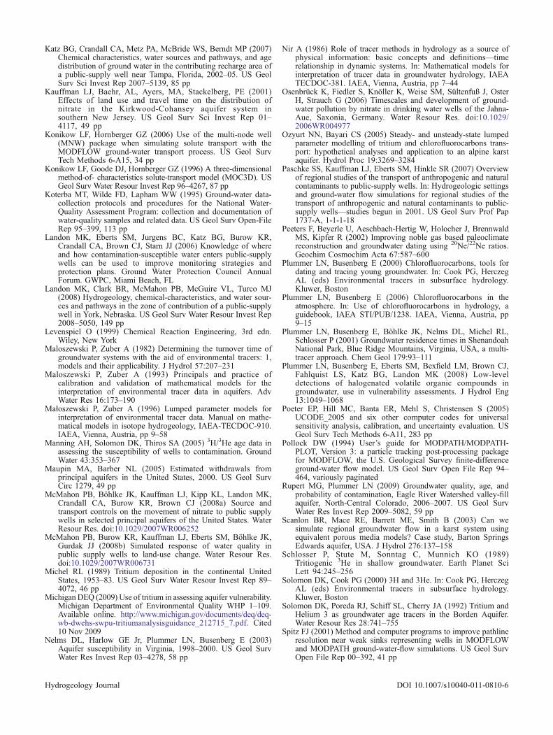
Katz BG, Crandall CA, Metz PA, McBride WS, Berndt MP (2007)Chemical characteristics, water sources and pathways, and agedistribution of ground water in the contributing recharge area ofa public-supply well near Tampa, Florida, 2002–05. US GeolSurv Sci Invest Rep 2007–5139, 85 pp

Kauffman LJ, Baehr, AL, Ayers, MA, Stackelberg, PE (2001)Effects of land use and travel time on the distribution ofnitrate in the Kirkwood-Cohansey aquifer system insouthern New Jersey. US Geol Surv Sci Invest Rep 01–4117, 49 pp

Konikow LF, Hornberger GZ (2006) Use of the multi-node well(MNW) package when simulating solute transport with theMODFLOW ground-water transport process. US Geol SurvTech Methods 6-A15, 34 pp

Konikow LF, Goode DJ, Hornberger GZ (1996) A three-dimensionalmethod-of- characteristics solute-transport model (MOC3D). USGeol Surv Water Resour Invest Rep 96–4267, 87 pp

Koterba MT, Wilde FD, Lapham WW (1995) Ground-water data-collection protocols and procedures for the National Water-Quality Assessment Program: collection and documentation ofwater-quality samples and related data. US Geol Surv Open-FileRep 95–399, 113 pp

Landon MK, Eberts SM, Jurgens BC, Katz BG, Burow KR,Crandall CA, Brown CJ, Starn JJ (2006) Knowledge of whereand how contamination-susceptible water enters public-supplywells can be used to improve monitoring strategies andprotection plans. Ground Water Protection Council AnnualForum. GWPC, Miami Beach, FL

Landon MK, Clark BR, McMahon PB, McGuire VL, Turco MJ(2008) Hydrogeology, chemical-characteristics, and water sour-ces and pathways in the zone of contribution of a public-supplywell in York, Nebraska. US Geol Surv Water Resour Invest Rep2008–5050, 149 pp

Levenspiel O (1999) Chemical Reaction Engineering, 3rd edn.Wiley, New York

Maloszewski P, Zuber A (1982) Determining the turnover time ofgroundwater systems with the aid of environmental tracers: 1,models and their applicability. J Hydrol 57:207–231

Maloszewski P, Zuber A (1993) Principals and practice ofcalibration and validation of mathematical models for theinterpretation of environmental tracer data in aquifers. AdvWater Res 16:173–190

Małoszewski P, Zuber A (1996) Lumped parameter models forinterpretation of environmental tracer data. Manual on mathe-matical models in isotope hydrogeology, IAEA-TECDOC-910.IAEA, Vienna, Austria, pp 9–58

Manning AH, Solomon DK, Thiros SA (2005) 3H/3He age data inassessing the susceptibility of wells to contamination. GroundWater 43:353–367

Maupin MA, Barber NL (2005) Estimated withdrawals fromprincipal aquifers in the United States, 2000. US Geol SurvCirc 1279, 49 pp

McMahon PB, Böhlke JK, Kauffman LJ, Kipp KL, Landon MK,Crandall CA, Burow KR, Brown CJ (2008a) Source andtransport controls on the movement of nitrate to public supplywells in selected principal aquifers of the United States. WaterResour Res. doi:10.1029/2007WR006252

McMahon PB, Burow KR, Kauffman LJ, Eberts SM, Böhlke JK,Gurdak JJ (2008b) Simulated response of water quality inpublic supply wells to land-use change. Water Resour Res.doi:10.1029/2007WR006731

Michel RL (1989) Tritium deposition in the continental UnitedStates, 1953–83. US Geol Surv Water Resour Invest Rep 89–4072, 46 pp

Michigan DEQ (2009) Use of tritium in assessing aquifer vulnerability.Michigan Department of Environmental Quality WHP 1–109.Available online. http://www.michigan.gov/documents/deq/deq-wb-dwehs-swpu-tritiumanalysisguidance_212715_7.pdf. Cited10 Nov 2009

Nelms DL, Harlow GE Jr, Plummer LN, Busenberg E (2003)Aquifer susceptibility in Virginia, 1998–2000. US Geol SurvWater Res Invest Rep 03–4278, 58 pp

Nir A (1986) Role of tracer methods in hydrology as a source ofphysical information: basic concepts and definitions—timerelationship in dynamic systems. In: Mathematical models forinterpretation of tracer data in groundwater hydrology, IAEATECDOC-381. IAEA, Vienna, Austria, pp 7–44

Osenbrück K, Fiedler S, Knöller K, Weise SM, Sültenfuß J, OsterH, Strauch G (2006) Timescales and development of ground-water pollution by nitrate in drinking water wells of the Jahna-Aue, Saxonia, Germany. Water Resour Res. doi:10.1029/2006WR004977

Ozyurt NN, Bayari CS (2005) Steady- and unsteady-state lumpedparameter modelling of tritium and chlorofluorocarbons trans-port: hypothetical analyses and application to an alpine karstaquifer. Hydrol Proc 19:3269–3284

Paschke SS, Kauffman LJ, Eberts SM, Hinkle SR (2007) Overviewof regional studies of the transport of anthropogenic and naturalcontaminants to public-supply wells. In: Hydrogeologic settingsand ground-water flow simulations for regional studies of thetransport of anthropogenic and natural contaminants to public-supply wells—studies begun in 2001. US Geol Surv Prof Pap1737-A, 1-1-1-18

Peeters F, Beyerle U, Aeschbach-Hertig W, Holocher J, BrennwaldMS, Kipfer R (2002) Improving noble gas based paleoclimatereconstruction and groundwater dating using 20Ne/22Ne ratios.Geochim Cosmochim Acta 67:587–600

Plummer LN, Busenberg E (2000) Chlorofluorocarbons, tools fordating and tracing young groundwater. In: Cook PG, HerczegAL (eds) Environmental tracers in subsurface hydrology.Kluwer, Boston

Plummer LN, Busenberg E (2006) Chlorofluorocarbons in theatmosphere. In: Use of chlorofluorocarbons in hydrology, aguidebook, IAEA STI/PUB/1238. IAEA, Vienna, Austria, pp9–15

Plummer LN, Busenberg E, Böhlke JK, Nelms DL, Michel RL,Schlosser P (2001) Groundwater residence times in ShenandoahNational Park, Blue Ridge Mountains, Virginia, USA, a multi-tracer approach. Chem Geol 179:93–111

Plummer LN, Busenberg E, Eberts SM, Bexfield LM, Brown CJ,Fahlquist LS, Katz BG, Landon MK (2008) Low-leveldetections of halogenated volatile organic compounds ingroundwater, use in vulnerability assessments. J Hydrol Eng13:1049–1068

Poeter EP, Hill MC, Banta ER, Mehl S, Christensen S (2005)UCODE_2005 and six other computer codes for universalsensitivity analysis, calibration, and uncertainty evaluation. USGeol Surv Tech Methods 6-A11, 283 pp

Pollock DW (1994) User’s guide for MODPATH/MODPATH-PLOT, Version 3: a particle tracking post-processing packagefor MODFLOW, the U.S. Geological Survey finite-differenceground-water flow model. US Geol Surv Open File Rep 94–464, variously paginated

Rupert MG, Plummer LN (2009) Groundwater quality, age, andprobability of contamination, Eagle River Watershed valley-fillaquifer, North-Central Colorado, 2006–2007. US Geol SurvWater Res Invest Rep 2009–5082, 59 pp

Scanlon BR, Mace RE, Barrett ME, Smith B (2003) Can wesimulate regional groundwater flow in a karst system usingequivalent porous media models? Case study, Barton SpringsEdwards aquifer, USA. J Hydrol 276:137–158

Schlosser P, Stute M, Sonntag C, Munnich KO (1989)Tritiogenic 3He in shallow groundwater. Earth Planet SciLett 94:245–256

Solomon DK, Cook PG (2000) 3H and 3He. In: Cook PG, HerczegAL (eds) Environmental tracers in subsurface hydrology.Kluwer, Boston

Solomon DK, Poreda RJ, Schiff SL, Cherry JA (1992) Tritium andHelium 3 as groundwater age tracers in the Borden Aquifer.Water Resour Res 28:741–755

Spitz FJ (2001) Method and computer programs to improve pathlineresolution near weak sinks representing wells in MODFLOWand MODPATH ground-water-flow simulations. US Geol SurvOpen File Rep 00–392, 41 pp


http://dx.doi.org/10.1029/2007WR006252

http://dx.doi.org/10.1029/2007WR006731

http://www.michigan.gov/documents/deq/deq-wb-dwehs-swpu-tritiumanalysisguidance_212715_7.pdf

http://www.michigan.gov/documents/deq/deq-wb-dwehs-swpu-tritiumanalysisguidance_212715_7.pdf

http://dx.doi.org/10.1029/2006WR004977

http://dx.doi.org/10.1029/2006WR004977

Starn JJ, Brown CJ (2007) Simulations of ground-water flow andresidence time near Woodbury, Connecticut. US Geol Surv SciInvest Rep 2007–5210, 45 pp

Stewart JW, Goetz CL, Mills LR (1978) Hydrogeologic factorsaffecting the availability and quality of ground water in theTemple Terrace area, Hillsborough County, Florida. US GeolSurv Water Res Invest Rep 78–4, 38 pp

Vogel JC (1967) Investigation of groundwater flow with radiocar-bon. In: Isotopes in hydrology. IAEA, Vienna, Austria, pp 355–369

Weissmann GS, Zhang Y, LaBolle EM, Fogg GE (2002) Dispersionof groundwater age in an alluvial aquifer system. Water ResourRes 38:1–8

Zinn BA, Konikow LF (2007) Potential effects of regional pumpageon groundwater age distribution. Water Resour Res. doi:10.1029/2006WR004865

Zoellmann K, Kinzelbach W, Fulda C (2001) Environmental tracertransport (3H and SF6) in the saturated and unsaturated zones andits use in nitrate pollution management. J Hydrol 240:187–205

Zuber A (1986) On the interpretation of tracer data in variable flowsystems. J Hydrol 86:45–57

Zuber A, Witczak S, Różański K, Śliwka I, Opoka M, Mochalski P,Kuc T, Karlikowska J, Kania J, Jackowicz-Korczyński M,Duliński M (2005) Groundwater dating with 3H and SF6 inrelation to mixing patterns, transport modeling and hydro-geochemistry. Hydrol Proc 19:2247–2275


http://dx.doi.org/10.1029/2006WR004865

http://dx.doi.org/10.1029/2006WR004865

comparison of particle-tracking and lumped-parameter age ... et al supply well age... ·...

Documents