comparing the roles of barotropic versus baroclinic feedbacks in the
TRANSCRIPT

Generated using version 3.0 of the official AMS LATEX template
Comparing the roles of barotropic versus baroclinic feedbacks in1
the atmosphere’s response to mechanical forcing2
Elizabeth A. Barnes ∗
Department of Atmospheric Science, Colorado State University, Fort Collins, CO
and David W. J. Thompson
Department of Atmospheric Science, Colorado State University, Fort Collins, CO
accepted 1st Aug, 2013 for the Journal of the Atmospheric Sciences
3
∗Corresponding author address: Elizabeth A. Barnes, Department of Atmospheric Science, Colorado
State University, 1371 Campus Delivery, Fort Collins, CO 80523.
E-mail: [email protected]
1
ABSTRACT4
Do barotropic or baroclinic eddy feedbacks dominate the atmospheric circulation response5
to mechanical forcing?6
We present a methodology to address this question by imposing barotropic torques over7
a range of latitudes in both an idealized general circulation model (GCM) and a barotropic8
model. The GCM includes both baroclinic and barotropic feedbacks. The barotropic model9
is run in two configurations: (1) only barotropic feedbacks are present and (2) a baroclinic-10
like feedback is added by allowing the stirring region to move with the jet. We examine the11
relationship between the latitude of the forcing and the response by systematically shifting12
the torques between the tropics and the pole. We investigate the importance of the mean13
state by varying the position of the control jet.14
Five main findings are presented: (1) Barotropic feedbacks alone are capable of producing15
the structure of the GCM response to mechanical forcing but are not capable of accounting16
for its full magnitude. (2) Baroclinic processes generally increase the magnitude of the17
response, but do not strongly influence its structure.(3) For a given forcing, the largest18
response in all model configurations occurs 5-10 degrees poleward of the forcing latitude.19
(4) The maximum response occurs when the forcing is located approximately 10 degrees20
poleward of the control jet. (5) The circulation response weakens as the mean jet is found21
at higher latitudes in all model configurations.22
1
1. Introduction23
Understanding the extratropical atmospheric response to thermal and mechanical forcing24
is central to a range of current problems in climate dynamics. Midlatitude atmosphere/ocean25
interaction is a function of the tropospheric response to variations in surface diabatic heating;26
stratosphere/troposphere coupling is a function of the tropospheric response to changes in27
the shear of the flow at the tropopause level and/or diabatic heating in the polar stratosphere;28
the circulation response to climate change likely depends in part on the tropospheric response29
to diabatic heating in the tropical troposphere and at the surface over the Arctic. In all cases,30
the mechanisms that drive the tropospheric response are not fully understood.31
The problem lies not in the balanced response of the extratropical atmosphere to external32
forcing. The geostrophically and hydrostatically balanced response to thermal and mechan-33
ical forcing is both well understood and straightforward to estimate (Haynes and Shepherd34
1989; Haynes et al. 1991). Rather, the problem lies in understanding and predicting the35
subsequent changes in the extratropical eddy fluxes of heat and momentum. For example,36
most of the forcings above lead to meridional shifts in the “eddy driven” jet. The eddy driven37
jet is collocated with large eddy fluxes of heat in the lower troposphere and convergence of38
the eddy momentum flux at the tropopause level. Thus, understanding and predicting the39
response of the jet to external forcing can be accomplished only through understanding and40
predicting the response of its attendant wave fluxes of heat and momentum.41
The wave fluxes of momentum are particularly important, as they determine the barotropic42
component of the flow, project strongly onto the annular modes and their attendant climate43
impacts, and influence the lower tropospheric baroclinicity. The response of the wave fluxes44
2
of momentum to a given forcing can arise through two sets of processes:45
1) Through changes in the characteristics for meridional wave propagation aloft, i.e., via46
barotropic processes. For example, changes in the upper tropospheric mean flow influence47
the direction of wave propagation into the stratosphere (e.g., Chen and Robinson (1992);48
Simpson et al. (2009)), the phase speed and critical latitudes for meridionally propagating49
waves (e.g., Chen and Held (2007); Chen et al. (2008)), the barotropic stage of the lifecycle50
of baroclinic waves (Wittman et al. 2007), and the geometry of the critical latitudes on the51
poleward and equatorward flanks of the jet (e.g., Chen and Zurita-Gator (2008); Barnes52
et al. (2010); Kidston and Vallis (2012)).53
2) Through changes in the growth of wave activity in the troposphere, i.e. via baroclinic54
processes. The growth of baroclinic waves is a function of the baroclinicity (e.g., Lindzen and55
Farrell 1980), and observations reveal robust linkages between variability in the baroclinicity56
of the flow and the generation of wave activity in the lower troposphere (Thompson and57
Birner 2012). The linkages between the baroclinicity and wave generation are theorized to58
play a key role in the dynamics that drive the annular modes (e.g., Robinson (2000); Lorenz59
and Hartmann (2001)) and the extratropical response to stratospheric variability (e.g., Song60
and Robinson (2004)), to extratropical sea-surface temperature anomalies (e.g., Brayshaw61
et al. (2008)), and to the thermal forcings associated with climate change (e.g., Kushner62
et al. (2001); Yin (2005); Frierson et al. (2006); Lu et al. (2008, 2010); O’Gorman (2010);63
Butler et al. (2011)).64
The goal of this study is to present a methodology to investigate the relative importance65
of barotropic and baroclinic eddy feedbacks in determining the structure and amplitude66
of the extratropical circulation response to mechanical forcing. The study is modeled on67
3
the experiments performed in Ring and Plumb (2007), in which the dynamical core of a68
general circulation model is subject to mechanical torques placed over a range of extratropical69
latitudes. Here we perform similar experiments, but apply a wider range of mechanical70
forcings to a hierarchy of numerical models with varying representations of extratropical71
wave-mean flow interactions. As such, the results provide insight into 1) the relationships72
between the forcing and response latitudes; 2) the relationships between the forcing latitude73
and climatological-mean jet position; and 3) the physical feedbacks that play a key role in74
determining the amplitude and structure of the atmospheric response to mechanical forcing.75
The experiments are described in Section 2; results are given in Sections 3-5; discussion and76
conclusions are given in Section 6.77
2. Experiments78
We conduct a series of experiments similar to those run in Ring and Plumb (2007), in79
which the extratropical atmosphere is subjected to a series of mechanical torques centered at80
a range of latitudes. In all experiments the torque is applied as a tendency in the zonal-mean81
zonal wind. It is Gaussian in latitude with an e-folding width of ∼11o (similar to that used in82
Ring and Plumb (2007)) and maximum amplitude of 1 m/s/day. For each experiment, model83
integrations are performed with forcing applied at 5 degree latitude increments between the84
subtropics and high latitudes.85
The relative importance of barotropic and baroclinic processes in determining the circu-86
lation response to the imposed mechanical torques is assessed using the following hierarchy87
of numerical experiments.88
4

1) Experiments run on the full dynamical core of a general circulation model (GCM).89
The eddy response in the GCM reflects the full suite of (dry) baroclinic and barotropic eddy90
feedbacks present in the observed atmosphere.91
2) Experiments run on a barotropic model in which the latitude of the stirring region92
(i.e., the source of wave activity) is fixed in time. By construction, the eddy response to a93
given forcing must be due solely to barotropic eddy feedbacks from wave propagation and94
dissipation. (See schematic in Fig. 1a).95
3) Experiments run on a barotropic model in which the latitude of the stirring region is96
in part determined by the strength of the zonal flow. In this case the source of wave activity97
migrates in response to changes in both the eddy-momentum fluxes (through their influence98
on the mean winds) and the direct influence of the applied torque on the mean winds. The99
total eddy response is thus influenced by both barotropic and baroclinic processes. (See100
schematic in Fig. 1b).101
In this study, we distinguish barotropic feedbacks as those simulated by a barotropic102
model with fixed stirring (constant eddy source). This definition of barotropic feedbacks103
thus includes the interaction of the background flow with the wave propagation and dis-104
sipation. We note, however, that the barotropic model also includes the influence of the105
background vorticity gradient on the pseudomomentum source, which can also modulate the106
eddy fluxes (see Barnes and Garfinkel (2012) for discussion of this feedback). Baroclinic feed-107
backs are defined as changes in the position and strength of the eddy source due to changes108
in the low-level baroclinicity. While the GCM inherently includes a suite of barotropic and109
baroclinic feedbacks which may not be easily distinguished from one another, the subset of110
barotropic model experiments that include a baroclinic-like feedback (Experiment 3) will111
5
only directly simulate the movement of the eddy source (the “baroclinic zone”) with the112
movement of the zonal flow. We note, however, that other distinctions between barotropic113
and baroclinic feedbacks are also possible. For example, baroclinic processes may modulate114
wave characteristics such as phase speed and wave number rather than just the strength and115
position of the wave generation. We will not be directly simulating these feedback in the116
barotropic model experiments.117
Details of all experiment set-ups are provided below.118
a. Experiment 1 setup: GCM119
In the GCM experiments we apply the zonal torques to the spectral dry dynamical core120
used in Held and Suarez (1994). The model parameters are identical to those in Held and121
Suarez (1994) unless otherwise mentioned. The model is integrated at T42 resolution, with122
20 evenly spaced sigma levels and a time step of 1200 seconds. The model forcing is zonally123
and hemispherically symmetric. The applied torques are identical at all model pressure124
levels.125
We shift the location of the model control jet as follows. As noted in Simpson et al.126
(2010) and Garfinkel et al. (2013), modifying the equilibrium temperature profile in the127
model can meridionally shift the eddy-driven jet without significantly changing the jet speed128
or the eddy fluxes. Following Garfinkel et al. (2013), the control tropospheric equilibrium129
temperature profile here is set by the following equation,130
Teq(p, θ) = max
[
200K, (T0 − δTnew)
(
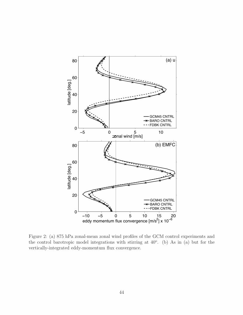
p
po
)κ]
, (1)131
6
where132
δTnew = δTHS94 + A cos(2(θ − 45o)) sin(4θ − 180o), (2)133
and the control equilibrium tropospheric temperature profile defined by Held and Suarez134
(1994) is135
δTHS94 = (∆T )y sin2(θ) + (∆T )z log(
p
p0) cos2 θ. (3)136
In all simulations, (∆T )y = 60K, (∆T )z = 10K, T0 = 315K and all other variables have137
values defined in Held and Suarez (1994).138
The GCM is run under three different control climatologies. The majority of the ex-139
periments are run in a configuration that is most like that used in Held and Suarez (1994)140
(with A = 0 in (2)), and will be referred to as GCM45 experiments since the control jet141
is located at 45o N. We will investigate the influence of jet location on the response to the142
torque in two additional experiments in which A = −2.0 (GCM43; control jet near 43o N)143
and A = +5.0 (GCM49; control jet near 49o N). Note that the TR2 and TR4 experiments144
of Simpson et al. (2010) are obtained when A = −2.0 and A = +2.0.145
The zonal-mean zonal-wind field is evaluated in the lower troposphere (875 hPa), since146
that is where friction acting on the wind field balances the vertically integrated eddy-147
momentum flux convergence. The eddy momentum flux convergence is pressure-weighted148
averaged from 1000 hPa to the top of the atmosphere, where the fluxes are first calculated149
at each pressure level before the vertical average is applied.150
Fig. 2a shows the 875 hPa zonal wind profile for the GCM45 control integration (solid151
black line). Easterlies exist near the pole and equator, and the westerlies peak near 45o - with152
this maximum defining the position of the eddy-driven jet. The near surface westerlies are153
7

maintained against drag by the eddies, and as evidenced in Fig. 2b, the vertically integrated154
eddy-momentum flux convergence (EMFC) exhibits a very similar profile to that of the low-155
level zonal-winds. The EMFC maximizes in midlatitudes and exhibits the largest divergence156
on the jet flanks where breaking Rossby waves produce an easterly torque.157
b. Experiment 2 setup: Barotropic model with no baroclinic feedback (BARO)158
The goal of the study is to identify the relative roles of barotropic and baroclinic feedbacks159
in the extratropical atmospheric response to mechanical forcing. To help identify the role160
of barotropic feedbacks, we analyze output from a stirred barotropic model on the sphere.161
In the model, stirring of the vorticity parameterizes the wave source. The distribution of162
the stirring (i.e. strength, shape and position) remains fixed at all times in the BARO163
experiments, thus ensuring that the eddy response to the applied torque is solely due to164
barotropic processes. Details of the model are given in Barnes and Garfinkel (2012) and165
Vallis et al. (2004), but we discuss key parameters and setup here.166
The barotropic model is spectral and nondivergent. Stirring is applied as an additional167
term in the vorticity tendency equation and is scale specific, with stirring over total wavenum-168
bers 8-12, requiring that the zonal wavenumber be greater than 3 in order to emphasize169
synoptic-scale eddies. The stirring is modeled as a stochastic process, with the vorticity170
tendency introduced by the stirring ranging between (-A,A) ×10−11 1/s and a decorrelation171
time of 2 days (see Vallis et al. (2004) for additional details).172
The stirring is windowed with a Gaussian in physical space (denoted W) in order to173
produce a meridionally confined storm track. The Gaussian at each time step (t) has a174
8
width given by σstir and is centered on the stirring latitude (θstir), which is set equal to a175
fixed latitude (θfixd) throughout the integration:176
W(t) = exp (−x(t)2) (4)177
x(t) =(θ − θstir(t))√
2σstir
(5)178
θstir(t) = θfixd. (6)179
In all experiments here, σstir = 12o which corresponds to a half-width of about 14o. Note180
that although the stirring shape and position do not vary with the flow, the stirring is wide181
enough to allow for meridional movement of the jet and the momentum fluxes within the182
stirring domain. The model is integrated with a time step of 1800 seconds, and each control183
run is spun up for 500 days before being integrated an additional 5000 days for analysis.184
The integrations with an imposed external torque are branched off of the control integration185
at day 500 and integrated an additional 5000 days.186
We will be comparing output from the barotropic and general circulation models to test187
the relative importance of different eddy feedbacks in the response to identical forcings.188
For this reason, we wish to limit as much as possible the differences between the model189
climatologies. To do this, we set the damping timescale, amplitude and location of the190
stirring so that two aspects of the climatology in the barotropic model match as closely as191
possible those from full GCM: 1) the latitude and strength of the maximum zonal-mean192
zonal wind and 2) the magnitude of the eddy momentum flux convergence (see Table 1).193
The crosses in Fig. 2a shows the resulting zonal-mean zonal wind for the control BARO194
experiment. The crosses in Fig. 2b show the eddy-momentum flux convergences. Here195
we have used a frictional time scale of 6.5 days, stirring strength of A = 9.0 and a fixed196
9
stirring latitude of θfixd = 40o N. The latitude and strength of the maximum zonal-mean197
zonal winds agree well with the that of the GCM by construction (Fig. 2a). However, the198
wind profiles themselves are determined purely by the eddy fluxes in each model, i.e., the199
internal dynamics of the flow. The agreement between the climatological mean zonal flow of200
the GCM and barotropic model attest to the utility of the barotropic model for simulating201
that part of the GCM zonal-wind that is driven by eddy momentum fluxes.202
c. Experiment setup 3: Barotropic model with baroclinic feedback (FDBK)203
In the BARO experiment setup described above, the stirring latitude remains fixed204
throughout the entire integration. Hence, meridional shifts in the momentum fluxes and205
zonal jet do not influence the location of the stirring. In the FDBK experiment setup, we206
use the same barotropic model and setup as in BARO, except here the latitude of the stir-207
ring is determined in part by the zonal-mean zonal flow. Specifically, a meridionally-confined208
storm track is created from the global stirring by windowing the gridded stirring field with209
a spatial mask W as in the BARO experiments. W(t) and x(t) are defined as in (4) and (5),210
but in this case:211
θstir(t) =1
2[(1− αfdbk) · θfixd + αfdbk · θjet(t)] , (7)212
where θjet(t) is the latitude of the maximum zonal-mean zonal-winds at time step t and213
is calculated during model integration at each time step. In this way, θstir moves with214
the jet to simulate the linkages between the zonal-mean upper-level flow and lower-level215
baroclinicity (i.e., since the zonal flow goes to zero at the surface, the vertical shear of the216
flow is proportional to the flow at upper levels). The location of the stirring is thus given217
10

in part by θfixd, which can be viewed as reflecting the influence on baroclinicity of forcings218
that are fixed in time (e.g., meridional gradients in radiation; ocean currents; etc), and θjet,219
which can be viewed as reflecting the influence on baroclinicity of both the momentum fluxes220
and the torque.221
The strength of the baroclinic-like feedback is set by αfdbk, which is a value between222
0 and 1. Note that when αfdbk = 0, there is no feedback between the zonal-flow and the223
latitude of the stirring regions, and the stirring is identical to that in the BARO experiment.224
The feedbacks are introduced on day 500 of the control BARO experiment to allow the jet225
and eddies to come into equilibrium without the baroclinic feedback present.226
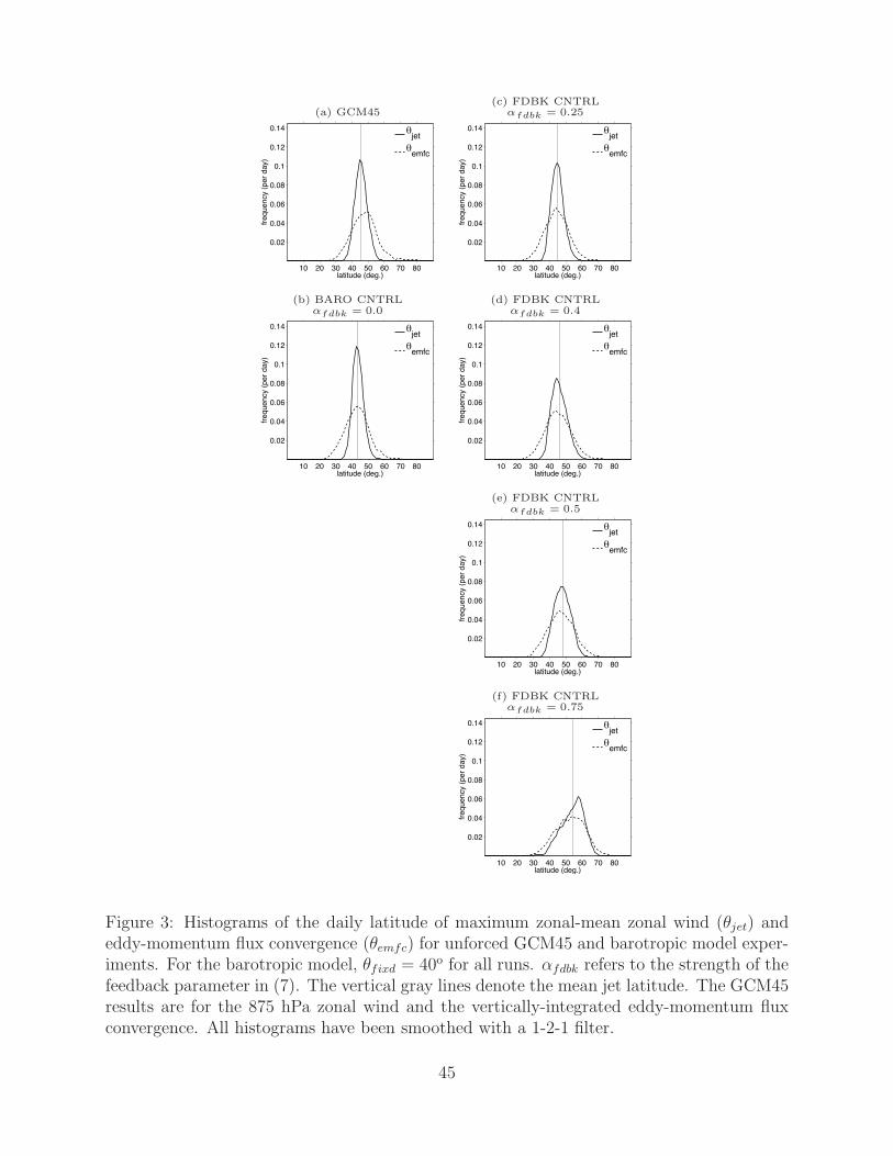
The amplitude of αfdbk was chosen as follows. Fig. 3a,b shows histograms of the daily227
latitude of θjet (solid black lines) and θemfc (the latitude of the maximum eddy-momentum228
flux convergence; dashed black lines) for the control (unforced) GCM45 and BARO runs.229
Both the GCM and the barotropic model show distributions of jet latitude that are nar-230
rower than the distributions of the eddy-momentum flux convergence, highlighting that the231
maximum eddy forcing on daily time scales does not always align with the zonal jet. This is232
possible when the zonal-wind acceleration due to the shifted eddy forcing is not enough to233
shift the zonal-wind maximum. Note, however, that the eddy-momentum flux convergence234
and the surface winds must balance in steady state.235
Careful comparison of Fig. 3a and Fig. 3b demonstrates that the widths of the distribu-236
tions of θjet and θemfc are larger in GCM45 than BARO, implying that the jet and eddies237
can move further away from their time-mean locations in the GCM. Table 2 shows that this238
is the case, where the standard deviations of θjet is 4.0o in the GCM, but 3.0o in BARO and239
the standard deviation of θemfc is 1.0o larger in the GCM.240
11

We run 5 different FDBK control experiments, where αfdbk varies between 0.25 and 0.75.241
The histograms are shown in Fig. 3c-f and the corresponding spreads are given in Table 2. As242
the feedback is increased in the barotropic model (αfdbk increases), the standard deviation243
of θjet and θemfc increases as well, demonstrating that increasing the feedback parameter244
allows the eddies and the eddy-driven jet to shift further from θfixd on any given day.245
For αfdbk = 0.25, the mean jet position (vertical lines in Fig. 3) remains near 45oN,246
similar to the BARO and GCM45 experiments. However, for αfdbk ≥ 0.4, the jet and EMFC247
distributions shift poleward. This propensity for the eddies and jet to migrate poleward is248
likely due the mechanism first explored Feldstein and Lee (1998), where the preference for249
waves to propagate and break on the equatorward flank of the jet causes the jet and eddies250
to shift poleward over time.251
For the subsequent analysis, we have chosen to set the feedback parameter αfdbk=0.4. An252
αfdbk of 0.4 gives the largest agreement between the GCM response and the barotropic model253
response (quantified by the spatial covariance of the responses to be discussed in Section 4).254
In addition, an αfdbk of 0.4 gives an e-folding timescale (τ) of the FDBK control annular255
mode time series (the annular mode is defined as the leading EOF of the zonal-mean zonal256
wind) of approximately 13 days. This value compares reasonably well with the observed257
e-folding time scale of the tropospheric Southern Annular Mode (Gerber et al. 2008). We258
note, however, that while the FDBK control experiment with αfdbk = 0.4 gives a reasonable259
annular-mode timescale, the GCM substantially overestimates this timescale by a factor260
of two (36 days). This bias in the GCM toward long-timescales is well documented and261
appears to be sensitive to model resolution, topography and mean state (Gerber and Vallis262
2007; Wang and Magnusdottir 2012). Annular mode timescales for the BARO and FDBK263
12

runs with varying feedback strengths are given in Table 3, and the persistence of the annular264
mode increases with increasing feedback strength.265
The primary results in the next section were also tested for αfdbk =0.25 and 0.5. The266
findings for these additional experiments are presented in Appendix A. The magnitude of267
the response changes as the feedback changes, but the results are otherwise qualitatively268
similar.269
3. The GCM response to an external torque270
We will first discuss the circulation response in the GCM45 experiments. By construction,271
the response includes the full suite of (dry) baroclinic and barotropic feedbacks. We will then272
compare the full GCM responses to those derived from the barotropic model experiments273
with different representations of the eddy feedbacks.274
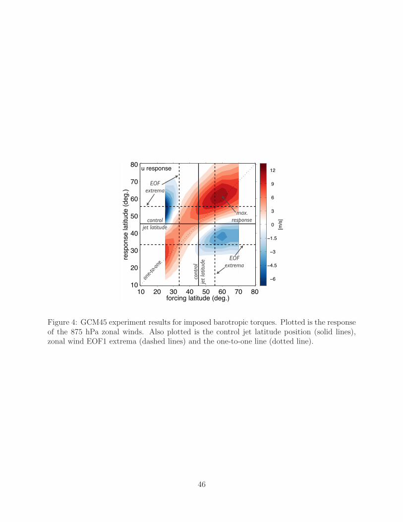
Fig. 4 shows the zonal-mean near surface zonal wind response in the GCM45 experiments.275
The format used to construct Fig. 4 will be used throughout the study. The abscissa denotes276
the latitude at which the forcing is centered; the ordinate is used to denote the latitude of277
the response; the slanted black line denotes the one-to-one line (i.e., if the response occurred278
at the same latitude as the forcing, it would lie along the one-to-one line). The thick solid279
lines denote the position of the control jet and the dashed lines denote the centers of action280
of the model annular mode in the zonal-mean zonal wind. In the GCM45 simulations, the281
control jet lies at 45.4o N and the centers of action of the annular modes at 35.4o N and282
54.5o N. The forcing is applied between 25oN to 70oN in increments of 5o. We do not apply283
the forcing equatorward of 25oN since the momentum balance in the GCM and barotropic284
13

model differ significantly there, with the GCM exhibiting a Hadley circulation which the285
barotropic model cannot simulate.286
Before we consider the responses in Fig. 4, it is useful to consider the response that would287
result in the absence of eddy feedbacks. At steady-state the vertically integrated zonal-mean288
momentum equation can be approximated as:289
0 =<∂(u
′
v′
)
∂y> −usfc
τf+ Ftorque (8)290
where Ftorque denotes the external momentum forcing, usfc the boundary layer wind, τf the291
frictional damping timescale, and <> the vertical integral. If the eddy fluxes are unchanged,292
then the torque is balanced by friction and:293
Ftorqueτf ∼ usfc. (9)294
Hence in the absence of eddy feedbacks, the zonal wind response in Fig. 4 would be organized295
along the one-to-one line with the same amplitude at all latitudes. (This can be seen in Fig.296
8a where we show that the zonal-mean zonal wind response lies along the forcing axis in the297
barotropic model with no eddies (A = 0).) Clearly, this is not the shape of the response in298
Fig. 4. Consistent with Ring and Plumb (2007), the response peaks not when the forcing is299
applied at the axis of the jet (45o), but when it is applied on the jet flank (55o). The easterly300
wind anomalies in the figure are the hallmark of the eddy forcing, as discussed below.301
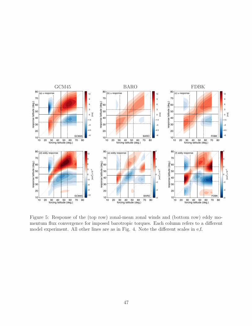
The results in Fig. 4 are reproduced in Fig. 5a. Fig. 5d shows the corresponding changes302
in the eddy momentum flux convergence. The most robust aspect of the GCM eddy response303
is that the imposed torque leads to changes in the eddy fluxes of momentum, regardless of304
the latitude of the forcing. Beyond this, the response can be divided into two regimes:305
14
(1) When the torque is applied between latitudes 25o-60o N, the eddy response is marked306
by anomalous eddy-momentum flux convergence on the poleward side of the forcing and307
anomalous eddy-momentum flux divergence on the equatorward side of the forcing. The308
eddies thus act to shift the zonal winds poleward of where they would equilibrate with309
the torque alone.310
(2) When the torque is applied poleward of 60oN, the anomalous eddy-momentum flux311
convergence maximum is located south of the torque.312
The results in Fig. 5d confirm that the eddy response to mechanical forcing is largest313
when the forcing is applied on the jet flank, but they also reveal that regardless of the forcing314
latitude, the maximum zonal wind response lies roughly 5o-10o poleward of the torque. For315
example, when the forcing coincides with the poleward center of the model annular mode316
(55o N), the response itself peaks near (65o N).317
That the eddy response lies poleward of the forcing latitude is consistent with the nature318
of meridionally propagating waves. In regions where the flow already permits a range of319
phase speeds, increases in the flow have little effect on the range of phase speeds that are320
permitted there. In contrast, in regions where the flow is relatively weak, incremental changes321
in the zonal flow have a much larger effect on the range of phase speeds permitted there.322
The changes in the wave forcing should thus peak on the flanks of the jet, where the flow is323
relatively weak, thus shifting the jet poleward (or equatorward, in the case of a low-latitude324
torque).325
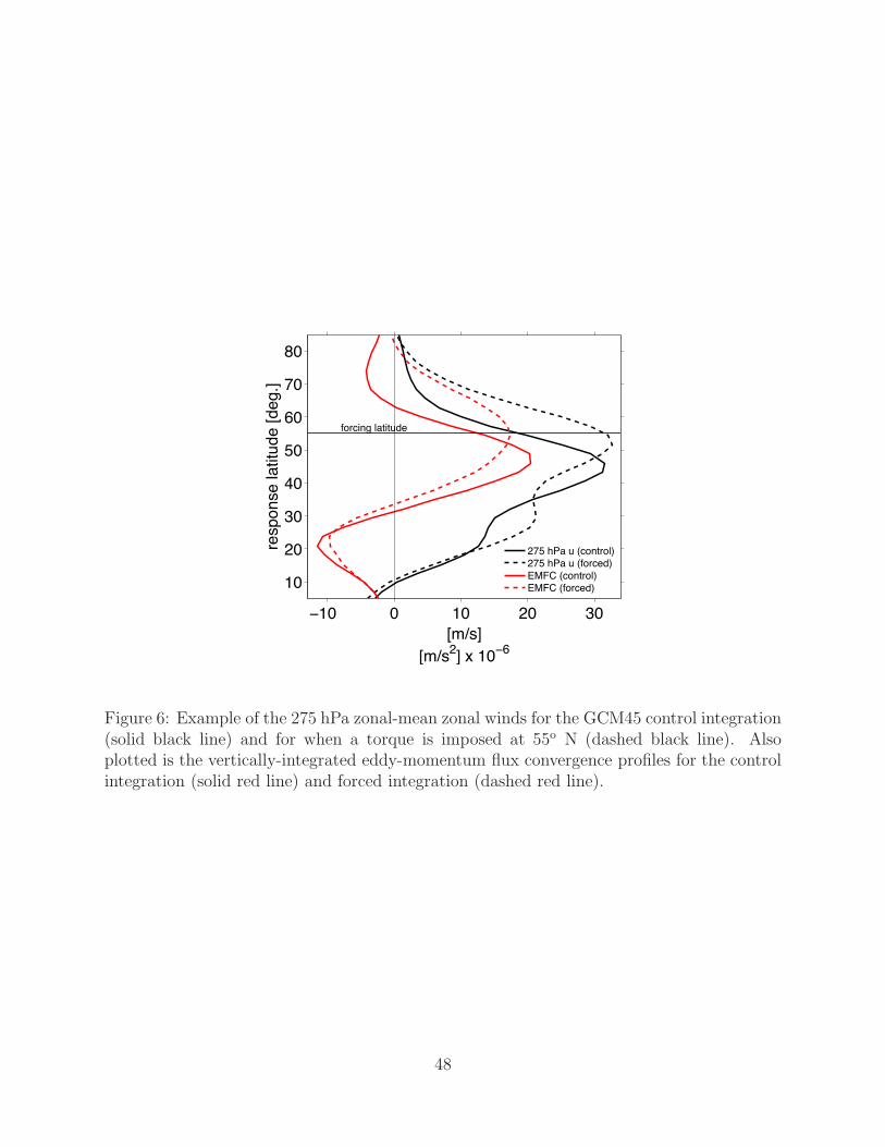
For example, consider Fig. 6, where we plot the upper-level (275 hPa) zonal-mean zonal326
winds for the GCM45 control (solid black curve) and the integration with an imposed torque327
15
at 55oN (dashed black curve). The red curves denote the total eddy-momentum flux con-328
vergence profiles for each integration. The winds increase by 14 m/s at the latitude of the329
forcing (from ∼18 to 32 m/s) and 6 m/s on the flank of the jet at 70o N (from ∼4 to 10330
m/s). The increase in wind speed is larger at the latitude of the forcing, but has a relatively331
small effect on the phase speeds permitted there since (1) waves with phase speeds <18332
m/s account for the majority of the momentum fluxes in the extratropics; and 2) waves333
with phase speeds from 0-18 m/s were already permitted at the latitude of the forcing. It334
follows that the relatively small increase in the flow from 4 to 10 m/s at 70o N has a more335
pronounced effect on the permitted wave fluxes.336
Fig. 5a,d demonstrates that the eddies induce a dipolar response in the winds for forcing337
on the flanks of the control jet. When the torque is applied at the latitude of the control338
jet, the zonal wind response is weak since the eddies oppose the torque there, i.e., there339
is anomalous divergence at the torque latitude. Similar conclusions were reached in RP07,340
but our inclusion of forcings across a wider range of latitudes yields the following additional341
insights into the GCM response to mechanical forcing:342
(1) For each forcing latitude, the maximum wind and eddy response lies 5o-10o poleward343
of the forcing. The eddies thus act to shift the zonal winds poleward of where they344
would equilibrate with the torque in the absence of eddy feedbacks.345
(2) The circulation response is largest when the torque is applied approximately 10o pole-346
ward of the control jet latitude. (Again, the maximum response is found 5o-10o pole-347
ward of the torque.)348
RP07 suggest that the maximum wind response occurs when the torque projects onto the349
16

centers of action of the annular mode in the wind field. We find a similar result for GCM 45350
but for two key additional findings: (1) consistent with (1) above, the maximum response is351
shifted poleward of the annular mode maximum and (2) as we note in Section 5, the response352
is sensitive to the climatological mean-state of the flow.353
Since part of the motivation for this work is to extend the results of RP07, Appendix B354
presents additional GCM simulations using parameters similar to those used in RP07.355
4. Barotropic vs baroclinic feedbacks356
The response of the GCM to mechanical forcing includes both (dry) barotropic and357
baroclinic eddy feedbacks. In this section we will use the BARO and FDBK configurations358
to estimate the relative importance of each feedback process in the circulation response. The359
middle and right columns of Fig. 5 show the results from the barotropic model experiments:360
the barotropic case (BARO; middle) and the case where the eddy source moves with the peak361
in the zonal-mean zonal winds (FDBK; right). The wind responses in both barotropic model362
configurations are dominated by accelerated winds along the torque axis, with the weakest363
responses found when the forcing is near the control jet latitude (as is true for the GCM).364
Both experiments also exhibit dipolar responses in the winds when the forcing is placed on365
the flanks of the jet. In all cases, the wind responses are weaker in the runs without the366
baroclinic eddy feedback.367
The eddy responses can be divided into two regimes: (1) the forcing is located south368
of ∼60o N and the barotropic eddy feedbacks act against the torque over a latitude band369
centered around the forcing and support the torque poleward of the forcing (Fig. 5e) and370
17

(2) the forcing is located poleward of ∼60o N and the eddy response is restricted to latitudes371
equatorward of the forcing. In the case of (1), the barotropic eddy feedbacks act against the372
torque for forcing near the jet latitude (blue shading near 45o N in Fig. 5e) consistent with373
the findings of Barnes and Garfinkel (2012) where they demonstrated that barotropic eddies374
oppose external forcing on the mean flow at the latitude of the forcing.375
The eddy responses in the GCM45, BARO and FDBK experiments exhibit several sim-376
ilarities. In all configurations, forcings located equatorward of ∼60o N are associated with377
eddy-momentum flux convergence poleward of the forcing and eddy momentum flux diver-378
gence equatorward of the forcing. Forcings located poleward of ∼60o N are associated with379
eddy-momentum flux convergence and divergence anomalies that are both centered equator-380
ward of the forcing. The primary difference between BARO and FDBK lies in the magnitude381
of the responses: in general the eddy response is 50% larger in the FDBK configuration. For382
the most part, it appears that barotropic dynamics may play a key role in setting the struc-383
ture of the response in the GCM, while baroclinic feedbacks set the amplitude. Note that384
both GCM45 and FDBK show local maxima in the eddy response when the forcing is placed385
near the EOF maximum and similarities between the GCM and FDBK wind responses are386
also notable in this region. On the other hand, BARO exhibits a local eddy response max-387
imum when the forcing is placed just poleward of the jet latitude, and this is not found in388
the GCM or FDBK results.389
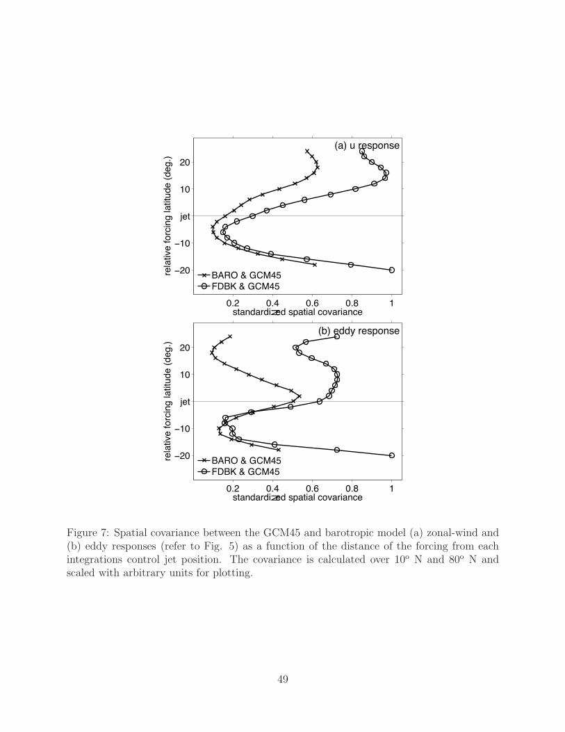
Fig. 7 quantifies the similarities and differences between (1) the GCM45 response and390
(2) the responses of the two barotropic model configurations. The figure shows the spatial391
covariance of the responses between 10o and 80o N. The response fields are first interpolated392
to a 0.5o grid, and then the response profiles for different forcing positions are projected393
18
onto each other as a function of the distance of the forcing from the control jet. This is394
done to account for differences in the mean states of the various model configurations. The395
covariance (rather than correlation) is chosen so as to take into account both the pattern396
and magnitude of the responses, and the values are scaled so that the largest agreement is397
equal to 1.398
Fig. 7a reveals that the addition of a baroclinic-like feedback to the barotropic model399
acts to noticeably improve the zonal wind response similarities with the full GCM response.400
The improvement is evident for all forcing latitudes. The agreement between the zonal wind401
responses for both BARO and FDBK and the GCM response are largest for forcing on the402
flanks of the control jet, and smallest for forcing about 5o S of the control jet.403
Fig. 7b shows the associated spatial covariances of the eddy responses (Fig. 5d-f). Again,404
for forcing on the flanks of the jet, the FDBK experiment provides better agreement with the405
GCM than the BARO experiment. And again, the agreement with the GCM is lowest just406
south of the control jet latitude for both experiments. In general, the FDBK experiment does407
a better job than BARO for forcings applied poleward of the jet and similarly for forcings408
applied equatorward. The weak agreements between the GCM and FDBK responses is409
visually apparent in Fig. 5d,f, where FDBK exhibits little response for forcing 10o south of410
the jet.411
Thus, the FDBK results suggest that a key to simulating the GCM response for forcing412
away from the jet is allowing the stirring region, and thus the baroclinic zone, to move with413
the circulation. Comparing BARO with FDBK in Fig. 5e,f, barotropic feedbacks appear to414
explain approximately 2/3 of the FDBK response, leaving the other 1/3 to be explained by415
baroclinic-like feedbacks.416
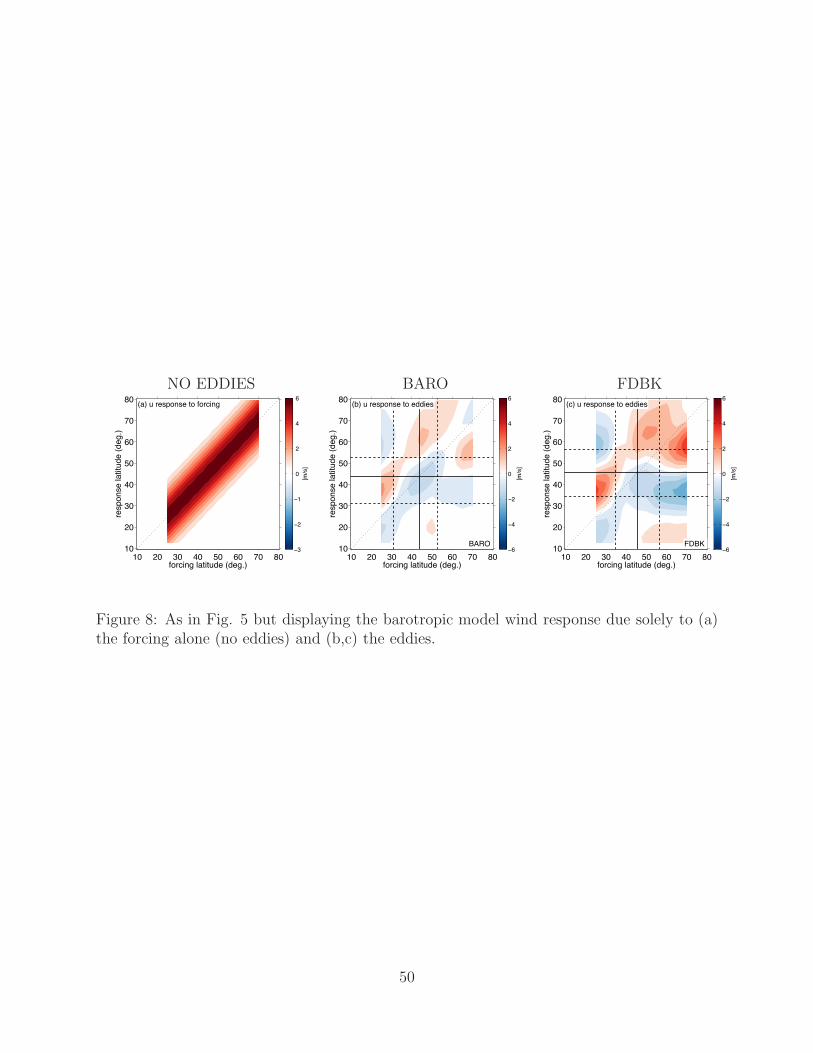
19

Finally, we quantify the magnitude of the wind response due solely to the eddies in the417
barotropic experiments. In the barotropic model, the control winds are purely eddy-driven,418
allowing the direct response of the zonal winds to the torque to be computed. As shown in419
(9) and Fig. 8a, we can empirically determine the response of the winds due purely to the420
torque by running additional barotropic model experiments without eddies (where A = 0).421
In this case,422
usfc = τfFtorque. (10)423
We have performed such integrations, and find that the maximum wind response is approx-424
imately 6.0 m/s (refer to Fig. 8a). (10) predicts a maximum of 6.5 m/s, but neglects the425
higher order diffusion term in the model that removes enstrophy at small scales, resulting in426
a slightly weaker wind response.427
By subtracting usfc (Fig. 8a) from the total zonal-mean zonal wind response of the forced428
integrations with eddies (Fig. 5b,c), one can calculate the indirect response of the winds429
to the torque via eddy feedbacks alone (Fig. 8b,c). Note that since the torque is zonally430
symmetric and thus applied only to the zonal-mean budget, the eddy response is brought431
about solely by changes in the zonal-mean winds and thus signifies either a barotropic or432
baroclinic-like eddy-mean flow feedback. As expected, eddy feedbacks explain all of the wind433
response away from the torque latitude. For forcing near the jet center, the eddies generally434
oppose the torque.435
20

5. Dependence of the response on the mean state436
In this section, we investigate the role of the mean state on the response of the circulation437
to an external torque. We perform this analysis based upon the recent results of Garfinkel438
et al. (2013) and Simpson et al. (2010, 2012), where the magnitude of the tropospheric439
jet response to stratospheric forcing decreases as the mean jet is located further from the440
equator. Consistent with those studies, Barnes and Hartmann (2011) and Barnes and Polvani441
(2013) demonstrate that the meridional shifts in the flow associated with the annular mode442
varies across a range of models as a function of the mean jet latitude, with higher-latitude443
jets experiencing smaller shifts in the flow, and vice versa. By modifying the equilibrium444
temperature gradient to move the tropospheric jet (refer to Section 2), we can investigate to445
what degree the response magnitude to the same mechanical torque is a function of the mean446
jet latitude. We will show that the latitude of the jet appears to play a role in modulating447
the response, and that this effect is present in the barotropic model runs.448
a. Varying the mean state in the GCM449
Fig. 9 displays results for the three GCM configurations outlined in Section 2, with450
the GCM45 experiment repeated for comparison. The jet latitude and jet speed for each451
run are summarized in Table 1. The vertical structure of the zonal-mean zonal winds are452
shown in the top rows of Fig. 9, with the black vertical line denoting the mean jet latitude.453
The second and third rows of Fig. 9 display the response of the 875 hPa winds and the454
vertically integrated EMFC to the applied torques (as in Fig. 5). Many of the features455
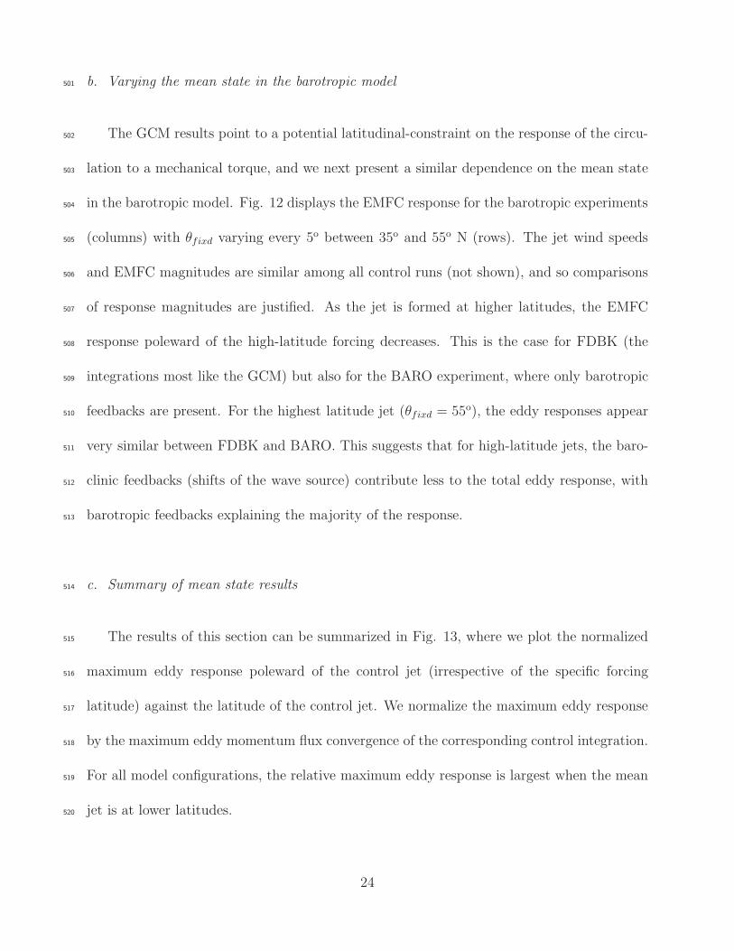
previously described for the GCM45 experiment are also present in the GCM43 and GCM49456
21
configurations and so will not be discussed here. What interests us are the differences in the457
responses between the three simulations.458
Comparison of the responses in Fig. 9 shows that contrary to the results of RP07, the459
wind and eddy responses are not always maximized for forcing at the zonal wind EOF460
latitude (dashed lines). For example, in GCM43 the maximum wind response occurs for461
forcing poleward of the zonal wind EOF maximum, near 55 N; in GCM49, the maximum eddy462
response occurs for forcing equatorward of the EOF maximum, again near 55 N. Interestingly,463
the maximum eddy response aligns remarkably well with the EOF of the eddy momentum464
flux convergence, as shown by the dashed lines in Fig. 10. With this in mind, one would465
not necessarily expect the wind response to align with the zonal wind EOF, as the wind466
response is a function of both the eddy response and the direct forcing by the torque. Hence467
the pattern of variability in the EMFC may be a better indicator of the structure of the468
circulation response to external forcing, at least on the poleward flank of the jet.469
In the rest of this section we will focus on the weakening of the wind and eddy responses to470
the torque in Fig. 9 as the jet moves poleward. A dependence on latitude of the tropospheric471
response to stratospheric perturbations was found by Garfinkel et al. (2013) and Simpson472
et al. (2010, 2012) and Fig. 9 shows a reduced wind and eddy response going from GCM43473
to GCM45 to GCM49. A weakening of the eddy response can be brought about in two474
ways (or a combination of the two): (1) a decrease in the difference between the magnitude475
of the forced and control EMFC while the structure of the EMFC remains fixed; or (2) a476
decrease in the shift of the EMFC while the magnitude of the EMFC remains fixed. We477
cannot comment on (1) since the control EMFC profiles differ by approximately 10% among478
the configurations (although the largest control EMFC corresponds to the configuration with479
22

the smallest response). We do, however, find evidence of (2), i.e., that the eddy fluxes shift480
less for higher-latitude jets. This is evident in Fig. 11a, which displays the time-mean481
EMFC profiles of the integrations where the torque is applied 10o poleward of the control482
jet latitude. The amount of shift is the distance between the peak EMFC and the zero line.483
Going from the lowest-latitude jet to the highest (blue curve, black curve, red curve), the484
amount that the eddy fluxes shift with the forcing decreases.485
The differences in eddy responses among the three GCM experiments feed back on the486
mean flow, and Fig. 11b shows that the jet shifts most when the EMFC response shifts487
most (lower latitude jets). For GCM43, the jet can shift as far as 11o from its control488
latitude, while GCM49 only shifts a maximum of 9o. These results are consistent with those489
of Garfinkel et al. (2013) and Simpson et al. (2010, 2012), where higher-latitude jets shift490
less in response to the same forcing. In addition, Table 3 confirms that the annular mode491
timescales in the GCM experiments decrease as the control jet is located at higher latitudes,492
suggestive of a weaker eddy-mean flow feedback.493
Note that unlike the model setup of Garfinkel et al. (2013) (which has a well-resolved494
stratosphere), the subtropical jet in our GCM simulations is very weak (as in Simpson et al.495
(2010)). Thus, although Garfinkel et al. (2013) and Barnes and Hartmann (2011) show that496
the circulation may also be less sensitive to a mechanical forcing for low-latitude jets in the497
presence of strong subtropical winds, our results do not directly conflict with their results498
due to the weak subtropical jet in our simulations and the fact that the midlatitude jet is499
never located south of 40o latitude in these experiments.500
23
b. Varying the mean state in the barotropic model501
The GCM results point to a potential latitudinal-constraint on the response of the circu-502
lation to a mechanical torque, and we next present a similar dependence on the mean state503
in the barotropic model. Fig. 12 displays the EMFC response for the barotropic experiments504
(columns) with θfixd varying every 5o between 35o and 55o N (rows). The jet wind speeds505
and EMFC magnitudes are similar among all control runs (not shown), and so comparisons506
of response magnitudes are justified. As the jet is formed at higher latitudes, the EMFC507
response poleward of the high-latitude forcing decreases. This is the case for FDBK (the508
integrations most like the GCM) but also for the BARO experiment, where only barotropic509
feedbacks are present. For the highest latitude jet (θfixd = 55o), the eddy responses appear510
very similar between FDBK and BARO. This suggests that for high-latitude jets, the baro-511
clinic feedbacks (shifts of the wave source) contribute less to the total eddy response, with512
barotropic feedbacks explaining the majority of the response.513
c. Summary of mean state results514
The results of this section can be summarized in Fig. 13, where we plot the normalized515
maximum eddy response poleward of the control jet (irrespective of the specific forcing516
latitude) against the latitude of the control jet. We normalize the maximum eddy response517
by the maximum eddy momentum flux convergence of the corresponding control integration.518
For all model configurations, the relative maximum eddy response is largest when the mean519
jet is at lower latitudes.520
24

6. Discussion & Conclusions521
In this study, we address the following question: “Do barotropic or baroclinic eddy feed-522
backs dominate the atmosphere’s response to a mechanical forcing?” We present a hierarchy523
of barotropic model and GCM simulations where an external torque is applied over a range524
of latitudes and the response of the circulation is analyzed. The GCM simulations include525
both barotropic and baroclinic feedbacks. The barotropic model simulations are run under526
two configurations: the first includes only barotropic feedbacks (the BARO simulations);527
the second includes both barotropic feedbacks and a parameterized baroclinic feedback (the528
FDBK simulations). Comparing the GCM, BARO and FDBK simulations allows us to esti-529
mate the relative importance of baroclinic and barotropic feedbacks in the total circulation530
response.531
The purpose of the study is thus two-fold. One, it highlights a methodology for investi-532
gating the role of different eddy feedbacks in the circulation response to mechanical torques.533
Two, it investigates the relative importance of various eddy feedbacks in the circulation534
response to mechanical forcing.535
Key findings include:536
(1) Barotropic processes are capable of capturing many aspects of the structure of the537
vertically-integrated GCM response to an external torque, but are unable to account538
for the magnitude of the response.539
(2) Baroclinic processes appear to play a key role in setting the amplitude of the atmospheric540
response. The role of baroclinic processes arises through the influence of the momentum541
fluxes and the torque on lower tropospheric baroclinicity and thus the location of the542
25

wave source.543
(3) For a given forcing, the largest response of the circulation and the eddy forcing is544
found poleward of the latitude of the applied torque, not at the latitude of the forc-545
ing. The maximum response of the circulation is found ∼5-10o poleward of the torque.546
The poleward displacement of the response is consistent with the relative effects of the547
climatological-mean and perturbed zonal flow on the range of permitted eddy phase548
speeds (Fig. 6).549
(4) The circulation response is largest when the torque is applied approximately 10o pole-550
ward of the climatological-mean jet latitude.551
(5) The magnitude of the response to a torque is a function of the mean jet latitude: the552
response to the same torque is decreased as the climatological-mean jet latitude is in-553
creased. This effect is found in the both the barotropic model and the GCM.554
These results have various implications for understanding climate variability and change.555
For examples:556
(1) Observations and numerical experiments reveal that stratospheric processes have a demon-557
strable effect on surface climate on both month-to-month timescales (Baldwin and558
Dunkerton 2001) and in association with the stratospheric ozone hole (Thompson et al.559
2011). The results shown here suggest that the structure of the tropospheric response is560
determined to first order by barotropic feedbacks at the tropopause level, and that the561
magnitude of the response is enhanced by baroclinic feedbacks (e.g., due to the influence562
of the momentum fluxes on lower tropospheric baroclinicity; Song and Robinson (2004)).563
26
(2) Climate models consistently predict a poleward shift of the jet in response to increasing564
greenhouse gases (e.g., Kushner et al. (2001); Miller et al. (2006); Barnes and Polvani565
(2013)). The methodology applied here investigates the shift of the jet in numerical566
models with varying representations of wave/mean flow interactions. The analyses thus567
provide a framework for investigating the mechanisms of the shift in more complicated568
IPCC-class climate models.569
(3) The dependence of the amplitude of the response to the mean jet latitude suggests that570
the sensitivity of the circulation to external forcing in the current climate may be an571
upper-limit on the sensitivity of the circulation in future climate states. Additionally,572
the ubiquitous equatorward jet latitude bias among climate models (Barnes and Polvani573
2013; Kidston and Gerber 2010) suggests that the current generation of climate models574
may overestimate the response of the circulation of the current climate to anthropogenic575
forcing.576
27
APPENDIX A577
Fig. 14 shows the eddy-momentum flux convergence response for αfdbk = 0.25, 0.4 and 0.5578
for the FDBK barotropic model experiment. Results are qualitatively similar in all cases579
(after one accounts for the variations in the mean jet position) demonstrating that the main580
features of the eddy response are robust to small variations in the feedback between the581
stirring position and the flow. However, stronger feedbacks give larger responses due to the582
ability of the flow to respond to the applied forcing and shift further away from θfixd.583
28
APPENDIX B584
Part of the motivation for this work is to extend the results of Ring and Plumb (2007), and585
here we briefly place their results in the context of our own. We perform an experiment586
identical to GCM45 but with the Rayleigh friction doubled to 0.5 days (from 1 day) to587
mimic the experiments performed by Ring and Plumb (2007). The only difference between588
this setup (denoted RP) and that of Ring and Plumb (2007) is that they introduce a hemi-589
spheric asymmetry in the equilibrium temperature profile in order to simulate austral winter.590
Here, we have kept the two hemispheres symmetric, but otherwise, all other parameters are591
identical to Ring and Plumb (2007) to the best of our knowledge.592
Figure Fig. 15 shows the zonal wind and eddy response for the RP experiment. The593
jet is located around 35oN, 5o south of the jet latitude in GCM43. Comparing with Fig. 9,594
the response of the eddies is larger in RP than the GCM43 case (note the different color595
scales), while the wind response is much smaller. The reduced wind response is largely596
due to the doubling of the drag in the simulation. The maximum jet shift for any forcing597
latitude in RP is 13.5o (not shown), more than the GCM experiments discussed here. The598
maximum eddy response appears relatively insensitive to the forcing latitude, unlike in the599
simulations previously discussed (and shown in Fig. 9). The reason for the flattening of the600
eddy response with respect to the forcing latitude for low-latitude jets requires additional601
study.602
Acknowledgments.603
EAB is funded by a NOAA Climate & Global Change Fellowship through the University604
Corporation of Atmospheric Research Visiting Science Program. DWJT is supported by the605
29

NSF Climate Dynamics program.606
30
607
REFERENCES608
Baldwin, M. P. and T. J. Dunkerton, 2001: Stratospheric harbingers of anomalous weather609
regimes. Science, 294 (5542), 581–584, doi:10.1126/science.1063315.610
Barnes, E. A. and C. I. Garfinkel, 2012: Barotropic impacts of surface friction on eddy kinetic611
energy and momentum fluxes: an alternative to the barotropic governor. J. Atmos. Sci.,612
69, 3028–3039, doi:10.1175/JAS-D-11-0243.1.613
Barnes, E. A. and D. L. Hartmann, 2011: Rossby-wave scales, propagation and the variability614
of eddy-driven jets. J. Atmos. Sci., 68, 2893–2908.615
Barnes, E. A., D. L. Hartmann, D. M. W. Frierson, and J. Kidston, 2010: The effect of616
latitude on the persistence of eddy-driven jets. Geophys. Res. Lett., 37, L11 804, doi:617
10.1029/2010GL043199.618
Barnes, E. A. and L. M. Polvani, 2013: Response of the midlatitude jets and of their vari-619
ability to increased greenhouse gases in the CMIP5 models. J. Climate, in press.620
Brayshaw, D. J., B. Hoskins, and M. Blackburn, 2008: The storm-track response to idealized621
SST perturbations in an aquaplanet GCM. J. Atmos. Sci., 65, 2842–2860.622
Butler, A. H., D. W. J. Thompson, and T. Birner, 2011: Isentropic slopes, downgradient623
eddy fluxes, and the extratropical atmospheric circulation response to tropical tropospheric624
heating. J. Atmos. Sci., 68, 2292–2305.625
31

Chen, G. and I. Held, 2007: Phase speed spectra and the recent poleward shift of Southern626
Hemisphere surface westerlies. Geophys. Res. Lett., 34, doi:10.1029/2007GL031200.627
Chen, G., J. Lu, and D. M. W. Frierson, 2008: Phase speed spectra and the latitude of628
surface westerlies: Interannual variability and global warming trend. J. Climate, 21, doi:629
5942-5959.630
Chen, G. and P. Zurita-Gator, 2008: The tropospheric jet response to prescribed zonal631
forcing in an idealized atmospheric model. J. Atmos. Sci., 65, doi:2254-2271.632
Chen, P. and W. A. Robinson, 1992: Propatation of planetary waves between the troposphere633
and stratosphere. J. Atmos. Sci., 49, doi:2533-2545.634
Feldstein, S. B. and S. Lee, 1998: Is the atmospheric zonal index driven by an eddy feedback?635
J. Atmos. Sci., 55, 3077–3086.636
Frierson, D. M. W., I. M. Held, and P. Zurita-Gator, 2006: A gray-radiation aquaplanet637
moist GCM: Static stability and eddy scale. J. Atmos. Sci., 63, 2548–2566.638
Garfinkel, C. I., D. W. Waugh, and E. P. Gerber, 2013: The effect of tropospheric jet latitude639
on coupling between the stratospheric polar vortex and the troposphere. J. Climate, 26,640
doi:10.1175/JCLI-D-12-00301.1.641
Gerber, E. P., L. M. Polvani, and D. Ancukiewicz, 2008: Annular mode time scales in the642
Intergovernmental Panel on Climate Change Fourth Assessment Report models. Geophys.643
Res. Lett., 35, doi:10.1029/2008GL035712.644
32

Gerber, E. P. and G. K. Vallis, 2007: Eddy-zonal flow interactions and the persistence of645
the zonal index. J. Atmos. Sci., 64, 3296–3311.646
Haynes, P. H., C. Marks, M. E. McIntyre, T. G. Shepherd, and K. P. Shine, 1991: On the647
“Downward Control” of Extratropical Diabitic Circulations by Eddy-Induced Mean Zonal648
Forces. J. Atmos. Sci., 48, 651–678.649
Haynes, P. H. and T. G. Shepherd, 1989: The importance of surface pressure changes in the650
response of the atmosphere to zonally-symmetric thermal and mechanical forcing. Quart.651
J. Roy. Meteor. Soc., 115, 1181–1208.652
Held, I. M. and M. J. Suarez, 1994: A proposal for the intercomparison of the dynamical653
cores of atmospheric general circulation models. Bull. Amer. Meteor. Soc., 75, 1825–1830.654
Kidston, J. and E. Gerber, 2010: Intermodel variability of the poleward shift of the austral655
jet stream in the CMIP3 integrations linked to biases in the 20th century climatology.656
Geophys. Res. Lett., 37, L09 708, doi:10.1029/2010GL042873.657
Kidston, J. and G. K. Vallis, 2012: The relationship between the speed and the latitude658
of an eddy-driven jet in a stirred barotropic model. J. Atmos. Sci., 69, doi:10.1175/659
JAS-D-11-0300.1.660
Kushner, P. J., I. M. Held, and T. L. Delworth, 2001: Southern Hemisphere atmospheric661
circulation response to global warming. J. Climate, 14, 2238–2249.662
Lorenz, D. J. and D. L. Hartmann, 2001: Eddy-zonal flow feedback in the Southern Hemi-663
sphere. J. Atmos. Sci., 58, 3312–3327.664
33
Lu, J., G. Chen, and D. M. Frierson, 2008: Response of the zonal mean atmospheric circu-665
lation to El Nino versus global warming. J. Climate, 21, 5835–5851.666
Lu, J., G. Chen, and D. M. Frierson, 2010: The position of the midlatitude storm track and667
eddy-driven westerlies in aquaplanet agcms. J. Atmos. Sci., 67, 3984–4000.668
Miller, R. L., G. A. Schmidt, and D. T. Shindell, 2006: Forced annular variations in the669
20th century intergovernmental panel on climate change fourth assessment report models.670
J. Geophys. Res., 111, doi:10.1029/2005JD006323.671
O’Gorman, P. A., 2010: Understanding the varied response of the extratropical storm tracks672
to climate change. Proc. Natl. Acad. Sci. (USA), 107, 19 176–19 180.673
Ring, M. J. and R. A. Plumb, 2007: Forced annular mode patterns in a simple atmospheric674
general circulation model. J. Atmos. Sci., 64, 3611–3626, doi:10.1175/JAS4031.1.675
Robinson, W. A., 2000: A baroclinic mechanism for the eddy feedback on the zonal index.676
J. Atmos. Sci., 57, 415–422.677
Simpson, I. R., M. Blackburn, and J. D. Haigh, 2009: The role of eddies in driving the678
tropospheric response to stratospheric heating perturbations. J. Atmos. Sci., 66, 1347–679
1365.680
Simpson, I. R., M. Blackburn, and J. D. Haigh, 2012: A mechanism for the effect of tropo-681
spheric jet structure on the annular mode like response to stratospheric forcing. JAS, 69,682
2152–2170.683
Simpson, I. R., M. Blackburn, J. D. Haigh, and S. N. Sparrow, 2010: The impact of the684
34
state of the troposphere on the response to stratospheric heating in a simplified GCM. J.685
Climate, 23, 6166–6185.686
Song, Y. and W. A. Robinson, 2004: Dynamical mechanisms for stratospheric influences on687
the troposphere. J. Atmos. Sci., 61, 1711–1725.688
Thompson, D. W. J. and T. Birner, 2012: On the linkages between the tropospheric isen-689
tropic slope and eddy fluxes of heat during Northern Hemisphere winter. J. Atmos. Sci.,690
69, 1811–1823, doi:10.1175/JAS-D-11-0187.1.691
Thompson, D. W. J., S. Solomon, P. J. Kushner, M. H. England, K. M. Grise, and D. J.692
Karoly, 2011: Signatures of the Antarctic ozone hole in Southern Hemisphere surface693
climate change. Nature Geoscience, 4 (11), 741–749, doi:10.1038/ngeo1296.694
Vallis, G. K., E. P. Gerber, P. J. Kushner, and B. A. Cash, 2004: A mechanism and simple695
dynamical model of the North Atlantic Oscillation and annular modes. J. Atmos. Sci.,696
61, 264–280.697
Wang, Y.-H. and G. Magnusdottir, 2012: The Shift of the Northern Node of the NAO698
and Cyclonic Rossby Wave Breaking. J. Climate, 25 (22), 7973–7982, doi:10.1175/699
JCLI-D-11-00596.1.700
Wittman, M. A., A. J. Charlton, and L. M. Polvani, 2007: The effect of lower stratospheric701
shear on baroclinic instability. J. Atmos. Sci., 64, 479–496.702
Yin, J. H., 2005: A consistent poleward shift of the storm tracks in simulations of 21st703
century climate. Geophys. Res. Lett., 32, doi:10.1029/2005GL023684.704
35
List of Tables705
1 Summary of mean states in the control simulations. The GCM values are706
calculated using the 875 hPa level winds. Values have been rounded to the707
nearest 0.2o and 0.5 m/s. 37708
2 Standard deviation of the daily latitude of the maximum zonal-mean zonal709
winds (σjet) and zonal-mean eddy-momentum flux convergence (σemfc) for un-710
forced GCM45 and barotropic model experiments. For the barotropic model711
experiments, θfixd = 40o for all runs. αfdbk refers to the strength of the feed-712
back. The GCM45 results are for the 875 hPa zonal wind and the vertically-713
integrated eddy-momentum flux convergence. Values have been rounded to714
the nearest 0.5o. 38715
3 Annular-mode e-folding timescales (τ) for the GCM and barotropic model716
integrations where θfixd = 45oN and θfdbk refers to the strength of the feedback717
parameter in (7). 39718
36
gcm cntrl baro cntrl fdbk cntrl
name ulat [o] uspd [m/s] θfixd ulat [o] uspd [m/s] θfixd ulat [o] uspd [m/s]
GCM43 42.8o 10.5 35o 38.0o 11.0 35o 39.8o 10.5
GCM45 45.4o 11.0 40o 43.6o 10.5 40o 45.8o 10.0
GCM49 49.4o 12.0 45o 49.2o 10.5 45o 52.4o 10.5
50o 54.7o 10.5 50o 57.2o 11.0
55o 59.0o 11.0 55o 60.6o 11.0
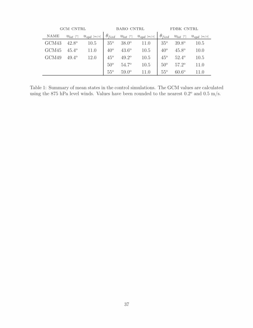
Table 1: Summary of mean states in the control simulations. The GCM values are calculatedusing the 875 hPa level winds. Values have been rounded to the nearest 0.2o and 0.5 m/s.
37
control
experiment σθjet σθemfc
gcm45 4.0o 8.5o
baro
αfdbk = 0.00 3.0o 7.5o
fdbk
αfdbk = 0.25 4.0o 7.5o
αfdbk = 0.40 4.5o 8.0o
αfdbk = 0.50 5.0o 8.5o
αfdbk = 0.75 7.0o 9.0o
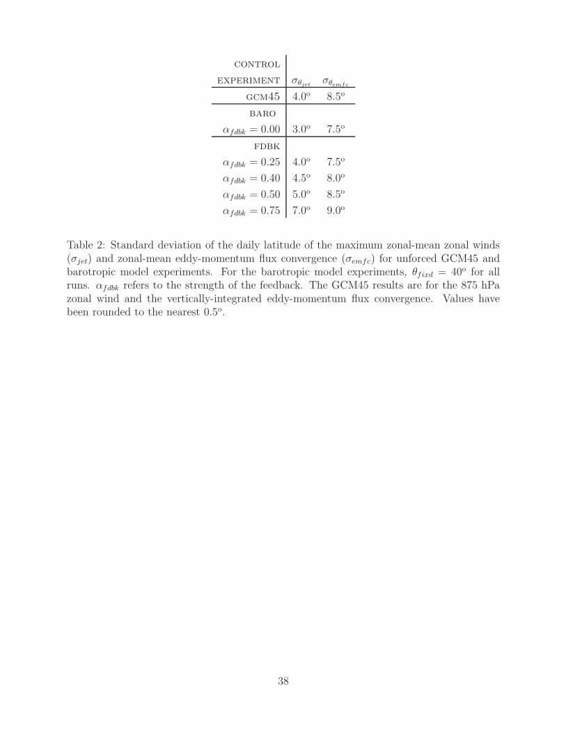
Table 2: Standard deviation of the daily latitude of the maximum zonal-mean zonal winds(σjet) and zonal-mean eddy-momentum flux convergence (σemfc) for unforced GCM45 andbarotropic model experiments. For the barotropic model experiments, θfixd = 40o for allruns. αfdbk refers to the strength of the feedback. The GCM45 results are for the 875 hPazonal wind and the vertically-integrated eddy-momentum flux convergence. Values havebeen rounded to the nearest 0.5o.
38

gcm cntrl baro & fdbk cntrl
τ [dys] αfdbk τ [dys]
GCM43 41 0.00 6
GCM45 36 0.25 9
GCM49 20 0.40 13
0.50 13
0.75 22
Table 3: Annular-mode e-folding timescales (τ) for the GCM and barotropic model inte-grations where θfixd = 45oN and θfdbk refers to the strength of the feedback parameter in(7).
39
List of Figures719
1 Schematics of the barotropic model experimental setups: (a) stirring is fixed720
for the entire run and (b) stirring latitude is partially determined by the721
latitude of maximum zonal-mean zonal winds. Gray curves denote the control722
run, and the black curves denote the runs forced with an imposed torque723
poleward of the control jet. Horizontal squiggles denote the stirring region,724
and vertical squiggles denote the eddy wave propagation away from the stirring725
region. 43726
2 (a) 875 hPa zonal-mean zonal wind profiles of the GCM control experiments727
and the control barotropic model integrations with stirring at 40o. (b) As in728
(a) but for the vertically-integrated eddy-momentum flux convergence. 44729
3 Histograms of the daily latitude of maximum zonal-mean zonal wind (θjet) and730
eddy-momentum flux convergence (θemfc) for unforced GCM45 and barotropic731
model experiments. For the barotropic model, θfixd = 40o for all runs. αfdbk732
refers to the strength of the feedback parameter in (7). The vertical gray733
lines denote the mean jet latitude. The GCM45 results are for the 875 hPa734
zonal wind and the vertically-integrated eddy-momentum flux convergence.735
All histograms have been smoothed with a 1-2-1 filter. 45736
4 GCM45 experiment results for imposed barotropic torques. Plotted is the737
response of the 875 hPa zonal winds. Also plotted is the control jet latitude738
position (solid lines), zonal wind EOF1 extrema (dashed lines) and the one-739
to-one line (dotted line). 46740
40

5 Response of the (top row) zonal-mean zonal winds and (bottom row) eddy741
momentum flux convergence for imposed barotropic torques. Each column742
refers to a different model experiment. All other lines are as in Fig. 4. Note743
the different scales in e,f. 47744
6 Example of the 275 hPa zonal-mean zonal winds for the GCM45 control inte-745
gration (solid black line) and for when a torque is imposed at 55o N (dashed746
black line). Also plotted is the vertically-integrated eddy-momentum flux747
convergence profiles for the control integration (solid red line) and forced in-748
tegration (dashed red line). 48749
7 Spatial covariance between the GCM45 and barotropic model (a) zonal-wind750
and (b) eddy responses (refer to Fig. 5) as a function of the distance of751
the forcing from each integrations control jet position. The covariance is752
calculated over 10o N and 80o N and scaled with arbitrary units for plotting. 49753
8 As in Fig. 5 but displaying the barotropic model wind response due solely to754
(a) the forcing alone (no eddies) and (b,c) the eddies. 50755
9 As in Fig. 5, but for the three GCM experiments only. The top panels show756
the vertical structure of the zonal-mean zonal winds for each model setup. 51757
10 As in the bottom panel of Fig. 9, but the dashed lines denote the eddy758
momentum flux convergence EOF1 extrema. 52759
41

11 (a) Total eddy momentum flux convergence for forced GCM runs when the760
torque is applied approximately 10o poleward of the jet. The curves are plot-761
ted as a function of relative latitude, defined as the distance from the control762
jet latitude for each GCM configuration. (b) The shift of the jet (latitude of763
maximum zonal-mean zonal winds) versus the relative forcing latitude (dis-764
tance from the control jet latitude) in the three GCM experiments. 53765
12 The eddy response from the barotropic model experiments (left) BARO and766
(right) FDBK for varying mean states. Stirring latitude (and thus jet latitude)767
increases from top to bottom, with θfixd denoted in the bottom right corner768
of each panel. 54769
13 Normalized maximum eddy momentum flux convergence response poleward770
of the control jet, irrespective of forcing latitude, versus the control jet lati-771
tude for all experiments and model setups. The maxima are normalized by772
the maximum eddy momentum flux convergence of the corresponding control773
integration. 55774
14 Comparison of eddy-momentum flux convergence response for varying feed-775
back parameters αfdbk for the FDBK barotropic model experiment. 56776
15 Same as in Fig. 9 except for a run setup similar to Ring and Plumb (2007).777
Note the different color scale for the eddy response compared to Fig. 9. 57778
42

stirring fixed
wave propagation
stirring shiftswith zonal flow
control zonal wind
forced zonal wind
(a)
(b)
forcing
wave propagation
forcing
control zonal wind
forced zonal wind
Figure 1: Schematics of the barotropic model experimental setups: (a) stirring is fixed forthe entire run and (b) stirring latitude is partially determined by the latitude of maximumzonal-mean zonal winds. Gray curves denote the control run, and the black curves denotethe runs forced with an imposed torque poleward of the control jet. Horizontal squigglesdenote the stirring region, and vertical squiggles denote the eddy wave propagation awayfrom the stirring region.
43
−5 0 5 100
20
40
60
80
zonal wind [m/s]
latitu
de [
deg.]
(a) u
GCM45 CNTRL
BARO CNTRL
FDBK CNTRL
−10 −5 0 5 10 15 200
20
40
60
80
eddy momentum flux convergence [m/s2] x 10
−6
latitu
de [
deg.]
(b) EMFC
GCM45 CNTRL
BARO CNTRL
FDBK CNTRL
Figure 2: (a) 875 hPa zonal-mean zonal wind profiles of the GCM control experiments andthe control barotropic model integrations with stirring at 40o. (b) As in (a) but for thevertically-integrated eddy-momentum flux convergence.
44
(c) FDBK CNTRL(a) GCM45 αfdbk = 0.25
10 20 30 40 50 60 70 80
0.02
0.04
0.06
0.08
0.1
0.12
0.14
latitude (deg.)
frequency (
per
day)
θjet
θemfc
10 20 30 40 50 60 70 80
0.02
0.04
0.06
0.08
0.1
0.12
0.14
latitude (deg.)
frequency (
per
day)
θjet
θemfc
(b) BARO CNTRL (d) FDBK CNTRLαfdbk = 0.0 αfdbk = 0.4
10 20 30 40 50 60 70 80
0.02
0.04
0.06
0.08
0.1
0.12
0.14
latitude (deg.)
frequency (
per
day)
θjet
θemfc
10 20 30 40 50 60 70 80
0.02
0.04
0.06
0.08
0.1
0.12
0.14
latitude (deg.)
frequency (
per
day)
θjet
θemfc
(e) FDBK CNTRLαfdbk = 0.5
10 20 30 40 50 60 70 80
0.02
0.04
0.06
0.08
0.1
0.12
0.14
latitude (deg.)
frequency (
per
day)
θjet
θemfc
(f) FDBK CNTRLαfdbk = 0.75
10 20 30 40 50 60 70 80
0.02
0.04
0.06
0.08
0.1
0.12
0.14
latitude (deg.)
frequency (
per
day)
θjet
θemfc
Figure 3: Histograms of the daily latitude of maximum zonal-mean zonal wind (θjet) andeddy-momentum flux convergence (θemfc) for unforced GCM45 and barotropic model exper-iments. For the barotropic model, θfixd = 40o for all runs. αfdbk refers to the strength of thefeedback parameter in (7). The vertical gray lines denote the mean jet latitude. The GCM45results are for the 875 hPa zonal wind and the vertically-integrated eddy-momentum fluxconvergence. All histograms have been smoothed with a 1-2-1 filter.
45
!" #" $" %" &" '" (" )"!"
#"
$"
%"
&"
'"
("
)"
*+,-./01234.4567186709:
,7;<+/;71234.4567186709:
1
1
51,7;<+/;7
=>?1@ABCD;E
11!'
!%9&
11!$
!!9&
111"
111$
111'
111F
11!#
EOF extrema
EOF extrema
controljet latitude
cont
rol
jet
latit
ude
one-to-one
max. response
Figure 4: GCM45 experiment results for imposed barotropic torques. Plotted is the responseof the 875 hPa zonal winds. Also plotted is the control jet latitude position (solid lines),zonal wind EOF1 extrema (dashed lines) and the one-to-one line (dotted line).
46
GCM45 BARO FDBK
10 20 30 40 50 60 70 8010
20
30
40
50
60
70
80
forcing latitude (deg.)
response latitu
de (
deg.)
u response
GCM45
(a) u response[m
/s]
−6
−4.5
−3
−1.5
0
3
6
9
12
10 20 30 40 50 60 70 8010
20
30
40
50
60
70
80
forcing latitude (deg.)
response latitu
de (
deg.)
BARO
(b) u response
[m/s
]
−6
−4.5
−3
−1.5
0
3
6
9
12
10 20 30 40 50 60 70 8010
20
30
40
50
60
70
80
forcing latitude (deg.)
response latitu
de (
deg.)
FDBK
(c) u response
[m/s
]
−6
−4.5
−3
−1.5
0
3
6
9
12
10 20 30 40 50 60 70 8010
20
30
40
50
60
70
80
forcing latitude (deg.)
response latitu
de (
deg.)
(d) eddy response
GCM45
[m/s
2]
x 1
0−
6
−12
−9
−6
−3
0
3
6
9
12
10 20 30 40 50 60 70 8010
20
30
40
50
60
70
80
forcing latitude (deg.)
response latitu
de (
deg.)
eddy response
BARO BARO
(e) eddy response
[m/s
2]
x 1
0−
6
−6
−4
−2
0
2
4
6
10 20 30 40 50 60 70 8010
20
30
40
50
60
70
80
forcing latitude (deg.)
response latitu
de (
deg.)
eddy response
FDBK FDBK
(f) eddy response
[m/s
2]
x 1
0−
6
−6
−4
−2
0
2
4
6
Figure 5: Response of the (top row) zonal-mean zonal winds and (bottom row) eddy mo-mentum flux convergence for imposed barotropic torques. Each column refers to a differentmodel experiment. All other lines are as in Fig. 4. Note the different scales in e,f.
47
−10 0 10 20 30
10
20
30
40
50
60
70
80
[m/s]
[m/s2] x 10
−6
response latitu
de [
deg.]
forcing latitude
275 hPa u (control)
275 hPa u (forced)
EMFC (control)
EMFC (forced)
Figure 6: Example of the 275 hPa zonal-mean zonal winds for the GCM45 control integration(solid black line) and for when a torque is imposed at 55o N (dashed black line). Alsoplotted is the vertically-integrated eddy-momentum flux convergence profiles for the controlintegration (solid red line) and forced integration (dashed red line).
48
0.2 0.4 0.6 0.8 1
−20
−10
jet
10
20
standardized spatial covariance
rela
tive f
orc
ing latitu
de (
deg.)
(a) u response
BARO & GCM45FDBK & GCM45
0.2 0.4 0.6 0.8 1
−20
−10
jet
10
20
standardized spatial covariance
rela
tive f
orc
ing latitu
de (
deg.)
(b) eddy response
BARO & GCM45FDBK & GCM45
Figure 7: Spatial covariance between the GCM45 and barotropic model (a) zonal-wind and(b) eddy responses (refer to Fig. 5) as a function of the distance of the forcing from eachintegrations control jet position. The covariance is calculated over 10o N and 80o N andscaled with arbitrary units for plotting.
49
NO EDDIES BARO FDBK
10 20 30 40 50 60 70 8010
20
30
40
50
60
70
80
forcing latitude (deg.)
response latitu
de (
deg.)
(a) u response to forcing
[m/s
]
−3
−2
−1
0
2
4
6
10 20 30 40 50 60 70 8010
20
30
40
50
60
70
80
forcing latitude (deg.)
response latitu
de (
deg.)
BARO
(b) u response to eddies
[m/s
]
−6
−4
−2
0
2
4
6
10 20 30 40 50 60 70 8010
20
30
40
50
60
70
80
forcing latitude (deg.)
response latitu
de (
deg.)
FDBK
(c) u response to eddies
[m/s
]
−6
−4
−2
0
2
4
6
Figure 8: As in Fig. 5 but displaying the barotropic model wind response due solely to (a)the forcing alone (no eddies) and (b,c) the eddies.
50

GCM43 GCM45 GCM49
10 20 30 40 50 60 70 80
0
200
400
600
800
latitude (deg. N)
pre
ssure
(hP
a)
GCM43
zonal w
ind (
m/s
)
−40
−30
−20
−10
0
10
20
30
40
10 20 30 40 50 60 70 80
0
200
400
600
800
latitude (deg. N)
pre
ssure
(hP
a)
GCM45
zonal w
ind (
m/s
)
−40
−30
−20
−10
0
10
20
30
40
10 20 30 40 50 60 70 80
0
200
400
600
800
latitude (deg. N)
pre
ssure
(hP
a)
GCM49
zonal w
ind (
m/s
)
−40
−30
−20
−10
0
10
20
30
40
10 20 30 40 50 60 70 8010
20
30
40
50
60
70
80
forcing latitude (deg.)
response latitu
de (
deg.)
u response
GCM43
[m/s
]
−6
−4.5
−3
−1.5
0
3
6
9
12
10 20 30 40 50 60 70 8010
20
30
40
50
60
70
80
forcing latitude (deg.)
response latitu
de (
deg.)
u response
GCM45
[m/s
]
−6
−4.5
−3
−1.5
0
3
6
9
12
10 20 30 40 50 60 70 8010
20
30
40
50
60
70
80
forcing latitude (deg.)
response latitu
de (
deg.)
u response
GCM49
[m/s
]
−6
−4.5
−3
−1.5
0
3
6
9
12
10 20 30 40 50 60 70 8010
20
30
40
50
60
70
80
forcing latitude (deg.)
response latitu
de (
deg.)
eddy response
GCM43
[m/s
2]
x 1
0−
6
−21
−18
−15
−12
−9
−6
−3
0
3
6
9
12
15
18
21
10 20 30 40 50 60 70 8010
20
30
40
50
60
70
80
forcing latitude (deg.)
response latitu
de (
deg.)
eddy response
GCM45
[m/s
2]
x 1
0−
6
−21
−18
−15
−12
−9
−6
−3
0
3
6
9
12
15
18
21
10 20 30 40 50 60 70 8010
20
30
40
50
60
70
80
forcing latitude (deg.)
response latitu
de (
deg.)
eddy response
GCM49[m
/s2]
x 1
0−
6
−21
−18
−15
−12
−9
−6
−3
0
3
6
9
12
15
18
21
Figure 9: As in Fig. 5, but for the three GCM experiments only. The top panels show thevertical structure of the zonal-mean zonal winds for each model setup.
51

GCM43 GCM45 GCM49
10 20 30 40 50 60 70 8010
20
30
40
50
60
70
80
forcing latitude (deg.)
response latitu
de (
deg.)
eddy response
GCM43
[m/s
2]
x 1
0−
6
−16
−12
−8
−4
0
4
8
12
16
10 20 30 40 50 60 70 8010
20
30
40
50
60
70
80
forcing latitude (deg.)
response latitu
de (
deg.)
eddy response
GCM45
[m/s
2]
x 1
0−
6
−16
−12
−8
−4
0
4
8
12
16
10 20 30 40 50 60 70 8010
20
30
40
50
60
70
80
forcing latitude (deg.)
response latitu
de (
deg.)
eddy response
GCM49
[m/s
2]
x 1
0−
6
−16
−12
−8
−4
0
4
8
12
16
Figure 10: As in the bottom panel of Fig. 9, but the dashed lines denote the eddy momentumflux convergence EOF1 extrema.
52
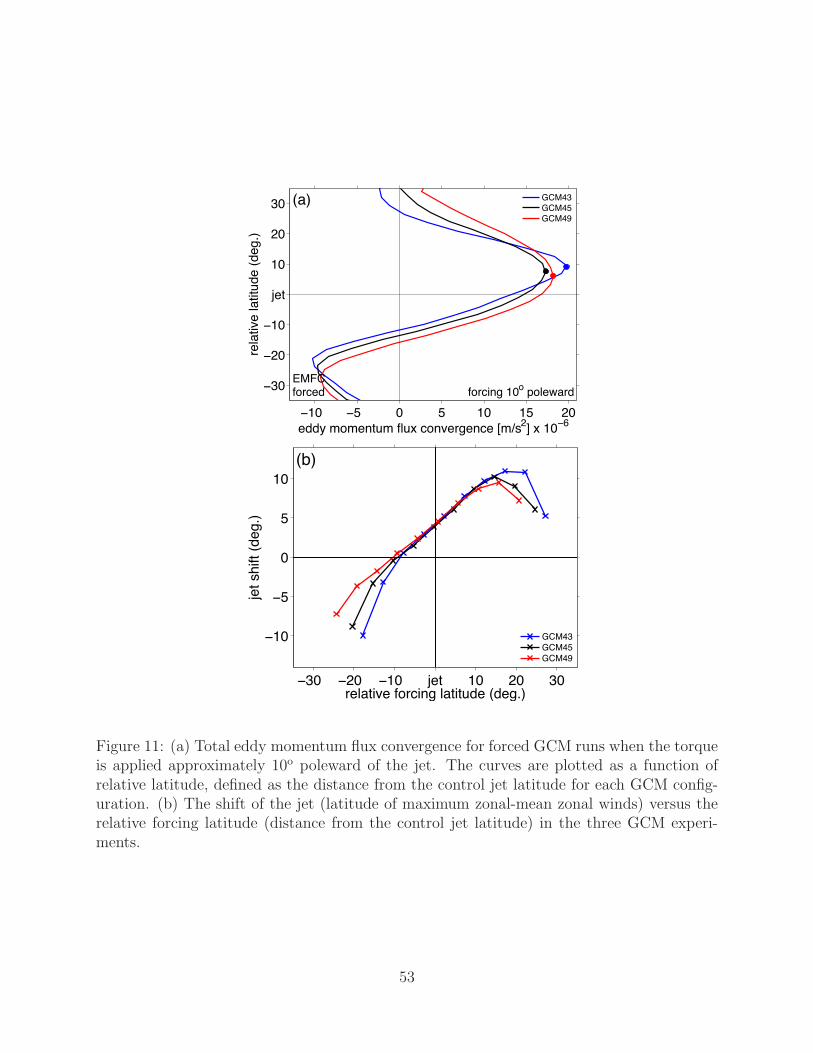
−10 −5 0 5 10 15 20
−30
−20
−10
jet
10
20
30
eddy momentum flux convergence [m/s2] x 10
−6
rela
tive latitu
de (
deg.)
EMFCforced forcing 10
o poleward
(a) GCM43
GCM45
GCM49
−30 −20 −10 jet 10 20 30
−10
−5
0
5
10
relative forcing latitude (deg.)
jet
shift
(deg.)
(b)
GCM43
GCM45
GCM49
Figure 11: (a) Total eddy momentum flux convergence for forced GCM runs when the torqueis applied approximately 10o poleward of the jet. The curves are plotted as a function ofrelative latitude, defined as the distance from the control jet latitude for each GCM config-uration. (b) The shift of the jet (latitude of maximum zonal-mean zonal winds) versus therelative forcing latitude (distance from the control jet latitude) in the three GCM experi-ments.
53

BARO FDBK
10 20 30 40 50 60 70 8010
20
30
40
50
60
70
80
forcing latitude (deg.)
response latitu
de (
deg.)
eddy response
BARO 35
[m/s
2]
x 1
0−
6
−6
−4
−2
0
2
4
6
10 20 30 40 50 60 70 8010
20
30
40
50
60
70
80
forcing latitude (deg.)
response latitu
de (
deg.)
eddy response
FDBK 35
[m/s
2]
x 1
0−
6
−6
−4
−2
0
2
4
6
10 20 30 40 50 60 70 8010
20
30
40
50
60
70
80
forcing latitude (deg.)
response latitu
de (
deg.)
eddy response
BARO
[m/s
2]
x 1
0−
6
−6
−4
−2
0
2
4
6
10 20 30 40 50 60 70 8010
20
30
40
50
60
70
80
forcing latitude (deg.)
response latitu
de (
deg.)
eddy response
FDBK
[m/s
2]
x 1
0−
6
−6
−4
−2
0
2
4
6
10 20 30 40 50 60 70 8010
20
30
40
50
60
70
80
forcing latitude (deg.)
response latitu
de (
deg.)
eddy response
BARO 45
[m/s
2]
x 1
0−
6
−6
−4
−2
0
2
4
6
10 20 30 40 50 60 70 8010
20
30
40
50
60
70
80
forcing latitude (deg.)
response latitu
de (
deg.)
eddy response
FDBK 45
[m/s
2]
x 1
0−
6
−6
−4
−2
0
2
4
6
10 20 30 40 50 60 70 8010
20
30
40
50
60
70
80
forcing latitude (deg.)
response latitu
de (
deg.)
eddy response
BARO 50
[m/s
2]
x 1
0−
6
−6
−4
−2
0
2
4
6
10 20 30 40 50 60 70 8010
20
30
40
50
60
70
80
forcing latitude (deg.)
response latitu
de (
deg.)
eddy response
FDBK 50
[m/s
2]
x 1
0−
6
−6
−4
−2
0
2
4
6
10 20 30 40 50 60 70 8010
20
30
40
50
60
70
80
forcing latitude (deg.)
response latitu
de (
deg.)
eddy response
BARO 55
[m/s
2]
x 1
0−
6
−6
−4
−2
0
2
4
6
10 20 30 40 50 60 70 8010
20
30
40
50
60
70
80
forcing latitude (deg.)
response latitu
de (
deg.)
eddy response
FDBK 55
[m/s
2]
x 1
0−
6
−6
−4
−2
0
2
4
6
Figure 12: The eddy response from the barotropic model experiments (left) BARO and(right) FDBK for varying mean states. Stirring latitude (and thus jet latitude) increasesfrom top to bottom, with θfixd denoted in the bottom right corner of each panel.
54

40 45 50 55 600
0.2
0.4
0.6
0.8
control jet latitude
norm
aliz
ed m
ax.
eddy r
esponse
GCM
BARO
FDBK
Figure 13: Normalized maximum eddy momentum flux convergence response poleward of thecontrol jet, irrespective of forcing latitude, versus the control jet latitude for all experimentsand model setups. The maxima are normalized by the maximum eddy momentum fluxconvergence of the corresponding control integration.
55

FDBK FDBK FDBK
αfdbk = 0.25 αfdbk = 0.4 αfdbk = 0.5
10 20 30 40 50 60 70 8010
20
30
40
50
60
70
80
forcing latitude (deg.)
response latitu
de (
deg.)
eddy response
FDBK
[m/s
2]
x 1
0−
6
−6
−4
−2
0
2
4
6
10 20 30 40 50 60 70 8010
20
30
40
50
60
70
80
forcing latitude (deg.)
response latitu
de (
deg.)
eddy response
FDBK
[m/s
2]
x 1
0−
6
−6
−4
−2
0
2
4
6
10 20 30 40 50 60 70 8010
20
30
40
50
60
70
80
forcing latitude (deg.)
response latitu
de (
deg.)
eddy response
FDBK
[m/s
2]
x 1
0−
6
−6
−4
−2
0
2
4
6
Figure 14: Comparison of eddy-momentum flux convergence response for varying feedbackparameters αfdbk for the FDBK barotropic model experiment.
56
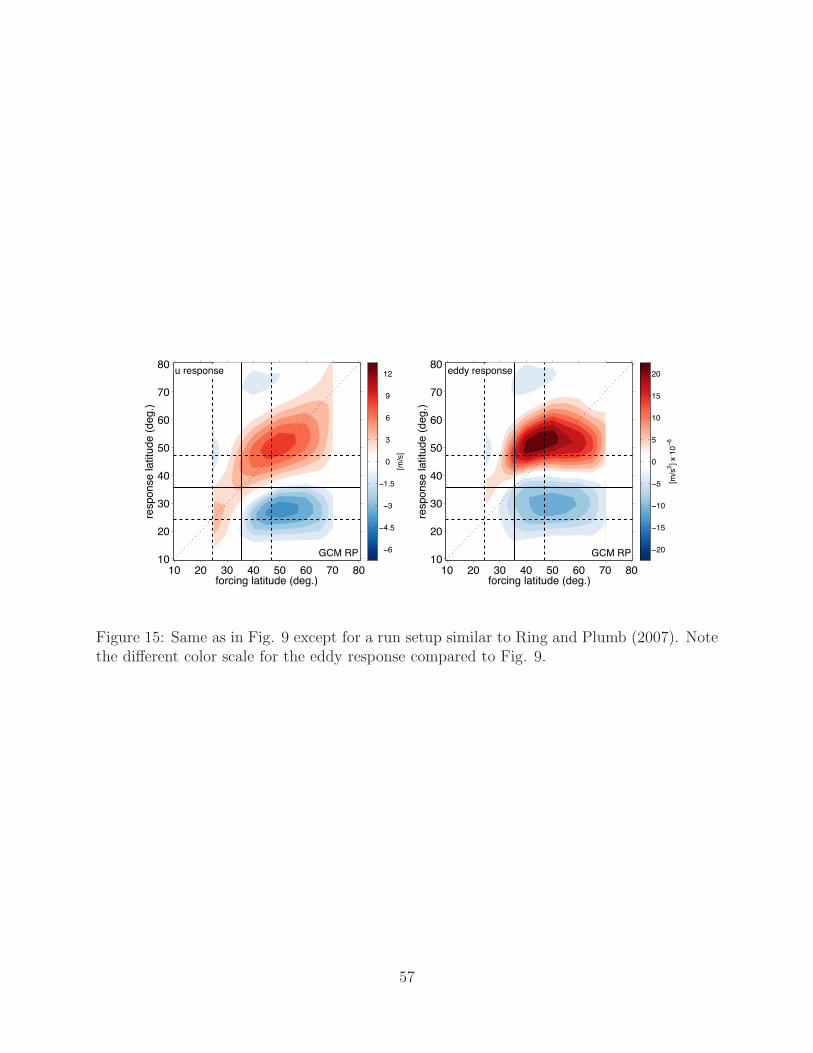
10 20 30 40 50 60 70 8010
20
30
40
50
60
70
80
forcing latitude (deg.)
response latitu
de (
deg.)
u response
GCM RP
[m/s
]
−6
−4.5
−3
−1.5
0
3
6
9
12
10 20 30 40 50 60 70 8010
20
30
40
50
60
70
80
forcing latitude (deg.)
response latitu
de (
deg.)
eddy response
GCM RP
[m/s
2]
x 1
0−
6
−20
−15
−10
−5
0
5
10
15
20
Figure 15: Same as in Fig. 9 except for a run setup similar to Ring and Plumb (2007). Notethe different color scale for the eddy response compared to Fig. 9.
57