compare sudaan & sas for brfss modeling analyses€¦ · compare sudaan & sas for brfss...

1

Compare SUDAAN & SAS for

BRFSS Modeling Analyses

Instructor: Donna Brogan, Ph.D.

March 23, 2013 Saturday PM

2013 BRFSS Annual Conference

[email protected]

2

WORKSHOP OBJECTIVES

COMPARE SURVEY PROCS

• SUDAAN • LOGISTIC (RLOGIST in SAS Callable)

• REGRESS

• SAS • SURVEYLOGISTIC

• SURVEYREG

• Interaction terms

• Predicted marginals & risk ratios

3

ASSUMED PREREQUISITES

• BRFSS survey data analysis

• SUDAAN and/or SAS survey procs

• BRFSS survey design & sampling plan

• Concepts/basics of probability sampling

• Statistical methods, using SAS STAT for SRS

• Epidemiological methods

• Linear regression & logistic regression

4

BRFSS SURVEY DESIGN

VARIABLES

Describe BRFSS RDD Sampling

Plan to SUDAAN and SAS

BRFSS Survey Design

Variables Through 2010

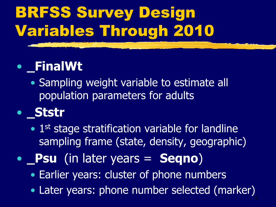
• _FinalWt

• Sampling weight variable to estimate all population parameters for adults

• _Ststr

• 1st stage stratification variable for landline sampling frame (state, density, geographic)

• _Psu (in later years = Seqno)

• Earlier years: cluster of phone numbers

• Later years: phone number selected (marker)

5

More BRFSS Survey Design

Variables Thru 2010

• Module for Sample Child

• _ChildWt, _Ststr, _Psu

• Target Popn: children reside in state in HU

• Unit of analysis = child

• Interview items about housing unit

• _HouseWt, _Ststr, _Psu

• Target Popn: HUs in state (occupied?)

• Unit of analysis = HU

6

7

BRFSS Sampling Weight

Variables through 2010

• Sum of _FinalWt over r responding adults = # adults (noninst, HH) in state popn

• Sum of _HouseWt over r responding adults = # HUs in state (occupied??)

• Sum of _ChildWt over responding adults with child data = # children (noninst, HH) in state popn

8

SAS SURVEY PROCS

Describe BRFSS RDD—1 Year

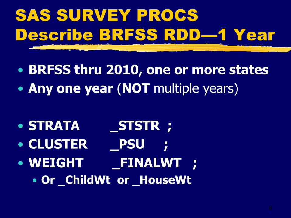
• BRFSS thru 2010, one or more states

• Any one year (NOT multiple years)

• STRATA _STSTR ;

• CLUSTER _PSU ;

• WEIGHT _FINALWT ;

• Or _ChildWt or _HouseWt

9

SUDAAN SURVEY PROCS


• BRFSS thru 2010, one or more states


• PROC ….. DESIGN = WR … ;

• NEST _STSTR _PSU ;

• WEIGHT _FINALWT ;

• Or _ChildWt or _HouseWt

Survey Design Variables:

BRFSS Dual Frame 2011 +

• _LLCPWT adult final weight

• Sampling weight variable to estimate all population parameters for adults

• _Ststr

• 1st stage stratification variable for dual frame (state, density, geographic, landline/cell)

• _Psu ( = Seqno)

• Marker for phone number selected

10

More Survey Design Vars:

BRFSS Dual Frame 2011 +

• _CLLCPWT child final weight

• Sampling weight variable to estimate all population parameters for children

• Use above with _Ststr and _Psu

• Did not find HU sampling weight variable in 2011 dual frame BRFSS dataset

• Problematic to calculate with cell phones added to 1st stage sampling frame

11

12

BRFSS Sampling Weight

Variables: 2011 onward

• Sum of _LLCPWT over r responding adults = # adults (noninst, HH) in state popn

• Sum of _CLLCPWT over responding adults with child data = # children (noninst, HH) in state popn

13

SAS SURVEY PROCS


• BRFSS 2011 +, one or more states


• STRATA _STSTR ;

• CLUSTER _PSU ;

• WEIGHT _LLCPWT ;

• Or _CLLCPWT

14

SUDAAN SURVEY PROCS


• BRFSS 0211 +, one or more states


• PROC ….. DESIGN = WR … ;

• NEST _STSTR _PSU ;

• WEIGHT _LLCPWT ;

• Or _CLLCPWT

15

BRFSS Dataset for

Workshop

LA 2004

16

BRFSS SAS Dataset

LA 2004

• n=9064 obsns (Rs)

• Geographic stratification: 9 regions (HDs?)

• Phone density stratification: listed, unlisted

• Thus, 18 strata

• Read in dataset. Go to folder BRFSData and run procformat2013.sas

17

LecEx01

_RFBING2 and _BMIR

• _RFBING2 binge drinking • 7920 no, 965 yes

• 179 missing (coded . [dot] by DB )

• _BMIR body mass index • 497 missing (coded . [dot] by DB)

• Minimum = 6.68, 8.80, 11.90

• Maximum = 99.98 (4 values), 88.38

• Nonmissing values assumed real by DB for purpose of this workshop

18

Item Nonresponse in SAS

Survey Procs: How Handled

• SAS default: MCAR

• MCAR = missing completely at random

• Assume item nonrespondents like respondents

• SAS deletes obsns with missing data from input dataset

• SAS option: NOMCAR on Proc statement

• Analyzes those who respond as subpopulation

• Those not respond used in variance estimation

19

Compare Two SAS Options

MCAR and NOMCAR

• Identical point estimates of popn parameter

• Estimated variance (s.e.) may differ slightly

• NOMCAR generally slightly higher

• Survey ddf may differ slightly

• Inference populations differ

• MCAR: target popn, e.g. all adults

• NOMCAR: subpopulation of elements who would respond to item, if asked

20

How SUDAAN Handles Item

Nonresponse in Analysis

• SUDAAN default: subpopulation analysis

• Like SAS option NOMCAR

• SUDAAN defines subpopn as those who would respond to item, if asked

• SUDAAN does subpopulation analysis, uses all obsns in dataset to estimate variances

• SAS survey procs initially had default MCAR only, then added NOMCAR option after complaints

21

DB Approach to Item

Nonresponse

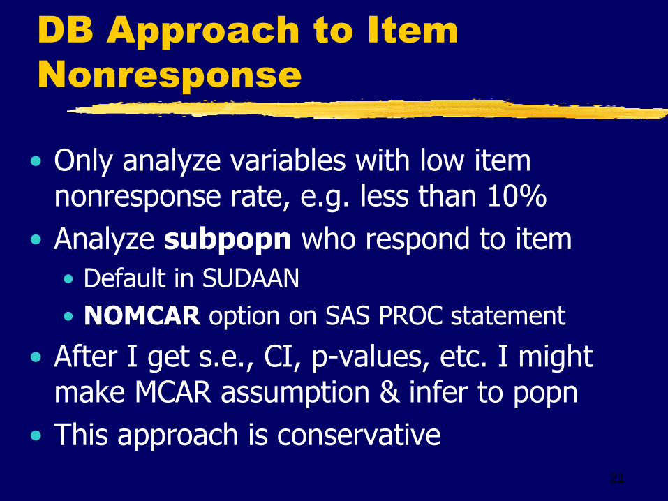
• Only analyze variables with low item nonresponse rate, e.g. less than 10%

• Analyze subpopn who respond to item

• Default in SUDAAN

• NOMCAR option on SAS PROC statement

• After I get s.e., CI, p-values, etc. I might make MCAR assumption & infer to popn

• This approach is conservative

Other Aspects of Survey

Analysis: Assume Familiar

• BRFSS variance estimation: TSL

• Taylor Series Linearization

• Default in both SUDAAN & SAS survey PROCS

• Survey DDF (denominator degrees of freedom): # first stage strata less # of PSU’s in the sample

• In BRFSS, since early 1990’s, each obsn is PSU

22

23

Descriptive Analyses

Leading up to

Modeling Analyses

Descriptive Analyses

of BRFSS Data

• Can do a lot with descriptive analyses

• May be all you need to do

• Simpler to analyze & explain vs. modeling

• Always begin with descriptive analyses, even if eventually plan modeling analyses

24

25

Beyond Descriptive

Analyses of Survey Data

• Choose statistical model based on:

• Characteristics of dependent variable

• Effects of independent variables noted in literature or your own descriptive analyses

• Research question generally is this:

• Is independent variable X related to dependent variable Y, after controlling on or adjusting for covariates A, B, C, D, and E?

26

Modeling Procedures

with Complex Sample

Survey Data

27

Sample Survey Statisticians’

View on Survey Data Analysis

• Descriptive analyses

• Always use design-based analysis

• I.e., recognize sampling plan in analysis

• Survey software needs survey design variables

• Weight, stratification & PSU variables for TSL

• Modeling analyses

• Difference of opinion on how to proceed

• Debate is lively and in theoretical context

28

Philosophical Approaches to

Modeling with Survey Data

• “Design-based” approach

• “Model-based” approach

• Confusing name, unfortunately

• Modified design-based approach

• Korn & Graubard, Binder & Roberts

29

Design-Based Approach:

Use Survey Software

• When analyze, recognize sampling plan

• Weighting, clustering (PSU), stratification

• Goal: develop model that describes finite target popn (usually large)

• Estimate regr coeffs whose true values come from fitting model to all N elements in popn

• Methods based on large values for DDF

• More robust to model misspecification

30

Model-Based Approach:

Do Not Use Survey Software

• Consider finite popn a random sample from a theoretical “super population” • Have sample from the inference “super popn”

• Sampling plan not related to dependent variable value (noninformative or ignorable)

• Specify model for super popn

• Less robust to model misspecification

• May or may not use survey design variables

31

Modified Design Based:

Korn & Graubard (Chap 4)

• Problem: use sampling weight variable may make s.e.’s large for estimated regr coeffs

• Solution: quantify variability of weight var

• If “small” do design-based analysis

• If “large”, do analysis unweighted but….

• Use as ind vars factors that go into calculation of sampling weight variable, i.e. stratification, over- sampling, nonresponse adjustment, poststratification

• Take clustering into account in analysis (if present)

32

References: Design-Based vs.

Model Based Analyses

• R.M. Groves, Survey Errors & Survey Costs, Wiley, 1989, pgs. 279-294. (new edition 2010)

• Graubard & Korn, Statistical Methods in Medical Research, 1996, 5, 263-281

• Korn & Graubard, JRSSA, 1995, 158 (Part 2), 263-295.

• MH Hansen et al, JASA, 1983, 78(384), 776-807. • RJ Little, JASA, 2004, 99(466), 546-556. • Binder & Roberts, 2003, in Analysis of Survey

Data by Chambers & Skinner, Wiley, pgs. 29-48

33

What Method(s) Used by

Most Survey Data Analysts?

• Design-based approach common. Why? • Recommended without debate for descriptive

analyses of survey data

• Software packages available to fit common statistical models to survey data

• Model-based/other methods requires detailed knowledge of sampling & weighting plan, info often not available to data analysts

• Many referees expect design-based analysis

34

Popn Parameters Estimated

with Design-Based Approach

• Select a statistical model & dep/ind vars • Logistic regression, linear regression, etc.

• Popn parameters are values of regression coeffs that would be obtained if model was fit using all N elements in finite popn

• Use sample of n elements to estimate these popn regression coeffs & to test null hypotheses about them

35

MODELING PROCEDURES

in SUDAAN

Overview

36

SUDAAN Modeling PROCS

LOGISTIC & REGRSS

• LOGISTIC--logistic regression

• Dependent variable dichotomous

• Must be coded 1 or 0 (reference group)

• Independent Vars—continuous/categorical

• RLOGIST if using SAS-Callable SUDAAN

• REGRESS--linear regression

• Dependent variable continuous

• Independent Vars—continuous/categorical

37

Additional SUDAAN

Modeling PROCS

• MULTILOG-polytomous logistic regr.

• Categorical dependent variable: >= 3 levels

• Nominal (generalized logit) or ordinal (cumulative logit)

• SURVIVAL—survival analysis

• KAPMEIER—survival curves

• LOGLINK— log-linear regression

38


Common Features

• Specify only one model per PROC

• No stepwise procedures available

• A few goodness of fit tests

• Capability to test own hypotheses (like GLM)

• Can test reduced vs. full model

39


Common Keyword: MODEL

• MODEL Y = X1 X2 X3 X1*X2 ;

• Specify categorical independent variables

• On CLASS statement

• Or on SUBGROUP/LEVELS statements

• Remaining independent vars continuous

• X1*X2 not work for 2 continuous variables

• X1*X1 not work either

40

Parameterization of

Categorical Independent Vars

• SUDAAN chooses how to parameterize

• One level chosen as “reference” level

• All other levels compared to “reference”

• Regression coefficient for reference level is in vector of regr coeffs & defined to be zero

• You will see the value zero on output

• User or SUDAAN chooses reference level for each ind categorical variable

41


Common Keyword: REFLEVEL

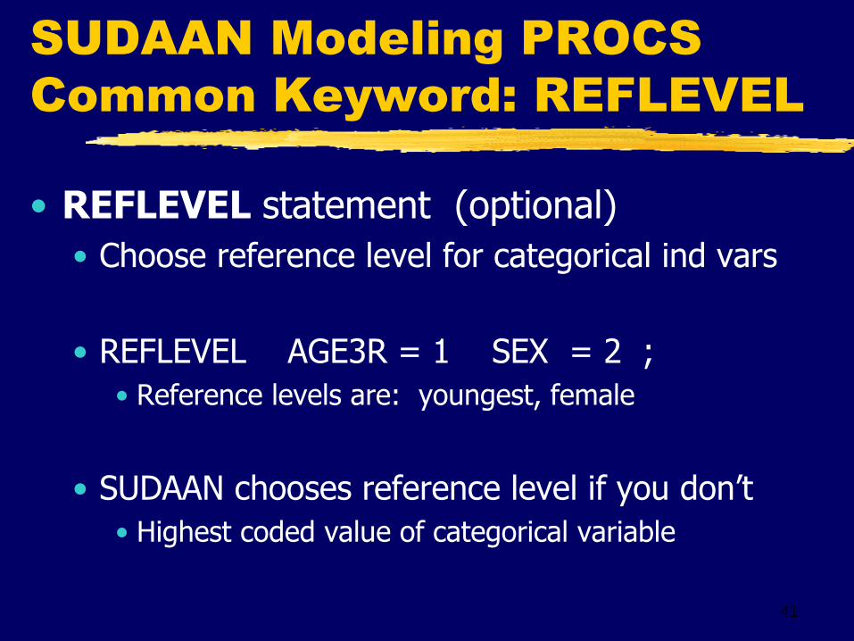
• REFLEVEL statement (optional)

• Choose reference level for categorical ind vars

• REFLEVEL AGE3R = 1 SEX = 2 ;

• Reference levels are: youngest, female

• SUDAAN chooses reference level if you don’t

• Highest coded value of categorical variable

42


Common Keyword: CONTRAST

• CONTRAST statement (optional)

• Linear contrast(s), a vector [1 df] or matrix [multiple df], which is then multiplied by the vector of popn regression coeffs

• Tests null hypothesis(es) about popn regr coeffs

• Many CONTRAST statements per PROC allowed

• SUDAAN outputs many default contrasts

• CONTRAST tedious to use! EFFECTS is easier!

43


Common Features: EFFECTS

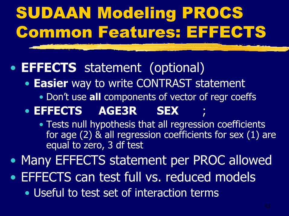
• EFFECTS statement (optional) • Easier way to write CONTRAST statement

• Don’t use all components of vector of regr coeffs

• EFFECTS AGE3R SEX ; • Tests null hypothesis that all regression coefficients

for age (2) & all regression coefficients for sex (1) are equal to zero, 3 df test

• Many EFFECTS statement per PROC allowed

• EFFECTS can test full vs. reduced models • Useful to test set of interaction terms

44


Common Keyword: TEST

• TEST options ; (5 keywords) • WALDCHI (Wald chi-square test, r df)

• WALDF (r, e ) = WALDCHI / r , e=ddf

• ADJWALDF ( function of WALDF)

• SATADJCHI (SRS with eigenvalues)

• SATADJF (SRS with eigenvalues)

• Specifies calculations to test hypotheses • Both default hyps & hyps that you specify

• TEST is optional: default is WALDF

45

More on Common Keyword:

TEST

• Default Waldf works well most times

• Adjwaldf & Satadjf better for small ddf

• Survey ddf = # of PSUs – # of strata

• NHANES surveys smaller ddf: 30, 49, …

• Survey ddf large for BRFSS statewide

• Because each sample adult is a PSU (for DSS)

• Waldchi too liberal for small ddf

• DB advice: avoid using Waldchi (if possible)

46

MODELING PROCEDURES

SAS SURVEY PROCS

Overview

47

3 SAS Modeling PROCS for

Survey Data Analysis

• SurveyLogistic--logistic regression +

• Dep Var dichotomous or > 2 levels

• Ind Vars—continuous/categorical

• SurveyReg--linear regression

• Dep Var continuous

• Ind Vars—continuous/categorical

• SurveyPHReg-Cox proportional hazards regression (survival) analysis

48

SAS SurveyLogistic: LINK

option on MODEL Statement

• LINK = LOGIT (or CLOGIT, CUMLOGIT) • Logit or Cumulative logit model ( default)

• Dependent variable at 2 or more levels

• LINK = GLOGIT • Generalized logit function (dep var >=2 levels)

• LINK = CLOGLOG • Binary complementary log-log model or

cumulative complimentary log-log model

• LINK = PROBIT

49

SAS SurveyLogistic

• Wald chi-square test statistic: hypotheses • Recall: too liberal for small survey ddf!

• MODEL statement: specify level of binary variable for which probability is modeled • SAS may not choose level that YOU want

• Choose how to parameterize cat ind vars

• Many methods, including reference group

• Default is EFFECT (likely not what you want)

• Specify on CLASS statement

50

SAS

SurveyReg

• Similar to nonsurvey SAS PROC GLM

• SAS chooses how parameterize cat ind vars

• Reference group method

• SAS orders levels of cat var & chooses last level as reference group (formatted, internal, etc.)

• May not be level you want for reference!

• Wald F test used to test default hypotheses & requested contrasts (only option) • Wald F default test in SUDAAN modeling procs

51

Common Features in

SurveyLogistic & SurveyReg

• MODEL Y = X1 X2 X3 X1*X2 ;

• One model statement per PROC

• CLASS Specify categorical ind vars

• Remaining ind vars assumed continuous

• X1*X2 acceptable for:

• 2 continuous vars, 1 cont & 1 cat, 2 cat vars

• X1*X1 also works for X1 continuous

52

Common Features in

SurveyLogistic & SurveyReg

• Contrast and Estimate statements-as GLM

• Estimate & test own combination of regr coeffs

• Test statement: also test null hypotheses

• New statements in SAS 9.3

• Effect: make new ind vars for model

• LSMeans

• LSMEstimate

• Note: SAS Effect statement not same as SUDAAN Effect statement

53

LOGISTIC REGRESSION

SUDAAN PROC LOGISTIC

SAS PROC SURVEYLOGISTIC

Dichotomous dependent variable

54

LOGISTIC REGRESSION

Review

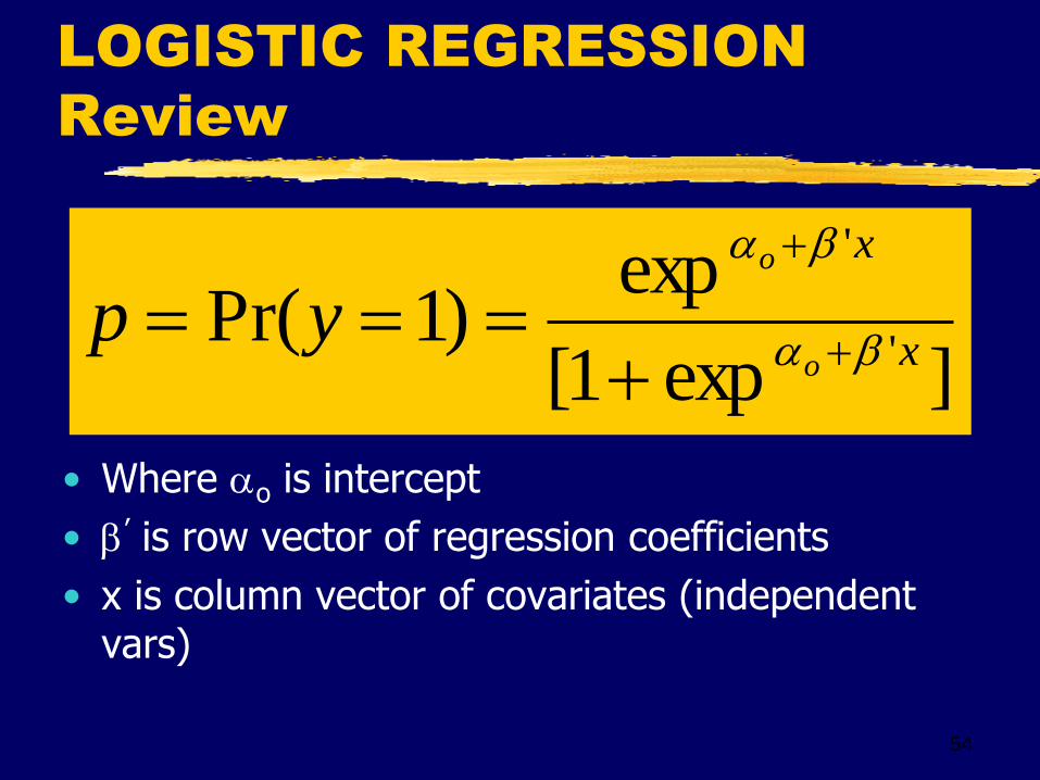
• Where o is intercept

• ’ is row vector of regression coefficients

• x is column vector of covariates (independent vars)

]exp1[

exp)1Pr(

'

'

x

x

o

o

yp

55

LOGISTIC REGRESSION

Review

1exp ratio odds

x odds ln

'exp)0Pr(

)1Pr(

xoy

yodds

Logistic Regression

Example

Consider Various Models

Only 3 Independent Variables

56

Logistic Regression

Example

• Dependent = Binge Drinking (old defn)

• Binge01, 1=drinker, 0=not

• Sex & Race4 : 2 categorical ind vars

• Age: use as continuous or categorical?

• First, do bivariate analysis to confirm relationship of each ind var to binge

57

LecEx07

Crosstab & SurveyFreq

• Tables (Race4 Sex AgeDec Sex*Race4) * Binge01 ;

• Results: Binge drinking related to:

• 1. Sex: males higher prevalence

• 2. Age: prevalence declines with higher age

• 3. Race/ethnicity: BNH lower? Hisp higher?

58

Decisions about Age in

Logistic Regression Model

• Age categorical or continuous?

• Fewer parameters to estimate if continuous

• Continuous age linear, quadratic, higher?

• Center age? Yes, if…..

• Age=0 not in dataset ( 18 thru 97)

• Intn of Age with race or sex, or age quadratic

• How center? Range midpoint = 57.5

• AgeL57 = Age – 57.5

59

60

LecEx 8A SUDAAN

Main Effects Model - 6 coeffs

• Proc RLogist

• Class Race4 Sex ;

• Model Binge01 = Sex Race4 AgeL57 ;

• Reflevel Sex = 2 Race4 = 1 ;

• Test WaldF WaldChi ; why 2?

• Print ; /* default printout */

• Print / HLTest = ALL ; for GOF

61

Count # Regression Coeffs

for This Model = 6

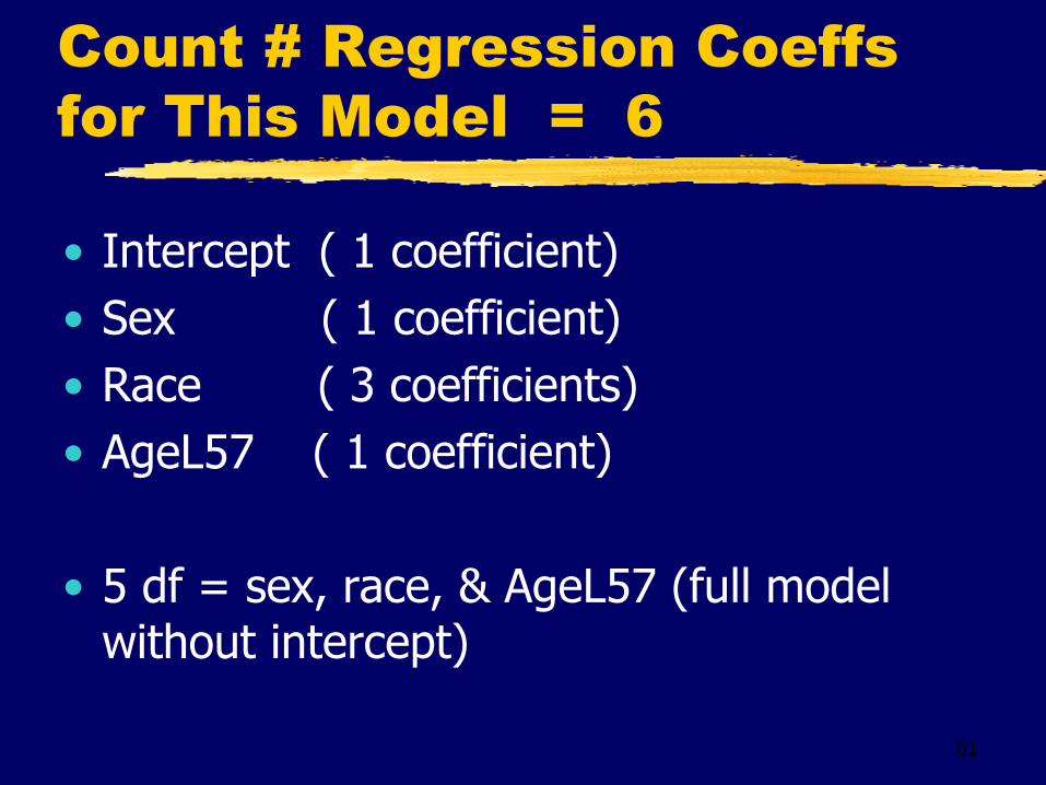
• Intercept ( 1 coefficient)

• Sex ( 1 coefficient)

• Race ( 3 coefficients)

• AgeL57 ( 1 coefficient)

• 5 df = sex, race, & AgeL57 (full model without intercept)

62

LecEx 8A SUDAAN

EFFECTS Statement

• Effects Sex / name = “DB Test for Main Effect of Sex” ;

• Effects Race4 / name = “DB Test for Main Effect of Race/Ethnicity” ;

• Effects AgeL57 / name = “DB test for Main Effect of AgeL57” ;

63

Hosmer Lemeshow GOF

SUDAAN RLOGIST

• Use Wald chi-square to test model effects:

• HL GOF p-value = 0.1733

• Use Wald F test to test model effects:

• HL GOF p-value = 0.1721

• Main effects model looks plausible

• No GOF test in SAS SurveyLogistic

64

LecEx 8B Logistic Regr

SAS SurveyLogistic

• Proc SurveyLogistic NoMcar data =

• Class sex (ref=‘2=female’) race4 (ref=‘1=WNH’) / param = ref ;

• Model binge01 (Event = ‘1=yes’) = sex race4 AgeL57 ;

• Units age = 1 5 10 ;

LecEx 8B Logistic Regr

SAS SurveyLogistic

• Contrast 'sex effect 1 df' sex 1 ;

• Contrast 'age effect 1 df' AgeL57 1 ;

• Contrast 'race effect 3 df' race4 1 0 0 , race4 0 1 0 , race4 0 0 1 ;

65

66

Compare Answers 8A & 8B

RLOGIST & SURVEYLOGISTIC

• Point estimates of popn regression coeffs and odds ratios: exactly same

• Estimated s.e. of estimated regr coeffs & odds ratio CI: very close or same

• Wald chi-square statistics: very close

• P-values: very close or same

• Item nonresponse method same: NoMcar

67

Interpretation of Main

Effects Model: Example 8

Effect Regr p-value OR CI on OR

AgeL57 -0.04 <.0001 0.96 .95,.96

Male 1.36 <.0001 3.89 3.2, 4.7

BNH -0.61 <.0001 0.54 .42, .69

Hisp 0.13 .63 1.13 .68, 1.89

OtherNH -0.43 .08 0.65 .40, 1.05

Alternate Program to 8B with

AgeL57, Pgm 8C with Effect

• One option on Effect is Polynomial

• Several options under Polynomial

• Effect AgePoly1C = polynomial ( age / degree = 1 details

standardize ( method = range ) = center ) ;

• Model Binge01 (Event = ‘1=yes’) = sex race4 AgePoly1C ;

68

Compare Pgs 8B & 8C with

SAS SurveyLogistic

• Outputs 8B & 8C same answers, except…

• 8C does not give odds ratio for constructed effect AgePoly1C

• Whereas 8B gives odds ratio for dataset variable AgeL57

69

70

Include a Quadratic Term for

Age? LecEx09Q

• Model so far: Sex, Race4, AgeL57

• 9QA. Sudaan RLogist with AgeL57sq

• 9QB. SAS SurveyLogistic with AgeL57sq or with AgeL57 * AgeL57

• 9QC. SAS SurveyLogistic: Effect Poly (age) to add linear & quadratic centered age

• Conclusion: not obvious that quadratic term needed. Forget it for now.

71

Do We Need to Include

Interaction Terms in Model?

• Main effects model may be OK • H-L test not terribly suspicious (p=.1721)

• Investigate if interactions needed

• 1st, model with all possible interactions • Three 2-factor interactions

• Sex * race4, sex * AgeL57, race4 * AgeL57

• One 3-factor interaction sex*race4*AgeL57

• All interaction terms: 10 popn regr coeffs

• 10 df custom contrast: all 10 coeffs = zero

72

LecEx 9A SUDAAN Logistic

All intns: total 16 regr coeffs

• PROC RLOGIST ………

• CLASS SEX RACE4 ;

• MODEL Binge01 = Sex Race4 AgeL57 Sex * Race4 Sex * AgeL57 Race4 * AgeL57 Sex * Race4 * AgeL57 ;

• REFLEVEL Sex = 2 Race4 = 1 ;

• TEST WaldF WaldChi ;

73

LecEx 9A SUDAAN Logistic

All intns: 16 regr coeffs (cont)

• PRINT ; /* default printout */

• PRINT / HLTest = ALL ;

• Effects Sex * Race4 Sex * AgeL57 Race4 * AgeL57 Sex * Race4 * AgeL57 / Name = “Test all Interactions 10 df” ; • Easy way to write CONTRAST statement

• Don’t need to deal with 30 positions in regr coefficient vector (16 + 14 defined as zero)

74

LecEx 9B All Intns.

SurveyLogistic: 16 coeffs

• Proc surveylogistic data =


• Model binge01 (EVENT=‘1=yes’) = sex race4 ageL57 sex * race4 sex * ageL57 race4 * ageL57 sex * race4 * ageL57 ;

75

LecEx 9B

SurveyLogistic: CONTRAST

• Contrast '10 df interaction test'

sex * race4 1 0 0 ,

sex * race4 0 1 0 ,

sex * race4 0 0 1 ,

sex * ageL57 1 ,

76

LecEx 9B (cont)


Race4 * AgeL57 1 0 0 ,

Race4 * AgeL57 0 1 0 ,

Race4 * AgeL57 0 0 1 ,

Sex * Race4 * AgeL57 1 0 0 ,

Sex * Race4 * AgeL57 0 1 0 ,

Sex * Race4 * AgeL57 0 0 1 ; run ;

77

LecEx 10

Consider a Reduced Model

• Three factor interaction seems not needed

• Model now with three 2-factor interactions

• Sex * race4, sex * age, race4 * age

•

• 7 df custom contrast: all 7 coeffs = zero

78

LecEx 10A

SUDAAN: 13 regr coeffs

• PROC RLOGIST ………

• Class SEX RACE4 ;

• Model Binge01 = Sex Race4 AgeL57 Sex * Race4 Sex * AgeL57 Race4 * AgeL57 ;

• RefLevel Sex = 2 Race4 = 1 ;

• Test WaldF WaldChi ;

79

LecEx 10A (cont)

SUDAAN: 13 regr coeffs

• PRINT ; /* default printout */

• PRINT / HLTest = DEFAULT ;

• Effects Sex * Race4 Sex * AgeL57 Race4 * AgeL57 / NAME = “Interaction test with 7 df” ;

80

LecEx 10B

SurveyLogistic: 13 coeffs



• Model binge01 (Event=‘1=yes’) = sex race4 AgeL57 sex * race4

AgeL57 * sex AgeL57 * Race4 ;

81

LecEx 10B (cont)


• Contrast ‘7 df interaction test'

Sex * Race4 1 0 0 ,

Sex * Race4 0 1 0 ,

Sex * Race4 0 0 1 ,

AgeL57 * Sex 1 ,

AgeL57 * Race4 1 0 0 ,

AgeL57 * Race4 0 1 0 ,

AgeL57 * Race4 0 0 1 ;

82

Model Conclusions So Far

• Main effects model (ex 8) maybe OK

• Model with all interactions (ex 9)

• 3-factor interaction not needed

• Model with all 2-factor interactions (ex 10)

• 2-factor intn Race4 * age may be needed

• Next step: include three 2-factor intns & test null hypothesis that sex * ageL57 & sex * race4 not needed in model

83

LecEx11A SUDAAN

13 coeffs, EFFECTS

• PROC RLOGIST.. ;

• Class SEX RACE4 ;

• Model Binge01 = Sex Race4 AgeL57 sex * race4 sex * ageL57

race4 * ageL57 ;

• Effects sex * race4 sex * ageL57 / name = “Intn Test with 4 df” ;

84

LecEx 11B 13 coeffs

SurveyLogistic



• Model binge01 (Event=‘1=yes’) = sex race4 ageL57 sex*ageL57 race4*ageL57 ;

• Contrast ‘4 df interaction test'

Sex * AgeL57 1 , Sex*Race4 1 0 0 ,

Sex*Race4 0 1 0 , Sex*Race4 0 0 1 ;

85

LecEx 12A SUDAAN

Only one interaction

• PROC RLOGIST.. ;


• MODEL Binge01 = SEX RACE4 AgeL57 race4 * ageL57 ;

• H-L GOF test: fit seems OK (p = .2140)

• Race4* ageL57 p-value: .0011

• SUDAAN prints out “odds ratios” not relevant, i.e. ones with race4 or ageL57

86

LecEx 12B only one intn

SurveyLogistic



• MODEL binge01 (Event=‘1=yes’) = sex race4 ageL57 race4*ageL57 ;

• SAS prints out only one OR, for sex:

3.92 ( 3.25, 4.71)

2 Candidates for Logistic

Regression Model So Far

• Main effects model (HL p-value = .172)

• Sex, Race4, AgeL57

• Simpler, no interactions

• Usual interpretation of odds ratios

• Model with 1 intn term (HL p-value = .214)

• Sex, Race4, AgeL57, Race4 * AgeL57

• More difficult to interpret

• Interaction appears stat sign, makes sense

87

How Summarize Model with

the Intn? Use Odds Ratios

• Sex OR = 3.92, easy

• Race/Ethnicity odds ratios

• ORs for AgeL57=0, i.e. age = 57.5 years

• Sudaan output, not SAS

• Race ORs for other values of age: can program

• Age odds ratio (1 or more years)

• OR in output for NHW

• Age OR for other Race/Eth: can program

88

Disadvantages of Presenting

Results Using Odds Ratios

• Not direct to get software to do the calculations for you (although possible)

• Must present many odds ratios

• Age OR for 3 levels of race/ethnicity

• Race/Eth ORs for several values of age

• Odds ratios exaggerate strength of relationship if outcome prevalence not rare

89

Another Way to Present

Results of Model with Intn

• Use predicted marginals

• Use prevalence ratios (not odds ratios)

• Advantages:

• Results in terms of probabilities, not OR

• More concise than reporting many ORs

90

91

PREDICTED MARGINALS

PREDICTED RISK RATIOS

For Logistic Regression

SUDAAN only

Useful in main effects models or

those with interaction(s)

Predicted Marginals

Logistic Regression

• Assume categorical independent variable at four levels, e.g. race/ethnicity

• Assume level 1 is reference level (WNH)

• Four regression coefficients for this variable are:

• Other variables in model (e.g. age, sex)

• Model could also have interactions

92

1 2 3 4( 0), , ,and

93

Calculate Predicted Marginal

for Level 1 of Categorical Var

• Assign each sample obsn in model the value of level 1(WNH) for categorical variable

• Use fitted model to predict, for each sample obsn in model, probability that y = 1 • Use covariate vector xi for that obsn

• Take weighted average of these predicted probabilities over sample obns in model

• This is predicted marginal for level 1

94

Predicted Prob: Sample Obsn

i at Level 1 of Race/Eth (WNH)

0

0

0

10

1 1

1

'

'

expPr( | )

[ exp ]

i

i

x

i ix

p y level

95

Predicted Marginal: Level 1

(WNH) of Categorical Variable

1 1

1 1

1 1Pr( | ) /i r i r

i i i

i i

p y level w p w

96

Predicted Marginal:Level 2

(BNH) of Categorical Variable

0 2

0 2

2

2 2

1 1

1 2

1

'

'

expPr( | )

[ exp ]

/

i

i

x

i ix

i r i r

i i i

i i

p y level

p w p w

97


(Hisp) of Categorical Variable

0 3

0 3

3

3 3

1 1

1 3

1

ˆ '

ˆ '

expPr( | )

[ exp ]

/

i

i

x

i ix

i r i r

i i i

i i

p y level

p w p w

98


(OthNH) of Categorical Variable

0 4

0 4

4

4 4

1 1

1 4

1

ˆ '

ˆ '

expPr( | )

[ exp ]

/

i

i

x

i ix

i r i r

i i i

i i

p y level

p w p w

99

Predicted Marginal

• The column vector for sample obsn i is not considered to be “fixed”

• I.e. it has sampling variance

• Assumption to obtain s.e. for each predicted marginal

• Probably realistic assumption in human population sample surveys

• Which is why some survey data analysts prefer predicted marginals over conditional marginals

ix

100

Predicted Marginal

How to Think About It

• Estimate logistic regression model for popn, with ind categorical var of interest

• For each sample obsn i in model, use model to predict prob of outcome “as if” obsn was assigned to level 1 of cat var & all other covariate values are what they are for that obsn

• Now assign that same sample obsn to level 2 of cat var, & use model to predict outcome prob

• Continue with remaining levels of cat var

• Conceptually, a way of standardizing on cat var

101

Why Korn & Graubard Like

Predicted Marginals

• Results are probabilities rather than regression coefficients or odds ratios

• The probabilities are adjusted for other variables in the model

• Convey scale of differences between levels of a cat var better than regression coefficients or odds ratios do

• Easier to see effect of interactions between the cat var and a covariate

102

Why Korn & Graubard Like

Predicted Marginals (cont)

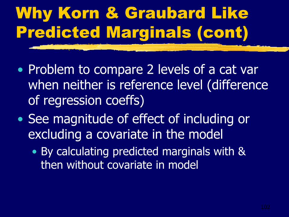
• Problem to compare 2 levels of a cat var when neither is reference level (difference of regression coeffs)

• See magnitude of effect of including or excluding a covariate in the model

• By calculating predicted marginals with & then without covariate in model

103

Some References on

Predicted Margins

• Graubard & Korn “Predictive Margins….”

• Biometrics, 1999, vol 55, 652-659

• Korn & Graubard, Analysis of Health Surveys

• John Wiley, 1999, Chapter 3

• SUDAAN Language Manual, Release 10 or 11

• Excellent applied paper: Potosky, Breen, Graubard, Parsons: cancer screening & health insurance, Medical Care, 1998.

Predicted Risk Ratios

SUDAAN, new in Release 10

• Logistic regression

• Calculate predicted marginals for a categorical variable

• Choose one level of categorical variable as reference level

• For each other level, take ratio of predicted marginal of level to predicted marginal of reference level

104

Definition of Predicted Risk

Ratios

• Categorical variable at 4 levels, e.g. Race4

• Predicted marginals:

• Predicted risk ratios (level 1 is reference)

105

1 2 3 4ˆ ˆ ˆ ˆ, , , p p p and p

32 42 3 4

1 1 1

ˆˆ ˆ, ,

ˆ ˆ ˆ

pp prr rr rr

p p p

Why Use Predicted Risk

Ratios (or Prev Ratios)

• Idea analagous to odds ratios

• But risk ratio is ratio of probabilities (prev or risk), & probabilities adjusted for all other covariates in the model

• Note: for common health outcomes, OR always larger than risk or prevalence ratio, sometimes substantially

• OR may exaggerate strength of association

106

107

LecEx13A SUDAAN

Ask for Predicted Marginals

• proc RLOGIST data = …………

• MODEL binge01 = SEX RACE4 AgeL57

RACE4 * AgeL57 ;


• REFLEVEL sex = 2 race4 = 1 ;

• PREDMARG RACE4 SEX ;

• predmarg ageL57 / ageL57 = 7.5 -2.5 -12.5 -22.5 -32.5 ; /* Choose values for cont age */

108

LecEx13B SUDAAN

Ask for Predicted Risk Ratios

• proc RLOGIST data = …………

• Model binge01 = SEX RACE4 AgeL57

RACE4 * AgeL57 ;

• Class Sex Race4 ;

• RefLevel sex = 2 race4 = 1 ;

• PredMarg Race4(1) Sex(2) / adjrr ;

• PredMarg ageL57 (-32.5) / ageL57 = 7.5 -2.5 -12.5 -22.5 -32.5 ;

LecEx13 Est. Pred Margs &

Risk(Prev) Ratios: Intn Model

Ind. Var. Pred Marg s.e. PredMrg Risk Ratio CI RiskRatio

Male .2176 .01 3.04 (2.61, 3.55)

Female .0715 .005 Ref Ref

WNH .1637 .007 Ref Ref

BNH .1043 .009 0.64 (.53, .77)

Hisp .1790 .03 1.09 (.76, 1.57)

OtherNH .1166 .02 0.71 (.48, 1.05)

Age=25 .2428 .011 Ref Ref

Age=35 .1765 .007 0.73 (.70, .76)

Age=45 .1245 .005 0.51 (.47, .56)

Age=55 .0861 .005 0.35 (.31, .41)

109

110

LecEx13C SUDAAN No Intn

Pred Margs & Prev Ratios

• Compare Main Effects model to model with intn

• proc RLogist data = …………

• Model binge01 = Sex Race4 AgeL57 ;

• Class Sex Race4 ;

• RefLevel sex = 2 race4 = 1 ;

• PredMarg Race4 Sex / adjrr ;

• PredMarg ageL57 (-32.5) / ageL57 = 7.5 -2.5 -12.5 -22.5 -32.5 ;

Compare Model with Intn to

Model with No Intn

PrdMrg Intn

PrdMrg No Intn

PrevRatio Intn

PrevRatio No Intn

OR No Intn

Male .2176 .2177 3.04 3.05 3.89

Female .0715 .0714 Ref Ref Ref

WNH .1637 .1626 Ref Ref Ref

BNH .1043 .1004 0.64 0.62 0.54

Hisp .1790 .1783 1.09 1.10 1.13

OtherNH .1166 .1167 0.71 0.72 0.65

Age=25 .2428 .2399 Ref Ref

Age=35 .1765 .1747 0.73 0.73 10yr=0.65

Age=45 .1245 .1235 0.51 0.51

Age=55 .0861 .0852 0.35 0.36

Age=65 .0590 .0577 0.24 0.24 111

112

Estimation of Odds Ratios

with Interactions in Model

Interaction term contains

one categorical variable and

one continuous variable

Dealing with a two-way

interaction in Logistic Model

• Use model of LecEx12: Race4*AgeL57

• For each level of Race4, estimate age regression coefficient & odds ratio for 1 (or more) year(s) increase in age

• For selected values of AgeL57, estimate 3 odds ratios for race/ethnicity

• Program these calculations in SUDAAN RLogist and SAS SurveyReg

113

LecEx14A SUDAAN RLOGIST

Age Regr Coeff & OR, by Race4

• Model Binge01 = Sex Race4 AgeL57 Race4 * AgeL57 ; /* age continuous */

• Effects AgeL57 / Race4 = 1 exp name= "Age Effect & Age OR, WNH" ;

• Effects statement tests null hyp: popn age regr coeff for WNH = zero. Estimated age regr coeff for WNH is exponentiated to give age OR for WNH.

114



• Effects ageL57 / Race4= 2 exp name = "Age Effect & Age OR, BNH" ;

• Effects ageL57 / Race4= 3 exp name= "Age Effect & Age OR, Hisp“;

• SUDAAN not print estimated regr coeff for age for each level of Race4

115

LecEx14B SAS SurveyLogistic



• Contrast 'WNH one year’ ageL57 1 / estimate = both ; /* regr coeff + OR*/

• Contrast 'WNH ten years' ageL57 10 /

• estimate = exp ; /* OR only */

• Above statements work because WNH is reference level for Race4

116



• Contrast 'BNH one year'

ageL57 1 race4 * ageL57 1 0 0 / estimate = both ;

• Contrast 'BNH ten years'

ageL57 10 race4 * ageL57 10 0 0 / estimate = exp ;

117



• Contrast ‘Hisp one year'

ageL57 1 race4 * ageL57 0 1 0 / estimate = both ;

• Contrast ‘Hisp ten years'

ageL57 10 race4 * ageL57 0 10 0 / estimate = exp ;

118

Estimated OR & CI for binge

drink: 10 year age increase

• WNH: .60 ( .56, .65 ) SurveyLogistic

• BNH: .80 ( .71, .90 ) & Sudaan

• Hisp: .66 ( .47, .92 )

• OthNH: .65 ( .47, .91 )

• BNHs differ from WNHs on age regr coeff

• (1 df default test)

• Age ORs larger for BNH than for WNH

• Probably because BNH binge prevalence lower 119

Recap: Estimating Odds

Ratios with Intn in Model

• LecEx14. Race4 * AgeL57 interaction

• Estimate age effect at each level of Race4

• Sudaan Logist or SAS SurveyLogistic

• Conclusion: BNHs different age effect

• LecEx15. Race4 * AgeL57 interaction

• Estimate Race effect for varying values of age

• Sudaan Effects statement: not work!

• Can be done in SAS SurveyLogistic

120


• Not able to use SUDAAN EFFECTS statement for following two calculations:

• 1. 3 df test for Race4 at a chosen level of age

• 2. Three race/ethnicity odds ratios for a chosen level of age

• Seems cannot condition on value for a continuous variable when using EFFECTS statement in SUDAAN

121


Race/Ethnicity ORs, by AGE


• Contrast 'BNH/WNH OR age = 25'

race4 1 0 0 Race4 * ageL57 -32.5 0 0 / estimate = exp ;

122


Race/Ethnicity ORs, by AGE

• Contrast 'Hisp/WNH OR age = 25'

race4 0 1 0 Race4 * ageL57 0 -32.5 0 / estimate = exp ;

• Contrast 'OthNH/WNH OR age = 25' race4 0 0 1 Race4 * ageL57 0 0 -32.5 / estimate = exp ;

123


Race Effect, by AGE

• Contrast '3 df test of effect of Race4 at AGE = 25'

race4 1 0 0 Race4 * ageL57 -32.5 0 0 ,

race4 0 1 0 Race4 * ageL57 0 -32.5 0,

race4 0 0 1 Race4 * ageL57 0 0 -32.5 ;

124

15B Results: Effect of & ORs

for Race/Eth at a Given Age

• Effect of race/ethnicity is stat significant for ages 25, 35 & 45 but not for 55 & 65

• Race/ethnicity ORs for ages 55 & 65 have CIs that all include 1.0

• Age 25, BNH/WNH OR = .39 ( .28, .54 )

• Age 35, BNH/WNH = .52 ( .41, .66)

• Age 55, BNH/WNH = .91 ( .68, 1.22)

125

Extensions of Workshop

Examples on Interactions

• Two way interaction: between 2 vars but both categorical, rather than one categorical & one continuous

• Can be done in both RLogist and SurveyLogistic: syntax similar to examples here, but some differences

• 3 way interaction: likely complicated

• Predicted marginals perhaps only path

126

Linear Regression

Sudaan Regress

SAS SurveyReg

127

A Few Comments on

Linear Regression

• Few continuous dep vars in BRFSS

• BMI, # cigs smoked per day

• Statements illustrated today in RLogist & in SurveyLogistic can be useful

• Sudaan: Effects, Contrast,

• SAS: Effect, Contrast, Estimate

• Easier, since is a linear model

128

129

REFERENCES

References on Sample

Survey Design and Analysis

130

Recommended Books:

Surveys & Their Analysis

• Heeringa, Steven, BT West, PA Berglund. Applied Survey Data Analysis, Chapman & Hall/CRC, Boca Raton, FL, 2010. Excellent. $84 list.

• Groves, Robert et al, Survey Methodology, 2nd edn., John Wiley, 2009, paper, $85 list.

• Introduction/overview of all aspects of surveys

• Korn, Edward & Barry Graubard, Analysis of Health Surveys, John Wiley, 1999. $165 list.

• Strategies for survey data analysis, math-stat useful

131

Recommended Books:

Sampling Methods & Analysis

• Lee, Enu Sul & Robert Forthofer. Analyzing Complex Survey Data, 2nd edn, 2006, Sage Publs.

• Short, concepts oriented, condensed Korn/Graubard

• Lohr, Sharon. Sampling: Design and Analysis. 2010, Brooks/Cole, Cengage Learning.

• Applied introduction to sampling (algebra)

• Clear explanations and real-life examples

• Cochran, William G. Sampling Techniques: 3rd Edition. 1977, John Wiley. Math-stat.

132

Some Useful WEB Sites

• http://www.amstat.org/sections/srms • ASA, Survey Research Methods Section

• What Is A Survey? booklets excellent

• http://www.hcp.med.harvard.edu/statistics/survey-soft/ Software for survey data

• http://www.aapor.org . Go to Resources & Education, then Researchers, then: Best Practices, Standard Definitions Response Rate (2011), Poll/Survey FAQ. Excellent discussions.

http://www.amstat.org/sections/srms

http://www.hcp.med.harvard.edu/statistics/survey-soft/




http://www.aapor.org/

133

Special Issues of Public

Opinion Quarterly

• Vol. 70, No. 5, 2006. “Special Issue: Nonresponse Bias in Household Surveys”

• Vol. 71, No. 5, 2007. “Special Issue: Cell Phone Numbers & Telephone Surveying in U.S.

• Vol. 74, No.5, 2010. “Special Issue: Total Survey Error”

• http://www.oxfordjournals.org/our_journals/poq/collectionspage.html PH Survey Methods

http://www.oxfordjournals.org/our_journals/poq/collectionspage.html

http://www.oxfordjournals.org/our_journals/poq/collectionspage.html

Some Survey Research

Journals

• Survey Methods: Insights from the Field. http://surveyinsights.org/ (electronic)

• Journal of Survey Statistics & Methodology. http://www.oxfordjournals.org/our_journals/jssam/

• Survey Methodology. http://www.statcan.gc.ca/ads-annonces/12-001-x/index-eng.htm

134

http://surveyinsights.org/

http://www.oxfordjournals.org/our_journals/jssam/

http://www.oxfordjournals.org/our_journals/jssam/

http://www.statcan.gc.ca/ads-annonces/12-001-x/index-eng.htm









135

Lab Exercise

Logistic Regression

• Dependent variable: Diabetes yes or no

• Independent vars: age, race/eth, sex, any other variables of interest in dataset

• Develop a logistic regression model

compare sudaan & sas for brfss modeling analyses€¦ · compare sudaan & sas for brfss...

Documents