application of the sudaan software package to clustered...
TRANSCRIPT

Application of the SUDAAN Software Package®
to Clustered Data Problems:
Pharmaceutical Research
by
Gayle S. BielerRick L. Williams
Research Triangle Institute
Prepared for:New Jersey Chapter of the ASA
May 12, 1997
Originally presented to:US Food and Drug Administration
Washington, DCFebruary 9 and June 21, 1996
1996 Joint Statistical MeetingsComputer Technology Workshop
Chicago, IllinoisAugust, 1996

Application of the SUDAAN Software Package to Clustered Data Problems inPharmaceutical Research was written by Gayle S. Bieler and Rick L. Williams
Copyright 1997 by Research Triangle InstituteP.O. Box 12194Research Triangle Park, NC 27709-2194
All rights reserved. No part of this publication may be reproduced or transmitted by anymeans without permission from the publisher.
SUDAAN and RTI are trademarks of the Research Triangle Institute.SAS is a trademark of SAS Institute, Inc.

68'$$1Software for the Statistical Analysis of Correlated Data
Application of the SUDAAN Software Package®
to Clustered Data Problems:
Pharmaceutical Research
Gayle S. [email protected]
Rick L. [email protected]
Research Triangle Institute
Prepared for:New Jersey Chapter of the ASA
May 12, 1997
Originally presented to:US Food and Drug Administration
February 9 and June 21, 1996
1996 Joint Statistical MeetingsChicago, Illinois
August, 1996
Research Triangle InstitutePO Box 12194Research Triangle Park, NC 27709-2194

Application of the SUDAAN Software Package to Clustered DataProblems: Pharmaceutical Research
Table of Contents
Presentation Notes . . . . . . . . . . . . . . . . . . . . . . . . . . . . . . . . . . . . . . . . . . . . . . . . . . . . . . . 1-63
References . . . . . . . . . . . . . . . . . . . . . . . . . . . . . . . . . . . . . . . . . . . . . . . . . . . . . . . . . . . . 64-68
Appendix I: Abstracts from Related Papers . . . . . . . . . . . . . . . . . . . . . . . . . . . . . . . . . . . 69-76
Appendix II: Examples Using the SUDAAN Software Package . . . . . . . . . . . . . . . . 79-185
Example 1. Teratology: Effect of the Compound DEHP on Fetal Death . . . . . 79-100
Example 2. Clinical Trials: Effect of Treatment on Repeated Exercise Timesto Angina Pectoris . . . . . . . . . . . . . . . . . . . . . . . . . . . . . . . . . . . . 101-130
Example 3. Clinical Trials: Comparison of Two Inhaler Devices in aCross-Over Clinical Trial . . . . . . . . . . . . . . . . . . . . . . . . . . . . . . . . 131-160
Example 4. Teratology: Effect of Boric Acid on Fetal Body Weight . . . . . . . 161-185
Appendix III: Comparisons to Other Methods . . . . . . . . . . . . . . . . . . . . . . . . . . . . . . . 188-194

ABSTRACT
In the pharmaceutical sciences, researchers often encounter data which are observed inclusters. Individual responses may represent multiple outcomes from the same patient (suchas sets of teeth, pairs of eyes, or longitudinal outcomes on the same individual) or frommultiple patients within a larger cluster, such as a physician clinic or an animal litter.Intracluster correlation, or the potential for clustermates to respond similarly, poses specialproblems for statistical analysis. This occurs because experimental units from the samecluster are not statistically independent. Failure to account for the cluster effect in thestatistical analysis can result in underestimated standard errors and false-positive test results.In addition, cross-over clinical trials will not yield the associated increase in statistical powerif the design is ignored in the analysis.
This seminar will describe the statistical methods used in SUDAAN and demonstrate its usevia a series of examples. The concept underlying the statistical methods is to fit marginalor population-averaged regression models (linear, logistic, multinomial logistic, andproportional hazards models) via Generalized Estimating Equations, treating the intraclustercorrelation as a nuisance parameter. Robust variances estimators (also known as sandwichestimators) ensure consistent variance estimates and valid inferences even when thecorrelation structure has been misspecified. The methods can also be used for descriptivedata analysis. Examples from clinical trials, teratology, and developmental toxicologyexperiments will be presented.
Presentation Notes 1
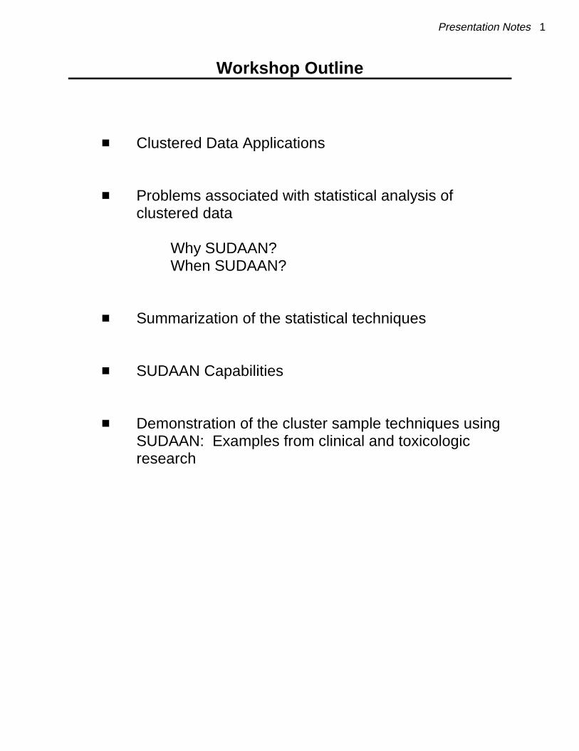
Workshop Outline
� Clustered Data Applications
� Problems associated with statistical analysis ofclustered data
Why SUDAAN?When SUDAAN?
� Summarization of the statistical techniques
� SUDAAN Capabilities
� Demonstration of the cluster sample techniques usingSUDAAN: Examples from clinical and toxicologicresearch

2 SUDAAN Applications
SUDAAN Procedures
DESCRIPTIVE PROCEDURES REGRESSION PROCEDURES
CROSSTAB REGRESSComputes frequencies, percentage Fits linear regression models and performsdistributions, odds ratios, relative risks, and hypothesis tests concerning the modeltheir standard errors (or confidence parameters; uses GEE to efficientlyintervals) for user-specified cross- estimate regression parameters, withtabulations, as well as chi-square tests of robust and model-based varianceindependence and the Cochran-Mantel- estimation.Haenszel chi-square test for stratified two-way tables.
DESCRIPTComputes estimates of means, totals, model parameters; also estimates oddsproportions, percentages, geometric ratios and their 95% confidence intervalsmeans, quantiles, and their standard for each model parameter.errors; also computes standardizedestimates and tests of single degree-of-freedom contrasts among levels of acategorical variable.
RATIOComputes estimates and standard errors their 95% confidence intervals for eachof generalized ratios of the form *y / *x, model parameter; uses GEE to efficientlywhere x and y are observed variables; estimate regression parameters, withalso computes standardized estimates and robust and model-based variancetests single-degree-of-freedom contrasts estimation.among levels of a categorical variable.
LOGISTICFits logistic regression models to binarydata and computes hypothesis tests for
MULTILOG Fits multinomial logistic regression modelsto ordinal and nominal categorical dataand computes hypothesis tests for modelparameters; estimates odds ratios and
SURVIVALFits discrete and continuous proportionalhazards models to failure time data; alsoestimates hazard ratios and their 95%confidence intervals for each modelparameter.
Presentation Notes 3
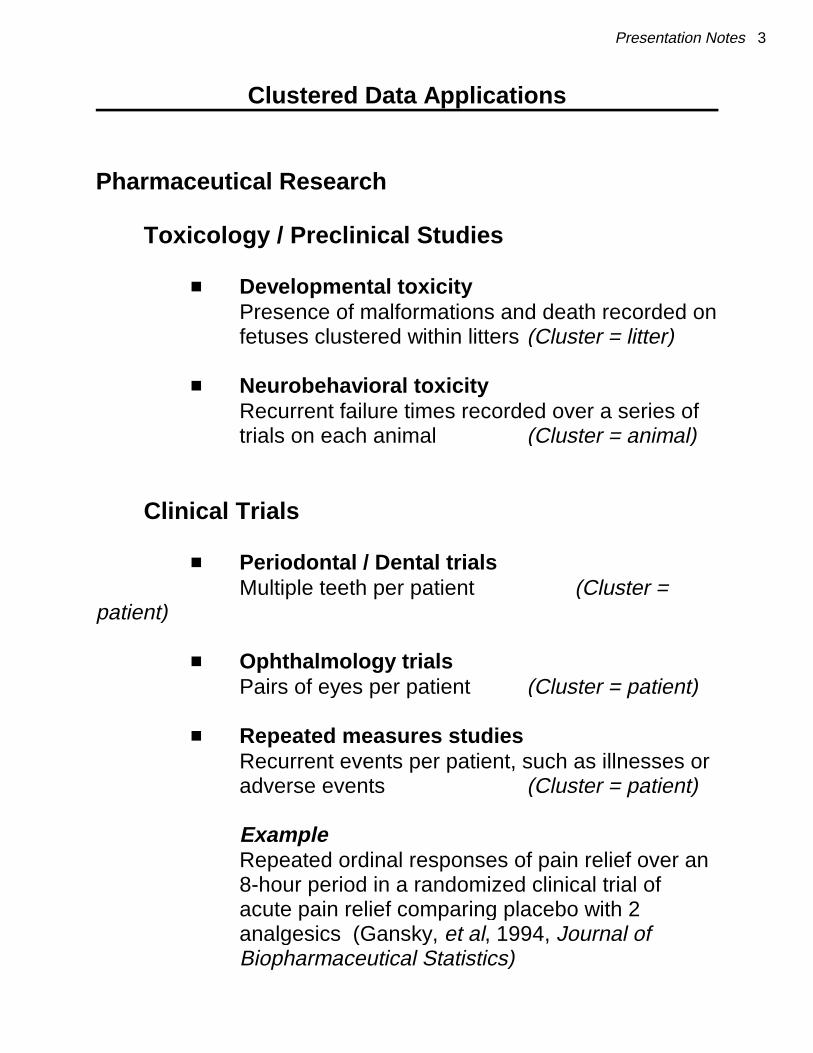
Clustered Data Applications
Pharmaceutical Research
Toxicology / Preclinical Studies
� Developmental toxicity Presence of malformations and death recorded onfetuses clustered within litters (Cluster = litter)
� Neurobehavioral toxicityRecurrent failure times recorded over a series oftrials on each animal (Cluster = animal)
Clinical Trials
� Periodontal / Dental trialsMultiple teeth per patient (Cluster =
patient)
� Ophthalmology trialsPairs of eyes per patient (Cluster = patient)
� Repeated measures studiesRecurrent events per patient, such as illnesses oradverse events (Cluster = patient)
ExampleRepeated ordinal responses of pain relief over an8-hour period in a randomized clinical trial ofacute pain relief comparing placebo with 2analgesics (Gansky, et al, 1994, Journal ofBiopharmaceutical Statistics)

4 SUDAAN Applications
Clustered Data Applications
Pharmaceutical Research
Clinical Trials (continued)
� Cross-Over StudiesPatients receive each treatment in sequence(Cluster = patient)
Example:3-period, 3 treatment cross-over study (Snapinnand Small,1986, Biometrics):
Investigational drug, aspirin, and placeboadministered in sequence to headache sufferers; Patients rated each drug on scaleof 1-4 according to amount of painrelief.

Presentation Notes 5
Why Did We Bother Developing SUDAAN?
Intra-Cluster Correlation
� Potential for clustermates to respond similarly (geneticand environmental influences)
� Experimental units from the same cluster are notstatistically independent
� Usually results in overdispersion , or extra-variation inthe responses beyond what would be expected underindependence
� Negative correlations have the opposite effecti.e., underdispersion , or reduction in variance belowwhat would be expected under independence
� Other standard statistical packages (e.g., SAS ,®
SPSS ) do not uniformly address the correlated data®
problem in all analytical procedures
SAS mainly uses correlated data methods for discrete(GENMOD) and continuous (MIXED, GENMOD)outcomes in regression models, but not for descriptivedata analysis
SUDAAN also uses correlated data methods for:
- Means and percentages- Medians and percentiles- Odds ratios and relative risks- Chi-square tests of independence- Cochran-Mantel-Haenszel tests

6 SUDAAN Applications
Failure to account for the cluster effect usually leads to:
� Underestimated standard errors forparameters of interest (means,proportions, regression coefficients)
� Test statistics with inflated Type I errorrates (false positive tests of treatmenteffects)
- Ratios of random variablesImpact on Statistical Analysis
Implications for Safety and Efficacy
Safety
� False positives� Erroneously declaring compounds unsafe
Efficacy
� False positives� Erroneously declaring new drugs efficaceous
� Reverse effects for cross-over designs:- Loss of Power- Failure to detect effective treatments

i cluster
1, ... ,n
j observation within the cluster
1, ... ,mi
(yi j , x i j ) , j1, ... ,mi
i1, ... ,n
N Mi
mi total sample size
yi ( yi 1, yi 2 , ... , yimi)
x i j (xi j 1 , xi j 2 , ... ,xi jp )
Presentation Notes 7
Multivariate Responses (Clustered Data)
Notation
Data
Responses
Covariates
This is the clustered data situation covered by SUDAAN

yi j
xi j
8 SUDAAN Applications
Cluster-Correlated Data Structures
Example: Teratology Study
= malformation status (present vs. absent)
= exposure level (dosage)
CLUSTER i OBSERVATION j
Patient Organs (e.g., eyes, teeth, lungs)
Patient Recurrent Events
Litter Fetuses
School Students
Hospital / Clinic Patients
1 2 3 4 etc.
1 y , x y , x y , x y , x11 11 12 12 13 13 14 14
2 y , x y , x21 21 22 22
3 y , x y , x y , x31 31 32 32 33 33
4 y , x y , x y , x y , x41 41 42 42 43 43 44 44
etc. y , xij ij
� May have unbalanced data (unequal cluster sizes)

Presentation Notes 9
Repeated Measures Data Structures
Example: Longitudinal Study of Pain Relief
y = pain relief (none, slight, moderate, complete)ij
x = treatment and/or dosage administeredij
CLUSTER i OCCASION j Person Animal Time of Measurement (in hours, days, etc.)
1 2 3 4 etc.
1 y , x y , x y , x y , x11 11 12 12 13 13 14 14
2 y , x y , x . .21 21 22 22
3 y , x y , x y , x .31 31 32 32 33 33
4 y , x y , x y , x y , x41 41 42 42 43 43 44 44
etc. y , xij ij
� May have unbalanced data (missing values)
� Evaluate the effects of Treatment, Time, and any other(possibly time-dependent) covariates.

yi j
0, if fetus alive
1, if fetus dead
10 SUDAAN Applications
Examples: Data Set 1
Developmental Toxicity Study (EPA, Butler 1988)
� 5 experimental groups
� 25-30 pregnant mice per group, ave 12.4 pups / litter
� Exposure to DEHP (Diethylhexyl phthalate, aplasticizing agent) daily during gestation
0 ppm (Control group)250 ppm500 ppm1000 ppm1500 ppm
� Outcomes in Fetuses (within litters)
Fetal Death (yes/no)Malformations (yes/no)Fetal Body Weight
� Focus here on fetal death: Clustered Binary Data
Question: Does the incidence of fetal death (and/or malformation) increase with dosage?

12 SUDAAN Applications
Examples: Data Set 1
Descriptive Statistics for Fetal Deathin the DEHP Experiment
Dose Number Number Percent Standard Error VarianceGroup Litters Fetuses Dead Ratio
Cluster Independent
Control 30 396 16.67 4.17 1.87 4.97
250 ppm 26 320 10.00 1.55 1.68 0.85
500 ppm 26 319 13.17 1.87 1.89 0.98
1000 ppm 24 276 50.36 7.57 3.01 6.32
1500 ppm 25 308 83.77 4.73 2.10 5.07
Ü ÜSUDAAN Standard
Packages: Too Small
Cluster: SUDAANIndependent: Standard Statistical Packages
(e.g., SAS PROC FREQ)
Source: Bieler and Williams (1995), Biometrics 51, 764-776.

Presentation Notes 13
Examples: Data Set 2
Cross-Over Clinical Trial:
Repeated Exercise Times to Angina Pectoris (Crouchley andPickles, Biometrics, 1993)
� Double-blind randomized cross-over design(not enough info to test carry-over effects)
� 21 male patients (clusters) with coronary heart disease
� Tested 4 times on each of two consecutive days(Cluster size = 8)
Just before drug administration1 hr post3 hrs post5 hrs post
� One day: Active treatment (isosorbide dinitrate)Other day: Placebo
� Outcome at each of 8 time points:
y = Exercise time to angina pectoris (in seconds)ij
Question: Does treatment delay the time to anginapectoris, after adjusting for time since drugadministration and previous conditions?
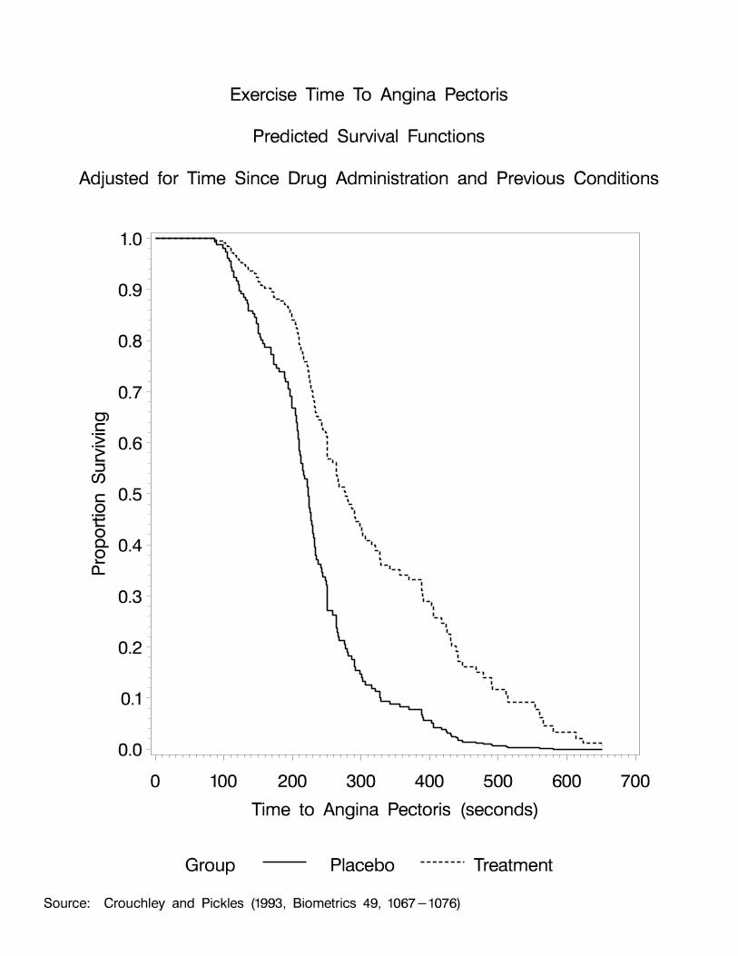

16 SUDAAN Applications
Examples: Data Set 2
Proportional Hazards Model Results
Estimated Regression Estimated Standard Error of BetaCoefficient: Hazards Variance
Treatment vs. Ratio RatioPlacebo
Cluster Independent
-0.8395 0.43 0.1474 0.1724 0.73(27% reduction)
Ü Ü SUDAAN Standard
Packages: Too Large
� True variance (via SUDAAN) smaller than underindependence (e.g., via SAS)
� May fail to detect a treatment effect
yi j
1, Easy
2, Only clear after rereading
3, Not very clear
4, Confusing
Presentation Notes 17
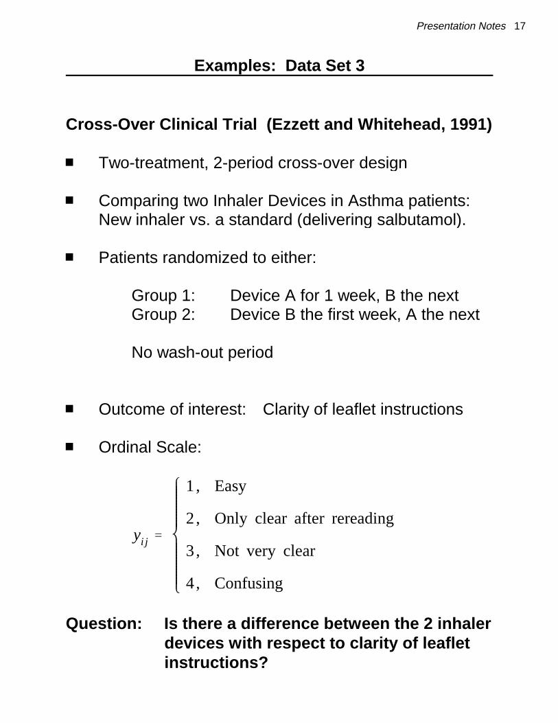
Examples: Data Set 3
Cross-Over Clinical Trial (Ezzett and Whitehead, 1991)
� Two-treatment, 2-period cross-over design
� Comparing two Inhaler Devices in Asthma patients:New inhaler vs. a standard (delivering salbutamol).
� Patients randomized to either:
Group 1: Device A for 1 week, B the nextGroup 2: Device B the first week, A the next
No wash-out period
� Outcome of interest: Clarity of leaflet instructions
� Ordinal Scale:
Question: Is there a difference between the 2 inhalerdevices with respect to clarity of leafletinstructions?

18 SUDAAN Applications
Examples: Data Set 3
Frequency Distribution of Leaflet Clarityin the Cross-Over Clinical Trial
Clarity of Leaflet Instructions
Inhaler Device Total Easy Rereading Not Clear ConfusingRequires
A 286 211 71 2 2
B 286 147 118 15 6
Note: There are 286 patients (clusters) in the study
Source: Ezzet and Whitehead (1991), Statistics in Medicine 10, 901-907.

Presentation Notes 19
Examples: Data Set 3
Proportional Odds Model Results
Estimated Standard Error of BetaRegression VarianceCoefficient: Estimated Ratio
Inhaler A vs. B Odds RatioCluster Independent
1.0137 2.76 0.1566 0.1733 0.78(22% reduction)
Ü Ü SUDAAN Standard
Packages:Too Large
� True variance (via SUDAAN) smaller than underindependence (e.g., via SAS)
� May fail to detect a treatment effect

Predicted Observed
DEFF 1 � 'y (m 1) VCLUSTER
VINDEPENDENCE
20 SUDAAN Applications
Design Effects
� Measures the impact of clustering on variance estimationand statistical inference for a sample statistic (mean,proportion, regression coefficient)
� Proportional to intracluster correlation and cluster size
Means, Proportions :
' = response intracluster correlationy
m = cluster sizeV = variance of the statistic under clustercluster
samplingV = variance of the statistic under independenceindependence
Kish and Frankel (1974)
DEFF = 1: No inflation in variance > 1: Variance inflation (over-dispersion)
' > 0, almost alwaysy

DEFF 1 � 'y 'x (m 1)
Ex: E(y) X�
1, clusterlevel covariates
< 0, withincluster covariates (same patterns)
> 0, withincluster covariates (patterns differ)
Presentation Notes 21
Design Effects
Regression Coefficients:Continuous and Binary Responses*
' = covariate intracluster correlationx
=
Assumes exchangeable correlation structure
Neuhaus and Segal (1993)Scott and Holt (1982) Zeger (1988)
* Proportional hazards survival models:This pattern has been observed in simulation studies, but the exact formula hasnot been developed

'y > 0'x > 0
'y > 0'x < 0
22 SUDAAN Applications
Analysis Implications
DEFF > 1 DEFF < 1
Type I Error Power
Standard Inflated Reduced
SUDAAN Correct Increased
Ü ÜTreatment: Treatment:Cluster-level Within-clustercovariate covariate
e.g., Teratology e.g., Cross-Over Trial

m
'x 1
m 1via Kappa Statistic
DEFF 1 � 'y 'x (m 1)
Presentation Notes 23
How Much Correlation in Typical Studies?
Study Ave. Cluster DesignSize, Effect
' 'y x
Ex 1: 13 .26 1 4.0Teratology
Ex 2: 8 .65 < 0 0.73Angina Exercise TimesCross-Over Study
>
Ex. 3: 2 Matrix of positive -1 0.78Leaflet Clarity and negativeCross-Over Study values
>
>

24 SUDAAN Applications
Design Effects
Relationship to Effective Sample Size
Suppose sample consists of 20 clusters, with 10 observations percluster:
n = 20 clustersm = 10 observations / clusterN = 200 observations in sample (n*m)
'' = Intracluster Correlation Design Effect Sample Sizey
Effective
0 (independence) 1 200 ( = N)
1 (perfect positive correlation) 10 (= m) 20 ( = n)
Design Effect (DEFF) = 1 + ' (m - 1) = V / Vy Cluster Indep
Effective Sample Size (EFF) = N / DEFF
= amount of independentinformation available forcomputing variance of samplestatistics
Usually: 0 < ' < 1 (closer to 0)y
1 < DEFF < 10 (closer to 1)
200 > EFF > 20 (closer to 200, number of obs)

S(t ) Prob(T> t)
h(t ) f (t)S(t )
h(t x ) ho(t ) exp(x ��)
S(t x ) So(t ) exp(x ���)
Presentation Notes 25
Why SUDAAN?A Proportional Hazards Model Simulation Experiment
Survival Function
Hazard Function
Proportional Hazards Model
Variance Estimation
Linearization, combined with a between-cluster varianceestimator:
Binder (1983, International Stat. Review)Binder (1992, Biometrika)Lin and Wei (1989, JASA)Shah, et al (1996). SUDAAN User’s Manual, Rel 7.0Lee, Wei, Amato (1992)Lin (1994, Statistics in Medicine)Williams and Bieler (1993, ASA BiopharmProceedings)

h(t d) h0(t) exp(�d) d0,1,2,3
26 SUDAAN Applications
Why SUDAAN?A Proportional Hazards Model Simulation Experiment
Simulation of a Repeated Measures Study
� Based on the design of a Neurotoxicology Study measuringthe effect of exposure on learning and memory in laboratoryrats
� 4 dose groups
� 25 animals (clusters) per group
� 2 cluster sizes
- 5 measurements per cluster- 20 measurements per cluster
� 2 dose-response relationships
� = 0 No dose response
� = .0951 33% increased hazard in high dose vs.control
� Also analogous to recurrent events observed on samesubject

Presentation Notes 27
Proportional Hazards Simulation Results:Empirical Probabilities of Rejection
H : �� = 00
Intracluster Type I Error PowerCorrelation (Cluster)
Independence Cluster
Cluster Size = 20, Total Sample Size = 2,000
All .00 4.4 4.5 96.8
All .05 12.3 5.0 79.6
All .10 20.1 4.8 64.9
All .20 29.3 5.0 42.0
Cluster Size = 5, Total Sample Size = 500
All .00 5.3 5.9 56.2
All .05 7.0 5.7 46.3
All .10 9.0 5.6 40.5
All .20 11.3 5.1 33.1
Independence: Standard Statistical Packages (e.g., SAS)Cluster: SUDAAN
Type I Error: Two-Tail TestPower: Upper-tail test with true � = 0.0951

28 SUDAAN Applications
Summary of the Proportional Hazards Simulation
� Assuming independence yields inflated Type I errorrates
- Leads to false positive results
- Increases with cluster size
- Increases with intracluster correlation
� SUDAAN methods maintain 5% Type I error for allcluster sizes and levels of intracluster correlation
� SUDAAN gets the variance right
- Average variance estimates for SUDAANmatched the empirical values
H0 : �1 0 vs. H1 : �1 > 0
logp
1 p �0 � �1 D O S E
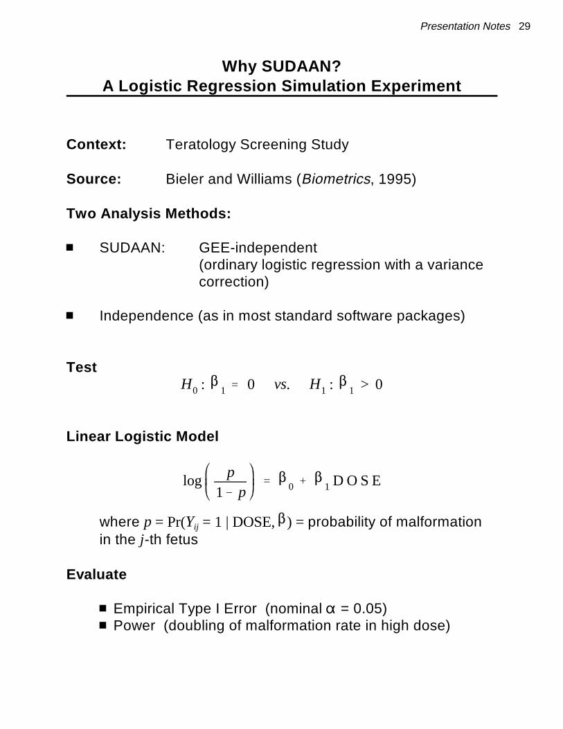
Presentation Notes 29
Why SUDAAN?A Logistic Regression Simulation Experiment
Context: Teratology Screening Study
Source: Bieler and Williams (Biometrics, 1995)
Two Analysis Methods:
� SUDAAN: GEE-independent(ordinary logistic regression with a variancecorrection)
� Independence (as in most standard software packages)
Test
Linear Logistic Model
where p = Pr(Y = 1 | DOSE, �) = probability of malformationij
in the j-th fetus
Evaluate
� Empirical Type I Error (nominal � = 0.05)� Power (doubling of malformation rate in high dose)

30 SUDAAN Applications
Why SUDAAN?A Logistic Regression Simulation Experiment
Design
� Kupper, et al (1986) � Carr (1993)
� 4 dose groups: ln(dosage) = 1,2,3,4 (C, L, M, H) � 25 litters / group � Mean litter size = 11.7 pups
Intralitter Correlations (Beta-binomial model)
� 3 homogeneous
Model
� Linear logistic model � Null Case (background rate = 5%) � Alternative Case (10% in high dose)
Tests
� 1,400 replications � Wald statistic: Z = � / se(�) � Nominal � = .05

Presentation Notes 31
Teratology Simulation Results
Observed Upper-Tail Probabilities of Rejection for the NullHypothesis that the Logistic Slope Parameter = 0
Nominal Alpha = 5%Background Rate = 5%
Test Statistic
Operating High Dose Intralitter SUDAANStandard
Characteristics Rate Correlations Zindep Zcluster
TYPE I ERROR 5% 0 0 0 0 4.0 4.9
5% .1 .1 .1 .1 13.1 4.5
5% .2 .2 .2 .2 17.8 6.9
POWER 10% 0 0 0 0 81.6 84.9
10% .1 .1 .1 .1 69.5 52.0
10% .2 .2 .2 .2 68.9 41.1
Z is the standard Wald test statistic estimated from a linear logisticINDEP
model assuming independence and a binomial likelihood
Z is a Wald test statistic estimated from a linear logistic modelCLUSTER
under a binomial likelihood, with between-cluster variance estimatesbased on Taylor linearization (or: GEE with independent workingcorrelations and a robust variance estimator).

32 SUDAAN Applications
Why SUDAAN?A Logistic Regression Simulation Experiment
Results :
� Assuming independence yields inflated Type I error rates
- Leads to false positive results- Increases with intracluster correlation
� SUDAAN maintained nominal Type I error rates (5%)
� SUDAAN gets the variance right:
- Average variance estimates for SUDAAN matched theempirical values

Presentation Notes 33
Analysis of Clustered Data
Basic Concept
1) Use consistent estimators of the parameters
e.g., Means, Proportions, Percentages, Odds Ratios,Regression Coefficients
� Without imposing strict distributional assumptionsabout the response of interest
� Intracluster correlation treated as a nuisanceparameter
2) Robust variance estimators ensure consistent varianceestimates and valid inferences
Two Variance Estimation Methods in SUDAAN:
� Taylor linearization� Jackknife resampling (new in Release 7.5)

Y
y1
#
#
#
yN
V(Y) )2I N
)2 0 0 á 0
0 )2 0 á 0
0 0 )2 á 0
� � � � �
0 0 0 á )2
Observations independent, constant variance
Y
y11
�
y1m1
�
yn1
�
yn mn
n clusters ofmi observations (N Mn
i1mi )
Unequal observations per cluster mi
Example: n litters with mi pups per litter
34 SUDAAN Applications
Assumptions: Independence Vs. Clustered Data
Independence
Clustered Data (SUDAAN ):

V (Y)
V1 0 0 à 0
0 V2 0 à 0
0 0 V3 à 0
� � � � �
0 0 0 à Vn
ClusterCorrelated Data
BlockDiagonal by Cluster
Vi is an mi x mi matrix
Vi
)2(i)1 )(i)12 )(i)13 à )(i)1 m
)(i)21 )2(i)2 )(i)23 à )(i)2 m
� � �
� � �
)(i)m 1 )(i)m 2 )(i)m 3 à )2(i) m
Vi
Presentation Notes 35
Assumptions: Independence Vs. Clustered Data
Clustered Data (SUDAAN):
� is an m x m variance covariance matrix of observationsi i
in the i-th cluster
� No assumptions on structure of Vi
� Observations independent between clusters, completelyarbitrary correlation structure within clusters

y 1N M
N
i1yi
V ( y) )2
N
1N
MN
i1( yi y )2
N 1
N
N1 MN
i1
yi y
N
2
Zij yij y
NLinearized Value
Zi M
mi
j1Zij Cluster Totals
Z 1n M
n
i1Zi Mean of Cluster Totals
V ( y) n S2
nn 1 M
n
i1(Zi Z)2
36 SUDAAN Applications
Independence Vs. Clustered Data:Estimation of a Mean
Independence
N = number of observations
Between-Unit Variance Estimator
Clustered Data (How is SUDAAN different?)
n = number of clusters
Robust or Between-Cluster Variance Estimator

yij µ � �i � �i j
�i � N(0,)2�) litter effect (cluster)
�i j � N(0,)2�) pup effect
�,� independent
y 1n
1m M
n
i1Mm
j1yij
Var ( y ) )
2�
n�
)2�
n mTrue Variance
E (n S2) )
2�
n�
)2�
n mExpected Value of
BetweenCluster Variance Estimator
Presentation Notes 37
Why Just the Variance of Cluster Totals?
Simple Example (Teratology)
Let
i = 1 , ... , n (n litters)j = 1 , ... , m (m pups per litter)
Then,
This says that the expected value of our between-cluster variance estimator isasymptotically equal to the true variance of the estimated parameter, no matterhow many stages of clustering are present.
It also holds true for unequal sample sizes and more general distributionalassumptions.

p
Mn
i1M
mi
j1yij
Mn
i1mi
Number Malformed FetusesTotal Number of Fetuses
38 SUDAAN Applications
Taylor Linearization Approach:Descriptive Statistics
e.g., Means, Proportions, Odds ratios
Two-Step Procedure for Variance Estimation:
1) Apply Taylor series linearization to approximate functions oflinear statistics (e.g., ratios of random variables)
Example: TeratologyProportion of malformed fetuses in a teratology experiment
Find linear approximation to this nonlinear statistic (Kendall andStuart, 1973);Between-cluster variance formulas available for linear statistics.
Woodruff (1971):� Equivalent computational procedure using Taylor series
linearized values
� Each observational unit gets a linearized value (Z ) for aij
particular statistic.
2) Apply between-cluster variance estimator to the linearizedvalues Zij

F(X ,Y) F(µ X ,µY)
� 0FX µ X(X µ X)
� 0FY µ Y(Y µ Y)
� higher order terms
Var F(X ,Y) ³ E F(X ,Y) F (µ X ,µY) 2
E 0FX µ X(Xµ X) � 0FY µ Y
(Yµ Y) 2
Presentation Notes 39
Taylor Series Expansion
X, Y are two linear statistics
Then,

OR a # db # c
Taylor Series Variance
adbc
2 1a�
1b�
1c�
1d
S(tj ) Nj
i11
di
ri
Greenwood�s Variance Formula
S( tj )2M
j
i1
di
ri (ridi )
Where i denotes death times
40 SUDAAN Applications
Other Examples of Taylor Series Linearization
Odds RatioDisease Not Diseased
Exposed a b
Not Exposed c d
Kaplan-Meier Survival Function
Categorical Data Analysis Grizzle-Starmer-Kochvariance formula forweighted least squares

Presentation Notes 41
Assumptions and Validity for Taylor Approach
� Assume: n clusters selected independently from ahypothetical infinite population of clusters
� No strict distributional assumptions for the response ofinterest ("model-free")
� SUDAAN variance estimator yields consistent estimates ofthe variance as the number of clusters tends to infinity
Method is valid for any underlying intraclustercorrelation structure, as long as:
1) Clusters are statistically independent2) Cluster totals Z can be unbiasedly estimated i
Therefore, specification of an explicit correlationstructure is unnecessary.
� Also valid in presence of additional sources of correlationwithin each clustermate (e.g., multiple levels of nesting)

Y
y1
#
#
#
yN
E(Y ) X �
V (Y ) )2I N
Independent obs, constant variance
b (X �X )1X �Y
Var(b) )2 (X � X )1 )2
V (Y ) )2 I N
42 SUDAAN Applications
Independence Vs. Clustered Data:Fitting Linear Regression Models
Standard Situation: Linear Regression
Standard Solution to Normal Equations :
= Mean Square Error
This variance formula only holds when

V (Y) VY
V1 0 0 à 0
0 V2 0 à 0
0 0 V3 à 0
� � � � �
0 0 0 à Vn
ClusterCorrelated Data
BlockDiagonal by Cluster
Vi is an mi x mi matrix
b (X � X )1 X � Y
Var(b) Vb Estimates each element separately
Vb g )2 (X �X )1 due to clustercorrelated data
Presentation Notes 43
Independence Vs. Clustered Data:Fitting Linear Regression Models
How is SUDAAN different?
Form Taylor series linearized values, Z , for the linear ij
regression coefficients above. Then use between-clustervariance formula to estimate:
KEY POINT:

H0: C�� 0
Q (Cb)� C Var(b) C �� 1 (Cb)
Q (Cb)� )2 C (X ��X )1C �� 1 (Cb)
MSH0
MSerror
� r Fr, N r
Q (Cb)� CVbC �� 1 (Cb)
44 SUDAAN Applications
Independence Vs. Clustered DataFitting Linear Regression Models
Null Hypothesis:
C is a contrast matrix of rank r
General Form for Test Statistic :
Standard Situation
Standard computing formula used by most softwarepackages
SUDAAN Test Statistic :
Does not reduce to any simple computing formula

p
Mn
i1M
mi
j1yij
Mn
i1mi
Presentation Notes 45
Jackknife Variance Estimation
Coming in Release 7.5:Resampling Methods for Correlated Data
Quenouille (1956): Reducing bias in estimationTukey (1958): Approximate confidence intervals
Start With Given Point Estimator:Descriptive statistics (e.g., means, proportions) Regression parameter vectors
Use consistent estimators of location parametersNaively treat the correlated responses as independent
Covariance Estimates for Descriptive Statistics
Binomial proportions (Gladen, 1979 JASA): Proportion of fetuses that are malformed in a teratology study

p(k)
Mn
igkM
mi
j1yij
Mn
igkmi
)2JK
n1n M
n
k1p(k) p(.)
2
p(.)
Mn
k1p(k)
n.
E (yi mi) mi pV (yi mi) h(mi) ,
pp)JK
Y Z � N (0,1)
p
p(.)
46 SUDAAN Applications
Jackknife Variance Estimation
An estimate based on all clusters except the k-th is as follows:
Jackknife Variance Estimate for :
where is the average of the Jackknife estimates:
Assuming
then
µ (�) Mn
i1µ i (�) 0
U(�� ) 0 Log L (�� )0��
MiM
jx�
i j yi j MiM
jx�
i j pi j (�� )
�
µ i (�)
U (�� ) 0
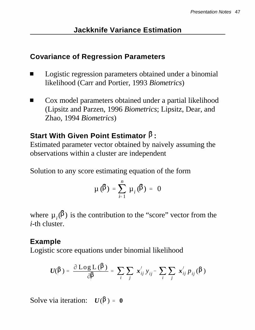
Presentation Notes 47
Jackknife Variance Estimation
Covariance of Regression Parameters
� Logistic regression parameters obtained under a binomiallikelihood (Carr and Portier, 1993 Biometrics)
� Cox model parameters obtained under a partial likelihood(Lipsitz and Parzen, 1996 Biometrics; Lipsitz, Dear, andZhao, 1994 Biometrics)
Start With Given Point Estimator :Estimated parameter vector obtained by naively assuming theobservations within a cluster are independent
Solution to any score estimating equation of the form
where is the contribution to the “score” vector from the i-th cluster.
Example Logistic score equations under binomial likelihood
Solve via iteration:

VarJK (�) np
n Mn
i1�i � �
i ��
�
�
�i
�
48 SUDAAN Applications
Jackknife Variance Estimation
Regression Parameters (continued)
As long as the model for the marginal mean is correctlyspecified, the MLE is asymptotically consistent and normallydistributed
Jackknife Variance Estimator For
where p = number of parameters in the model, and
= estimate of � obtained by deleting the m i
observations in cluster i and solving the estimatingequations via the Newton-Raphson algorithm.
Clusters are removed sequentially and with-replacement
JK variance estimator is consistent for estimating the asymptoticvariance of

Presentation Notes 49
Jackknife Variance Estimation
Regression Parameters (continued)
Simulation in Small Sample SituationsEvaluating treatment effect in logistic regression models (Carrand Portier, Biometrics, 1993)
Jackknife Method:� Controlled Type I error � Estimated location parameters without bias� Estimated variance of parameter estimates without bias� Similar to Zeger/Liang GEE in terms of performance

50 SUDAAN Applications
Assumptions and Validity for Jackknife
� Assume: n clusters selected independently from ahypothetical infinite population of clusters
� No strict distributional assumptions for the response ofinterest
� Jackknife variance estimator yields consistent estimates ofthe variance as the number of clusters tends to infinity
� Method is valid for any underlying intracluster correlationstructure, as long as clusters are statistically independent
� Also valid in presence of additional sources of correlationwithin each clustermate (e.g., multiple levels of nesting)

U(�) Mn
i1
0µ�
i
0�Vi (�)1 (y i µ i ) 0
yi (yi 1, ... ,yimi) Vector of responses
µ i E(yi ) µ i (�� ) Vector of marginal means
(µ i 1 , ... ,µimi)
Vi (��) Cov(yi ; µ i , � ) Working Covariance matrix
Presentation Notes 51
Efficient Parameter Estimation
Efficiently Weight the Data to Estimate RegressionCoefficients ( �)
GEE Approach (Zeger and Liang, 1986):
1) Assume a Covariance Structure for Vi
- Mean / Variance Relationship- Correlation Model
2) Estimate Covariance Parameters
3) Weight Data Inversely Proportional to V to Estimate �i

V i (�) A1/2i R i (��) A1/2
i # 1 V is Block diagonal
A i
g(µ i 1) , ... ,g(µ i mi)
g(µ i 1) 0 0 0
0 g(µ i 2) 0 0
0 0 � �
0 0 à g(µ i mi)
yij
Var(yij ) g(µ i j) # 1
yij
Var(yij ) µ i j (1µ i j ) 1 1
Ri (�) yi
�jk corr (yij , yik )
52 SUDAAN Applications
Covariance Structure for Vi
= diagonal matrix with diagonal elements
=
Relationship Between Variance of and its mean
g is a variance function, 1 is an unknown scale parameter
Binary ResponsesMarginal distribution of is Bernoulli
and .
is the “Working” Correlation Matrix for

Ri (��) I
1 0 0 0
0 1 0 0
0 0 1 0
0 0 0 1
Presentation Notes 53
Choices for Working Correlation Matrices
1) Independent Working Correlation Matrix (Identity matrix)
Form:
� Estimating equations reduce to familiar forms:
- Normal equations for linear regression- Score equations for logistic regression
� Leads to standard regression coefficient estimates
� Consistent and asymptotically normal, even undercluster sampling
� This approach is offered in SUDAAN, and it isperfectly valid for estimating the regressionparameters.

Ri (��)
1 ' ' '
' 1 ' '
' ' 1 '
' ' ' 1
54 SUDAAN Applications
Choices for Working Correlation Matrices
2) Exchangeable(equal pairwise correlations)
Form:
� SUDAAN offers this form as well
� Can improve efficiency of parameter estimates overthe independence working assumption.

Var(�) M 10 M1 M 1
0
where
M0 Mn
i1
0µ�
i
0�V 1
i
0µ i
0�
M1 Mn
i1
0µ�
i
0�V 1
i Var(yi ) V 1i
0µ i
0�
M 10
M1
var (yij ) g g(µ i j ) # 1
Ri (��) Yi
Var(yi ) (yi µ i )(yi µ i )�
Presentation Notes 55
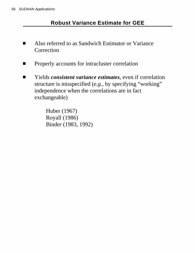
Robust Variance Estimate for GEE
� (outside term) is called the naive or model-based variance(inverse of information matrix, appropriate when covariancestructure correctly specified)
� (middle term) serves as a variance correction when thecovariance model is misspecified
� Robust variance is consistent even when or
is not the true correlation matrix of
� empirically estimated by
� SUDAAN offers the robust and soon (Release 7.5) the model-based variance estimates
56 SUDAAN Applications
Robust Variance Estimate for GEE
� Also referred to as Sandwich Estimator or VarianceCorrection
� Properly accounts for intracluster correlation
� Yields consistent variance estimates, even if correlationstructure is misspecified (e.g., by specifying “working”independence when the correlations are in factexchangeable)
Huber (1967)Royall (1986)Binder (1983, 1992)

E(yij xi j )
Presentation Notes 57
What Does SUDAAN Model?
Marginal Models (Population-Averaged)
� "Marginal mean" of the multivariate outcomes as afunction of the covariates:
� Focus on how X causes Y, while acknowledging thedependence within clusters (as opposed to how one Ycauses another)
� Describes relationship between covariates and responseacross clusters
� Intracluster correlation treated as nuisance parameter
References:
Zeger and Liang (1986)Liang and Zeger (1986)Zeger, Liang, and Albert (1988)Binder (1983, 1992)

58 SUDAAN Applications
SUDAAN Software Package
Software for Statistical Analysis of Correlated Data
� Single program, written in the C language, consisting of afamily of statistical procedures
� As easy to use as SAS!
- Uses a SAS-like interface- Accepts SAS data sets or ASCII files as input
� SPSS Users: Release 7.5 reads SPSS files
� Two Modes of Operation:
1) SAS-Callable (VAX/VMS, IBM/MVS, SUN/Solaris, and soon for Win 95)
2) Stand-Alone (many platforms, including Windows)
� 100% compatible across platforms

Presentation Notes 59
SUDAAN Procedures
DESCRIPTIVE REGRESSIONPROCEDURES PROCEDURES
CROSSTAB REGRESSComputes frequencies, percentage Fits linear regression models anddistributions, odds ratios, relative risks, performs hypothesis tests concerning theand their standard errors (or confidence model parameters. Uses GEE tointervals) for user-specified cross- efficiently estimate regressiontabulations, as well as chi-square tests of parameters, with robust and model-basedindependence and the Cochran-Mantel- variance estimation.Haenszel chi-square test for stratifiedtwo-way tables.
DESCRIPTComputes estimates of means, totals, model parameters; also estimates oddsproportions, percentages, geometric ratios and their 95% confidence intervalsmeans, quantiles, and their standard for each model parameter.errors; also computes standardizedestimates and tests of single degree-of-freedom contrasts among levels of acategorical variable.
RATIOComputes estimates and standard errors and their 95% confidence intervals forof generalized ratios of the form *y / *x, each model parameter; uses GEE towhere x and y are observed variables; efficiently estimate regressionalso computes standardized estimates parameters, with robust and model-basedand tests single-degree-of-freedom variance estimation.contrasts among levels of a categoricalvariable.
LOGISTICFits logistic regression models to binarydata and computes hypothesis tests for
MULTILOGFits multinomial logistic regressionmodels to ordinal and nominal categoricaldata and computes hypothesis tests formodel parameters; estimates odds ratios
SURVIVALFits discrete and continuous proportionalhazards models to failure time data; alsoestimates hazard ratios and their 95%confidence intervals for each modelparameter.
60 SUDAAN Applications
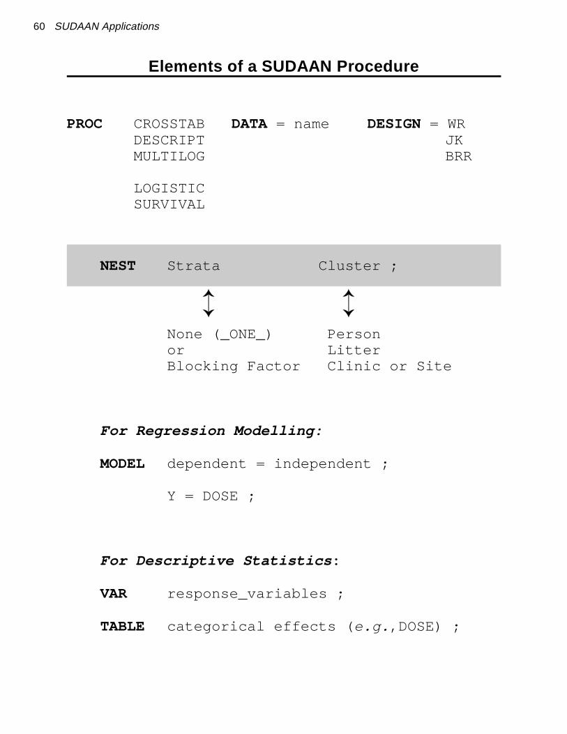
NEST Strata Cluster ;
Elements of a SUDAAN Procedure
PROC CROSSTAB DATA = name DESIGN = WR DESCRIPT JKMULTILOG BRR
LOGISTICSURVIVAL
Ü ÜNone (_ONE_) Personor LitterBlocking Factor Clinic or Site
For Regression Modelling:
MODEL dependent = independent ;
Y = DOSE ;
For Descriptive Statistics :
VAR response_variables ;
TABLE categorical effects ( e.g. ,DOSE) ;

Presentation Notes 61
The MULTILOG Procedure
Multinomial Logistic Regression
� Generalized Logit Models
- Nominal Outcomes
e.g., Type of health plan (A, B, C, D)
� Cumulative Logit Models
- Ordinal Outcomes
e.g., Pain Relief:none, mild, moderate, complete relief
- "Proportional Odds Models"
� Binary Logistic is a special case of each
� Model-fitting Approach
- Fits marginal or population-averagedmodels
- Uses GEE to model the intraclustercorrelations and efficiently estimateregression coefficients

62 SUDAAN Applications
SUDAAN Documentation
Shah, Barnwell, and Bieler (1996). SUDAAN User's Manual, Release7.0, Research Triangle Institute.

Presentation Notes 63
Enhancements to SUDAAN Release 7.5
Resampling Methods for Variance Estimation
� Jackknife� Balanced Repeated Replication (BRR)
Enhancements of GEE Capabilities
� Exchangeable correlations in linear regression (as alreadyin logistic and multinomial logistic in Release 7.0)
� Choice of robust or model-based variances in GEEapplications
Other Regression Enhancements
� REFLEVEL statement to change the reference level forcategorical covariates
� User-friendly contrast statement (the EFFECTS statement)for testing simultaneous regression effects, simple effects ininteraction models, and more
� R-square (Cox and Snell, 1989) in logistic regression� Least Squares Means (LSMEANS) statement in linear
regression
SAS-Callable Platforms
� Windows� SUN/Solaris
Now reads SPSS files (in addition to SAS and ASCII)
64 SUDAAN Applications
References
Applications of SUDAAN and Related TechniquesBieler, G. and Williams, R. (1995). Cluster sampling techniques in quantal response teratology and
developmental toxicity studies. Biometrics 51, 764-776.
Davies, G.M. (1994). Applications of sample survey methodology to repeated measures data structuresin dentistry. Institute of Statistics Mimeo Series No. 2128T. University of North Carolina: Chapel Hill.
Donner, A. (1982). An empirical study of cluster randomization. American Journal of Epidemiology 11,283-286.
Ennett, S.T., Rosenbaum, D.P., Flewelling, R.L., Bieler, G.S., Ringwalt, C.L., and Bailey, S.L. (1994).Long-term evaluation of drug abuse resistance education. Addictive Behaviors, 19, 113-125.
Fung, K.Y., Krewski, D., and Scott, A.J. (1994). Tests for trend in developmental toxicity experimentswith correlated binary data. Risk Analysis 14, 639-648.
Gansky, SA, Koch, GG, and Wilson, J. (1994). Statistical evaluation of relationships between analgesicdose and ordered ratings of pain relief over an eight-hour period. Journal of Biopharmaceutical Statistics4, 233-265.
Graubard, B.I. and Korn, E.L. (1994). Regression analysis with clustered data. Statistics in Medicine13, 509-522.
LaVange, L.M. and Koch, G.G. (1994). Analysis of repeated measures studies with multiple regressionmethods for sample survey data. Presented and the 1994 Drug Information Association Meetings, andsubmitted for publication.
LaVange, L.M., Keyes, L.L., Koch, G.G., and Margolis, P.A. (1994). Application of sample surveymethods for modelling ratios to incidence densities. Statistics in Medicine 13, 343-355.
Norton, E., Bieler, G., Zarkin, G., and Ennett, S. (1996). Analysis of prevention program effectiveness withclustered data using generalized estimating equations. Journal of Consulting and Clinical Psychology 64,919-926.
Rao, J. and Colin, D. (1991). Fitting dose-response models and hypothesis testing in teratologicalstudies. In: Statistics in Toxicology, Krewski and Franklin, eds. NY: Gordon and Breach.
Rao, J. and Scott, A.J. (1992). A simple method for the analysis of clustered binary data. Biometrics 48,577-585.
Schmid, JE, Koch, GG, and LaVange, LE (1991). An overview of statistical issues and methods of meta-analysis. Journal of Biopharmaceutical Statistics, 1, 103-120.
Williams, R.L. (1995). Product-limit survival functions with correlated survival times. Lifetime DataAnalysis 1, 171-186.
Williams, R.L. and Bieler, G.S. (1993). Estimation of proportional hazards models for survival times withnested errors. ASA Proceedings of the Biopharmaceutical Section, 115-120.

References 65
Survey Samplin gBinder, D. (1992). Fitting Cox's proportional hazards models from survey data. Biometrika 79, 139-147.
Binder, D. (1983). On the variances of asymptotically normal estimators from complex surveys.International Statistical Review 51, 279-292.
Cochran, W.G. (1977). Sampling Techniques. Wiley, New York.
Folsom, R.E. (1974). National Assessment Approach to Sampling Error Estimation, Sampling ErrorMonograph. Prepared for the National Assessment of Educational Progress, Denver, CO.
Hansen, M.H., Hurwitz, W.N., and Madow, W.G. (1953). Sample Survey Methods and Theory,Volume I: Methods and Applications. NY: Wiley.
Kendall, M.G. and Stuart, A. (1973). The Advanced Theory of Statistics. NY: Hafner Publishing Co.
Kish, L. (1965). Survey Sampling. NY: Wiley.
Kish, L. and Frankel, M. (1974). Inference from complex samples (with discussion). Journal of the RoyalStatistical Society, Series B, 36, 1-37.
Koch, G.G., Freeman, D.H. and Freeman, J.L. (1975). Strategies in the multivariate analysis of data fromcomplex surveys. International Statistical Review 43, 59-78.
LaVange, L.M., Iannacchione, V.G., and Garfinkel, S. (1986). An application of logistic regressionmethods to survey data: predicting high cost users of medical care. American Statistical Association,Proceedings of the Section on Survey Research Methods, Washington, DC.
Rao, J. And Scott, A. (1987). On simple adjustments to chi-squared tests with sample survey data. Annalsof Statistics, 15, 385-397.
Sarndal, C., Swensson, B., and Wretman, J. (1992). Model-Assisted Survey Sampling. Springer-Verlag,NY.
Scott, A.J. and Holt, D. (1982). The effect of 2-stage sampling on ordinary least squares methods. Journal of the American Statistical Association 77, 848-854.
Shah, B.V., Barnwell, B.G., and Bieler, G.S. (1996). SUDAAN User's Manual, Release 7, First Edition. Research Triangle Institute, RTP, NC.
Shah, B.V. and LaVange, L.M. (1994). Mixed models for survey data. American Statistical Association,Proceedings of the Section on Survey Research Methods.
Shah, B.V., Holt, M.M. and Folsom, R.E. (1977). Inference about regression models from sample surveydata. Bulletin of the International Statistical Institute XLVII, 3, 43-57.
Thomas, D.R. and Rao, J.N.K. (1987). Small-sample comparisons of level and power for simple goodness-of-fit statistics under cluster sampling. JASA 82, 630-636.
Wolter, K.M. (1985). Introduction to Variance Estimation. NY: Springer-Verlag.
Woodruff, R. (1971). A simple method for approximating the variance of a complicated estimate. Journalof the American Statistical Association 66, 411-414.

66 SUDAAN Applications
GEEs and Generalized Linear ModelsCarr, G. and Portier, C. (1993). An evaluation of some methods for fitting dose-response models to
quantal response data. Biometrics 49, 779-791.
Diggle, P., Liang, K.Y., and Zeger, S.L. (1994). Analysis of Longitudinal Data. NY: Oxford UniversityPress.
Dunlop, D.D. (1994). Regression for longitudinal data: a bridge from least squares regression. American Statistician 48, 299-303.
Huber, P.J. (1967). The behavior of maximum likelihood estimates under non-standard conditions. InProceedings of the Fifth Berkeley Symposium on Mathematical Statistics and Probability 1, 221-233.
Karim, M.R. and Zeger, S.L. (1989). GEE: A SAS macro for longitudinal data analysis. TechnicalReport #674 from the Department of Biostatistics, The Johns Hopkins University.
Liang, K. and Zeger, S. (1986). Longitudinal data analysis using generalized linear models. Biometrika73, 13-22.
Lipsitz, S.R., Kim, K. and Zhao, L. (1994a). Analysis of repeated categorical data using generalizedestimating equations. Statistics in Medicine 13, 1149-1163.
Lipsitz, S.R., Fitzmaurice, G.M., Orav, E.J. and Laird, N.M. (1994b). Performance of generalizedestimating equations in practical situations. Biometrics 50, 270-278.
McCullagh, P. and Nelder, J.A. (1989). Generalized Linear Models. NY: Chapman and Hall.
Neuhaus, J.M. and Segal, M.R. (1993). Design effects for binary regression models fitted to dependentdata. Statistics in Medicine 12, 1259-1268.
Prentice, R.L. (1988). Correlated binary regression with covariates specific to each binary observation. Biometrics 44, 1033-1048.
Rotnitzky, A. and Jewell, N.P. (1990). Hypothesis testing of regression parameters in semiparametricgeneralized linear models for cluster correlated data. Biometrika 77, 485-497.
Royall, R.M. (1986). Model robust confidence intervals using maximum likelihood estimators. International Statistical Review 54, 221-226.
Zeger, S. (1988). Commentary. Statistics in Medicine 7, 161-168.
Zeger, S. and Liang, K. (1986). Longitudinal data analysis for discrete and continuous outcomes. Biometrics 42, 121-130.

References 67
Random Effects ModelsBryk, A.S. and Raudenbush, S.W. (1987). Application of hierarchical linear models to assessing change.
Psychological Bulletin, 101, 147-158.
Gibbons, R.D. and Hedeker, D. (1994). Application of random effects probit regression models. Journalof Consulting and Clinical Psychology, 62, 285-296.
Goldstein, H. (1987). Multilevel Models in Educational and Social Research. New York, NY: OxfordUniversity Press.
Hedeker, D.R., Gibbons, R.D., and Flay, B.R. (1994). Random-effects regression models for clustered datawith an example from smoking prevention research. Journal of Consulting and Clinical Psychology, 62,757-765.
Hedeker, D.R., Gibbons, R.D., and Davis, J.M. (1991). Random regression models for multicenter clinicaltrials data. Psychopharmacology Bulletin, 27, 73-77.
Hedeker, D.R. and Gibbons, R.D. (1994). A random-effects ordinal regression model for multilevel analysis. Biometrics 50, 933-944.
Laird, N.M., Donnelly, C., and Ware, J.H. (1992). Longitudinal studies with continuous responses. Statistical Methods in Medical Research 1, 225-247.
Laird, N.M. and Ware, J.H. (1982). Random effects models for longitudinal data. Biometrics 38, 963-974.
Stiratelli, R., Laird, N., and Ware, J.H. (1984). Random-effects model for serial observations with binaryresponses. Biometrics 40, 961-971.
Survival MethodsGreenwood, M. (1926). The natural duration of cancer. Reports on Public Health and Medical Subjects,
33, 1-26.
Lee, E.W., Wei, L.J., and Amato, D.A. (1992). “Cox-type regression analysis for large numbers of smallgroups of correlated failure time observations”. In Klein, J.P. and Goel, P.K. (Eds.), Survival Analysis:State of the Art, Kluwer Academic Publishers, Dordrecht, 237-247.
Lin, D.Y. (1994). Cox regression analysis of multivariate failure time data: the marginal approach. Statistics in Medicine 13, 2233-2246.
Lin, D.Y. and Wei, L.J. (1989). The robust inference for the Cox proportional hazards model. Journal ofthe American Statistical Association, 84, 1074-1078.
Comparisons of GEE and Random Effects ModelsNeuhaus, J.M. (1993). Estimation efficiency and tests of covariate effects with clustered binary data.
Biometrics 49, 989-996.
Neuhaus, J.M., Kalbfleisch, J.D., and Hauck, W.W. (1991). A comparison of cluster-specific andpopulation-averaged approaches for analyzing correlated binary data. International Statistical Review59, 25-35.

68 SUDAAN Applications
Park, T. (1993). A comparison of the generalized estimating equation approach with the maximumlikelihood approach for repeated measurements. Statistics in Medicine 12, 1723-1732.
Zeger, S., Liang, KY, and Albert, P.S. (1988). Models for longitudinal data: a generalized estimatingequation approach. Biometrics 44, 1049-1060.
Jackknife Variance EstimatorsCarr, G. And Portier, C. (1993). An evaluation of some methods for fitting dose-response models to quantal-
response developmental toxicity data. Biometrics 49, 779-791.
Gladen, B. (1979). The use of the jackknife to estimate proportions from toxicological data in the presence oflitter
effects. Journal of the American Statistical Association 74, 278-283.
Lipsitz, S. And Parzen, M. (1996). A jackknife estimator of variance for Cox regression for correlated survivaldata. Biometrics 52, 291-298.
Lipsitz, S., Dear, K., and Zhao, L. (1994). Jackknife estimators of variance for parameter estimates fromestimating equations with applications to clustered survival data. Biometrics 50, 842-846.
Quenouille, M. (1956). Notes on bias in estimation. Biometrika 43, 353-360.
Tukey, J.W. (1958). Bias and confidence in not quite large samples. Annals of Mathematical Statistics, 29, 614.

APPENDIX I
Abstracts of Related Papers

70 SUDAAN Applications

APPENDIX I: Abstracts of Related Papers 71
Statistical Evaluation of Relationships BetweenAnalgesic Dose and Ordered Ratings of Pain Relief
Over an Eight-Hour Period
SA Gansky, GG Koch, and J. Wilson
KEY WORDS: Longitudinal design; relative potency; weighted least squares; ordinal response;multivariate analysis; marginal models.
1994, Journal of Biopharmaceutical Statistics, 4(2), 233-265.
Statistical considerations are discussed for the application of alternative methods to a clinical trialinvolving repeated ordinal ratings and multiple dosage levels of active drugs. Analyses includedsummary measures traditionally employed in studies of acute pain: sum of pain intensity differencesfrom baseline, total pain relief, and total pain half gone. Estimators and confidence intervals of relativepotency are developed for univariate and multivariate situations, using weighted least squares analysiswith mean response and variances from Taylor series linearizations. The estimates from these methodsare compared to those from traditional methods, such as ordinary least squares regression and Fieller'smethod for confidence intervals, as well as those from more recent developments, such as generalizedestimating equations and sample survey data regression. A double-blind, two-center, randomizedclinical trial of acute pain relief comparing placebo with two analgesics, each at two dosage levels, overan 8-hour period serves as an illustrative example for these techniques and comparisons.
An Overview of Statistical Issues andMethods of Meta-Analysis
JE Schmid, GG Koch, and LM LaVange
KEY WORDS: Meta-analysis; random effects model; survey data regression; combination ofstudies
1991, Journal of Biopharmaceutical Statistics, 1(1), 103-120.
A meta-analysis is a statistical analysis of the data from some collection of studies in order to synthesizethe results. In this paper we discuss issues that frequently arise in meta-analysis and give an overview ofthe methods used, with particular attention to the use of fixed- and random-effects approaches. Themethods are then applied to two sample datasets.

72 SUDAAN Applications
CLUSTER SAMPLING TECHNIQUES IN QUANTAL RESPONSETERATOLOGY AND DEVELOPMENTAL TOXICITY STUDIES
Gayle S. Bieler and Rick L. Williams
Contact: Gayle S. Bieler, Research Triangle Institute,P.O. Box 12194, Research Triangle Park, NC 27709
KEY WORDS: clustered binary data; Taylor series variance, dose response; toxicology
This paper presents a model-free approach for evaluating teratology and developmental toxicity datainvolving clustered binary responses. In teratology studies, a major statistical problem arises from theeffect of intralitter correlation, or the potential for littermates to respond similarly. Some statisticalmethods impose strict distributional assumptions to account for extra-binomial variation, while othersrely on nonparametric resampling and empirical variance estimation techniques. Quasi-likelihoodmethods and GEE's, which model the marginal mean/variance relationship, also avoid strictdistributional assumptions. The proposed approach, often used to analyze complex sample survey data,is based on a first-order Taylor series approximation and a between-cluster variance estimationprocedure, yielding consistent variance estimates for binomial-based proportions and regressioncoefficients from dose-response models. The cluster sample technique, presented here in the context ofa logistic dose-response model, incorporates many of the advantages of quasi-likelihood methods, arevalid for any underlying correlation structure, and are adaptable to a variety of analytical settings. Theresults of a simulation study show the cluster sample technique to be a viable competitor to othermethods currently receiving attention.
1995, Biometrics 51, 764-776.
ESTIMATION OF PROPORTIONAL HAZARDS MODELS FORSURVIVAL TIMES WITH NESTED ERRORS
Rick L. Williams and Gayle S. Bieler
KEY WORDS: Correlated failure times; Taylor series variance approximation; Cox regression
A simple variance estimation method is demonstrated for proportional hazards models of survival timeswith a nested error structure. For example, this method is appropriate when repeated measurements aretaken on a single animal in neurobehavioral toxicology experiments, when analyzing littermates interatology studies, or whenever survival times are clustered, as in families or clinics. The methodderives from Binder's (1992) work for complex sample surveys using a Taylor series approach whichyields consistent estimates of the model parameters and their variance-covariance matrix. In asimulation study of the level and power of significance tests of model parameters, we find that themethod maintains the specified Type 1 error rate. We further demonstrate the method using repeatedmeasurements of time to avoidance in a neurobehavioral toxicology experiment. This approach isimplemented in the SUDAAN software package.
1993, American Statistical Association, Proceedings of the Biopharmaceutical Section.

APPENDIX I: Abstracts of Related Papers 73
REGRESSION ANALYSIS WITH CLUSTERED DATA:APPLICATION OF SURVEY METHODOLOGY
B. I. Graubard and E. L. Korn
Contact: B. I. Graubard, National Cancer Institute,6130 Executive Blvd., Bethesda, MD 20892
KEY WORDS: Population average, cluster specific, logistic regression
Clustered data are found in many different types of studies such as repeated measures, inter-rateragreement, household survey, cross-over and community randomized studies. Analyses based onpopulation average (PA) and cluster specific (CS) models are two commonly used approaches forestimating treatment/exposure effects with clustered data. This paper gives conditions involvingmarginal balancing of the covariates and the treatment/exposure variable under which the PA and CSanalyses will agree. A weighted PA analysis is proposed which will estimate CS treatment effects whenmarginal balancing does not hold. Methods for variance estimation which draw upon surveymethodology are proposed for the weighted PA analysis.
1994, Statistics in Medicine 13, 509-522.
APPLICATION OF SAMPLE SURVEY METHODS FOR MODELINGRATIOS TO INCIDENCE DATA
LM LaVange, GG Koch, LL Keyes, and PA Margolis
KEY WORDS: Incidence density analysis, weighted least squares, adverse event associations
We describe ratio estimation methods for analyzing incidence data from follow-up studies. Commonlyused in survey data analysis, these ratio methods require minimal distributional assumptions andaccurately account for random variability in the at-risk periods and correlations among repeated events. The methods are easy to understand, readily available via commercial software, and provide flexibilityfor a variety of analytical settings. We suggest that ratio methods may be useful for epidemiological andclinical studies in which quantities such as incidence of illness events or side effects of drug treatmentare the focus. The basic strategy consists of a two-step process in which we first estimate subgroupspecific incidence densities and their covariance matrix via a first order Taylor series approximation. We then fit log-linear models to the estimated ratios in order to assess covariate effects. The ability toproduce direct estimates of adjusted incidence density ratios is an important advantage of this approach. We provide illustrative analyses of incidence data using ratio methods as well as survey logisticregression methods and two applications of generalized estimating equation methodology, repeatedlogistic and Poisson regression models, for comparison.
1994, Statistics in Medicine 13, 509-522.

74 SUDAAN Applications
APPLICATIONS OF SURVEY SAMPLING METHODOLOGY TOANALYSIS OF REPEATED MEASURES DATA STRUCTURES IN
DENTISTRY
GM Davies and GG Koch
Key Phrases:Intra-patient correlation, Survey data regression, Stratified cluster sample, Dental data
In the dental sciences, researchers often encounter data which are observed at the site or tooth levelwithin each patient. Consequently, statistical methods for repeated measures or clustered outcomes areneeded to analyze dental data with this structure. Survey sampling researchers have developedregression methods to analyze continuous or categorical data from stratified multistage cluster samples. Statistical packages like SUDAAN (Survey Data Analysis) are available to implement such analyses. This paper discusses applications of SUDAAN to a cross-sectional study of school aged children and alongitudinal study of elderly patients over 65. Continuous responses are analyzed with SUDAANprocedures for comparing ratio means and for multiple linear regression; dichotomous responses areanalyzed with SUDAAN procedures for logistic regression. For each application, patients are managedas the primary sampling unit through which adjustment for the correlated data structure within patient isachieved.
1993, Presented at the Biometrics Society Spring Meetings.
ALTERNATIVE METHODS FOR ANALYZING CLUSTERED BINARYDATA IN OPHTHALMOLOGICAL STUDIES
AR Localio, JR Landis, SL Weaver, TJ SharpCenter for Biostatistics and Epidemiology, Penn State University
This paper describes modeling alternatives for binary data in ophthalmology, where clustering(correlation) of eyes within subject is a well-recognized issue, to determine how long after fatal accidentdonor corneas can be transplanted safely. Rabbits were sacrificed, and corneas of one eye wereexamined microscopically to determine the rate of cell death (under 7 per 1,000). Rabbits (andremaining eyes) were either refrigerated or not, and cell death rate was determined at 6 and 24 hours. Modeling the effect of refrigeration and time on cell viability was performed using: (1) logisticregression (LR) (SAS CATMOD) with no consideration of clustering of cells within eye, or thecorrelation of eyes within rabbit, (2) exact LR using LogXact, (3) LR using SUDAAN and consideringthe clustering of cells within eye, (4) LR using SUDAAN and considering two stages of clustering, cellwithin eye and eye within rabbit, (5) GEE with a logistic link and binomial error that accounts forclustering of cells within eye, and (6) cells within rabbit, (7) GEE with log link and Poisson error termthat conditions on eye and accounts for correlation of eyes within rabbit, (8) conditional LR thatconditions on rabbit (STATA), and (9) exact conditional LR (LogXact). Methods are compared both interms of interpretation of parameters and standard errors, and computing requirements for samples of3,000 observations per eye and a total of 130,000 data points.
1993, Presented at the Biometrics Society Spring Meetings.

APPENDIX I: Abstracts of Related Papers 75
ANALYSIS OF REPEATED MEASURES STUDIES WITH MULTIPLEREGRESSION METHODS FOR SAMPLE SURVEY DATA
LM LaVange and GG Koch
This presentation discusses how recently developed statistical procedures for fitting multiple regressionmodels to sample survey data enables more effective analysis for repeated measures studies withcomplicated data structures. Situations where such methods are of interest include dermatology studieswhere treatment is applied to two or more sites of each patient, multi-visit studies where responses areobserved at two or more points for each patient, dental studies where two or more teeth or dental areas ofeach patient receive treatment or are monitored over time for outcomes such as caries or progression ofperiodontal disease, multi-period crossover studies, and epidemiologic studies for repeated occurrencesof adverse events or illnesses. For these situations, one can specify a primary sampling unit withinwhich repeated measures have intraclass correlation. This intraclass correlation is taken into account bysample survey regression methods through robust estimates of the standard errors of the regressioncoefficients. Regression estimates are obtained from model fitting estimation equations which ignorethe correlation structure of the data (i.e., computing procedures which assume that all observational unitsare independent or are from simple random samples). The analytic approach is straightforward to applywith logistic models for dichotomous data, proportional odds models for ordinal data, and linear modelsfor continuously scaled data, and results are interpretable in terms of population average parameters. Several examples are presented to illustrate the capabilities of the methodology.
1994, Presented at the Drug Information Association Annual Meeting.
MIXED MODELS FOR SURVEY DATA
BV Shah and LM LaVange, Research Triangle Institute
Key Words: Mixed models, Maximum Likelihood, Survey Data, Approximate F-test
The classic definition of the likelihood function is limited to simple random samples selected with equalprobability. We propose a generalization of the likelihood function that allows for samples selected withunequal probabilities. With this approach, the problem of analyzing sample survey data with linearmodels is reduced to estimating fixed effects and their variances from a mixed model. In fact, standardmethods for fitting linear models to survey data can be viewed as a MINQUE0 estimation procedure,given a set of assumptions regarding the model for the parent population. This approach has theadvantage of making explicit the assumptions underlying the analysis methods used in current samplesurvey practice. We also explore adjustments to the degrees of freedom for the approximate F-test oftenused in survey data analysis. This approximation can be applied to mixed models in general. Wepresent some simulation results to compare our proposed adjustment to previously recommendedapproximations. The adjusted F statistic allows for the analysis of cases previously thought to beintractable, and also allows for the analysis of survey data under different sets of assumptions, withoutignoring the survey design. Of course, the paper raises many more questions regarding potential modelsand appropriate analysis techniques.
1994, Presented at the Joint Statistical Meetings.

76 SUDAAN Applications
Product-Limit Survival Functions with Correlated Survival Times
Rick L. Williams
Research Triangle Institute
Key Words: Kaplan-Meier estimates, life tables, robust variance, Taylor series linearization,intracluster correlation
A simple variance estimator for product-limit survival functions is demonstrated for survival times withnested errors. Such data arise whenever survival times are observed within clusters of relatedobservations. Greenwood's formula, which assumes independent observations, is not appropriate in thissituation. A robust variance estimator is developed using Taylor series linearized values and thebetween-cluster variance estimator commonly used in multistage sample surveys. A simulation studyshows that the between-cluster variance estimator is approximately unbiased and yields confidenceintervals that maintain the nominal level for several patterns of correlated survival times. The simulationstudy also shows that Greenwood's formula underestimates the variance when the survival times arepositively correlated within a cluster and yields confidence intervals that are too narrow. Extension tolife table methods is also discussed.
1995, Lifetime Data Analysis 1, 171-186.
Analysis of Prevention Program Effectiveness with Clustered Data UsingGeneralized Estimating Equations
E.C. Norton, G.S. Bieler, S.T. Ennett, and G.A. Zarkin
Experimental studies of prevention programs often randomize clusters of individuals rather thanindividuals to treatment conditions. When the correlation among individuals within clusters is notaccounted for in statistical analysis, the standard errors are biased, potentially resulting in misleadingconclusions about the significance of treatment effects. This study demonstrates the GeneralizedEstimating Equation (GEE) method, focusing specifically on the GEE-independent method, to controlfor within-cluster correlation in regression models with either continuous or binary outcomes. The GEE-independent method yields consistent and robust variance estimates. Data from Project DARE, a youthdrug use prevention program, are used for illustration.
1996, Journal of Consulting and Clinical Psychology 74, 278-283.

APPENDIX II
Examples

78 SUDAAN Applications
D E F F 1 � ' (m 1) ,
Example 1: Fetal Death in a Teratology Experiment 79
Teratology Experiment: Clustered Binary Data
Evaluation of the Compound DEHP on Fetal DeathThis example demonstrates the cluster sample or GEE model-fitting techniques (Zeger and Liang, 1986;Liang and Zeger, 1986) and the Jackknife in the context of a typical teratology experiment. Forcomparison, we include results based on a strictly binomial model (independence).
The typical teratology screening experiment involves administration of a compound to pregnant dams ofa given animal species, followed by evaluation of the fetuses just prior to the end of gestation for varioustypes of malformations. The experimental groups consist of a control group and anywhere from 2 to 4exposed groups, representing increasing dosages of the compound under test. The data for this examplehave been taken from Butler (1988) and represent fetal death in CD-1 mice after administration of thecompound DEHP at dosages of 0, 250, 500, 1000, or 1500 ppm during gestation. Sample sizes rangedfrom 24 to 30 litters per group. As reported by Butler, the average litter sizes were slightly larger in thecontrol (13.2) vs. all other dose groups (11.5 to 12.3), but a dose-related trend was not evident for thesedata.
In this example, the observations on fetuses are clustered within litters, and the variance estimationtechniques in SUDAAN are directly applicable for accounting for the intralitter correlation. TheSUDAAN program produces dose-specific descriptive statistics (via PROC DESCRIPT) and fits alogistic dose-response model (via PROC LOGISTIC) based on the teratology experiment. Fordemonstration purposes, we fit two logistic models, one with a single regressor (dose level) and anotherwith indicator variables corresponding to each treatment group.
The sample design option WR (shorthand notation for "with-replacement sampling") on the LOGISTICand DESCRIPT procedure statements invokes the robust variance estimator that is appropriate for theseexperimental data. The NEST statement in SUDAAN indicates that litters (represented by DAM)represent the clusters. The requested test statistics WALDCHI and SATADJCHI refer to the usualWald chi-squared test and the Satterthwaite-adjusted chi-squared test (Rao and Scott, 1987),respectively. The latter test is a modification of the usual Wald statistic and has been shown to havesuperior operating characteristics for multiple-degree-of-freedom hypotheses in small samples (Thomasand Rao, 1987).
The estimated dose group percentages and their standard errors under the cluster sample vs. strictlybinomial models are contained in Figure 1. The incidence of fetal death was lowest in the control, 250ppm, and 500 ppm groups (17%, 10%, and 13%, respectively) and highest in the 1000 ppm and 1500ppm groups (50% and 84%, respectively).
Figure 1 also contains design effects for the binomial-based percentages. The design effect measures theinflation (or deflation) in variance of a sample statistic due to intracluster correlation beyond thatexpected if the data were independent. It is estimated as the ratio of the cluster sample variance obtainedthrough Taylor linearization (V ) vs. independence (V ). The predicted design effect for a meanCluster Indepor proportion is directly proportional to the size of the intracluster correlation and the cluster size (Kishand Frankel, 1974):
where m is the constant cluster size and ' is the intracluster correlation. Neuhaus and Segal (1993)showed that this relationship also provides accurate design effect approximations for coefficients from
m�
MiM
jm 2
ij
MiM
jm ij
,
(VC luster/VIndep)
80 SUDAAN Applications
binary response regression models with exchangeable correlations, a single cluster-level covariate, andvariable cluster sizes. For the case of unequal cluster sizes, it has been recommended that m be replacedby a weighted analogue:
where m is the cluster size for the j-th litter in dose group i. i j
Observed design effects for the dose-specific percentages ranged from 0.85 to 6.32 for
these data (see Figure 1). The 250 and 500 ppm groups had design effects just under 1.0 (when V ³ClusterV ), indicating small but slightly negative intralitter correlations. Using the Pearson correlationIndepcoefficient, Butler reported intracluster correlations of -0.01 in each of these two groups. The controland higher dose groups had correlations closer to 0.3 and 0.4, and we detected substantial design effectsnear 5.0 and above in these groups, indicating greater than a 5-fold increase in the strictly binomialvariance due to intralitter correlation. The observed design effects closely corresponded to the predictedvalues (1) in each group, with predictions based on the dose-specific weighted litter sizes andcorrelations estimated by Butler.
To implement the cluster sample methods (via SUDAAN), we estimated the model parameters under astandard binomial likelihood and computed a robust variance estimate. This is also known as ordinarylogistic regression with a variance correction and is equivalent to a GEE logistic model withindependent “working” correlations (which we refer to as GEE-independent). The Wald chi-square testwas used to evaluate the null hypothesis of no dose-related effect.
For comparison, the same logistic models were also fit using:
1) GEE logistic regression models under exchangeable intralitter correlations (GEE-exchangeable),
2) ordinary logistic regression with Jackknife variance estimation, and 3) ordinary logistic regression with no variance correction.
Results for the GEE and Jackknife approaches were essentially the same. For testing that the slopeparameter from a linear logistic model is equal to zero (Figure 3), the GEE-exchangeable approachyielded a Z-statistic of 9.17, compared to a GEE-independent Z-statistic of 8.63 and a Jackknife Z-statistic of 8.41. The estimated slope parameter was slightly larger using the GEE approach withexchangeable correlations (� = 0.00256 vs. 0.00249 for GEE-independent and Jackknife), but this hadno substantial impact on test statistics. Estimated standard errors for the GEE-exchangeable and GEE-independent approaches were equivalent (0.00029), and for Jackknife the estimated standard error was0.00030. The observed design effect for the logistic model slope parameter was over 5.0 for these data,reflecting substantial intralitter correlations. The impact of this design effect is manifested in an inflatedZ-statistic of 19.76 obtained from ordinary logistic regression with no variance correction.

Example 1: Fetal Death in a Teratology Experiment 81
Structure of the Fetal Death Data
Dose Group Litter ID Fetus ID Y = fetal death1 = Control 0 = alive2 = High Dose 1= dead
1 1 1 0
1 1 2 1
1 1 3 0
1 2 1 0
1 2 2 0
2 10 1 0
2 10 2 1
2 20 1 1
2 20 2 1
2 30 1 1
N = 1,619 records on the file (1,619 fetuses clustered within 131 litters)

Observed DEFFVCLUSTER
VINDEPENDENCE
Predicted DEFF 1 � 'i (mi
�
1)
mi
�
dosespecific weighted litter sizes
(13.62, 12.85, 12.75, 13.14, 12.56)
'i dosespecific intracluster correlation (Butler, 1988)
( 0.30, 0.01, 0.01, 0.42, 0.34)
82 SUDAAN Applications
Figure 1
Descriptive Statistics for Fetal Death in the DEHP Data
Dose Number Number Total Percentage Standard Error Design EffectGroup Litters Fetuses Dead Dead Cluster Indep. Obs. Predicted
Control 30 396 66 16.67 4.11 1.87 4.82 4.79
250 ppm 26 320 32 10.00 1.53 1.68 0.83 0.88
500 ppm 26 319 42 13.17 1.84 1.89 0.95 0.88
1000 ppm 24 276 139 50.36 7.44 3.01 6.10 6.10
1500 ppm 25 308 258 83.77 4.65 2.10 4.89 4.93
Ü Ü SUDAAN Standard
Packages: Too Small
Cluster: SUDAAN (Descript Procedure)Independence: Standard Statistical Packages (e.g., SAS)
Source: Bieler and Williams (1995), Biometrics 51, 764-776.

Example 1: Fetal Death in a Teratology Experiment 83
Figure 2
Logistic Regression for the DEHP Data
Exposed vs. Control Group Contrasts
ContrastModel-FittingMethod � S.E. Z P-Valuei
250 Vs. Control GEE (indep) -0.5878 0.3413 -1.72 0.0874GEE (exch corr) -0.5214 0.3307 -1.58 0.1142Jackknife -0.5878 0.3619 -1.62 0.1068Independence -0.5878 0.2300 -2.56 0.0104
500 Vs. Control GEE (indep) -0.2769 0.3370 -0.82 0.4128GEE (exch corr) -0.2269 0.3310 -0.69 0.4902Jackknife -0.2769 0.3562 -0.78 0.4383Independence -0.2769 0.2135 -1.30 0.1947
1000 Vs. Control GEE (indep) 1.6239 0.4197 3.87 0.0002GEE (exch corr) 1.6938 0.4004 4.23 0.0000Jackknife 1.6239 0.4430 3.67 0.0004Independence 1.6239 0.1808 8.98 0.0000
1500 Vs. Control GEE (indep) 3.2504 0.4523 7.19 0.0000GEE (exch corr) 3.3346 0.4470 7.46 0.0000Jackknife 3.2504 0.4792 6.78 0.0000Independence 3.2504 0.2051 15.85 0.0000
GEE (indep): SUDAAN Logistic ProcedureGEE (exch): SUDAAN Multilog ProcedureJackknife: SUDAAN Logistic Procedure Independence: Standard Packages (e.g., SAS Logistic)

Observed DEFFVGEE Indep.
VINDEPENDENCE
Predicted DEFF 1 � 'y (n�
1)
n�
13.01 for the DEHP data
'y 0.259 for the DEHP data
84 SUDAAN Applications
Figure 3
Logistic Regression for the DEHP Data
Test for Dose-Related Trend ( H : � = 0 )o
Model-Fitting Design EffectMethod S.E. Z P-Value Observed Predicted�
GEE independent 0.00249 0.00029 8.63 0.0000 4.64 4.11
GEE exchangeable 0.00256 0.00029 9.17 0.0000
Jackknife 0.00249 0.00030 8.41 0.0000
Independence 0.00249 0.00013 19.76 0.0000
GEE independent: SUDAAN Logistic ProcedureGEE exchangeable: SUDAAN Multilog ProcedureJackknife: SUDAAN Logistic ProcedureIndependence: Standard Packages (e.g., SAS Logistic)
Source: Bieler and Williams (1995), Biometrics 51, 764-776.

Example 1: Fetal Death in a Teratology Experiment 85
DEAD 1 YesDEAD 0 NoDOSE_5 1 CONTROLDOSE_5 2 250 ppmDOSE_5 3 500 ppmDOSE_5 4 1000 ppmDOSE_5 5 1500 ppmHRS 1 1 hr.HRS 2 3 hrs.HRS 3 5 hrs.HRS 4 Pre-DosingSUDTRT 1 TreatmentSUDTRT 2 Placebo
Figure 4
The LEVEL.DBS File:
Contains Value Labels For SUDAAN Data Examples
Record Layout for the LEVEL.DBS File:
Columns Description1-8 Variable Name9-10 Level of the Variable17-66 Text Label For This Level of the Variable
Note: The LEVEL.DBS file can document multiple datasets in the same directory

86 SUDAAN Applications
Example 1 Results:
Descriptive Statistics
1 PROC DESCRIPT DATA="TERATA" FILETYPE=SAS NOMARG ATLEVEL1=2 DESIGN=WR;
2 NEST _ONE_ DAM;
3 WEIGHT _ONE_;
4 VAR DEAD;
5 CATLEVEL 1;
6 SUBGROUP DOSE_5;
7 LEVELS 5;
8 SETENV LABWIDTH=16 COLWIDTH=10 LINESIZE=78 DECWIDTH=2 PAGESIZE=60;
9 PRINT ATLEV1=" NUMBER LITTERS" NSUM= " NUMBER FETUSES" TOTAL="TOTAL DEAD" PERCENT="PERCENTAGE DEAD" SEPERCENT="STANDARD ERROR" DEFFPCT="DESIGN EFFECT"/ STYLE=NCHS ATLEV1FMT=F7.0 NSUMFMT=F7.0 DEFFPCTFMT=F6.2
SEPERCENTFMT=F8.2 TOTALFMT=F5.0;
10 TITLE "DESCRIPTIVE STATISTICS FOR TERATOLOGY DATA" " " "FETAL DEATH IN CD-1 MICE";
Opened SAS data file C:\TERA\EXAMPLES\TERATA.SSD for reading.
Number of observations read : 1619 Weighted count : 1619 Denominator degrees of freedom : 130

Example 1: Fetal Death in a Teratology Experiment 87
Example 1 Results:
Descriptive Statistics
Date: 03-19-97 Research Triangle Institute Page : 1 Time: 14:53:51 The DESCRIPT Procedure Table : 1
DESCRIPTIVE STATISTICS FOR TERATOLOGY DATA
FETAL DEATH IN CD-1 MICE ----------------------------------------------------------------------------- Variable NUMBER NUMBER TOTAL PERCENTAGE STANDARD DESIGN Dose Group LITTERS FETUSES DEAD DEAD ERROR EFFECT ----------------------------------------------------------------------------- DEAD: Yes CONTROL 30 396 66 16.67 4.11 4.82 250 ppm 26 320 32 10.00 1.53 0.83 500 ppm 26 319 42 13.17 1.84 0.95 1000 ppm 24 276 139 50.36 7.44 6.10 1500 ppm 25 308 258 83.77 4.65 4.89 -----------------------------------------------------------------------------
DESCRIPT used CPU time : 3.74 seconds Elapsed time : 4 seconds Virtual memory : 0.84 MB
These results are contained in Figure 1. Note the NEST statement specification of DAM as theprimary sampling unit (the cluster). With DAM as the cluster and the sample design option WR(with-replacement), the standard errors reported in this table are adjusted for clustering.

88 SUDAAN Applications
Example 1 Results:
Descriptive Statistics
11 PROC DESCRIPT DATA="TERATA" FILETYPE=SAS NOMARG DESIGN=WR;
12 NEST _ONE_ DAM;
13 WEIGHT _ONE_;
14 VAR DEAD;
15 CATLEVEL 1;
16 SUBGROUP DOSE_5;
17 LEVELS 5;
18 CONTRAST DOSE_5 = (-1 1 0 0 0) / NAME = "Low Dose Vs. Control";
19 CONTRAST DOSE_5 = (-1 0 1 0 0) / NAME = "500 ppm Vs. Control";
20 CONTRAST DOSE_5 = (-1 0 0 1 0) / NAME = "1500 ppm Vs. Control";
21 CONTRAST DOSE_5 = (-1 0 0 0 1) / NAME = "High Dose Vs. Control";
22 SETENV LABWIDTH=25 COLWIDTH=10 LINESIZE=78 DECWIDTH=2 PAGESIZE=60;
23 PRINT PERCENT="DIFFERENCE" SEPERCENT="STANDARD ERROR" T_PCT="T-STAT" P_PCT="P-VALUE"/ STYLE=NCHS SEPERCENTFMT=F8.2 T_PCTFMT=F6.2 P_PCTFMT=F7.4;
24 TITLE "DESCRIPTIVE STATISTICS FOR TERATOLOGY DATA" " " "FETAL DEATH IN CD-1 MICE";
Opened SAS data file C:\TERA\EXAMPLES\TERATA.SSD for reading.
Number of observations read : 1619 Weighted count : 1619 Denominator degrees of freedom : 130
Here we construct contrasts to compare the percentages of dead pups across dose groups. We used theCATLEVEL statement to estimate percentages instead of proportions (the response DEAD is a 0-1variable). The design option and NEST statements are equivalent to the previous run. There are 1,619pups on the file and 130 denominator DF (#litters - 1) available for computing variance estimates.

Example 1: Fetal Death in a Teratology Experiment 89
Example 1 Results:
Descriptive Statistics
Date: 03-19-97 Research Triangle Institute Page : 1 Time: 14:53:51 The DESCRIPT Procedure Table : 1
DESCRIPTIVE STATISTICS FOR TERATOLOGY DATA
FETAL DEATH IN CD-1 MICE
Variable = DEAD: Yes. -------------------------------------------------------------------- Contrast STANDARD DIFFERENCE ERROR T-STAT P-VALUE -------------------------------------------------------------------- Low Dose Vs. Control -6.67 4.39 -1.52 0.1310 500 ppm Vs. Control -3.50 4.51 -0.78 0.4386 1500 ppm Vs. Control 33.70 8.50 3.96 0.0001 High Dose Vs. Control 67.10 6.21 10.81 0.0000 --------------------------------------------------------------------
DESCRIPT used CPU time : 4.17 seconds Elapsed time : 5 seconds Virtual memory : 0.92 MB
Here we see that the 1,000 and 1,500 ppm groups have significantly higher fetal death rates than thecontrol group.

90 SUDAAN Applications
Example 1 Results: GEE-Independent Logistic Regression Model
25 PROC LOGISTIC DATA="TERATA" FILETYPE=SAS DESIGN=WR;
26 NEST _ONE_ DAM;
27 WEIGHT _ONE_;
28 SUBGROUP DOSE_5;
29 LEVELS 5;
30 REFLEVEL DOSE_5 = 1;
31 MODEL DEAD = DOSE_5;
32 EFFECTS DOSE_5 = (-1 0 0 0 1) / NAME = "Control vs. High Dose";
33 TEST SATADJCHI WALDCHI;
34 SETENV COLSPCE=1 LABWIDTH=22 COLWIDTH=8 DECWIDTH=4 LINESIZE=78 PAGESIZE=60;
35 PRINT BETA="BETA" SEBETA="S.E." DEFT="DESIGN EFFECT" T_BETA="T:BETA=0" P_BETA="P-VALUE" OR LOWOR UPOR DF="DF" SATADJDF="ADJ DF" WALDCHI=" CHI-SQ (WALD)" SATADCHI=" CHI-SQ (SAT.)" WALDCHP=" P-VALUE (WALD)" SATADCHP=" P-VALUE (SAT.)" /T_BETAFMT=F8.2 DEFTFMT=F6.2 SEBETAFMT=F8.6 ORFMT=F5.2 LOWORFMT=F6.2 UPORFMT=F6.2 DFFMT=F7.0 SATADJDFFMT=F8.2 WALDCHIFMT=F8.2 SATADCHIFMT=F8.2;
36 TITLE "TESTING DOSE GROUP HETEROGENEITY" " " "FETAL DEATH IN CD-1 MICE";
Opened SAS data file C:\TERA\EXAMPLES\TERATA.SSD for reading. Number of zero responses : 1082 Number of non-zero responses : 537
Parameters have converged in 4 iterations
Number of observations read : 1619 Weighted count: 1619 Observations used in the analysis : 1619 Weighted count: 1619 Observations with missing values : 0 Weighted count: 0 Denominator degrees of freedom : 130
Maximum number of estimable parameters for the model is 5 R-Square for dependent variable DEAD (Cox & Snell, 1989): 0.304579
Here we fit a GEE logistic regresion model with independent working correlations. Dose group is modelledas a 5-level categorical covariate so we can compare each group to control. The REFLEVEL statement is used toselect dose group level 1 (control) to be the reference level for DOSE_5 in the model. The R-square statistic isbased on Cox and Snell (1989) as the proportion of the log-likelihood that is explained by the model. TheEFFECTS statement requests a single degree-of-freedom contrast comparing the high dose to control.
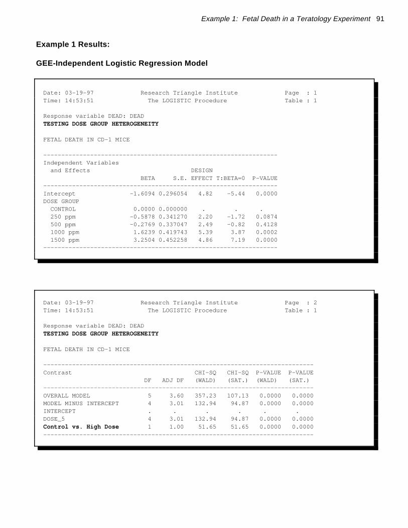
Example 1: Fetal Death in a Teratology Experiment 91
Example 1 Results:
GEE-Independent Logistic Regression Model
Date: 03-19-97 Research Triangle Institute Page : 1 Time: 14:53:51 The LOGISTIC Procedure Table : 1
Response variable DEAD: DEAD TESTING DOSE GROUP HETEROGENEITY
FETAL DEATH IN CD-1 MICE
----------------------------------------------------------------- Independent Variables and Effects DESIGN BETA S.E. EFFECT T:BETA=0 P-VALUE ----------------------------------------------------------------- Intercept -1.6094 0.296054 4.82 -5.44 0.0000 DOSE GROUP CONTROL 0.0000 0.000000 . . . 250 ppm -0.5878 0.341270 2.20 -1.72 0.0874 500 ppm -0.2769 0.337047 2.49 -0.82 0.4128 1000 ppm 1.6239 0.419743 5.39 3.87 0.0002 1500 ppm 3.2504 0.452258 4.86 7.19 0.0000 -----------------------------------------------------------------
Date: 03-19-97 Research Triangle Institute Page : 2 Time: 14:53:51 The LOGISTIC Procedure Table : 1
Response variable DEAD: DEAD TESTING DOSE GROUP HETEROGENEITY
FETAL DEATH IN CD-1 MICE
--------------------------------------------------------------------------- Contrast CHI-SQ CHI-SQ P-VALUE P-VALUE DF ADJ DF (WALD) (SAT.) (WALD) (SAT.) --------------------------------------------------------------------------- OVERALL MODEL 5 3.60 357.23 107.13 0.0000 0.0000 MODEL MINUS INTERCEPT 4 3.01 132.94 94.87 0.0000 0.0000 INTERCEPT . . . . . . DOSE_5 4 3.01 132.94 94.87 0.0000 0.0000 Control vs. High Dose 1 1.00 51.65 51.65 0.0000 0.0000 ---------------------------------------------------------------------------

92 SUDAAN Applications
Example 1 Results:
GEE Independent Logistic Regression Model
Date: 03-19-97 Research Triangle Institute Page : 3 Time: 14:53:51 The LOGISTIC Procedure Table : 1
Response variable DEAD: DEAD TESTING DOSE GROUP HETEROGENEITY
FETAL DEATH IN CD-1 MICE
------------------------------------------ Independent Variables and Effects Lower Upper Odds 95% 95% Ratio Limit Limit ------------------------------------------ Intercept 0.20 0.11 0.36 DOSE GROUP CONTROL 1.00 1.00 1.00 250 ppm 0.56 0.28 1.09 500 ppm 0.76 0.39 1.48 1000 ppm 5.07 2.21 11.63 1500 ppm 25.80 10.55 63.10 ------------------------------------------
LOGISTIC used CPU time : 7.75 seconds Elapsed time : 8 seconds Virtual memory : 1.31 MB
These results indicate that the two highest dose groups have a significantly higher fetal death risk thanthe control group (odds ratios are 5.07 and 25.80, respectively). The treatment effect is statisticallysignificant (p=0.0000).

Example 1: Fetal Death in a Teratology Experiment 93
Example 1 Results:
GEE-Independent Logistic Regression Model
37 PROC LOGISTIC DATA="TERATA" FILETYPE=SAS DESIGN=WR;
38 NEST _ONE_ DAM;
39 WEIGHT _ONE_;
40 MODEL DEAD = DOSE;
41 TEST WALDCHI SATADJCHI; 42 SETENV COLSPCE=1 LABWIDTH=22 COLWIDTH=8 DECWIDTH=4 LINESIZE=78 PAGESIZE=60;
43 PRINT BETA="BETA" SEBETA="S.E." DEFT="DESIGN EFFECT" T_BETA="T:BETA=0" P_BETA="P-VALUE" DF="DF" SATADJDF="ADJ DF" WALDCHI=" CHI-SQ (WALD)" SATADCHI=" CHI-SQ (SAT.)" WALDCHP=" P-VALUE (WALD)" SATADCHP=" P-VALUE (SAT.)" /SEBETAFMT=F8.6 DFFMT=F7.0 T_BETAFMT=F8.2 DEFTFMT=F6.2 SATADJDFFMT=F8.2 WALDCHIFMT=F8.2 SATADCHIFMT=F8.2;
44 TITLE "TESTING DOSE-RELATED TREND" " " "FETAL DEATH IN CD-1 MICE";
Opened SAS data file C:\TERA\EXAMPLES\TERATA.SSD for reading. Number of zero responses : 1082 Number of non-zero responses : 537
Parameters have converged in 4 iterations
Number of observations read : 1619 Weighted count: 1619 Observations used in the analysis : 1619 Weighted count: 1619 Observations with missing values : 0 Weighted count: 0 Denominator degrees of freedom : 130
Maximum number of estimable parameters for the model is 2
R-Square for dependent variable DEAD (Cox & Snell, 1989): 0.277411
Now we model the treatment effect as a continuous covariate, using the actual dosage levels as thecovariate values. For this reason, we do not use a SUBGROUP statement here.

94 SUDAAN Applications
Example 1 Results:
GEE Independent Logistic Regression Model
Date: 03-19-97 Research Triangle Institute Page : 1 Time: 14:53:51 The LOGISTIC Procedure Table : 1
Response variable DEAD: DEAD TESTING DOSE-RELATED TREND
FETAL DEATH IN CD-1 MICE
----------------------------------------------------------------- Independent Variables and Effects DESIGN BETA S.E. EFFECT T:BETA=0 P-VALUE ----------------------------------------------------------------- Intercept -2.4300 0.255035 5.01 -9.53 0.0000 DOSAGE 0.0025 0.000289 5.27 8.63 0.0000 -----------------------------------------------------------------
Date: 03-19-97 Research Triangle Institute Page : 2 Time: 14:53:51 The LOGISTIC Procedure Table : 1
Response variable DEAD: DEAD TESTING DOSE-RELATED TREND
FETAL DEATH IN CD-1 MICE
--------------------------------------------------------------------------- Contrast CHI-SQ CHI-SQ P-VALUE P-VALUE DF ADJ DF (WALD) (SAT.) (WALD) (SAT.) --------------------------------------------------------------------------- OVERALL MODEL 2 1.98 91.65 97.21 0.0000 0.0000 MODEL MINUS INTERCEPT 1 1.00 74.53 74.53 0.0000 0.0000 INTERCEPT 1 1.00 90.78 90.78 0.0000 0.0000 DOSE 1 1.00 74.53 74.53 0.0000 0.0000 ---------------------------------------------------------------------------
LOGISTIC used CPU time : 6.92 seconds Elapsed time : 7 seconds Virtual memory : 1.24 MB
These results indicate there is a significant dose-related trend on the fetal death rate (p=0.0000).

Example 1: Fetal Death in a Teratology Experiment 95
Example 1 Results
Jackknife Variance EstimationBelow are the results obtained using Jackknife variance estimation. The option DESIGN=Jackknife isadded to the PROC statement. All other programming statements are the same as previous. We beginwith dose group modelled as a categorical covariate.
45 PROC LOGISTIC DATA="TERATA" FILETYPE=SAS DESIGN=JACKKNIFE;
46 NEST _ONE_ DAM;
47 WEIGHT _ONE_;
48 SUBGROUP DOSE_5;
49 LEVELS 5;
50 REFLEVEL DOSE_5=1;
51 MODEL DEAD = DOSE_5;
52 EFFECTS DOSE_5 = (-1 0 0 0 1) / NAME = "Control vs. High Dose";
53 TEST SATADJCHI WALDCHI;
54 SETENV COLSPCE=1 LABWIDTH=22 COLWIDTH=8 DECWIDTH=4 LINESIZE=78 PAGESIZE=60;
55 PRINT BETA="BETA" SEBETA="S.E." DEFT="DESIGN EFFECT" T_BETA="T:BETA=0" P_BETA="P-VALUE" OR LOWOR UPOR DF="DF" SATADJDF="ADJ DF" WALDCHI=" CHI-SQ (WALD)" SATADCHI=" CHI-SQ (SAT.)" WALDCHP=" P-VALUE (WALD)" SATADCHP=" P-VALUE (SAT.)" /T_BETAFMT=F8.2 DEFTFMT=F6.2 SEBETAFMT=F8.6 ORFMT=F5.2 LOWORFMT=F6.2 UPORFMT=F6.2 DFFMT=F7.0 SATADJDFFMT=F8.2 WALDCHIFMT=F8.2 SATADCHIFMT=F8.2;
56 TITLE " " "TESTING DOSE GROUP HETEROGENEITY VIA JACKKNIFE" " " "FETAL DEATH IN CD-1 MICE";
Opened SAS data file C:\TERA\EXAMPLES\TERATA.SSD for reading.
Number of observations read : 1619 Weighted count: 1619 Observations used in the analysis : 1619 Weighted count: 1619 Observations with missing values : 0 Weighted count: 0 Denominator degrees of freedom : 130
Maximum number of estimable parameters for the model is 5 Number of zero responses : 1082 Number of non-zero responses : 537
Parameters have converged in 4 iterations
R-Square for dependent variable DEAD (Cox & Snell, 1989): 0.304579

96 SUDAAN Applications
Example 1 Results
Jackknife Variance Estimation
Date: 03-19-97 Research Triangle Institute Page : 1 Time: 14:53:51 The LOGISTIC Procedure Table : 1
Response variable DEAD: DEAD
TESTING DOSE GROUP HETEROGENEITY VIA JACKKNIFE
FETAL DEATH IN CD-1 MICE
----------------------------------------------------------------- Independent Variables and Effects DESIGN BETA S.E. EFFECT T:BETA=0 P-VALUE ----------------------------------------------------------------- Intercept -1.6094 0.314927 5.45 -5.11 0.0000 DOSE GROUP CONTROL 0.0000 0.000000 . . . 250 ppm -0.5878 0.361909 2.48 -1.62 0.1068 500 ppm -0.2769 0.356192 2.78 -0.78 0.4383 1000 ppm 1.6239 0.443029 6.01 3.67 0.0004 1500 ppm 3.2504 0.479198 5.46 6.78 0.0000 -----------------------------------------------------------------
Date: 03-19-97 Research Triangle Institute Page : 2 Time: 14:53:51 The LOGISTIC Procedure Table : 1
Response variable DEAD: DEAD
TESTING DOSE GROUP HETEROGENEITY VIA JACKKNIFE
FETAL DEATH IN CD-1 MICE
--------------------------------------------------------------------------- Contrast CHI-SQ CHI-SQ P-VALUE P-VALUE DF ADJ DF (WALD) (SAT.) (WALD) (SAT.) --------------------------------------------------------------------------- OVERALL MODEL 5 3.59 327.07 96.31 0.0000 0.0000 MODEL MINUS INTERCEPT 4 3.00 119.97 85.19 0.0000 0.0000 INTERCEPT . . . . . . DOSE_5 4 3.00 119.97 85.19 0.0000 0.0000 Control vs. High Dose 1 1.00 46.01 46.01 0.0000 0.0000 ---------------------------------------------------------------------------
Here we see that the estimated regression coefficients for the Jackknife are identical to those used forGEE-independent, but the estimated standard errors are just slightly larger. Nevertheless, the p-valuesfrom the two approaches are still quite similar, and both approaches have been shown to be valid foradjusting for intracluster correlation.

Example 1: Fetal Death in a Teratology Experiment 97
Example 1 Results
Jackknife Variance Estimation
Date: 03-19-97 Research Triangle Institute Page : 3 Time: 14:53:51 The LOGISTIC Procedure Table : 1
Response variable DEAD: DEAD
TESTING DOSE GROUP HETEROGENEITY VIA JACKKNIFE
FETAL DEATH IN CD-1 MICE
------------------------------------------ Independent Variables and Effects Lower Upper Odds 95% 95% Ratio Limit Limit ------------------------------------------ Intercept 0.20 0.11 0.37 DOSE GROUP CONTROL 1.00 1.00 1.00 250 ppm 0.56 0.27 1.14 500 ppm 0.76 0.37 1.53 1000 ppm 5.07 2.11 12.18 1500 ppm 25.80 10.00 66.56 ------------------------------------------
LOGISTIC used CPU time : 19.99 seconds Elapsed time : 20 seconds Virtual memory : 1.25 MB
Since the estimated standard errors are slightly larger for the Jackknife vs. GEE-independent approachesusing these data, the 95% confidence bands around the estimated odds ratios are also slightly widerusing the Jackknife. Note that the odds ratios themselves are identical because the same regressioncoefficients are used for both approaches.

98 SUDAAN Applications
Example 1 Results
Jackknife Variance Estimation
57 PROC LOGISTIC DATA="TERATA" FILETYPE=SAS DESIGN=JACKKNIFE;
58 NEST _ONE_ DAM;
59 WEIGHT _ONE_;
60 MODEL DEAD = DOSE;
61 TEST WALDCHI SATADJCHI;
62 SETENV COLSPCE=1 LABWIDTH=22 COLWIDTH=8 DECWIDTH=4 LINESIZE=78 PAGESIZE=60;
63 PRINT BETA="BETA" SEBETA="S.E." DEFT="DESIGN EFFECT" T_BETA="T:BETA=0" P_BETA="P-VALUE" DF="DF" SATADJDF="ADJ DF" WALDCHI=" CHI-SQ (WALD)" SATADCHI=" CHI-SQ (SAT.)" WALDCHP=" P-VALUE (WALD)" SATADCHP=" P-VALUE (SAT.)" /SEBETAFMT=F8.6 DFFMT=F7.0 T_BETAFMT=F8.2 DEFTFMT=F6.2 SATADJDFFMT=F8.2 WALDCHIFMT=F8.2 SATADCHIFMT=F8.2;
64 TITLE " " "TESTING DOSE-RELATED TREND VIA JACKKNIFE" " " "FETAL DEATH IN CD-1 MICE";
Opened SAS data file C:\TERA\EXAMPLES\TERATA.SSD for reading. Number of observations read : 1619 Weighted count: 1619 Observations used in the analysis : 1619 Weighted count: 1619 Observations with missing values : 0 Weighted count: 0 Denominator degrees of freedom : 130
Maximum number of estimable parameters for the model is 2 Number of zero responses : 1082 Number of non-zero responses : 537
Parameters have converged in 4 iterations
R-Square for dependent variable DEAD (Cox & Snell, 1989): 0.277411
Here are the Jackknife results with dosage modelled as a continuous covariate.

Example 1: Fetal Death in a Teratology Experiment 99
Example 1 Results
Jackknife Variance Estimation
Date: 03-19-97 Research Triangle Institute Page : 1 Time: 14:53:51 The LOGISTIC Procedure Table : 1 Response variable DEAD: DEAD
TESTING DOSE-RELATED TREND VIA JACKKNIFE
FETAL DEATH IN CD-1 MICE
----------------------------------------------------------------- Independent Variables and Effects DESIGN BETA S.E. EFFECT T:BETA=0 P-VALUE ----------------------------------------------------------------- Intercept -2.4300 0.262856 5.32 -9.24 0.0000 DOSAGE 0.0025 0.000297 5.56 8.41 0.0000 -----------------------------------------------------------------
Date: 03-19-97 Research Triangle Institute Page : 2 Time: 14:53:51 The LOGISTIC Procedure Table : 1
Response variable DEAD: DEAD
TESTING DOSE-RELATED TREND VIA JACKKNIFE
FETAL DEATH IN CD-1 MICE
--------------------------------------------------------------------------- Contrast CHI-SQ CHI-SQ P-VALUE P-VALUE DF ADJ DF (WALD) (SAT.) (WALD) (SAT.) --------------------------------------------------------------------------- OVERALL MODEL 2 1.98 86.29 92.58 0.0000 0.0000 MODEL MINUS INTERCEPT 1 1.00 70.66 70.66 0.0000 0.0000 INTERCEPT 1 1.00 85.46 85.46 0.0000 0.0000 DOSE 1 1.00 70.66 70.66 0.0000 0.0000 ---------------------------------------------------------------------------
LOGISTIC used CPU time : 16.92 seconds Elapsed time : 17 seconds Virtual memory : 1.24 MB
These Jackknife results are almost identical to the GEE-independent results shown earlier.

100 SUDAAN Applications

Example 2: Repeated Exercise Times in a Clinical Trial 101
Cross-Over Clinical Trial with Multivariate Failure Time Data:
Evaluation of a Coronary Heart Disease Drug on Repeated Exercise Timesto Angina PectorisThis example demonstrates SUDAAN’s correlated data techniques in the context of a clinical trial. Thedata for this example represent repeated exercise times (in seconds) to angina pectoris in patients withcoronary heart disease. We analyzed the data reported by Crouchley and Pickles (1993), in which 21subjects were each tested four times on one day and a further four times two days later. On each dayexercise time measurements were taken just before and at 1 hour, 3 hours, and 5 hours following drugadministration. On one day the drug was an active treatment (an oral dose of isosorbide dinitrate) and onthe other placebo. Although undertaken as a double-blind randomized cross-over design, the publisheddata do not indicate the order of treatment, preventing any testing for carry-over effects.
The Cox proportional hazards model was used to evaluate the regression effect of treatment (or test day),after adjusting for several covariates: time since drug administration (4-level factor), and indicators forprevious myocardial infarction (MI), previous coronary artery bypass surgery (CAB), and previouspropranolol treatment (PP). Note that treatment day and time since drug administration are within-cluster covariates, while MI, PP, and CAB represent cluster-level covariates. For comparison, weinclude results based on assuming complete independence among the 8 failure times per subject.
The SUDAAN program contains code to fit the Cox proportional hazards model to the observed eventtimes. The default sample design option DESIGN=WR (shorthand notation for "with-replacementsampling") invokes the robust variance estimator that is appropriate for the study. The NEST statementin SUDAAN indicates that the patient (PATIENT) represents the cluster or primary sampling unit, withthe keyword _ONE_ indicating there is a single design stratum. Additional sources of intraclustercorrelation, such as time within each study day, need not be specified. The requested test statisticsWALDCHI and SATADJCHI refer to the usual Wald chi-square test and the Satterthwaite-adjusted chi-square test (Rao and Scott, 1987), respectively. The latter test is a modification of the usual Waldstatistic and has been shown to have superior operating characteristics for multiple-degree-of-freedomhypotheses in small samples (Thomas and Rao, 1987).
Three sets of proportional hazards models were fit:
1) Model 1 was the main effects model, and it included the main effects of treatment (orstudy day), time since drug administration (modelled as a 4-level categorical variablecorresponding to pre-dosing, 1-hour, 3-hours, and 5-hours post-dosing), and the threecontinuous covariates MI, CAB, and PP.
2) Model 2 was the interaction model, containing the main effects in Model 1 and theinteraction effects between treatment and time since drug administration.
3) Finally, in Model 3 we evaluated the simple effects of treatment at each of the four timessince drug administration. Model 3 required four separate runs of the proportionalhazards model containing the treatment effect and the three continuous covariates. Thefour runs corresponded to each of the four times since drug administration.
SUDAAN results from fitting Models 1-3 are contained in the SUDAAN output, and results from the

102 SUDAAN Applications
main effects model are contained in Figure 1.
To implement the cluster sample methods using SUDAAN, we estimated the model parameters under astandard partial likelihood and applied a robust variance estimator (labelled Robust in Figure 1). TheWald chi-square test was used to evaluate the null hypothesis of no treatment effect. For comparison,the same proportional hazards model was also fit assuming complete independence of the response times(labelled Naive in Figure 1).
Figure 1 contains results for the main effects model. Note that for parameters which represent cluster-level covariates, the cluster sample method results in a substantial increase in standard errors. However,for within-cluster covariates (e.g., the treatment and time effects), the cluster variance estimates aresubstantially smaller than the independence estimates. Using the design effect results of Neuhaus andSegal (1993) and proceeding by analogy to failure time data, the large observed design effects for thecluster-level covariates (e.g., previous bypass surgery) indicate large response intracluster correlations. In this situation, the variance of the regression coefficients for such covariates is increased. However,the observed design effects for within-cluster covariates whose patterns do not vary from cluster tocluster (time since drug administration and treatment day) were much less than 1 (as low as 0.30), whichwould be expected when the response intracluster correlation is positive and the covariate intraclustercorrelation is negative. In this case, variance estimates for the regression coefficients would be smallerthan that expected under independence, corresponding to a gain in efficiency.
As seen in Figure 1, tests for treatment effects and time since drug administration were statisticallysignificant under the cluster sample and independence approaches, but were slightly more significantunder the cluster sample approach. Using cluster sample techniques, SUDAAN reports the estimatedhazard ratio for treatment vs. control in the main effects only model to be 0.43, with a 95% confidenceinterval of (0.32 - 0.59). A hazard ratio less than 1.0 indicates longer exercise times in the treatmentgroup (a protective effect against angina pectoris), and this can be seen in the predicted survival (Kaplan-Meier) functions (computed at pre-dosing, and 1-, 3-, and 5-hours post-dosing). The Kaplan-Meierfunctions suggest that the treatment differences are largest at 1 and 3-hours post-dosing, and in fact,SUDAAN reports a significant interaction effect between treatment day and time since drugadministration (p=0.0204, Wald chi-square test). The estimated hazard ratios at 1 and 3-hours post-dosing are 0.28 and 0.34, respectively; and the hazard ratios at pre-dosing and 5-hours post-dosing are0.56 and 0.48, respectively.
Tests for the cluster-level covariates (previous MI, bypass surgery, and propranolol treatment) becameless significant under the cluster sample approach, and only previous myocardial infarction remainedstatistically significant in each of the three models (interaction, main effects, and time-specific treatmenteffects models) due to the large design effects. A user-defined general linear contrast for testing the jointeffects of the three covariates is demonstrated for the main effects model (via the EFFECTS statement).

Example 2: Repeated Exercise Times in a Clinical Trial 103
Cross-Over Clinical Trial
Repeated Exercise Times to Angina Pectoris (Crouchley and Pickles, Biometrics, 1993)
� Double-blind randomized cross-over design(not enough info to test carry-over effects)
� 21 male patients (clusters) with coronary heart disease
� Tested 4 times on each of two consecutive days(Cluster size = 8)
Just before drug administration1 hr post3 hrs post5 hrs post
� One day: Active treatment (isosorbide dinitrate)Other day: Placebo
� Outcome at each of 8 time points:
y = exercise time to angina pectoris (in seconds)
Question: Does treatment delay the time to angina pectoris,after adjusting for time since drug administrationand previous conditions?

104 SUDAAN Applications
Structure of the Angina Data
Patient ID Treatment Day Drug Admin Exercise Time MITime Since Y =
(Hours) (seconds)
1 1 = Placebo Day 1 = Pre 150 1
1 1 2 = 1 hr 172 1
1 1 3 = 3 hrs 118 1
1 1 4 = 5 hrs 143 1
1 2 = Treatment Day 1 136 1
1 2 2 445 1
1 2 3 393 1
1 2 4 226 1
2 1 = Placebo Day 1 205 0
2 1 2 287 0
2 1 3 211 0
2 1 4 207 0
2 2 = Treatment Day 1 250 0
2 2 2 306 0
2 2 3 206 0
2 2 4 224 0
N = 168 records (21 patients, 8 records per patient)
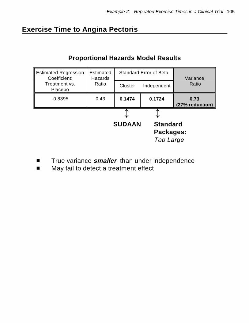
Example 2: Repeated Exercise Times in a Clinical Trial 105
Exercise Time to Angina Pectoris
Proportional Hazards Model Results
Estimated Regression Estimated Standard Error of BetaCoefficient: Hazards Variance
Treatment vs. Ratio RatioPlacebo
Cluster Independent
-0.8395 0.43 0.1474 0.1724 0.73(27% reduction)
Ü Ü SUDAAN Standard
Packages: Too Large
� True variance smaller than under independence� May fail to detect a treatment effect
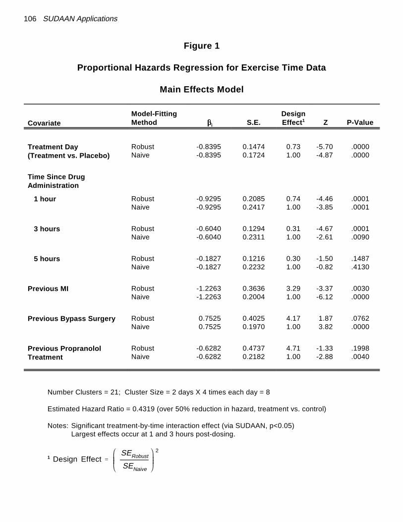
Design Effect SERobust
SENaive
2
106 SUDAAN Applications
Figure 1
Proportional Hazards Regression for Exercise Time Data
Main Effects Model
CovariateModel-Fitting DesignMethod �� S.E. Effect Z P-Valuei
1
Treatment Day(Treatment vs. Placebo)
Robust -0.8395 0.1474 0.73 -5.70 .0000Naive -0.8395 0.1724 1.00 -4.87 .0000
Time Since DrugAdministration
1 hour Robust -0.9295 0.2085 0.74 -4.46 .0001Naive -0.9295 0.2417 1.00 -3.85 .0001
3 hours Robust -0.6040 0.1294 0.31 -4.67 .0001Naive -0.6040 0.2311 1.00 -2.61 .0090
5 hours Robust -0.1827 0.1216 0.30 -1.50 .1487Naive -0.1827 0.2232 1.00 -0.82 .4130
Previous MI Robust -1.2263 0.3636 3.29 -3.37 .0030Naive -1.2263 0.2004 1.00 -6.12 .0000
Previous Bypass Surgery Robust 0.7525 0.4025 4.17 1.87 .0762Naive 0.7525 0.1970 1.00 3.82 .0000
Previous PropranololTreatment
Robust -0.6282 0.4737 4.71 -1.33 .1998Naive -0.6282 0.2182 1.00 -2.88 .0040
Number Clusters = 21; Cluster Size = 2 days X 4 times each day = 8
Estimated Hazard Ratio = 0.4319 (over 50% reduction in hazard, treatment vs. control)
Notes: Significant treatment-by-time interaction effect (via SUDAAN, p<0.05)Largest effects occur at 1 and 3 hours post-dosing.
1

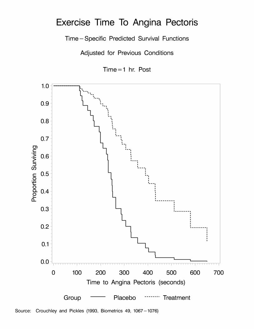


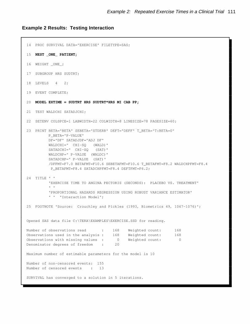
Example 2: Repeated Exercise Times in a Clinical Trial 111
Example 2 Results: Testing Interaction
14 PROC SURVIVAL DATA="EXERCISE" FILETYPE=SAS;
15 NEST _ONE_ PATIENT;
16 WEIGHT _ONE_;
17 SUBGROUP HRS SUDTRT;
18 LEVELS 4 2;
19 EVENT COMPLETE;
20 MODEL EXTIME = SUDTRT HRS SUDTRT*HRS MI CAB PP;
21 TEST WALDCHI SATADJCHI;
22 SETENV COLSPCE=1 LABWIDTH=22 COLWIDTH=8 LINESIZE=78 PAGESIZE=60;
23 PRINT BETA="BETA" SEBETA="STDERR" DEFT="DEFF" T_BETA="T:BETA=0" P_BETA="P-VALUE" DF="DF" SATADJDF="ADJ DF" WALDCHI=" CHI-SQ (WALD)" SATADCHI=" CHI-SQ (SAT)" WALDCHP=" P-VALUE (WALDC)" SATADCHP=" P-VALUE (SAT)" /DFFMT=F7.0 BETAFMT=F10.6 SEBETAFMT=F10.6 T_BETAFMT=F8.2 WALDCHPFMT=F8.4 P_BETAFMT=F8.4 SATADCHPFMT=F8.4 DEFTFMT=F6.2;
24 TITLE " " "EXERCISE TIME TO ANGINA PECTORIS (SECONDS): PLACEBO VS. TREATMENT" " " "PROPORTIONAL HAZARDS REGRESSION USING ROBUST VARIANCE ESTIMATOR" " " "Interaction Model";
25 FOOTNOTE "Source: Crouchley and Pickles (1993, Biometrics 49, 1067-1076)";
Opened SAS data file C:\TERA\EXAMPLES\EXERCISE.SSD for reading.
Number of observations read : 168 Weighted count: 168 Observations used in the analysis : 168 Weighted count: 168 Observations with missing values : 0 Weighted count: 0 Denominator degrees of freedom : 20
Maximum number of estimable parameters for the model is 10
Number of non-censored events: 155 Number of censored events : 13
SURVIVAL has converged to a solution in 5 iterations.

112 SUDAAN Applications
Example 2 Results: Testing Interaction
Date: 03-24-97 Research Triangle Institute Page : 1 Time: 08:50:19 The SURVIVAL Procedure Table : 1
For response variable EXTIME: Exercise Time to Angina Pectoris
EXERCISE TIME TO ANGINA PECTORIS (SECONDS): PLACEBO VS. TREATMENT
PROPORTIONAL HAZARDS REGRESSION USING ROBUST VARIANCE ESTIMATOR
Interaction Model
----------------------------------------------------------------------- Independent Variables and Effects BETA STDERR DEFF T:BETA=0 P-VALUE ----------------------------------------------------------------------- Day Treatment -0.405588 0.133014 0.18 -3.05 0.0063 Placebo 0.000000 0.000000 . . . Hours Since Drug Admin 1 hr. -0.463372 0.201299 0.42 -2.30 0.0322 3 hrs. -0.339857 0.132493 0.18 -2.57 0.0185 5 hrs. -0.087686 0.113670 0.13 -0.77 0.4495 Pre-Dosing 0.000000 0.000000 . . . Day, Hours Since Drug Admin Treatment, 1 hr. -1.107631 0.413010 0.72 -2.68 0.0143 Treatment, 3 hrs. -0.639324 0.251528 0.30 -2.54 0.0194 Treatment, 5 hrs. -0.228561 0.195745 0.19 -1.17 0.2567 Treatment, Pre-Dosing 0.000000 0.000000 . . . Placebo, 1 hr. 0.000000 0.000000 . . . Placebo, 3 hrs. 0.000000 0.000000 . . . Placebo, 5 hrs. 0.000000 0.000000 . . . Placebo, Pre-Dosing 0.000000 0.000000 . . . Previous MI -1.239716 0.370078 3.38 -3.35 0.0032 Previous Bypass Surgery 0.736154 0.403746 4.18 1.82 0.0832 Previous Propranolol Trt -0.615225 0.484650 4.91 -1.27 0.2189 ----------------------------------------------------------------------- Source: Crouchley and Pickles (1993, Biometrics 49, 1067-1076)

Example 2: Repeated Exercise Times in a Clinical Trial 113
Example 2 Results: Testing Interaction
Date: 03-24-97 Research Triangle Institute Page : 2 Time: 08:50:19 The SURVIVAL Procedure Table : 1
For response variable EXTIME: Exercise Time to Angina Pectoris
EXERCISE TIME TO ANGINA PECTORIS (SECONDS): PLACEBO VS. TREATMENT
PROPORTIONAL HAZARDS REGRESSION USING ROBUST VARIANCE ESTIMATOR
Interaction Model
--------------------------------------------------------------------------- CHI-SQ CHI-SQ P-VALUE P-VALUE Contrast DF ADJ DF (WALD) (SAT) (WALDC) (SAT) --------------------------------------------------------------------------- OVERALL MODEL 10 3.98 44.84 20.81 0.0000 0.0004 SUDTRT . . . . . . HRS . . . . . . SUDTRT * HRS 3 1.80 9.80 10.35 0.0204 0.0046 MI 1 1.00 11.22 11.22 0.0008 0.0008 CAB 1 1.00 3.32 3.32 0.0683 0.0686 PP 1 1.00 1.61 1.61 0.2043 0.2046 --------------------------------------------------------------------------- Source: Crouchley and Pickles (1993, Biometrics 49, 1067-1076)
SURVIVAL used CPU time : 3.29 seconds Elapsed time : 4 seconds Virtual memory : 1.08 MB

114 SUDAAN Applications
Example 2 Results: Testing Main Effects
1 PROC SURVIVAL DATA="EXERCISE" FILETYPE=SAS;
2 NEST _ONE_ PATIENT;
3 WEIGHT _ONE_;
4 SUBGROUP HRS SUDTRT;
5 LEVELS 4 2;
6 EVENT COMPLETE;
7 MODEL EXTIME = SUDTRT HRS MI CAB PP;
8 EFFECTS MI CAB PP / NAME = "Combined Effect: MI,CAB,PP";
9 TEST WALDCHI SATADJCHI;
10 SETENV COLSPCE=1 LABWIDTH=22 COLWIDTH=8 LINESIZE=78 PAGESIZE=60;
11 PRINT BETA="BETA" SEBETA="STDERR" DEFT="DEFF" T_BETA="T:BETA=0" P_BETA="P-VALUE" HR LOWHR UPHR DF="DF" SATADJDF="ADJ DF" WALDCHI=" CHI-SQ (WALD)" SATADCHI=" CHI-SQ (SAT)" WALDCHP=" P-VALUE (WALDC)" SATADCHP=" P-VALUE (SAT)" /DFFMT=F7.0 BETAFMT=F10.6 SEBETAFMT=F10.6 T_BETAFMT=F8.2 WALDCHPFMT=F8.4 P_BETAFMT=F8.4 SATADCHPFMT=F8.4 DEFTFMT=F6.2 HRFMT=F7.2 LOWHRFMT=F6.2 UPHRFMT=F6.2;
12 TITLE " " "EXERCISE TIME TO ANGINA PECTORIS (SECONDS): PLACEBO VS. TREATMENT" " " "PROPORTIONAL HAZARDS REGRESSION USING ROBUST VARIANCE ESTIMATOR:" " " "Main Effects Model";
13 FOOTNOTE "Source: Crouchley and Pickles (1993, Biometrics 49, 1067-1076)";
NOTE: Terms in the MODEL statement have been rearranged to follow subgroup order.
Opened SAS data file C:\TERA\EXAMPLES\EXERCISE.SSD for reading.
Number of observations read : 168 Weighted count: 168 Observations used in the analysis : 168 Weighted count: 168 Observations with missing values : 0 Weighted count: 0 Denominator degrees of freedom : 20
Maximum number of estimable parameters for the model is 7
Number of non-censored events: 155 Number of censored events : 13 SURVIVAL has converged to a solution in 5 iterations.

Example 2: Repeated Exercise Times in a Clinical Trial 115
Example 2 Results: Testing Main Effects
Date: 03-24-97 Research Triangle Institute Page : 1 Time: 08:50:19 The SURVIVAL Procedure Table : 1
For response variable EXTIME: Exercise Time to Angina Pectoris
EXERCISE TIME TO ANGINA PECTORIS (SECONDS): PLACEBO VS. TREATMENT
PROPORTIONAL HAZARDS REGRESSION USING ROBUST VARIANCE ESTIMATOR:
Main Effects Model
----------------------------------------------------------------------- Independent Variables and Effects BETA STDERR DEFF T:BETA=0 P-VALUE ----------------------------------------------------------------------- Hours Since Drug Admin 1 hr. -0.929513 0.208504 0.74 -4.46 0.0002 3 hrs. -0.603992 0.129440 0.31 -4.67 0.0001 5 hrs. -0.182658 0.121615 0.30 -1.50 0.1487 Pre-Dosing 0.000000 0.000000 . . . Day Treatment -0.839508 0.147408 0.73 -5.70 0.0000 Placebo 0.000000 0.000000 . . . Previous MI -1.226269 0.363640 3.29 -3.37 0.0030 Previous Bypass Surgery 0.752530 0.402488 4.17 1.87 0.0762 Previous Propranolol Trt -0.628185 0.473715 4.71 -1.33 0.1998 ----------------------------------------------------------------------- Source: Crouchley and Pickles (1993, Biometrics 49, 1067-1076)

116 SUDAAN Applications
Example 2 Results: Testing Main Effects (continued)
Date: 03-24-97 Research Triangle Institute Page : 2 Time: 08:50:19 The SURVIVAL Procedure Table : 1
For response variable EXTIME: Exercise Time to Angina Pectoris
EXERCISE TIME TO ANGINA PECTORIS (SECONDS): PLACEBO VS. TREATMENT
PROPORTIONAL HAZARDS REGRESSION USING ROBUST VARIANCE ESTIMATOR:
Main Effects Model
--------------------------------------------------------------------------- CHI-SQ CHI-SQ P-VALUE P-VALUE Contrast DF ADJ DF (WALD) (SAT) (WALDC) (SAT) --------------------------------------------------------------------------- OVERALL MODEL 7 3.57 49.58 20.57 0.0000 0.0003 HRS 3 2.29 31.22 30.73 0.0000 0.0000 SUDTRT 1 1.00 32.43 32.43 0.0000 0.0000 MI 1 1.00 11.37 11.37 0.0007 0.0008 CAB 1 1.00 3.50 3.50 0.0615 0.0618 PP 1 1.00 1.76 1.76 0.1848 0.1851 Combined Effect: MI,CAB,PP 3 2.86 15.43 13.17 0.0015 0.0039 --------------------------------------------------------------------------- Source: Crouchley and Pickles (1993, Biometrics 49, 1067-1076)

Example 2: Repeated Exercise Times in a Clinical Trial 117
Example 2 Results: Testing Main Effects (continued)
Date: 03-24-97 Research Triangle Institute Page : 3 Time: 08:50:19 The SURVIVAL Procedure Table : 1
For response variable EXTIME: Exercise Time to Angina Pectoris
EXERCISE TIME TO ANGINA PECTORIS (SECONDS): PLACEBO VS. TREATMENT
PROPORTIONAL HAZARDS REGRESSION USING ROBUST VARIANCE ESTIMATOR:
Main Effects Model
------------------------------------------------ Lower Upper Independent Variables Hazards 95% 95% and Effects Ratio Limit Limit ------------------------------------------------ Hours Since Drug Admin 1 hr. 0.39 0.26 0.61 3 hrs. 0.55 0.42 0.72 5 hrs. 0.83 0.65 1.07 Pre-Dosing 1.00 1.00 1.00 Day Treatment 0.43 0.32 0.59 Placebo 1.00 1.00 1.00 Previous MI 0.29 0.14 0.63 Previous Bypass Surgery 2.12 0.92 4.91 Previous Propranolol Trt 0.53 0.20 1.43 ------------------------------------------------ Source: Crouchley and Pickles (1993, Biometrics 49, 1067-1076)
SURVIVAL used CPU time : 3.0 seconds Elapsed time : 3 seconds Virtual memory : 1.08 MB

118 SUDAAN Applications
Example 2 Results: Pre-Dosing Treatment Effect
26 PROC SURVIVAL DATA="EXERCISE" FILETYPE=SAS;
27 NEST _ONE_ PATIENT;
28 WEIGHT _ONE_;
29 SUBPOPN HOURS=1 / NAME = "PRE-DOSING TREATMENT EFFECT";
30 SUBGROUP SUDTRT;
31 LEVELS 2;
32 EVENT COMPLETE;
33 MODEL EXTIME = SUDTRT MI CAB PP;
34 TEST WALDCHI SATADJCHI;
35 SETENV COLSPCE=1 LABWIDTH=22 COLWIDTH=8 LINESIZE=78 PAGESIZE=60;
36 PRINT BETA="BETA" SEBETA="STDERR" DEFT="DEFF" T_BETA="T:BETA=0" P_BETA="P-VALUE" HR LOWHR UPHR DF="DF" SATADJDF="ADJ DF" WALDCHI=" CHI-SQ (WALD)" SATADCHI=" CHI-SQ (SAT)" WALDCHP=" P-VALUE (WALDC)" SATADCHP=" P-VALUE (SAT)" /DFFMT=F7.0 BETAFMT=F10.6 SEBETAFMT=F10.6 T_BETAFMT=F8.2 WALDCHPFMT=F8.4 P_BETAFMT=F8.4 SATADCHPFMT=F8.4 DEFTFMT=F6.2 HRFMT=F7.2 LOWHRFMT=F7.2 UPHRFMT=F7.2;
37 TITLE " " "EXERCISE TIME TO ANGINA PECTORIS (SECONDS): PLACEBO VS. TREATMENT" " " "PROPORTIONAL HAZARDS REGRESSION USING CLUSTER SAMPLE TECHNIQUE" " ";
38 FOOTNOTE "Source: Crouchley and Pickles (1993, Biometrics 49, 1067-1076)";
Opened SAS data file C:\TERA\EXAMPLES\EXERCISE.SSD for reading.
Number of observations read : 168 Weighted count: 168 Observations in subpopulation : 42 Weighted count: 42 Observations used in the analysis : 42 Weighted count: 42 Observations with missing values : 0 Weighted count: 0 Denominator degrees of freedom : 20
Maximum number of estimable parameters for the model is 4
Number of non-censored events: 42 Number of censored events : 0 WARNING: All values of the censoring variable COMPLETE are 1. SURVIVAL has converged to a solution in 5 iterations.

Example 2: Repeated Exercise Times in a Clinical Trial 119
Example 2 Results: Pre-Dosing Treatment Effect
Date: 03-24-97 Research Triangle Institute Page : 1 Time: 08:50:19 The SURVIVAL Procedure Table : 1
For response variable EXTIME: Exercise Time to Angina Pectoris For Subpopulation: PRE-DOSING TREATMENT EFFECT
EXERCISE TIME TO ANGINA PECTORIS (SECONDS): PLACEBO VS. TREATMENT
PROPORTIONAL HAZARDS REGRESSION USING CLUSTER SAMPLE TECHNIQUE
----------------------------------------------------------------------- Independent Variables and Effects BETA STDERR DEFF T:BETA=0 P-VALUE ----------------------------------------------------------------------- Day Treatment -0.580044 0.190196 0.32 -3.05 0.0063 Placebo 0.000000 0.000000 . . . Previous MI -1.456612 0.502090 1.32 -2.90 0.0088 Previous Bypass Surgery 0.201999 0.503483 1.58 0.40 0.6925 Previous Propranolol Trt -0.516548 0.575401 1.76 -0.90 0.3800 ----------------------------------------------------------------------- Source: Crouchley and Pickles (1993, Biometrics 49, 1067-1076)
Date: 03-24-97 Research Triangle Institute Page : 2 Time: 08:50:19 The SURVIVAL Procedure Table : 1
For response variable EXTIME: Exercise Time to Angina Pectoris
For Subpopulation: PRE-DOSING TREATMENT EFFECT
EXERCISE TIME TO ANGINA PECTORIS (SECONDS): PLACEBO VS. TREATMENT
PROPORTIONAL HAZARDS REGRESSION USING CLUSTER SAMPLE TECHNIQUE
--------------------------------------------------------------------------- CHI-SQ CHI-SQ P-VALUE P-VALUE Contrast DF ADJ DF (WALD) (SAT) (WALDC) (SAT) --------------------------------------------------------------------------- OVERALL MODEL 4 3.18 13.89 9.33 0.0077 0.0298 SUDTRT 1 1.00 9.30 9.30 0.0023 0.0024 MI 1 1.00 8.42 8.42 0.0037 0.0038 CAB 1 1.00 0.16 0.16 0.6883 0.6884 PP 1 1.00 0.81 0.81 0.3693 0.3696 --------------------------------------------------------------------------- Source: Crouchley and Pickles (1993, Biometrics 49, 1067-1076)

120 SUDAAN Applications
Example 2 Results: Pre-Dosing Treatment Effect
Date: 03-27-97 Research Triangle Institute Page : 3 Time: 08:50:19 The SURVIVAL Procedure Table : 1
For response variable EXTIME: Exercise Time to Angina Pectoris For Subpopulation: PRE-DOSING TREATMENT EFFECT
EXERCISE TIME TO ANGINA PECTORIS (SECONDS): PLACEBO VS. TREATMENT
PROPORTIONAL HAZARDS REGRESSION USING CLUSTER SAMPLE TECHNIQUE
------------------------------------------------ Independent Variables Lower Upper and Effects Hazards 95% 95% Ratio Limit Limit ------------------------------------------------ Day Treatment 0.56 0.38 0.83 Placebo 1.00 1.00 1.00 Previous MI 0.23 0.08 0.66 Previous Bypass Surgery 1.22 0.43 3.50 Previous Propranolol Trt 0.60 0.18 1.98 ------------------------------------------------ Source: Crouchley and Pickles (1993, Biometrics 49, 1067-1076)
SURVIVAL used CPU time : 2.8 seconds Elapsed time : 3 seconds Virtual memory : 1.06 MB

Example 2: Repeated Exercise Times in a Clinical Trial 121
Example 2 Results: 1-Hour Post-Dosing Treatment Effect
39 PROC SURVIVAL DATA="EXERCISE" FILETYPE=SAS;
40 NEST _ONE_ PATIENT;
41 WEIGHT _ONE_;
42 SUBPOPN HOURS = 2 / NAME = "TREATMENT EFFECT @ 1 HR. POST-DOSING";
43 SUBGROUP SUDTRT;
44 LEVELS 2;
45 EVENT COMPLETE;
46 MODEL EXTIME = SUDTRT MI CAB PP;
47 TEST WALDCHI SATADJCHI;
48 SETENV COLSPCE=1 LABWIDTH=22 COLWIDTH=8 LINESIZE=78 PAGESIZE=60;
49 PRINT BETA="BETA" SEBETA="STDERR" DEFT="DEFF" T_BETA="T:BETA=0" P_BETA="P-VALUE" HR LOWHR UPHR DF="DF" SATADJDF="ADJ DF" WALDCHI=" CHI-SQ (WALD)" SATADCHI=" CHI-SQ (SAT)" WALDCHP=" P-VALUE (WALDC)" SATADCHP=" P-VALUE (SAT)" /DFFMT=F7.0 BETAFMT=F10.6 SEBETAFMT=F10.6 T_BETAFMT=F8.2 WALDCHPFMT=F8.4 P_BETAFMT=F8.4 SATADCHPFMT=F8.4 DEFTFMT=F6.2 HRFMT=F7.2 LOWHRFMT=F7.2 UPHRFMT=F7.2;
50 TITLE " " "EXERCISE TIME TO ANGINA PECTORIS (SECONDS): PLACEBO VS. TREATMENT" " " "PROPORTIONAL HAZARDS REGRESSION USING CLUSTER SAMPLE TECHNIQUE" " ";
51 FOOTNOTE "Source: Crouchley and Pickles (1993, Biometrics 49, 1067-1076)";
Opened SAS data file C:\TERA\EXAMPLES\EXERCISE.SSD for reading.
Number of observations read : 168 Weighted count: 168 Observations in subpopulation : 42 Weighted count: 42 Observations used in the analysis : 42 Weighted count: 42 Observations with missing values : 0 Weighted count: 0 Denominator degrees of freedom : 20
Maximum number of estimable parameters for the model is 4
Number of non-censored events: 35 Number of censored events : 7
SURVIVAL has converged to a solution in 5 iterations.

122 SUDAAN Applications
Example 2 Results: 1-Hour Post-Dosing Treatment Effect
Date: 03-24-97 Research Triangle Institute Page : 1 Time: 08:50:19 The SURVIVAL Procedure Table : 1
For response variable EXTIME: Exercise Time to Angina Pectoris For Subpopulation: TREATMENT EFFECT @ 1 HR. POST-DOSING
EXERCISE TIME TO ANGINA PECTORIS (SECONDS): PLACEBO VS. TREATMENT
PROPORTIONAL HAZARDS REGRESSION USING CLUSTER SAMPLE TECHNIQUE
----------------------------------------------------------------------- Independent Variables and Effects BETA STDERR DEFF T:BETA=0 P-VALUE ----------------------------------------------------------------------- Day Treatment -1.276868 0.290823 0.57 -4.39 0.0003 Placebo 0.000000 0.000000 . . . Previous MI -0.955064 0.437032 1.19 -2.19 0.0409 Previous Bypass Surgery 1.160058 0.443047 1.06 2.62 0.0165 Previous Propranolol Trt -0.415035 0.436418 0.87 -0.95 0.3530 ----------------------------------------------------------------------- Source: Crouchley and Pickles (1993, Biometrics 49, 1067-1076)
Date: 03-24-97 Research Triangle Institute Page : 2 Time: 08:50:19 The SURVIVAL Procedure Table : 1
For response variable EXTIME: Exercise Time to Angina Pectoris For Subpopulation: TREATMENT EFFECT @ 1 HR. POST-DOSING
EXERCISE TIME TO ANGINA PECTORIS (SECONDS): PLACEBO VS. TREATMENT
PROPORTIONAL HAZARDS REGRESSION USING CLUSTER SAMPLE TECHNIQUE
--------------------------------------------------------------------------- CHI-SQ CHI-SQ P-VALUE P-VALUE Contrast DF ADJ DF (WALD) (SAT) (WALDC) (SAT) --------------------------------------------------------------------------- OVERALL MODEL 4 3.13 28.50 17.68 0.0000 0.0006 SUDTRT 1 1.00 19.28 19.28 0.0000 0.0000 MI 1 1.00 4.78 4.78 0.0289 0.0291 CAB 1 1.00 6.86 6.86 0.0088 0.0090 PP 1 1.00 0.90 0.90 0.3416 0.3418 --------------------------------------------------------------------------- Source: Crouchley and Pickles (1993, Biometrics 49, 1067-1076)

Example 2: Repeated Exercise Times in a Clinical Trial 123
Example 2 Results: 1-Hour Post-Dosing Treatment Effect
Date: 03-24-97 Research Triangle Institute Page : 3 Time: 08:50:19 The SURVIVAL Procedure Table : 1
For response variable EXTIME: Exercise Time to Angina Pectoris For Subpopulation: TREATMENT EFFECT @ 1 HR. POST-DOSING
EXERCISE TIME TO ANGINA PECTORIS (SECONDS): PLACEBO VS. TREATMENT
PROPORTIONAL HAZARDS REGRESSION USING CLUSTER SAMPLE TECHNIQUE
---------------------------------------------- Independent Variables Lower Upper and Effects Hazards 95% 95% Ratio Limit Limit ---------------------------------------------- Day Treatment 0.28 0.15 0.51 Placebo 1.00 1.00 1.00 Previous MI 0.38 0.15 0.96 Previous Bypass Surgery 3.19 1.27 8.04 Previous Propranolol Trt 0.66 0.27 1.64 ---------------------------------------------- Source: Crouchley and Pickles (1993, Biometrics 49, 1067-1076)
SURVIVAL used CPU time : 2.85 seconds Elapsed time : 3 seconds Virtual memory : 1.06 MB

124 SUDAAN Applications
Example 2 Results: 3-Hours Post-Dosing Treatment Effect
52 PROC SURVIVAL DATA="EXERCISE" FILETYPE=SAS;
53 NEST _ONE_ PATIENT;
54 WEIGHT _ONE_;
55 SUBPOPN HOURS = 3 / NAME = "TREATMENT EFFECT @ 3 HRS. POST-DOSING";
56 SUBGROUP SUDTRT;
57 LEVELS 2;
58 EVENT COMPLETE;
59 MODEL EXTIME = SUDTRT MI CAB PP;
60 TEST WALDCHI SATADJCHI;
61 SETENV COLSPCE=1 LABWIDTH=22 COLWIDTH=8 LINESIZE=78 PAGESIZE=60;
62 PRINT BETA="BETA" SEBETA="STDERR" DEFT="DEFF" T_BETA="T:BETA=0" P_BETA="P-VALUE" HR LOWHR UPHR DF="DF" SATADJDF="ADJ DF" WALDCHI=" CHI-SQ (WALD)" SATADCHI=" CHI-SQ (SAT)" WALDCHP=" P-VALUE (WALDC)" SATADCHP=" P-VALUE (SAT)" /DFFMT=F7.0 BETAFMT=F10.6 SEBETAFMT=F10.6 T_BETAFMT=F8.2 WALDCHPFMT=F8.4 P_BETAFMT=F8.4 SATADCHPFMT=F8.4 DEFTFMT=F6.2 HRFMT=F7.2 LOWHRFMT=F7.2 UPHRFMT=F7.2;
63 TITLE " " "EXERCISE TIME TO ANGINA PECTORIS (SECONDS): PLACEBO VS. TREATMENT" " " "PROPORTIONAL HAZARDS REGRESSION USING CLUSTER SAMPLE TECHNIQUE" " ";
64 FOOTNOTE "Source: Crouchley and Pickles (1993, Biometrics 49, 1067-1076)";
Opened SAS data file C:\TERA\EXAMPLES\EXERCISE.SSD for reading.
Number of observations read : 168 Weighted count: 168 Observations in subpopulation : 42 Weighted count: 42 Observations used in the analysis : 42 Weighted count: 42 Observations with missing values : 0 Weighted count: 0 Denominator degrees of freedom : 20
Maximum number of estimable parameters for the model is 4
Number of non-censored events: 38 Number of censored events : 4
SURVIVAL has converged to a solution in 5 iterations.

Example 2: Repeated Exercise Times in a Clinical Trial 125
Example 2 Results: 3-Hours Post-Dosing Treatment Effect
Date: 03-24-97 Research Triangle Institute Page : 1 Time: 08:50:19 The SURVIVAL Procedure Table : 1
For response variable EXTIME: Exercise Time to Angina Pectoris For Subpopulation: TREATMENT EFFECT @ 3 HRS. POST-DOSING
EXERCISE TIME TO ANGINA PECTORIS (SECONDS): PLACEBO VS. TREATMENT
PROPORTIONAL HAZARDS REGRESSION USING CLUSTER SAMPLE TECHNIQUE
----------------------------------------------------------------------- Independent Variables and Effects BETA STDERR DEFF T:BETA=0 P-VALUE ----------------------------------------------------------------------- Day Treatment -1.068183 0.250056 0.46 -4.27 0.0004 Placebo 0.000000 0.000000 . . . Previous MI -1.246678 0.400267 0.94 -3.11 0.0055 Previous Bypass Surgery 0.994977 0.441095 1.16 2.26 0.0354 Previous Propranolol Trt -0.626157 0.555806 1.52 -1.13 0.2733 ----------------------------------------------------------------------- Source: Crouchley and Pickles (1993, Biometrics 49, 1067-1076)
Date: 03-24-97 Research Triangle Institute Page : 2 Time: 08:50:19 The SURVIVAL Procedure Table : 1
For response variable EXTIME: Exercise Time to Angina Pectoris
For Subpopulation: TREATMENT EFFECT @ 3 HRS. POST-DOSING
EXERCISE TIME TO ANGINA PECTORIS (SECONDS): PLACEBO VS. TREATMENT
PROPORTIONAL HAZARDS REGRESSION USING CLUSTER SAMPLE TECHNIQUE
--------------------------------------------------------------------------- CHI-SQ CHI-SQ P-VALUE P-VALUE Contrast DF ADJ DF (WALD) (SAT) (WALDC) (SAT) --------------------------------------------------------------------------- OVERALL MODEL 4 3.38 27.53 18.53 0.0000 0.0006 SUDTRT 1 1.00 18.25 18.25 0.0000 0.0000 MI 1 1.00 9.70 9.70 0.0018 0.0019 CAB 1 1.00 5.09 5.09 0.0241 0.0243 PP 1 1.00 1.27 1.27 0.2599 0.2602 --------------------------------------------------------------------------- Source: Crouchley and Pickles (1993, Biometrics 49, 1067-1076)

126 SUDAAN Applications
Example 2 Results: 3-Hours Post-Dosing Treatment Effect
Date: 03-24-97 Research Triangle Institute Page : 3 Time: 08:50:19 The SURVIVAL Procedure Table : 1
For response variable EXTIME: Exercise Time to Angina Pectoris For Subpopulation: TREATMENT EFFECT @ 3 HRS. POST-DOSING
EXERCISE TIME TO ANGINA PECTORIS (SECONDS): PLACEBO VS. TREATMENT
PROPORTIONAL HAZARDS REGRESSION USING CLUSTER SAMPLE TECHNIQUE
----------------------------------------------- Independent Variables Lower Upper and Effects Hazards 95% 95% Ratio Limit Limit ----------------------------------------------- Day Treatment 0.34 0.20 0.58 Placebo 1.00 1.00 1.00 Previous MI 0.29 0.12 0.66 Previous Bypass Surgery 2.70 1.08 6.79 Previous Propranolol Trt 0.53 0.17 1.70 ----------------------------------------------- Source: Crouchley and Pickles (1993, Biometrics 49, 1067-1076)
SURVIVAL used CPU time : 2.80 seconds Elapsed time : 3 seconds Virtual memory : 1.06 MB

Example 2: Repeated Exercise Times in a Clinical Trial 127
Example 2 Results: 5-Hours Post-Dosing Treatment Effect
65 PROC SURVIVAL DATA="EXERCISE" FILETYPE=SAS;
66 NEST _ONE_ PATIENT; 67 WEIGHT _ONE_;
68 SUBPOPN HOURS = 4 / NAME = "TREATMENT EFFECT @ 5 HRS. POST-DOSING";
69 SUBGROUP SUDTRT;
70 LEVELS 2;
71 EVENT COMPLETE;
72 MODEL EXTIME = SUDTRT MI CAB PP;
73 TEST WALDCHI SATADJCHI;
74 SETENV COLSPCE=1 LABWIDTH=22 COLWIDTH=8 LINESIZE=78 PAGESIZE=60;
75 PRINT BETA="BETA" SEBETA="STDERR" DEFT="DEFF" T_BETA="T:BETA=0" P_BETA="P-VALUE" HR LOWHR UPHR DF="DF" SATADJDF="ADJ DF" WALDCHI=" CHI-SQ (WALD)" SATADCHI=" CHI-SQ (SAT)" WALDCHP=" P-VALUE (WALDC)" SATADCHP=" P-VALUE (SAT)" /DFFMT=F7.0 BETAFMT=F10.6 SEBETAFMT=F10.6 T_BETAFMT=F8.2 WALDCHPFMT=F8.4 P_BETAFMT=F8.4 SATADCHPFMT=F8.4 DEFTFMT=F6.2 HRFMT=F7.2 LOWHRFMT=F7.2 UPHRFMT=F7.2;
76 TITLE " " "EXERCISE TIME TO ANGINA PECTORIS (SECONDS): PLACEBO VS. TREATMENT" " " "PROPORTIONAL HAZARDS REGRESSION USING CLUSTER SAMPLE TECHNIQUE" " ";
77 FOOTNOTE "Source: Crouchley and Pickles (1993, Biometrics 49, 1067-1076)";
Opened SAS data file C:\TERA\EXAMPLES\EXERCISE.SSD for reading.
Number of observations read : 168 Weighted count: 168 Observations in subpopulation : 42 Weighted count: 42 Observations used in the analysis : 42 Weighted count: 42 Observations with missing values : 0 Weighted count: 0
Denominator degrees of freedom : 20
Maximum number of estimable parameters for the model is 4
Number of non-censored events: 40 Number of censored events : 2
SURVIVAL has converged to a solution in 5 iterations.
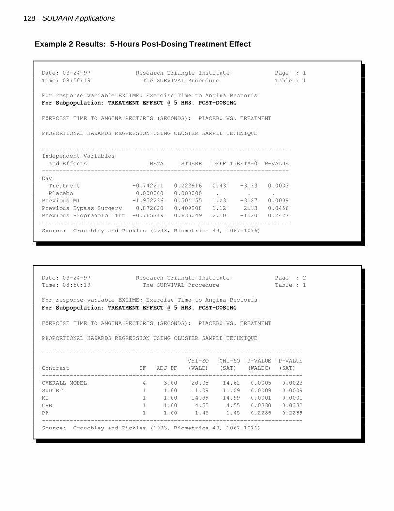
128 SUDAAN Applications
Example 2 Results: 5-Hours Post-Dosing Treatment Effect
Date: 03-24-97 Research Triangle Institute Page : 1 Time: 08:50:19 The SURVIVAL Procedure Table : 1
For response variable EXTIME: Exercise Time to Angina Pectoris For Subpopulation: TREATMENT EFFECT @ 5 HRS. POST-DOSING
EXERCISE TIME TO ANGINA PECTORIS (SECONDS): PLACEBO VS. TREATMENT PROPORTIONAL HAZARDS REGRESSION USING CLUSTER SAMPLE TECHNIQUE
----------------------------------------------------------------------- Independent Variables and Effects BETA STDERR DEFF T:BETA=0 P-VALUE ----------------------------------------------------------------------- Day Treatment -0.742211 0.222916 0.43 -3.33 0.0033 Placebo 0.000000 0.000000 . . . Previous MI -1.952236 0.504155 1.23 -3.87 0.0009 Previous Bypass Surgery 0.872620 0.409208 1.12 2.13 0.0456 Previous Propranolol Trt -0.765749 0.636049 2.10 -1.20 0.2427 ----------------------------------------------------------------------- Source: Crouchley and Pickles (1993, Biometrics 49, 1067-1076)
Date: 03-24-97 Research Triangle Institute Page : 2 Time: 08:50:19 The SURVIVAL Procedure Table : 1
For response variable EXTIME: Exercise Time to Angina Pectoris
For Subpopulation: TREATMENT EFFECT @ 5 HRS. POST-DOSING
EXERCISE TIME TO ANGINA PECTORIS (SECONDS): PLACEBO VS. TREATMENT PROPORTIONAL HAZARDS REGRESSION USING CLUSTER SAMPLE TECHNIQUE
--------------------------------------------------------------------------- CHI-SQ CHI-SQ P-VALUE P-VALUE Contrast DF ADJ DF (WALD) (SAT) (WALDC) (SAT) --------------------------------------------------------------------------- OVERALL MODEL 4 3.00 20.05 14.62 0.0005 0.0023 SUDTRT 1 1.00 11.09 11.09 0.0009 0.0009 MI 1 1.00 14.99 14.99 0.0001 0.0001 CAB 1 1.00 4.55 4.55 0.0330 0.0332 PP 1 1.00 1.45 1.45 0.2286 0.2289 --------------------------------------------------------------------------- Source: Crouchley and Pickles (1993, Biometrics 49, 1067-1076)

Example 2: Repeated Exercise Times in a Clinical Trial 129
Example 2 Results: 5-Hours Post-Dosing Treatment Effect
Date: 03-24-97 Research Triangle Institute Page : 3 Time: 08:50:19 The SURVIVAL Procedure Table : 1
For response variable EXTIME: Exercise Time to Angina Pectoris For Subpopulation: TREATMENT EFFECT @ 5 HRS. POST-DOSING
EXERCISE TIME TO ANGINA PECTORIS (SECONDS): PLACEBO VS. TREATMENT
PROPORTIONAL HAZARDS REGRESSION USING CLUSTER SAMPLE TECHNIQUE
----------------------------------------------- Independent Variables Lower Upper and Effects Hazards 95% 95% Ratio Limit Limit ----------------------------------------------- Day Treatment 0.48 0.30 0.76 Placebo 1.00 1.00 1.00 Previous MI 0.14 0.05 0.41 Previous Bypass Surgery 2.39 1.02 5.62 Previous Propranolol Trt 0.46 0.12 1.75 ----------------------------------------------- Source: Crouchley and Pickles (1993, Biometrics 49, 1067-1076)
SURVIVAL used CPU time : 2.86 seconds Elapsed time : 3 seconds Virtual memory : 1.06 MB

130 SUDAAN Applications
Example 3: Ordinal Outcomes in a Cross-Over Clinical Trial 131
Cross-Over Clinical Trial With Ordinal Outcomes:
Evaluation of a New Inhaler Device via a Cross-Over Clinical TrialQualitative responses in a cross-over clinical trial are often ordinal. Such responses might be, forexample, relief, slight relief, or no relief in studies of painkiller effectiveness. Due to the natureof cross-over studies, repeated measurements on the same subject are likely to be correlated. Theintra-subject correlation must be taken into account in order to make valid inferences about thetreatment effect.
Data for this example are from a two-treatment two-period crossover study conducted by 3MHealth Care Ltd (Ezzet and Whitehead, 1991) to compare the suitability of two inhalationdevices (A and B) in patients who are currently using a standard inhaler device deliveringsalbutamol. The first sequence of patients were randomized to Device A for one week (period 1)followed by Device B for another week (period 2). The second sequence of patients received thetreatments in the opposite order (Device B in period 1, Device A in period 2). Patients gave theirassessment on clarity of leaflet instructions accompanying the devices, recorded on an ordinalscale of: 1 = easy, 2 = clear only after re-reading, 3 = not very clear, and 4 = confusing.
Variables in the regression models included:
TREATMENT: A or B
PERIOD: 1 or 2.
The accompanying output contains results from the following SUDAAN procedures:
1) PROC RECORDS - contents of the data set
2) PROC CROSSTAB - descriptive statistics: distribution of the 4-level ordinaloutcome across treatment group
3) PROC MULTILOG - proportional odds and multinomial logit regression oftreatment and period effects on leaflet clarity

132 SUDAAN Applications
Structure of the Clarity Data
Patient Period Treatment Y = Clarity
1 1 1 = New 1 = Easy
1 2 2 = Standard 1 = Easy
2 1 1 1 = Easy
2 2 2 2 = Rereading
3 1 2 3 = Not Clear
3 2 1 2 = Rereading
4 1 2 4 = Confusing
4 2 1 1 = Easy
N = 572 records on the file
(286 clusters, 2 records per cluster)

Example 3: Ordinal Outcomes in a Cross-Over Clinical Trial 133
Example 3 Results:
File Contents
1 PROC RECORDS DATA="C:\\TERA\\GEEORD\\CROSS" FILETYPE=SAS CONTENTS COUNTREC NOPRINT;
SAS Record File C:\TERA\GEEORD\CROSS.SSD Variables Name Type Format Description ---------------------------------------------------------------------------- PERSON Numeric F15.3 PERSON TREAT Numeric F15.3 TREAT SEQUENCE Numeric F15.3 SEQUENCE PERIOD Numeric F15.3 PERIOD CLARITY Numeric F15.3 CLARITY
Codes and Labels for Variable TREAT: Code Label ------------- 1 Inhaler A 2 Inhaler B
Codes and Labels for Variable PERIOD: Code Label ------------- 1 1=AB 2 2=BA
Codes and Labels for Variable CLARITY: Code Label ------------- 1 Easy 2 Rereading 3 Not Clear 4 Confusing
Number of records on file : 572
RECORDS used CPU time : 0.55 seconds Elapsed time : 1 second Virtual memory : 0.75 MB
There are 572 records (one record for each person and treatment occasion) on the SAS data set. Theoutcome of interest is CLARITY of leaflet instructions, coded 1=easy, 2=rereading required, 3=notclear, and 4=confusing. SUDAAN picks up the labels for dependent and independent variables from theuser-defined LEVEL.DBS file.
In the proportional odds model, we will model the probability of increasing clarity across treatment groupand period (1 vs. 2). In the multinomial logit model, we will model the probability of being in each ofthe first 3 levels of CLARITY vs. the last.

134 SUDAAN Applications
CLARITY 1 EasyCLARITY 2 RereadingCLARITY 3 Not ClearCLARITY 4 ConfusingTREAT 1 Inhaler ATREAT 2 Inhaler BSEQUENCE 1 1=ABSEQUENCE 2 2=BA
The LEVEL.DBS file for Example 3:
Value labels for categorical variables:

Example 3: Ordinal Outcomes in a Cross-Over Clinical Trial 135
2 PROC CROSSTAB DATA="C:\\TERA\\NCHS\\CROSS" FILETYPE=SAS; 3 NEST _ONE_ PERSON; 4 WEIGHT _ONE_; 5 SUBGROUP TREAT CLARITY; 6 LEVELS 2 4; 7 TABLES TREAT*CLARITY; 8 SETENV DECWIDTH=0 COLWIDTH=10 LABWIDTH=15 COLSPCE=2; 9 PRINT NSUM/STYLE=NCHS; 10 TITLE " " "FREQUENCY DISTRIBUTION FOR INHALER DEVICE CROSS-OVER STUDY" " " "Ezzett and Whitehead, 1991" " ";
Number of observations read : 572 Weighted count : 572Number of observations skipped : 0(WEIGHT variable nonpositive)Denominator degrees of freedom : 285
Date: 03-18-97 Research Triangle Institute Page : 1 Time: 11:18:22 The CROSSTAB Procedure Table : 1
FREQUENCY DISTRIBUTION FOR INHALER DEVICE CROSS-OVER STUDY Ezzett and Whitehead, 1991 Sample Size --------------------------------------------------------------------------- TREAT CLARITY Total Easy Rereading Not Clear Confusing --------------------------------------------------------------------------- Total 572 358 189 17 8 Inhaler A 286 211 71 2 2 Inhaler B 286 147 118 15 6 ---------------------------------------------------------------------------
Example 3 Results :
The CROSSTAB procedure was used to obtain the frequency distribution of CLARITY acrosstreatment. It appears that the Inhaler B leaflet is less easy to read than that for Inhaler A.
136 SUDAAN Applications
MULTILOG Programming Statements and OptionsThe first set of MULTILOG programming statements fits the proportional odds model inSUDAAN PROC MULTILOG. The DATA option on the PROC statement specifies a SAS dataset as input. Since there is no DESIGN option specified, SUDAAN is using the defaultDESIGN=WR (with-replacement) option for variance estimation.
We will fit the following types of models:
1) SEMETHOD=ZEGER and R=INDEPENDENT Implements the GEE model-fitting technique under an independent “working”assumption and a robust variance estimator.
2) SEMETHOD=ZEGER and R=EXCHANGEABLE Implements the GEE model-fitting technique under exchangeable “working” correlationsand a robust variance estimator.
3) SEMETHOD=MODEL and R=EXCHANGEABLEWe compare the results using the robust variance estimator (SEMETHOD=ZEGER) tothe model-based, or naive, variance assumption (SEMETHOD=MODEL). WhenR=exchangeable is specified in conjunction with SEMETHOD=MODEL, variances arethen computed as if the exchangeable “working” correlation assumption were correct.
The NEST statement indicates that PERSON is the cluster variable. The WEIGHT statementindicates equal sampling weights of 1.0 for each person and measurement occasion.
In MULTILOG, the SUBGROUP statement contains the dependent variable and all covariatesthat are to be modelled as categorical covariates (with level values of 1,2,...,k), where themaximum number of levels (K) appears on the LEVELS statement.
The MODEL statement specifies the categorical dependent variable CLARITY on the left of the"=" sign (with levels 1, 2, 3, and 4), and regressors on the right. The CUMLOGIT (cumulativelogit) link specifies the proportional odds model (the GENLOGIT link comes later in the output). The CUMLOGIT link will model the log-odds that CLARITY � k, where k=1,...,K-1 (or thetendency for CLARITY to be less than confusing). The GENLOGIT link will model the log-odds that CLARITY=k vs. K (or the log-odds that CLARITY is easy, requires re-reading, or notclear vs. confusing). The CUMLOGIT option produces common slopes but separate interceptsfor each of the K-1 = 3 cutpoints, while the GENLOGIT option produces a separate logitequation (intercepts and slopes) for each of the 3 cutpoints.
The TEST statement specifies that we want the Wald chi-square statistic to be the default fortesting main effects, interactions, and user-defined contrasts. This statement is optional. Ifomitted, the Wald F statistic becomes the default. However, any default statistic can beoverridden on the PRINT statement.
The SETENV and PRINT statements are both optional, and control the printing of results (whichstatistics get printed, as well as their labels, formats, and layout).

Example 3: Ordinal Outcomes in a Cross-Over Clinical Trial 137
MULTILOG Programming Statements for the Proportional Odds Model: CUMLOGIT Link
GEE with Independent Working Correlations and Robust Variance Estimates
11 PROC MULTILOG DATA="C:\\TERA\\GEEORD\\CROSS" FILETYPE=SAS SEMETHOD=ZEGER R=INDEPENDENT;
12 NEST _ONE_ PERSON;
13 WEIGHT _ONE_;
14 SUBGROUP CLARITY TREAT PERIOD;
15 LEVELS 4 2 2;
16 MODEL CLARITY = TREAT PERIOD / CUMLOGIT;
17 TEST WALDCHI;
18 SETENV LABWIDTH=28 MAXIND=4 LINESIZE=78 PAGESIZE=60 COLSPCE=2;
19 PRINT BETA="BETA" SEBETA="STDERR" DEFT="DESIGN EFFECT" T_BETA="T:BETA=0" P_BETA="P-Value"/ RISK=ALL TESTS=DEFAULT BETAFMT=F7.4 SEBETAFMT=F6.4 T_BETAFMT=F8.2 P_BETAFMT=F7.4 DEFTFMT=F6.2 WALDCHIFMT=F6.2 WALDCHPFMT=F7.4 ORFMT=F5.2 LOWORFMT=F6.2 UPORFMT=F6.2 DFFMT=F7.0;
20 TITLE " " "PROPORTIONAL ODDS MODEL FOR INHALER DEVICE CROSS-OVER STUDY" " " "Ezzett and Whitehead, 1991";
Opened SAS data file C:\TERA\GEEORD\CROSS.SSD for reading.
Independence parameters have converged in 3 iterations
Number of observations read : 572 Weighted count: 572 Observations used in the analysis : 572 Weighted count: 572 Observations with missing values : 0 Weighted count: 0 Denominator degrees of freedom : 285
Maximum number of estimable parameters for the model is 5
File C:\TERA\GEEORD\CROSS.SSD contains 286 Clusters Maximum cluster size is 2 records Minimum cluster size is 2 records
Sample and Population Counts for Response Variable CLARITY Easy : Sample Count 358 Population Count 358 Rereading: Sample Count 189 Population Count 189 Not Clear: Sample Count 17 Population Count 17 Confusing: Sample Count 8 Population Count 8

138 SUDAAN Applications
CLARITY is the outcome variable in the model, while TREAT and PERIOD are covariates. There are 572 records on the file, corresponding to 286 clusters, with a minimum and maximumcluster size of 2 (since this is a 2-period crossover design). There are no missing values in thethe data set and no SUBPOPN statement to subset the analysis, so all observations on the file areused in fitting the model. SUDAAN displays the frequency distribution of the response in thedata and the number of iterations needed to estimate the regression coefficients.

log prob(Y�k)prob(Y>k)
0.11k1 � 2.77k2 � 3.95k3 � 1.01# TREAT 0.1512# P E RIO D
Example 3: Ordinal Outcomes in a Cross-Over Clinical Trial 139
Example 3 Results:
Proportional Odds Model: CUMLOGIT LinkGEE with Independent Working Correlations and Robust Variance Estimates
Date: 03-18-97 Research Triangle Institute Page : 1 Time: 11:18:22 The MULTILOG Procedure Table : 1
Variance Estimation Method: Robust (Zeger-Liang, 1986) Working Correlations: Independent Link Function: Cumulative Logit Response variable CLARITY: CLARITY
PROPORTIONAL ODDS MODEL FOR INHALER DEVICE CROSS-OVER STUDY
Ezzett and Whitehead, 1991
------------------------------------------------------------------------ Independent Variables and DESIGN Effects BETA STDERR EFFECT T:BETA=0 P-Value ------------------------------------------------------------------------ CLARITY (cum-logit) Intercept 1: Easy 0.1110 0.1383 0.88 0.80 0.4229 Intercept 2: Rereading 2.7656 0.2357 1.03 11.74 0.0000 Intercept 3: Not Clear 3.9464 0.3638 0.95 10.85 0.0000 TREAT Inhaler A 1.0137 0.1566 0.78 6.47 0.0000 Inhaler B 0.0000 0.0000 . . . PERIOD 1=AB -0.1512 0.1565 0.80 -0.97 0.3347 2=BA 0.0000 0.0000 . . . ------------------------------------------------------------------------
The estimated regression coefficients for the proportional odds model indicate that Inhaler A issignificantly clearer in its leaflet instructions than Inhaler B (p=0.0000, t-test). This is reflectedin the positive regression coefficient estimate (1.0137) and in the estimated odds ratio on the nextpage (2.76). In other words, the odds of being � any response level k are increased almost 3-foldover Inhaler B. Note the 3 intercept terms in the model are non-decreasing because they arecumulative over the categories of the response (i.e., intercept 1 = easy; 2 = easy or rereadingrequired; 3 = easy, rereading, or not clear). The fitted proportional odds model is as follows:
where TREAT and PERIOD are converted to 0-1 indicator variables because of their appearanceon the SUBGROUP statement.
Note the design effect of 0.78 for the treatment parameter. We expect design effects less than1.0 for treatment parameters nested within the cluster, as occurs in many repeated measuresdesigns. This indicates that an improvement in precision was obtained because of the cross-overdesign and that SUDAAN was able to recognize this gain.

140 SUDAAN Applications
Example 3 Results:
Proportional Odds Model: CUMLOGIT LinkGEE with Independent Working Correlations and Robust Variance Estimates
Date: 03-18-97 Research Triangle Institute Page : 2 Time: 11:18:22 The MULTILOG Procedure Table : 1
Variance Estimation Method: Robust (Zeger-Liang, 1986) Working Correlations: Independent Link Function: Cumulative Logit Response variable CLARITY: CLARITY
PROPORTIONAL ODDS MODEL FOR INHALER DEVICE CROSS-OVER STUDY
Ezzett and Whitehead, 1991
------------------------------------------------------ Contrast Degrees P-value of Wald Wald Freedom ChiSq ChiSq ------------------------------------------------------ OVERALL MODEL 5 272.62 0.0000 MODEL MINUS INTERCEPT 2 42.13 0.0000 TREAT 1 41.88 0.0000 PERIOD 1 0.93 0.3338 ------------------------------------------------------

Example 3: Ordinal Outcomes in a Cross-Over Clinical Trial 141
Example 3 Results:
Proportional Odds Model: CUMLOGIT LinkGEE with Independent Working Correlations and Robust Variance Estimates
Date: 03-18-97 Research Triangle Institute Page : 3 Time: 11:18:22 The MULTILOG Procedure Table : 1
Variance Estimation Method: Robust (Zeger-Liang, 1986) Working Correlations: Independent Link Function: Cumulative Logit Response variable CLARITY: CLARITY
PROPORTIONAL ODDS MODEL FOR INHALER DEVICE CROSS-OVER STUDY
Ezzett and Whitehead, 1991
--------------------------------------------------- Independent Variables and Lower Upper Effects Odds 95% 95% Ratio Limit Limit --------------------------------------------------- CLARITY (cum-logit) Intercept 1: Easy 1.12 0.85 1.47 Intercept 2: Rereading 15.89 9.99 25.26 Intercept 3: Not Clear 51.75 25.30 105.86 TREAT Inhaler A 2.76 2.03 3.75 Inhaler B 1.00 1.00 1.00 PERIOD 1=AB 0.86 0.63 1.17 2=BA 1.00 1.00 1.00 ---------------------------------------------------
MULTILOG used CPU time : 4.44 seconds Elapsed time : 5 seconds Virtual memory : 1.11 MB
This output contains the main effects tests for the proportional odds model, in addition to theestimated odds ratios and their 95% confidence limits.

142 SUDAAN Applications
Example 3 Results:
MULTILOG Programming Statements for the Proportional Odds Model: Exchangeable Correlations and Robust Variance Estimates
31 PROC MULTILOG DATA="C:\\TERA\\GEEORD\\CROSS" FILETYPE=SAS SEMETHOD=ZEGER R=EXCHANGE;
32 NEST _ONE_ PERSON;
33 WEIGHT _ONE_;
34 SUBGROUP CLARITY TREAT PERIOD;
35 LEVELS 4 2 2;
36 MODEL CLARITY = TREAT PERIOD / CUMLOGIT;
37 TEST WALDCHI; 38 SETENV LABWIDTH=15 LINESIZE=78 PAGESIZE=60;
39 PRINT RHO / RHOFMT=F10.4;
40 SETENV LABWIDTH=28 MAXIND=4 LINESIZE=78 PAGESIZE=60 COLSPCE=2;
41 PRINT BETA="BETA" SEBETA="STDERR" DEFT="DESIGN EFFECT" T_BETA="T:BETA=0" P_BETA="P-Value"/ RISK=ALL TESTS=DEFAULT BETAFMT=F7.4 SEBETAFMT=F6.4 T_BETAFMT=F8.2 P_BETAFMT=F7.4 DEFTFMT=F6.2 WALDCHIFMT=F6.2 WALDCHPFMT=F7.4 ORFMT=F5.2 LOWORFMT=F6.2 UPORFMT=F6.2 DFFMT=F7.0;
42 TITLE " " "PROPORTIONAL ODDS MODEL FOR INHALER DEVICE CROSS-OVER STUDY" " " "Ezzett and Whitehead, 1991";
Continued on next page...
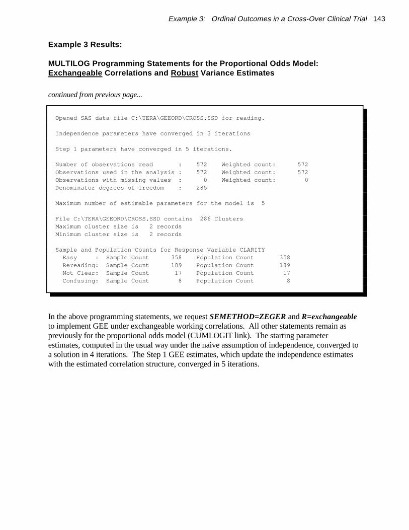
Example 3: Ordinal Outcomes in a Cross-Over Clinical Trial 143
Example 3 Results:
MULTILOG Programming Statements for the Proportional Odds Model: Exchangeable Correlations and Robust Variance Estimates
continued from previous page...
Opened SAS data file C:\TERA\GEEORD\CROSS.SSD for reading.
Independence parameters have converged in 3 iterations
Step 1 parameters have converged in 5 iterations.
Number of observations read : 572 Weighted count: 572 Observations used in the analysis : 572 Weighted count: 572 Observations with missing values : 0 Weighted count: 0 Denominator degrees of freedom : 285
Maximum number of estimable parameters for the model is 5
File C:\TERA\GEEORD\CROSS.SSD contains 286 Clusters Maximum cluster size is 2 records Minimum cluster size is 2 records
Sample and Population Counts for Response Variable CLARITY Easy : Sample Count 358 Population Count 358 Rereading: Sample Count 189 Population Count 189 Not Clear: Sample Count 17 Population Count 17 Confusing: Sample Count 8 Population Count 8
In the above programming statements, we request SEMETHOD=ZEGER and R=exchangeableto implement GEE under exchangeable working correlations. All other statements remain aspreviously for the proportional odds model (CUMLOGIT link). The starting parameterestimates, computed in the usual way under the naive assumption of independence, converged toa solution in 4 iterations. The Step 1 GEE estimates, which update the independence estimateswith the estimated correlation structure, converged in 5 iterations.

( Yi1 s , Yi1 t )( Yi2 s , Yi2 t )
144 SUDAAN Applications
Example 3 Results:
Proportional Odds Model: CUMLOGIT LinkGEE with Exchangeable Working Correlations and Robust Variance Estimates
Date: 03-18-97 Research Triangle Institute Page : 1 Time: 11:18:22 The MULTILOG Procedure Table : 1
Variance Estimation Method: Robust (Zeger-Liang, 1986) Working Correlations: Exchangeable Link Function: Cumulative Logit Response variable CLARITY: CLARITY
PROPORTIONAL ODDS MODEL FOR INHALER DEVICE CROSS-OVER STUDY
Ezzett and Whitehead, 1991 Correlation Matrix ------------------------------------------------------ CLARITY CLARITY Easy Rereading Not Clear ------------------------------------------------------ Easy 0.2156 Rereading -0.1975 0.2069 Not Clear -0.0564 -0.0168 0.1427 ------------------------------------------------------
The estimated correlation structure is contained in the above table. Note that for a 4-levelresponse variable, a cluster size of 2, and an exchangeable correlation model, there are exactly 6unique correlation estimates. SUDAAN prints the lower portion of the symmetric 3-by-3 matrix. These estimates indicate that the correlation between the “Easy to Read” categories on bothtreatments was 0.2156, and the correlation between the “Rereading Required”categories on both treatments was 0.2069. Therefore, the most frequently occuringpairs are identical outcomes. The smaller negative correlations indicate that crossing responsecategories from Inhaler A to B is not as likely as remaining in the same response category oneach treatment.

Example 3: Ordinal Outcomes in a Cross-Over Clinical Trial 145
Example 3 Results:
Proportional Odds Model: CUMLOGIT LinkGEE with Exchangeable Working Correlations and Robust Variance Estimates
Date: 03-18-97 Research Triangle Institute Page : 2 Time: 11:18:22 The MULTILOG Procedure Table : 1
Variance Estimation Method: Robust (Zeger-Liang, 1986) Working Correlations: Exchangeable Link Function: Cumulative Logit Response variable CLARITY: CLARITY
PROPORTIONAL ODDS MODEL FOR INHALER DEVICE CROSS-OVER STUDY
Ezzett and Whitehead, 1991
--------------------------------------------------------------- Independent Variables and Effects BETA STDERR T:BETA=0 P-Value --------------------------------------------------------------- CLARITY (cum-logit) Intercept 1: Easy 0.1085 0.1379 0.79 0.4320 Intercept 2: Rereading 2.7424 0.2344 11.70 0.0000 Intercept 3: Not Clear 3.9568 0.3639 10.87 0.0000 TREAT Inhaler A 1.0140 0.1562 6.49 0.0000 Inhaler B 0.0000 0.0000 . . PERIOD 1=AB -0.1531 0.1556 -0.98 0.3258 2=BA 0.0000 0.0000 . . ---------------------------------------------------------------
This table contains the regression coefficient estimates under the exchangeable correlationstructure. We see that the regression estimates are slightly larger and the variance estimates areslightly smaller compared to the independence working assumption shown previously. However,the results are qualitatively the same. Inhaler A is significantly clearer in its leaflet instructionsthan Inhaler B. Both working assumptions are valid no matter what the true correlation structuresince SUDAAN is using the robust variance estimates (SEMETHOD=ZEGER) for computingvariance and testing hypotheses.

146 SUDAAN Applications
Example 3 Results:
Proportional Odds Model: CUMLOGIT LinkGEE with Exchangeable Working Correlations and Robust Variance Estimates
Date: 03-18-97 Research Triangle Institute Page : 3 Time: 11:18:22 The MULTILOG Procedure Table : 1
Variance Estimation Method: Robust (Zeger-Liang, 1986) Working Correlations: Exchangeable Link Function: Cumulative Logit Response variable CLARITY: CLARITY
PROPORTIONAL ODDS MODEL FOR INHALER DEVICE CROSS-OVER STUDY
Ezzett and Whitehead, 1991 ------------------------------------------------------ Contrast Degrees P-value of Wald Wald Freedom ChiSq ChiSq ------------------------------------------------------ OVERALL MODEL 5 272.33 0.0000 MODEL MINUS INTERCEPT 2 42.39 0.0000 TREAT 1 42.16 0.0000 PERIOD 1 0.97 0.3250 ------------------------------------------------------
This table summarizes the main effects tests under the exchangeable correlation “working”assumption. Again, these results are qualitatively similar to the “working” independence modelwith robust variance estimates.

Example 3: Ordinal Outcomes in a Cross-Over Clinical Trial 147
Example 3 Results:
Proportional Odds Model: CUMLOGIT LinkGEE with Exchangeable Working Correlations and Robust Variance Estimates
Date: 03-18-97 Research Triangle Institute Page : 4 Time: 11:18:22 The MULTILOG Procedure Table : 1
Variance Estimation Method: Robust (Zeger-Liang, 1986) Working Correlations: Exchangeable Link Function: Cumulative Logit Response variable CLARITY: CLARITY
PROPORTIONAL ODDS MODEL FOR INHALER DEVICE CROSS-OVER STUDY
Ezzett and Whitehead, 1991
--------------------------------------------------- CLARITY (cum-logit), Independent Variables and Lower Upper Effects Odds 95% 95% Ratio Limit Limit --------------------------------------------------- CLARITY (cum-logit) Intercept 1: Easy 1.11 0.85 1.46 Intercept 2: Rereading 15.52 9.79 24.62 Intercept 3: Not Clear 52.29 25.56 106.99 TREAT Inhaler A 2.76 2.03 3.75 Inhaler B 1.00 1.00 1.00 PERIOD 1=AB 0.86 0.63 1.17 2=BA 1.00 1.00 1.00 ---------------------------------------------------
MULTILOG used CPU time : 11.91 seconds Elapsed time : 12 seconds Virtual memory : 1.14 MB
These odds ratios and 95% confidence limits for the exchangeable “working” assumption areidentical to the independence “working” model. Modelling the correlations underexchangeability did not significantly improve the efficiency of the parameter estimates in thisexample.

M 10 M 1
0 [D ��V 1D ]1
D 0%i / 0� %i
148 SUDAAN Applications
Example 3 Results:
GEE Under Exchangeable Working CorrelationsModel-Based (Naive) Variance Estimation
Below are results from the exchangeable correlation model using the model-based or naivevariance-covariance matrix of the estimated regression coefficients. The model-based varianceis the matrix, or the outside portion of the robust variance estimate: = ,where is the vector of first partial derivatives of the response probabilities withrespect to the regression coefficients ��. In this case, the naive variance estimate is computed as ifthe exchangeable “working” correlation assumption were correct. Since this is close to truthfor litter data, we will see that results are essentially the same as with the robust varianceestimator. To obtain the model-based results, we specify SEMETHOD=MODEL on the PROCstatement.
43 PROC MULTILOG DATA="C:\\TERA\\GEEORD\\CROSS" FILETYPE=SAS SEMETHOD=MODEL R=EXCHANGE;
44 NEST _ONE_ PERSON;
45 WEIGHT _ONE_;
46 SUBGROUP CLARITY TREAT PERIOD;
47 LEVELS 4 2 2;
48 MODEL CLARITY = TREAT PERIOD / CUMLOGIT;
49 TEST WALDCHI;
50 SETENV LABWIDTH=15 LINESIZE=78 PAGESIZE=60;
51 PRINT RHO / RHOFMT=F10.4;
52 SETENV LABWIDTH=28 MAXIND=4 LINESIZE=78 PAGESIZE=60 COLSPCE=2;
53 PRINT BETA="BETA" SEBETA="STDERR" DEFT="DESIGN EFFECT" T_BETA="T:BETA=0" P_BETA="P-Value"/ RISK=ALL TESTS=DEFAULT BETAFMT=F7.4 SEBETAFMT=F6.4 T_BETAFMT=F8.2 P_BETAFMT=F7.4 DEFTFMT=F6.2 WALDCHIFMT=F6.2 WALDCHPFMT=F7.4 ORFMT=F5.2 LOWORFMT=F6.2 UPORFMT=F6.2 DFFMT=F7.0;
54 TITLE " " "PROPORTIONAL ODDS MODEL FOR INHALER DEVICE CROSS-OVER STUDY" " " "Ezzett and Whitehead, 1991" "Model-Based Variance Estimation";
...continued next page

Example 3: Ordinal Outcomes in a Cross-Over Clinical Trial 149
Example 3 Results:
GEE Under Exchangeable Working CorrelationsModel-Based (Naive) Variance Estimation
...continued from previous page
Opened SAS data file C:\TERA\GEEORD\CROSS.SSD for reading.
Number of observations read : 572 Weighted count: 572 Observations used in the analysis : 572 Weighted count: 572 Observations with missing values : 0 Weighted count: 0 Denominator degrees of freedom : 285
Maximum number of estimable parameters for the model is 5
File C:\TERA\GEEORD\CROSS.SSD contains 286 Clusters
Maximum cluster size is 2 records Minimum cluster size is 2 records
Independence parameters have converged in 3 iterations
Step 1 parameters have converged in 5 iterations.
Sample and Population Counts for Response Variable CLARITY Easy : Sample Count 358 Population Count 358 Rereading: Sample Count 189 Population Count 189 Not Clear: Sample Count 17 Population Count 17 Confusing: Sample Count 8 Population Count 8
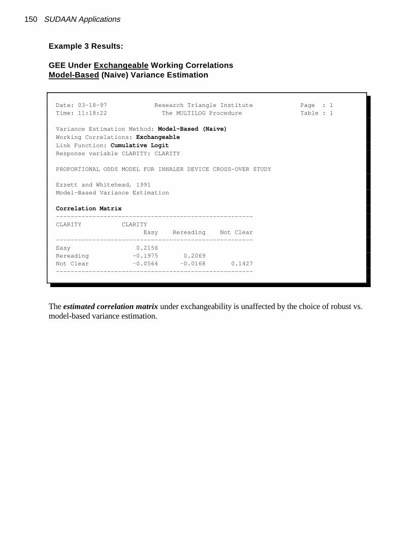
150 SUDAAN Applications
Example 3 Results:
GEE Under Exchangeable Working CorrelationsModel-Based (Naive) Variance Estimation
Date: 03-18-97 Research Triangle Institute Page : 1 Time: 11:18:22 The MULTILOG Procedure Table : 1
Variance Estimation Method: Model-Based (Naive) Working Correlations: Exchangeable Link Function: Cumulative Logit Response variable CLARITY: CLARITY
PROPORTIONAL ODDS MODEL FOR INHALER DEVICE CROSS-OVER STUDY
Ezzett and Whitehead, 1991 Model-Based Variance Estimation Correlation Matrix ------------------------------------------------------ CLARITY CLARITY Easy Rereading Not Clear ------------------------------------------------------ Easy 0.2156 Rereading -0.1975 0.2069 Not Clear -0.0564 -0.0168 0.1427 ------------------------------------------------------
The estimated correlation matrix under exchangeability is unaffected by the choice of robust vs.model-based variance estimation.

Example 3: Ordinal Outcomes in a Cross-Over Clinical Trial 151
Example 3 Results:
GEE Under Exchangeable Working CorrelationsModel-Based (Naive) Variance Estimation
Date: 03-18-97 Research Triangle Institute Page : 2 Time: 11:18:22 The MULTILOG Procedure Table : 1
Variance Estimation Method: Model-Based (Naive) Working Correlations: Exchangeable Link Function: Cumulative Logit Response variable CLARITY: CLARITY
PROPORTIONAL ODDS MODEL FOR INHALER DEVICE CROSS-OVER STUDY
Ezzett and Whitehead, 1991 Model-Based Variance Estimation
---------------------------------------------------------------- Independent Variables and Effects BETA STDERR T:BETA=0 P-Value ---------------------------------------------------------------- CLARITY (cum-logit) Intercept 1: Easy 0.1085 0.1415 0.77 0.4437 Intercept 2: Rereading 2.7424 0.2363 11.61 0.0000 Intercept 3: Not Clear 3.9568 0.3510 11.27 0.0000 TREAT Inhaler A 1.0140 0.1577 6.43 0.0000 Inhaler B 0.0000 0.0000 . . PERIOD 1=AB -0.1531 0.1555 -0.98 0.3256 2=BA 0.0000 0.0000 . . ----------------------------------------------------------------
Here we have the estimated regression coefficients computed under exchangeability and theestiamted standard errors as if the exchangeable working asssumption were correct. The standarderrors are roughly the same as with the robust variance estimator for these data, indicating thatthe exchangeable correlation assumption is close to truth.

152 SUDAAN Applications
Example 3 Results:
GEE Under Exchangeable Working CorrelationsModel-Based (Naive) Variance Estimation
Date: 03-18-97 Research Triangle Institute Page : 3 Time: 11:18:22 The MULTILOG Procedure Table : 1
Variance Estimation Method: Model-Based (Naive) Working Correlations: Exchangeable Link Function: Cumulative Logit Response variable CLARITY: CLARITY
PROPORTIONAL ODDS MODEL FOR INHALER DEVICE CROSS-OVER STUDY
Ezzett and Whitehead, 1991 Model-Based Variance Estimation
------------------------------------------------------ Contrast Degrees P-value of Wald Wald Freedom ChiSq ChiSq ------------------------------------------------------ OVERALL MODEL 5 271.76 0.0000 MODEL MINUS INTERCEPT 2 42.17 0.0000 TREAT 1 41.33 0.0000 PERIOD 1 0.97 0.3248 ------------------------------------------------------
Here we have the main effects tests computed under exchangeability, using the model-basedvariance approach. Results are essentially the same as with the robust variance estimator.

Example 3: Ordinal Outcomes in a Cross-Over Clinical Trial 153
Example 3 Results:
GEE Under Exchangeable Working CorrelationsModel-Based (Naive) Variance Estimation
Date: 03-18-97 Research Triangle Institute Page : 4 Time: 11:18:22 The MULTILOG Procedure Table : 1
Variance Estimation Method: Model-Based (Naive) Working Correlations: Exchangeable Link Function: Cumulative Logit Response variable CLARITY: CLARITY
PROPORTIONAL ODDS MODEL FOR INHALER DEVICE CROSS-OVER STUDY
Ezzett and Whitehead, 1991 Model-Based Variance Estimation
--------------------------------------------------- CLARITY (cum-logit), Independent Variables and Lower Upper Effects Odds 95% 95% Ratio Limit Limit --------------------------------------------------- CLARITY (cum-logit) Intercept 1: Easy 1.11 0.84 1.47 Intercept 2: Rereading 15.52 9.75 24.71 Intercept 3: Not Clear 52.29 26.21 104.31 TREAT Inhaler A 2.76 2.02 3.76 Inhaler B 1.00 1.00 1.00 PERIOD 1=AB 0.86 0.63 1.17 2=BA 1.00 1.00 1.00 ---------------------------------------------------
MULTILOG used CPU time : 10.60 seconds Elapsed time : 11 seconds Virtual memory : 1.14 MB
Here we have the estimated odds ratios and their 95% confidence limits computed underexchangeability, using the model-based variance approach. Odds ratios are unaffected by thechoice of robust vs. model-based variance estimates, and estimated confidence limits areessentially the same as with the robust variance estimator.
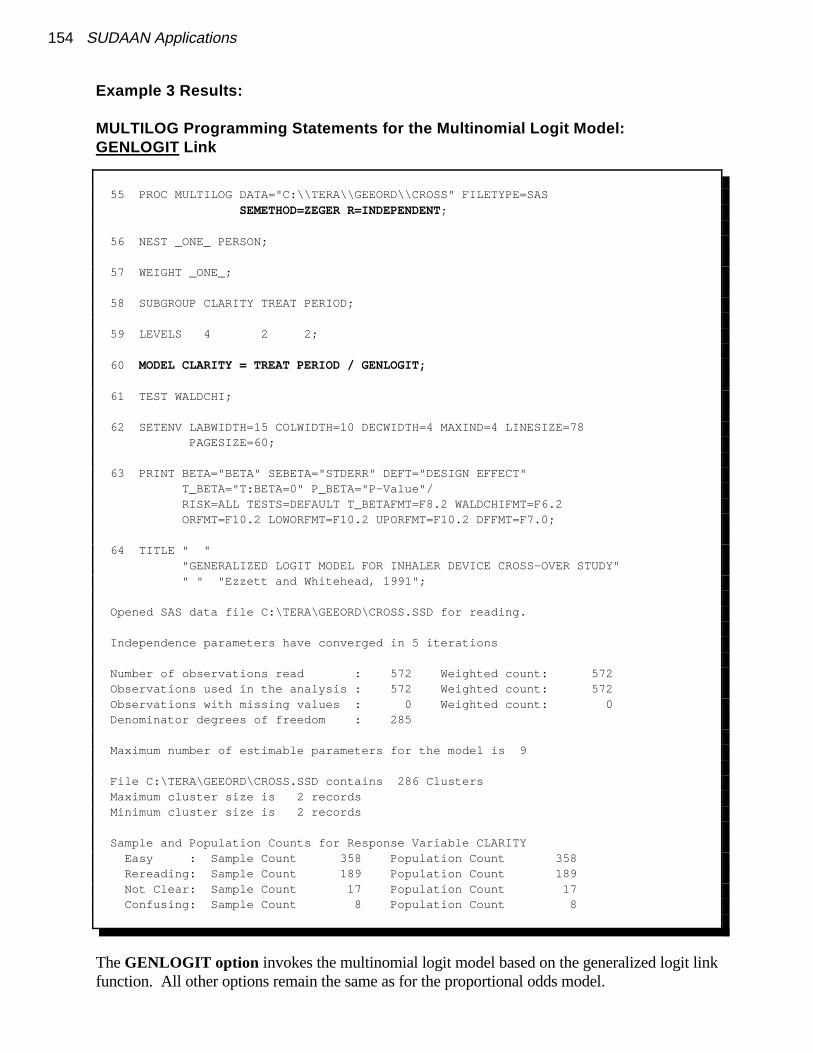
154 SUDAAN Applications
Example 3 Results:
MULTILOG Programming Statements for the Multinomial Logit Model: GENLOGIT Link
55 PROC MULTILOG DATA="C:\\TERA\\GEEORD\\CROSS" FILETYPE=SAS SEMETHOD=ZEGER R=INDEPENDENT;
56 NEST _ONE_ PERSON;
57 WEIGHT _ONE_;
58 SUBGROUP CLARITY TREAT PERIOD;
59 LEVELS 4 2 2;
60 MODEL CLARITY = TREAT PERIOD / GENLOGIT;
61 TEST WALDCHI;
62 SETENV LABWIDTH=15 COLWIDTH=10 DECWIDTH=4 MAXIND=4 LINESIZE=78 PAGESIZE=60;
63 PRINT BETA="BETA" SEBETA="STDERR" DEFT="DESIGN EFFECT" T_BETA="T:BETA=0" P_BETA="P-Value"/ RISK=ALL TESTS=DEFAULT T_BETAFMT=F8.2 WALDCHIFMT=F6.2 ORFMT=F10.2 LOWORFMT=F10.2 UPORFMT=F10.2 DFFMT=F7.0;
64 TITLE " " "GENERALIZED LOGIT MODEL FOR INHALER DEVICE CROSS-OVER STUDY" " " "Ezzett and Whitehead, 1991";
Opened SAS data file C:\TERA\GEEORD\CROSS.SSD for reading.
Independence parameters have converged in 5 iterations
Number of observations read : 572 Weighted count: 572 Observations used in the analysis : 572 Weighted count: 572 Observations with missing values : 0 Weighted count: 0 Denominator degrees of freedom : 285
Maximum number of estimable parameters for the model is 9
File C:\TERA\GEEORD\CROSS.SSD contains 286 Clusters Maximum cluster size is 2 records Minimum cluster size is 2 records
Sample and Population Counts for Response Variable CLARITY Easy : Sample Count 358 Population Count 358 Rereading: Sample Count 189 Population Count 189 Not Clear: Sample Count 17 Population Count 17 Confusing: Sample Count 8 Population Count 8
The GENLOGIT option invokes the multinomial logit model based on the generalized logit linkfunction. All other options remain the same as for the proportional odds model.

Example 3: Ordinal Outcomes in a Cross-Over Clinical Trial 155
Example 3 Results:
Multinomial Logit Model: GENLOGIT Link
GEE with Independent Working Correlations and Robust Variance Estimates
Date: 03-18-97 Research Triangle Institute Page : 1 Time: 11:18:22 The MULTILOG Procedure Table : 1
Variance Estimation Method: Robust (Zeger-Liang, 1986) Working Correlations: Independent Link Function: Generalized Logit Response variable CLARITY: CLARITY
GENERALIZED LOGIT MODEL FOR INHALER DEVICE CROSS-OVER STUDY
Ezzett and Whitehead, 1991 ----------------------------------------------------------------------------- | CLARITY (log- | | Independent Variables and Effects | odds) | | Intercept | TREAT = | TREAT = | | | | | Inhaler A | Inhaler B | ----------------------------------------------------------------------------- | | | | | | | Easy vs | BETA | 3.5099 | 1.4615 | 0.0000 | | Confusing | STDERR | 0.6858 | 0.8254 | 0.0000 | | | DESIGN EFFECT | 1.2232 | 1.0037 | . | | | T:BETA=0 | 5.12 | 1.77 | . | | | P-Value | 0.0000 | 0.0777 | . | ----------------------------------------------------------------------------- | | | | | | | Rereading vs | BETA | 3.2510 | 0.5919 | 0.0000 | | Confusing | STDERR | 0.6908 | 0.8311 | 0.0000 | | | DESIGN EFFECT | 1.2281 | 1.0015 | . | | | T:BETA=0 | 4.71 | 0.71 | . | | | P-Value | 0.0000 | 0.4769 | . | ----------------------------------------------------------------------------- | | | | | | | Not Clear vs | BETA | 1.0089 | -0.9159 | 0.0000 | | Confusing | STDERR | 0.7634 | 1.1557 | 0.0000 | | | DESIGN EFFECT | 1.1092 | 1.0830 | . | | | T:BETA=0 | 1.32 | -0.79 | . | | | P-Value | 0.1874 | 0.4287 | . | -----------------------------------------------------------------------------
-continued-

log%EASY
%C ON FUSI NG
3.51 � 1.46# TREAT 0.5593# PERIOD
156 SUDAAN Applications
Example 3 Results:
Multinomial Logit Model: GENLOGIT Link
GEE with Independent Working Correlations and Robust Variance Estimates
Date: 03-18-97 Research Triangle Institute Page : 2 Time: 11:18:22 The MULTILOG Procedure Table : 1
Variance Estimation Method: Robust (Zeger-Liang, 1986) Working Correlations: Independent Link Function: Generalized Logit Response variable CLARITY: CLARITY
GENERALIZED LOGIT MODEL FOR INHALER DEVICE CROSS-OVER STUDY
Ezzett and Whitehead, 1991 ---------------------------------------------------------------- | CLARITY (log- | | Independent Variables and Effects | odds) | | PERIOD = | PERIOD = | | | | 1=AB | 2=BA | ---------------------------------------------------------------- | | | | | | Easy vs | BETA | -0.5593 | 0.0000 | | Confusing | STDERR | 0.7401 | 0.0000 | | | DESIGN EFFECT | 0.9995 | . | | | T:BETA=0 | -0.76 | . | | | P-Value | 0.4505 | . | ---------------------------------------------------------------- | | | | | | Rereading vs | BETA | -0.4805 | 0.0000 | | Confusing | STDERR | 0.7456 | 0.0000 | | | DESIGN EFFECT | 1.0016 | . | | | T:BETA=0 | -0.64 | . | | | P-Value | 0.5198 | . | ---------------------------------------------------------------- | | | | | | Not Clear vs | BETA | -0.1527 | 0.0000 | | Confusing | STDERR | 0.8992 | 0.0000 | | | DESIGN EFFECT | 1.0411 | . | | | T:BETA=0 | -0.17 | . | | | P-Value | 0.8653 | . | ----------------------------------------------------------------
In this and the previous box we have the estimated regression coefficient vector and relatedstatistics. Note that we now have 3 separate logit equations. So, for example, the logit equationfor CLARITY = Easy vs. CLARITY = Confusing is as follows:
where TREAT and PERIOD are converted to 0-1 indicator variables because of their appearanceon the SUBGROUP statement. The treatment effect appears to be largest when comparing theEasy vs. Confusing categories.

Example 3: Ordinal Outcomes in a Cross-Over Clinical Trial 157
Example 3 Results:
Multinomial Logit Model: GENLOGIT Link
GEE with Independent Working Correlations and Robust Variance Estimates
Date: 03-18-97 Research Triangle Institute Page : 3 Time: 11:18:22 The MULTILOG Procedure Table : 1
Variance Estimation Method: Robust (Zeger-Liang, 1986) Working Correlations: Independent Link Function: Generalized Logit Response variable CLARITY: CLARITY
GENERALIZED LOGIT MODEL FOR INHALER DEVICE CROSS-OVER STUDY
Ezzett and Whitehead, 1991
----------------------------------------------- Contrast Degrees of Wald P-value Freedom ChiSq Wald ChiSq ----------------------------------------------- OVERALL MODEL 9 233.14 0.0000 MODEL MINUS INTERCEPT 6 45.27 0.0000 INTERCEPT . . . TREAT 3 39.88 0.0000 PERIOD 3 1.44 0.6962 -----------------------------------------------
The treatment effect (now with 3 degress of freedom in the multinomial logit model) isstatistically significant, as in the proportional odds model.

158 SUDAAN Applications
Example 3 Results:
Multinomial Logit Model: GENLOGIT Link
GEE with Independent Working Correlations and Robust Variance Estimates
Date: 03-18-97 Research Triangle Institute Page : 4 Time: 11:18:22 The MULTILOG Procedure Table : 1
Variance Estimation Method: Robust (Zeger-Liang, 1986) Working Correlations: Independent Link Function: Generalized Logit Response variable CLARITY: CLARITY
GENERALIZED LOGIT MODEL FOR INHALER DEVICE CROSS-OVER STUDY
Ezzett and Whitehead, 1991 ----------------------------------------------------------------------------- | CLARITY (log- | | Independent Variables and Effects | odds) | | Intercept | TREAT = | TREAT = | | | | | Inhaler A | Inhaler B | ----------------------------------------------------------------------------- | | | | | | | Easy vs | Odds Ratio | 33.44 | 4.31 | 1.00 | | Confusing | Lower 95% Limit | 8.68 | 0.85 | 1.00 | | | Upper 95% Limit | 128.91 | 21.87 | 1.00 | ----------------------------------------------------------------------------- | | | | | | | Rereading vs | Odds Ratio | 25.82 | 1.81 | 1.00 | | Confusing | Lower 95% Limit | 6.63 | 0.35 | 1.00 | | | Upper 95% Limit | 100.47 | 9.27 | 1.00 | ----------------------------------------------------------------------------- | | | | | | | Not Clear vs | Odds Ratio | 2.74 | 0.40 | 1.00 | | Confusing | Lower 95% Limit | 0.61 | 0.04 | 1.00 | | | Upper 95% Limit | 12.31 | 3.89 | 1.00 | -----------------------------------------------------------------------------
- continued -
The estimated odds of being in the EASY vs. CONFUSING categories is increased over 4-fold forInhaler A vs. B.

Example 3: Ordinal Outcomes in a Cross-Over Clinical Trial 159
Example 3 Results:
Multinomial Logit Model: GENLOGIT Link
GEE with Independent Working Correlations and Robust Variance Estimates
Date: 03-18-97 Research Triangle Institute Page : 5 Time: 11:18:22 The MULTILOG Procedure Table : 1
Variance Estimation Method: Robust (Zeger-Liang, 1986) Working Correlations: Independent Link Function: Generalized Logit Response variable CLARITY: CLARITY
GENERALIZED LOGIT MODEL FOR INHALER DEVICE CROSS-OVER STUDY
Ezzett and Whitehead, 1991 ---------------------------------------------------------------- | CLARITY (log- | | Independent Variables and Effects | odds) | | PERIOD = | PERIOD = | | | | 1=AB | 2=BA | ---------------------------------------------------------------- | | | | | | Easy vs | Odds Ratio | 0.57 | 1.00 | | Confusing | Lower 95% Limit | 0.13 | 1.00 | | | Upper 95% Limit | 2.45 | 1.00 | ---------------------------------------------------------------- | | | | | | Rereading vs | Odds Ratio | 0.62 | 1.00 | | Confusing | Lower 95% Limit | 0.14 | 1.00 | | | Upper 95% Limit | 2.68 | 1.00 | ---------------------------------------------------------------- | | | | | | Not Clear vs | Odds Ratio | 0.86 | 1.00 | | Confusing | Lower 95% Limit | 0.15 | 1.00 | | | Upper 95% Limit | 5.03 | 1.00 | ---------------------------------------------------------------- MULTILOG used CPU time : 5.50 seconds Elapsed time : 6 seconds Virtual memory : 1.18 MB

160 SUDAAN Applications

Example 4. Continuous Outcomes in a Teratology Experiment 161
Example 4.
Teratology Experiment: Clustered Continuous DataThis example demonstrates the GEE (Zeger and Liang, 1986; Liang and Zeger, 1986) andJackknife model-fitting techniques in the context of a pre-clinical teratology experiment.
The typical teratology screening experiment involves administration of a compound to pregnantdams of a given animal species, followed by evaluation of the fetuses just prior to the end ofgestation for fetal body weight, fetal death, and various types of fetal malformations. Theexperimental groups consist of a control group and anywhere from 2 to 5 exposed groups,representing increasing dosages of the compound under test. The data for this example representfetal body weight in rats after administration of boric acid (0, 0.025, 0.05, 0.075, 0.1, or 0.2% infeed) to the dam daily during gestation. There were a total of 164 litters in the experiment(average of 27 litters per group) and anywhere from 2-14 fetuses per litter (1,302 fetuses total).
In this example, the observations on fetuses are clustered within litters. The design effectmeasures the inflation (or deflation) in variance of a sample statistic due to intraclustercorrelation beyond that expected if the data were independent. It is estimated as the ratio of thecluster sample variance obtained through GEE or Jackknife vs. independence. Design effects inthis study ranged from 3 to 6, reflecting high intralitter correlations.
To implement the GEE methods in SUDAAN, we first estimated the model parameters viaordinary least squares (OLS) with a robust variance estimate. This is the GEE linear modelwith independent “working” correlations (which we refer to as GEE-independent). The Waldchi-square test was used to evaluate the null hypothesis of no dose-related effect.
For comparison, the same linear model was also fit using:
1) GEE linear regression under exchangeable intralitter correlations, 2) linear regression with Jackknife variance estimation, and 3) ordinary least squares with no variance correction
Results for GEE-exchangeable, GEE-independent, and the Jackknife approach were essentiallythe same. For comparing the high dose to control in the linear model, the GEE-exchangeableapproach yielded a Z-statistic of -7.40, compared to a GEE-independent Z-statistic of -8.11 and aJackknife Z-statistic of -7.83. The Z-statistic which ignores clustering altogether wasmisleadingly high, -14.54. The observed design effect for the high dose vs. control regressionparameter was over 3.0 for these data, reflecting substantial intralitter correlations (estimated tobe 0.5056).
Naively ignoring the clustering of the design in both parameter and variance estimation yieldssignificant reductions (p<0.05) in body weights in dose groups as low as .05% (2nd lowest dosegroup) and marginally significant reductions (p=0.06) in the lowest dose group, while all threealternative approaches (GEE-independent, GEE-exchangeable, and Jackknife) only detectsignificant reductions in the two highest dose groups. Therefore, if we ignore intraclustercorrelations for cluster-level covariates (dose group in this study), we run the risk of detectingfalse-positive results.

162 SUDAAN Applications
Structure of the Fetal Body Weight Data
Dose Group1 = Control6 = High Dose
Litter ID Fetus ID Y = fetal bodyweight (gms)
1 1 1 3.56
1 1 2 3.20
1 1 3 4.14
1 2 1 2.99
1 2 2 3.21
6 10 1 2.11
6 10 2 3.43
6 20 1 4.88
6 20 2 3.10
6 30 1 2.67
N = 1,302 records on the file (1,302 fetuses clustered within 164 litters)

Example 4. Continuous Outcomes in a Teratology Experiment 163
Figure 1
Linear Regression for the Boric Acid Data
Exposed vs. Control Group Contrasts
ContrastModel-FittingMethod � S.E. Z P-Value
0.025% Vs. Control GEE (indep) -0.0611 0.0596 -1.03 0.3067GEE (exch corr) -0.0509 0.0622 -0.82 0.4148Jackknife -0.0611 0.0616 -0.99 0.3227Independence -0.0611 0.0332 -1.84 0.0676
0.050% Vs. Control GEE (indep) -0.0789 0.0724 -1.09 0.2777GEE (exch corr) -0.0656 0.0738 -0.89 0.3753Jackknife -0.0789 0.0752 -1.05 0.2955Independence -0.0789 0.0330 -2.39 0.0180
0.075% Vs. Control GEE (indep) -0.1219 0.0740 -1.65 0.1016GEE (exch corr) -0.1363 0.0790 -1.73 0.0864Jackknife -0.1219 0.0765 -1.59 0.1128Independence -0.1219 0.0327 -3.73 0.0003
0.10% Vs. Control GEE (indep) -0.2062 0.0627 -3.29 0.0012GEE (exch corr) -0.2409 0.0680 -3.54 0.0005Jackknife -0.2062 0.0648 -3.18 0.0018Independence -0.2062 0.0323 -6.39 0.0000
0.20% Vs. Control GEE (indep) -0.4883 0.0602 -8.11 0.0000GEE (exch corr) -0.4822 0.0651 -7.40 0.0000Jackknife -0.4883 0.0624 -7.83 0.0000Independence -0.4883 0.0336 -14.54 0.0000
GEE (independent): SUDAAN REGRESS ProcedureGEE (exchangeable): SUDAAN REGRESS ProcedureJackknife: SUDAAN REGRESS ProcedureIndependence: Standard Packages (e.g., SAS GLM)
All procedures in this table (except Independence) use a robust variance estimator.

164 SUDAAN Applications
Example 4 Results:
Descriptive StatisticsHere we present the average fetal body weight in each dose group, along with their estimatedstandard errors (using a robust variance estimate to adjust for clustering) and design effects. These design effects were in the range of 3-6, reflecting more than a tripling in the variance ofthe estimated means under the clustered design. In the program code, the DAMID variablerepresents the cluster on the NEST statement. Results show that fetal body weight is reduced inthe two highest dose groups compared to control.
1 PROC DESCRIPT DATA="c:\\tera\\examples\\boric" FILETYPE=SAS NOMARG DESIGN=WR;
2 NEST _ONE_ DAMID;
3 WEIGHT _ONE_;
4 VAR BW;
5 SUBGROUP DOSEGRP;
6 LEVELS 6;
7 SETENV LABWIDTH=30 COLWIDTH=8 LINESIZE=78 DECWIDTH=4 PAGESIZE=60;
8 PRINT NSUM="SAMPLE SIZE" MEAN="MEAN" SEMEAN="SE" DEFFMEAN="DESIGN EFFECT" / STYLE=NCHS NSUMFMT=F6.0;
9 TITLE "Fetal Body Weight in a Teratology Study";
Opened SAS data file c:\tera\examples\boric.SSD for reading.
Number of observations read : 1302 Weighted count : 1302 Denominator degrees of freedom : 163
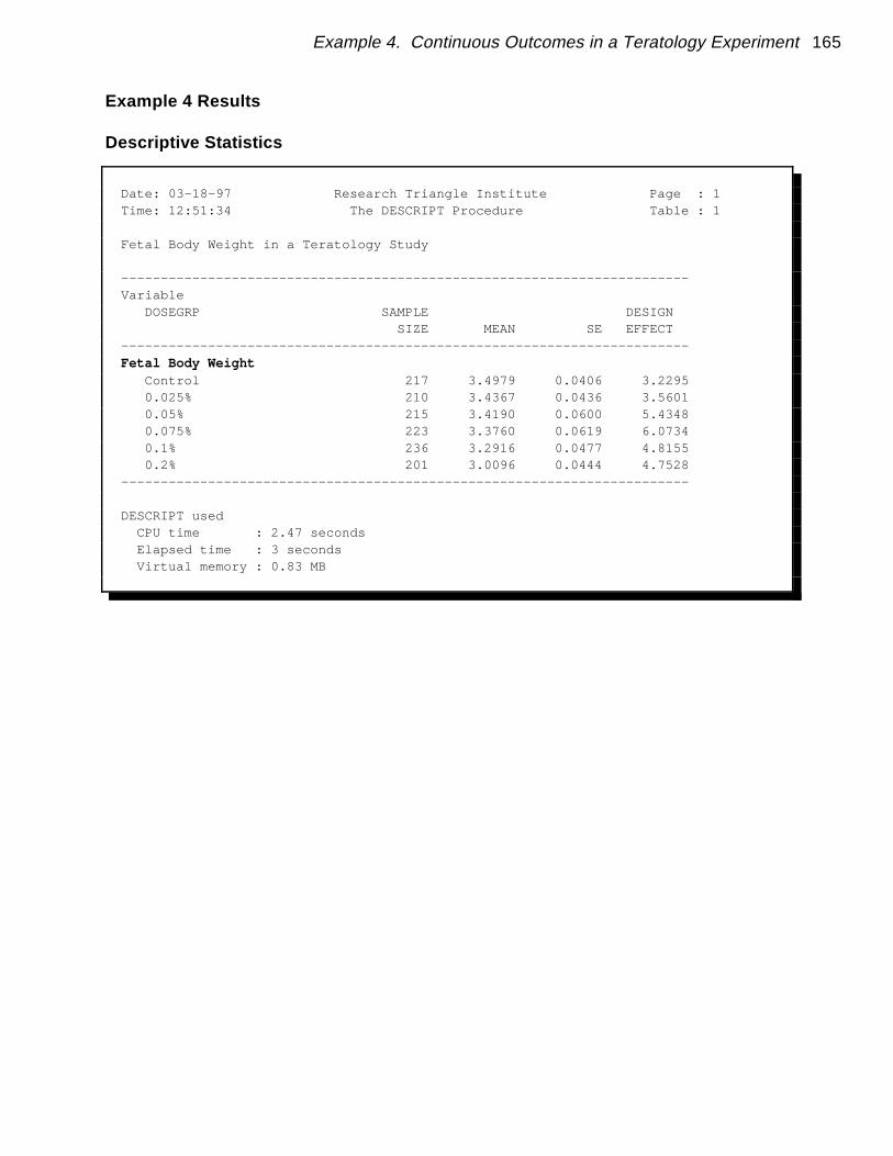
Example 4. Continuous Outcomes in a Teratology Experiment 165
Example 4 Results
Descriptive Statistics
Date: 03-18-97 Research Triangle Institute Page : 1 Time: 12:51:34 The DESCRIPT Procedure Table : 1
Fetal Body Weight in a Teratology Study
------------------------------------------------------------------------ Variable DOSEGRP SAMPLE DESIGN SIZE MEAN SE EFFECT ------------------------------------------------------------------------ Fetal Body Weight Control 217 3.4979 0.0406 3.2295 0.025% 210 3.4367 0.0436 3.5601 0.05% 215 3.4190 0.0600 5.4348 0.075% 223 3.3760 0.0619 6.0734 0.1% 236 3.2916 0.0477 4.8155 0.2% 201 3.0096 0.0444 4.7528 ------------------------------------------------------------------------
DESCRIPT used CPU time : 2.47 seconds Elapsed time : 3 seconds Virtual memory : 0.83 MB

166 SUDAAN Applications
Example 4 Results:
Regression ModellingThis first REGRESS procedure fits a linear regression model to the fetal body weights, withdose group (6-level categorical variable, from 1=control to 6=high dose) as the only predictor. We use the REFLEVEL statement to change the reference level for DOSEGRP from the defaultlast level (high dose) to the first (control). Now the regression parameters will be comparingeach treatment group to the control. We specify R=INDEPENDENT to estimate the model viaGEE under independent “working” correlations. The DAMID variable remains as the cluster onthe NEST statement. We also request the “Least Squares Means” for DOSEGRP. In this case,the least squares means will be equal to the raw means in each dose group, since DOSEGRP isthe only covariate in the model. SUDAAN notifies the user that there are 164 clusters, 1302fetuses (records on the file), and a min and max cluster size of 2 and 14, respectively.
10 PROC REGRESS DATA="c:\\tera\\examples\\boric" FILETYPE=SAS R=INDEPENDENT;
11 NEST _ONE_ DAMID;
12 WEIGHT _ONE_;
13 REFLEVEL DOSEGRP = 1;
14 SUBGROUP DOSEGRP;
15 LEVELS 6;
16 MODEL BW = DOSEGRP;
17 LSMEANS DOSEGRP;
18 SETENV COLSPCE=1 LABWIDTH=25 COLWIDTH=8 DECWIDTH=4 LINESIZE=78 PAGESIZE=60;
19 PRINT BETA="BETA" SEBETA="S.E." DEFT="DESIGN EFFECT" T_BETA="T:BETA=0" P_BETA="P-VALUE" DF WALDCHI WALDCHP / LSMEANS=ALL T_BETAFMT=F8.2 DEFTFMT=F6.2 DFFMT=F8.0 WALDCHIFMT=F8.2;
20 TITLE " " "Treatment Effect on Fetal Body Weight in a Teratology Experiment";
Opened SAS data file c:\tera\examples\boric.SSD for reading. Number of observations read : 1302 Weighted count: 1302 Observations used in the analysis : 1302 Weighted count: 1302 Observations with missing values : 0 Weighted count: 0 Denominator degrees of freedom : 163
Maximum number of estimable parameters for the model is 6
File c:\tera\examples\boric.SSD contains 164 clusters Maximum cluster size is 14 records Minimum cluster size is 2 records Weighted mean response is 3.341329
Multiple R-Square for the dependent variable BW: 0.171089
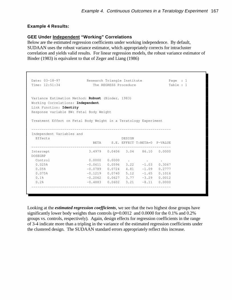
Example 4. Continuous Outcomes in a Teratology Experiment 167
Example 4 Results:
GEE Under Independent “Working” CorrelationsBelow are the estimated regression coefficients under working independence. By default,SUDAAN uses the robust variance estimator, which appropriately corrects for intraclustercorrelation and yields valid results. For linear regression models, the robust variance estimator ofBinder (1983) is equivalent to that of Zeger and Liang (1986)
Date: 03-18-97 Research Triangle Institute Page : 1 Time: 12:51:34 The REGRESS Procedure Table : 1
Variance Estimation Method: Robust (Binder, 1983)
Working Correlations: Independent Link Function: Identity Response variable BW: Fetal Body Weight
Treatment Effect on Fetal Body Weight in a Teratology Experiment
-------------------------------------------------------------------- Independent Variables and Effects DESIGN BETA S.E. EFFECT T:BETA=0 P-VALUE -------------------------------------------------------------------- Intercept 3.4979 0.0406 3.04 86.10 0.0000 DOSEGRP Control 0.0000 0.0000 . . . 0.025% -0.0611 0.0596 3.22 -1.03 0.3067 0.05% -0.0789 0.0724 4.81 -1.09 0.2777 0.075% -0.1219 0.0740 5.12 -1.65 0.1016 0.1% -0.2062 0.0627 3.77 -3.29 0.0012 0.2% -0.4883 0.0602 3.21 -8.11 0.0000
--------------------------------------------------------------------
Looking at the estimated regression coefficients, we see that the two highest dose groups havesignificantly lower body weights than controls (p=0.0012 and 0.0000 for the 0.1% and 0.2%groups vs. controls, respectively). Again, design effects for regression coefficients in the rangeof 3-4 indicate more than a tripling in the variance of the estimated regression coefficients underthe clustered design. The SUDAAN standard errors appropriately reflect this increase.

168 SUDAAN Applications
Example 4 Results:
GEE Under Independent “Working” Correlations
Date: 03-18-97 Research Triangle Institute Page : 2 Time: 12:51:34 The REGRESS Procedure Table : 1
Variance Estimation Method: Robust (Binder, 1983)
Working Correlations: Independent Link Function: Identity Response variable BW: Fetal Body Weight
Treatment Effect on Fetal Body Weight in a Teratology Experiment
---------------------------------------------------- Contrast Degrees P-value of Wald Wald Freedom ChiSq ChiSq ---------------------------------------------------- OVERALL MODEL 6 29189.67 0.0000 MODEL MINUS INTERCEPT 5 78.38 0.0000 INTERCEPT . . . DOSEGRP 5 78.38 0.0000
----------------------------------------------------
The main effects tests indicate that the overall effect of treatment (with 5 degrees of freedom) isstatistically significant, after adjusting for clustering (p=0.0000).

Example 4. Continuous Outcomes in a Teratology Experiment 169
Example 4 Results:
GEE Under Independent “Working” Correlations
Date: 03-18-97 Research Triangle Institute Page : 3 Time: 12:51:34 The REGRESS Procedure Table : 1
Variance Estimation Method: Robust (Binder, 1983)
Working Correlations: Independent Link Function: Identity Response variable BW: Fetal Body Weight
Treatment Effect on Fetal Body Weight in a Teratology Experiment
------------------------------------------------------------- Least-Square Means P-value SE LS T-Test T-Test LS Mean Mean LSM=0 LSM=0 ------------------------------------------------------------- DOSEGRP Control 3.4979 0.0406 86.1031 0.0000 0.025% 3.4367 0.0436 78.7976 0.0000 0.05% 3.4190 0.0600 57.0111 0.0000 0.075% 3.3760 0.0619 54.5351 0.0000 0.1% 3.2916 0.0477 68.9535 0.0000 0.2% 3.0096 0.0444 67.7343 0.0000 -------------------------------------------------------------
REGRESS used CPU time : 7.91 seconds Elapsed time : 8 seconds
Virtual memory : 1.29 MB
These Least-Squares Means are identical to the raw means and standard errors presented earlier,since there is only one covariate in the model. Body weights are reduced in the two highest dosegroups vs. controls. The standard errors of the least-squares means are adjusted for clustering.
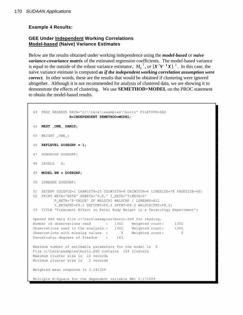
M 10 [X ��V 1X ]1
170 SUDAAN Applications
Example 4 Results:
GEE Under Independent Working Correlations Model-based (Naive) Variance Estimates
Below are the results obtained under working independence using the model-based or naivevariance-covariance matrix of the estimated regression coefficients. The model-based varianceis equal to the outside of the robust variance estimator, , or . In this case, thenaive variance estimate is computed as if the independent working correlation assumption werecorrect. In other words, these are the results that would be obtained if clustering were ignoredaltogether. Although it is not recommended for analysis of clustered data, we are showing it todemonstrate the effects of clustering. We use SEMETHOD=MODEL on the PROC statementto obtain the model-based results.
43 PROC REGRESS DATA="c:\\tera\\examples\\boric" FILETYPE=SAS R=INDEPENDENT SEMETHOD=MODEL;
44 NEST _ONE_ DAMID;
45 WEIGHT _ONE_;
46 REFLEVEL DOSEGRP = 1;
47 SUBGROUP DOSEGRP;
48 LEVELS 6;
49 MODEL BW = DOSEGRP;
50 LSMEANS DOSEGRP;
51 SETENV COLSPCE=1 LABWIDTH=25 COLWIDTH=8 DECWIDTH=4 LINESIZE=78 PAGESIZE=60; 52 PRINT BETA="BETA" SEBETA="S.E." T_BETA="T:BETA=0" P_BETA="P-VALUE" DF WALDCHI WALDCHP / LSMEANS=ALL T_BETAFMT=F8.2 DEFTFMT=F6.2 DFFMT=F8.0 WALDCHIFMT=F8.2; 53 TITLE “Treatment Effect on Fetal Body Weight in a Teratology Experiment";
Opened SAS data file c:\tera\examples\boric.SSD for reading. Number of observations read : 1302 Weighted count: 1302 Observations used in the analysis : 1302 Weighted count: 1302 Observations with missing values : 0 Weighted count: 0 Denominator degrees of freedom : 163
Maximum number of estimable parameters for the model is 6 File c:\tera\examples\boric.SSD contains 164 clusters Maximum cluster size is 14 records Minimum cluster size is 2 records
Weighted mean response is 3.341329
Multiple R-Square for the dependent variable BW: 0.171089

Example 4. Continuous Outcomes in a Teratology Experiment 171
Example 4 Results:
GEE Under Independent Working Correlations Model-based (Naive) Variance Estimates
Date: 03-18-97 Research Triangle Institute Page : 1 Time: 12:51:34 The REGRESS Procedure Table : 1
Variance Estimation Method: Model-Based (Naive) Working Correlations: Independent Link Function: Identity Response variable BW: Fetal Body Weight
Treatment Effect on Fetal Body Weight in a Teratology Experiment
-------------------------------------------------------------- Independent Variables and Effects BETA S.E. T:BETA=0 P-VALUE -------------------------------------------------------------- Intercept 3.4979 0.0233 150.15 0.0000 DOSEGRP Control 0.0000 0.0000 . . 0.025% -0.0611 0.0332 -1.84 0.0676 0.05% -0.0789 0.0330 -2.39 0.0180 0.075% -0.1219 0.0327 -3.73 0.0003 0.1% -0.2062 0.0323 -6.39 0.0000 0.2% -0.4883 0.0336 -14.54 0.0000 --------------------------------------------------------------
Here we see the estimated standard errors using the model-based approach under independenceare much smaller than with the robust variance estimator, with several of the lower dose groupsappearing significantly different from control. These estimates are overly optimistic (naive),computed as if the data were truely independent. Therefore, these results are not valid for thedata at hand. They merely demonstrate the consequences of ignoring the experimental design.

172 SUDAAN Applications
Example 4 Results:
GEE Under Independent Working Correlations Model-based (Naive) Variance Estimates
Date: 03-18-97 Research Triangle Institute Page : 2 Time: 12:51:34 The REGRESS Procedure Table : 1
Variance Estimation Method: Model-Based (Naive) Working Correlations: Independent Link Function: Identity Response variable BW: Fetal Body Weight
Treatment Effect on Fetal Body Weight in a Teratology Experiment
---------------------------------------------------- Contrast Degrees P-value of Wald Wald Freedom ChiSq ChiSq ---------------------------------------------------- OVERALL MODEL 6 ******** 0.0000 MODEL MINUS INTERCEPT 5 267.50 0.0000 INTERCEPT . . . DOSEGRP 5 267.50 0.0000 ----------------------------------------------------
This table contains the main effects tests assuming the naive assumption of independence weretrue. The p-value according to the treatment effect is still significant (p=0.0000), but the Waldchi-square is much larger (267.5) than under the robust variance approach.

Example 4. Continuous Outcomes in a Teratology Experiment 173
Example 4 Results:
GEE Under Independent Working Correlations Model-based (Naive) Variance Estimates
Date: 03-18-97 Research Triangle Institute Page : 3 Time: 12:51:34 The REGRESS Procedure Table : 1
Variance Estimation Method: Model-Based (Naive)
Working Correlations: Independent Link Function: Identity Response variable BW: Fetal Body Weight
Treatment Effect on Fetal Body Weight in a Teratology Experiment
------------------------------------------------------------- Least-Square Means P-value SE LS T-Test T-Test LS Mean Mean LSM=0 LSM=0 ------------------------------------------------------------- DOSEGRP Control 3.4979 0.0233 150.1543 0.0000 0.025% 3.4367 0.0237 145.1315 0.0000 0.05% 3.4190 0.0234 146.0900 0.0000 0.075% 3.3760 0.0230 146.9116 0.0000 0.1% 3.2916 0.0223 147.3570 0.0000 0.2% 3.0096 0.0242 124.3387 0.0000 -------------------------------------------------------------
REGRESS used CPU time : 7.9 seconds Elapsed time : 8 seconds Virtual memory : 1.29 MB
Under the model-based approach, the Least Squares Means are the same as before, but theirestimated standard errors are misleadingly small, computed as if the independence assumptionwere true.

174 SUDAAN Applications
Example 4 Results:
GEE under Exchangeable Working Correlations
Below are the programming statements to estimate the linear model under exchangeableworking correlations. The only change from the previous statements is the switch fromR=INDEPENDENT to R=EXCHANGE on the PROC statement. All other statements remainunchanged. By default, SUDAAN will use the GEE 1-step approach for estimating regressionparameters, with the independence parameter estimates being updated exactly once with theestimated correlation structure. SUDAAN notifies the user that there are 164 clusters, 1302fetuses, and a min and max cluster size of 2 and 14, respectively. Below is the first page of theREGRESS procedure output:
21 PROC REGRESS DATA="c:\\tera\\examples\\boric" FILETYPE=SAS R=EXCHANGE;
22 NEST _ONE_ DAMID;
23 WEIGHT _ONE_;
24 REFLEVEL DOSEGRP = 1;
25 SUBGROUP DOSEGRP;
26 LEVELS 6;
27 MODEL BW = DOSEGRP;
28 LSMEANS DOSEGRP;
29 SETENV COLSPCE=1 LABWIDTH=25 COLWIDTH=8 DECWIDTH=4 LINESIZE=78 PAGESIZE=60;
30 PRINT BETA="BETA" SEBETA="S.E." DEFT="DESIGN EFFECT" T_BETA="T:BETA=0" P_BETA="P-VALUE" DF WALDCHI WALDCHP / LSMEANS=ALL RHOS=ALL T_BETAFMT=F8.2 DEFTFMT=F6.2 DFFMT=F8.0 WALDCHIFMT=F8.2;
31 TITLE " " "Treatment Effect on Fetal Body Weight in a Teratology Experiment";
Opened SAS data file c:\tera\examples\boric.SSD for reading. Number of observations read : 1302 Weighted count: 1302 Observations used in the analysis : 1302 Weighted count: 1302 Observations with missing values : 0 Weighted count: 0 Denominator degrees of freedom : 163
Maximum number of estimable parameters for the model is 6
File c:\tera\examples\boric.SSD contains 164 clusters Maximum cluster size is 14 records Minimum cluster size is 2 records Weighted mean response is 3.341329
Multiple R-Square for the dependent variable BW: 0.169118

Example 4. Continuous Outcomes in a Teratology Experiment 175
Example 4 Results:
GEE Under Exchangeable Working Correlations
Date: 03-18-97 Research Triangle Institute Page : 3 Time: 12:51:34 The REGRESS Procedure Table : 1
Variance Estimation Method: Robust (Binder, 1983)
Working Correlations: Exchangeable Link Function: Identity Response variable BW: Fetal Body Weight
Treatment Effect on Fetal Body Weight in a Teratology Experiment
---------------------------------- Variable Correlation Matrix ---------------------------------- Fetal Body Weight 0.5056
----------------------------------
The estimated exchangeable correlation parameter (measure of pairwise dependence withinclusters) is 0.5056. The relatively large size of the intracluster correlation is partly responsiblefor the large design effects (variance inflation) for estimated means and regression parametersseen already. Variance inflation is directly related to the size of the intracluster correlation andthe average cluster size (here, number of fetuses per litter).

176 SUDAAN Applications
Example 4 Results:
GEE Under Exchangeable Working Correlations
Date: 03-18-97 Research Triangle Institute Page : 1 Time: 12:51:34 The REGRESS Procedure Table : 1
Variance Estimation Method: Robust (Binder, 1983)
Working Correlations: Exchangeable Link Function: Identity Response variable BW: Fetal Body Weight
Treatment Effect on Fetal Body Weight in a Teratology Experiment
-------------------------------------------------------------- Independent Variables and Effects BETA S.E. T:BETA=0 P-VALUE -------------------------------------------------------------- Intercept 3.5125 0.0470 74.67 0.0000 DOSEGRP Control 0.0000 0.0000 . . 0.025% -0.0509 0.0622 -0.82 0.4148 0.05% -0.0656 0.0738 -0.89 0.3753 0.075% -0.1363 0.0790 -1.73 0.0864 0.1% -0.2409 0.0680 -3.54 0.0005 0.2% -0.4822 0.0651 -7.40 0.0000
--------------------------------------------------------------
Above are the estimated regression coefficients under exchangeability, with a robust varianceestimator. We see that these results are qualitatively the same as “working” independenceshowed previously. Modelling the within-cluster covariance structure has not improvedefficiency in these data.
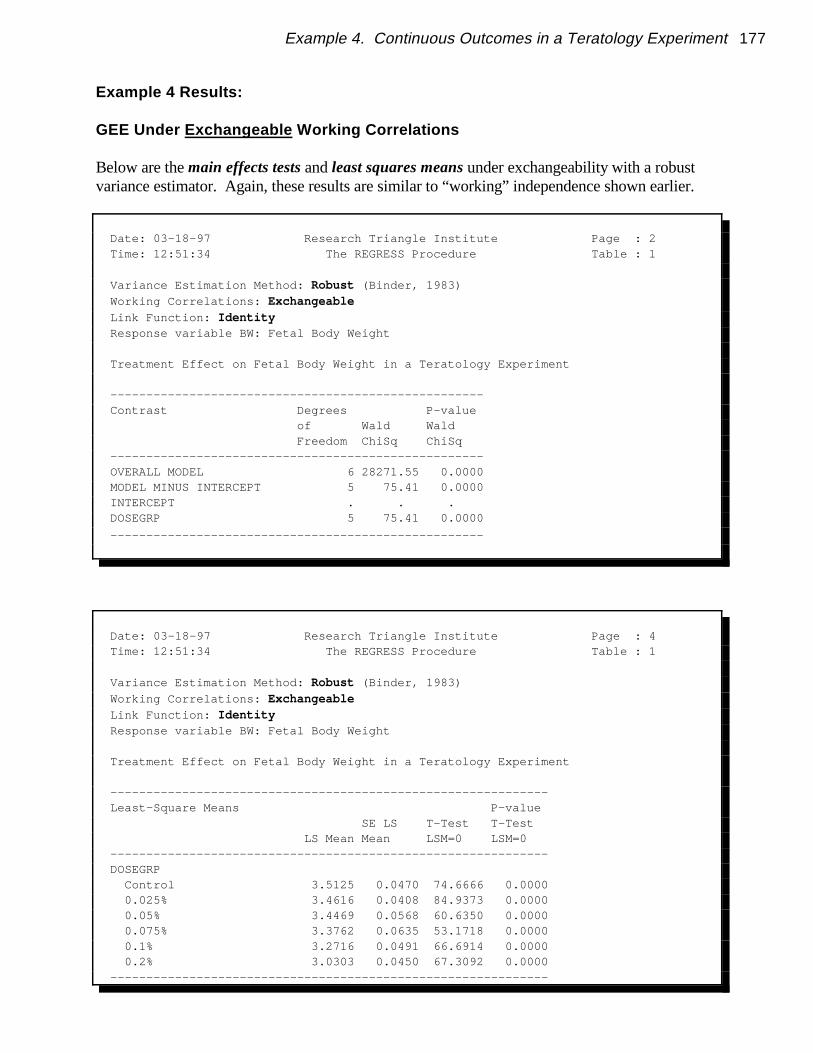
Example 4. Continuous Outcomes in a Teratology Experiment 177
Example 4 Results:
GEE Under Exchangeable Working Correlations
Below are the main effects tests and least squares means under exchangeability with a robustvariance estimator. Again, these results are similar to “working” independence shown earlier.
Date: 03-18-97 Research Triangle Institute Page : 2 Time: 12:51:34 The REGRESS Procedure Table : 1
Variance Estimation Method: Robust (Binder, 1983)
Working Correlations: Exchangeable Link Function: Identity Response variable BW: Fetal Body Weight
Treatment Effect on Fetal Body Weight in a Teratology Experiment
---------------------------------------------------- Contrast Degrees P-value of Wald Wald Freedom ChiSq ChiSq ---------------------------------------------------- OVERALL MODEL 6 28271.55 0.0000 MODEL MINUS INTERCEPT 5 75.41 0.0000 INTERCEPT . . . DOSEGRP 5 75.41 0.0000
----------------------------------------------------
Date: 03-18-97 Research Triangle Institute Page : 4 Time: 12:51:34 The REGRESS Procedure Table : 1
Variance Estimation Method: Robust (Binder, 1983)
Working Correlations: Exchangeable Link Function: Identity Response variable BW: Fetal Body Weight
Treatment Effect on Fetal Body Weight in a Teratology Experiment
------------------------------------------------------------- Least-Square Means P-value SE LS T-Test T-Test LS Mean Mean LSM=0 LSM=0 ------------------------------------------------------------- DOSEGRP Control 3.5125 0.0470 74.6666 0.0000 0.025% 3.4616 0.0408 84.9373 0.0000 0.05% 3.4469 0.0568 60.6350 0.0000 0.075% 3.3762 0.0635 53.1718 0.0000 0.1% 3.2716 0.0491 66.6914 0.0000 0.2% 3.0303 0.0450 67.3092 0.0000 -------------------------------------------------------------
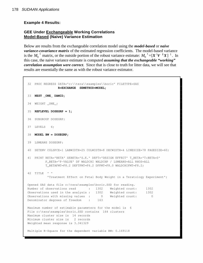
M 10 M 1
0 [X ��V 1X ]1
178 SUDAAN Applications
Example 4 Results:
GEE Under Exchangeable Working CorrelationsModel-Based (Naive) Variance Estimation
Below are results from the exchangeable correlation model using the model-based or naivevariance-covariance matrix of the estimated regression coefficients. The model-based varianceis the matrix, or the outside portion of the robust variance estimate: = . Inthis case, the naive variance estimate is computed assuming that the exchangeable “working”correlation assumption were correct. Since that is close to truth for litter data, we will see thatresults are essentially the same as with the robust variance estimator.
32 PROC REGRESS DATA="c:\\tera\\examples\\boric" FILETYPE=SAS R=EXCHANGE SEMETHOD=MODEL;
33 NEST _ONE_ DAMID;
34 WEIGHT _ONE_;
35 REFLEVEL DOSEGRP = 1;
36 SUBGROUP DOSEGRP;
37 LEVELS 6;
38 MODEL BW = DOSEGRP;
39 LSMEANS DOSEGRP;
40 SETENV COLSPCE=1 LABWIDTH=25 COLWIDTH=8 DECWIDTH=4 LINESIZE=78 PAGESIZE=60;
41 PRINT BETA="BETA" SEBETA="S.E." DEFT="DESIGN EFFECT" T_BETA="T:BETA=0" P_BETA="P-VALUE" DF WALDCHI WALDCHP / LSMEANS=ALL RHOS=ALL T_BETAFMT=F8.2 DEFTFMT=F6.2 DFFMT=F8.0 WALDCHIFMT=F8.2;
42 TITLE " " "Treatment Effect on Fetal Body Weight in a Teratology Experiment";
Opened SAS data file c:\tera\examples\boric.SSD for reading. Number of observations read : 1302 Weighted count: 1302 Observations used in the analysis : 1302 Weighted count: 1302 Observations with missing values : 0 Weighted count: 0 Denominator degrees of freedom : 163
Maximum number of estimable parameters for the model is 6 File c:\tera\examples\boric.SSD contains 164 clusters Maximum cluster size is 14 records Minimum cluster size is 2 records Weighted mean response is 3.341329
Multiple R-Square for the dependent variable BW: 0.169118

Example 4. Continuous Outcomes in a Teratology Experiment 179
Example 4 Results:
GEE Under Exchangeable Working CorrelationsModel-Based (Naive) Variance Estimation
Date: 03-18-97 Research Triangle Institute Page : 1 Time: 12:51:34 The REGRESS Procedure Table : 1
Variance Estimation Method: Model-Based (Naive) Working Correlations: Exchangeable Link Function: Identity Response variable BW: Fetal Body Weight
Treatment Effect on Fetal Body Weight in a Teratology Experiment
-------------------------------------------------------------- Independent Variables and Effects BETA S.E. T:BETA=0 P-VALUE -------------------------------------------------------------- Intercept 3.5125 0.0519 67.69 0.0000 DOSEGRP Control 0.0000 0.0000 . . 0.025% -0.0509 0.0719 -0.71 0.4799 0.05% -0.0656 0.0730 -0.90 0.3701 0.075% -0.1363 0.0723 -1.88 0.0613 0.1% -0.2409 0.0721 -3.34 0.0010 0.2% -0.4822 0.0737 -6.54 0.0000 ---------------------------------------------------------------
Here we have the estimated regression coefficients computed under exchangeability and thestandard errors as if the exchangeable working asssumption were correct. The standard errors areroughly the same as with the robust variance estimator for these data, indicating that theexchangeable correlation assumption is close to truth.

180 SUDAAN Applications
Example 4 Results:
GEE Under Exchangeable Working CorrelationsModel-Based (Naive) Variance Estimation
Date: 03-18-97 Research Triangle Institute Page : 2 Time: 12:51:34 The REGRESS Procedure Table : 1
Variance Estimation Method: Model-Based (Naive) Working Correlations: Exchangeable Link Function: Identity Response variable BW: Fetal Body Weight
Treatment Effect on Fetal Body Weight in a Teratology Experiment
---------------------------------------------------- Contrast Degrees P-value of Wald Wald Freedom ChiSq ChiSq ---------------------------------------------------- OVERALL MODEL 6 26050.93 0.0000 MODEL MINUS INTERCEPT 5 58.46 0.0000 INTERCEPT . . . DOSEGRP 5 58.46 0.0000 ----------------------------------------------------
Here we have the main effects tests computed under exchangeability, using the model-basedvariance approach. Results are essentially the same as with the robust variance estimator.

Example 4. Continuous Outcomes in a Teratology Experiment 181
Example 4 Results:
GEE Under Exchangeable Working CorrelationsModel-Based (Naive) Variance Estimation
Date: 03-18-97 Research Triangle Institute Page : 4 Time: 12:51:34 The REGRESS Procedure Table : 1
Variance Estimation Method: Model-Based (Naive) Working Correlations: Exchangeable Link Function: Identity Response variable BW: Fetal Body Weight
Treatment Effect on Fetal Body Weight in a Teratology Experiment
------------------------------------------------------------- Least-Square Means P-value SE LS T-Test T-Test LS Mean Mean LSM=0 LSM=0 ------------------------------------------------------------- DOSEGRP Control 3.5125 0.0519 67.6924 0.0000 0.025% 3.4616 0.0497 69.6389 0.0000 0.05% 3.4469 0.0513 67.1676 0.0000 0.075% 3.3762 0.0504 66.9663 0.0000 0.1% 3.2716 0.0501 65.3301 0.0000 0.2% 3.0303 0.0523 57.9232 0.0000 -------------------------------------------------------------
REGRESS used CPU time : 7.19 seconds Elapsed time : 8 seconds Virtual memory : 1.34 MB

182 SUDAAN Applications
Example 4 Results:
Jackknife Variance EstimationBelow are the modelling results using an alternative approach: Jackknife variance estimation. We obtained these results by specifying DESIGN=JACKKNIFE on the PROC statement.
54 PROC REGRESS DATA="c:\\tera\\examples\\boric" FILETYPE=SAS DESIGN=JACKKNIFE;
55 NEST _ONE_ DAMID;
56 WEIGHT _ONE_;
57 REFLEVEL DOSEGRP = 1;
58 SUBGROUP DOSEGRP;
59 LEVELS 6;
60 MODEL BW = DOSEGRP;
61 LSMEANS DOSEGRP;
62 SETENV COLSPCE=1 LABWIDTH=25 COLWIDTH=8 DECWIDTH=4 LINESIZE=78 PAGESIZE=60;
63 PRINT BETA="BETA" SEBETA="S.E." DEFT="DESIGN EFFECT" T_BETA="T:BETA=0" P_BETA="P-VALUE" DF WALDCHI WALDCHP / LSMEANS=ALL T_BETAFMT=F8.2 DEFTFMT=F6.2 DFFMT=F8.0 WALDCHIFMT=F8.2;
64 TITLE " " "Treatment Effect on Fetal Body Weight in a Teratology Experiment";
Opened SAS data file c:\tera\examples\boric.SSD for reading.
Number of observations read : 1302 Weighted count: 1302 Observations used in the analysis : 1302 Weighted count: 1302 Observations with missing values : 0 Weighted count: 0 Denominator degrees of freedom : 163
Maximum number of estimable parameters for the model is 6 File c:\tera\examples\boric.SSD contains 164 clusters Maximum cluster size is 14 records Minimum cluster size is 2 records Weighted mean response is 3.341329
Multiple R-Square for the dependent variable BW: 0.171089

Example 4. Continuous Outcomes in a Teratology Experiment 183
Example 4 Results:
Jackknife Variance EstimationBelow are the estimated regression coefficients and standard errors under the Jackknife option. Note that the regression coefficients are simply those computed under independence. Theestimated standard errors are computed using the Jackknife variance estimator. Note the resultsfor this example are similar to those obtained under GEE-independent and GEE-exchangeable.
Date: 03-18-97 Research Triangle Institute Page : 1 Time: 12:51:34 The REGRESS Procedure Table : 1
Variance Estimation Method: Jackknife Working Correlations: Independent Link Function: Identity Response variable BW: Fetal Body Weight
Treatment Effect on Fetal Body Weight in a Teratology Experiment
-------------------------------------------------------------------- Independent Variables and Effects DESIGN BETA S.E. EFFECT T:BETA=0 P-VALUE -------------------------------------------------------------------- Intercept 3.4979 0.0419 3.23 83.52 0.0000 DOSEGRP Control 0.0000 0.0000 . . . 0.025% -0.0611 0.0616 3.44 -0.99 0.3227 0.05% -0.0789 0.0752 5.18 -1.05 0.2955 0.075% -0.1219 0.0765 5.46 -1.59 0.1128 0.1% -0.2062 0.0648 4.03 -3.18 0.0018 0.2% -0.4883 0.0624 3.45 -7.83 0.0000 --------------------------------------------------------------------
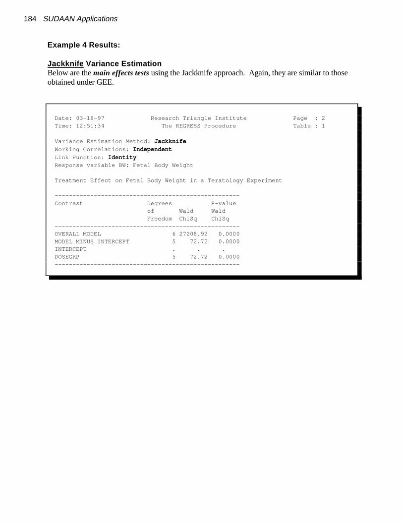
184 SUDAAN Applications
Example 4 Results:
Jackknife Variance EstimationBelow are the main effects tests using the Jackknife approach. Again, they are similar to thoseobtained under GEE.
Date: 03-18-97 Research Triangle Institute Page : 2 Time: 12:51:34 The REGRESS Procedure Table : 1
Variance Estimation Method: Jackknife Working Correlations: Independent Link Function: Identity Response variable BW: Fetal Body Weight
Treatment Effect on Fetal Body Weight in a Teratology Experiment
---------------------------------------------------- Contrast Degrees P-value of Wald Wald Freedom ChiSq ChiSq ---------------------------------------------------- OVERALL MODEL 6 27208.92 0.0000 MODEL MINUS INTERCEPT 5 72.72 0.0000 INTERCEPT . . . DOSEGRP 5 72.72 0.0000 ----------------------------------------------------
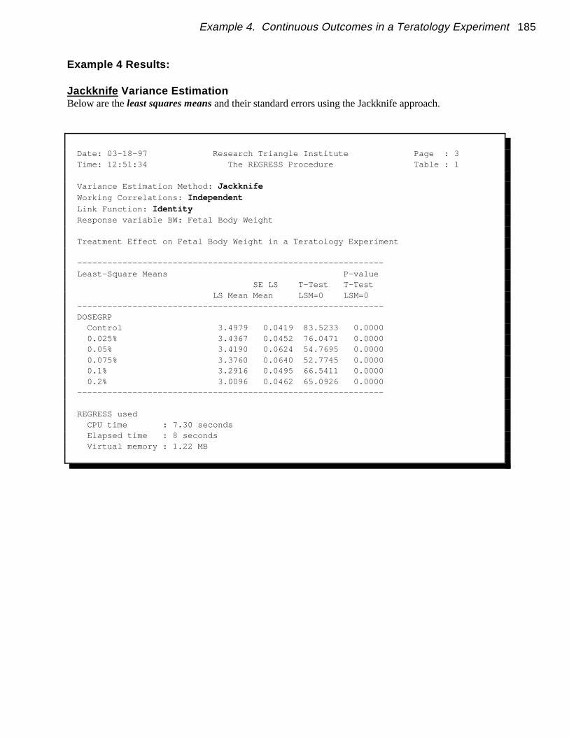
Example 4. Continuous Outcomes in a Teratology Experiment 185
Example 4 Results:
Jackknife Variance EstimationBelow are the least squares means and their standard errors using the Jackknife approach.
Date: 03-18-97 Research Triangle Institute Page : 3 Time: 12:51:34 The REGRESS Procedure Table : 1
Variance Estimation Method: Jackknife Working Correlations: Independent Link Function: Identity Response variable BW: Fetal Body Weight
Treatment Effect on Fetal Body Weight in a Teratology Experiment
------------------------------------------------------------- Least-Square Means P-value SE LS T-Test T-Test LS Mean Mean LSM=0 LSM=0 ------------------------------------------------------------- DOSEGRP Control 3.4979 0.0419 83.5233 0.0000 0.025% 3.4367 0.0452 76.0471 0.0000 0.05% 3.4190 0.0624 54.7695 0.0000 0.075% 3.3760 0.0640 52.7745 0.0000 0.1% 3.2916 0.0495 66.5411 0.0000 0.2% 3.0096 0.0462 65.0926 0.0000 -------------------------------------------------------------
REGRESS used CPU time : 7.30 seconds Elapsed time : 8 seconds Virtual memory : 1.22 MB

186 SUDAAN Applications

Appendix III:
Comparisons to Other Methods

188 SUDAAN Applications
Modelling vs. Accounting for Correlation
EFFICIENCY
Cluster-level or Time-stationary covariates:That is, a covariate that takes on the same value for all members of agiven cluster (i.e., constant within a cluster)
e.g., a common treatment applied to all members of a givencluster.
Modelling the correlation structure and accounting for intraclustercorrelation have similar efficiency and power to detect cluster-levelcovariate effects.
References: Bieler and Williams, 1994Neuhaus, 1993Lipsitz, et al., 1994a, 1994bMancl and Leroux, 1996
APPENDIX III: Comparisons to Other Methods 189
Modelling vs. Accounting for Correlation
EFFICIENCY
Within-Cluster or Time-Varying Covariates:A covariate where each member of a given cluster can potentially takeon its own value (i.e., not constant within a cluster)
Modelling the intracluster correlation:
� Provides more efficient estimation and more powerful tests ofwithin-cluster covariates with different covariate patterns acrossindividuals:
e.g., Smoking Status at various points in time
Gains in efficiency increase with response intracluster correlation
� Provides no increase in efficiency for within-cluster covariates inwhich the pattern of the within-cluster covariate is the same for allclusters (for example, covariates that can be experimentallymanipulated):
e.g., the effect of time, where time may be recorded as theoccasions of measurement (1, 2, 3, 4) for each individual
References: Neuhaus, 1993Lipsitz, et al., 1994a, 1994bMancl and Leroux, 1996

190 SUDAAN Applications
Other Comparisons
GEE / SUDAAN: Comparisons to other procedures andpackages:
Vs. SAS PROC MIXED and BMDP5V:
� Same idea (Population-averaged or "marginal" models), and sameestimating equations IF you specify only fixed effects and supply anassumed correlation structure for the random errors;
� Mixed models in SAS also allow for random effects (which aresometimes called cluster-specific models, because individual clusterdeviations from population-averaged intercepts and slopes can beestimated); SUDAAN and the GEE macro of Karim and Zeger (1989)do not allow for random effects; this area is developing!
� Continuous outcomes only; use maximum likelihood (or REML) undera multivariate normality assumption to estimate � and Vi
� SAS produces the naive or model-based variance estimate, and recentlythe robust variance estimator. The model-based variance assumes theworking correlation structure is correct. Most important if you specify"independent" working correlations!
� SAS does not iterate between correlations and regression coefficients; itestimates V directlyi
Biomedical Research:Laird and Ware (1982); Laird, et al (1992)
Psychology and Behavioral Research:Bryk and Raudenbush (1987)Goldstein (1987)Hedeker, Gibbons, and Davis (1991)Hedeker, Gibbons, and Flay (1994)

y X� � Zv � �
Ev
�
0
0
Varv
�
G 0
0 R
V(y) ZGZ ��� R
)2
v
APPENDIX III: Comparisons to Other Methods 191
Other Comparisons
Review of the General Linear Mixed Model
� Extension of the General Linear Model by allowing both correlation andnon-identicality (heterogeneity of variance), although still assumingnormality:
� Elements of � not independent and identically distributed with zeromean and variance (however, normality still assumed).
� y is an observed data vectorX is the design matrix for the unknown fixed effects, ��
Z is a design matrix for the unknown random effects, � is a vector of unobserved random errors.

� (X ��V 1X ) X ��V 1y
Var(�) (X ��R1X )1 (M odelbased)
Z0 R )2I
192 SUDAAN Applications
Other Comparisons
Review of the General Linear Mixed Model (continued)
� Model V by setting up a random-effects design matrix Z and byspecifying covariance structures for G and R
For example, the General Linear Model is a special case of a mixedmodel with and
� Estimates of fixed effects parameters (ML or REML):
� Therefore, mixed models can be used for modelling repeated measuresor longitudinal data:
R matrix is the place to model the covariance structure of a subject'sdata: e.g., compound symmetry, AR(1), unstructured.
� Note that the estimating equations have the same form as GEE

APPENDIX III: Comparisons to Other Methods 193
Other Comparisons
GEE / SUDAAN: Comparisons to other procedures andpackages:
Vs. SAS GLM :
� Idea is that of MIXED with exchangeable correlations (if you use theunivariate approach) with fewer options for the correlation matrix (i.e.,fits the compound symmetry structure only).
� Throws out entire clusters with missing observations
� Method-of-moments estimation for variance components; least squaresfor parameter estimation
Vs. SAS CATMOD
� Log-linear modelling of contingency tables
� GSK and WLS methods See Koch, et al, 1977; Grizzle, Starmer, Koch, 1969
� Analogy: CATMOD : GEE as ANOVA : REGRESSIONi.e., good for categorical covariates that are not sparsely distributed
See Zeger, 1988
194 SUDAAN Applications
Other Comparisons
GEE / SUDAAN: Comparisons to other procedures andpackages:
Vs. Conditional Logistic Regression and Mixed Logistic Models
� Mixed effects models and random regression models for binary andordinal responses:
Stiratelli, Laird, and Ware (1984)Gibbons and Hedeker (1994)Hedeker and Gibbons (1994)
� Conditional likelihood approach for matched pair data:Breslow and Day (1980).
� Cluster-specific parameters in model; intercept terms allowed to varybetween clusters according to a specified distribution
� Regression coefficients have different meaning than for marginalmodels; tells how covariates effect responses for particular "latent" riskgroups represented by the random intercepts
� Random effects and mixed models better for within-cluster covariates
Comparisons more fully discussed in:
Neuhaus, Kalbfleisch, and Hauck, 1991Zeger, Liang, and Albert, 1988Park, 1993