Poser, Jason. 2012. Comparative Imagery Analysis of Non-Metric Cameras from Unmanned Aerial Survey

Aircraft. Volume 14, Papers in Resource Analysis. 20 pp. Saint Mary’s University of Minnesota Central

Services Press. Winona, MN. Retrieved (date) from http://www.gis.smumn.edu.

Comparative Imagery Analysis of Non-Metric Cameras from Unmanned Aerial Survey

Aircraft

Jason Poser

Department of Resource Analysis, Saint Mary’s University of Minnesota, Winona, Minnesota

55987

Keywords: GIS, UAS, UAV, Photogrammetry, DTM, GCP, Non-Metric, GSD, Orthomosaics

Abstract

Unmanned aerial survey imagery from non-metric cameras was analyzed for suitability,

stability, and resolution within a geographic information system. A powered parachute

aircraft was designed for the research and used to obtain imagery using two cameras. The

research implemented three commercial photogrammetry applications to assess and isolate

any application specific nuances that may affect the resulting datasets. Using Esri’s ArcMap,

a comparative analysis of the resulting orthomosaics and digital terrain models was

conducted. The findings of the research indicate that quality datasets obtained using the

methods described are plausible and realistic. Expectations of spatial accuracy and terrain

resolution were met.

Introduction

Aerial imaging started more than 150

years ago. According to the Professional

Aerial Photographers Association (2012),

aerial photography was first practiced by

French photographer and balloonist

Gaspard- Félix Tournachon (“Nadar”).

Unfortunately those early photographs no

longer survive. The oldest aerial

photograph known to exist is James

Wallace Black’s image of Boston in 1860.

It was not until World War I that

aerial photography made by aerial

observers replaced drawings and sketches

of the battlefields. By the end of the war

aerial photographs were recording the

entire front twice daily. At the end of the

war aerial cameras first transitioned to

non-military purposes when in 1921

Sherman Fairchild produced overlapping

photographs that made a map of

Manhattan Island (Professional Aerial

Photographers Association, 2012). This

aerial map was a commercial success and

used throughout New York City’s

administrative agencies and businesses.

With other cities following, aerial surveys

proved to be faster and less expensive than

traditional ground surveys.

Today, 91 years after Sherman

Fairchild made his Manhattan Island map,

with the advent and rapid adoption of web-

based consumer mapping products such as

Google Earth and Bing maps, the demand

and use for aerial imaging has become

common in consumer navigation and

mobile web-based location information

services. Aerial imagery has become a

common spatial background from which

other feature datasets are created. The

demand for ever increasing accuracy and

resolution for a lower cost and faster

delivery is the primary motivation for this

research. Advancements in camera

technology and the reduction in camera

costs have made it possible to obtain low-

cost ultrahigh resolution spatially accurate

2

imagery in a static environment.

In addition to advancements in

camera technology, advancements in flight

technology have also occurred including

the rise of the unmanned aerial vehicle

(UAV) industry. Rapid development of the

UAV industry can be largely credited to

military research and development during

the last decade. Companies such as

Boeing, Lockheed Martin, BAE, and

Northrop Grumman are changing the way

data are collected in theatres of conflict

across the globe and are influencing new

innovation commercially (Abramson,

2012).

The acceptance of civil market

UAV usage is rapidly approaching and

Congress, the FAA, and the nation are

questioning the role and scope in which

civil UAV use in commercial airspace will

be permitted, with safety and privacy

being the two highest concerns. This paper

will not focus on social and legal

implications of UAV use in the United

State’s airspace as these are serious and

complicated issues that need to be

considered before unmanned aircraft are

widely adopted.

The purpose of this paper is to

provide a methodology to validate imagery

derived from unmanned aerial vehicles for

use in civil geospatial projects. The

fundamental question is whether or not the

combination of digital aerial image sensors

coupled with unmanned aerial vehicles can

produce reliable, consistent, commercially

comparable datasets that represent as good

or better resolution for use in geographic

information system (GIS) centric mapping

as presently exists. For UAV-based aerial

imagery to be considered useful for this

project, it is important that UAV-derived

imagery be of a calculable quality

compared to that of traditional aerial

imagery products. The direction of this

research is to illustrate a GIS approach for

the analysis of UAV-derived spatially

accurate imagery.

An attempt was made in this

research to determine appreciable imagery

differences between two different sensors

on board a UAV aircraft. Current

commercial UAV systems are fully

capable of supporting a wide range of

digital sensors; however most of the

existing imaging systems currently used

are largely cost-prohibitive for the civil

market and small budget programs.

However, smaller boutique hobbyist grade

UAV systems are rapidly entering the

market with increased accuracy and lower

cost making unmanned aerial surveys

more feasible. These systems are largely

limited to supporting small consumer-

grade non-metric cameras typically

weighing less than 600g. This research

specifically evaluates the effectiveness of

non-metric cameras on board UAV aircraft

for use in aerial imaging.

Photogrammetry Software

Traditional aerial photogrammetry

workflows are developed to work in

conjunction with imagery captured from

precisely controlled piloted aircraft. The

unique nature and variability of unmanned

aerial vehicle surveys may present

challenges for existing aerial

photogrammetry software systems in how

they process the datasets. One component

of this research is to analyze and attempt

to isolate the relationship between the

inherent raw image accuracy and

processed image accuracy.

Non-metric Camera Geometric Stability

Imaging system performance depends on

several variables. In addition to the

camera’s sensor size, its lens system,

aperture, ISO capability, and frame rate

3

each contribute a unique set of

performance factors to the overall system

design. Metric and non-metric is one way

of classifying cameras used for obtaining

aerial imagery. Metric cameras are

constructed following strict criteria related

to internal camera dimensions. These

cameras are certified to perform

consistently from image capture to image

capture without variation in image

distortion. Non-metric cameras such as

most consumer-grade cameras are not

designed to meet these rigorous standards.

Often non-metric cameras have variable

zoom focus lenses which add yet another

level of uncertainly to the camera’s

stability over time.

A second component of the

research was to explore whether current

non-metric cameras provide for reasonably

consistent results in terms of geometric

stability for use in aerial survey. Can non-

metric point and shoot cameras of good to

excellent quality provide the geometric

stability that is traditionally required by

commercial aerial photogrammetry

software packages? Furthermore, it is

expected that measurable differences in

the camera calibration will occur over time

being that the lens system auto retracts

during each power cycle whereas fixed

focal length systems typically retain their

geometric stability regardless of the power

cycle. Previous data suggests non-metric

cameras can perform well in terms of

photogrammetric stability (Stahlke, 2011).

For this study, camera calibration results

before and after flight were used to

explore this question as well as the

performance of the photogrammetry

software with the input parameters from

the camera calibration.

Methods

Vehicle Platform

Three UAV aircrafts were designed and

fabricated for this research, while only one

aircraft was used for actual data collection

(Figures 1 and 2). In terms of time and

resources, the process of designing,

fabricating, and testing was by far the

most laborious component of this project.

To that degree, a firm understanding of

how the research aircraft impacts the

imagery needed to be explored and tested.

Figure 1. Powered parachute UAVs designed and

fabricated as part of the research.

Figure 2. Powered parachute UAV aircraft

designed and fabricated as part of the research.

Three distinct platforms were considered

for the research: fixed-wing aircraft, multi-

rotor helicopter, and a powered parachute.

Ultimately, the aircraft design series that

was chosen was designed around powered

parachutes. The criteria needed for the

platforms were:

4

1. Safety: The aircraft needed to be

able to prevent harm to the general

public and/or damage to the

calibrated cameras used in the

research.

2. Relatively slow airspeed to help

minimize motion image blur.

3. Large configurable payload

capability to host several sensor

configurations depending on the

data that needs to be collected.

The most suitable aircraft in terms

of technical abilities was a multi-rotor

helicopter. Multi-rotor helicopters offer

precise flight control with vertical lift and

landing capabilities that are ideal for small

area studies. The defining drawback to

these systems is the safety. The multi-rotor

helicopters use multiple precisely timed

motors, multiple motor controllers, and

multiple propellers to maintain stable

flight. Should any of these components

fail, the helicopter’s stability deteriorates

at an alarming rate and commonly results

in an uncontrolled free fall crash.

Powered parachutes were the most

suitable platform when the research

commenced. Powered parachutes fly

relatively slow using a ram airfoil

parachute. Lift is generated by the

parachute when the baffles of the

parachute are inflated; the inflated

parachute creates a wing surface like that

of a typical aircraft. In the unlikely event

of total electrical failure resulting in the

loss of navigation and propulsion, a

powered parachute would pose the least

risk to injury and property of the general

public.

Image Sensors

To test the question of geometric stability

of variable focus point-and-shoot

consumer cameras, two cameras were used

for this research: Canon G10 and Canon

S60. The Canon G10 has a maximum

imaging resolution of 4416 x 3312 pixels

(14.62 megapixels) and a 6.1 mm lens

(Canon, 2012a). The sensor is a 1/1.7-inch

type Charge Coupled Device (CCD)

(Canon, 2012a). The Canon S60 has a

maximum imaging resolution of 2592 x

1944 pixels (5.0 megapixels) and a 5.8

mm lens (Canon, 2012b). The sensor is a

1/1.8 inch CCD (Canon, 2012b).

Camera Calibration

The first stage of the research was to

establish a camera control model that

served as a baseline for the geometric

stability of the cameras throughout the

research. If questions arose about lens and

sensor stability, the initial camera

calibration could be compared for any

potential errors.

Three camera calibration objects

were used in order to assess the

consistency in the results over time and

between calibration objects. Two of the

three objects are stationed at the United

States Geological Survey (USGS) Earth

Resources Observation Systems facility

(EROS) in Sioux Falls, South Dakota.

Each camera was calibrated at the USGS

photogrammetry facility to establish initial

calibrations. The primary calibration

object was the Pictometry® designed

calibration cage from which all other

calibrations in this research were measured

and compared (Figure 3).

The second calibration object was

the prototype calibration box designed by

Don Moe, Principal Photogrammetrist at

the USGS EROS facility. Its purpose is to

test short focal length cameras for

photogrammetric stability and accuracy.

The third calibration object, the

field box, was developed for this research

5

Figure 3. The USGS aerial camera

photogrammetry calibration cage.

as the workhorse of the calibration

workflow process (Figure 4). It was

designed based upon the specifications of

the USGS prototype close range

calibration box. The nature of the research

dictated that each camera could be

calibrated in the field if needed. For this

reason the field calibration box was

ruggedized, constructed with aluminium

reinforced 1” treated cabinet grade

plywood in order to maintain its relative

geometry from project site to project site.

The field box was designed to sit on the

ground to allow the calibration process to

rotate around the object unobstructed. At

2’square and 10.5” deep, it supported 53

two-millimeter Photometrix AutoCal

targets to facilitate near automatic

calibration processing.

The color, finish, and interior

texture of the field box were carefully

chosen. The gray interior tint was selected

to contrast between the Photometrix

AutoCal targets and the background while

minimizing potential reflective glare.

Initial paint finish tests were tested for

durability. Flat gray paint was shown to be

ideal for imaging by reducing glare;

however, flat finishes are susceptible to

scratching and marring when touched.

Ultimately a semi-gloss finish was used to

maintain a consistent image surface over

time. Special care was taken to reduce the

textures within the interior. A smooth

surface, free of bumps and dents reduced

possible artifacts and noise on the images.

Figure 4. Composite representation of the actual

calibration Field Box against an actual Australis

software calibration.

The software used for the

calibration process was Australis by

Photometrix. To reduce error, the research

employed the same calibration software as

the USGS. If anomalies arose, the datasets

could be evaluated on isolated systems to

rule out errors.

Photogrammetric Triangulation

In order to solve for photogrammetric

image position within the aerial

triangulation software, the position of the

sensor relative to the ground is needed.

Often high-end hardware and software

capture systems employ inertial

measurement units (IMUs) in combination

with global positioning systems (GPS) to

determine the sensor’s orientation at the

time of capture. The size and cost of these

high-end systems generally excludes their

use within smaller UAV systems. Inertial

measurement units are thus beyond the

scope of this research and is the reason

that the space resection method was used

to define the exterior orientation in lieu of

6

the IMU systems described above.

Space resection using collinearity

condition is a photogrammetric technique

that is used to establish the exterior camera

orientation associated with one or multiple

images based on at least three known

ground coordinates per image (ERDAS,

2010). These known ground coordinates

are commonly referred to as ground

control points. A ground control point

(GCP) is a specific point/pixel for which a

ground coordinate is known. They are

referenced in a three-dimensional

coordinate system (X, Y and Z) in

combination with a projection and are

typically expressed in feet or meters

(ERDAS, 2010).

The exterior orientation directly

defines the angular orientation of an

image. The elements of exterior

orientation are variables of the image

position at moment of capture (ERDAS,

2010). The positional orientations include

Xo, Yo, and Zo. They establish the position

of the perspective center (O) with regards

to the coordinate system of the ground,

where Zo is commonly known as the

height of the camera above sea level

defined by a datum. The three rotational

angles determined are omega, phi, kappa

(the rotations about the three axis). These

six camera orientation measures (Xo, Yo,

Zo, omega, phi, kappa) are combined with

internal camera measurements from the

camera calibration report to determine the

internal sensor’s orientation at the time of

image capture (ERDAS, 2010).

Study Site

A 100' x 100' study area was established

on a gently sloped low-vegetation hayfield

(Figure 5). The study area consisted of

eight ground control points forming the

perimeter of the 100' x 100' study area and

17 randomly spaced ground control points

for the establishment of the interior space

(Appendix A). An initial survey to

establish ground control points used Real-

Time Kinetic (RTK) GPS. Wooden survey

stakes in conjunction with plastic flags

were used to mark out the ground control

point positions. Horizontal X, Y and Z

elevation were captured.

Figure 5. Survey area.

Twenty-five 15” square black and

white aerial marking targets were centered

on the wooden survey stakes (Figure 6).

After the aerial targets were in place, a

total station survey was performed as a

measure of control against the RTK GPS

survey.

Figure 6. Aerial target 15”x15”sq.

7

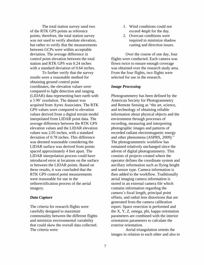
The total station survey used two

of the RTK GPS points as reference

points; therefore, the total station survey

was not used to verify absolute elevation,

but rather to verify that the measurements

between GCPs were within acceptable

deviation. The average difference in

control point elevation between the total

station and RTK GPS was 0.24 inches

with a standard deviation of 0.64 inches.

To further verify that the survey

results were a reasonable method for

obtaining ground control point

coordinates, the elevation values were

compared to light detection and ranging

(LIDAR) data representing bare earth with

a 3.90’ resolution. The dataset was

acquired from Ayres Associates. The RTK

GPS values were compared to elevation

values derived from a digital terrain model

interpolated from LIDAR point data. The

average difference between the RTK GPS

elevation values and the LIDAR elevation

values was 2.05 inches, with a standard

deviation of 0.78 inches. This difference

was deemed reasonable considering the

LIDAR surface was derived from points

spaced approximately 4 feet apart. The

LIDAR interpolation process could have

introduced error at locations on the surface

in between the LIDAR points. Based on

these results, it was concluded that the

RTK GPS control point measurements

were reasonable for use in the

orthorectification process of the aerial

imagery.

Data Capture

The criteria for research flights were

carefully designed to maximize

commonality between the different flights

and minimize environmental variability

that could skew the overall data collected.

The criteria were:

1. Wind conditions could not

exceed 4mph for the day.

2. Overcast conditions were

required to minimize shadow

casting and direction issues.

Over the course of one day, four

flights were conducted. Each camera was

flown twice to ensure enough coverage

was obtained over the research study area.

From the four flights, two flights were

selected for use in the research.

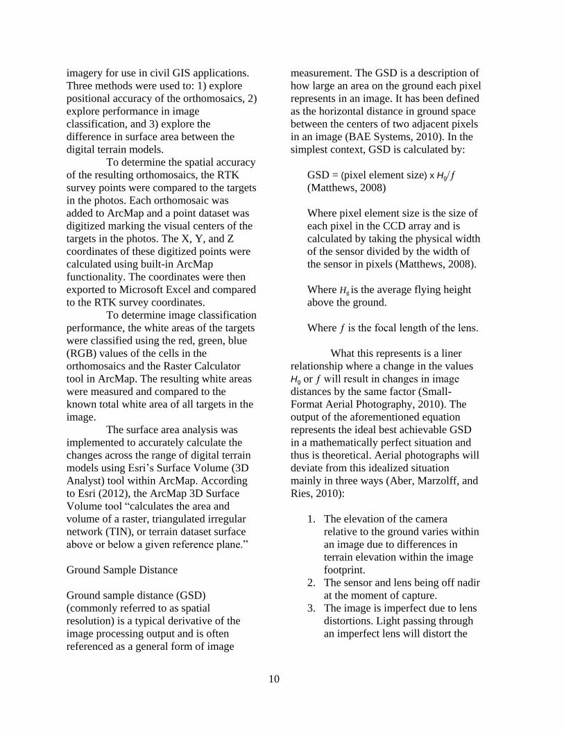
Image Processing

Photogrammetry has been defined by the

American Society for Photogrammetry

and Remote Sensing as “the art, science,

and technology of obtaining reliable

information about physical objects and the

environment through processes of

recording, measuring and interpreting

photographic images and patterns of

recorded radiant electromagnetic energy

and other phenomena (ASPRS, 2009).”

The photogrammetric workflow has

remained relatively unchanged since the

advent of digital photogrammetry. This

consists of projects created where the

operator defines the coordinate system and

ancillary information such as flying height

and sensor type. Camera information is

then added to the workflow. Traditionally

aerial imaging camera information is

stored in an external camera file which

contains information regarding the

camera’s focal length, principal point

offsets, and radial lens distortions that are

generated from the camera calibration

report. Space resection is performed and

the X, Y, Z, omega, phi, kappa orientation

parameters are combined with the interior

orientation parameters to calculate the

exterior orientation.

Aerial triangulation orients the

images in relation to each other and also to

8

the ground coordinate system. This

translates to establish that every pixel

refers to a coordinate. Ground control

points are used both in workflows where

the exterior orientations are known and

unknown. In projects such as this one,

where the exterior orientation is unknown,

ground control points are used to reverse

triangulate for the camera’s interior

orientation using a process known as

exterior camera orientation. The

establishment of an initial approximation

of the orientation parameters (i.e., rough

orientation) is then processed further using

a semi-automatic process in which

additional tie points are identified and

matched throughout corresponding images

to strengthen the matching accuracy. The

final bundle block adjustment is performed

and refined by removing inaccurate points

until the solution is within acceptable error

tolerances.

Digital terrain generation is

performed automatically and the terrain

generation logarithms typically match

terrain points on one or two images.

Ground control points and other data can

often be supplied to help guide the

correlation process. Terrain editing

follows digital terrain generation. This

automated process is to remove and

perform cleanup of extraneous points.

Orthomosaics are typically the final

product derived from the photogrammetric

workflow.

Three distinctly different

photogrammetry applications were chosen

to process the datasets in a side-by-side

comparison: ERDAS LPS, Agisoft

PhotoScan, and Pix4D (described in more

detail below). The objective of using three

photogrammetry applications was to

observe the range of results produced

through data processing.

While the underlying

fundamentals of photogrammetry similarly

span across the applications used in this

study to process the research data, it is

suspected that design of the software, and

for what industry it was made to serve, can

greatly dictate the achievable results from

a standard set of inputs and user defaults.

The defining commonality between the

three chosen applications was the use of

space resection and ground control points

as input. Ground control points were

added into the routines of each application

during the processing of the datasets.

Furthermore, the coordinate system and

projection of the ground control point

inputs were identical, forcing each

application to utilize the same three-

dimensional space when processing the

data.

Orthorectification

Aerial imagery is a representation of

irregular surfaces and texture. Seemingly

flat images are actually distorted due to the

physical curvature of terrain being imaged

and the imaging sensor used. Rectification

is the process of geometrically correcting

the image to be planar so it matches the

corresponding images when in a flat

orientation (ERDAS, 2010).

While not necessary with

featureless flat areas of study,

orthorectification is a more robust form of

rectification that implements digital terrain

models and uses collinerity equations and

ground control points to better compensate

for areas where dramatic changes in

elevation reside (ERDAS, 2010). For the

purpose of this research orthorectification

is used to best represent the data and

analysis.

Software Descriptions

ERDAS LPS is one of the leading

photogrammetry workhorse software

9

programs available today. Owned by

Intergraph Corporation, ERDAS LPS is

tailored for remote-sensing professionals

and large commercial and governmental

agencies. Capable of processing satellite,

LIDAR, aerial imaging, and in some cases

terrestrial datasets, it offers the greatest

range and capability for processing

remotely sensed data. ERDAS LPS offers

the widest range of end-user specified

options of the applications tested, ranging

from terrain elevation model outputs

including accuracy, radiometric quality,

ground sample distance, output projections

and output file format.

Agisoft PhotoScan is a

standalone photogrammetric application

that follows a linear, project-based

workflow. Raw data added to the

workflow requires a camera model be

assigned to each image. This model

consists of the focal length, principal

point, and lens distortion coefficients. This

particular application automatically

applies the Brown model and estimates the

calibration coefficients during processing

(Agisoft, 2012). Should the automatic

calibration fail, calibration parameters are

then entered into Agisoft PhotoScan to

achieve optimal reconstruction results.

Automatic tie point production, based on

detection points of interest and matching,

is first processed. Geometric accuracy

improves with the addition of GCPs being

entered into the project. Next, aerial

triangulation is run, Dense Surface

Reconstruction is processed, and the

resulting digital terrain model (DTM) is

created (Agisoft, 2012). With the digital

terrain model, Agisoft PhotoScan uses a

triangulated irregular network (TIN)

surface to correct for terrain displacement

and exterior orientations for

georeferencing and creation of the

orthoimage (Agisoft, 2012).

Pix4D is both an online service and

stand-alone application specifically

designed for unmanned aerial vehicle

survey imagery datasets. For this research

the automated online service was utilized.

First Pix4D computes the true locations

and parameters of the original images

through Automatic Aerial Triangulation

(AAT) and Bundle Block Adjustment

(BBA). Based on the cloud of 3D points

retrieved during the AAT and the BBA, a

digital surface model is generated by

connecting these points. The number of

3D points is then further increased to reach

up to pixel level point clouds. The

orthomosaic is finally created by

projecting and blending the original

images with the digital surface model.

Processing Outputs

The two flights selected for use in the

research represented one flight with each

image sensor (Canon G10 and Canon

S60). Each application produced one

orthomosaic and one digital terrain model

per set of imagery. The complete catalog

of results consisted of six orthomosaics

and six digital terrain models representing

the complete range of photogrammetry

derived datasets:

1. G10 processed with Agisoft

PhotoScan

2. G10 processed with ERDAS LPS

3. G10 processed with Pix4D

4. S60 processed with Agisoft

PhotoScan

5. S60 processed with ERDAS LPS

6. S60 processed with Pix4D

Functional Measures of Image Quality

Within Esri’s ArcMap software a

systematic approach was devised to assess

the final datasets in order to characterize

the accuracy and overall value of UAV

10

imagery for use in civil GIS applications.

Three methods were used to: 1) explore

positional accuracy of the orthomosaics, 2)

explore performance in image

classification, and 3) explore the

difference in surface area between the

digital terrain models.

To determine the spatial accuracy

of the resulting orthomosaics, the RTK

survey points were compared to the targets

in the photos. Each orthomosaic was

added to ArcMap and a point dataset was

digitized marking the visual centers of the

targets in the photos. The X, Y, and Z

coordinates of these digitized points were

calculated using built-in ArcMap

functionality. The coordinates were then

exported to Microsoft Excel and compared

to the RTK survey coordinates.

To determine image classification

performance, the white areas of the targets

were classified using the red, green, blue

(RGB) values of the cells in the

orthomosaics and the Raster Calculator

tool in ArcMap. The resulting white areas

were measured and compared to the

known total white area of all targets in the

image.

The surface area analysis was

implemented to accurately calculate the

changes across the range of digital terrain

models using Esri’s Surface Volume (3D

Analyst) tool within ArcMap. According

to Esri (2012), the ArcMap 3D Surface

Volume tool “calculates the area and

volume of a raster, triangulated irregular

network (TIN), or terrain dataset surface

above or below a given reference plane.”

Ground Sample Distance

Ground sample distance (GSD)

(commonly referred to as spatial

resolution) is a typical derivative of the

image processing output and is often

referenced as a general form of image

measurement. The GSD is a description of

how large an area on the ground each pixel

represents in an image. It has been defined

as the horizontal distance in ground space

between the centers of two adjacent pixels

in an image (BAE Systems, 2010). In the

simplest context, GSD is calculated by:

GSD = (pixel element size) x Hg/ƒ

(Matthews, 2008)

Where pixel element size is the size of

each pixel in the CCD array and is

calculated by taking the physical width

of the sensor divided by the width of

the sensor in pixels (Matthews, 2008).

Where Hg is the average flying height

above the ground.

Where ƒ is the focal length of the lens.

What this represents is a liner

relationship where a change in the values

Hg or ƒ will result in changes in image

distances by the same factor (Small-

Format Aerial Photography, 2010). The

output of the aforementioned equation

represents the ideal best achievable GSD

in a mathematically perfect situation and

thus is theoretical. Aerial photographs will

deviate from this idealized situation

mainly in three ways (Aber, Marzolff, and

Ries, 2010):

1. The elevation of the camera

relative to the ground varies within

an image due to differences in

terrain elevation within the image

footprint.

2. The sensor and lens being off nadir

at the moment of capture.

3. The image is imperfect due to lens

distortions. Light passing through

an imperfect lens will distort the

11

true representation of the physical

area (Aber et al., 2010).

In order to assess the variability in how

accurately the applications interpret GSD

compared to the theoretical GSD, an

analysis was completed determining GSD

at three points in the project workflow:

1. Using the above equation with the

average elevation input based upon

geo-tagged imagery information.

2. Using the above equation with

elevation based upon the

photogrammetry application’s

external orientation estimation.

3. Using the photogrammetry

application’s bundle adjusted

output reported GSD (the cell size

of the resulting orthomosaics).

Results

Camera Calibration

The results of the camera calibration are

summarized here to compare results from

the three camera calibration objects and

the results from calibrations before and

after flight. A detailed examination of the

calibration results is beyond the scope of

the research but is summarized to illustrate

the discrete variations present between

calibrations. The three parameters

considered of highest importance were

focal length, principle point, and radial

distortion for two reasons. First, these are

the characteristics typically required by

photogrammetry software, and second,

these parameters are subject to change by

external and environmental forces such as

shock, air pressure, temperature and

humidity. This can lead to inconsistency in

the photogrammetric process where

interior camera orientation parameters are

required.

Focal length of both cameras did

show changes between calibrations

(Figure 7). The Canon G10 was initially

calibrated with a focal length of 6.3891

mm using the USGS cage. Its focal length

was shown to vary on average by 9.367

µm in subsequent calibrations. The Canon

S60 was initially calibrated with a focal

length of 6.0271 mm using the USGS

cage. Its focal length was shown to vary

on average by 2.967 µm in subsequent

calibrations, 6.4 µm less compared to the

G10.

Figure 7. Focal length (mm) results from the

camera calibration objects for the Canon G10

(blue) and Canon S60 (green) pre- and post-flight.

Radial distortion correction is the

measure of how much each image would

need to be corrected to remove the

distortion calculated by the calibration

procedure. It is therefore feasible to

correlate the variances in correction values

to movement of the internal lens elements.

The radial distortion observed did show

changes between calibrations (Figure 8).

For the Canon G10 the greatest change

from the USGS cage control calibration

was observed in the USGS box calibration

(20 µm at 4.5 mm radius). For the Canon

S60 the greatest change from the USGS

cage control calibration was observed in

6.3

891

6.3

835

6.4

035

6.3

972

6.0

271

6.0

216

6.0

256

6.0

252

5.4

5.6

5.8

6

6.2

6.4

6.6

6.8

7

Cag

e

US

GS

Bo

x

Fie

ld B

ox

Fie

ld B

ox

Cag

e

US

GS

Bo

x

Fie

ld B

ox

Fie

ld B

ox

Fo

cal

Len

gth

(m

m)

Calibration Device

Focal Length:G10 and S60, Pre and Post Flight

G10 S60

Pre-Flight Post Pre-Flight Post

12

the USGS box calibration (15 µm at 4.5

mm radius).

Figure 8. Radial Distortion ( m) analysis output

from the camera calibration objects (solid lines)

and difference from the USGS cage ( m; dashed

lines) for the Canon S60 (top) and Canon G10

(bottom).

The principal point, according to

Eos Systems, Inc. (2010), is “the location

in a camera where the optical axis of the

lens intersects the imaging plane. It is the

reference point in the image to which all

marks and lens distortion parameters are

related.”

In practice, the principal point

will deviate off axis of center and is

calculated as a correction in the camera

calibration report. For each of the cameras

it is shown that that the principal point was

not stable and did shift in each calibration

performed (Figure 9).

Figure 9. Principal Point calibration correction

(mm) analysis. Change between calibrations is

represented in xp, yp.

Functional Performance Measures

Ground Sample Distance Analysis

Each photogrammetry software reported a

calculated GSD of the resulting

-20

-15

-10

-5

0

5

0

50

100

150

200

250

0 1 2 3 4 5

Diffe

ren

ce fro

m U

SG

S C

ag

e (d

ash

ed

lines)

Dis

tort

ion

(m

icro

ns (µ

m))

Radius (mm)

Radial Distortion Correction: S60

Cage (Pre) USGS Box (Pre)

Field Box (Pre) Field Box (Post)

-20

-15

-10

-5

0

5

0

50

100

150

200

250

0 1 2 3 4 5

Radius (mm)

Radial Distortion Correction: G10

Cage (Pre) USGS Box (Pre)

Field Box (Pre) Field Box (Post)

Dis

tort

ion

(m

icro

ns (µ

m))

Diffe

ren

ce fro

m U

SG

S C

ag

e (d

ash

ed

lines)

-0.06

-0.04

-0.02

0

0.02

0.04

0.06

-0.1 -0.08 -0.06 -0.04 -0.02 0 0.02

Calibration Determined Principal Point

G10 Cage (Pre) G10 Field Box (Pre)

G10 USGS Box (Pre) G10 Field Box (Post)

S60 Cage (Pre) S60 Field Box (Pre)

S60 USGS Box (Pre) S60 Field Box (Post)

13

orthoimagery (Table 1). On average

ERDAS produced the largest GSD at 2.33

cm per pixel, followed by Pix4D with 2.30

cm per pixel and Agisoft PhotoScan 1.92

cm per pixel using both camera datasets.

Table 1. Final ground sample distance (GSD) for

imagery obtained by the Canon G10 and Canon

S60 and processed with one of three

photogrammetry software packages.

Software Camera GSD (cm/pixel)

ERDAS LPS G10 1.82

S60 2.3

Pix4D G10 1.10

S60 3.50

Agisoft PhotoScan

G10 1.21

S60 2.63

The analysis comparing the two

cameras shows the Canon G10 averaged a

GSD of 1.3 cm per pixel. The Canon S60

showed an average GSD of 2.99 cm per

pixel, a 130% increase over the Canon

G10.

These post-processed GSD

results were compared to the pre-

processed theoretical GSD predictions

calculated using the equation described in

the methods (Figure 10). The theoretical

GSD was calculated once using the

average camera elevation based on image

geotag information and again based on the

camera’s external orientation determined

by the software.

The results show the resulting

GSD for both PhotoScan datasets were

better than expected. This is likely to due

GPS’s inherent lack of vertical precision

causing error in initial elevation estimates

which were later corrected by the

software. The Pix4D Canon S60 GSD

calculated using the software’s estimated

external camera orientation show the most

difference from predicted values. This

appears to be due to an anomaly in how

the software interpreted the geotagged

image elevation. However, the final

resulting GSD values were within

expected tolerances.

Figure 10. Ground sample distance (GSD) for

imagery obtained by the Canon G10 and Canon

S60: based on photo geotag elevation (blue), based

on software determined external camera orientation

information (red), and final cell size of

orthoimagery (green).

Ground Control Point Accuracy

Comparison

Ground control point accuracy was

examined by comparing the RTK GPS

control points locations against visual

target locations for each orthomosaic. The

distance was measured from the center of

each aerial target to the corresponding

ground control point. The differences in X

and Y directions from the target center

were documented (Figure 11).

0.0

0.5

1.0

1.5

2.0

2.5

3.0

3.5

4.0

G10 E

rdas

G10 P

ix4D

G10 P

hoto

Scan

S60 E

rdas

S60 P

ix4D

S60 P

hoto

Scan

GS

D (cm

)

Ground Sample Distance: Predicted and Result

Average Geotag Elevation

Software External Camera Orientation

Resulting Cell Size

14

Canon G10 imagery processed

with Agisoft PhotoScan resulted in 2.14

cm average error and Canon S60 imagery

processed with Agisoft PhotoScan had an

average 2.10 cm error. The averaged error

was 2.12 cm. Pix4D combined average

error was 9.312 cm and ERDAS’s average

was shown to be 10.25 cm in error (Figure

12).

Figure 11. Scale GCP error representation of

ERDAS processed G10 imagery in relation to a

sample aerial target.

DTM Analysis

The examination of the digital terrain

models resulted in an observed trend

between smaller GSD and increased 3D

surface area. Where the Agisoft PhotoScan

Canon G10 dataset proved to have the

highest 3D surface area of 10,477.52 ft2,

the ERDAS Canon S60 was shown to have

the lowest 3D surface area of 9896.62 ft2.

This represents a 5.87% decrease in total

surface area (Figure 13).

Pixel Classification

The image pixel classification analysis

was implemented to calculate from within

ArcMap the difference between the known

total white area of the aerial targets versus

Figure 12. Ground control point (GCP) error index.

The direct comparison between camera and

application.

Figure 13. Difference in 3D surface area per

application represented in square feet and

percentage change from PhotoScan G10.

40 cm

- 40 cm

40 cm- 40 cm

y

x

PH

OT

OS

CA

NP

IX4D

ER

DA

S

CANON S60CANON G10

-40

0

40

-40 0 40

-40

0

40

-40 0 40

-40

0

40

-40 0 40

-40

0

40

-40 0 40

-40

0

40

-40 0 40

-40

0

40

-40 0 40

Centimeters

-6

-4

-2

0

2

4

6

8

10

12

149,600

9,700

9,800

9,900

10,000

10,100

10,200

10,300

10,400

10,500

10,600

% C

han

ge f

rom

Ph

oto

Scan

G10

3D

Are

a (

Sq

uare

Feet)

3D Surface Area of DEM

3D Area (Square Feet)

15

the orthoimage classified white area

(Figure 14). Pix4D processed Canon S60

imagery represented a 9.04% increased

area. The greatest difference was observed

in Canon G10 Pix4D at a 13.477%

increase. The results were inconclusive

and will be discussed further below.

Figure 14. Image classification analysis. Known

area of the white area of the aerial targets (black

bars) compared to the resulting area found by

image classification (light grey bars).

Discussion

Sources of Error

The probable sources of error in this

research are mainly:

1) The altitude variability above the

ground and overlap of images.

Mosaicing and processing images

from dramatically different

altitudes and overlaps is not ideal.

Images that are consistently of the

same overlap and elevation above

ground would reduce error.

2) Variability in the environmental

conditions between the flights.

Atmospheric conditions such as

turbulence, wind speed, humidity

and available ambient light are

notable variable factors between

the data collection flights.

3) Lens and sensor variability

between calibrations. Mechanical

variability in the non-metric

variable zoom camera lenses used

in this research may introduce

error. Variability may be caused by

external shock or vibration upon

the camera. Variation may be

caused by relative temperature or

humidity acting on the camera’s

materials. Variability may be a

result of the combination of the

aforementioned factors.

4) Human error. User interpretation of

the aerial target image centers and

the manual selection of ground

control point entry for each

software package could vary. Error

could also exist during software

project setup and in procedural

fine-tuning.

5) Aircraft performance from flight to

flight. Physical changes to the

aircraft, center of gravity,

equipment configuration or

position could affect a change in

how the aircraft would fly from

one flight to the next.

6) Minimal sampling of datasets in

both the camera calibrations and

flights. Due to the window of

opportunity to conduct the imaging

research flights, only a limited

number of flights were completed.

To reduce sampling error more

flights should be flown and more

samples should be included.

2812.5

2812.5

2587.5

2812.5

2812.5

2812.5

3,2

80.6

7

3,0

95.2

2

2,9

36.2

3

3,1

36.9

3

3,1

61.3

0

3,0

66.8

6

0

500

1000

1500

2000

2500

3000

3500

Sq

uare

In

ch

es

Camera / Software

Image Classification Area: Known vs. Observed

Predicted White Square Inches

White Square Inches

16

Camera Calibration Stability

The camera calibrations have illustrated

that there is variability in the lenses and

that the calibrations are not consistent

when compared across the range of

cameras and calibration objects used in

this research. When the pre and post field

box calibrations for the Canon G10 and

Canon S60 were compared, variability was

still observed between calibrations, with

the Canon G10 having a 5.2 µm difference

in radial distortion at 4.5 mm and Canon

S60 having a 3.2 µm difference in radial

distortion at 4.5 mm. However, it appears

that the variability observed in the

calibrations may be compensated for in the

post-processing of datasets.

Camera Performance

The Canon G10 camera was expected to

produce higher resolution imagery over

the Canon S60 strictly based on the Canon

G10 higher theoretical sensor and lens

capabilities. This correlation was observed

in the GSD analysis where Canon G10

cm/pixel results were consistently of a

higher resolution than the Canon S60. The

GCP accuracy comparison analysis

indicates that the Canon G10 and Canon

S60 were virtually identical. Variances in

the values were too small to draw a

definite conclusion as to which camera

preformed better in this test. This could be

affected due to where the image centers

were interpreted.

The DTM analysis sought to

compare the three dimensional area of the

DTMs. The goal was to observe if a higher

resolution DTM would affect the total

three dimensional surface area and what, if

any, relationship existed between the

DTMs and GSDs. The PhotoScan Canon

G10 dataset yielded the largest 3D surface

area at 10477.52 ft2 followed by the Pix4D

Canon G10 dataset at 10301.11 ft2. The

third largest surface area dataset was the

Pix4D Canon S60 dataset with a 3D area

of 10233.88 ft2, narrowly exceeding the

ERDAS Canon G10 with a 3D area of

10229.55 ft2 by just 4.33 ft

2. The results

are somewhat surprising being that the

Pix4D Canon S60 dataset had more

surface area than the ERDAS Canon G10

even though the Pix4D Canon S60 dataset

had a larger GSD than the ERDAS Canon

G10.

Software Performance

ERDAS LPS, a traditional production

level photogrammetry application for

commercial and government wide-area

imaging is vastly more robust and

complex than the other two applications in

the study. However, its routines and

logarithms are generally specific in terms

of what the application expects as input

data. ERDAS LPS expects data to be

generally from the same altitude and of

near nadir at the time of capture. ERDAS

LPS was designed to process imagery

from manned piloted aerial aircraft and

satellite imaging where altitude above the

ground can be tightly controlled and

reported. Furthermore, the pitch, roll, and

yaw angles of the aircraft are more easily

controlled by employing sophisticated

gimbal systems that allow the imaging

sensor to maintain near nadir position

during data capture. Initial findings of this

research appear to show that consistency

in image overlap and altitude has a larger

effect on the overall accuracy when the

application workflow is expecting this

type of imagery. The Canon G10 ERDAS

imagery was taken from various elevations

and off-nadir orientations throughout the

flight (Figure 15), whereas the Canon S60

imagery was taken as a single series of

images along one flight line (Figure 16).

17

The GSD results for the Canon

G10 imagery processed with ERDAS LPS

was natively better than the Canon S60

due to the sensor size; however, it was

worse than the geotag elevations would

have predicted. This difference is likely

due to the software not anticipating images

from dramatically different elevations and

orientations off nadir.

Figure 15. Screen capture of the ERDAS LPS

interface illustrating the Canon G10 image

footprints in the Block file. Note the variations in

footprint size and orientation.

Figure 16. Screen capture of the ERDAS LPS

interface illustrating the Canon S60 image

footprints in the Block file. Note the consistency in

footprint size and orientation.

Improvements in final GSD

relative to predicted GSD were seen with

both the Pix4D and PhotoScan

applications, suggesting these programs by

design are likely less sensitive to variation

in image elevation than ERDAS LPS.

Whereas the applications ERDAS

LPS and Agisoft PhotoScan accept interior

orientation information input to obtain

exterior camera orientation, Pix4D does

not require interior orientation information

as an input, possibly affecting overall

quality.

Image Performance

There was variability found in the analysis

of the datasets processed in ArcMap. The

image classification analysis sought to

calculate within ArcMap the difference

between the known total white area of the

aerial targets vs. the observed

classification area within the derived

datasets. The results obtained from the

image classification were not expected. A

trend was expected between GSD and

classification accuracy where more

accurate classification results would be

expected with smaller GSD. This trend

was not observed possibly due to: 1) the

phenomenon called image bloom where

brighter areas of an image grow relative to

their actual size, and 2) inaccurate

classification parameters used in analysis.

More work could be done in the future to

refine the parameters or test alternative

image classification scenarios.

Variability and consistency are

the largest hurdles that need to be

addressed when assessing the capabilities

of UAV survey systems against

commercial aerial imagery products.

Considerations of how environmental and

procedural variability can affect the

datasets need to be addressed and if that

variability is within acceptable tolerances

for the project at hand. Additional

sampling and testing needs to be

conducted in order to develop a truly

accurate measure of the variability

observed in the research.

Future Research

Future research would seek to extend upon

the initial findings of this research. First,

to conclude that any specific unmanned

18

aerial survey vehicle can produce a dataset

of certain quality, it is the author’s

assertion that claims of capability should

be based upon dozens, if not multiple

dozens of nearly identical data collection

flights. Second, moving beyond multiple

sensors and multiple image processing

applications, one camera sensor and one

image processing application should be

chosen for the future research to provide

consistency over the range of future

flights. If there is any doubt regarding a

particular application or sensor, the

examination of other cameras and

application combinations could be

explored utilizing the above methodology

of testing one sensor against one

application.

Conclusion

The research has illustrated a process for

comparing unmanned aerial survey

datasets from two cameras and processed

through three photogrammetry software

applications. The analysis for the research

was conducted solely from within the Esri

GIS environment and was intended to

identify and isolate the relationships

between the cameras and software where

possible. The research suggests the

process and methodology is capable of

producing high-resolution spatially

accurate data that is comparable if not

better than current commercial

deliverables for small areas of study. With

typical current commercial imagery

provided at 15.24 cm GSD, this research

was able to achieve 1.92 cm GSD.

Reliability and consistency of the

cameras was analyzed from comparisons

in the calibration. Reliability and

consistency of the cameras was observed

to be acceptable. The photogrammetry

applications used in the research appear to

expect some variation and are able to

compensate for that variable input and still

produce reasonable results. Spatial

accuracy was tested by comparing where

the aerial targets centers resided in the

images to the actual GCP coordinates. The

overall spatial accuracy achieved in the

research should be considered accurate

enough to service small areas of research

where aerial remote sensing is needed but

would be otherwise be too cost-prohibitive

and time-sensitive to fulfill with traditional

commercial aerial datasets. Project

findings support the value of continued

research into unmanned aerial survey

vehicles in conjunction with non-metric

cameras to produce viable geospatially

accurate datasets.

Acknowledgements

Special thanks to the following individuals

and organizations that have contributed to

this research:

Larry Hanson

Al Slavick

Joerg Feldbinder of Paragon

Associates

Don Moe of the USGS

John Ebert of Saint Mary’s

University

Dr. McConville of Saint Mary’s

University

Greta Bernatz of Saint Mary’s

University

Jerome Johnson of Winona State

University Composite Materials

Engineering program

Don Ritzenthaler

Al Poser

Patricia Poser

References

Aber, J. S., Marzolff, I., and Ries, J. B.

2010. Small-Format Aerial Photography:

19

Principles, Techniques and Geoscience

Applications. Elsevier. Oxford, UK.

Abramson, L. 2012. Drones Drifting Into

Markets Outside War Zones. National

Public Radio. Retrieved September 19,

2012 from http://www.npr.org/

2012/08/13/158715809/drones-drifting-

into-markets-outside-war-zones.

Agisoft. 2012. Agisoft PhotoScan –

Capabilities. Retrieved September 19,

2012 from http://www.agisoft.ru/wiki/

PhotoScan/Capabilities.

American Society of Photogrammetry and

Remote Sensing (ASPRS). 2009.

Guidelines for Procurement of

Professional Aerial Imagery,

Photogrammetry, Lidar and Related

Remote Sensor-based Geospatial

Mapping Services. Retrieved September

3, 2012 from http://www.asprs.org/

a/society/committees/standards/

Procurement_Guidelines_w_accompanyi

ng_material.pdf.

BAE Systems. 2010. Glossary of Terms.

Retrieved from http://www.socetgxp.

com/docs/support/ socet-gxp_glossary-

of-terms.pdf.

Canon. 2012a. About PowerShot G10.

Retrieved September 2, 2012 from

http://www.usa.canon.com/cusa/support/

consumer/digital_cameras/powershot_g_

series/powershot_g10#Specifications.

Canon. 2012b. About PowerShot S60.

Retrieved September 2, 2012 from

http://www.usa.canon.com/cusa/support/

consumer/digital_cameras/powershot_s_

series/powershot_s60#Specifications.

Eos Systems, Inc. 2010 Glossary.

Retrieved November 29, 2012 from

http://www.photomodeler.com/support/g

lossary.htm.

ERDAS. 2010. ERDAS Field Guide.

ERDAS, Inc. Norcross, GA.

Matthews, N. A. 2008. Aerial and Close-

Range Photogrammetric Technology:

Providing Resource Documentation,

Interpretation, and Preservation.

Technical Note 428. U.S. Department of

the Interior, Bureau of Land

Management, National Operations

Center, Denver, Colorado. 42 pp.

Retrieved September 25, 2012 from

http://www.blm.gov/nstc/library/pdf/TN

428.pdf.

Professional Aerial Photographers

Association. 2012. History of Aerial

Photography. Retrieved September 3,

2012 from http://www.papainternational

.org/ history.asp.

Stahlke, E. 2011. Aerial Perspective:

Close-range Aerial Photogrammetry

Comes of Age. Professional Surveyor

Magazine. Retrieved September 2, 2012

from http://www.profsurv.com/

magazine/article.aspx?i=70968.

20

Appendix A. Project Imagery of Study Area.

The ArcMap layout above illustrates the research imagery’s orthomosaic spatial orientation and scale in relation

to Microsoft’s Bing Map base layer.