Proceedings of IMECE 2004

2004 ASME International Mechanical Engineering Congress

Anaheim, California, USA, November 13-19, 2004

IMECE 2004-61323

COMPACT MODELS FOR TRANSIENT CONDUCTION OR VISCOUS TRANSPORT

IN NON-CIRCULAR GEOMETRIES WITH A UNIFORM SOURCE

Y.S. Muzychka∗

Faculty of Engineering and Applied Science

Memorial University of Newfoundland

St. John’s, NL, Canada, A1B 3X5

M.M. Yovanovich†

Department of Mechanical Engineering

University of Waterloo

Waterloo, ON, Canada, N2L 3G1

ABSTRACT

Transient heat conduction in solid prismatic bars ofconstant cross-sectional area having uniform heat genera-tion and unsteady momentum transport in infinitely longducts of arbitrary but constant cross-sectional area are ex-amined. In both cases the solutions are mathematicallymodeled using a transient Poisson equation. By means ofscaling analysis a general asymptotic model is developed foran arbitrary non-circular cross-section. Further, by meansof a novel characteristic length scale, the solutions for anumber of fundamental shapes are shown to be weak func-tions of geometry. The proposed models can be used topredict the dimensionless mean flux at the wall and thearea averaged temperature or velocity for the tube, annu-lus, channel and rectangle for which exact series solutionsexist. Due to the asymptotic nature of the proposed mod-els, it is shown that they are also applicable to other shapesat short and long times for which no solutions or data exist.The root mean square (RMS) error based on comparisonswith exact results is between 2.2-7.6 percent for all dataconsidered.

KEYWORDS: Unsteady Viscous Flow, Unsteady HeatConduction, Modelling, Asymptotic Analysis, Scale Anal-ysis, Poisson Equation

NOMENCLATURE

A = area, m2

A0, A∞ = closure constantsB0, B∞a, b = major and minor axes of rectangle, m

= outer and inner radii, mDh = hydraulic diameter, ≡ 4A/PfReL = friction factor Reynolds number group

≡ 2PoLG = source parameterJ0(·) = Bessel function of first kind order zero

∗Assistant Professor†Distinguished Professor Emeritus, Fellow ASME

k = thermal conductivity, W/mKL = duct or channel length, mL = arbitrary length scale, mm,n = series indicesn, p = asymptotic correlation parametersn = directed normal, mN = number of sides of a polygonp = pressure, PaP = perimeter, mPoL = Poiseuille number, ≡ τL/µwqs = surface heat flux, W/m2

r = radial coordinate, mr∗ = radii ratio, b/aReL = Reynolds number, ≡ wL/νs = arc length, mS = volumetric heat generation, W/m3

t = time, st? = dimensionless time,≡ βt/L2

w = velocity, m/sw = average velocity, m/sx, y, z = cartesian coordinates, mY0(·) = Bessel function of second kind order zero

Greek Symbols

α = thermal diffusion coefficient, m2/sβ = general diffusion coefficient, m2/sδ = boundary layer thickness, mδn = eigenvalueε = aspect ratio, b/aφ = independent variable, θ or w

φ? = dimensionless transport quantity, ≡ φ/GL2

φn = gradient of φ, ≡ ∂φ/∂nγ = transport coefficient, k or µη = similarity variableλmn = eigenvalueµ = dynamic viscosity, Ns/m2

ν = kinematic viscosity, m2/sθ = temperature excess, K

1

ρ = density, kg/m3

% = dimensionless radial position, r/aψ = flux, W/m2 or N/m2

φ? = dimensionless flux, ≡ φnP/AGτw = wall shear stress, Pa

Subscripts

s = surfacew = wall∞ = steady state valueL = based upon the arbitrary length L

Superscripts

(·) = mean value(·)? = dimensionless value

INTRODUCTION

This paper is concerned with the analysis of unsteadytransport of momentum due to a suddenly imposed con-stant pressure gradient or unsteady heat conduction due toa uniformily distributed heat source in circular and non-circular geometries.

The viscous transport problem which is most oftenfound in advanced level fluids texts [1-5], is concerned withstart up flow in circular and non-circular tubes and chan-nels. The solution for a tube was originally found by Szy-manski [6] in 1932. In addition to the circular tube, solu-tions for the parallel plate channel [7,8], circular annulus [9],and rectangle [10], are also available in the fluids literature.The solution for the channel is discussed in Rouse [7] andArpaci and Larsen [8] with no reference to its origins. Thesolution may be traced back to Lamb [11] as early as 1927.Lamb [11] used a Fourier series method to obtain the so-

lution, but later Bromwich [12] obtained a similar solutionusing Laplace transforms [12,13]. The solution for the cir-cular annulus was obtained by Muller [9] in 1936. While thesolution for a rectangular channel may be found in Erdo-gan [10], but elements of its solution are discussed in earliermathematical works [14-17]. The solution for the rectangleas presented by Erdogan [10] is somewhat complex and hasbeen re-solved using Fourier transforms [18-20] as part ofthe present work to provide a more compact form.

The viscous transport problem also has an analogousconterpart in conduction heat transfer. The temperaturefield which results from a uniformily distributed heat sourcewhich is suddenly turned on is governed by a similar dif-ferential equation and boundary and initial conditions [21].Carslaw and Jaeger [21] discuss both the plane wall andcircular cylinder solutions for transient conduction with aconstant uniform heat source. A solution for the annularcylinder is not presented, but cited by Thews [22]. No ref-erence to any solution for a rectangular domain is made.

The paper reviews the aforementioned analytical solu-tions and considers the characteristics of these solutions.Simple models are proposed for calculating these charac-teristics which make computations more amenable. Twoadvantages of these compact models will become appar-ent. First, the available solutions are in the form of infiniteseries. In the case of the rectangle a double inifinite se-ries is required. Further, the solutions for the cylinder andannulus involve Bessel functions and the eigenvalues mustbe numerically computed from expressions involving thesefunctions. Second, the analysis will show that the resultsare applicable to other useful geometries for which no so-lutions exist, i.e. the elliptic duct, triangular duct, andpolygonal ducts (refer to Fig. 1).

y

x

Rectangle

a ≥ b

x

y

0 0

Ellipse

a ≥ b

x y = 1

a b

+

Semi-Circle

ba

ba

2 2

= 1+ a b

x yn n

n <0 < ∞

0.000 0.200 0.400 0.600 0.8000.000

0.200

0.400

0.600

0.800

1.000

0.000 0.200 0.400 0.600 0.8000.000

0.200

0.400

0.600

0.800

1.000

Hyper-Ellipse

a ≥ b

x

y

ba

0

Square

N = 3

Triangle Pentagon

N = 4 N = 6 N → ∞Hexagon Circle

N = 5

Fig. 1 - Typical Non-Circular Cross-Sections.

2

With respect to the problem of interest, two funda-mental quantities are useful to the engineer for modelingthe transient response of a system. One is the dimension-less area averaged velocity or temperature (potential), andthe other is the dimensionless perimeter averaged wall shearor heat flux (gradient of potential). Since the solutions tothese problems involve infinite single and double series, it isdesirable to have compact models for computing the desiredparameters. Simple models will be proposed for both thedimensionless average potential and dimensionless averagegradient of the potential.

In general, the results presented in this work are ap-plicable to any unsteady Poisson equation with constantuniformily distributed source, constant physical properties,and homogeneous Dirichlet boundary conditions. Next themathematical statement for each problem is discussed andpresented in a general form.

PROBLEM STATEMENT

The problem of interest is characterized by the follow-ing general Poisson equation:

1

β

∂φ

∂t= G + ∇2φ (1)

which is subject to the boundedness condition along theaxis of the geometry, φ 6= ∞, homogeneous Dirichlet con-ditions at the boundary, φ = 0, and the initial conditionφ = 0, when t = 0. The system is shown in Fig. 2. It con-sists of an infinitely long duct or cylinder of arbitary butconstant cross-sectional area, A, bounded by perimeter, P .

It is of interest to obtain the area mean potential, ob-tained by integrating the solution for φ over the cross-sectional area:

φ(t) =1

A

∫ ∫

A

φdA (2)

Also, of interest is the perimeter averaged or mean gra-

dient at the surface,∂φ

∂n≡ φn:

ψ(t) =1

P

∮

γ∂φ

∂nds = γφn (3)

which is related to the momentum flux or heat flux throughthe appropriate thermophysical property for γ using New-ton’s law or Fourier’s law. The two fundamental transportproblems are summarized below in Table 1

Table 1Summary of Variables

Problem φ β G γ ψ

Momentum w ν1

µ

∆p

Lµ τw = µ

∂w

∂n

Conduction θ αSk

k qs = k∂θ

∂n

Fig. 2 - System Under Consideration.

Unsteady Viscous Transport The momentum trans-port or impulsively started flow problem is often classifiedin some texts as Rayleigh flow, Telionis [4]. In other textsit is referred to as startup flow or the commencement ofPoiseuille flow. In this problem, the source is defined as

G =1

µ

∆p

L. The dimensionless mean velocity is:

w? =w

L21

µ

∆p

L

=φ

GL2= φ? (4)

While the dimensionless momentum flux (or shearstress) at the surface is defined with respect to the steadystate value:

τ? =τw

τ∞(5)

where

τ∞ =A

P

∆p

L(6)

is obtained from the steady state force balance.This leads to the following result for the dimensionless

momentum flux or wall shear:

τ? =τw

A

P

∆p

L

=µφn

A

P

∆p

L

=φn

A

PG

= ψ? (7)

Unsteady Heat Conduction In the case of unsteadyheat conduction with a source, similar dimensionless groupsmay be defined. In this problem, the source is defined asG = S/k. The dimensionless mean temperature in thecross-section is:

θ? =θ

L2Sk

=φ

GL2= φ? (8)

While the dimensionless heat flux at the surface is de-fined with respect to the steady state value:

q? =qs

q∞(9)

where

q∞ =A

PS (10)

is obtained from the steady state heat balance.

3

This leads to the following result for the dimensionlessheat flux:

q? =qs

A

PS

=kφn

A

PS

=φn

A

PG

= ψ? (11)

In later sections, we will examine exact results and ap-proximate results for the two dimensionless quanties, φ?

and ψ?. In the next section, we use scale analysis to ob-tain the order of magnitude behaviour for both quantitiesin terms of asymptotic limits.

SCALE ANALYSIS

In this section, we will examine what information themethod of scale analysis [23] may provide. Recall, thetransport equation:

1

β

∂φ

∂t︸ ︷︷ ︸

Storage

= G︸︷︷︸

Generation

+ ∇2φ︸︷︷︸

Diffusion

(12)

This equation represents a balance of three quantities:storage, generation, and diffusion. There are three distinctflow regions in this problem that may be considered. Fullydeveloped flow exists after a very long time, and at shorttimes, there exists a potential core and a very thin bound-ary layer region. Each of these regions may be analyzed us-ing scale analysis. The following scales will be used: φ ∼ φ,t ∼ t, and ∇2 ∼ 1/L2 for long time and ∇2 ∼ 1/δ2 for shorttime. Here, L is as yet undetermined characteristic lengthscale related to the geometry and δ is the boundary layerthickness or penetration scale associated with early times.

First for long times t → ∞, or fully developed flow, thebalance between generation and diffusion leads to ∇2 ∼1/L2. This gives

φ

L2∼ G (13)

or

φ ∼ GL2 (14)

or

φ?∞ =

φ

GL2∼ 1 as t → ∞ (15)

Next, for short times t → 0, the balance is betweenstorage and generation, or considering the potential core,this leads to

1

β

φ

t∼ G (16)

or

φ ∼ Gβt (17)

or

φ?0∼ βt

L2∼ t? as t → 0 (18)

Next, in the boundary layer region, the balance be-tween storage and diffusion leads to ∇2 ∼ 1/δ2. This gives

1

β

φ

t∼ φ

δ2(19)

orδ ∼

√

βt (20)

which is the intrinsic penetration depth.The flow becomes fully developed when δ ∼ L, such

that

βt ∼ L2 (21)

or

t? ∼ βt

L2∼ 1 (22)

Finally, we wish to develop expressions for the meanflux at the surface defined as:

ψ = γ∂φ

∂n(23)

We must consider the two limiting cases of short timeand long time. For long time, t → ∞, the flux becomes:

ψ ∼ γφ

L (24)

We may also relate the flux to the source G for fullydeveloped flows, where

ψ∞ =A

PGγ (25)

Thus, if we define ψ? = ψ/ψ∞, we obtain

ψ?∞ =

φ(

A

PGL

) ∼ 1 as t → ∞ (26)

Finally, for short times, t → 0, the flux becomes

ψ ∼ γφ

δ(27)

Also, from the transport equation we see that

φ

δ2∼ G (28)

or, after combining Eqs. (27) and (28):

ψ ∼ γGδ (29)

Finally defining ψ? as before, we obtain

ψ?0∼ δ

A/P∼

√t?L

A/Pas t → 0 (30)

It is clear from scaling analysis, that two distinct char-acteristics are present. These are the dimensionless meanpotential, φ? and dimensionless mean surface flux, ψ?.Each has the following asymptotic behaviour:

φ? =

A0t? t? → 0

A∞ t? → ∞(31)

and

ψ? =

B0

√t? t? → 0

B∞ t? → ∞(32)

4

Later, an approximate model is obtained by superpos-ing these asymptotes. But first we examine the exact so-lutions for each of these regions in order to determine theclosure constants A0, A∞, B0, and B∞.

ASYMPTOTIC BEHAVIOUR

The exact asymptotic behaviour for small and largetimes may now be examined for each dimensionless quan-tity of interest.

Long Time - t → ∞ For long time, t → ∞, the flowis characterized by a balance between generation and diffu-sion. This problem has been analyzed extensively for mo-mentum transport and solutions to some forty configura-tions may be found in Shah and London [24]. The resultsare usually presented in the form of the dimensionless groupfRe, the Fanning friction factor Reynolds number productdefined as:

fReL2

=τ∞Lµw

=ψ∞Lγφ

= PoL (33)

where Po is referred to in the fluids literature as thePoiseuille number [4].

We can further introduce the source term through thefully developed flow balance Eq. (25) and obtain:

PoL =ψ∞Lγφ

=

A

PGL

φ(34)

Rearranging, for φ and using the definition of the di-mensionless mean potential, Eq. (4) or Eq. (8), we obtain

φ? =A/P

PoLL(35)

which gives

A∞ =A/P

PoLL(36)

Finally, by virtue of the definition of the dimension-less flux, Eq. (5) or Eq. (9) and the value for ψ∞, thedimensionless asymptotic limit for ψ? is:

ψ? = 1 (37)

which gives

B∞ = 1 (38)

Short Time - t → 0 For short times, t → 0, the trans-port is characterized by a balance between generation andstorage. The equation of transport which may be solved inthe potential core when δ is small is:

1

β

∂φ

∂t= G (39)

This may be integrated and solved with the initial con-dition φ(0) = 0 to give:

φ(t) = βtG ≈ φ(t) (40)

When non-dimensionalized, the solution for short timein the potential core is:

φ? =βt

L2= t? (41)

which gives

A0 = 1 (42)

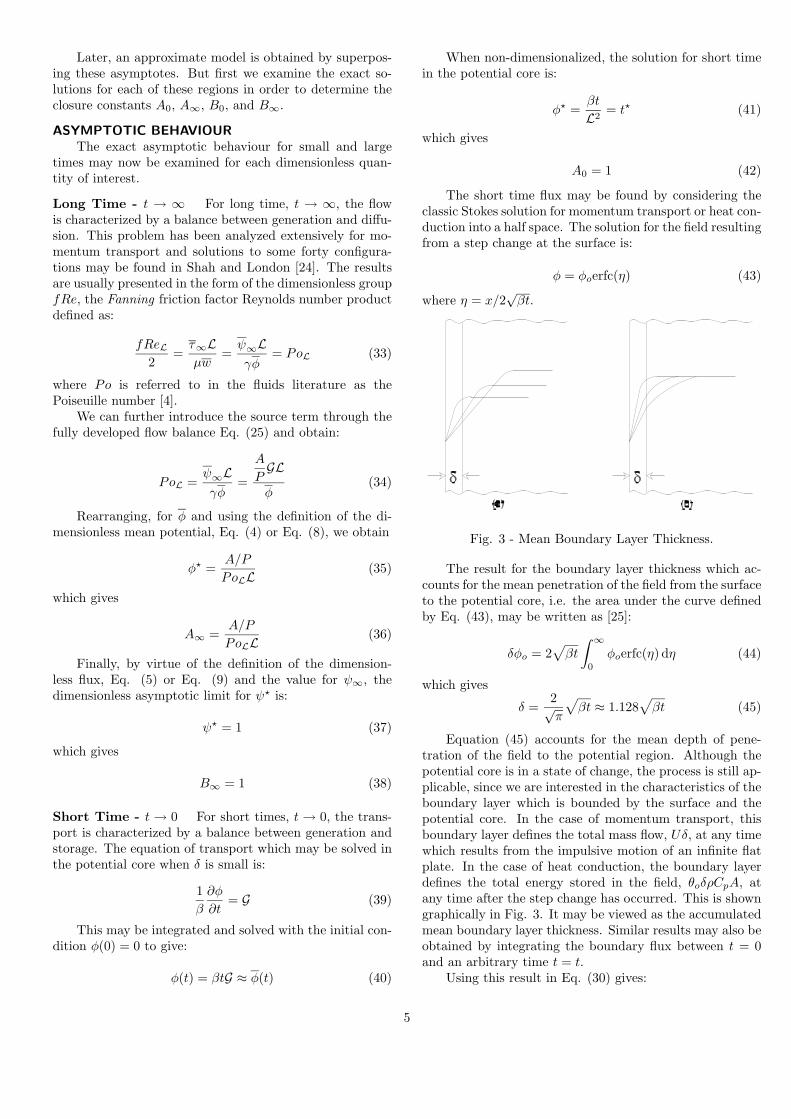
The short time flux may be found by considering theclassic Stokes solution for momentum transport or heat con-duction into a half space. The solution for the field resultingfrom a step change at the surface is:

φ = φoerfc(η) (43)

where η = x/2√

βt.

Fig. 3 - Mean Boundary Layer Thickness.

The result for the boundary layer thickness which ac-counts for the mean penetration of the field from the surfaceto the potential core, i.e. the area under the curve definedby Eq. (43), may be written as [25]:

δφo = 2√

βt

∫ ∞

0

φoerfc(η) dη (44)

which gives

δ =2√π

√

βt ≈ 1.128√

βt (45)

Equation (45) accounts for the mean depth of pene-tration of the field to the potential region. Although thepotential core is in a state of change, the process is still ap-plicable, since we are interested in the characteristics of theboundary layer which is bounded by the surface and thepotential core. In the case of momentum transport, thisboundary layer defines the total mass flow, Uδ, at any timewhich results from the impulsive motion of an infinite flatplate. In the case of heat conduction, the boundary layerdefines the total energy stored in the field, θoδρCpA, atany time after the step change has occurred. This is showngraphically in Fig. 3. It may be viewed as the accumulatedmean boundary layer thickness. Similar results may also beobtained by integrating the boundary flux between t = 0and an arbitrary time t = t.

Using this result in Eq. (30) gives:

5

ψ? =2√π

PLA

√t? (46)

which gives

B0 =2PL√

πA(47)

These exact limits may now be combined in a simplemanner using an asymptotic correlation method.

COMPACT MODELS

Compact models may now be developed using theasymptotic correlation method proposed by Churchill andUsagi [26]. The asymptotic limits may now be combinedto develop a simple compact model for each dimensionlessquantity of interest.

y? = [(y?0)n + (y?

∞)n]1/n (48)

The form for φ? and ψ? is shown in Fig. 4, afterYovanovich [27]. This type of behaviour is characterizedby using a negative value for the fitting parameter n, inEq. (48).

Fig. 4 - Asymptotic Model Development.

The models of interest may now be written in the fol-lowing forms:

φ? =

[

(t?)n +

(A/P

LPoL

)n]1/n

(49)

and

ψ? =

[(2PL√

πA

√t?

)p

+ 1

]1/p

(50)

The values of n and p may now be determined fromcomparisons with data obtained from the exact solutionsto a number of geometries. The fitting parameters may beobtained by either applying Eqs. (49) and (50) at a single

known point in the transition region or by using multiplepoints and minimizing the root mean square error. In thepresent work, the latter method is used to determine thefitting parameters.

Characteristic Length Scale We shall now considerthe various choices for the characteristic length scale L. Thesimplest choice depending on geometry is to use the intrin-sic length scale of the geometry, i.e. L = a for a plane wallof width 2a and cylinder of diameter 2a. However, whendealing with more complex shapes, the choice for momen-tum transport is often the hydraulic diameter defined asL = 4A/P . More recently, Yovanovich and Muzychka [28]and Muzychka and Yovanovich [29] have proposed usingL =

√A with much success in reducing Poiseuille numbers

to a simple function of duct aspect ratio for momentumtransport.

Examination of the proposed compact models suggestsusing L = 4A/P since it simplifies the form of the models.However, L =

√A offers the advantage that the Poiseuille

number is a weak function of shape and can be easily pre-dicted for more complex shapes. The important result ofMuzychka and Yovanovich [29] is that the Poiseuille num-bers may be accurately predicted for the elliptic, rectangu-lar, annular and polygonal shapes using:

fRe√A = 2Po√A =12

√ε(1 + ε)

[

1 − 192ε

π5tanh

( π

2ε

)]

(51)The above expression represents a single term approxi-

mation for the rectangular duct provided 0 < ε ≤ 1, whereε = b/a is the duct aspect ratio. Typical results are given inTables 2 and 3 for the elliptic, rectangular, and polygonalgeometries. Graphical results are provided in Figs. 5 and

6. In the case of the circular annulus ε ≈ (1 − r∗)

π(1 + r∗)where

r∗ = b/a is the radii ratio of the annulus.

Table 2fRe Results for Elliptical and Rectangular

Geometries [24]

fReDhfRe√

A

ε = b/a Rect. Ellip.fReR

fReERect. Ellip.

fReR

fReE

0.01 23.67 19.73 1.200 119.56 111.35 1.0740.05 22.48 19.60 1.147 52.77 49.69 1.0620.10 21.17 19.31 1.096 36.82 35.01 1.0520.20 19.07 18.60 1.025 25.59 24.65 1.0380.30 17.51 17.90 0.978 20.78 20.21 1.0280.40 16.37 17.29 0.947 18.12 17.75 1.0210.50 15.55 16.82 0.924 16.49 16.26 1.0140.60 14.98 16.48 0.909 15.47 15.32 1.0100.70 14.61 16.24 0.900 14.84 14.74 1.0070.80 14.38 16.10 0.893 14.47 14.40 1.0050.90 14.26 16.02 0.890 14.28 14.23 1.0041.00 14.23 16.00 0.889 14.23 14.18 1.004

6

Table 3fRe Results for Polygonal Geometries [24]

N fReDh

fReP

fReCfRe√

A

fReP

fReC

3 13.33 0.833 15.19 1.0714 14.23 0.889 14.23 1.0045 14.73 0.921 14.04 0.9906 15.05 0.941 14.01 0.9887 15.31 0.957 14.05 0.9918 15.41 0.963 14.03 0.9899 15.52 0.970 14.04 0.99010 15.60 0.975 14.06 0.99220 15.88 0.993 14.13 0.996∞ 16 1.000 14.18 1.000

Proposed Compact Models We now consider two pos-sibilities for the characteristic length scale, L, and developcompact models for each parameter of interest.

Hydraulic Diameter, L = 4A/P When the hydraulicdiameter is used as a characteristic length scale Eqs. (49)and (50) become:

φ? =

[

(t?)n +

(1

4PoDh

)n]1/n

(52)

and

ψ? =

[(8√π

√t?

)p

+ 1

]1/p

(53)

Square Root of Area, L =√

A When the square rootof area is used as a characteristic length scale Eqs. (49) and(50) become:

φ? =

[

(t?)n +

(√A/P

Po√A

)n]1/n

(54)

and

ψ? =

[(

2P/√

A√π

√t?

)p

+ 1

]1/p

(55)

The paramater P/√

A is an important geometric scal-ing factor. It is discussed by Yovanovich and Muzychka[28] and Muzychka and Yovanovich [29]. Further, Bejan[30] also showed its importance in a channel flows using hisconstructal theory of nature. The fully developed Poiseuillenumber has the following relationship to this geometric pa-rameter:

Po√A = PoDh

P

4√

A(56)

Fig. 5 - fRe for Elliptic and Rectangular Ducts.

Fig. 6 - fRe for Some Other Duct Shapes.

COMPARISON WITH KNOWN SOLUTIONS

Comparisons will now be made with four known ana-lytical solutions: the plane channel, the circular tube, therectangle, and the circular annulus. Each of these four ge-ometries are closely related. The annulus contains as spe-cial limits the tube and the channel results, and the rectan-gle also contains the channel limit. Further, the rectanglecontains the square duct which is one of the polygonal ductswhich has a strong similarity to the tube and other polyg-onal shapes when appropriately non-dimensionalized, seeTable 3. In the subsequent sections, Eqs. (52) and (53) areused in presenting the model and data comparisons graph-ically.

Parallel Plate Channel The solution for the planechannel of width 2a as found in [7,8,11-13,21] is:

φ(y, t) =Ga2

2

[(

1 − y2

a2

)

−

4

∞∑

n=1

sin(δn)

δ3n

cos(δny/a) exp(−δ2

nβt/a2)

] (57)

7

where

δn =(2n − 1)π

2(58)

Fig. 7 - φ? for the Plane Channel.

Fig. 8 - ψ? for the Plane Channel.

It is of interest to the engineer to obtain the area meanvalue of φ as a function of time. This may be obtained byintegrating the solution across the channel:

φ =1

2a

∫ a

−a

φ(y, t)dy (59)

Evaluating the integral and simplifying yields

φ = Ga2

(

1

3− 2

∞∑

n=1

exp(−δ2

nβt/a2)

δ4n

)

(60)

Finally, the flux may be calculated from:

ψ = −γ∂φ

∂y

∣∣∣∣y=a

(61)

or

ψ = γGa

(

1 − 2∞∑

n=1

exp(−δ2

nβt/a2)

δ2n

)

(62)

Equations (60) and (62) have been used to generatedata for comparisons to the proposed models. Over the

range of 0.0001 < t? < 10, 50-200 terms were used in theseries as required to achieve convergence. The optimal fit-ting parameter for φ? was found to be n = −1.3 with a rootmean square error (RMS) of 6.03 percent. While for ψ? thevalue was found to be p = −6 with a 0.262 percent RMS.Graphical results are shown in Figs. 7 and 8.

Fig. 9 - φ? for the Circular Tube.

Fig. 10 - ψ? for the Circular Tube.

Circular Tube The solution for the circular tube ofdiameter 2a was obtained by Szymanski [6] using the sepa-ration of variables method. The solution is widely discussedin many advanced level fluid texts [1-5] and a heat conduc-tion text [21]. The solution is:

φ(r, t) =Ga2

4

[(

1 − r2

a2

)

−

8

∞∑

n=1

Jo (δnr/a)

δ3nJ1(δn)

exp(−δ2

nβt/a2)

] (63)

where δn are the positive roots of

J0(δn) = 0 (64)

The mean potential may be found by integrating overthe cross-sectional area

8

φ =2

a2

∫ a

0

φ(r, t)rdr (65)

or

φ = Ga2

(

1

8− 4

∞∑

n=1

exp(−δ2

nβt/a2)

δ3n

)

(66)

Finally, the shear stress is found from

ψ = −γ∂φ

∂r

∣∣∣∣r=a

(67)

or

ψ = γGa

(

1

2− 2

∞∑

n=1

exp(−δ2

nβt/a2)

δ2n

)

(68)

Equations (66) and (68) have been used to generatedata for comparisons to the proposed models. Over therange of 0.0001 < t? < 10, 50-200 terms were used in theseries as required to achieve convergence. The optimal fit-ting parameter for φ? was found to be n = −1.2 with anRMS error of 6.94 percent. While for ψ? the value wasfound to be p = −2.8 with an RMS error of 2.72 percent.Graphical results are shown in Figs. 9 and 10.

Rectangular Channel A search of the literature for asolution for the rectangular channel revealed a form in Er-dogan [10]. The solution is quite cumbersome due to thenature of the approach taken to obtain it. The present au-thors have obtained the solution using the integral trans-form method by means of a double finite sine transform[18-20]. The solution for a rectangle having dimensions a, bwith the origin placed in the lower left corner may be writ-ten in the following form:

φ(x, y, t) =4

ab

∞∑

m=1

∞∑

n=1

Amn[1 − exp(−λ2

mnβt)]

λ2mn

∗

sin(mπx/a) sin(nπy/b)

(69)

where

Amn =Gab[(−1)m − 1][(−1)n − 1]

mnπ2(70)

and

λ2

mn =m2π2

a2+

n2π2

b2(71)

The mean potential at any time is obtained from:

φ =1

ab

∫ b

0

∫ a

0

φ(x, y, t)dxdy (72)

which gives:

φ =

4

ab

∞∑

m=1

∞∑

n=1

Amn[1 − exp(−λ2

mnβt)][(−1)m − 1][(−1)n − 1]

mnπ2λ2mn

(73)

Fig. 11 - φ? for the Rectangular Channel.

Fig. 12 - ψ? for the Rectangular Channel.

The mean wall flux is obtained from:

ψ =1

a + b

[∫ b

0

γ∂φ

∂x

∣∣∣∣x=0

dy +

∫ a

0

γ∂φ

∂y

∣∣∣∣y=0

dx

]

(74)

where∫ b

0

γ∂φ

∂x

∣∣∣∣x=0

dy =

4γ

a2

∞∑

m=1

∞∑

n=1

Amnm[1 − exp(−λ2

mnβt)][1 − (−1)n]

nλ2mn

(75)

and∫ a

0

γ∂φ

∂y

∣∣∣∣y=0

dx =

4γ

b2

∞∑

m=1

∞∑

n=1

Amnn[1 − exp(−λ2

mnβt)][1 − (−1)m]

mλ2mn

(76)

Equations (73) and (74) have been used to generatedata for comparisons to the proposed models. Over therange of 0.0001 < t? < 10, 50-200 terms were used in theseries as required to achieve convergence. Values for n andp are shown in Table 4 for various channel aspect ratios.Graphical results are shown in Figs. 11 and 12.

9

Table 4Results for Rectangular Channel

b/a PoDhn RMS p RMS

0 12 -1.2 6.1 -6 1.8

1/20 11.24 -1.2 6.3 -4.5 2.2

1/10 10.58 -1.2 6.1 -4 2.7

1/6 9.85 -1.2 6.4 -3.5 3.3

1/3 8.54 -1.1 6.7 -2.8 4.0

1/2 7.77 -1.1 6.9 -2.5 4.4

1 7.12 -1.1 6.9 -2.4 4.3

Circular Annulus The solution for the circular annu-lus with inner radius b and outer radius a, was obtained byMuller [9] using the separation of variables method. Thesolution which also contains Bessel functions, is much morecomplex than that for the tube. The final solution for thefield is:

φ(r, t) =Ga2

4

[

1 − %2 − (1 − r∗2) ln(1/%)

ln(1/r∗)

]

−

πa2G∞∑

n=1

J0(δn)[J0(%δn)Y0(r∗δn) − Y0(%δn)J0(r

∗δn)]

δ2n[J0(δn) + J0(r∗δn)]

∗

exp(−δ2

nβt/a2)

(77)where r∗ = b/a, % = r/a, and the eigenvalues, δn, are com-puted numerically from

J0(δn)Y0(r∗δn) − J0(r

∗δn)Y0(δn) = 0 (78)

The functions J0(·) and Y0(·) are Bessel functions of thefirst and second kind, respectively, of order zero. They areeasily evaluated using the symbolic math program MapleV9 [31].

The mean potential may be found by integrating overthe cross-sectional area

φ =2

a2 − b2

∫ a

b

φ(r, t)rdr (79)

which gives:

φ =Ga2

4

[

1 − r∗2 − (1 − r∗2)

ln(1/r∗)

]

−

Ga2

(4

1 − r∗2

) ∞∑

n=1

J0(r∗δn) − J0(δn)

δ4n[J0(δn) + J0(r∗δn)]

∗

exp(−δ2

nβt/a2)

(80)

Fig. 13 - φ? for the Circular Annulus.

Fig. 14 - ψ? for the Circular Annulus.

The mean wall flux is obtained from the following ex-pression:

ψ =1

2π(a + b)

[

γ2πb∂φ

∂r

∣∣∣∣r=b

− γ2πa∂φ

∂r

∣∣∣∣r=a

]

(81)

where

γ2πb∂φ

∂r

∣∣∣∣r=b

=πγGa2

2

[((1 − r∗2)

ln(1/r∗)− 2r∗2

)

+

8∞∑

n=1

J0(δn)

δ2n[J0(δn) + J0(r∗δn)]

exp(−δ2

nβt/a2)

] (82)

and

−γ2πa∂φ

∂r

∣∣∣∣r=a

=πγGa2

2

[(

2 − (1 − r∗2)

ln(1/r∗)

)

−

8

∞∑

n=1

J0(r∗δn)

δ2n[J0(δn) + J0(r∗δn)]

exp(−δ2

nβt/a2)

] (83)

The above expression is easily evaluated using the sym-bolic math program Maple V9 [31].

Equations (80) and (81) have been used to generatedata for comparisons to the proposed models. Over the

10

range of 0.0001 < t? < 10, 50-200 terms were used in theseries as required to achieve convergence. Values for n andp are shown in Table 5 for various radii ratios. Graphicalresults are shown in Figs. 13 and 14.

Table 5Results for Circular Annulus

b/a PoDhn RMS p RMS

0 8 -1.2 6.9 -2.8 2.7

0.0001 8.97 -1.2 6.6 -3.3 2.1

0.01 10.01 -1.2 6.4 -4.0 1.3

0.08 11.05 -1.3 6.3 -4.8 0.61

0.20 11.54 -1.3 6.2 -5.6 0.34

0.90 11.99 -1.3 6.0 -6.0 0.24

RESULTS AND DISCUSSION

Examination of the data, shows that the fitting pa-rameter n for the mean potential φ is very nearly constant−1.3 < n < −1.1, with a mean value n = −6/5 for all datasets. However, the fitting parameter p for the mean flux ψvaries with geometry or duct aspect ratio b/a. Values for pfall in the range −6 < p < −2.4, with the largest absolutevalue for the plane channel. The mean value for all datasets examined is p = −4. It is proposed for simplicity, thata single value representing the mean value of n and p, beused for each model. In the case of the mean potential,this incurs a very small error due to the small range of thisparameter. In the case of the mean flux, the RMS errorfor the channel increases to 2.21 percent from 0.26 precent,while for the tube the RMS error increases to 4.26 percentfrom 2.72 precent. On the whole, choosing a constant valueof p provides an accuracy in the range of 2.21 - 7.57 percentRMS for the rectangle, and 2.21-4.26 percent RMS for theannulus.

The proposed models may also be applied to any shapefor which no known solution exists. As can be seen in Eqs.(52-55), the only parameter which must be known aprioriis the steady state Poiseuille number. Since this param-eter has been determined exactly or numerically for someforty shapes [24], the models can be applied to a wide rangeof geometeries. Further, by means of Eq. (51), Poiseuillenumbers for most common shapes may be calculated within10 percent. The effect of aspect ratio on the fitting param-eter was shown to be moderate. The use of a single valueintroduces a small error for the sake of generality. There-fore, the proposed models may be assumed to be universalfor any shape of interest.

SUMMARY AND CONCLUSIONS

Solutions to the transient Poisson equation for the cir-cular tube, plane channel, rectangular channel, and circu-lar annulus were examined. These solutions are used tomodel either unsteady heat conduction due to a uniformheat source or unsteady viscous momentum transport due

to a suddenly imposed pressure gradient. The solutions arein the form of single and double infinite series some of whichrequire numerical solution to the eigenvalues. To facilitatecomputation of mean potential and mean surface flux, sim-ple models have been proposed which allow for rapid deter-mination of these parameters. The models are defined byEqs. (52) and (53) or Eqs. (54) and (55) in conjunctionwith Eq. (51). The fitting parameters for these equationsare:

n = −6/5

p = −4(84)

These models were developed by means of scale analysisand asymptotic analysis of the governing equation. Theproposed models were compared with data generated fromthe exact solutions. Overall agreement between model andtheory is quite good with an RMS error between 2-6 pre-cent for all data examined when a single constant value ofthe correlation parameters was chosen. The models werealso shown to be applicable to any non-circular geometryprovided an exact or approximate value of the steady statePoiseuille number is known for the non-circular geometry.

ACKNOWLEDGMENTS

The authors acknowledge the financial support of theNatural Sciences and Engineering Research Council ofCanada (NSERC) through the Discovery Grants Program.The authors also thank K. Boone, Z. Duan, and M.Bahrami for assistance with the figures.

REFERENCES

[1] Bird, R.B., Stewart, W.E., and Lightfoot, E.N., Trans-

port Phenomena, Wiley, pp. 126-130, 1960.[2] Brodkey, R.S., Phenomena of Fluid Motions, DoverPublishing, pp. 91-95, 1967.[3] Batchelor, G.K., Introduction to Fluid Dynamics, Cam-bridge University Press, pp. 193-195, 1970.[4] White, F.M., Viscous Fluid Flow, McGraw-Hill, 1991.[5] Telionis, D.P., Unsteady Viscous Flows, Springer-Verlag,pp., 1981.[6] Szymanski, P., “Quelques Solutions Exactes des Equa-tions de l’Hydrodyn- amique du Fluide Visqueux dans leCas d’un Tube Cylindrique”, Journal Mathematique Pure

et Appliquee, Vol. 11, p. 67-107, 1932.[7] Rouse, H. (ed.), Advanced Mechanics of Fluids, Wiley,pp. 221-223, 1959.[8] Arpaci, V.S. and Larsen, P., Convection Heat Transfer,Prentice-Hall, p. 73, 1984.[9] Muller, W., “Zum Problem der Anlaufstromung einerFlussigkeit im geraden Rohr mit Kreisring und Kreisquer-schnitt”, ZAMM, Vol. 16, pp. 227-238, 1936.[10] Erdogan, M.E., “On the Flows Produced by SuddenApplication of a Constant Pressure Gradient or by Impul-sive Motion of a Boundary”, International Journal of Non-

Linear Mechanics, Vol. 38, pp. 781-797, 2003.[11] Lamb, H., “A Paradox in Fluid Motion”, Journal of the

London Mathematical Society, Vol. 2, pp. 109-112, 1927.[12] Bromwich, T.J., “An Application of Heaviside’s Meth-ods to Viscous Fluid Motion”, Journal of the London Math-

11

ematical Society, Vol. 5, pp. 10-13, 1930.[13] Carslaw, H.S. and Jaeger, J.C., Operational Methods

in Applied Mathematics, Oxford, pp. 169-170, 1948.[14] Berker, R., Handbuch der Physik, Vol. VIII, Springer-Verlag, 1963.[15] Wang, C.Y., “Exact Solutions of the Unsteady Navier-Stokes Equations”, Applied Mechanics Reviews, Vol. 42,pp. S269-S282, 1989.[16] Wang, C.Y., “Exact Solutions of the Steady StateNavier-Stokes Equations”, Annual Review of Fluid Mechan-

ics, Vol. 23, pp. 159-177, 1991.[17] Erdogan, M.E., “On the Unsteady UnidirectionalFlows Generated by Impulsive Motion of a Boundary orSudden Application of Pressure Gradient”, International

Journal of Non-Linear Mechanics, Vol. 37, pp. 1091-1106,2002.[18] Sneddon, I.N., Fourier Transforms, Dover Publishing,1951.[19] Sneddon, I.N., The Uses of Integral Transforms,McGraw-Hill, 1972.[20] Churchill, R.V., Operational Mathematics, McGraw-Hill, 1972.[21] Carslaw, H.S. and Jaeger, J.C., Conduction of Heat in

Solids, Oxford, pp. 130-131, 204-205, 1959.[22] Thews, G., “Uber die Mathematiische BehandlungPhysiologischer Diffusionsprozesse in Zylinderformigen Ob-jekten,” Acta Biotheoretica, Vol. A10, pp. 105-138, 1953.

[23] Bejan, A. Convection Heat Transfer, Wiley, 1995.[24] Shah, R.K. and London, A.L., Laminar Flow Forced

Convection in Ducts, Academic Press, 1978.[25] Yuan, S.W., Foundations of Fluid Mechanics, Prentice-Hall, pp. 291-293, 1967.[26] Churchill, S. W. and Usagi, R., “A General Expressionfor the Correlation of Rates of Transfer and Other Phenom-ena,” American Institute of Chemical Engineers, Vol. 18,pp. 1121-1128, 1972.[27] Yovanovich, M.M., “Asymptotes and Asymptotic Anal-ysis for Development of Compact Models for Microelectron-ics Cooling”, Keynote Address, Semitherm 2003, San Jose,CA, March 2003.[28] Yovanovich, M.M. and Muzychka, Y.S., “Solutions ofPoisson Equation in Singly and Doubly Connected Pris-matic Bars”, AIAA Paper 97-3880, 1997 National Heat

Transfer Conference, Baltimore, MD, 1997.[29] Muzychka, Y.S. and Yovanovich, M.M., “Laminar FlowFriction and Heat Transfer in Non-Cicular Ducts - Part IHydrodynamic Problem”, Compact Heat Exchangers - A

Festschrift on the 60th Birthday of Ramesh K. Shah, (eds.)G.P. Celata, B. Thonon, A. Bontemps, and S. Kandlikar,Edizioni ETS, pp. 123-130, 2002.[30] Bejan, A., Shape and Structure: From Engineering to

Nature, Cambridge, 2000.[31] Maple V9, Waterloo Maple Software, 2003.

12