comp9334 capacity planning for computer systems and networkscs9334/17s1/week02-noblocking.pdf ·...
TRANSCRIPT

COMP9334 1
COMP9334Capacity Planning for Computer Systems and Networks
Week 2: Operational Analysis andWorkload Characterisation

S1,2017 COMP9334 2
Last lecture
• Modelling of computer systems using Queueing Networks• Open networks• Closed networks

S1,2017 COMP9334 3
Open networks
A transaction may visit the CPU and disk multiple times.An open network is characterised by external transactions.
Example: The server has a CPU and a disk. Open queueing network
External arrivals
Workload intensity specified by arrival rate
Unbounded number of customers in the system
In equilibrium, flow in = flow out) throughput = arrival rate
Page 26

S1,2017 COMP9334 4
Closed queuing networks
Closed queueing networks model• Running batch jobs overnight• Once a job has completed, a new job starts.Good performance means high throughput. #jobs in the system = multi-programming level
Database server for batch jobs
Running batch jobs overnight
E.g. producing managerial reports
Assume once a job has completed, a new job starts
Maintain constant number of customers in the system
A closed queueing networkPage 25
S1,2017 COMP9334 5
This lecture
• The basic performance metrics• Response time, Throughput, Utilisation etc.
• Operational analysis• Fundamental Laws relating the basic performance metrics• Bottleneck and performance analysis
• Workload characterisation• Poisson process and its properties
S1,2017 COMP9334 6
Operational analysis (OA)
• “Operational”• Collect performance data during day-to-day operation
• Operation laws• Applications:
• Use the data for building queueing network models• Perform bottleneck analysis• Perform modification analysis
• iostat
S1,2017 COMP9334 7

S1,2017 COMP9334 8
Single-queue example (1)
In an observational period of T, server busy for time BA requests arrived, C jobs completed
A, B and C are basic measurements
Deductions: Arrival rate l = A/TOutput rate X = C/TUtilisation U = B/TMean service time per completed request = B/C
server
#requests = A #requests = C
B
Motivating example
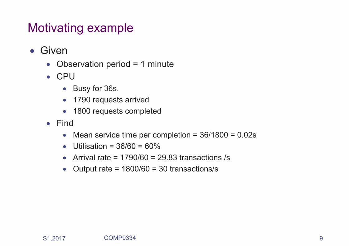
• Given• Observation period = 1 minute• CPU
• Busy for 36s.• 1790 requests arrived• 1800 requests completed
• Find• Mean service time per completion = 36/1800 = 0.02s• Utilisation = 36/60 = 60%• Arrival rate = 1790/60 = 29.83 transactions /s• Output rate = 1800/60 = 30 transactions/s
S1,2017 COMP9334 9

S1,2017 COMP9334 10
Utilisation law
• The operational quantities are inter-related• Consider
• Utilisation U = B / T• Mean service time per completion S = B / C• Output rate X = C / T
• Utilisation law – Can you relate U, S and X? • U = S X
• Utilisation law is an example of operational law.

S1,2017 COMP9334 11
Application of OA
• Don’t have to measure every operational quantities• Measure B to deduce U - don’t have to measure U
• Consistency checks• If U ¹ S X, something is wrong
• Operational laws can be used for performance analysis• Bottleneck analysis (today)• Mean value analysis (Later in the course)

S1,2017 COMP9334 12
Equilibrium assumption
• OA makes the assumption that• C = A • Or at least C » A
• This means that • The devices and system are in equilibrium
• Arrival rate of requests to a device = Output rate of requests for that device = Throughput of the device
• The above statement also applies to the system, i.e. replace the word “device” by “system”

S1,2017 COMP9334 13
OA for Queueing Networks (QNs)
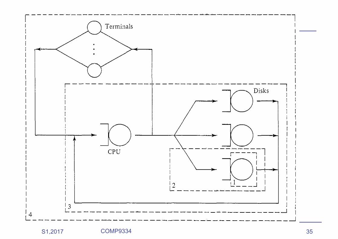
The computersystem has Kdevices, labelledas 1,…,K.
The conventionis to add anadditional device 0 torepresent theoutside world.

S1,2017 COMP9334 14
OA for QNs (cont’d)
• We measure the basic operational quantities for each device (or other equivalent quantities) over a time of T• A(j) = Number of arrivals at device j• B(j) = Busy time for device j• C(j) = Number of completed jobs for device j
• In addition, we have• A(0) = Number of arrivals for the system• C(0) = Number of completions for the system
• Question: What is the relationship between A(0) and C(0) for a closed QNs?
S1,2017 COMP9334 15
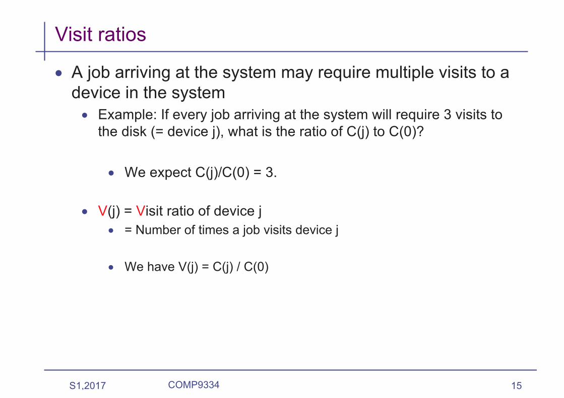
Visit ratios
• A job arriving at the system may require multiple visits to adevice in the system• Example: If every job arriving at the system will require 3 visits to
the disk (= device j), what is the ratio of C(j) to C(0)?
• We expect C(j)/C(0) = 3.
• V(j) = Visit ratio of device j• = Number of times a job visits device j
• We have V(j) = C(j) / C(0)

S1,2017 COMP9334 16
Forced Flow Law
The forced flow law is
Since

S1,2017 COMP9334 17
Service time versus service demand
• Ex: A job requires two disk accesses to be completed. One disk access takes 20ms and the other takes 30ms.
• Service time = the amount of processing time required per visit to the device • The quantities “20ms” and “30ms” are the individual service times.
• D(j) = Service demand of a job at device j is the total service time required by that job• The service demand for this job = 20ms + 30 ms = 50ms

S1,2017 COMP9334 18
Service demand
• Service demand can be expressed in two different ways• Ex: A job requires two disk accesses to be completed. One
disk access takes 20ms and the other takes 30ms.• D(j) = 50ms. • What are V(j) and S(j)?
• Recall that S(j) = mean service time of device j • V(j) = 2. S(j) = 25ms.
• Service demand D(j) = V(j) S(j)
S1,2017 COMP9334 19
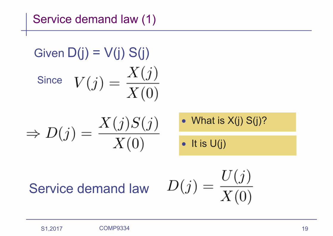
Service demand law (1)
• It is U(j)
Given D(j) = V(j) S(j)
Since
Service demand law
• What is X(j) S(j)?

S1,2017 COMP9334 20
Service demand law (2)
• Service demand law D(j) = U(j) / X(0)• You can determine service demand without knowing the visit ratio• Over measurement period T, if you find
• B(j) = Busy time of device j • C(0) = Number of requests completed
• You’ve enough information to find D(j)
• The importance of service demand• You will see that service demand is a fundamental quantity you
need to determine the performance of a queueing network• You will use service demand to determine system bottleneck today

S1,2017 COMP9334 21
Server example exercise
Measurement time = 1 hr
# I/O/s Utilisation
Disk 1 32 0.30
Disk 2 36 0.41
Disk 3 50 0.54
CPU 0.35
Total # jobs=13680
What is the service time of Disk 2?What is the service demand of Disk 2?What is its visit ratio?
S1,2017 COMP9334 22
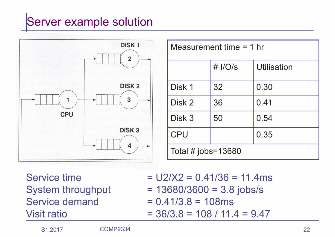
Server example solution
Measurement time = 1 hr
# I/O/s Utilisation
Disk 1 32 0.30
Disk 2 36 0.41
Disk 3 50 0.54
CPU 0.35
Total # jobs=13680
Service time = U2/X2 = 0.41/36 = 11.4msSystem throughput = 13680/3600 = 3.8 jobs/sService demand = 0.41/3.8 = 108msVisit ratio = 36/3.8 = 108 / 11.4 = 9.47
S1,2017 COMP9334 23
Little’s law (1)
• Due to J.C. Little in 1961• A few different forms
• The original form is based on stochastic models• An important result which is non-trivial
• All the other operational laws are easy to derive, but Little’s Law’s derivation is more elaborate.
• Consider a single-server device• Navg = Average number of jobs in the device
• When we count the number of jobs in a device, we include the one being served and those in the queue waiting for service

S1,2017 COMP9334 24
Little’s Law (2)
• X = Throughput of the device• Ravg = Average response time of the jobs• Navg = Average number of jobs in the device • Little’s Law (for OA) says that
Navg = X * RavgWe will argue the validity of Little’s Law using a simple
example.

S1,2017 COMP9334 25
Job index Arrival time Service time Departure time1 2 2 42 6 4 103 8 4 144 9 3 17
2
3
1 time
2 4 6 10 14 17
4
1
2
3
Consider the single sever queue example from Week 1
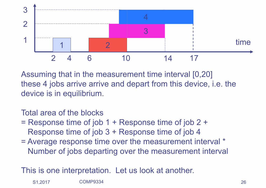
Let us use blocks of height 1 to show the time span of the jobs, i.e. width of each block = response time of the job
2
3
1 time
2 4 6 10 14 17
4
1
2
3
Assuming that in the measurement time interval [0,20] these 4 jobs arrive arrive and depart from this device, i.e. the device is in equilibrium.
Total area of the blocks = Response time of job 1 + Response time of job 2 +
Response time of job 3 + Response time of job 4= Average response time over the measurement interval *
Number of jobs departing over the measurement interval
This is one interpretation. Let us look at another. S1,2017 COMP9334 26

2
3
1 time
2 4 6 10 14 17
4
1
2
3
2 31 4 time
2 4 6 10 14 17
3 4
4
1
2
3
Let us assume these blocks are “plastic” and let them fall to the ground. Like this.
There is an interpretation of the height of the graph. S1,2017 COMP9334 27

Job index Arrival time Service time
1 2 22 6 43 8 44 9 3
2 31 42 4 6 10 14 17
3 4
4
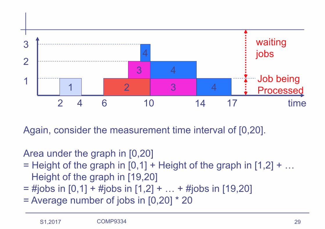
Interpretation: Height of the graph = number of jobs in the deviceE.g. Number of jobs in [9,10] = 3E.g. Number of jobs in [11,12] = 2 etc.
1
2
3
time
waiting jobs
Job being Processed
S1,2017 COMP9334 28
S1,2017 COMP9334 29
Again, consider the measurement time interval of [0,20].
Area under the graph in [0,20]= Height of the graph in [0,1] + Height of the graph in [1,2] + …
Height of the graph in [19,20]= #jobs in [0,1] + #jobs in [1,2] + … + #jobs in [19,20]= Average number of jobs in [0,20] * 20
2 31 42 4 6 10 14 17
3 4
4
1
2
3
time
waiting jobs
Job being Processed

Area = Average number of jobs in [0,T] * T
2 31 42 4 6 10 14 17
3 4
4
1
2
3
time
waiting jobs
Job being Processed
2
3
1 time
2 4 6 10 14 17
4
1
2
3
Area = Average response time over [0,T] * Number of jobs leaving in [0,T]
S1,2017 COMP9334 30

S1,2017 COMP9334 31
Area = Average response time of all jobs * Number of jobs leaving in [0,T] (Interpretation #1)
= Average number of jobs in [0,T] * T (Interpretation #2)
Since Number of jobs leaving in [0,T] / T = Device throughput in [0,T]
We have Little’s Law.
Average number of jobs in [0,T]= Average response time of all jobs * Device throughput in [0,T]
Deriving Little’s Law

Using Little’s Law (1)
• A device consists of a server and a queue• The device completes on average 8 requests per second• On average, there are 3.2 requests in the device • What is the response time of the device?
S1,2017 COMP9334 32
serverqueue
• Mean throughput X = 8 requests/s• Mean number of requests Navg = 3.2 requests • By Little’s Law, average response time = Navg/X = 3.2 / 8 =
0.8 s

Intuition of Little’s Law
• Little’s Law• Mean #jobs = Mean response time * Mean throughput
• If # jobs in the device ⬆ , then response time ⬆• And vice versa
S1,2017 COMP9334 33
S1,2017 COMP9334 34
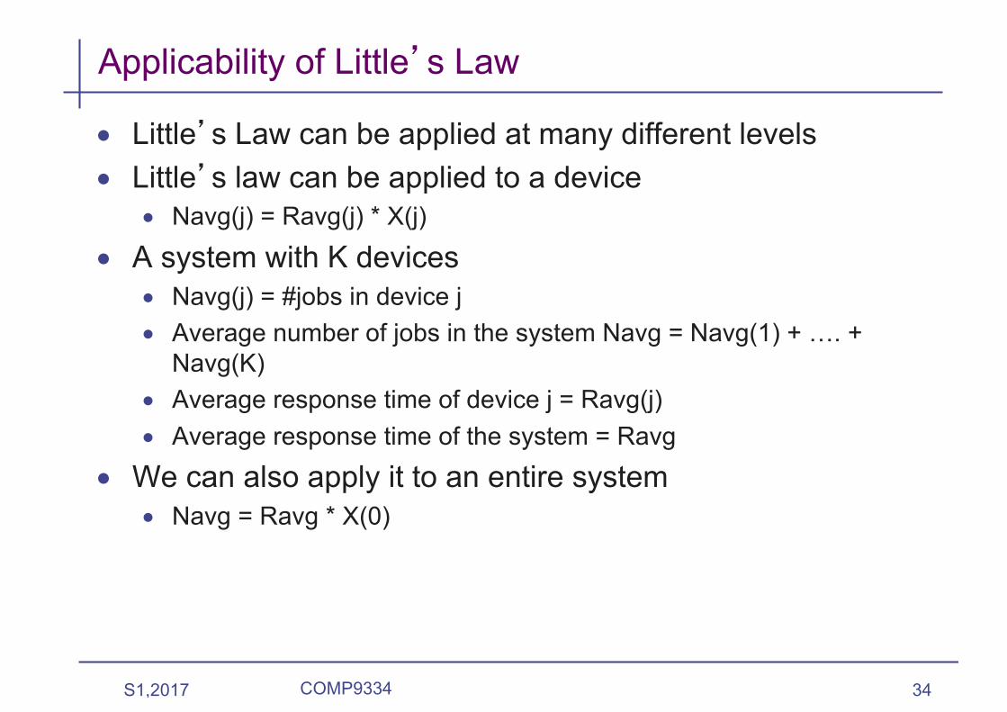
Applicability of Little’s Law
• Little’s Law can be applied at many different levels• Little’s law can be applied to a device
• Navg(j) = Ravg(j) * X(j)• A system with K devices
• Navg(j) = #jobs in device j• Average number of jobs in the system Navg = Navg(1) + …. +
Navg(K)• Average response time of device j = Ravg(j)• Average response time of the system = Ravg
• We can also apply it to an entire system• Navg = Ravg * X(0)
S1,2017 COMP9334 35
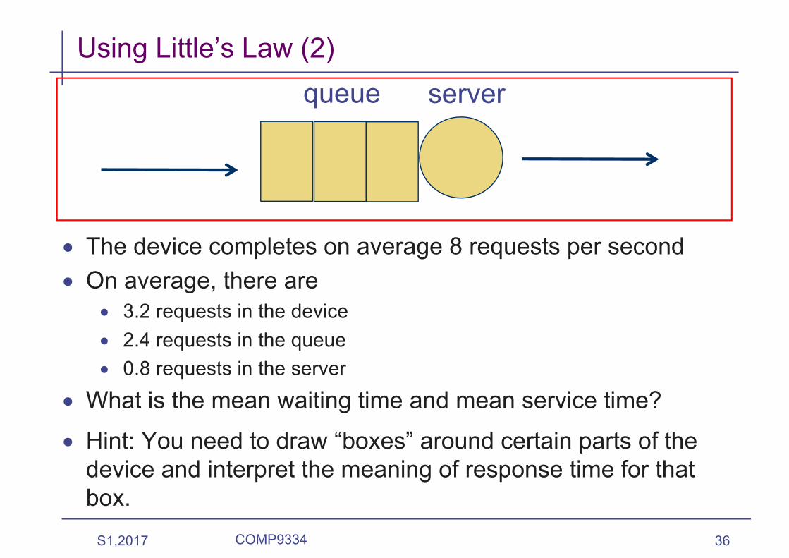
Using Little’s Law (2)
• The device completes on average 8 requests per second• On average, there are
• 3.2 requests in the device• 2.4 requests in the queue• 0.8 requests in the server
• What is the mean waiting time and mean service time?
S1,2017 COMP9334 36
serverqueue
• Hint: You need to draw “boxes” around certain parts of the device and interpret the meaning of response time for that box.
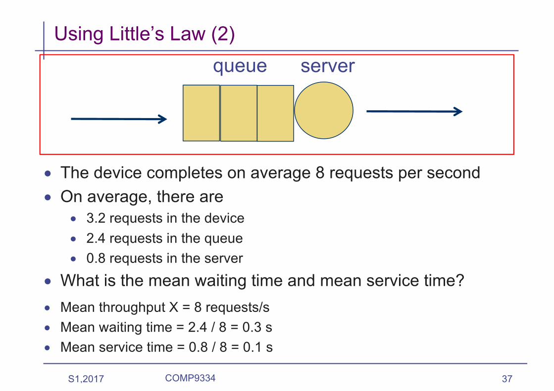
Using Little’s Law (2)
• The device completes on average 8 requests per second• On average, there are
• 3.2 requests in the device• 2.4 requests in the queue• 0.8 requests in the server
• What is the mean waiting time and mean service time?
S1,2017 COMP9334 37
serverqueue
• Mean throughput X = 8 requests/s• Mean waiting time = 2.4 / 8 = 0.3 s• Mean service time = 0.8 / 8 = 0.1 s

S1,2017 COMP9334 38
Interactive systems
M users Each user sends a job tothe system
The system sends theresults to the user.
The user after a thinkingtime, sends another job tothe system.- Thinking time = timespent by the user
An interactive system isan example of closedsystem.
results jobs

S1,2017 COMP9334 39
Interactive systems (Time line)
results jobs
User 1
User 1 sends a job to the computer system
The time the job spends in the computer
system
Results are returned to
the user
Thinking timetime

S1,2017 COMP9334 40
Interactive system (1)
• M interactive clients• Z = mean thinking time• R = mean response time
of the computer system• X0 = throughput

S1,2017 COMP9334 41
Interactive system (2)
• Mavg = mean # interactive clients
• Z = mean thinking time• X0 = throughput• Apply Little’s Law to
the interactive part, we have Mavg = Z * X0

S1,2017 COMP9334 42
Interactive system (3)
• Navg = average # clients in the computer system
• R = mean response time at the computer system
• X0 = throughput• Apply Little’s Law to the
computer system, we have Navg = R * X0

S1,2017 COMP9334 43
Interactive system (4)
• Mavg = X0 * Z• Navg = X0 * R• The system is closed, the
total number of users M is a constant, we have
• M = Mavg + Navg• Therefore, • M = X0 * (Z+R)

S1,2017 COMP9334 44
The operational laws
• These are the operational laws• Utilisation law U(j) = X(j) S(j) • Forced flow law X(j) = V(j) X(0)• Service demand law D(j) = V(j) S(j) = U(j) / X(0)• Little’s law N = X R • Interactive response time M = X(0) (R+Z)
• Applications• Mean value analysis (later in the course)• Bottleneck analysis• Modification analysis

S1,2017 COMP9334 45
Bottleneck analysis - motivation
D(j) Utilisation
Disk 1 79ms 0.30
Disk 2 108ms 0.41
Disk 3 142ms 0.54
CPU 92ms 0.35
Service demand law: D(j) = U(j) / X(0)==> U(j) = D(j) X(0)Utilisation increases with increasing throughput and service demand

Utilisation vs. throughput plot U(j) = D(j) X(0)
Observation: For all system throughput: Utilisation of Disk 3 > Utilisation of Disk 2 > Utilisation of CPU > Utilisation of Disk 1
Disk 3
Disk 2
Disk 1
CPU
What determinesthis order?
S1,2017 COMP9334 46

S1,2017 COMP9334 47
Bottleneck analysis
• Recall that utilisation is the busy time of a device divided by measurement time• What is the maximum value of utilisation?
• Based on the example on the previous slide, which device will reach the maximum utilisation first?

S1,2017 COMP9334 48
Bottleneck (1)
• Disk 3 has the highest service demand• It is the bottleneck of the whole system
Operational law:
Utilisation limit: }

S1,2017 COMP9334 49
Bottleneck (2)
Should hold for all K devices in the system
Bottleneck throughput islimited by the maximumservice demand

S1,2017 COMP9334 50
Bottleneck exercise
D(j) Utilisation
Disk 1 79ms 0.30
Disk 2 108ms 0.41
Disk 3 142ms 0.54
CPU 92ms 0.35
The maximum system throughput is 1 / 0.142 = 7.04 jobs/s.What if we upgrade Disk 3 by a new disk that is 2 times faster,which device will be the bottleneck after the upgrade? Youcan assume that service time is inversely proportional to diskspeed.

S1,2017 COMP9334 51
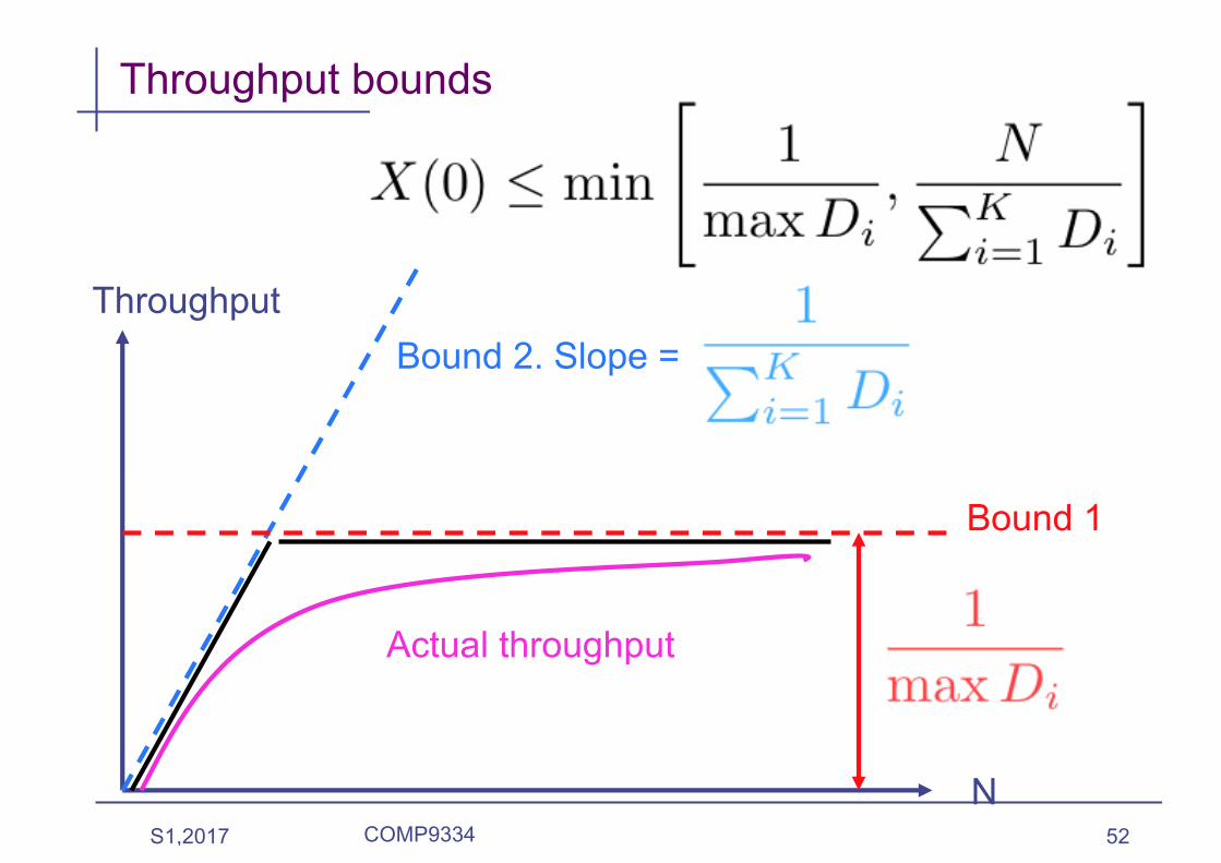
Another throughput bound• Little’s law
Previously, we have
Therefore:
S1,2017 COMP9334 52
Throughput bounds
Throughput
N
Bound 1
Bound 2. Slope =
Actual throughput

S1,2017 COMP9334 53
Bottleneck analysis
• Simple to use• Needs only utilisation of various components
• Assumes service demand is load independent
S1,2017 COMP9334 54
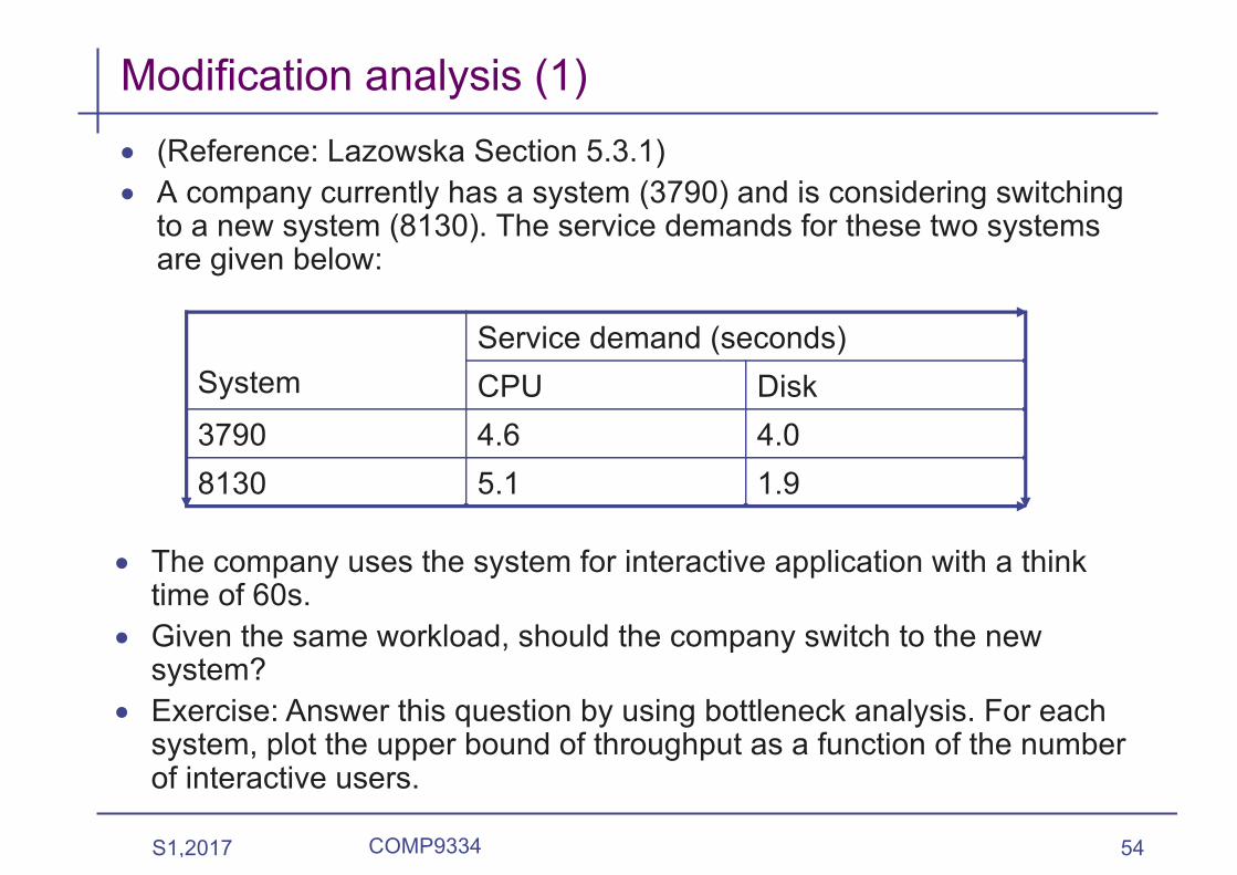
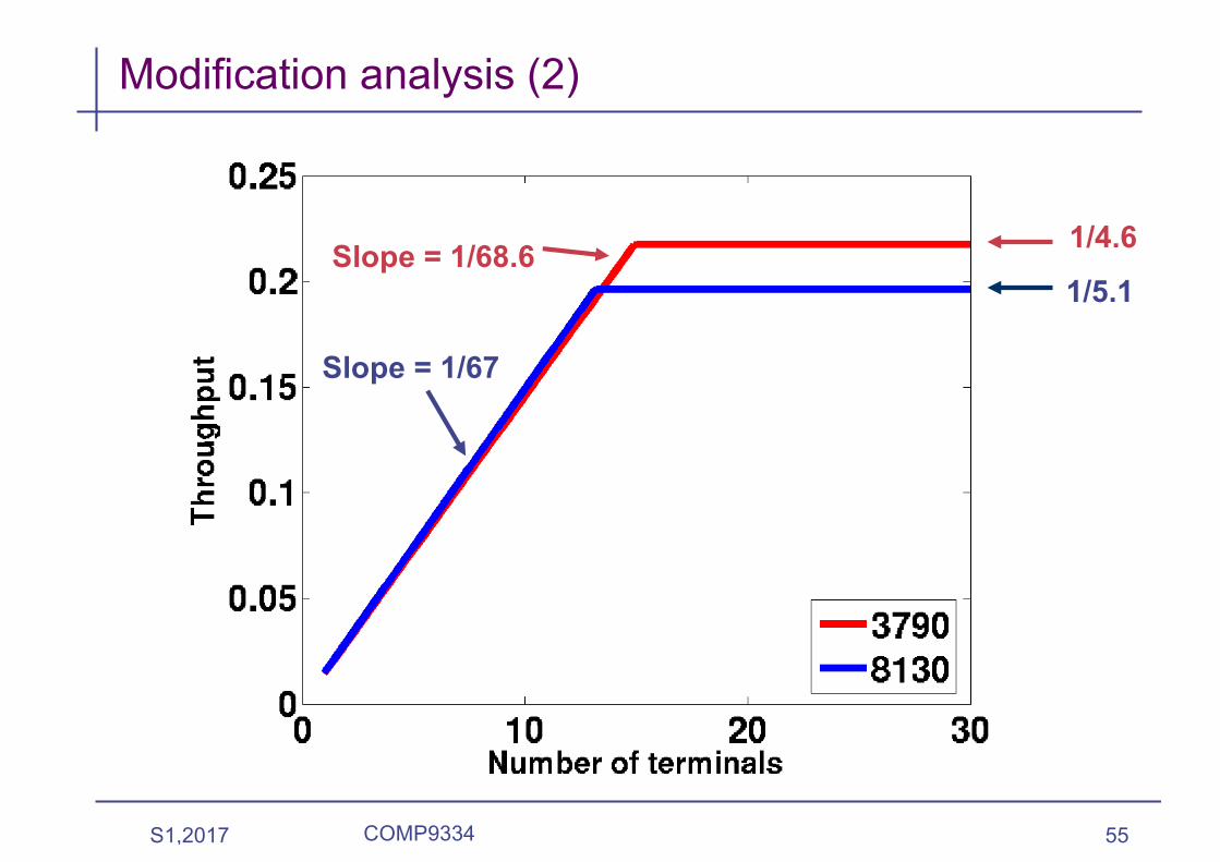
Modification analysis (1)• (Reference: Lazowska Section 5.3.1)• A company currently has a system (3790) and is considering switching
to a new system (8130). The service demands for these two systems are given below:
SystemService demand (seconds)CPU Disk
3790 4.6 4.08130 5.1 1.9
• The company uses the system for interactive application with a think time of 60s.
• Given the same workload, should the company switch to the new system?
• Exercise: Answer this question by using bottleneck analysis. For each system, plot the upper bound of throughput as a function of the number of interactive users.
S1,2017 COMP9334 55
Modification analysis (2)
Slope = 1/67
Slope = 1/68.6 1/4.61/5.1

S1,2017 COMP9334 56
Operational analysis
• These are the operational laws• Utilisation law U(j) = X(j) S • Forced flow law X(j) = V(j) X(0)• Service demand law D(j) = V(j) S(j) = U(j) / X(0)• Little’s law N = X R • Interactive response time M = X(0) (R+Z)
• Operational analysis allows you to bound the system performance but it does NOT allow you to find the throughput and response time of a system
• To order to find the throughput and response time, we need to use queueing analysis
• To order to use queueing analysis, we need to specify the workload

S1,2017 COMP9334 57
Workload analysis
• Performance depends on workload• When we look at performance bound earlier, the bounds depend
on number of users and service demand• Queue response time depends on the job arrival rate and job
service time
• One way of specifying workload is to use probability distribution.
• We will look at a well-known arrival process called Poisson process today.
• We will first begin by looking at exponential distribution.

S1,2017 COMP9334 58
Exponential distribution (1)
• A continuous random variable is exponentially distributed with rate l if it has probability density function
Probability that x £ X £ x + dx is
f(x) dx = l exp(- lx) dx

S1,2017 COMP9334 59
Exponential distribution - cumulative distribution
• The cumulative distribution function F(x) = Prob(X £ x) is:
What is Prob(X ³ x)?
S1,2017 COMP9334 60
Arrival process
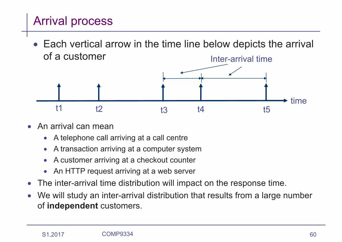
• Each vertical arrow in the time line below depicts the arrival of a customer
• An arrival can mean• A telephone call arriving at a call centre• A transaction arriving at a computer system• A customer arriving at a checkout counter• An HTTP request arriving at a web server
• The inter-arrival time distribution will impact on the response time. • We will study an inter-arrival distribution that results from a large number
of independent customers.
timet1 t2 t3 t4 t5
Inter-arrival time

S1,2017 COMP9334 61
Many independent arrivals (1)• Assume there is a large pool of N customers• Within a time period of d (d is a small time period), there is a probability
of pd that a customer will make a request (which gives rise to an arrival)
• Assuming the probability that each customer makes a request is independent, the probability that a customer arrives in time period d is Npd
• If a customer arrives at time 0, what is the probability that the next customer does not arrive before time t
time0 t
No arrival!
S1,2017 COMP9334 62
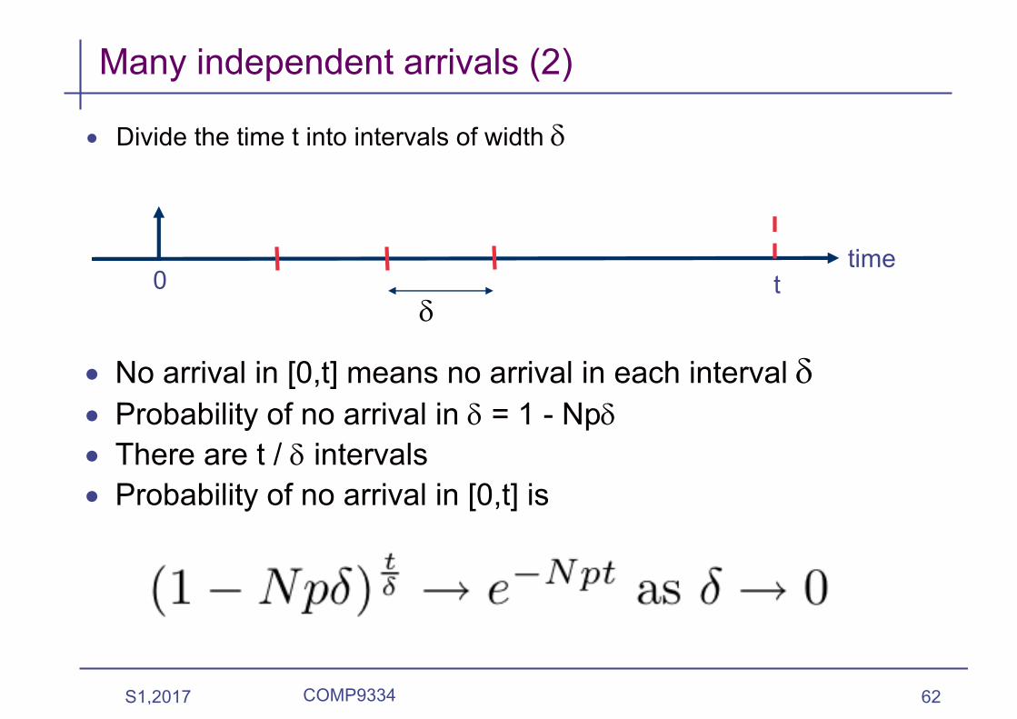
Many independent arrivals (2)
• Divide the time t into intervals of width d
time0 t
d
• No arrival in [0,t] means no arrival in each interval d• Probability of no arrival in d = 1 - Npd• There are t / d intervals• Probability of no arrival in [0,t] is

S1,2017 COMP9334 63
Exponential inter-arrival time
• We have showed that the probability that there is no arrival in [0,t] is exp(- N p t)
• Since we assume that there is an arrival at time 0, this means
Probability(inter-arrival time > t) = exp(- N p t)
• This means Probability(inter-arrival time £ t) = 1 - exp(- N p t)
• What this shows is the inter-arrival time distribution for independent arrival is exponentially distributed
• Define: l = Np• l is the mean arrival rate of customers

Two different methods to describe arrivals
Method 1: Continuous probability distribution of inter-arrival time
S1,2017 COMP9334 64
time
Inter-arrival time

Two different methods to describe arrivals
S1,2017 COMP9334 65
Method 2: Use a fixed time interval (say t), and count the number of arrivals within t.
time
5 arrivals in t 8 arrivals in t 6 arrivals in t
• The number of arrivals in t is random• The number of arrivals must be an non-negative integer• We need a discrete probability distribution:
• Prob[#arrivals in t = 0] • Prob[#arrivals in t = 1] • etc.

S1,2017 COMP9334 66
Poisson process (1)
• Definition: An arrival process is Poisson with parameter l if the probability that n customer arrive in any time interval tis
Example:Example:l= 5 and t = 1
Note: Poisson is adiscrete probabilitydistribution.
S1,2017 COMP9334 67
Poisson process (2)
• Theorem: An exponential inter-arrival time distribution with parameter l gives rise to a Poisson arrival process with parameter l
• How can you prove this theorem?• A possible method is to divide an interval t into small time intervals
of width d. A finite d will give a binomial distribution and with d è 0, we get a Poisson distribution.
S1,2017 COMP9334 68
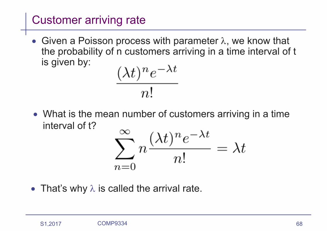
Customer arriving rate
• Given a Poisson process with parameter l, we know that the probability of n customers arriving in a time interval of t is given by:
• What is the mean number of customers arriving in a time interval of t?
• That’s why l is called the arrival rate.

S1,2017 COMP9334 69
Customer inter-arrival time
• You can also show that if the inter-arrival time distribution is exponential with parameter l, then the mean inter-arrival time is 1/l
• Quite nicely, we have Mean arrival rate = 1 / mean inter-arrival time
S1,2017 COMP9334 70
Application of Poisson process
• Poisson process has been used to model the arrival of telephone calls to a telephone exchange successfully
• Queueing networks with Poisson arrival is tractable• We will see that in the next few weeks.
• Beware that not all arrival processes are Poisson! Many arrival processes we see in the Internet today are not Poisson. We will see that later.

S1,2017 COMP9334 71
References• Operational analysis
• Lazowska et al, Quantitative System Performance, Prentice Hall, 1984. (Classic text on performance analysis. Now out of print but can be download from http://www.cs.washington.edu/homes/lazowska/qsp/• Chapters 3 and 5 (For Chapter 5, up to Section 5.3 only)
• Alternative 1: You can read Menasce et al, “Performance by design”, Chapter 3. Note that Menasce doesn’t cover certain aspects of performance bounds. So, you will also need to read Sections 5.1-5.3 of Lazowska.
• Alternative 2: You can read Harcol-Balter, Chapters 6 and 7. The treatment is more rigorous. You can gross over the discussion mentioning ergodicity.
• Little’s Law (Optional)• I presented an intuitive “proof”. A more formal proof of this well known Law is
in Bertsekas and Gallager, “Data Networks”, Section 3.2
• Tutorial exercises based on this week’s lecture are available from course web site• We will discuss the questions in next week’s tutorial time