chapter 7: channel capacity - uic computer science · · 2015-11-13chapter 7: channel capacity...
TRANSCRIPT

University of Illinois at Chicago ECE 534, Fall 2009, Natasha DevroyeUniversity of Illinois at Chicago ECE 534, Fall 2009, Natasha Devroye
Chapter 7: Channel capacity
University of Illinois at Chicago ECE 534, Fall 2009, Natasha Devroye
Chapter 7 outline
• Definition and examples of channel capacity
• Symmetric channels
• Channel capacity properties
• Definitions and jointly typical sequences
• Channel coding theorem: achievability and converse
• Hamming codes
• Channels with feedback
• Source-channel separation theorem

Generic communication block diagram
Source Encoder Channel Decoder Destination
Noise
SourceSource
coderChannel
Source
decoderDestination
Noise
Channel
coder
Channel
decoder
Encoder Decoder
Remove redundancy
Controlled adding of redundancy
Decode signals, detect/correct errors
Restore source
University of Illinois at Chicago ECE 534, Fall 2009, Natasha Devroye
Communication system
Source Encoder Channel Decoder Destination
Noise
Source Encoder Channel Decoder Destination
MessageEstimate of message
University of Illinois at Chicago ECE 534, Fall 2009, Natasha Devroye
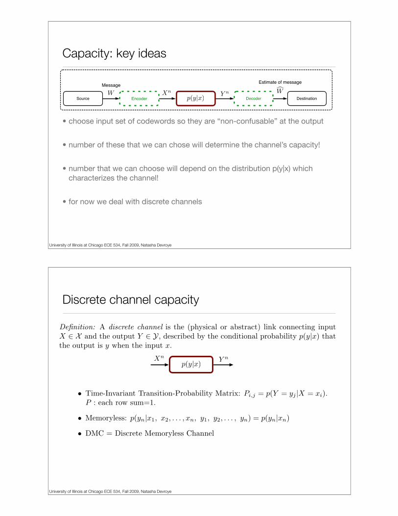
Capacity: key ideas
• choose input set of codewords so they are “non-confusable” at the output
• number of these that we can chose will determine the channel’s capacity!
• number that we can choose will depend on the distribution p(y|x) which characterizes the channel!
• for now we deal with discrete channels
Source Encoder Channel Decoder Destination
MessageEstimate of message
University of Illinois at Chicago ECE 534, Fall 2009, Natasha Devroye
Discrete channel capacity
Channel
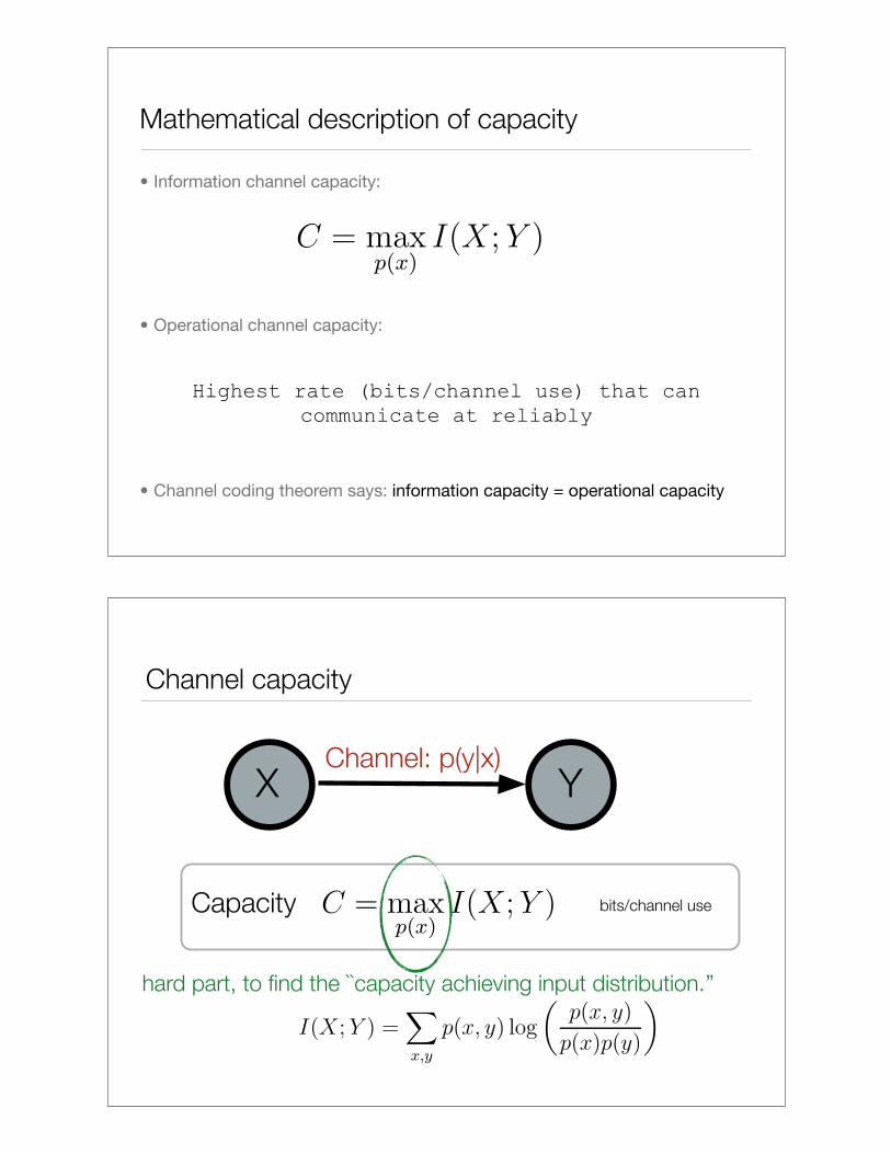
Mathematical description of capacity
• Information channel capacity:
• Channel coding theorem says: information capacity = operational capacity
Pe =n!
i=m+1
"n
i
#f i (1! f)n!i
C = maxp(x)
I(X; Y )
C =1
2log2(1 + |h|2P/PN)
C =
$%
&
12 log2(1 + |h|2P/PN)
Eh
'12 log2(1 + |h|2P/PN)
(
C =
$%
&
maxQ:Tr(Q)=P12 log2
))IMR + HQH†))
maxQ:Tr(Q)=P EH
'12 log2
))IMR + HQH†))(
Y = HX + N
X = H!1U + N
"Y = H(H!1U) + N
= U + N
C =1
2log2(1 + P/N)
R2 # I(Y2; X2|X1)
Let Z = (Y1, Y2,X1,X2,V1,V2, W ) be distributed as:
P (w)$ P (m1!|w)P (m1"|w)P (x1|m1!, m1", w)
$ P (m"1!|m1!, w)P (m"
1"|m1", w)P (m2!|v1, w)P (m2"|v1, w)
$ P (x2|m2!, m2",m", w)P (y1|x1,x2)P (y2|x1,x2)
1
• Operational channel capacity:
Highest rate (bits/channel use) that can
communicate at reliably
Capacity bits/channel useC = maxp(x)
I(X; Y )
1
I(X; Y ) =!
x,y
p(x, y) log
"
p(x, y)
p(x)p(y)
#
B = B1 + B2
! = ", #
(R1!, R1", R2!, R2")
6
X YChannel: p(y|x)
Channel capacity
hard part, to find the ``capacity achieving input distribution.’’
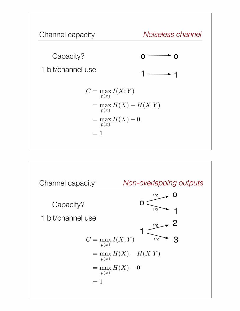
Noiseless channel
o o
1 1
Capacity?
1 bit/channel use
Channel capacity
C = maxp(x)
I(X;Y )
= maxp(x)
H(X)!H(X|Y )
= maxp(x)
H(X)! 0
= 1
o
o
1
1
2
3
1/2
1/2
1/2
1/2
Non-overlapping outputs
Capacity?
1 bit/channel use
Channel capacity
C = maxp(x)
I(X;Y )
= maxp(x)
H(X)!H(X|Y )
= maxp(x)
H(X)! 0
= 1
X
YZ
.
W
V
U
T
A
S
H
G
F
E
DC
JK
LMNOP
B
QR
I
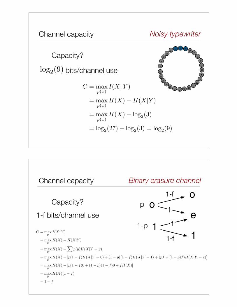
Noisy typewriter
Capacity?
Channel capacity
C = maxp(x)
I(X;Y )
= maxp(x)
H(X)!H(X|Y )
= maxp(x)
H(X)! log2(3)
= log2(27)! log2(3) = log2(9)
bits/channel use
C = maxp(x)
I(X;Y )
= maxp(x)
H(X)!H(X|Y )
= maxp(x)
H(X)! log2(3)
= log2(27)! log2(3) = log2(9)
o
o
e
11
f
f
1-f
1-f
Binary erasure channel
Capacity?
1-f bits/channel use
Channel capacity
p
1-p

o o
1 1
f
f
1-f
1-f
p(y=0|x=0) = p(y=1|x=1)=1-f
p(y=1|x=0) = p(y=0|x=1)=f
Conditional distributionsCapacity?
1-H(f) bits/channel use
Binary symmetric channelChannel capacity
[Cover+Thomas pg.187]
Transition probability matrixReview Examples of Channel Channel Capacity Jointly Typical Sequences
Binary Channels
Binary Symmetric Channel: X = {0, 1} and Y = {0, 1}
X
1
0
1
0
Y
!1 ! f ff 1 ! f
"
Binary Erasure Channel: X = {0, 1} and Y = {0, ?, 1}
1
?X Y
0
1
0
!1 ! f f 00 f 1 ! f
"
Z channel: X = {0, 1} and Y = {0, 1}
X
1
0
1
0
Y
!1 0f 1 ! f
"
B. Smida (ES250) Channel Capacity Fall 2008-09 9 / 22
Review Examples of Channel Channel Capacity Jointly Typical Sequences
Binary Channels
Binary Symmetric Channel: X = {0, 1} and Y = {0, 1}
X
1
0
1
0
Y
!1 ! f ff 1 ! f
"
Binary Erasure Channel: X = {0, 1} and Y = {0, ?, 1}
1
?X Y
0
1
0
!1 ! f f 00 f 1 ! f
"
Z channel: X = {0, 1} and Y = {0, 1}
X
1
0
1
0
Y
!1 0f 1 ! f
"
B. Smida (ES250) Channel Capacity Fall 2008-09 9 / 22
Symmetric channels
7.2 SYMMETRIC CHANNELS 189
Hence
C = maxp(x)
H(Y ) ! H(!) (7.13)
= max"
(1 ! !)H(") + H(!) ! H(!) (7.14)
= max"
(1 ! !)H(") (7.15)
= 1 ! !, (7.16)
where capacity is achieved by " = 12 .
The expression for the capacity has some intuitive meaning: Since aproportion ! of the bits are lost in the channel, we can recover (at most)a proportion 1 ! ! of the bits. Hence the capacity is at most 1 ! !. It isnot immediately obvious that it is possible to achieve this rate. This willfollow from Shannon’s second theorem.
In many practical channels, the sender receives some feedback fromthe receiver. If feedback is available for the binary erasure channel, it isvery clear what to do: If a bit is lost, retransmit it until it gets through.Since the bits get through with probability 1 ! !, the effective rate oftransmission is 1 ! !. In this way we are easily able to achieve a capacityof 1 ! ! with feedback.
Later in the chapter we prove that the rate 1 ! ! is the best that can beachieved both with and without feedback. This is one of the consequencesof the surprising fact that feedback does not increase the capacity ofdiscrete memoryless channels.
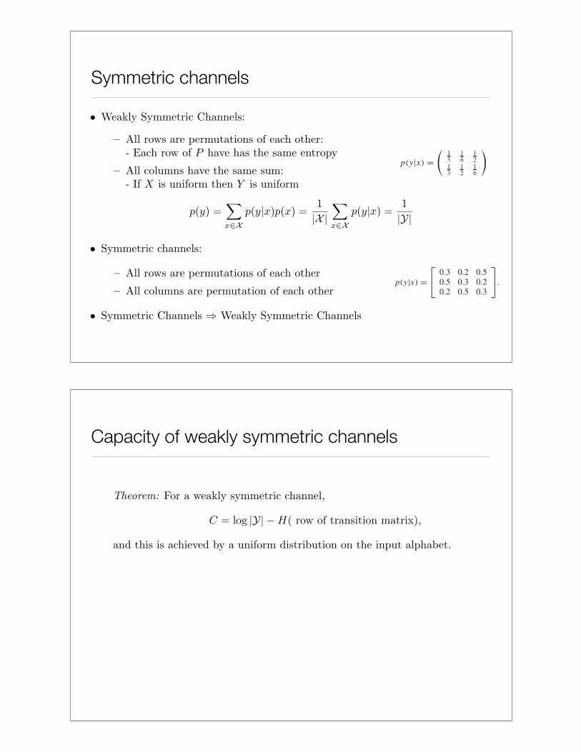
7.2 SYMMETRIC CHANNELS
The capacity of the binary symmetric channel is C = 1 ! H(p) bits pertransmission, and the capacity of the binary erasure channel is C = 1 !! bits per transmission. Now consider the channel with transition matrix:
p(y|x) =
!
"0.3 0.2 0.50.5 0.3 0.20.2 0.5 0.3
#
$. (7.17)
Here the entry in the xth row and the yth column denotes the conditionalprobability p(y|x) that y is received when x is sent. In this channel, allthe rows of the probability transition matrix are permutations of each otherand so are the columns. Such a channel is said to be symmetric. Anotherexample of a symmetric channel is one of the form
Y = X + Z (mod c), (7.18)
190 CHANNEL CAPACITY
where Z has some distribution on the integers {0, 1, 2, . . . , c ! 1}, X hasthe same alphabet as Z, and Z is independent of X.
In both these cases, we can easily find an explicit expression for thecapacity of the channel. Letting r be a row of the transition matrix, wehave
I (X;Y) = H(Y) ! H(Y |X) (7.19)
= H(Y) ! H(r) (7.20)
" log |Y| ! H(r) (7.21)
with equality if the output distribution is uniform. But p(x) = 1/|X|achieves a uniform distribution on Y , as seen from
p(y) =!
x#Xp(y|x)p(x) = 1
|X|!
p(y|x) = c1
|X|= 1
|Y|, (7.22)
where c is the sum of the entries in one column of the probability transitionmatrix.
Thus, the channel in (7.17) has the capacity
C = maxp(x)
I (X;Y) = log 3 ! H(0.5, 0.3, 0.2), (7.23)
and C is achieved by a uniform distribution on the input.The transition matrix of the symmetric channel defined above is doubly
stochastic. In the computation of the capacity, we used the facts that therows were permutations of one another and that all the column sums wereequal.
Considering these properties, we can define a generalization of theconcept of a symmetric channel as follows:
Definition A channel is said to be symmetric if the rows of the channeltransition matrix p(y|x) are permutations of each other and the columnsare permutations of each other. A channel is said to be weakly symmetricif every row of the transition matrix p(·|x) is a permutation of every otherrow and all the column sums
"x p(y|x) are equal.
For example, the channel with transition matrix
p(y|x) =#
13
16
12
13
12
16
$
(7.24)
is weakly symmetric but not symmetric.
Capacity of weakly symmetric channels

Properties of the channel capacityPe =
n!
i=m+1
"n
i
#f i (1! f)n!i
C = maxp(x)
I(X; Y )
C =1
2log2(1 + |h|2P/PN)
C =
$%
&
12 log2(1 + |h|2P/PN)
Eh
'12 log2(1 + |h|2P/PN)
(
C =
$%
&
maxQ:Tr(Q)=P12 log2
))IMR + HQH†))
maxQ:Tr(Q)=P EH
'12 log2
))IMR + HQH†))(
Y = HX + N
X = H!1U + N
"Y = H(H!1U) + N
= U + N
C =1
2log2(1 + P/N)
R2 # I(Y2; X2|X1)
Let Z = (Y1, Y2,X1,X2,V1,V2, W ) be distributed as:
P (w)$ P (m1!|w)P (m1"|w)P (x1|m1!, m1", w)
$ P (m"1!|m1!, w)P (m"
1"|m1", w)P (m2!|v1, w)P (m2"|v1, w)
$ P (x2|m2!, m2",m", w)P (y1|x1,x2)P (y2|x1,x2)
1
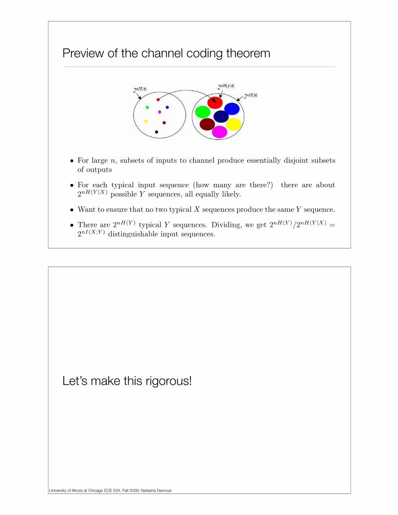
Preview of the channel coding theorem
• What happens when we use the channel n times?
Preview of the channel coding theorem
Review Examples of Channel Channel Capacity Jointly Typical Sequences
Previous of the channel coding theorem
An average input sequence corresponds to about 2nH(Y |X ) typical outputsequences
There are a total of 2nH(Y ) typical output sequences
For nearly error free transmission, we select a number of input sequenceswhose corresponding sets of output sequences hardly overlap
The maximum number of distinct sets of output sequences is2n(H(Y )!H(Y |X )) = 2nI (Y ;X )
B. Smida (ES250) Channel Capacity Fall 2008-09 18 / 22
University of Illinois at Chicago ECE 534, Fall 2009, Natasha Devroye
Let’s make this rigorous!
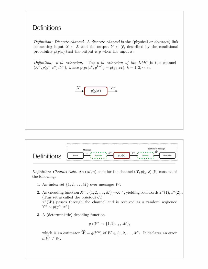
Definitions
Channel
Definitions Source Encoder Channel Decoder Destination
MessageEstimate of message
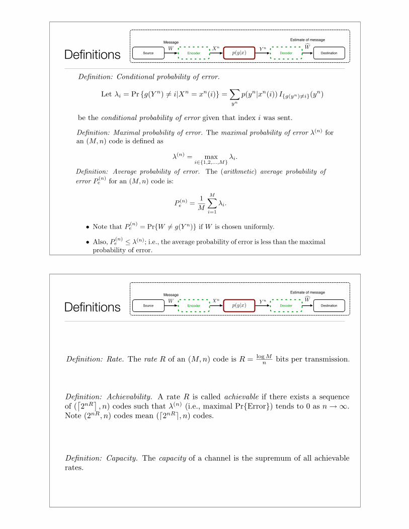
Definitions Source Encoder Channel Decoder Destination
MessageEstimate of message
Definitions Source Encoder Channel Decoder Destination
MessageEstimate of message

University of Illinois at Chicago ECE 534, Fall 2009, Natasha Devroye
What’s our goal?
Mathematical description of capacity
• Information channel capacity:
• Channel coding theorem says: information capacity = operational capacity
Pe =n!
i=m+1
"n
i
#f i (1! f)n!i
C = maxp(x)
I(X; Y )
C =1
2log2(1 + |h|2P/PN)
C =
$%
&
12 log2(1 + |h|2P/PN)
Eh
'12 log2(1 + |h|2P/PN)
(
C =
$%
&
maxQ:Tr(Q)=P12 log2
))IMR + HQH†))
maxQ:Tr(Q)=P EH
'12 log2
))IMR + HQH†))(
Y = HX + N
X = H!1U + N
"Y = H(H!1U) + N
= U + N
C =1
2log2(1 + P/N)
R2 # I(Y2; X2|X1)
Let Z = (Y1, Y2,X1,X2,V1,V2, W ) be distributed as:
P (w)$ P (m1!|w)P (m1"|w)P (x1|m1!, m1", w)
$ P (m"1!|m1!, w)P (m"
1"|m1", w)P (m2!|v1, w)P (m2"|v1, w)
$ P (x2|m2!, m2",m", w)P (y1|x1,x2)P (y2|x1,x2)
1
• Operational channel capacity:
Highest rate (bits/channel use) that can
communicate at reliably
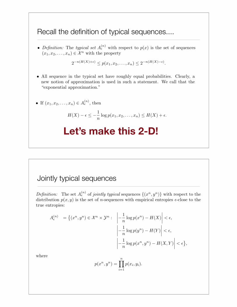
Recall the definition of typical sequences....
Let’s make this 2-D!
Jointly typical sequences
Joint Asymptotic Equipartition Theorem (AEP)
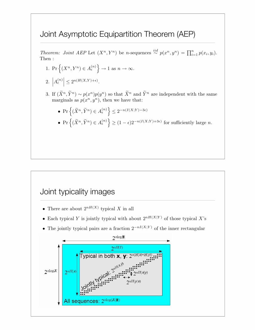
Joint typicality imagesReview Channel Coding Theorem Proof of Achievability Proof of Converse
Jointly Typical Diagram
There are about 2nH(X ) typical X in all
Each typical Y is jointly typical with about 2nH(X |Y ) of those typical X ’s
The jointly typical pairs are a fraction 2!nI (X ;Y ) of the inner rectangular
B. Smida (ES250) Channel Capacity Fall 2008-09 9 / 23
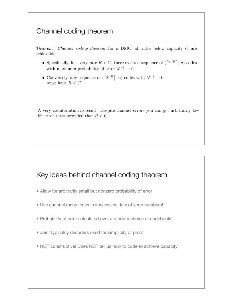
Channel coding theorem
Key ideas behind channel coding theorem
• Allow for arbitrarily small but nonzero probability of error
• Use channel many times in succession: law of large numbers!
• Probability of error calculated over a random choice of codebooks
• Joint typicality decoders used for simplicity of proof
• NOT constructive! Does NOT tell us how to code to achieve capacity!
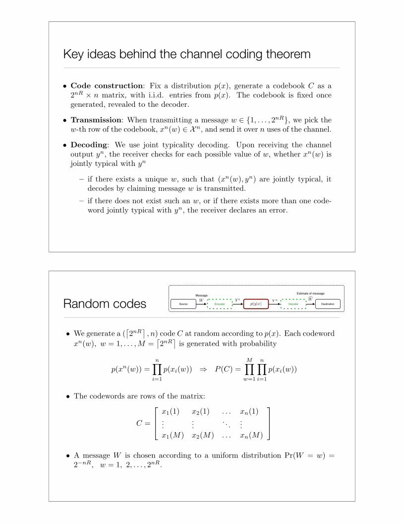
Key ideas behind the channel coding theorem
Random codes Source Encoder Channel Decoder Destination
MessageEstimate of message

Transmission Source Encoder Channel Decoder Destination
MessageEstimate of message
Probability of error Source Encoder Channel Decoder Destination
MessageEstimate of message

Probability of error Source Encoder Channel Decoder Destination
MessageEstimate of message
Random codes? Source Encoder Channel Decoder Destination
MessageEstimate of message

Analogy....
Copyright Cambridge University Press 2003. On-screen viewing permitted. Printing not permitted. http://www.cambridge.org/0521642981
You can buy this book for 30 pounds or $50. See http://www.inference.phy.cam.ac.uk/mackay/itila/ for links.
164 10 — The Noisy-Channel Coding Theorem
! "
#
$ "!2NH(X)
$
#
2NH(Y )
"!
"!2NH(X|Y )
$
#
$
#2NH(Y |X)
! ! ! ! ! ! ! ! ! ! ! ! ! ! ! ! ! ! ! ! !
! ! ! ! ! ! ! ! ! ! ! ! ! ! ! ! ! ! ! ! !
! ! ! ! ! ! ! ! ! ! ! ! ! ! ! ! ! ! ! ! ! !
! ! ! ! ! ! ! ! ! ! ! ! ! ! ! ! ! ! ! ! ! !
! ! ! ! ! ! ! ! ! ! ! ! ! ! ! ! ! ! ! ! !
! ! ! ! ! ! ! ! ! ! ! ! ! ! ! ! ! ! ! ! !
2NH(X,Y ) dots
ANX
ANY
Figure 10.2. The jointly-typicalset. The horizontal directionrepresents AN
X , the set of all inputstrings of length N . The verticaldirection represents AN
Y , the set ofall output strings of length N .The outer box contains allconceivable input–output pairs.Each dot represents ajointly-typical pair of sequences(x,y). The total number ofjointly-typical sequences is about2NH(X,Y ).
10.3 Proof of the noisy-channel coding theorem
Analogy
Imagine that we wish to prove that there is a baby in a class of one hundredbabies who weighs less than 10 kg. Individual babies are di!cult to catch andweigh. Shannon’s method of solving the task is to scoop up all the babies
Figure 10.3. Shannon’s method forproving one baby weighs less than10 kg.
and weigh them all at once on a big weighing machine. If we find that theiraverage weight is smaller than 10 kg, there must exist at least one baby whoweighs less than 10 kg – indeed there must be many! Shannon’s method isn’tguaranteed to reveal the existence of an underweight child, since it relies onthere being a tiny number of elephants in the class. But if we use his methodand get a total weight smaller than 1000 kg then our task is solved.
From skinny children to fantastic codes
We wish to show that there exists a code and a decoder having small prob-ability of error. Evaluating the probability of error of any particular codingand decoding system is not easy. Shannon’s innovation was this: instead ofconstructing a good coding and decoding system and evaluating its error prob-ability, Shannon calculated the average probability of block error of all codes,and proved that this average is small. There must then exist individual codesthat have small probability of block error.
Random coding and typical-set decoding
Consider the following encoding–decoding system, whose rate is R !.
1. We fix P (x) and generate the S = 2NR! codewords of a (N,NR!) =
[Mackay textbook, pg. 164]
Channel coding theorem
Converse to the channel coding theorem
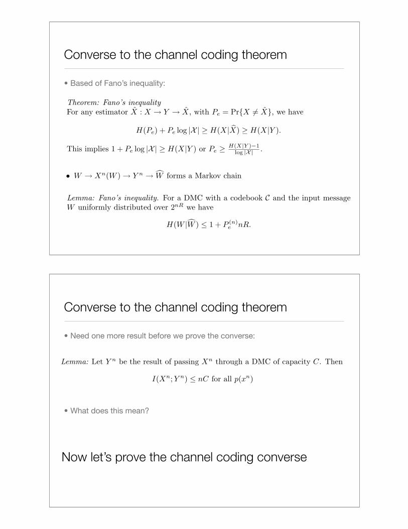
• Based of Fano’s inequality:
Converse to the channel coding theorem
• Need one more result before we prove the converse:
• What does this mean?
Now let’s prove the channel coding converse
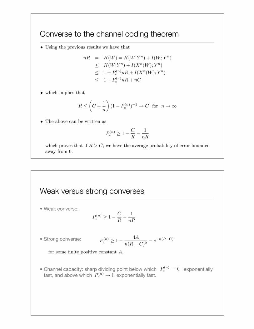
Converse to the channel coding theorem
Weak versus strong converses
• Weak converse:
• Strong converse:
• Channel capacity: sharp dividing point below which exponentially fast, and above which exponentially fast.
Practical coding schemes
SourceSource
coderChannel
Source
decoderDestination
Noise
Channel
coder
Channel
decoder
Encoder Decoder
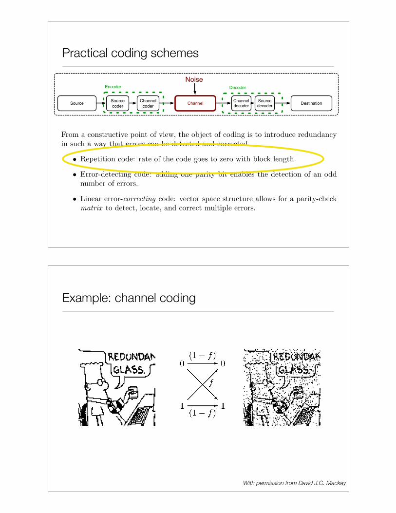
Example: channel coding
With permission from David J.C. Mackay

Example: channel coding
With permission from David J.C. Mackay
Rate?
R = # source bits / # coded bits
Example: channel coding
With permission from David J.C. Mackay
Use repetition code of rate R=1/n: 0 ! 000...0 1 ! 111...1
Decoder? Majority vote
[n=2m+1]Probability of error?
Pe =n!
i=m+1
"n
i
#f i (1! f)n!i
C = maxp(x)
I(X; Y )
C =1
2log2(1 + |h|2P/PN)
C =
$%
&
12 log2(1 + |h|2P/PN)
Eh
'12 log2(1 + |h|2P/PN)
(
C =
$%
&
maxQ:Tr(Q)=P12 log2
))IMR + HQH†))
maxQ:Tr(Q)=P EH
'12 log2
))IMR + HQH†))(
Y = HX + N
X = H!1U + N
"Y = H(H!1U) + N
= U + N
C =1
2log2(1 + P/N)
R2 # I(Y2; X2|X1)
Let Z = (Y1, Y2,X1,X2,V1,V2, W ) be distributed as:
P (w)$ P (m1!|w)P (m1"|w)P (x1|m1!, m1", w)
$ P (m"1!|m1!, w)P (m"
1"|m1", w)P (m2!|v1, w)P (m2"|v1, w)
$ P (x2|m2!, m2",m", w)P (y1|x1,x2)P (y2|x1,x2)
1
Need n !! for reliable communication!
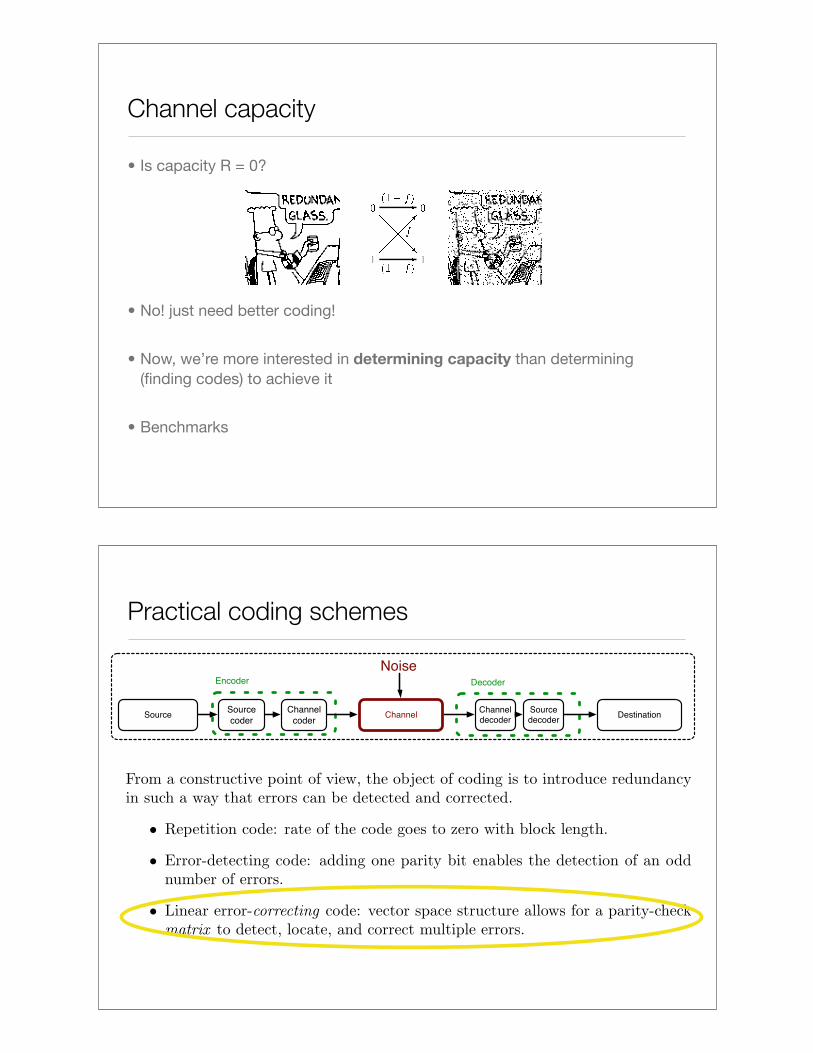
Channel capacity
• Is capacity R = 0?
• No! just need better coding!
• Now, we’re more interested in determining capacity than determining
(finding codes) to achieve it
• Benchmarks
Practical coding schemes
SourceSource
coderChannel
Source
decoderDestination
Noise
Channel
coder
Channel
decoder
Encoder Decoder

Linear block codes
Properties of linear block codes

Properties of linear block codes
Examples
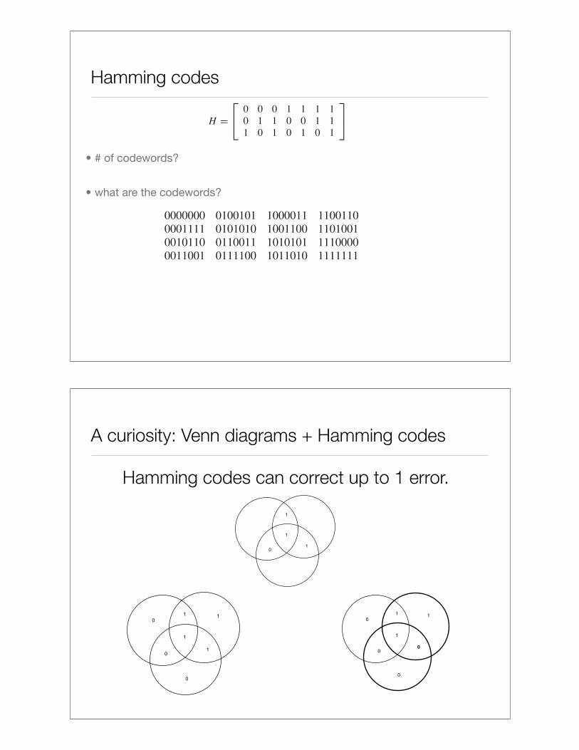
Hamming codes
• # of codewords?
• what are the codewords?
7.11 HAMMING CODES 211
the block as a 1; otherwise, we decode it as 0. An error occurs if andonly if more than three of the bits are changed. By using longer repetitioncodes, we can achieve an arbitrarily low probability of error. But the rateof the code also goes to zero with block length, so even though the codeis “simple,” it is really not a very useful code.
Instead of simply repeating the bits, we can combine the bits in someintelligent fashion so that each extra bit checks whether there is an error insome subset of the information bits. A simple example of this is a paritycheck code. Starting with a block of n ! 1 information bits, we choosethe nth bit so that the parity of the entire block is 0 (the number of 1’sin the block is even). Then if there is an odd number of errors duringthe transmission, the receiver will notice that the parity has changed anddetect the error. This is the simplest example of an error-detecting code.The code does not detect an even number of errors and does not give anyinformation about how to correct the errors that occur.
We can extend the idea of parity checks to allow for more than oneparity check bit and to allow the parity checks to depend on various subsetsof the information bits. The Hamming code that we describe below is anexample of a parity check code. We describe it using some simple ideasfrom linear algebra.
To illustrate the principles of Hamming codes, we consider a binarycode of block length 7. All operations will be done modulo 2. Considerthe set of all nonzero binary vectors of length 3. Arrange them in columnsto form a matrix:
H =
!
"0 0 0 1 1 1 10 1 1 0 0 1 11 0 1 0 1 0 1
#
$. (7.117)
Consider the set of vectors of length 7 in the null space of H (the vectorswhich when multiplied by H give 000). From the theory of linear spaces,since H has rank 3, we expect the null space of H to have dimension 4.These 24 codewords are
0000000 0100101 1000011 11001100001111 0101010 1001100 11010010010110 0110011 1010101 11100000011001 0111100 1011010 1111111
Since the set of codewords is the null space of a matrix, it is linear in thesense that the sum of any two codewords is also a codeword. The set ofcodewords therefore forms a linear subspace of dimension 4 in the vectorspace of dimension 7.
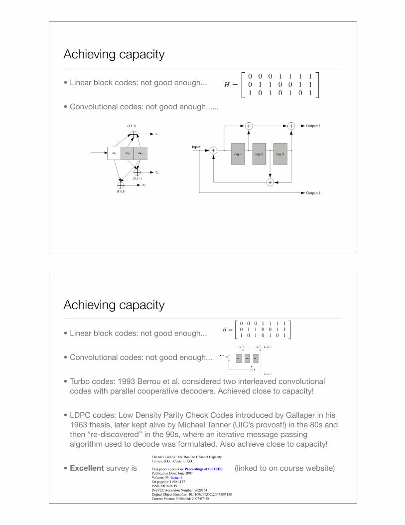
A curiosity: Venn diagrams + Hamming codes
7.11 HAMMING CODES 213
codeword represent the message, and the last n ! k bits are parity checkbits. Such a code is called a systematic code. The code is often identifiedby its block length n, the number of information bits k and the minimumdistance d. For example, the above code is called a (7,4,3) Hamming code(i.e., n = 7, k = 4, and d = 3).
An easy way to see how Hamming codes work is by means of a Venndiagram. Consider the following Venn diagram with three circles and withfour intersection regions as shown in Figure 7.10. To send the informationsequence 1101, we place the 4 information bits in the four intersectionregions as shown in the figure. We then place a parity bit in each of thethree remaining regions so that the parity of each circle is even (i.e., thereare an even number of 1’s in each circle). Thus, the parity bits are asshown in Figure 7.11.
Now assume that one of the bits is changed; for example one of theinformation bits is changed from 1 to 0 as shown in Figure 7.12. Thenthe parity constraints are violated for two of the circles (highlighted in thefigure), and it is not hard to see that given these violations, the only singlebit error that could have caused it is at the intersection of the two circles(i.e., the bit that was changed). Similarly working through the other errorcases, it is not hard to see that this code can detect and correct any singlebit error in the received codeword.
We can easily generalize this procedure to construct larger matricesH . In general, if we use l rows in H , the code that we obtain will haveblock length n = 2l ! 1, k = 2l ! l ! 1 and minimum distance 3. Allthese codes are called Hamming codes and can correct one error.
1
1
01
FIGURE 7.10. Venn diagram with information bits.
Hamming codes can correct up to 1 error.
214 CHANNEL CAPACITY
0
1
1
01
01
FIGURE 7.11. Venn diagram with information bits and parity bits with even parity for eachcircle.
0
1
1
0
01
0
FIGURE 7.12. Venn diagram with one of the information bits changed.
Hamming codes are the simplest examples of linear parity check codes.They demonstrate the principle that underlies the construction of otherlinear codes. But with large block lengths it is likely that there will bemore than one error in the block. In the early 1950s, Reed and Solomonfound a class of multiple error-correcting codes for nonbinary channels.In the late 1950s, Bose and Ray-Chaudhuri [72] and Hocquenghem [278]generalized the ideas of Hamming codes using Galois field theory to con-struct t-error correcting codes (called BCH codes) for any t . Since then,various authors have developed other codes and also developed efficient
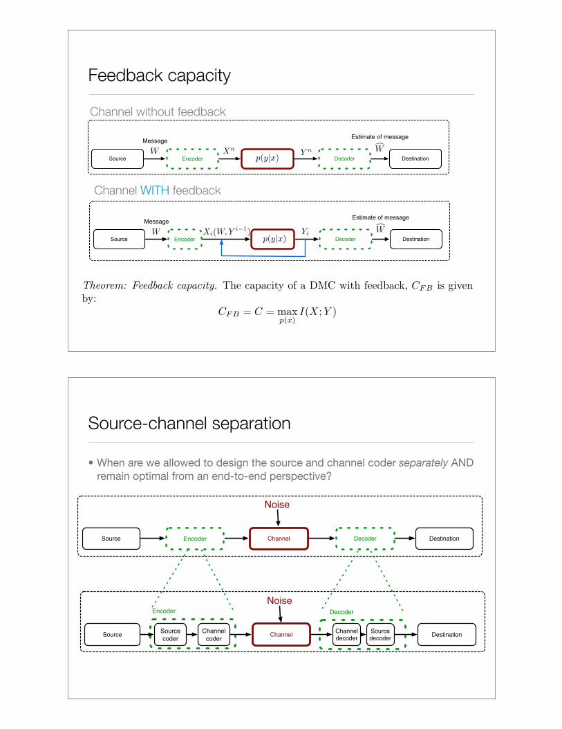
Achieving capacity
• Linear block codes: not good enough...
• Convolutional codes: not good enough......
7.11 HAMMING CODES 211
the block as a 1; otherwise, we decode it as 0. An error occurs if andonly if more than three of the bits are changed. By using longer repetitioncodes, we can achieve an arbitrarily low probability of error. But the rateof the code also goes to zero with block length, so even though the codeis “simple,” it is really not a very useful code.
Instead of simply repeating the bits, we can combine the bits in someintelligent fashion so that each extra bit checks whether there is an error insome subset of the information bits. A simple example of this is a paritycheck code. Starting with a block of n ! 1 information bits, we choosethe nth bit so that the parity of the entire block is 0 (the number of 1’sin the block is even). Then if there is an odd number of errors duringthe transmission, the receiver will notice that the parity has changed anddetect the error. This is the simplest example of an error-detecting code.The code does not detect an even number of errors and does not give anyinformation about how to correct the errors that occur.
We can extend the idea of parity checks to allow for more than oneparity check bit and to allow the parity checks to depend on various subsetsof the information bits. The Hamming code that we describe below is anexample of a parity check code. We describe it using some simple ideasfrom linear algebra.
To illustrate the principles of Hamming codes, we consider a binarycode of block length 7. All operations will be done modulo 2. Considerthe set of all nonzero binary vectors of length 3. Arrange them in columnsto form a matrix:
H =
!
"0 0 0 1 1 1 10 1 1 0 0 1 11 0 1 0 1 0 1
#
$. (7.117)
Consider the set of vectors of length 7 in the null space of H (the vectorswhich when multiplied by H give 000). From the theory of linear spaces,since H has rank 3, we expect the null space of H to have dimension 4.These 24 codewords are
0000000 0100101 1000011 11001100001111 0101010 1001100 11010010010110 0110011 1010101 11100000011001 0111100 1011010 1111111
Since the set of codewords is the null space of a matrix, it is linear in thesense that the sum of any two codewords is also a codeword. The set ofcodewords therefore forms a linear subspace of dimension 4 in the vectorspace of dimension 7.
Achieving capacity
• Linear block codes: not good enough...
• Convolutional codes: not good enough...
• Turbo codes: 1993 Berrou et al. considered two interleaved convolutional codes with parallel cooperative decoders. Achieved close to capacity!
• LDPC codes: Low Density Parity Check Codes introduced by Gallager in his 1963 thesis, later kept alive by Michael Tanner (UIC’s provost!) in the 80s and then “re-discovered” in the 90s, where an iterative message passing algorithm used to decode was formulated. Also achieve close to capacity!
• Excellent survey is (linked to on course website)
7.11 HAMMING CODES 211
the block as a 1; otherwise, we decode it as 0. An error occurs if andonly if more than three of the bits are changed. By using longer repetitioncodes, we can achieve an arbitrarily low probability of error. But the rateof the code also goes to zero with block length, so even though the codeis “simple,” it is really not a very useful code.
Instead of simply repeating the bits, we can combine the bits in someintelligent fashion so that each extra bit checks whether there is an error insome subset of the information bits. A simple example of this is a paritycheck code. Starting with a block of n ! 1 information bits, we choosethe nth bit so that the parity of the entire block is 0 (the number of 1’sin the block is even). Then if there is an odd number of errors duringthe transmission, the receiver will notice that the parity has changed anddetect the error. This is the simplest example of an error-detecting code.The code does not detect an even number of errors and does not give anyinformation about how to correct the errors that occur.
We can extend the idea of parity checks to allow for more than oneparity check bit and to allow the parity checks to depend on various subsetsof the information bits. The Hamming code that we describe below is anexample of a parity check code. We describe it using some simple ideasfrom linear algebra.
To illustrate the principles of Hamming codes, we consider a binarycode of block length 7. All operations will be done modulo 2. Considerthe set of all nonzero binary vectors of length 3. Arrange them in columnsto form a matrix:
H =
!
"0 0 0 1 1 1 10 1 1 0 0 1 11 0 1 0 1 0 1
#
$. (7.117)
Consider the set of vectors of length 7 in the null space of H (the vectorswhich when multiplied by H give 000). From the theory of linear spaces,since H has rank 3, we expect the null space of H to have dimension 4.These 24 codewords are
0000000 0100101 1000011 11001100001111 0101010 1001100 11010010010110 0110011 1010101 11100000011001 0111100 1011010 1111111
Since the set of codewords is the null space of a matrix, it is linear in thesense that the sum of any two codewords is also a codeword. The set ofcodewords therefore forms a linear subspace of dimension 4 in the vectorspace of dimension 7.
Channel Coding: The Road to Channel Capacity
Forney, G.D.!! Costello, D.J.!!
This paper appears in: Proceedings of the IEEE
Publication Date: June 2007
Volume: 95,! Issue: 6
On page(s): 1150-1177
ISSN: 0018-9219
INSPEC Accession Number: 9629854
Digital Object Identifier: 10.1109/JPROC.2007.895188
Current Version Published: 2007-07-30

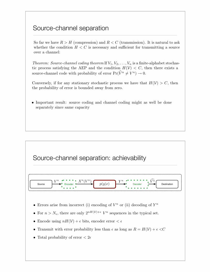
Feedback capacity
Source Encoder Channel Decoder Destination
MessageEstimate of message
Channel without feedback
Channel WITH feedback
Source Encoder Decoder Destination
MessageEstimate of message
Feedback capacity
Feedback capacity
Source Encoder Channel Decoder Destination
MessageEstimate of message
Channel without feedback
Channel WITH feedback
Source Encoder Decoder Destination
MessageEstimate of message
Source-channel separation
• When are we allowed to design the source and channel coder separately AND remain optimal from an end-to-end perspective?
Source Encoder Channel Decoder Destination
Noise
SourceSource
coderChannel
Source
decoderDestination
Noise
Channel
coder
Channel
decoder
Encoder Decoder
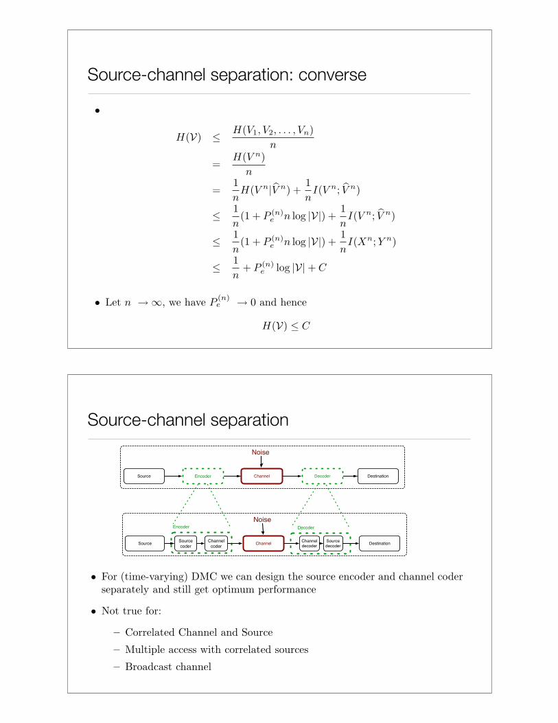
Source-channel separation
Source-channel separation: achievability
Source Encoder Channel Decoder Destination
Source-channel separation: converse
Source-channel separation
Source Encoder Channel Decoder Destination
Noise
SourceSource
coderChannel
Source
decoderDestination
Noise
Channel
coder
Channel
decoder
Encoder Decoder