comp of clustering method
TRANSCRIPT
8/8/2019 Comp of Clustering Method
http://slidepdf.com/reader/full/comp-of-clustering-method 1/117
8/8/2019 Comp of Clustering Method
http://slidepdf.com/reader/full/comp-of-clustering-method 2/117
Contents
0.1 Preface . . . . . . . . . . . . . . . . . . . . . . . . . . . . . . . 1
1 Introduction 21.1 Motivation . . . . . . . . . . . . . . . . . . . . . . . . . . . . . 21.2 Goal of the thesis . . . . . . . . . . . . . . . . . . . . . . . . . 31.3 Related works . . . . . . . . . . . . . . . . . . . . . . . . . . . 41.4 Thesis organization . . . . . . . . . . . . . . . . . . . . . . . . 4
2 Background 62.1 Introduction to computer network security . . . . . . . . . . . 6
2.1.1 Network security . . . . . . . . . . . . . . . . . . . . . 62.1.2 Network intrusion detection systems . . . . . . . . . . 72.1.3 Network anomaly detection . . . . . . . . . . . . . . . 8
2.1.4 Computer attacks . . . . . . . . . . . . . . . . . . . . . 92.2 Introduction to clustering . . . . . . . . . . . . . . . . . . . . 12
2.2.1 Notation and definitions . . . . . . . . . . . . . . . . . 122.2.2 The clustering problem . . . . . . . . . . . . . . . . . . 122.2.3 The clustering process . . . . . . . . . . . . . . . . . . 132.2.4 Feature selection . . . . . . . . . . . . . . . . . . . . . 132.2.5 Choice of clustering algorithm . . . . . . . . . . . . . . 132.2.6 Cluster validity . . . . . . . . . . . . . . . . . . . . . . 162.2.7 Clustering tendency . . . . . . . . . . . . . . . . . . . . 172.2.8 Clustering of network traffic data . . . . . . . . . . . . 18
2.3 Summary . . . . . . . . . . . . . . . . . . . . . . . . . . . . . 19
3 Clustering methods and algorithms 203.1 Hierarchical clustering methods . . . . . . . . . . . . . . . . . 213.2 Partitioning clustering methods . . . . . . . . . . . . . . . . . 24
3.2.1 Squared-error clustering . . . . . . . . . . . . . . . . . 24
1
8/8/2019 Comp of Clustering Method
http://slidepdf.com/reader/full/comp-of-clustering-method 3/117
CONTENTS 2
3.2.2 Model-based clustering . . . . . . . . . . . . . . . . . . 27
3.2.3 Density-based clustering . . . . . . . . . . . . . . . . . 423.2.4 Grid-based clustering . . . . . . . . . . . . . . . . . . . 453.2.5 Online clustering . . . . . . . . . . . . . . . . . . . . . 473.2.6 Fuzzy clustering . . . . . . . . . . . . . . . . . . . . . . 48
3.3 Discussion of the classical clustering methods . . . . . . . . . 523.4 Combining clustering methods . . . . . . . . . . . . . . . . . . 54
3.4.1 Two-level clustering with kmeans . . . . . . . . . . . . 543.4.2 Initialisation of clustering algorithms with the results
of leader clustering . . . . . . . . . . . . . . . . . . . . 603.5 Summary . . . . . . . . . . . . . . . . . . . . . . . . . . . . . 61
4 Experiments 624.1 Design of the experiments . . . . . . . . . . . . . . . . . . . . 624.2 Data set . . . . . . . . . . . . . . . . . . . . . . . . . . . . . . 63
4.2.1 Choice of data set . . . . . . . . . . . . . . . . . . . . . 634.2.2 Description of the feature set . . . . . . . . . . . . . . 65
4.3 Implementation issues . . . . . . . . . . . . . . . . . . . . . . 694.4 Summary . . . . . . . . . . . . . . . . . . . . . . . . . . . . . 71
5 Evaluation of clustering methods 725.1 Evaluation methodology . . . . . . . . . . . . . . . . . . . . . 72
5.2 Evaluation measures . . . . . . . . . . . . . . . . . . . . . . . 735.2.1 Evaluation measure requirements . . . . . . . . . . . . 745.2.2 Choice of evaluation measures . . . . . . . . . . . . . . 74
5.3 k-fold cross validation . . . . . . . . . . . . . . . . . . . . . . . 765.4 Discussion and analysis of the experiment results . . . . . . . 76
5.4.1 Results of the experiments . . . . . . . . . . . . . . . . 765.4.2 Analysis of the experiment results . . . . . . . . . . . . 79
6 Conclusion 866.1 Resume . . . . . . . . . . . . . . . . . . . . . . . . . . . . . . 86
6.2 Achievements . . . . . . . . . . . . . . . . . . . . . . . . . . . 876.3 Limitations . . . . . . . . . . . . . . . . . . . . . . . . . . . . 886.4 Future work . . . . . . . . . . . . . . . . . . . . . . . . . . . . 89
8/8/2019 Comp of Clustering Method
http://slidepdf.com/reader/full/comp-of-clustering-method 4/117
CONTENTS 3
A Definitions 95
A.1 Acronyms . . . . . . . . . . . . . . . . . . . . . . . . . . . . . 95A.2 Definitions . . . . . . . . . . . . . . . . . . . . . . . . . . . . 95
B Feature set 98B.1 The feature set of the KDD Cup 99 data set . . . . . . . . . . 98
C Computer attacks 101C.1 Probe attacks . . . . . . . . . . . . . . . . . . . . . . . . . . . 101C.2 Denial of service attacks . . . . . . . . . . . . . . . . . . . . . 102C.3 User to root attacks . . . . . . . . . . . . . . . . . . . . . . . . 102C.4 Remote to local attacks . . . . . . . . . . . . . . . . . . . . . . 103C.5 Other attack scenarios . . . . . . . . . . . . . . . . . . . . . . 104
D Theorems 105D.1 Algorithm: Hill climbing . . . . . . . . . . . . . . . . . . . . . 105D.2 Theorem: Jensen’s inequality . . . . . . . . . . . . . . . . . . 105D.3 Theorem: The Lagrange method . . . . . . . . . . . . . . . . 106
E Results of the experiments 107
8/8/2019 Comp of Clustering Method
http://slidepdf.com/reader/full/comp-of-clustering-method 5/117
List of Figures
3.1 A dendrogram corresponding to the distance matrix in table 3.1 22
3.2 Variation of the sum of squared-errors in kmeans . . . . . . . 283.3 Variation of the log-likelihood with the iterations of the clas-sification maximum likelihood . . . . . . . . . . . . . . . . . . 38
3.4 A 3x3 kohonen network map . . . . . . . . . . . . . . . . . . . 403.5 Querying recursively a multi-resolution grid with STING . . . 453.6 Variation of the - fuzzy - sum of squared errors in fuzzy kmeans
algorithm . . . . . . . . . . . . . . . . . . . . . . . . . . . . . 523.7 Variation of classification accuracy with the number of basic
clusters . . . . . . . . . . . . . . . . . . . . . . . . . . . . . . . 583.8 Variation of the sum of squared-errors(SSE) with the number
of clusters in kmeans . . . . . . . . . . . . . . . . . . . . . . . 59
5.1 The classification accuracy of the clustering algorithms in ta-bles E.1 and E.2. L+kmeans refers to leader + kmeans andfuzzy K refers to fuzzy kmeans. The number of clusters is 23. 77
5.2 The number of different cluster categories found by the algo-rithms when the number of clusters is 23. The total numberof labels contained in the data set is 23. . . . . . . . . . . . . 81
5.3 The cluster entropies when the number of clusters is 23. Thecluster entropy measures the homogeneity of the clusters. Thelower the cluster entropy is the more homogeneous the clusters
are. . . . . . . . . . . . . . . . . . . . . . . . . . . . . . . . . . 825.4 The classification accuracy of the clustering algorithms in ta-
bles E.3 and E.4. The number of clusters is 49. . . . . . . . . 835.5 The number of different cluster categories found by the algo-
rithms when the number of clusters is 49. The total numberof labels contained in the data set is 23. . . . . . . . . . . . . 84
4

8/8/2019 Comp of Clustering Method
http://slidepdf.com/reader/full/comp-of-clustering-method 6/117
LIST OF FIGURES 5
5.6 The cluster entropies when the number of clusters is 49. . . . . 85
8/8/2019 Comp of Clustering Method
http://slidepdf.com/reader/full/comp-of-clustering-method 7/117
List of Tables
3.1 Example of distance matrix used for hierarchical clustering . . 21
4.1 Distribution of labels in the data set . . . . . . . . . . . . . . 70
B.1 Basic features of the KDD Cup 99 data set . . . . . . . . . . . 99B.2 Content-based features . . . . . . . . . . . . . . . . . . . . . . 99B.3 Traffic-based features . . . . . . . . . . . . . . . . . . . . . . . 100
E.1 Random initialisation . . . . . . . . . . . . . . . . . . . . . . . 108E.2 Experimental results of various classical algorithms and com-
bination of those algorithms run on a KDD Cup 1999 data setslightly modified. The number of clusters is set to the numberof attack and normal labels in the data set and this numberis 23. The results in table E.1 are obtained with random ini-tialisation of the algorithms and that of table E.2 correspondto initialisation of the algorithms with leader clustering. . . . 108
E.3 Random initialisation . . . . . . . . . . . . . . . . . . . . . . . 108E.4 Experiment results when the number of clusters is 49 . . . . . 109
6
8/8/2019 Comp of Clustering Method
http://slidepdf.com/reader/full/comp-of-clustering-method 8/117
8/8/2019 Comp of Clustering Method
http://slidepdf.com/reader/full/comp-of-clustering-method 9/117
LIST OF TABLES 2
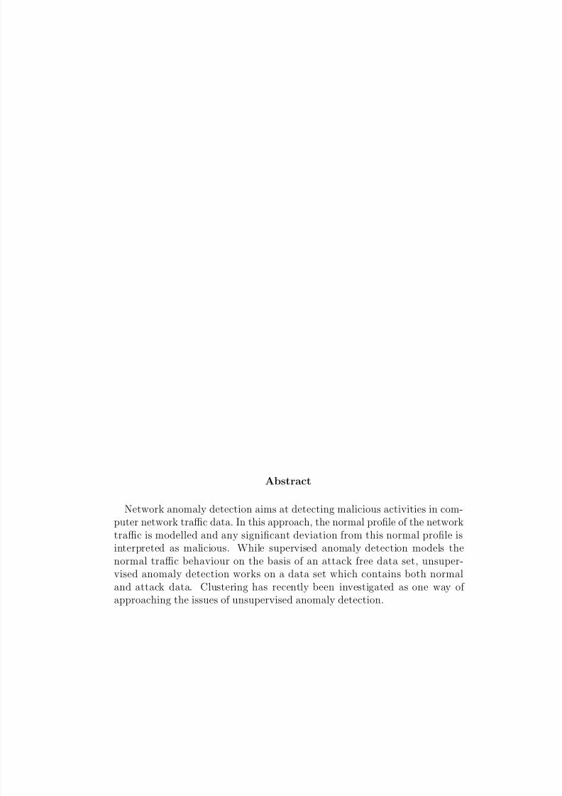
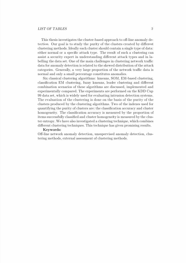
This thesis investigates the cluster-based approach to off-line anomaly de-
tection. Our goal is to study the purity of the clusters created by differentclustering methods. Ideally each cluster should contain a single type of data:either normal or a specific attack type. The result of such a clustering canassist a security expert in understanding different attack types and in la-belling the data set. One of the main challenges in clustering network trafficdata for anomaly detection is related to the skewed distribution of the attackcategories. Generally, a very large proportion of the network traffic data isnormal and only a small percentage constitutes anomalies.
Six classical clustering algorithms: kmeans, SOM, EM-based clustering,classification EM clustering, fuzzy kmeans, leader clustering and different
combination scenarios of these algorithms are discussed, implemented andexperimentally compared. The experiments are performed on the KDD Cup99 data set, which is widely used for evaluating intrusion detection systems.The evaluation of the clustering is done on the basis of the purity of theclusters produced by the clustering algorithms. Two of the indexes used forquantifying the purity of clusters are: the classification accuracy and clusterhomogeneity. The classification accuracy is measured by the proportion of items successfully classified and cluster homogeneity is measured by the clus-ter entropy. We have also investigated a clustering technique, which combinesdifferent clustering techniques. This technique has given promising results.
Keywords:Off-line network anomaly detection, unsupervised anomaly detection, clus-tering methods, external assessment of clustering methods.

8/8/2019 Comp of Clustering Method
http://slidepdf.com/reader/full/comp-of-clustering-method 10/117
LIST OF TABLES 1
0.1 Preface
This thesis has been written by koffi bruno yao at the department of computerscience of the university of copenhagen(DIKU). The thesis was written inthe period 19/04/2005 to 01/03/2006 and was supervised by Peter Johansenprofessor at DIKU. I would like to thank my supervisor for his support. Theprimary audience of this thesis is researchers in anomaly detection. Howeverany reader with interest in clustering will find the thesis useful. The reader isexpected to have some basic understandings of computer networks and somebasic mathematical knowledge.
8/8/2019 Comp of Clustering Method
http://slidepdf.com/reader/full/comp-of-clustering-method 11/117
Chapter 1
Introduction
1.1 Motivation
It is important for companies to keep their computer systems secure be-cause their economical activities rely on it. Despite the existence of attackprevention mechanisms such as firewalls, most company computer networksare still the victim of attacks. According to the statistics of CERT [44], thenumber of reported incidents against computer networks has increased from252 in 1990 to 21756 in 2000, and to 137529 in 2003. This happened becauseof misconfiguration of firewalls or because malicious activities are generallycleverly designed to circumvent the firewall policies. It is therefore crucial tohave another line of defence in order to detect and stop malicious activities.This line of defence is intrusion detection systems (IDS).
During the last decades, different approaches to intrusion detection havebeen explored. The two most common approaches are misuse detection andanomaly detection. In misuse detection, attacks are detected by matchingthe current traffic pattern with the signature of known attacks. Anomalydetection keeps a profile of normal system behaviour and interprets any sig-nificant deviation from this normal profile as malicious activity. One of thestrengths of anomaly detection is the ability to detect new attacks. Anomalydetection’s most serious weakness is that it generates too many false alarms.Anomaly detection falls into two categories: supervised anomaly detectionand unsupervised anomaly detection. In supervised anomaly detection, theinstances of the data set used for training the system are labelled either as
2
8/8/2019 Comp of Clustering Method
http://slidepdf.com/reader/full/comp-of-clustering-method 12/117
CHAPTER 1. INTRODUCTION 3
normal or as specific attack type. The problem with this approach is that la-
belling the data is time consuming. Unsupervised anomaly detection, on theother hand, operates on unlabeled data. The advantage of using unlabeleddata is that the unlabeled data is easy and inexpensive to obtain. The mainchallenge in performing unsupervised anomaly detection is distinguishing thenormal data patterns from attack data patterns.
Recently, clustering has been investigated as one approach to solving thisproblem. As attack data patterns are assumed to differ from normal datapatterns, clustering can be used to distinguish attack data patterns fromnormal data patterns. Clustering network traffic data is difficult because:
1. of high data volume
2. of high data dimension
3. the distribution of attack and normal classes is skewed
4. the data is a mixture of categorical and continuous data
5. of the pre-processing of the data required.
1.2 Goal of the thesisAlthough different clustering algorithms have been studied for this pur-
pose, to our knowledge not much has been done in the direction of comparingand combining different clustering approaches. We believe that such a studycould help in designing the most appropriate clustering approaches for thepurpose of unsupervised anomaly detection.The main goals of this thesis are:
1. to provide a comprehensive study of the clustering problem and thedifferent methods used to solve it
2. to implement and compare experimentally some classical clustering al-gorithms
3. and to combine different clustering approaches.

8/8/2019 Comp of Clustering Method
http://slidepdf.com/reader/full/comp-of-clustering-method 13/117
CHAPTER 1. INTRODUCTION 4
1.3 Related works
Clustering has been studied in many scientific disciplines. A wide varietyof algorithms are found in clustering literature. [2] gives a good review of themain classical clustering concepts and algorithms. [3, 20] provide an excellentmathematical approach to the clustering problem. [23] is also an excellentsource; it covers all the main steps in clustering. It discusses clusteringfrom a statistical perspective. [10, 18] present recently developed clusteringalgorithms for clustering large data sets.
There are in the literature many examples of experimental comparisons of
clustering algorithms. Some examples of recent works are found in [35, 12]. In[35], dynamical clustering, kmeans, SOM, hierarchical agglomerative cluster-ing and CLICK have been compared for gene expression data. [12] compareskmeans, SOM and ART-C on text documents. These comparisons differ asto the selection of clustering algorithms, the data set, and the evaluation cri-teria used for assessing the algorithms or the evaluation methodology. Someof these experiments compare clusters on the basis of internal criteria such asthe number of clusters, compactness and separability of clusters, while otherworks compare clustering algorithms on the basis of external indices. Anexternal index measures how well a partition created by a given clusteringalgorithm matches an a priori partitioning of the data set. Our choice of clus-tering algorithms, data set, evaluation criterion and evaluation methodologydistinguishes our work from these works.
[9] provides a good review of data mining approaches for intrusion detec-tion. Much work has been done on the area of unsupervised anomaly detec-tion [7, 4, 6]. In [4], Eskin uses clustering to group normal data; intrusionsare considered to be outliers. Eskin follows a probability based approach tooutliers’ detection. In this approach, the data space has an unknown proba-bility distribution. In this data space, anomalies are located in sparse regionswhile normal data are found in dense regions.
1.4 Thesis organization
This thesis is composed of two main parts:

8/8/2019 Comp of Clustering Method
http://slidepdf.com/reader/full/comp-of-clustering-method 14/117
CHAPTER 1. INTRODUCTION 5
•A theoretical part, in which the clustering problem and the different
clustering methods are studied. This part consists in chapter 2 and3. Chapter 2 is an introduction to anomaly detection and clustering.Chapter 3 discusses the different clustering methods. In conclusion,different combinations of these methods are proposed.
• An experimental part which consists in chapters 4 and 5. In chapter 4,the data set, and the design of the experiments are discussed. Chapter5 discusses the evaluation of clustering methods. Chapter 6 concludesthe thesis.
The
8/8/2019 Comp of Clustering Method
http://slidepdf.com/reader/full/comp-of-clustering-method 15/117
Chapter 2
Background
This chapter provides background in network security and clustering relevantfor understanding the thesis.
• Section 2.1 gives an introduction to network security. The definitionsof network terminologies, frequently used in this thesis, are found inappendix A.
• Section 2.2 gives an introduction to clustering.
• Section 2.3 summarizes this chapter.
2.1 Introduction to computer network secu-rity
Computer networks interconnect multiple computers and make it easy andfast to share resources between these computers. The most popular exampleof such a network is the global Internet. In this thesis, the term computernetworks mainly refers to private computer networks, geographically limitedand connected to the outside world. The main threats to computer networksare security issues. This section will give a brief discussion of some of the
main issues pertaining to network security.
2.1.1 Network security
Computer network security aims at preventing, detecting and stopping anyactivity that has the potential of compromising the confidentiality and in-
6
8/8/2019 Comp of Clustering Method
http://slidepdf.com/reader/full/comp-of-clustering-method 16/117
CHAPTER 2. BACKGROUND 7
tegrity of communication on the network as well as the availability of the
network’s resources and services. Another goal of security is to recover fromsuch malicious activities when they take place. Attack prevention is generallyimplemented by security mechanisms such as authentication, cryptographyand firewalls. Although attack prevention mechanisms are crucial, they arenot enough for assuring the security of the network. Firewalls, for example,can prevent malicious activities from penetrating into the internal network,but they are not able to prevent malicious activities that are initiated frominside the network. Firewalls can also be subject to attacks and preventedfrom working by for example denial of service (DOS) attacks. Attacks canalso pass through firewalls successfully because the firewalls have been mis-
configured. Because of these weaknesses in prevention mechanisms, computernetworks will always be vulnerable to malicious activities.Attack detection and recovery mechanisms complement attack prevention
mechanisms. This function of detection and recovery is mainly implementedby intrusion detection systems. A distinction is made between host-basedintrusion detection systems (HIDS) and network based intrusion detectionsystems (NIDS). HIDS detect intrusions directed against a single host. NIDSdetect intrusions directed against the entire network. In this thesis, we willfocus on network intrusion detection. In the next section, we will presentsystems for network intrusion detection. We will discuss their architecture,and the different steps followed when dealing with intrusion.
2.1.2 Network intrusion detection systems
In this thesis, we cluster data for network intrusion detection. This sectiondiscusses how the input data and the clustering result fit into the architectureof network intrusion detection systems. Network intrusion detection systemsare designed to detect the presence of malicious activities on the network.
The architecture of network intrusion detection systems generally consistsof three parts: agent, detector and notifier. Agents gather network trafficdata, detectors analyse the information gathered by agents to determine the
presence of attacks. The notifier makes decision as to whether a notificationabout the presence of an intrusion should be sent. The same software canperform all these task in a simple network. In more complex networks, thesefunctions are distributed over the network for reasons of security, efficiency,scalability and robustness.
In the context of this thesis, only agents and detectors are relevant.
8/8/2019 Comp of Clustering Method
http://slidepdf.com/reader/full/comp-of-clustering-method 17/117
CHAPTER 2. BACKGROUND 8
Agents generally gather network traffic data by sniffing the network. Sniff-
ing the network involves the agent having access to all the network traffic.In an Ethernet-based network one computer can play the role of an agent.Agents generally process the gathered data into a format that is easy for thedetector to use. The detector can use different techniques for the detectionof intrusions. The two main techniques are misuse detection and anomalydetection. Misuse detection detects attacks by matching the current networktraffic against a database of known attack signatures. Anomaly detection,on the other hand, finds attacks by identifying traffic patterns that deviatesignificantly from the normal traffic.
The data set used in this thesis is an example of data obtained from
network intrusion detection agents. The output of the clustering serves todefine or enrich models used by the detector.In the next section, we will look at network anomaly detection, which is
the type of detection technique we are interested in in this thesis.
2.1.3 Network anomaly detection
As we explained earlier, detectors need models or rules for detecting intru-sions. These models can be built off-line on the basis of earlier network trafficdata gathered by agents. Once the model has been built, the task of detect-ing and stopping intrusions can be performed online. One of the weaknessesof this approach is that it is not adaptive. This is because small changes intraffic affect the model globally. Some approaches to anomaly detection per-form the model construction and anomaly detection simultaneously on-line.In some of these approaches clustering has been used. One of the advan-tages of online modelling is that it is less time consuming because it doesnot require a separate training phase. Furthermore, the model reflects thecurrent nature of network traffic. The problem with this approach is that itcan lead to inaccurate models. This happens because this approach fails todetect attacks performed systematically over a long period of time. Thesetypes of attacks can only be detected by analysing network traffic gathered
over a long period of time.The clusters obtained by clustering network traffic data off-line can be
used for either anomaly detection or misuse detection. For anomaly detec-tion, it is the clusters formed by the normal data that are relevant for modelconstruction. For misuse detection, it is the different attack clusters that areused for model construction.
8/8/2019 Comp of Clustering Method
http://slidepdf.com/reader/full/comp-of-clustering-method 18/117
CHAPTER 2. BACKGROUND 9
This section has described mechanisms for detecting attacks against a
computer network. The next section is a discussion of computers attacks.
2.1.4 Computer attacks
A computer attack is any activity that aims at compromising the confiden-tiality, the integrity or the availability of a computer system. Compromisingthe confidentiality consists in gaining unauthorized access to resources andservices on the computer system. Compromising the integrity consists inunauthorized modification of information on the computer system. Finally,compromising the availability of the computer system makes the computer
system unavailable to legal users. These attacks can be performed at thephysical level, by damaging computer hardware, or they can be performedat a software level. It is the type of attacks performed at the software levelwe refer to, when using the term computer attacks in this thesis.
The computer attacks, considered in this thesis, fall into four main cat-egories: probe attacks, denial of services (DOS) attacks, user to root (U2R)attacks and remote to local (R2L) attacks. Probe attacks are attacks thatprobe computers or computer networks in order to detect the services thatare available on the computer system. This information can then be used toattack the computer system in a specific way. Denial of service attacks areattacks that aim to make the computer systems unavailable for legal users.This is done, for instance, by keeping computers busy dealing with taskssubmitted by the attacker. User to root attacks aim at gaining unauthorizedaccess to system resources. The attacker tries to obtain root privileges inorder to perform malicious activities. Examples of such attacks are bufferoverflow attacks. In buffer overflow attacks, the attacker gets root-privilegesby overwriting memory locations containing security sensitive information.In remote to local attacks, the attacker exploits misconfigurations or weak-nesses on a server host to gain remote access to the computer system withthe same level of privileges as an authorized user. For example, exploitingthe misconfiguration on a FTP-server could make it possible for the attacker
to remotely add files to the FTP-server.Attackers perform computer attacks for intellectual, economical or politi-
cal reasons or just for fun. Computer attacks performed for economic reasonsare a growing problem. According to [45], it-criminality was more profitablethan drug trading in 2005. Two examples of economic it-criminality, thatare on the rise, are blackmailing organizations and phising. In phishing, the
8/8/2019 Comp of Clustering Method
http://slidepdf.com/reader/full/comp-of-clustering-method 19/117
CHAPTER 2. BACKGROUND 10
attacker sends emails to the victims. In these emails, he presents himself as
from an organization the victim knows and trusts, for example the victim’sbank. The goal of the attacker is to collect the victim’s bank account in-formation and misuse it. Blackmailing an organization consists in launchingattacks against the organization, if that organization refuses to satisfy theattackers request. Attacks against computer systems are possible because of:
• social engineering: Legal users of the computer systems can delib-erately lend their password to unauthorized users. Most legal usershave difficulty in following strict security policies. This can result inpasswords being made available to attackers.
• misuse of features: The denial of service attack named smurf is anexample of the misuse of features. This attack is based of misusing the ping tool. The normal purpose of the ping tool is to make it possible forone host to test if it has a connection to another host. Smurf abusesthis facility; an attacker makes a false ping-request to a large numberof hosts simultaneously on behalf of the victim host. As a consequence,all the receivers of the ping-request will send a response back to thevictim host. This large volume of traffic will eventually put the victimhost out of normal function.
•misconfiguration of computer systems: Correct configuration of com-puter systems is not easy. Generally, there is a large number of param-eter values to select from. An example of a computer attack that takesadvantage of a misconfigured computer system is the ftp write attack.This attack exploits a misconfiguration concerning write privileges of an anonymous account on a FTP-server. This misconfiguration canlead to a situation where any FTP-user can add an arbitrary file to theFTP-server.
• flaws in software implementation: As software gets more and morecomplex, the chance that flaws exist in software also increases. Ac-
cording to the statistics of CERT [44], the number of reported vulnera-bilities in widely used software has increased from 171 in 1995 to 1090in 2000 and to 5990 in 2005. The buffer overflow attack is an example of an attack that exploits flaws in software implementation. This attackworks by overflowing the input buffer in order to overwrite memorylocations that contain security relevant information. This is possible
8/8/2019 Comp of Clustering Method
http://slidepdf.com/reader/full/comp-of-clustering-method 20/117
CHAPTER 2. BACKGROUND 11
because some software fails to check the size of the inputs entered by
users.
• usurpation or masquerade: The attacker steals the identity of a legaluser. The attacker can also steal a TCP-connection successfully estab-lished by a legal user and then acts as if he were that legal user.
It is practically impossible to protect a computer network totally fromall these vulnerability factors. Therefore computer networks will always bevulnerable to some forms of attack. A short description of the computerattacks considered in this thesis is found in appendix C. [13] provides a
complete description of these attacks.
8/8/2019 Comp of Clustering Method
http://slidepdf.com/reader/full/comp-of-clustering-method 21/117
CHAPTER 2. BACKGROUND 12
2.2 Introduction to clustering
Clustering, also known as cluster analysis, is used in scientific disciplines suchas psychology, biology, machine learning, data mining and statistics.The term clustering was invented in the thirties in psychology. However,numerical taxonomy in biology and pattern recognition in machine learninghave played an important role in the development of the concept of clusteringin the sixties.
2.2.1 Notation and definitions
•Notation:
|A
|: Given a set A, the notation
|A
|refers to the size of A.
• Definition: Partition of a set: Let S be a set and {S i, i ∈ {1,...,N }},N non empty subsets of S.The family of subsets {S i, i ∈ {1,...,N }} is a partition of the set S if and only if:∀(i, j) ∈ {1, ...N } × {1,...,N } and i = j, S i
S j = and
N i=1 S i = S .
• Note: In this thesis, the terms data points, data patterns, data itemsand data instances refer all to the instances of a data set.
2.2.2 The clustering problemClustering is the process of grouping data into clusters, so that pairs of datain the same clusters have a higher similarity than pairs of data from differentclusters. It provides a tool for exploring the structure of the data. Formally,the clustering problem can be expressed as follows:
The clustering problemGiven a data set D = {v1,...,vn} of tuples, given a similarity measureS : D × D → R, the clustering problem is defined as the mapping of eachvector vi
∈D to some class L. The mapping is performed under the con-
straint that: ∀vs, vt ∈ L and vq /∈ L, S (vs, vt) > S (vs, vq).
Another problem, related to the clustering problem is the classificationproblem. The difference between these two problems is that in classificationthe class labels are known a priori and the goal of the classification is toassign instances to the class they belong to. In clustering, on the other hand,
8/8/2019 Comp of Clustering Method
http://slidepdf.com/reader/full/comp-of-clustering-method 22/117
CHAPTER 2. BACKGROUND 13
no a priori class structure is known. The goal of the clustering is then to
define the class structure, that is how many categories the data set contains,and to assign instances to a category in a meaningful way.
Clustering can be performed in various ways, depending on how the sim-ilarity between pairs of data items is defined. In the next chapter, differentmethods for performing clustering will be discussed.
2.2.3 The clustering process
The main steps in clustering are: feature selection, the choice of clusteringalgorithm, and the validation of the clustering results.
2.2.4 Feature selection
Feature selection aims at selecting an optimal subset of relevant features forrepresenting the data. The definition of an optimal subset of features dependson the specific application at hand. An optimal subset may be defined asa subset that provides the best classification accuracy. The classificationaccuracy measures the proportion of items that are correctly classified, in aclassification task. In the context of anomaly detection, we are interestedin a feature set, which efficiently discriminates normal data patterns fromattack data patterns.
2.2.5 Choice of clustering algorithm
Finding the optimal set of clusters, that maximizes the intra-cluster similar-ity and minimizes the inter-cluster similarity, is a NP-hard problem becauseall the possible partitions of the data set need to be examined. Generally,we want a clustering algorithm that can provide an acceptable solution -notnecessarily the optimal solution.A clustering algorithm is mainly characterized by the type of similarity mea-sure it uses and by how it proceeds in finding clusters. Many clustering algo-
rithms approach the clustering problem as an optimisation problem. Thesealgorithms find clusters by optimising a specified function, called objectivefunction. For this class of algorithms, the objective function is also a maincharacteristic of the algorithm. Similarity measures and objective functionswill be discussed below.

8/8/2019 Comp of Clustering Method
http://slidepdf.com/reader/full/comp-of-clustering-method 23/117
CHAPTER 2. BACKGROUND 14
Similarity measures
The definition of the similarity between data items depends on the typeof the data. Two main types of data exist: continuous data and categoricaldata1. Examples of similarity measures for each of these types of data willbe presented in the following.
Distance measures in continuous data For continuous data, distancemeasures are used for quantifying the degree of similarity or dissimilarity of two data instances. The lower the distance between two instances, the moresimilar the instances are. And the higher the distance, the more dissimilarthey are. A distance measure is a non-negative function δ : D
×D
−> R+
with the following properties:
δ(x, y) = 0 ⇐⇒ x = y, ∀x, y ∈ D (2.1)
δ(x, y) = δ(y, x), ∀x, y ∈ D (2.2)
δ(x, y) ≤ δ(x, z) + δ(z, y), ∀x,y,z ∈ D (2.3)
Here are some examples of distance measures:
• Minkowski distance: d(x, y) = p
ni=1(xi − yi) p, p > 0 if p=1, it is the
Hamming distance; if p=2, it is the euclidean distance
• Tchebyschev distance: d(x, y) = maxni=1 |xi − yi|
Similarity measures in categorical data: Given a data set D, an in-dex of similarity is a function S : D × D− > [0, 1], satisfying the followingproperties:
S (x, x) = 1, ∀x ∈ D (2.4)
S (x, y) = S (y, x), ∀x, y ∈ D (2.5)
Similarity indices can, in principle, be used on arbitrary data types. However,they are generally used for measuring similarity in categorical data. Theyare seldom applied to continuous data because distance measures are more
1Sometimes binary data, which is essentially categorical data with two categories, is
considered as a separate category. In this thesis, no distinction is made between categorical
data and binary data.
8/8/2019 Comp of Clustering Method
http://slidepdf.com/reader/full/comp-of-clustering-method 24/117
CHAPTER 2. BACKGROUND 15
suitable for continuous data than similarity indices are. Different similarity
indices for binary or categorical data are found in the literature. Here arethree examples of similarity indices. In the following expressions, a is thenumber of positive matches, d is the number of negative matches and b andc are the number of mismatches between two instances A and B.
• The matching coefficient:
a + d
a + b + c + d
•The Russel and Rao measure of similarity:
a
a + b + c + d
• The Jacard index:a
a + b + c
The choice of similarity measure depends on the type of data at hand:categorical or continuous data. Depending on the intent of the investigator,continuous data can be converted to binary data, by fixing some thresholds.Alternatively categorical data can be converted to continuous data. As the
feature set is selected to provide an optimal description of the data, con-verting from one data type to another may result in a loss of informationabout the data. This will affect the quality of the analysis being conductedon the data set. The method of analysis to be conducted on the data alsoinfluences the choice of similarity measure. For example, euclidean distanceis appropriated for methods that are easily explained geometrically.
Objective functionsObjective functions are used by clustering methods that approach the clus-tering problem as an optimization problem. An objective function defines
the criterion to be optimised by a clustering algorithm in order to obtain anoptimal clustering of the data set. Different objective functions are found incluster literature. Each of them is based on implicit or explicit assumptionsabout the data set. A good choice of the objective function helps reveal ameaningful structure in the data set. The most widely used objective func-tion is the sum of squared-errors. Given a data set D = {x1, x2,...,xn} and
8/8/2019 Comp of Clustering Method
http://slidepdf.com/reader/full/comp-of-clustering-method 25/117
CHAPTER 2. BACKGROUND 16
a partition P =
{C 1, C 2,...,C K
}the sum of squared-errors of P is:
SS E (P ) =
K k=1
x∈C k ||x − µk||2, where µk is the mean of cluster C k:µk = 1
|C k|
x∈C kx and |C k| is the size of cluster C k . The popularity of the
sum of squared-errors objective function is partly related to its simplicity.
2.2.6 Cluster validity
The assessment of the quality of clustering results is important. It helps inidentifying meaningful partitioning of the data set. This assessment is im-portant because the data set can be partitioned in different ways. Generally,the same clustering algorithm, executed with different initial values, will pro-
duce different partitions of the data set. Some of these partitions are moremeaningful than others. What is considered as a meaningful partitioning isapplication specific. It depends on the kind of information or structure theinvestigator is looking for.
Cluster validity can be performed at different levels: hierarchical, individ-ual, and partition levels. The validity of the hierarchical structure of clustersis only relevant for hierarchical clustering. Hierarchical clustering creates ahierarchy of clusters. The study of the validity of the hierarchical structureaims at judging the quality of that hierarchical structure. The validity of individual clusters measures the compactness and the isolation of the clus-ter. A good cluster is expected to be compact and well separated from otherpatterns. The validity of the partition structure evaluates the quality of thepartition produced by a clustering algorithm. For example, it may be usedto determine whether the correct number of clusters has been found or theclusters found by the algorithm match an a priori partitioning of the data.
In this thesis, only the validity of the partition’s structure is consideredbecause we evaluate the clustering algorithms against an a priori partition of the data set. So in the rest of this thesis, when we refer to cluster validity,we mean validity of partition’s structure. The assessment of the partition’sstructure can be performed at different levels: external, internal and relativelevels.
External validity: In external validity, the partition produced by aclustering algorithm is compared with an a priori partition of the data set.Some of the most common examples of external indices found in clusterliterature[44] are: Jacard and Rand indices. These indices quantify the degreeof agreement between a partition produced by a cluster algorithm and an apriori partition of the data set.
8/8/2019 Comp of Clustering Method
http://slidepdf.com/reader/full/comp-of-clustering-method 26/117
CHAPTER 2. BACKGROUND 17
Internal validity: Internal validity only makes use of the data involved
in the clustering to assess the quality of the clusterings result. Example of such data include the proximity matrix. The proximity matrix is a N matrixwhich entry (i, j) represents the similarity between data patterns i and j.
Relative validity:The purpose of relative clustering validity is to evaluate the partition pro-duced by a clustering algorithm by comparing it with other partitions pro-duced by the same algorithm, initialised with different parameters.
External validity is independent of the clustering algorithms used. It istherefore appropriate for the comparison of different clustering algorithms.Cluster validation by visualization:
This cluster validation is carried out by evaluating the quality of the cluster-ing’s result with the human eye. This requires an appropriate representationof the clusters so that they are easy to visualize. This approach is imprac-tical for large data set and when the dimension of the data is high. It onlyworks in 2 to 3 dimensions because human eyes cannot visualize higher di-mensions. For visualizing high dimension data, the dimension of the datahas to be reduced to 2 or 3. SOM, which is one clustering algorithm we willstudy later, is often used as a tool for reducing the dimensions of the datafor visualization. Cluster validation by visualization will not be consideredin this thesis. There are two reasons for this: first because the size of thedata set is large and the dimension of the data is high and second becausethe visualization cannot be quantified. We need to be able to quantify thequality of the partitions in order to compare the algorithms on this basis.
2.2.7 Clustering tendency
Clustering tendency evaluates whether the data set is suitable for clustering.It determines whether the data set contains any structure. This study shouldbe performed before using clustering as a tool for exploring the structure of the data. Despite its importance, this step is most often omitted -probablybecause it is time consuming. An example of an algorithm for studying the
presence or absence of structure in the data set and one that also identifiesthe optimal number of clusters in the data, is the model explorer algorithm.This algorithm has been presented by Ben-Hur et al. [32].Here is the description of the model explorer algorithm:
8/8/2019 Comp of Clustering Method
http://slidepdf.com/reader/full/comp-of-clustering-method 27/117
CHAPTER 2. BACKGROUND 18
1. Choose a number of clusters K , the number of sub samples L, the
similarity measure between two partitions and the proportion α of thedata set to be sampled -without replacement.
2. Generate two sub samples s and t of the data set of size α*(the size of the data set).
3. Cluster both subsamples using the same clustering algorithm.
4. Compute the similarity between the two partitions. Only elementscommon to s and t are involved in this computation.
5. repeat the step 2 to 4 L times.
The model explorer algorithm is based on the following assumption: if thedata set has a structure, this structure will remain stable to small perturba-tions of the data set such as removing or adding values. So the model exploreralgorithm gives an indication of the presence or the absence of structure inthe the data. In case of the presence of structure, the model explorer algo-rithm finds the optimal number of clusters in the data.The main problem with the model explorer is that it is computationally ex-pensive.
2.2.8 Clustering of network traffic data
The efficiency of the clustering algorithms depends on the nature of the data.Some of the main difficulties in clustering network traffic data are:
• the size of the data is large,
• the dimension of the data is high,
• the distribution of the class is skewed,
• the data is a mixture of categorical and continuous data,
• the data needs to be pre-processed.
8/8/2019 Comp of Clustering Method
http://slidepdf.com/reader/full/comp-of-clustering-method 28/117
CHAPTER 2. BACKGROUND 19
2.3 Summary
In this chapter, aspects of network security and clustering relevant for therest of the thesis have been introduced. Network intrusion detection has beenbriefly presented. Because of the sophistication of network attack techniquesand the weaknesses in attack prevention mechanisms, network intrusion de-tection systems are important for ensuring the security of computer networks.The clustering problem has been defined and steps of the clustering processhave been presented. The main steps of the clustering process are: featureselection, choice of clustering algorithms and cluster validity. In the nextchapter, clustering methods will be discussed more deeply.
8/8/2019 Comp of Clustering Method
http://slidepdf.com/reader/full/comp-of-clustering-method 29/117
Chapter 3
Clustering methods and
algorithms
In this chapter, different clustering methods will be discussed. For each of the methods, examples of clustering algorithms will be presented.
• Section 3.1 discusses hierarchical clustering.
• Section 3.2 discusses partitioning methods. It is one of the most impor-tant sections of this chapter as the discussion of partitioning clusteringprovides the basis for the implementation of the algorithms used forthe experiments. The main classes of clustering methods are: squared-error clustering, model-based clustering, density-based clustering andgrid-based clustering. Online clustering and fuzzy clustering methodsare also discussed. The main concepts of the algorithms not used forthe experiments will be presented while the algorithms that are part of the experiments will be discussed in more detail.
• Section 3.3 compares the clustering methods and algorithms theoreti-cally
• Section 3.4 studies how to combine clustering methods. In this sec-tion, we propose a clustering technique appropriate to the clustering of network traffic data
A clustering method defines the general strategy for grouping the datainstances into clusters. It specifies for example the objective criterion. It alsodefines the basic theory or concept the clustering is based on. A clustering
20
8/8/2019 Comp of Clustering Method
http://slidepdf.com/reader/full/comp-of-clustering-method 30/117
CHAPTER 3. CLUSTERING METHODS AND ALGORITHMS 21
Element a b c d e f
a 0 1 1 3 2 5b 1 0 2 2 1 4c 1 2 0 3 2 5d 3 2 3 0 1 4e 2 1 2 1 0 3f 5 4 5 4 3 0
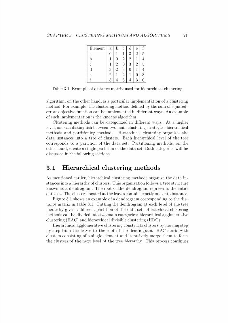
Table 3.1: Example of distance matrix used for hierarchical clustering
algorithm, on the other hand, is a particular implementation of a clustering
method. For example, the clustering method defined by the sum of squared-errors objective function can be implemented in different ways. An exampleof such implementation is the kmeans algorithm.
Clustering methods can be categorized in different ways. At a higherlevel, one can distinguish between two main clustering strategies: hierarchicalmethods and partitioning methods. Hierarchical clustering organizes thedata instances into a tree of clusters. Each hierarchical level of the treecorresponds to a partition of the data set. Partitioning methods, on theother hand, create a single partition of the data set. Both categories will bediscussed in the following sections.
3.1 Hierarchical clustering methods
As mentioned earlier, hierarchical clustering methods organize the data in-stances into a hierarchy of clusters. This organization follows a tree structureknown as a dendrogram. The root of the dendrogram represents the entiredata set. The clusters located at the leaves contain exactly one data instance.
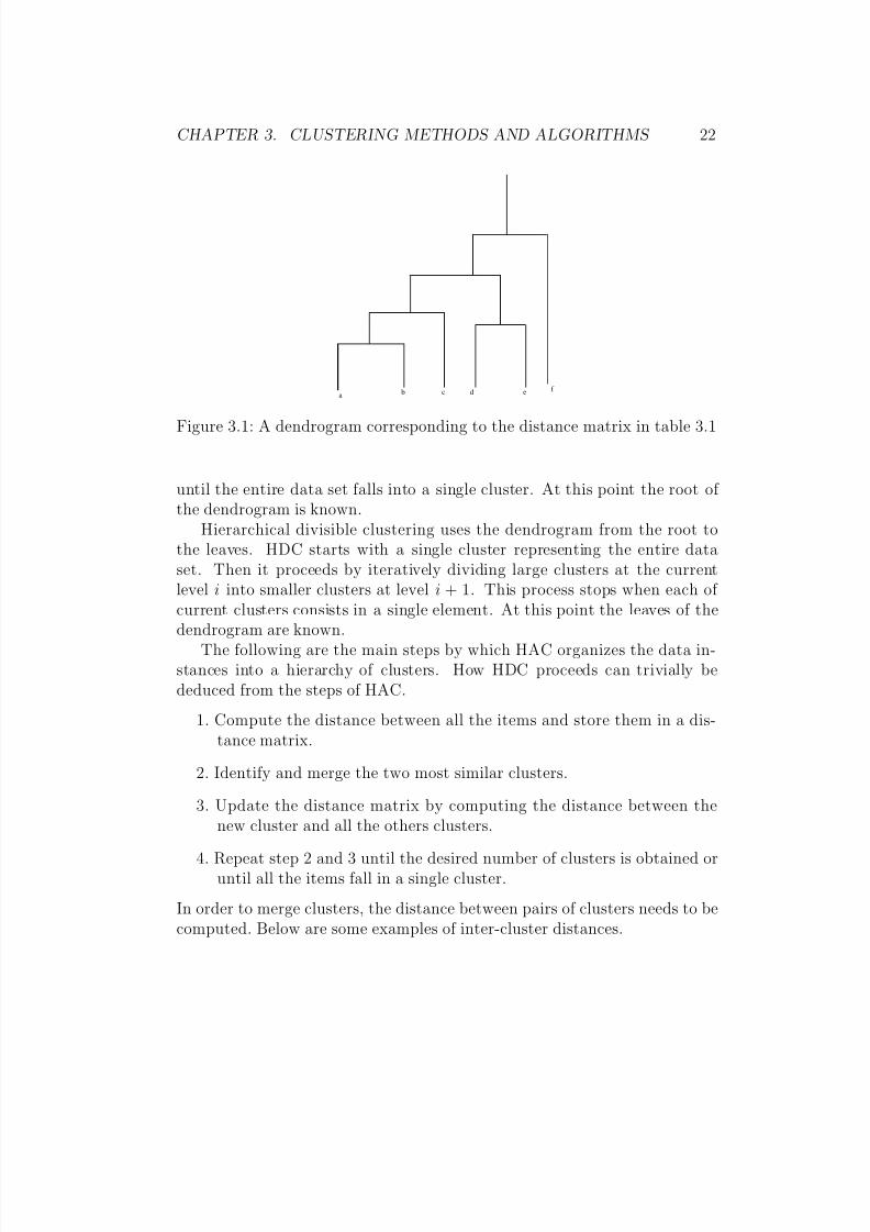
Figure 3.1 shows an example of a dendrogram corresponding to the dis-tance matrix in table 3.1. Cutting the dendrogram at each level of the treehierarchy gives a different partition of the data set. Hierarchical clustering
methods can be divided into two main categories: hierarchical agglomerativeclustering (HAC) and hierarchical divisible clustering (HDC).Hierarchical agglomerative clustering constructs clusters by moving step
by step from the leaves to the root of the dendrogram. HAC starts withclusters consisting of a single element and iteratively merge them to formthe clusters of the next level of the tree hierarchy. This process continues
8/8/2019 Comp of Clustering Method
http://slidepdf.com/reader/full/comp-of-clustering-method 31/117
CHAPTER 3. CLUSTERING METHODS AND ALGORITHMS 22
ba
df
ec
Figure 3.1: A dendrogram corresponding to the distance matrix in table 3.1
until the entire data set falls into a single cluster. At this point the root of the dendrogram is known.
Hierarchical divisible clustering uses the dendrogram from the root tothe leaves. HDC starts with a single cluster representing the entire dataset. Then it proceeds by iteratively dividing large clusters at the currentlevel i into smaller clusters at level i + 1. This process stops when each of
current clusters consists in a single element. At this point the leaves of thedendrogram are known.The following are the main steps by which HAC organizes the data in-
stances into a hierarchy of clusters. How HDC proceeds can trivially bededuced from the steps of HAC.
1. Compute the distance between all the items and store them in a dis-tance matrix.
2. Identify and merge the two most similar clusters.
3. Update the distance matrix by computing the distance between the
new cluster and all the others clusters.
4. Repeat step 2 and 3 until the desired number of clusters is obtained oruntil all the items fall in a single cluster.
In order to merge clusters, the distance between pairs of clusters needs to becomputed. Below are some examples of inter-cluster distances.
8/8/2019 Comp of Clustering Method
http://slidepdf.com/reader/full/comp-of-clustering-method 32/117
CHAPTER 3. CLUSTERING METHODS AND ALGORITHMS 23
Inter-cluster distances for hierarchical clusteringFour distances are frequently used for measuring the similarity of two clustersin hierarchical clustering. Let C 1 and C 2 be two clusters, the four inter-clusterdistances are:
• The maximum distance between C 1 and C 2:
distmax(C 1, C 2) = max( p1∈C 1, p2∈C 2)dist( p1, p2) (3.1)
• The minimum distance between C 1 and C 2:
distmin(C 1, C 2) = min( p1∈C 1, p2∈C 2)dist( p1, p2) (3.2)
• Average distance:the average of the distances of all pair of elements ( p1 ∈ C 1, p2 ∈ C 2)
• The distance between the mean µ1 of C 1 and the mean µ2 of C 2:
distmean(C 1, C 2) = dist(µ1, µ2) (3.3)
In these expressions, dist is the distance measure used between pairs of elements. Generally, euclidean distance is used.
In [3], the authors illustrate the difference between these distances. Theyshow that if the clusters are compact and non-overlapping, these distancesare similar. But in the case that the clusters overlap or are not hyperspher-ical shapes, they give results that differ significantly. The distmean is lesscomputationally expensive than the others three distance measures becauseit does not compute the distance between all pairs of instances of the twoclusters C 1 and C 2. These inter-cluster distance measures correspond to dif-ferent strategies for merging clusters. When distmin is used, the algorithmis known as the nearest-neighbor algorithm and when distmax is used, thealgorithm is called the farthest-neighbor algorithm.
The problem with hierarchical clustering is that it is computationallyexpensive both in time and space because the distances between all pairsof instances of the data set need to be computed and stored. The timecomplexity of HAC is at least O(N 2 log N ), where N is the size of the data set.This is because there is at least log N levels in the dendrogram and each of
8/8/2019 Comp of Clustering Method
http://slidepdf.com/reader/full/comp-of-clustering-method 33/117
CHAPTER 3. CLUSTERING METHODS AND ALGORITHMS 24
the requires O(N 2) for creating a partition. Because of its high computation
time, hierarchical clustering are not suitable for clustering large data sets.Hierarchical clustering algorithms do not aim at maximizing a global
objective function. At each step of the clustering process, they make localdecisions in order to find the best way of clustering the data.
In this section, hierarchical clustering has been briefly discussed. Hierar-chical clustering is impractical for large data sets. The next section is aboutpartitioning clustering.
3.2 Partitioning clustering methods
Partitioning clustering methods, as opposed to hierarchical clustering meth-ods create a single partition of the data set. The main categories of parti-tioning clustering methods are described in the following.
3.2.1 Squared-error clustering
The objective of squared-error clustering is to find the partition of the dataset with the minimal sum of squared-errors. The squared-error of a clusteris defined as the sum of the squared euclidean distance of each of the clustermembers to the cluster’s centre. And the sum of squared-errors of a parti-
tion P = {C 1,..,C K } is defined as the sum of the squared-errors of all theclusters. In other words:
SS E (P ) =K
k=1
x∈C k
||x − µk||2, where
µk is the mean of cluster C k
µk =1
|C k|
x∈C k
x
(3.4)
The general form of a squared-error clustering is:Given a data set D,
8/8/2019 Comp of Clustering Method
http://slidepdf.com/reader/full/comp-of-clustering-method 34/117
CHAPTER 3. CLUSTERING METHODS AND ALGORITHMS 25
1. Initialisation
(a) Specify the number of clusters and assign arbitrarily each instanceof the data set to a cluster
(b) Compute the centre for each cluster
2. Iterations: Repeat steps 2a, 2b and 2c until the difference of two con-secutive iterations is below a specified threshold.
(a) Assign each instance of D to the cluster which centre it is closestto
(b) Compute the new centre for each cluster
(c) Compute the squared-error.
Why do the squared-error clustering algorithm converge?The sum of squared-errors clustering is an example of optimisation algorithmsbased on local iterative optimisation steps. Here follows the description of alocal search algorithm and the proof of its convergence.
Local search algorithm: Let P be a finite set of possible solutions (inpartitioning clustering P is the set of all partitions), and let f : P → Rbe a function to be minimized (in sum of squared clustering f is the sum of
squared errors). The algorithm starts from an initial solution x0 ∈ P . Itthen finds a minimizer x1 ∈ P of f in a neighbourhood of x0. If x1 = x0,a minimizer x2 ∈ P of f is found in a neighbourhood of x1. A sequence of minimizers x0, x1,...,xt ∈ P is constructed in this way. The iterations stopwhen xt gets very close to xt−1.
Proof: It is clear that f (x0) ≥ f (x1) ≥ ... ≥ f (xt). And the stoppingcriterion, xt = xt−1 is satisfied at the point where f (xt) = f (xt−1). Thismeans that the inequalities that exist before the stopping criterion is metare all strict, so the algorithm progresses. It stops at some point in time be-
cause D is a finite set. The convergence is local and not optimal because thealgorithm performs locally; only a subset of the solution space is investigated.
More precisely, squared-error clustering is based on a version of a localsearch algorithm called alternating minimization [20]. Alternating minimiza-tion is appropriate in situations where:
8/8/2019 Comp of Clustering Method
http://slidepdf.com/reader/full/comp-of-clustering-method 35/117
CHAPTER 3. CLUSTERING METHODS AND ALGORITHMS 26
•the variables of the function to be optimised fall in two or more groups,
• and if optimising the function by keeping some of the variables constantis easier than doing the optimisation with all the variables at the time.
The alternating minimization proceeds in the following way:Let xt = (ct,sset) be two groups of variables. In the case of squared-errorclustering, these variables are respectively the centres of the clusters and thesum of squared-errors. At each iteration t, the minimization occurs by keep-ing constant sset. ct+1 is then found as the value of c that minimizes thefunction f (c,sset). The value of sset+1 is the value of sse that minimizesf (ct+1,sse).
The main strengths of squared-error clustering are its simplicity and effi-ciency. Some of its limitations are:
• The sum of squared-errors criterion is appropriate in situations wherethe clusters are compact and non-overlapping.
• The partition with the lowest SS E is not always the one that revealsthe true structure of the data. Sometimes partitions consisting in largeclusters has smaller sum of squared error than partition that reflectsthe true structure of the data. This situation often occurs when thedata contains outliers.
One of the most popular examples of squared-error clustering is thekmeans-algorithm.
The kmeans-algorithm
Kmeans is an iterative clustering algorithm which moves items among clus-ters until a specified convergence criterion is met. Convergence is reachedwhen only very small changes are observed between two consecutive itera-tions. The convergence criterion can be expressed in terms of the sum of squared-errors but it does not need to be so expressed.
Algorithm: kmeans-algorithmInput: A data set D of size N and the number of clusters K ,Output: a set of K clusters with minimal sum of squared-error.
1. Randomly choose K instances from D as the initial cluster centres;
Repeat steps 2 and 3 until no change occurs.

8/8/2019 Comp of Clustering Method
http://slidepdf.com/reader/full/comp-of-clustering-method 36/117
CHAPTER 3. CLUSTERING METHODS AND ALGORITHMS 27
2. Assign each instance to the cluster, which centre the instance is closest
to;
3. Recompute the cluster centres. The centre of the cluster C k, is givenby:µk = 1
|C k|
j∈C kxkj , where |C k| is the size of the C k.
Kmeans is simple and efficient. Because of these qualities, kmeans iswidely used as a clustering tool.The problems associated with kmeans are mainly those common to squared-error clustering: the clustering’s result is not optimal and the sum of squared-errors is not always a good indicator of the quality of the clustering. The
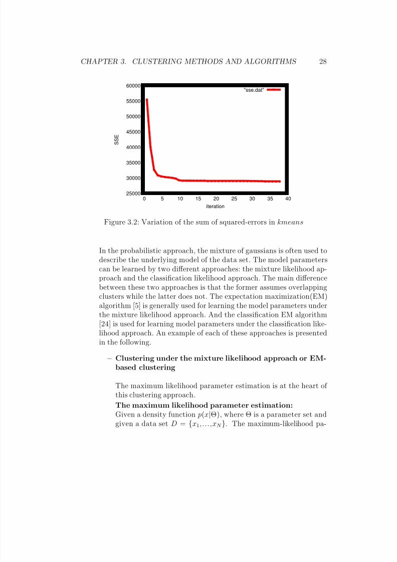
number of clusters needs to be specified by the user and the quality of theclustering is dependent on the initial values. It is appropriate when the clus-ters are compact, well separated, spherical and approximately of similar size.The algorithm does not explicitly handle outliers and the presence of outlierscan degrade the quality of the clustering. The time complexity of kmeans isO(I ∗K ∗N ), where N is the size of the data set, I is the number of iterationsand K is the number of clusters. Generally, the maximum number of itera-tions is specified. In these cases, the time complexity is O(K ∗ N ). Figure3.2 illustrates how the sum of squared-errors varies during the iterations of the kmeans algorithm.
Figure 3.2 shows that the sum of squared-errors decreases very slowlyafter the 10th iteration. This indicates that convergence of the kmeans isreached around the 10th iteration.
3.2.2 Model-based clustering
Model-based clustering methods assume that the data set has an underly-ing mathematical model, and they aim at uncovering this unknown model.Generally, the model is specified in advance and what remains is the compu-tation of its parameters. Two main classes of model-based clustering exist.The first class is based on a probabilistic approach and the second is basedon an artificial neural networks approach.
• Probabilistic clustering
8/8/2019 Comp of Clustering Method
http://slidepdf.com/reader/full/comp-of-clustering-method 37/117
CHAPTER 3. CLUSTERING METHODS AND ALGORITHMS 28
25000
30000
35000
40000
45000
50000
55000
60000
0 5 10 15 20 25 30 35 40
S S E
iteration
"sse.dat"
Figure 3.2: Variation of the sum of squared-errors in kmeans
In the probabilistic approach, the mixture of gaussians is often used todescribe the underlying model of the data set. The model parameterscan be learned by two different approaches: the mixture likelihood ap-proach and the classification likelihood approach. The main differencebetween these two approaches is that the former assumes overlappingclusters while the latter does not. The expectation maximization(EM)algorithm [5] is generally used for learning the model parameters underthe mixture likelihood approach. And the classification EM algorithm[24] is used for learning model parameters under the classification like-lihood approach. An example of each of these approaches is presentedin the following.
– Clustering under the mixture likelihood approach or EM-based clustering
The maximum likelihood parameter estimation is at the heart of this clustering approach.
The maximum likelihood parameter estimation:Given a density function p(x|Θ), where Θ is a parameter set andgiven a data set D = {x1,...,xN }. The maximum-likelihood pa-
8/8/2019 Comp of Clustering Method
http://slidepdf.com/reader/full/comp-of-clustering-method 38/117
CHAPTER 3. CLUSTERING METHODS AND ALGORITHMS 29
rameter estimation consists in finding the value Θmax of the pa-
rameter Θ that maximizes the likelihood function λ defined as:
M (D|Θ) = ΠN n=1 p(xn|Θ) = λ(Θ|D), (3.5)
For the purpose of identifying clusters in a data set, the densityfunction used is a mixture of density functions. Each componentof the mixture represents a cluster.The mixture of density functions is defined as:
∀x
∈D, p(x
|Θ) =
K
k=1
αk p(x
|Θk)) (3.6)
where Θ = (Θ1, ..., ΘK )t is a set of parameters and
K k=1 αk = 1.
p(x|Θk) and αk are respectively the density function and the mix-ture proportion of the kth mixture component.
The maximum likelihood parameter estimation approach is basedon two assumptions:For a specified value of the parameter Θ,- the instances xi of the data set D are statistically independent- the selection of instances from a mixture component is done in-
dependently of the other components.An intuitive way of explaining the selection of each instance xi inthe mixture model is that it happens in two steps:-firstly by selecting a component k with probability αk,-and secondly by selecting xi from the component k with the prob-ability p(x|Θk).
For the experiments in this thesis, the model used is the mixtureof isotropic gaussians. This model is also known as the mixtureof spherical gaussians. In this model, each component of the mix-
ture is a spherical gaussian. The mixture of isotropic gaussianshas been chosen because of its simplicity, efficiency and scalabilityto higher dimension.The EM algorithm is a general method, used for estimating theparameters of the mixture model. It is an iterative procedure thatconsists in two steps: the expectation step and the maximization
8/8/2019 Comp of Clustering Method
http://slidepdf.com/reader/full/comp-of-clustering-method 39/117
CHAPTER 3. CLUSTERING METHODS AND ALGORITHMS 30
step. The expectation step is commonly called the E-step and the
maximization step is called the M-step. The E-step estimates theextent to which instances belong to clusters. The M-step computesthe new parameters of the model on the basis of the estimates of the E-step. In the case of the mixture of isotropic gaussians, themodel parameters are the means, standard deviations and theweights of the clusters. This step is called the maximization stepbecause it finds the values of the parameters that maximize thelikelihood function.The E and M steps are repeated until convergence of the parame-ters is reached. Convergence is reached when the parameter values
of two consecutive iterations get very close. At the end of the it-erations, a partitioning of the data set is obtained by assigningeach data instance to the cluster to which the instance has high-est membership degree. This way of assigning instances to clustersis called the maximum a posteriori (MAP) assignment. MAP as-signment gives a crisp or hard clustering of the data set. A softclustering -also called fuzzy clustering- can be obtained by usingthe cluster membership degrees computed in the E-step.
8/8/2019 Comp of Clustering Method
http://slidepdf.com/reader/full/comp-of-clustering-method 40/117
CHAPTER 3. CLUSTERING METHODS AND ALGORITHMS 31
Algorithm: Learning a mixture of isotropic gaussians with
the EM algorithmInput: the data set of size N, a set of parameters Θ for the mixtureof gaussians: Θ = {αk, µk, σk}k=1,...,K
Output: A partition of the data set into K clusters: {C 1,...,C K }
1. Random initialisation of the parameter set Θ
2. Repeat steps 3 and 4 until the log-likelihood functionlog(λ(Θ |D)) converges
3. E-step: Estimation of the posterior probabilities of the kth com-ponent.P (k|xn, Θ) = αkγ (xn|θk)
jαjγ (xn|θj)
where γ (xn|θk) = 1(√2πσk)d
exp(−xn−µk22σ2
k
)
4. M-step: Re-estimation of the parameter set Θ of the model
µ(new)k =
n
P (k|xn,Θ)xnn
P (k|xn,Θ),
σ(new)k = 1dn
P (k|xn,Θ)xn−µ(new)k
2
n
P (k
|xn,Θ)
,
α(new)k = 1
N
n P (k|xn, Θ)
5. MAP assignment of instances to clustersIn the rest of this section about EM-based clustering, we will ex-plain how the expressions of the model parameters used in theiterations of the EM algorithm are obtained.
How does the EM algorithm work?This section constitutes preparatory remarks concerning the EM
algorithm. Estimating the parameters of the mixture model usingthe maximum likelihood approach can be difficult or easy depend-ing on the expression of likelihood function. In simple cases, theproblem can be solved by computing the derivative of the likeli-hood function with respect to the model parameters. The valueof the parameters that maximize the likelihood function are then
8/8/2019 Comp of Clustering Method
http://slidepdf.com/reader/full/comp-of-clustering-method 41/117
CHAPTER 3. CLUSTERING METHODS AND ALGORITHMS 32
found by setting the derivative to zero. In most cases, the problem
is not easy and special techniques, such as the EM algorithm areneeded to solve it. The EM algorithm can be explained in vari-ous ways. In the following, we interpret EM approach as a lowerbound maximization problem. This approach has been presentedin [26]. In this approach, the maximization of the complex log-likelihood expression is replaced by the maximization of a simplerlower bound function.
Here follows a brief explanation for why maximizing the boundfunction helps maximizing the log-likelihood function. One of theconstraints the lower bound function must satisfy is that it must
touch the log-likelihood function at the current estimate of themaximizer. Given that constraint and given two functions g andh, let y = arg maxxg(x). Suppose that g(x) ≤ h(x) ∀x, and forsome z, g(z) = h(z). Then, if g(y) > g(z) then, h(y) > h(z). Thismeans that a maximizer of g is also a maximizer of h. (Here, zis the current estimate of maximizer of h and y is its new estimate).
Computation of the model parametersAs mentioned earlier, the mixture model of interest is the mixtureof isotropic gaussians(MIXIG) and its parameters are {αk, µk, σk}1≤k≤K .
The parameters {αk, µk, σk} are respectively the mixture propor-tion, the mean and the standard deviation of the kth mixturecomponent. In this section, the expressions used for computingthe new estimates of the parameters at each iteration of EM pro-cess will be derived.In the E-step, the posterior probabilities for the tth iteration arecomputed. The posterior probabilities express the membershipdegree of instances to clusters. The membership degree of in-stance xn to the kth cluster, given the current parameters Θ(t) =
(Θ(t)1 , ..., Θ
(t)K ) is: P (t)(k|xn, Θ(t)) =
α(t)k
γ (xn|Θ(t)k)
N
j=1α(t)j γ (xn|Θ(t)
j )
The denominator of this fraction ensures that the sum of the pos-teriors in each iteration gives 1. The numerator expresses how theinstance xn is selected from the data set: first a cluster is cho-sen with a probability αk and then xn is selected from the chosencluster according to the density function governing the selectedcluster; this gives the value αkγ (xn|Θ(t)
k ).
8/8/2019 Comp of Clustering Method
http://slidepdf.com/reader/full/comp-of-clustering-method 42/117
CHAPTER 3. CLUSTERING METHODS AND ALGORITHMS 33
The density function for each of the cluster is an isotropic gaus-
sian. And its expression is:
γ (xn|Θ(t)k ) = 1
(√2Πσ
(t)k)d
exp−12
xn−µ(t)k 2
(σ(t)k
)2 , where Θ(t)k = (µ(t)
k , σ(t)k )
In the following, we find a lower bound function of the log-likelihoodfunction.Let us recall the likelihood function; it is given by:λ(Θ|D) =
N n=1 h(xn|Θ), where the function h is the gaussian mix-
ture density function. By definition h(x|Θ) =K
k=1 αkγ (xn|Θk),where the function γ is the isotropic gaussian.
Putting it all together we get:
λ(Θ|D) =N
n=1
K k=1
αkγ (xn|Θk) (3.7)
The logarithm of λ is easier to manipulate than λ. Because thefunction log λ varies the same way as the function λ does, max-imizing log λ is the same as maximizing λ. The logarithm of λ,called the log-likelihood function is:δ(Θ|D) = log λ(Θ|D) =
N n=1 log(
K k=1 αkγ (xn|Θk))
This expression is complex and difficult to maximize because of the logarithm of a sum it contains. Therefore, a lower boundfunction of this function will be found and maximized instead. Inorder to make the manipulation of symbols easier, some notationsare here introduced: s(k, n) = αkγ (xn|Θk); that gives:δ(Θ|D) =
N n=1 log(
K k=1 s(k, n))
δ(Θ|D) =N
n=1 log(K
k=1 P (t)(k|xn, Θ) s(k,n)P (t)(k|xn,Θ)
)
And using Jensens inequality [appendix D.2], this gives
δ(Θ|D) ≥n k
P (t)(k|xn, Θ)log(s(k, n)
P (t)(k|xn, Θ)
) = Bt(Θ). (3.8)
By rewriting Bt(Θ), we get :
Bt(Θ) =
n
k
P (t)(k|xn, Θ)log(s(k, n))−n
k
P (t)(k|xn, Θ)log(P (t)(k|xn, Θ)
(3.9)
8/8/2019 Comp of Clustering Method
http://slidepdf.com/reader/full/comp-of-clustering-method 43/117
CHAPTER 3. CLUSTERING METHODS AND ALGORITHMS 34
From the E-step, the second term of the right side of this expres-
sion is known, therefore the maximization Bt(Θ) is reduced to themaximization of
bt(Θ) =
n
k
P (t)(k|xn, Θ)log(s(k, n)) (3.10)
This results in the following formulas:The formulas are obtained by computing the derivative of thelower bound function with respect to each of the parameters of the model and by setting each of these derivatives to zero.Here are the details of the derivation of the formulas of the modelparameters.Formula of the mean:
∂bt(Θ)
∂µk
=N
n=1
P (t)(k|xn, Θ)µk − xn
σ2k
= 0 (3.11)
Which gives
µ(t+1)k =
n P (t)(k|xn, Θ)xn
n P (t)(k|xn, Θ)(3.12)
The computation of the standard deviation is obtained in the sameway. First, µ
(t+1)k is inserted in bt(Θ) and then bt(Θ) is derived with
respect to σk. This gives the expression:
σ(t+1)k =
1
d
n P (t)(k|xn, Θ)xn − µ
(t+1)k 2
n P (t)(k|xn, Θ)(3.13)
For the derivation of the expression of the mixture probabilities,the constraint
k αk = 1 must be considered. In order to do
this, the lagrange method [D.3], is used. The expression bt(Θ) isextended by including the constraint
k αk = 1. This results in a
new function:
f t(Θ) = bt(Θ) + λ(K
k=1
αk
−1), (3.14)
where λ is the lagrange multiplier. By inserting the expression of bt(Θ), this gives:
f t(Θ) =
n
k
P (t)(k|xn)log(s(k, n)) + λ(K
k=1
αk − 1), (3.15)
8/8/2019 Comp of Clustering Method
http://slidepdf.com/reader/full/comp-of-clustering-method 44/117
CHAPTER 3. CLUSTERING METHODS AND ALGORITHMS 35
where
s(k, n) = αkγ (xn|Θk) = αk
1
(√
2Πσ(t)k )d
exp
−12
xn−µ(t)k 2
(σ(t)k
)2 (3.16)
Setting the derivative of f t(Θ) with respect to αk to zero gives:
∂f t(Θ)
∂αk
=N
n=1
P (t)(k|xn, Θ)(1
αk
) + λ = 0 (3.17)
Which gives:
αk = −N
n=1 P (t)
(k|xn, Θ)λ
(3.18)
By taking into account the constraintK
k=1 αk = 1, we get:
1 =K
k=1
αk =−K
k=1
N n=1 P (t)(k|xn, Θ)
λ(3.19)
This is equivalent to:
1 =−
N n=1
K k=1 P (t)(k|xn, Θ)
λ
=
−
N
λ
, (3.20)
becauseK
k=1 P (t)(k|xn, Θ) = 1Which means
λ = −N (3.21)
Replacing λ by its value in the equation 3.18 gives the estimate of the mixing probability:
α(t+1)k =
1
N
n
P (t)(k|xn, Θ). (3.22)
In this section, we have discussed one example of probability-basedclustering that uses the mixture likelihood approach. This ap-proach assumes that clusters overlap. The next section is anotherexample of probabilistic clustering. It is based on the classifica-tion likelihood approach. This approach assumes that the clustersare non-overlapping.
8/8/2019 Comp of Clustering Method
http://slidepdf.com/reader/full/comp-of-clustering-method 45/117
CHAPTER 3. CLUSTERING METHODS AND ALGORITHMS 36
– Clustering under the classification likelihood approach or
CEM-based clusteringThe objective of clustering under the classification likelihood ap-proach is to find a partition of the data set that maximizes theclassification likelihood criterion κ defined as:
κ(Θ|D) =K
k=1
xik∈Ck
log(αk p(xik|µk, σk)) (3.23)
C k is the kth cluster and µk, σk, αk are respectively its mean,standard deviation and mixture proportion.
While the EM algorithm is a general method for estimating themodel parameters under the mixture approach, the classificationEM is a method for estimating the model parameters under theclassification approach. The classification EM algorithm has beenproposed by G. Celeux and G. Govaert in [24].
The classification likelihood objective criterion κ is a special caseof the mixture likelihood criterion. In this special case, each in-stance belongs exclusively to a single cluster. Like the EM al-gorithm, the classification EM algorithm has an expectation step
and a maximization step. During the expectation step, the ex-pected membership degree of each instance to each of the clustersis computed. Using the cluster membership degrees, computed inthe E-step, the maximization step computes the values of the pa-rameters that maximize the log-likelihood function. In addition,the classification EM algorithm has a classification step, calledC-step. The C-step takes place between the E-step and the M-step. In the classification step, instances are assigned to clustersaccording to the maximum a posteriori (MAP) principle. Belowis a description of the classification EM algorithm:
8/8/2019 Comp of Clustering Method
http://slidepdf.com/reader/full/comp-of-clustering-method 46/117
CHAPTER 3. CLUSTERING METHODS AND ALGORITHMS 37
Algorithm: learning model parameters via CEM algorithm
InputA dataset set D of size N, the desired number of cluster K
Output A partition of D in K clusters.
1. InitialisationStart from an initial partition P 0 of the data set.
Repeat the E, C and M steps until convergence is reached.
2. E-step: Computation of the posterior probabilities:For i = 1,...,N and for k = 1,...,K , the posterior probability
zik for data instance xi belonging to cluster C k is given byz(t+1)ik =
α(t)k
f (xi,Θ(t)k)K
r=1α(t)r f (xi,Θ
(t)r )
, where α(t)k and Θ
(t)k are the values
of the parameters of the model at the tth iteration and f is adensity distribution function.
3. C-step: MAP assignment of items to clusters
4. M-step: Computation of the parameter valuesFor k = 1,...,K , α(t+1)
k = N kN
, where N k is the size of C k.The formula for the computation of the parameter Θk dependson the exact expression of f .In this thesis, f is a mixture of isotropic gaussians.The mean of the cluster k is µk and its variance is σk.This gives the expression:µ(t+1)
k = 1N k
xi∈C
(t)k
xi, ∀k = 1,...,K
and
(σk)(t+1) =
1
N kd
xi∈C
(t)k
xi − µ(t+1)k
2, where d is the dimen-
sion of the data space and N k is the size of cluster C k.
These formula are intuitive. As a special case of the mixture like-lihood, these formula can be derived from that of the EM-basedapproach. This is done by replacing, P (t)(k|xn, Θ) respectivelywith 1 if xn ∈ C k and with 0 if xn /∈ C k in the formula obtainedwith the EM algorithm.
Figure 3.3 shows how the log-likelihood of the data increases with
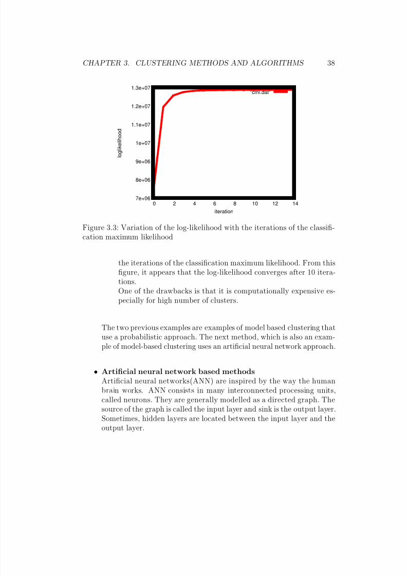
8/8/2019 Comp of Clustering Method
http://slidepdf.com/reader/full/comp-of-clustering-method 47/117
CHAPTER 3. CLUSTERING METHODS AND ALGORITHMS 38
7e+06
8e+06
9e+06
1e+07
1.1e+07
1.2e+07
1.3e+07
0 2 4 6 8 10 12 14
l o g l i k e l i h o o d
iteration
"cml.dat"
Figure 3.3: Variation of the log-likelihood with the iterations of the classifi-cation maximum likelihood
the iterations of the classification maximum likelihood. From thisfigure, it appears that the log-likelihood converges after 10 itera-tions.
One of the drawbacks is that it is computationally expensive es-pecially for high number of clusters.
The two previous examples are examples of model based clustering thatuse a probabilistic approach. The next method, which is also an exam-ple of model-based clustering uses an artificial neural network approach.
• Artificial neural network based methodsArtificial neural networks(ANN) are inspired by the way the humanbrain works. ANN consists in many interconnected processing units,called neurons. They are generally modelled as a directed graph. Thesource of the graph is called the input layer and sink is the output layer.Sometimes, hidden layers are located between the input layer and theoutput layer.
8/8/2019 Comp of Clustering Method
http://slidepdf.com/reader/full/comp-of-clustering-method 48/117
CHAPTER 3. CLUSTERING METHODS AND ALGORITHMS 39
ANN are used for both classification and clustering. They can be com-
petitive or non-competitive. In competitive learning, the output nodescompete and only one of them wins. A commonly used competitiveapproach for clustering is self-organizing maps (SOM). The term self-organizing refers to the ability of the nodes of the networks to organizethemselves into clusters.
SOM are represented by a single layered neural network in which eachoutput node is connected to all input nodes. This is illustrated in figure3.4. When an input vector is presented to the input layer, only a sin-gle output node is activated. This activated node is called the winner.When the winner has been identified its weights are adjusted. At the
end of the learning process, similar items get associated to the sameoutput node. The most popular examples of SOM are the Kohonenself-organizing maps [47].
Kohonen Self-Organizing Maps(SOM) algorithm
Kohonen self-organizing maps were developed by Teuvo Kohonen around1982. They have two layers: an input layer and a competitive layer, asillustrated in figure 3.4. The competitive layer is a grid of nodes. Eachinput node is connected to all the nodes in the competitive layer. Thelinks between the input nodes and the nodes of the competitive layerhave a weight, and each node in the competitive layer has an activa-tion function. The network learns in the following way: initially, theweights of the network are randomly initialised. Then for each inputvector presented to the input layer, each of the competitive nodes pro-duces an output value. The node that produces the best output valueis the winner of the competition. As a result, the weights of the winnernode as well as those of the nodes in its neighbourhood are adjusted.
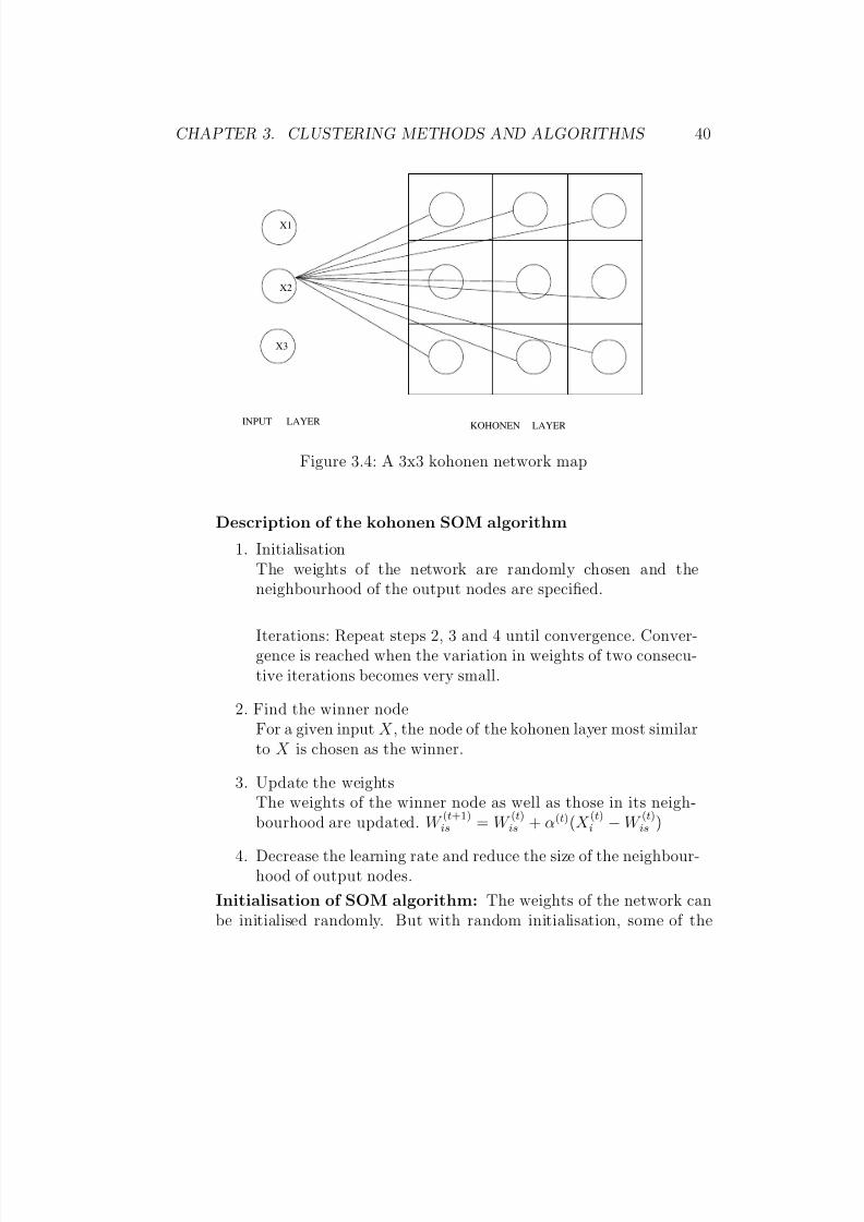
8/8/2019 Comp of Clustering Method
http://slidepdf.com/reader/full/comp-of-clustering-method 49/117
CHAPTER 3. CLUSTERING METHODS AND ALGORITHMS 40
INPUT LAYER
X1
X2
X3
KOHONEN LAYER
Figure 3.4: A 3x3 kohonen network map
Description of the kohonen SOM algorithm
1. InitialisationThe weights of the network are randomly chosen and theneighbourhood of the output nodes are specified.
Iterations: Repeat steps 2, 3 and 4 until convergence. Conver-gence is reached when the variation in weights of two consecu-tive iterations becomes very small.
2. Find the winner nodeFor a given input X , the node of the kohonen layer most similarto X is chosen as the winner.
3. Update the weightsThe weights of the winner node as well as those in its neigh-
bourhood are updated. W (t+1)is = W (t)is + α(t)(X (t)i − W (t)is )
4. Decrease the learning rate and reduce the size of the neighbour-hood of output nodes.
Initialisation of SOM algorithm: The weights of the network canbe initialised randomly. But with random initialisation, some of the
8/8/2019 Comp of Clustering Method
http://slidepdf.com/reader/full/comp-of-clustering-method 50/117
CHAPTER 3. CLUSTERING METHODS AND ALGORITHMS 41
output nodes may never win the competition. This problem can be
avoided by randomly choosing instances of the data set as initial val-ues of the weights.
Choice of distance measure: The dot product and the euclideandistance are commonly used as distance measures. The dot product isused in situations where the input patterns and the network weightsare normalized.
Learning rate: The learning rate controls the amount by which theweights of the winner node and that of its neighbours are adjusted. Theinitial learning rate is specified at the initialisation. Then it decreasesas the number of iterations increases. Decreasing the learning rateensures that the learning process stops at some point in time. Thisis important because usually the convergence criterion is defined interms of very small changes in the weights of two consecutive iterations.Competitive learning does not give any guaranties that this convergencecriteria will eventually be satisfied.
Defining the neighbourhood: Initially, the neighbourhood is set toa large value which then decreases with the iterations. This correspondsto assigning instances to nodes with more precision as the number of iterations increases.
The time complexity of SOM is O(M ∗ N ), where M is the size of thegrid and N is the size of the data set. The justification of this timecomplexity is the following: during the training a number of operations(finding the winner and updating the neighbourhood), which is are atmost twice the size of the grid take place. And the maximum numberof iterations is equal to the size of the data. So the time complexityfor the training is O(M ∗ N ). As the assignment only takes O(N ) thisgives a total complexity of O(M ∗ N ).
One of the main strengths of SOM is its ability to preserve the topologyof the input data: items that are close to each other in the input space
remain close in the output space. This makes SOM a valuable tool forvisualizing high dimensions data in low dimension. SOM also supportsparallel processing; this can speed up the learning process.
Some of the limitations of Kohonen SOM are: it is most appropriatefor detecting hyperspherical clusters. The choice of initial parametervalues - the initial weights of connections, the learning rate, and the
8/8/2019 Comp of Clustering Method
http://slidepdf.com/reader/full/comp-of-clustering-method 51/117
CHAPTER 3. CLUSTERING METHODS AND ALGORITHMS 42
size of the neighbourhood - is difficult. The quality of the clustering
depends on the choice of the initial values of these parameters and alsoon the order in which items are processed.
This subsection has discussed model-based clustering. This approachassumes that the data can be described by a mathematical model andaim at uncovering this model. The two main approaches to model-based clustering are the probabilistic approach and the artificial neuralnetwork approach. The next subsection approaches the clustering prob-lem differently. It views clusters as dense regions in the data space.
3.2.3 Density-based clusteringIn the density-based approach, a cluster is defined as a region of thedata space with high density. This dense region is bordered by low-density regions that separate the cluster from other points of the dataspace. There are two main types of density-based clustering: the ap-proach based on connectivity and the approach based on density func-tions. An example of a clustering algorithm based on connectivity isDBSCAN [46] and an example based on density functions is DENCLUE[27]. These two algorithms are popular for clustering large spatial datasets.
The two algorithms will be briefly presented in the following.
1. DBSCAN: Density-Based Spatial Clustering using Appli-cations with NoiseDBSCAN finds clusters by first identifying points in dense regionsand then growing the regions around these points until the bor-ders of these regions are met. To be more specific, DBSCAN findsclusters by:- First identifying core points of the data set. A core point is apoint whose neighbourhood contains a minimum number of points.
The size of the neighbourhood and the the minimum number of points are two parameters of the algorithm.- Next, DBSCAN iteratively merges core points that are directlydensity-reachable. A point p is directly density-reachable from apoint q if q is a core point and p belongs to the neighbourhood of q. The iterations stop when it is no longer possible to add new
8/8/2019 Comp of Clustering Method
http://slidepdf.com/reader/full/comp-of-clustering-method 52/117
CHAPTER 3. CLUSTERING METHODS AND ALGORITHMS 43
points to any of the clusters. DBSCAN is designed for spatial data
sets. A spatial data set capture the spatial relationship betweenthe instances of the data set. Examples of spatial data sets aregeographical data sets or image databases. The time complexityof DBSCAN is O(N log N ) when the spatial index R∗-tree is used.Some of the difficulties in using DBSCAN are related to the choiceof appropriate values of the neighbourhood and the minimumnumber of points that characterizes a core point.
Some of the advantages of density-based clustering are their abil-ity to detect clusters of arbitrary shapes and scalability to largedata sets.
2. DENCLUE: DENsity-based CLUstEringDENCLUE is a clustering algorithm that uses density distribu-tion functions to identify clusters. Clusters are identified as localmaxima of the overall density function. The overall density func-tion is the sum of all the influence functions of each point of thedata space. Given a data set D, the influence function of a pointy ∈ D is a function f y : D → R+
0 , which models the impact of y within a neighbourhood. The gaussian distribution function isan example of an influence function that is commonly used. The
gaussian function is defined as:f yGauss(x) = exp(−d(x,y)2
2σ2 ), where d is a distance measure.Clusters are generated by density attractors. A density attractoris a local maximum of the (overall) density function.There are two types of clusters: center-defined clusters and arbi-trary shaped clusters.Center-Defined Cluster: Given a threshold Γ, a center-definedcluster for a density attractor xmax is the subset C of the data setD defined by:C = {y ∈ D|y is density-attracted by xmax and f yβ (xmax) ≥ Γ}
Arbitrary-shaped Cluster: Given Γ, an arbitrary-shaped clus-ter for the set of density attractors A is a subset C of the data setD, such that:- ∀x ∈ C , ∃ xmax ∈ A with f Dβ (xmax) ≥ Γ and x is density-attracted by xmax,
8/8/2019 Comp of Clustering Method
http://slidepdf.com/reader/full/comp-of-clustering-method 53/117
CHAPTER 3. CLUSTERING METHODS AND ALGORITHMS 44
- For all density attractors xmax1 and xmax
2 there is a path from
xmax1 to xmax2 such that for all points y on this path, f Dβ (y) ≥ Γ.
The notion of density-attracted points used in these two defini-tions of clusters is defined as follows:Density-attracted points: Given ∈ R+, a point x ∈ Dis density-attracted to a density attractor xmax if and only if there exists a chain of points x0, x1,...,xk such that x0 = x and
d(xk, xmax) ≤ where xi = xi−1 + δ∆f D
β(xi−1)
||∆f Dβ(xi−1)|| for 0 < i < k.
For continuous and differentiable influence functions, such as thegaussian influence function, a hill-climbing algorithm guided by
the gradient can be used to find density-attracted points. The de-scription of the hill-climbing algorithm can be found in appendixappendix D.1.
DENCLUE consider outliers as noise and remove them. Some of the strengths of DENCLUE are:-It has a solid mathematical foundation-It is good for clustering high dimensional data-It detects clusters of arbitrary shapes
The main limitations of these algorithms are they remove have
been designed for spatial data only. The fact that they removeoutliers does not them suitable for identifying attack clusters thatare small. The quality of the clustering result depends on thechoice of density parameter and the noise threshold.
This subsection has presented the density-based approach to cluster-ing. In this approach, clusters are defined as dense regions of the dataspace. Two examples of algorithms have been presented: DBSCANand DENCLUE. These algorithms are designed for spatial data. Thenext subsection discusses the grid-based approach to clustering. This
approach is also designed for spatial data. It views the data space as agrid.
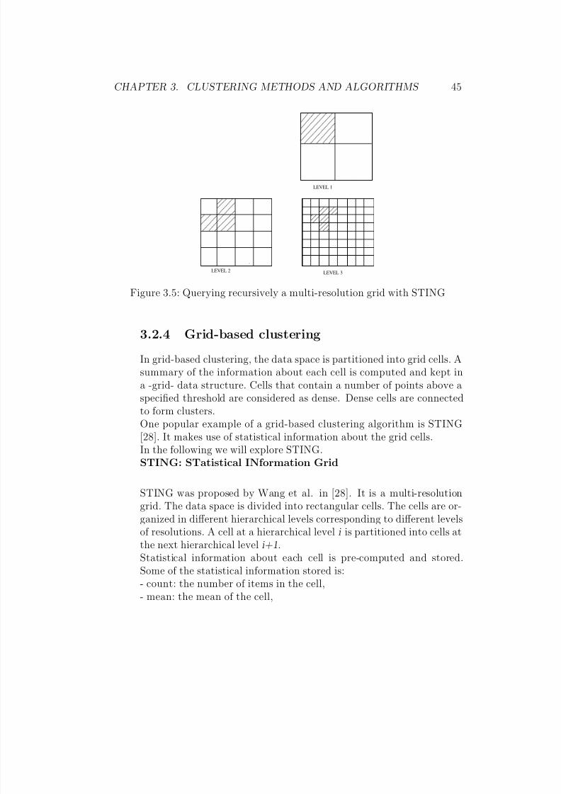
8/8/2019 Comp of Clustering Method
http://slidepdf.com/reader/full/comp-of-clustering-method 54/117
CHAPTER 3. CLUSTERING METHODS AND ALGORITHMS 45
LEVEL 3
LEVEL 1
LEVEL 2
Figure 3.5: Querying recursively a multi-resolution grid with STING
3.2.4 Grid-based clustering
In grid-based clustering, the data space is partitioned into grid cells. Asummary of the information about each cell is computed and kept ina -grid- data structure. Cells that contain a number of points above a
specified threshold are considered as dense. Dense cells are connectedto form clusters.One popular example of a grid-based clustering algorithm is STING[28]. It makes use of statistical information about the grid cells.In the following we will explore STING.STING: STatistical INformation Grid
STING was proposed by Wang et al. in [28]. It is a multi-resolutiongrid. The data space is divided into rectangular cells. The cells are or-ganized in different hierarchical levels corresponding to different levels
of resolutions. A cell at a hierarchical level i is partitioned into cells atthe next hierarchical level i+1.Statistical information about each cell is pre-computed and stored.Some of the statistical information stored is:- count: the number of items in the cell,- mean: the mean of the cell,
8/8/2019 Comp of Clustering Method
http://slidepdf.com/reader/full/comp-of-clustering-method 55/117
CHAPTER 3. CLUSTERING METHODS AND ALGORITHMS 46
- s: the standard deviation,
- min: the minimum value of the cell,- max: the maximum value of the cell,- the distribution: the distribution of the cell if it is known.Statistical information about the cells is computed in a bottom-up fash-ion. For example, the distribution at the hierarchical level i can beestimated to be the distribution of the majority of cells at the hierar-chical level i − 1.The statistical information about the cells is used in a top-down fash-ion to answer spatial queries. A query asks for the selection of cellssatisfying certain conditions on density for example.
The query-answering is performed in the following way:First the level of the cell hierarchy where the answering is to begin isfound. Generally, it contains a small number of cells. Then for eachcell at this level, the relevancy of the cell in answering the query isestimated. Only the relevant cells are submitted to further processingin the next hierarchical level down.This process is repeated until the lowest level of the hierarchy is reached.At this stage the cells satisfying the query are returned. Usually thisends the clustering process. In cases where very accurate results aredesired, the relevant cells are submitted to further processing. Onlycell members that satisfy the query are returned.
Figure 3.5 illustrates a top-down querying of the grid in STING. Start-ing at level 1, the possible candidates satisfying the query are localized.These initial solutions are refined at levels 2 and 3. The desired cellsare returned at level 3. As it appears from this figure, the borders of the cluster are either horizontal or vertical.
Some of the strengths of STING and grid based clustering in generalare: -It is scalable to a large data set. The query processing time is
linear with respect to the number of cells.-The grid structure supports parallel processing and incremental up-dating.One of the weaknesses of STING is that the borders of the clustersare either vertical or horizontal. Grid based clustering algorithms aredesigned for clustering spatial data. They will not be considered for
8/8/2019 Comp of Clustering Method
http://slidepdf.com/reader/full/comp-of-clustering-method 56/117
CHAPTER 3. CLUSTERING METHODS AND ALGORITHMS 47
the experiment as the data to be used does not capture the spatial
relationship between items.
The following two clustering methods correspond to two other waysof categorizing clustering methods. In the first of these categorizations,a distinction is made between online and off-line clustering algorithms.All the methods discussed up to now, except SOM, are off-line methods.The second categorization distinguishes between crisp clustering andfuzzy clustering. Crisp clustering creates distinct clusters, while infuzzy clustering, items belongs to more than one cluster.
3.2.5 Online clustering
One of the main differences between off-line clustering and online clus-tering is that the former requires that the entire data set is availableat each step of the clustering. That is so because off-line clusteringalgorithms generally aim at finding the global optimiser of an objectivefunction. The latter -online clustering algorithms- generates clusters asthe data is produced. Online clustering algorithms are appropriate forclustering in a data flow environment. Network traffic is an example of
such a type of data.Online clustering algorithms do not aim at optimising a global crite-rion, rather they proceed by making local decisions. Optimisation of a global criterion often leads to a stability problem, in that the clus-ters produced by these methods are sensitive to small changes in thedata. The advantage of online clustering is that it leads to adaptableand stable cluster structure. An example of online clustering is leaderclustering [31].
The leader clustering algorithm
Leader clustering starts by selecting a representative of a cluster. Thisrepresentative is called the leader of the cluster. When assigning in-stances to clusters, the distances of the instance to each of the currentclusters are computed. The instance is assigned to the closest clusterif its distance to that cluster is below a specified threshold . If the dis-tance of the instance to each of the existing clusters is greater than the
8/8/2019 Comp of Clustering Method
http://slidepdf.com/reader/full/comp-of-clustering-method 57/117
CHAPTER 3. CLUSTERING METHODS AND ALGORITHMS 48
threshold, a new cluster, consisting of that single instance, is created.
This process is repeated for each of the instances. Generally, euclideandistance is used.
Description of the algorithm
1. InitialisationChoose a threshold , and initialise the first cluster centre µ0.Generally the first item of the data set is chosen.
For each of the remaining items x repeat the following steps:
2. Identify the closest cluster C closest
3. If x − µclosest < , update the centre µclosest otherwise create anew cluster with x as its leader.
One of the main drawbacks of leader clustering, that is common toon-line clustering algorithms, is that the clustering result is dependenton the order in which instances are processed. When leader clusteringis used for off-line clustering, this problem can be solved by selectinginstances in a random order.Some of the strengths of leader clustering are: it is fast, robust to
outliers and does not require the number of clusters to be specified ex-plicitly. Its robustness in the presence of outliers indicates that it mayhave some potential for clustering network traffic data for anomaly de-tection.The time complexity of the leader clustering is O(K ∗ N ), where K is the number of clusters and N is the size of the data set. A singlescan of the data set is required and a constant number of operations isperformed during the processing of each instance.
3.2.6 Fuzzy clustering
Another way of categorizing clustering methods is to consider the de-gree of membership of data instances to clusters. A distinction is madebetween crisp clustering and fuzzy clustering. In crisp clustering, eachdata instance is assigned to only one cluster. In fuzzy clustering, on the
8/8/2019 Comp of Clustering Method
http://slidepdf.com/reader/full/comp-of-clustering-method 58/117
CHAPTER 3. CLUSTERING METHODS AND ALGORITHMS 49
other hand, each instance belongs to more than one cluster with some
degree of membership. The degree of membership of a data instanceX i to a cluster C k is a real value zik ∈ [0, 1], where
k zik = 1.
Crisp clustering can be considered as a special case of fuzzy clustering,where zik = 1 if X i belongs to C k and zik = 0 otherwise.Fuzzy clustering aims at minimizing a fuzzy objective criterion. Anexample of fuzzy clustering is the EM-based clustering studied earlier.Another example is fuzzy kmeans discussed below.
The fuzzy kmeans algorithm
Fuzzy kmeans, also known as fuzzy cmeans, was proposed by Dunnin 1974 and improved by Bezdek in 1981. The algorithm aims at min-imizing the following objective function:
Q =K
k=1
N i=1
zbik xi − µk2 . (3.24)
b is called the fuzzifier and it controls the degree of fuzziness. When thefuzzifier b is closer to 1, the clustering tends to be crisp and when thefuzzifier b becomes very large, the degree of membership approaches1/K ; that means the data instance is a member of all the clusters to
the same degree. Generally, the value of the fuzzifier b is chosen to be2.
Description of fuzzy kmeans algorithm
1. Initialisation: choose the number of clusters K, the initial clustercentres, the fuzzifier b, a threshold and the cluster membershipdegrees zik (where i = 1,...,N and k = 1,...,K ).
2. Normalize zik so thatK
k=1 zik = 1, ∀i = 1,...,N
Iterations: Repeat steps 3 and 4 until: (Q(t) − Q(t − 1)) ≤
3. Recompute cluster means
µk =
N i=1(zik)bxiN
i=1(zik)b(3.25)
8/8/2019 Comp of Clustering Method
http://slidepdf.com/reader/full/comp-of-clustering-method 59/117
CHAPTER 3. CLUSTERING METHODS AND ALGORITHMS 50
4. Recompute the degree of cluster membership
zik =1K
j=1(xi−µkxi−µj )
2b−1
(3.26)
Derivation of the formulas The above formulas are obtained asfollows:Let first derive the expression of cluster membership zik
We are looking for an extremum of the the fuzzy objective functionQ under the constraint that
K k=1 zik = 1. In order to include that
constraint we use the Lagrange method.
Let
P = Q − λ(K
k=1
zik − 1), (3.27)
where λ is the Lagrange multiplierBy setting the derivative of P with respect to zik to zero, we get:
∂P
∂zik
=∂Q
∂zik
− λ = 0 (3.28)
Using the expression of the derivative of Q gives:
bzb−1ik d2ik = λ, (3.29)
where dik = xi − µkWhich is equivalent to:
zik = (λ
b)
1b−1
1
(dik)2
b−1
(3.30)
Using the constraintK
j=1 zij = 1, we get:
(
λ
b )
1b−1
K j=1(
1
(dij) 2b−1 ) = 1 (3.31)
Which is equivalent to:
(λ
b)
1b−1 =
1K j=1( 1
(dij)2
b−1)
(3.32)
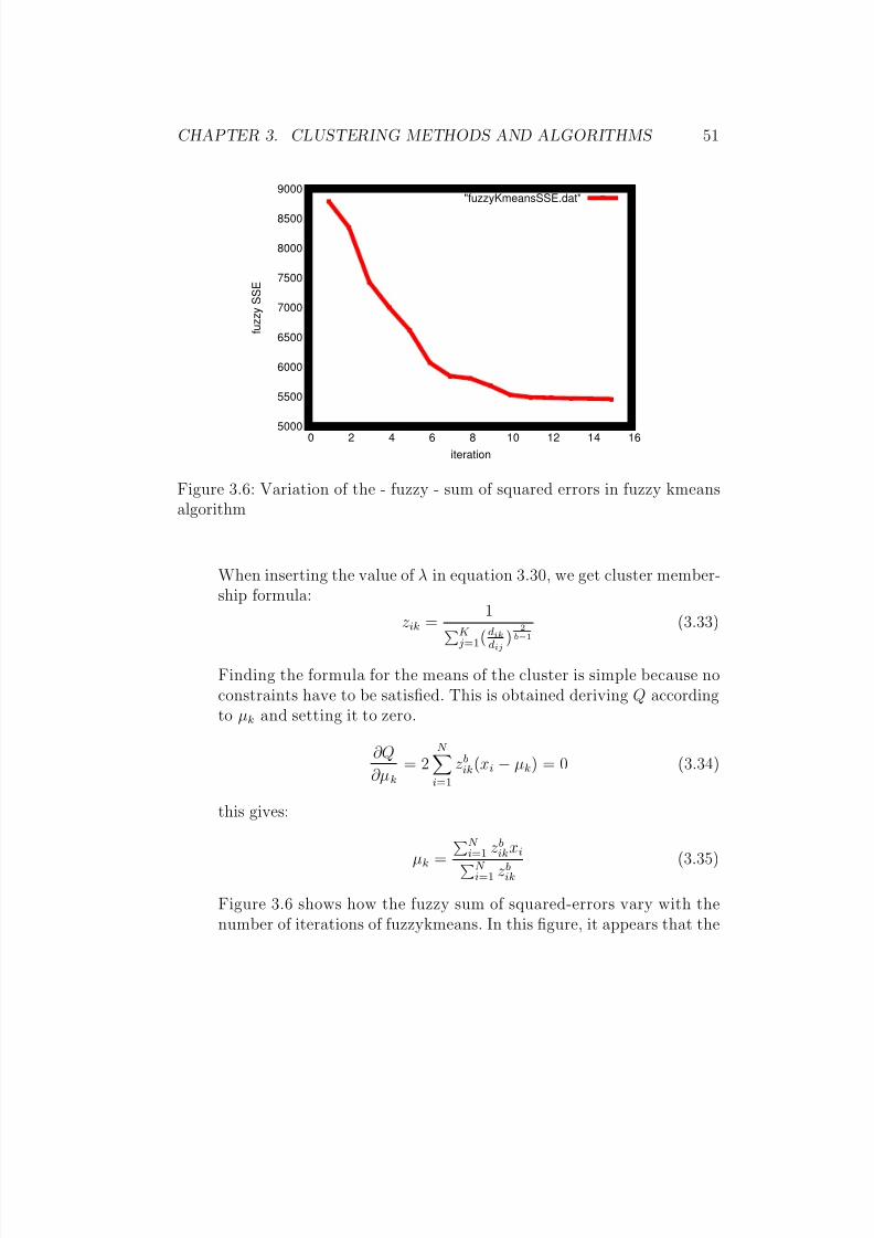
8/8/2019 Comp of Clustering Method
http://slidepdf.com/reader/full/comp-of-clustering-method 60/117
CHAPTER 3. CLUSTERING METHODS AND ALGORITHMS 51
5000
5500
6000
6500
7000
7500
8000
8500
9000
0 2 4 6 8 10 12 14 16
f u z z y S S E
iteration
"fuzzyKmeansSSE.dat"
Figure 3.6: Variation of the - fuzzy - sum of squared errors in fuzzy kmeansalgorithm
When inserting the value of λ in equation 3.30, we get cluster member-ship formula:
zik =1K
j=1( dikdij
)2
b−1(3.33)
Finding the formula for the means of the cluster is simple because noconstraints have to be satisfied. This is obtained deriving Q accordingto µk and setting it to zero.
∂Q
∂µk
= 2N
i=1
zbik(xi − µk) = 0 (3.34)
this gives:
µk =
N i=1 zb
ikxiN i=1 zb
ik
(3.35)
Figure 3.6 shows how the fuzzy sum of squared-errors vary with thenumber of iterations of fuzzykmeans. In this figure, it appears that the
8/8/2019 Comp of Clustering Method
http://slidepdf.com/reader/full/comp-of-clustering-method 61/117
CHAPTER 3. CLUSTERING METHODS AND ALGORITHMS 52
fuzzy sum of squared error decreases very slowly after the 11th itera-
tion. That indicates that convergence of the fuzzy kmeans is reachedaround the 11th iteration.
A limitation of the fuzzy kmeans is that it is more computationallyexpensive when compared to the standard kmeans.Fuzzy clustering is appropriate in situation where the clusters overlap.In this thesis, we are looking for partitions of the data set. So ourinterest in fuzzy clustering is limited to studying the effects that fuzzyconcepts have on clustering results. At the end of the clustering pro-cess, a partition -non-overlapping clusters- is returned using a MAP
assignment, for example.
3.3 Discussion of the classical clusteringmethods
The clustering algorithms discussed in the previous sections of thischapter fall into two groups: the traditional ones and the most recentones. The traditional algorithms are HAC, kmeans, EM-based cluster-ing, CEM-based clustering, SOM, fuzzy kmeans and leader clustering.The most recent ones are examples of density-based clustering suchas DBSCAN and DENCLUE and examples of grid-based clusteringsuch as STING. The categorization of each of the clustering algorithmsas instances of a specific clustering method provides a framework forunderstanding and discussing properties of the algorithms. Althoughthese algorithms belong to different methods, some of them can beeasily related. Kmeans is a special case of classification EM-basedclustering which, in turn, is a special case of EM. Kmeans can also beseen as a special case of fuzzy kmeans clustering. A one-dimensionalSOM, in which only the winner node’s weights are updated during the
competitive learning, is equivalent to the online version of the kmeansalgorithm. The difference between online kmeans and kmeans is thatthe former updates the cluster centres as items are assigned to clusters.Only the centre of the cluster to which a new instance is assigned isrecomputed. The latter assigns all the instances to the clusters be-fore re-computing the centres of the clusters. The relation between
8/8/2019 Comp of Clustering Method
http://slidepdf.com/reader/full/comp-of-clustering-method 62/117
CHAPTER 3. CLUSTERING METHODS AND ALGORITHMS 53
those algorithms will be helpful in explaining the performance of the
algorithms.All the discussed clustering algorithms have their strengths and limita-tions. Generally, each of these algorithms will produce a good clusteringresult if the assumptions and ideas the algorithm is based on match thatof the data set. A major difference between these algorithms are theirrunning times. Model-based clustering algorithms, such as EM-basedclustering and CEM-based clustering, and hierarchical clustering arecomputationally expensive. Online clustering is fast and squared-errorclustering has an acceptable running time. So clustering algorithmssuch as EM-based, CEM-based clustering and HAC are impractical for
clustering large data sets. The computationally time of EM-based clus-tering increases drastically with the number of desired clusters. Theexecution time of SOM increases only slightly with the number of clus-ters -the size of the som-grid.
Of the partitioning clustering methods discussed, only the examplesof density based clustering and grid based clustering are useful in thedetection of clusters of arbitrary shapes and sizes. In both approaches,identifying clusters is achieved by merging small dense clusters. Themain difference in these approaches is how they define and identify thesmall clusters. DENCLUE, which is an example of density based clus-
tering, uses density distribution functions and identifies dense regionsby finding the local maxima of the overall density function. DBSCAN,which is another example of a density based clustering algorithm, local-izes points that contain a number of items above a specified threshold.STING, an example of grid based clustering, uses sufficient statisticsabout grid cells for identifying the dense cells. These algorithms are de-signed for spatial databases. They use efficient spatial data structure,such as R* tree, for merging dense clusters. This makes them scalableto large data sets. Hierarchical agglomerative clusters are also con-structed by merging small clusters. But it is impractical to use HAC
for clustering large data sets because HAC does not use an efficientdata structure.In the next section, we will study the issue of combining clusteringmethods. We will specifically study how the merging of small clusterscan be efficiently adapted to the data set at hand.
8/8/2019 Comp of Clustering Method
http://slidepdf.com/reader/full/comp-of-clustering-method 63/117
CHAPTER 3. CLUSTERING METHODS AND ALGORITHMS 54
3.4 Combining clustering methods
Clustering methods can be combined using two main approaches.
1. The first approach combines the clustering results produced bypairs of clustering algorithms. It deduces new partitions of thedata set by studying the agreement in the clustering results pro-duced by different clustering methods. [32] studied various algo-rithms and techniques for studying the agreement in the partitionsprovided by different clustering methods. This approach will notbe considered in this thesis because it is computationally expen-
sive.2. The second approach combines ideas and techniques from different
clustering methods to derive new clustering techniques. The goalis to use different ideas and techniques from different clusteringmethods as building blocks for new clustering techniques to solvethe problem at hand. Two different architectures will be explored.
– The first involves initialising a clustering algorithm with thepartition produced by another clustering algorithm.
– The second clustering architecture consists in two levels. Thefirst level creates a large number of small clusters using one of
the studied clustering algorithms and the second level mergesthe clusters created at the first level. This clustering archi-tecture will be called two-level clustering.
3.4.1 Two-level clustering with kmeans
We use the two-level architecture in order to detect clusters of arbitraryshapes and sizes. Because the distribution of the attacks is skewed,producing high number of small clusters will help us to identify smallsize attack clusters. Large clusters, consisting for example of normaldata, can be constructed by merging small clusters.
In this study, kmeans is used for the creation of the first level clusters.In principle, the choice of clustering algorithm for the creation of theclusters at the first level does not make a significant difference as longas the clusters created are of high purity. Kmeans has been chosen
8/8/2019 Comp of Clustering Method
http://slidepdf.com/reader/full/comp-of-clustering-method 64/117
CHAPTER 3. CLUSTERING METHODS AND ALGORITHMS 55
because it is fast compared to most of the other algorithms, and because
it has some properties that are essential for the success of the proposedmethod. In the rest of this section, the first level clusters will be referredto as basic clusters.
Merging basic clusters degrades the purity of the clustering. Our aim isto merge clusters in such a way that the purity of the clusters degradesas little as possible. As the attack labels are not known during theclustering process, we do not have a way of directly measuring thepurity of the clustering. Other characteristics of the data will be usedto approximate the purity of clusters.
A cluster is said to be 100% pure if it contains attacks of exactly onekind. Merging two 100% pure clusters, that contains the same attacktype, will not degrade the purity of the clustering. It will be assumedthat two basic clusters are of the same type and therefore can be mergedif the following two conditions are satisfied:- the two clusters are close to each other,- the two clusters have approximately the same density.The first of these conditions is based on the assumption that data in-stances of the same attack type are close to each other. The secondcondition is based on the assumption that clusters of the same attacktype have approximately the same density. The density of a cluster is
defined as the average number of items in a specified radius ρ.
Estimation of the density of basic clusters:Because kmeans is used for the creation of basic clusters, a basic clus-ter size can be used as an approximation of the cluster density. Thisis possible because kmeans is based on the implicit assumption thatclusters are spheres of identical radius δ. So by choosing ρ equal to δthe cluster size can be to estimate cluster density.
Proof of the assumption regarding the shape and size of kmeansclusters:The estimate of the density of basic clusters produced by kmeans isbased on our assertion that kmeans assumes that clusters are spheresof the same size. The goal of this section is to prove this assertion.
As we explained earlier, kmeans aims at minimizing the sum of squared-
8/8/2019 Comp of Clustering Method
http://slidepdf.com/reader/full/comp-of-clustering-method 65/117
CHAPTER 3. CLUSTERING METHODS AND ALGORITHMS 56
errors criterion. Let us recall the expression of the sum of squared-errors
of a partition P.SS E (P ) =
K k=1
x∈C k
||x − µk||2, where µk is the center of cluster C k:µk = 1
|C k|
x∈C kx.
The purpose of the proof is to show that the minimization of the SSEis equivalent to the maximization of a special case classification like-lihood criterion. This special case corresponds to the situation wherethe model is a mixture of isotropic gaussians with identical standarddeviation and with identical mixture proportions. In this special caseCEM aims at finding clusters that are spheres of the same sizes. Theexpression of the classification likelihood criterion, shown earlier, is as
follows:κ(Θ|D) =
K k=1
xik∈Ck
log(αk p(xik|µk, σk)), where C k is the kth clus-ter and µk, σk, αk are respectively its mean, standard deviation andmixture proportion.
In the case where the mixture proportions and standard deviations areidentical for all the clusters, we have:αk = 1/K and σk = σ ∀k, 1 ≤ k ≤ K . So,
κ(Θ|D) =
K
k=1
xik∈Ck
log ((1/K ) p(xik
|µk, σ)), (3.36)
Which is equivalent to:
κ(Θ|D) =K
k=1
xik∈Ck
log p(xik|µk, σ) + R, (3.37)
where R is a constant.Using the expression of the isotropic gaussian, that is: p(xik|µk, σ) =
1(√2πσ)d
exp(−xik−µk22σ2 ),
we get:
κ(Θ|D) =K
k=1
xik∈Ck
((−1
2σ2)||xik − µk||2 + d log(
√2πσ) + R (3.38)
µk is the center of the kth because the maximum likelihood estimateof the mean of a cluster is the center of the cluster -as shown in the
8/8/2019 Comp of Clustering Method
http://slidepdf.com/reader/full/comp-of-clustering-method 66/117
CHAPTER 3. CLUSTERING METHODS AND ALGORITHMS 57
formula of the M step of the CEM algorithm. So,
κ(Θ|D) =−1
2σ2SS E (P ) − N d log(
√2πσ) + R (3.39)
where N is the size of the data set D and d is is the dimension of D.This last equation proves that minimizing SSE is equivalent to maxi-mizing the classification likelihood criterion for a mixture of isotropicgaussians with identical mixture proportion and identical standard de-viation.
Merging basic clusters
In order to produce clusters of arbitrary shapes, basic clusters are linkedinstead of being fused. The linking of basic clusters results in multi-centered clusters. The fusion of basic clusters into one center-basedcluster will have produced spherical clusters. The distance between twomulti-centered clusters is defined as the distance between their closestbasic clusters. The distance between two basic clusters is defined asthe euclidean distance between their means. This distance measure hasbeen chosen because its computation is fast.
Selecting an optimal number of basic clusters :
The parameters that influence the quality of clustering with the two-level approach are: the purity of the basic clusters and the numberof times basic clusters are linked. These two conditions are mutuallyantagonistic. A high purity of basic clusters requires a large number of basic clusters. But with a large number of basic clusters a high numberof linking operations are required. We need a mechanism for choosingan optimal number of basic clusters.Figure 3.7 illustrates how the classification accuracy obtained with two-level clustering varies with the number of basic clusters. Figure 3.7shows that the classification accuracy is highest when the number of
basic clusters is 200.In order to choose the appropriate number of basic clusters, we studyhow the SSE is related to the classification accuracy for kmeans clus-tering. This study shows that SSE and classification accuracy vary ina similar way with the number of clusters of kmeans. So we use SSEfor identifying the optimal number of basic clusters. As SSE measures
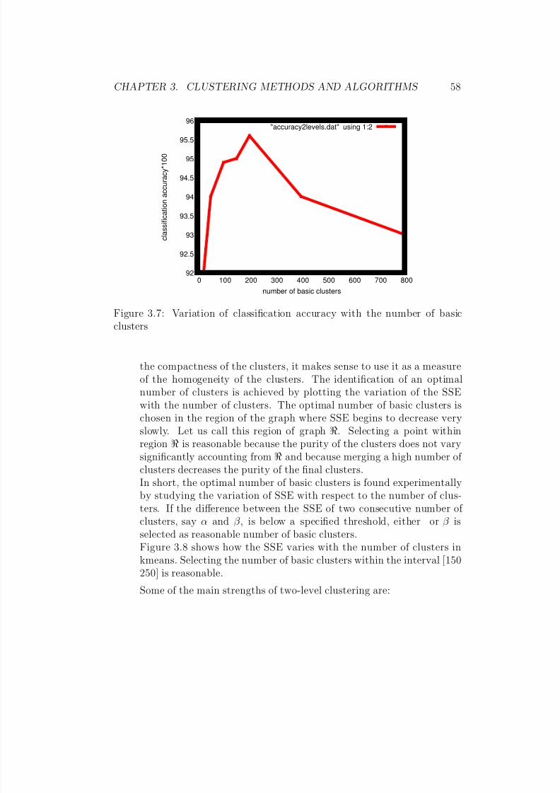
8/8/2019 Comp of Clustering Method
http://slidepdf.com/reader/full/comp-of-clustering-method 67/117
CHAPTER 3. CLUSTERING METHODS AND ALGORITHMS 58
92
92.5
93
93.5
94
94.5
95
95.5
96
0 100 200 300 400 500 600 700 800
c l a s s i f i c a t i o n
a c c u r a c y * 1 0 0
number of basic clusters
"accuracy2levels.dat" using 1:2
Figure 3.7: Variation of classification accuracy with the number of basicclusters
the compactness of the clusters, it makes sense to use it as a measureof the homogeneity of the clusters. The identification of an optimalnumber of clusters is achieved by plotting the variation of the SSEwith the number of clusters. The optimal number of basic clusters ischosen in the region of the graph where SSE begins to decrease veryslowly. Let us call this region of graph . Selecting a point withinregion is reasonable because the purity of the clusters does not varysignificantly accounting from and because merging a high number of clusters decreases the purity of the final clusters.In short, the optimal number of basic clusters is found experimentallyby studying the variation of SSE with respect to the number of clus-ters. If the difference between the SSE of two consecutive number of clusters, say α and β , is below a specified threshold, either or β is
selected as reasonable number of basic clusters.Figure 3.8 shows how the SSE varies with the number of clusters inkmeans. Selecting the number of basic clusters within the interval [150250] is reasonable.
Some of the main strengths of two-level clustering are:
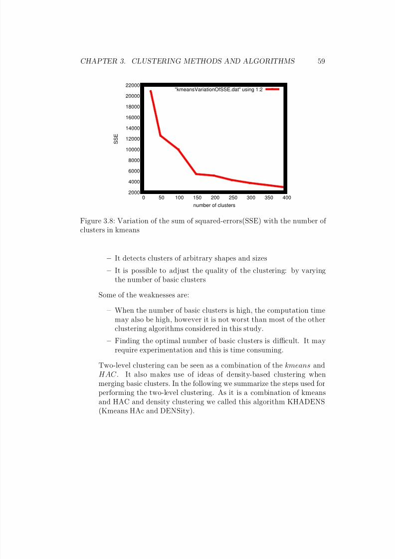
8/8/2019 Comp of Clustering Method
http://slidepdf.com/reader/full/comp-of-clustering-method 68/117
CHAPTER 3. CLUSTERING METHODS AND ALGORITHMS 59
2000
4000
6000
8000
10000
12000
14000
16000
18000
20000
22000
0 50 100 150 200 250 300 350 400
S S E
number of clusters
"kmeansVariationOfSSE.dat" using 1:2
Figure 3.8: Variation of the sum of squared-errors(SSE) with the number of clusters in kmeans
– It detects clusters of arbitrary shapes and sizes
– It is possible to adjust the quality of the clustering: by varying
the number of basic clusters
Some of the weaknesses are:
– When the number of basic clusters is high, the computation timemay also be high, however it is not worst than most of the otherclustering algorithms considered in this study.
– Finding the optimal number of basic clusters is difficult. It mayrequire experimentation and this is time consuming.
Two-level clustering can be seen as a combination of the kmeans and
HAC . It also makes use of ideas of density-based clustering whenmerging basic clusters. In the following we summarize the steps used forperforming the two-level clustering. As it is a combination of kmeansand HAC and density clustering we called this algorithm KHADENS(Kmeans HAc and DENSity).
8/8/2019 Comp of Clustering Method
http://slidepdf.com/reader/full/comp-of-clustering-method 69/117
CHAPTER 3. CLUSTERING METHODS AND ALGORITHMS 60
1. Initialisation: Specify the number of basic clusters β . This is
done through experimentation. Specify the minimum distanceminDist and the minimum rapport of size minDens which twobasic clusters must have in order to be merged.
2. Creation of the basic clusters: Create β clusters using the kmeansalgorithm
Iteration: Repeat step 3 until no change occur
3. Merging clusters Start with the the basic clusters. For each pairof clusters MC 1 and MC 2, merge them if there is a basic clusterbc1 ∈ M C 1 and basic cluster bc2 ∈ MC 2 such that d(bc1, bc2) ≤
minDist and |bc1
||bc2| ≥ minDens.Another variation of this algorithm has been explored. In this variationthat we call KHAC, the closest clusters are iteratively merged until thedesired number of clusters is reached. The main difference betweenthese two algorithms is that the size of basic clusters is not consideredwhen merging clusters in KHAC.
The running time of KHADENS and KHAC is mainly the time usedfor the creation of the basic clusters. The merging of the basic clustersis fast as it generally involves a small number of clusters.
3.4.2 Initialisation of clustering algorithms withthe results of leader clustering
Leader clustering is very fast and robust to outliers. It can, therefore, beused for the identification of better initial cluster centres to be used ineach of the other algorithms. The procedure for initialising a clusteringalgorithm CA with the leader clustering algorithm is the following: LetK be the number of clusters desired by CA. The leader clustering isused to cluster the data set into M clusters, where M
≥K . Then the
centres of K of the clusters created by the leader algorithm are used asinitial centres for the clustering algorithm CA.
8/8/2019 Comp of Clustering Method
http://slidepdf.com/reader/full/comp-of-clustering-method 70/117
CHAPTER 3. CLUSTERING METHODS AND ALGORITHMS 61
3.5 Summary
In this chapter, different clustering methods have been discussed. Adistinction has been made between clustering methods and clusteringalgorithms. A clustering method defines the general concept and theorythe clustering is based on, while a clustering algorithm is a particularimplementation of a clustering method. Examples of each of the con-sidered clustering methods have been discussed. Most of the classicalclustering algorithms considered in this thesis approach the clusteringproblem as an optimisation problem. They aim at optimising a globalobjective function. They make use of an iterative process to solve the
problem. Another group of algorithms do not approach the clusteringproblem as an optimisation problem. They view clusters as dense re-gions in the data space and identify clusters by merging small units of dense regions. This is the case for density based clustering and gridbased clustering. A clustering architecture inspired by some propertiesof the clustering algorithms using an optimisation approach and theclustering algorithms which constructs clusters by making local deci-sions has been proposed. This architecture takes into consideration thecharacteristics of the data set at hand. The discussed clustering algo-rithms, with the exception of DBSCAN, DENCLUE and STING are
used for our experiments, which are discussed in the next chapter.
8/8/2019 Comp of Clustering Method
http://slidepdf.com/reader/full/comp-of-clustering-method 71/117
Chapter 4
Experiments
This section describes and discusses the design and the execution of the experiments. This discussion is important in order to understandand explain aspects of the experiments that have an impact on theperformance of the clustering algorithms.
– Section 4.1 discusses the design of the experiments.
– Section 4.2 discusses the data set and its feature set.
– Section 4.3 discusses implementation issues.– Section 4.4 summarizes the chapter.
The experiments are conducted on a pentium 4 processor with 1.5GB of memory. The operative system is FREEBSD release 5.4.
4.1 Design of the experiments
The design and the implementation are modular. The programminglanguage used for the implementations of the clustering algorithms andthe experiment is C++. As an example of object oriented programminglanguage, C++ supports modularity. Furthermore C++ is an efficientand flexible programming language. The efficiency is an important is-sue in our experiment because of the large size of the data set. The
62
8/8/2019 Comp of Clustering Method
http://slidepdf.com/reader/full/comp-of-clustering-method 72/117
CHAPTER 4. EXPERIMENTS 63
architecture of the system used for implementing the clustering algo-
rithms and performing the experiments is composed of four modules:the data preparation module, the clustering algorithms module, theexperiment module and the evaluation module.
– Data preparation module: this module puts the data in a formthat is easily used by the clustering algorithms. It transformsnon-numeric feature values into numeric feature values and it nor-malizes the feature values.
– Clustering algorithm module: This module implements the dis-tance measures and the clustering algorithms. Common and im-
portant clustering concepts have been encapsulated into classes sothey can be easily share by the different clustering algorithms.
– Experiment module: This module implements operations relatedto the execution of the experiment. It implements for example theexecution of the ten-fold cross validation. It also implements thedifferent indices to be used for evaluation of the algorithms.
– Evaluation module: On the basis of the evaluation indices com-puted in the experiment module, the evaluation module comparesthe clustering algorithms. It computes the means and standarddeviations of the indices and makes a paired t-test comparison.
4.2 Data set
The performance of clustering algorithms partly depends on the char-acteristics of the data set. This section describes and discusses the dataset selected for the experiments.
4.2.1 Choice of data set
The data set chosen for the experiment is the KDD Cup 99 data set.This data set is available at [16]. The KDD Cup 99 data set is aprocessed version of a data set, developed under the sponsorship of theDefense Advanced Research Projects Agency (DARPA) -of the USA- in1998 and 1999, for the off-line evaluation of intrusion detection systems
8/8/2019 Comp of Clustering Method
http://slidepdf.com/reader/full/comp-of-clustering-method 73/117
CHAPTER 4. EXPERIMENTS 64
(IDS) [17, 41]. Currently the DARPA data set is the most widely used
data set for testing IDS.This DARPA project was prepared and executed by the MassachusettsInstitute of Technology (MIT) Lincoln Laboratory. MIT Lincoln Labsset up an environment on a local area network that simulated a mili-tary network under intensive attacks. The simulated network consistsof hundreds of users on thousands of hosts. Working in a simulatedenvironment made it possible for the experimenters to have completecontrol of the data generation process. The experiment was carriedout over nine weeks and a raw network traffic data, also called rawtcpdump data, was collected during this period.
The raw tcpdump data has then been processed into connection recordsused in the KDD Cup 99 data set. The KDD Cup 99 data set containsa rich variety of computer attacks. The full size of the KDD Cup 99 isabout five million network connection records. Each connection recordis described by 41 features and is labelled either as normal or as aspecific network attack. One of the reasons for choosing this data setis that the data set is standard. This will make it easy to compare theresults of our work with other similar works. Another reason is thatit is difficult to get another data set which contain so rich a variety of attacks as the one used here.
Some criticisms have been made about the generation of the DARPAdata set. One the strongest criticisms was made by J. M cHUGH in[42]. The network traffic generated in the DARPA data set has twocomponents: the background traffic data -which consists of networktraffic data generated during the normal usage of the network- and theattack data. According to M cHUGH, the generation process of thebackground traffic data has not been described explicitly by the exper-imenters. Therefore, there is no direct evidence that the backgroundtraffic matches the normal usage pattern of the network to be simu-lated. He made similar criticisms about the generation of the attack
data. The intensive attacks the network has been submitted to do notreflect a real word attack scenario.
Although some of these criticisms are important and can be useful infuture generation off-line intrusion evaluation data sets, the DARPAdata set has many strengths which still make it the best publicly avail-
8/8/2019 Comp of Clustering Method
http://slidepdf.com/reader/full/comp-of-clustering-method 74/117
CHAPTER 4. EXPERIMENTS 65
able data set for evaluation of intrusion detection systems.
4.2.2 Description of the feature set
The choice of the feature set is crucial for the success of clustering.The goal of this section is to describe the feature set, and its ability todiscriminate normal patterns and attack patterns.
Generally, the construction of efficient features for intrusion detection iseither done manually or by semi-automated process. The manual con-
struction of features uses only security domain knowledge while semi-automated feature construction automates part of the feature construc-tion process. To our knowledge, none of the existing feature construc-tion methods for network attack detection fully automates the featureconstruction process.
Stolfo et. al in [14] used a semi-automated approach to identify use-ful features for discriminating normal patterns from attack patterns.Their approach is based on data mining concepts and techniques likelink analysis and sequence analysis. Link analysis determines the re-lation between fields of a data record; sequence analysis identifies the
sequential pattern between records. Their work has led to the featureset describing the data set used in this thesis.
In the following, we will first describe the feature set, then we will givea brief explanation of the approach used in [14] to derive them andfinally a discussion of the discriminative capability of the feature setwill be presented. A short description of the feature set is available inappendix B.1. The full description can be found in [16, 14].
There are 41 features, which fall into different categories: basic featuresand derived features.
1. The basic features describe single network connections.2. The derived features can be divided into content-based features
and traffic based features.
(a) The content-based features are derived using domain knowl-edge.
8/8/2019 Comp of Clustering Method
http://slidepdf.com/reader/full/comp-of-clustering-method 75/117
CHAPTER 4. EXPERIMENTS 66
(b) And the traffic-based features are obtained by studying the
sequential patterns between the connection records as well asthe correlation between basic features.
In order to construct the feature set, the raw tcpdump data has beenpre-processed into connection records. The basic features are directlyobtained from the connection records. The derived features fall intotwo groups: the content-based features and the traffic based features.Content-based features are used for the description of attacks that areembedded in the data portion of the IP packet. The description of these types of attacks requires some domain knowledge and cannot bedone only on the basis of information available in the packet header.Most of these attacks are R2L and U2R attacks. Traffic based featureshave been computed automatically; they are effective for the detectionof DOS and probe attacks. The different types of attack contained inthe data set are described in appendix C.
In order to derive the traffic features, Stolfo et al. made use of analgorithm that identifies frequent sequential patterns. The algorithmtakes the network connection records, described by the current basicfeatures, as input and computes the frequent sequential patterns. Thefrequent episodes algorithm is executed on two different data sets: anintrusion-free data set and a data set with intrusions. Then these tworesults are compared in order to identify intrusion-patterns.
The derived features are constructed on the basis of patterns that onlyappear in intrusion data records. Therefore, they are able to discrim-inate between normal and intrusion connection records. Although ex-perience shows that the feature set considered here discriminates wellbetween normal and intrusive patterns it has some limitations when itis used for anomaly detection. Because the feature set has been derivedon the basis of intrusions in the training data set, the derived featureset cannot describe attacks not included in the training data set. Thefeature set is, therefore, more suitable for misuse detection than foranomaly detection. Another limitation of the feature set is that it maynot discriminate well between normal data and attacks embedded inthe data portion of the data packet. The reason for this is that thefeature set has been constructed primarily on the basis of information
8/8/2019 Comp of Clustering Method
http://slidepdf.com/reader/full/comp-of-clustering-method 76/117
CHAPTER 4. EXPERIMENTS 67
available in the header of the packet. The content-based features may
not describe correctly attacks embedded in the data portion of the IPpacket. These features have been derived from indices that characterizethe session between two communicating hosts. These indices may notbe sufficient to capture the full nature of an attack embedded in thedata portion.
Scaling and normalization of the feature values
The purpose of scaling the feature values is to avoid a situation wherefeatures with large and infrequent values dominate the small and fre-
quent values during the computation of distance. Normalization scalesall the feature values in the range [0 1]. Some examples of scalingschemes are the linear scale, logarithmic scale, and scaling using themean and standard deviation of the feature.The linear scale of feature value x of feature nr. j is:Norm(x) =
x−minjminj−maxj , where min j and max j are respectively the min-
imum and the maximum value of feature j.The logarithmic scale is NormL(x) = Norm(log(x) + 1).And the third scaling scheme, based on the mean and standard devia-tion of the feature nr.j, is defined as: NormD(x) = x−meanj
standard deviationj
The advantage of the linear scale compared to the other two scalingschemes is its simplicity. Furthermore, the linear scale normalizes thefeature values. For these reasons, the linear scale has been used forscaling the feature values.
Handling categorial feature values
All the clustering algorithms considered in this thesis are appropriatefor numerical feature values. As the feature set of the KDD Cup 99
data set is a mixture of continuous and categorical values, we needa mechanism for converting the categorical feature values to numericvalues. Converting from one feature type to another must be done withcare because it may result in the loss of information about the data.This loss of information may affect the discriminative capacity of theresulting feature set.
8/8/2019 Comp of Clustering Method
http://slidepdf.com/reader/full/comp-of-clustering-method 77/117
CHAPTER 4. EXPERIMENTS 68
One way of quantifying categorical feature value is by replacing it by
its frequency. For example, if we consider feature that describes thetransport protocol used for communication, two of its possible valuesare: TCP and UDP. The categorical feature value TCP is converted to0.6 if 60% of the connection records use the TCP protocol.
This conversion scheme has been used earlier in the implementation of CLAD [30]- which is a cluster-based anomaly detection system. It isreasonable to use frequency for quantifying categorical feature valuesbecause values that appear more frequently are less likely to be anoma-lous. The frequency can help us to separate normal connection recordsfrom attack connection records.
Another method for encoding categorical feature values is, the so-called1 to N encoding scheme. In this scheme, each categorical feature is ex-tended to N features where N is the number of different values thisfeature can take. The value of 1 (or 1/N in the normalized form) is setin the columns corresponding to that feature in the extended featurespace, the other columns of that feature in the extended feature spaceare set to 0 to mark the absence of that category.One of the problems with this encoding scheme is that it increases thedimension of the data space. How serious this problem is, depends onthe number of categorical features and on the number of different val-
ues each of them can take.Once the categorical feature values have been converted to numericalvalues and the feature values have been normalized, euclidean distanceis used as the similarity measure between instances.
Usage of the data set
This section describes how the data set is used for the experiments.A 10% version of the KDD Cup data set is also available at [16]. Weuse the 10% version of the KDD Cup data set. The 10% version of the
KDD Cup data set contains the same attack labels as the full version.It has been constructed by selecting, from the original data set, 10% of each of the most frequent attack categories and by keeping the smallerattack categories unchanged. The advantage of using this version of thedata set is that the data set is smaller and therefore faster to process.Working with the original data set would have made the execution of
8/8/2019 Comp of Clustering Method
http://slidepdf.com/reader/full/comp-of-clustering-method 78/117
CHAPTER 4. EXPERIMENTS 69
the experiment impossible on the computation resource at our disposal.
About eighty percent of the data are attacks. Most of these attacksare DOS attacks: neptune and smurf. A large percentage of this dataconsists of duplicates. In order to reduce the size of the data set, weselect only a low percentage of the smurf data and the neptune dataset. This new distribution of attack and normal labels is closer to areal life scenario. Most researches in unsupervised anomaly detectionmake some assumptions about the data set. Without such assumptionsthe task of unsupervised anomaly detection is not possible. The subsetselected for the experiments consists of 10% attacks and 90% normal
data. Table 4.1 shows the distribution of attack categories for this dataset.For each of the 10 phases in the ten-fold cross validation, each clusteringalgorithm is run 3 times. We proceed in this way because most of the algorithms are randomly initialised and the result of clustering isdependent on the initial values. As mentioned above, the instancesof the data set are labelled: either as normal or as a specific attackcategory. The labels are not used during clustering, they are only usedduring the evaluation of the clustering algorithms.
4.3 Implementation issues
The implementations of the clustering algorithms have been kept sim-ple. The implementation has been kept simple because we have focusedon highlighting the basic ideas in each of the clustering algorithms. Wehave avoided optimisation techniques that could possibly influence theclustering result.
In the implementation of two-level clustering, no significant differencehas been observed between linking successively the two closest clusters
until the desired number of clusters is reached (KHAC) and the linkingapproach just described in KHADENS. So for simplicity, KHAC hasbeen used our experiments. One possible reason for why the two merg-ing strategies produce similar result may be that the closest clustershave almost similar size.
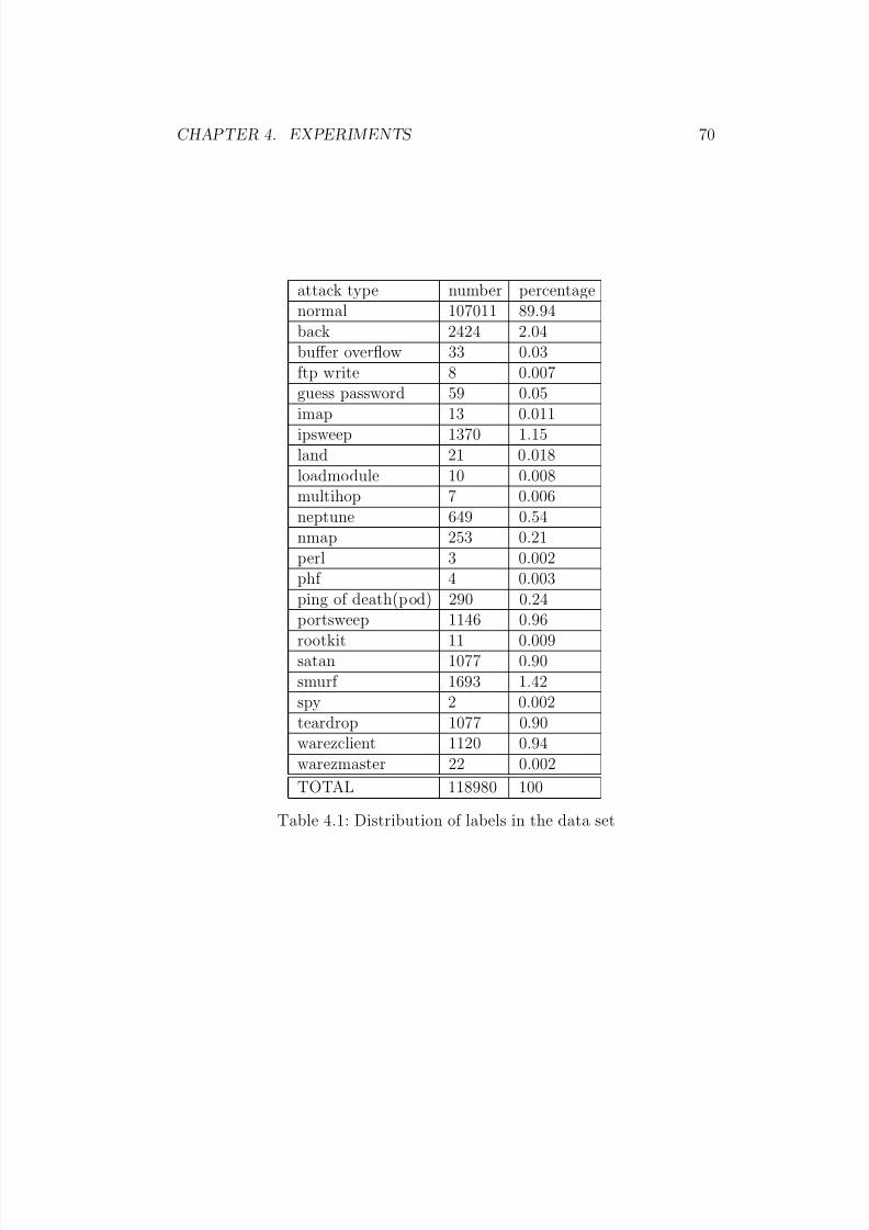
8/8/2019 Comp of Clustering Method
http://slidepdf.com/reader/full/comp-of-clustering-method 79/117
CHAPTER 4. EXPERIMENTS 70
attack type number percentagenormal 107011 89.94back 2424 2.04buffer overflow 33 0.03ftp write 8 0.007guess password 59 0.05
imap 13 0.011ipsweep 1370 1.15land 21 0.018loadmodule 10 0.008multihop 7 0.006neptune 649 0.54nmap 253 0.21perl 3 0.002phf 4 0.003ping of death(pod) 290 0.24
portsweep 1146 0.96rootkit 11 0.009satan 1077 0.90smurf 1693 1.42spy 2 0.002teardrop 1077 0.90warezclient 1120 0.94warezmaster 22 0.002
TOTAL 118980 100
Table 4.1: Distribution of labels in the data set
8/8/2019 Comp of Clustering Method
http://slidepdf.com/reader/full/comp-of-clustering-method 80/117
CHAPTER 4. EXPERIMENTS 71
For each of the clustering algorithms, various tests have been performed
in order to select the best parameter values. The experiments have beenperformed with the best parameter values identified.
4.4 Summary
This chapter has covered the design and execution of our experiments.Special attention has been paid to the data set and feature set used.
– The data set used is a slightly modified version of the KDD data
set. The feature values have been scaled and normalized using alinear scale. The categorical feature values have been transformedto numeric values using a frequency encoding.
– For each of the clustering algorithms, different tests have beenperformed in order to choose the best set of parameters
– The limitation of the feature set for unsupervised anomaly detec-tion has been discussed: Some of these limitations are: Firstly,the algorithm used for the construction of the features relies onthe existence of an attack-free data set. But the fact that it isdifficult to obtain attack-free data set is the main motivation for
performing unsupervised anomaly detection. So for the purposeof unsupervised anomaly detection we need some other methodto compute the feature set. Secondly, for the purpose of anomalydetection, it is the normal traffic patterns we want to describe andnot the attacks, so it is appropriate for us to construct featuresthat describe the normal patterns and not the attacks.
In the next chapter, we evaluate the clustering algorithms.
8/8/2019 Comp of Clustering Method
http://slidepdf.com/reader/full/comp-of-clustering-method 81/117
Chapter 5
Evaluation of clustering
methods
In this chapter the studied clustering algorithms are compared experi-mentally.
– Section 5.1 describes the evaluation methodology used.
– Section 5.2 discusses the evaluation measures.
– Section 5.3 discusses the usage of the k-fold cross validation method.– Section 5.4 presents and analyses the results of the experiments.
– Section 5.5 summarizes the chapter
5.1 Evaluation methodology
The clustering algorithms are evaluated on the basis of external in-dices. External evaluation is possible because data labels are available.Because the considered clustering algorithms are instances of different
clustering methods, external evaluation is the correct method for evalu-ating the algorithms. Evaluating the algorithms on the basis of internalindices, such as the sum of squared-errors, is not appropriate. This isbecause internal indices are generally based on assumptions about theclustering methods used or about the data set. For example, usingthe sum of squared-errors as a measure of compactness and evaluating
72
8/8/2019 Comp of Clustering Method
http://slidepdf.com/reader/full/comp-of-clustering-method 82/117
CHAPTER 5. EVALUATION OF CLUSTERING METHODS 73
the clustering algorithms using it will provide favorable conditions for
squared-errors clustering algorithms such as kmeans.The methodology used for comparing the clustering algorithms is de-scribed below.
We use a ten-fold cross validation. Different experiments in clusterliterature, such as [36], have shown that ten fold is appropriate whenperforming k-fold cross validation. The clusters produced during thetraining phase are used as a classifier and used for the classificationof the test data. The same assignment method and measure used forassigning instances to clusters during training is used for assignmentduring the test. The idea in using cross validation is to measure thegenerality of the clusters produced during the training phase. The k-fold cross validation method is described in the next section. As allof the studied clustering algorithms are dependent on the initialisa-tion values, for each pair of training and test data set of the ten-foldcross validation, the clustering algorithms are run three times. Run-ning the experiments will produce 30 values for each of the evaluationindices and for each of the clustering algorithms. Then for each of theclustering algorithms, the average of the 30 indices and the standarddeviation are computed. A paired t-test is used to compare each pairof clustering algorithms. The paired t-test is used to estimate the sta-
tistical significance of the difference in performance for each pair of algorithms. In order to evaluate the performance of each of the stud-ied clustering algorithms individually, each of them is compared to theresult of a random clustering of the data set. The random clustering isdone by assigning instances to clusters randomly.The experiments are run for two different number of clusters: 23 and49. 23 is the number of categories in the data set. We choose 49 arbi-trary in order to study how the algorithm perform with another numberof clusters.
5.2 Evaluation measures
This section discusses the choice of evaluation measures.
8/8/2019 Comp of Clustering Method
http://slidepdf.com/reader/full/comp-of-clustering-method 83/117
CHAPTER 5. EVALUATION OF CLUSTERING METHODS 74
5.2.1 Evaluation measure requirements
The goal in clustering network traffic data for anomaly detection is tocreate clusters that ideally consist in a single category. The categoryis either a specific attack such as smurf or normal.So the different types of attack/normal category identified by a cluster-ing algorithm are a good indication of how well the algorithm performthis task. We do not expect the clustering algorithms to produce clus-ters that are 100% pure. So the attack category of a cluster is definedto be the label of which there are most of in the cluster. The percent-age represented by the majority of attack labels in a cluster is another
indication of how pure that cluster is.It is also useful to measure whether a cluster contain few attack cate-gories or several attack categories.These requirements lead to the choice of three evaluation measures thatwill be studied in the next section. Each of these evaluation measurescovers one of the requirements. The first one is the number of dif-ferent categories: it counts the different number of attack or normalcategories found by the clustering algorithms. The second is the clas-sification accuracy: it computes the proportion of label of which thereis most of in the cluster. And the third measure is the cluster entropy,which estimates the homogeneity of the clusters.
5.2.2 Choice of evaluation measures
Some of the classical external validation measure found in the litera-ture [23] are the Jacard, Hubert, Rand and Corrected Rand indices.But these measures do not match our requirement that they shouldmeasure the purity of clusters. The measures used in this thesis are:count of cluster categories, classification accuracy and cluster entropy.The count of cluster categories is the number of different cluster cate-
gories found by the clustering algorithm. The category of a cluster isdefined as the label of which there are most of in the cluster.The classification accuracy of a cluster is defined as the proportion rep-resented by the label that is in majority in this cluster. The overallclassification accuracy of the clustering is defined as the weighted meanof the classification accuracy of the clusters produced by this cluster-
8/8/2019 Comp of Clustering Method
http://slidepdf.com/reader/full/comp-of-clustering-method 84/117
CHAPTER 5. EVALUATION OF CLUSTERING METHODS 75
ing.
The cluster entropy has been introduced in [37]. This measure capturesthe homogeneity of clusters. Clusters which contain data from differentattack classes have a higher value. And the clusters, which contain onlyfew attack classes, have low entropy- close to zero. The overall clusterentropy is the weighted mean of the cluster entropies.
Classification accuracy
The classification accuracy of a cluster is the proportion of label most
often found in that cluster. That is
clusterAccuracy =(Size of majority label)
Size of cluster. (5.1)
And the overall classification accuracy of the clustering is the weightedmean of the classification accuracy of the clusters. The weight of acluster is its size divided by the total number of instances.
Cluster entropy
The entropy of the cluster level captures the homogeneity of the clus-ter. The entropy of a cluster is defined as:E clusteri = − j( N ji
ni)log( N ji
ni)
where ni is the size of the ite cluster and N ji is the number of instancesof cluster i which belongs to the class label j.And the cluster entropy is the weighted sum of the cluster entropies:E cluster =
i
niN
E clusteri
where N is the total size of the data set and ni is the number of in-stances in cluster i.
The cluster entropy is lowest when the clusters consists of a single datatypes and it is highest when the proportion of each of data category inthe clusters is the same.
8/8/2019 Comp of Clustering Method
http://slidepdf.com/reader/full/comp-of-clustering-method 85/117
CHAPTER 5. EVALUATION OF CLUSTERING METHODS 76
5.3 k-fold cross validation
K-fold cross validation is used in classification to evaluate the accuracyof classifiers. It consists in randomly dividing the data set in k disjointsubsets of approximately equal size. The classifier is trained and testedk times. Each training uses k-1 subsets and the subset left out is usedfor testing. K-fold cross validation can be adapted to clustering.As with classification, the system is trained and tested k times. Thetraining consists in clustering k-1 of the subsets. The subset left outis used for the test. The test is done by assigning instances of thetest data set to the clusters produced during training. The same as-
signment method and measure used for assigning instances to clustersduring training is also used for assignment during testing. During theassignment in the test phase, the characteristics of the clusters are notupdated. For example, the means of the clusters are not recomputed.So the performance of a clustering indicates how well the algorithmperformed during the training and the test phases.Using an independent test data set makes it possible to evaluate therobustness and the generality of the clusters produced by the clusteringalgorithms. After all, the goal of the off-line clustering we perform is tocreate clusters that will be used for performing a classification of new
data. Therefore it is important that the clustering algorithms are ableto classify correctly an independent data set.
5.4 Discussion and analysis of the exper-iment results
This section analyses the results of the experiments.
5.4.1 Results of the experiments
Figures 5.1, 5.2, 5.3, 5.4, 5.5 and 5.6, located from page 77 to page85, show the experiment result. The data used for the generation of
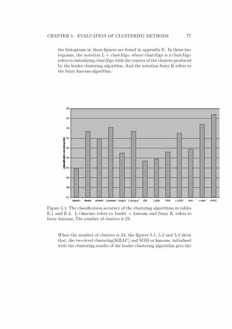
8/8/2019 Comp of Clustering Method
http://slidepdf.com/reader/full/comp-of-clustering-method 86/117
CHAPTER 5. EVALUATION OF CLUSTERING METHODS 77
the histograms in these figures are found in appendix E. In these his-
tograms, the notation L + clustAlgo, where clustAlgo is a clustAlgorefers to initializing clustAlgo with the centres of the clusters producedby the leader clustering algorithm. And the notation fuzzy K refers tothe fuzzy kmeans algorithm.
Figure 5.1: The classification accuracy of the clustering algorithms in tablesE.1 and E.2. L+kmeans refers to leader + kmeans and fuzzy K refers to
fuzzy kmeans. The number of clusters is 23.
When the number of clusters is 23, the figures 5.1, 5.3 and 5.2 showthat, the two-level clustering(KHAC) and SOM or kmeans, initialisedwith the clustering results of the leader clustering algorithm give the
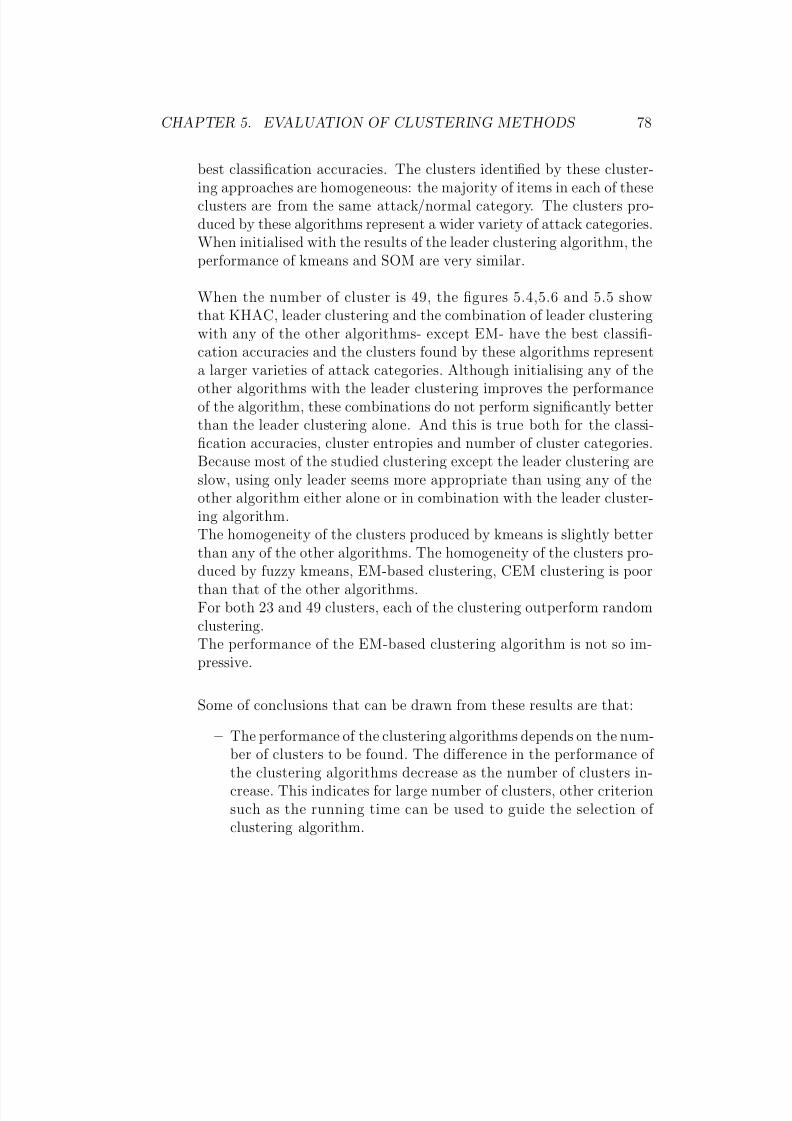
8/8/2019 Comp of Clustering Method
http://slidepdf.com/reader/full/comp-of-clustering-method 87/117
CHAPTER 5. EVALUATION OF CLUSTERING METHODS 78
best classification accuracies. The clusters identified by these cluster-
ing approaches are homogeneous: the majority of items in each of theseclusters are from the same attack/normal category. The clusters pro-duced by these algorithms represent a wider variety of attack categories.When initialised with the results of the leader clustering algorithm, theperformance of kmeans and SOM are very similar.
When the number of cluster is 49, the figures 5.4,5.6 and 5.5 showthat KHAC, leader clustering and the combination of leader clusteringwith any of the other algorithms- except EM- have the best classifi-cation accuracies and the clusters found by these algorithms represent
a larger varieties of attack categories. Although initialising any of theother algorithms with the leader clustering improves the performanceof the algorithm, these combinations do not perform significantly betterthan the leader clustering alone. And this is true both for the classi-fication accuracies, cluster entropies and number of cluster categories.Because most of the studied clustering except the leader clustering areslow, using only leader seems more appropriate than using any of theother algorithm either alone or in combination with the leader cluster-ing algorithm.The homogeneity of the clusters produced by kmeans is slightly betterthan any of the other algorithms. The homogeneity of the clusters pro-duced by fuzzy kmeans, EM-based clustering, CEM clustering is poorthan that of the other algorithms.For both 23 and 49 clusters, each of the clustering outperform randomclustering.The performance of the EM-based clustering algorithm is not so im-pressive.
Some of conclusions that can be drawn from these results are that:
– The performance of the clustering algorithms depends on the num-
ber of clusters to be found. The difference in the performance of the clustering algorithms decrease as the number of clusters in-crease. This indicates for large number of clusters, other criterionsuch as the running time can be used to guide the selection of clustering algorithm.
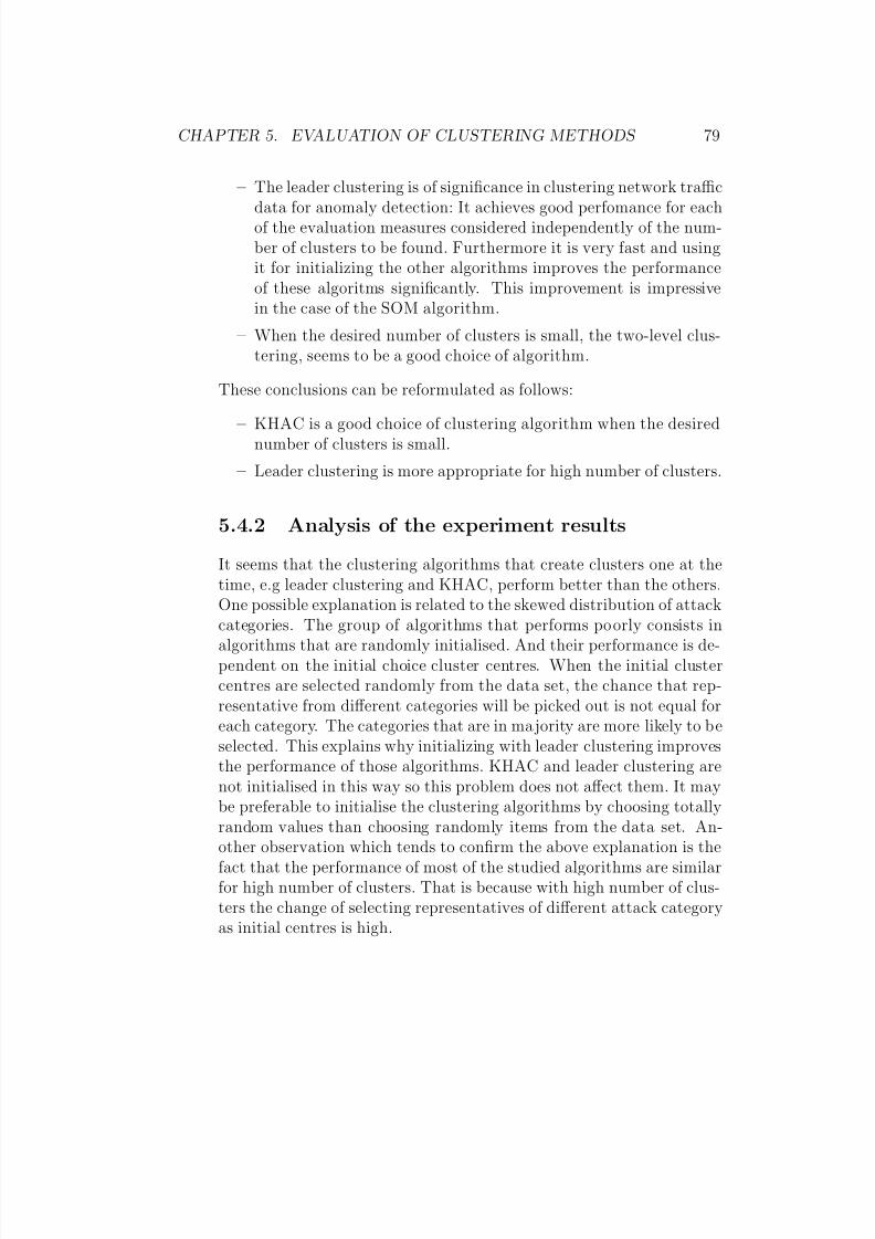
8/8/2019 Comp of Clustering Method
http://slidepdf.com/reader/full/comp-of-clustering-method 88/117
CHAPTER 5. EVALUATION OF CLUSTERING METHODS 79
– The leader clustering is of significance in clustering network traffic
data for anomaly detection: It achieves good perfomance for eachof the evaluation measures considered independently of the num-ber of clusters to be found. Furthermore it is very fast and usingit for initializing the other algorithms improves the performanceof these algoritms significantly. This improvement is impressivein the case of the SOM algorithm.
– When the desired number of clusters is small, the two-level clus-tering, seems to be a good choice of algorithm.
These conclusions can be reformulated as follows:
– KHAC is a good choice of clustering algorithm when the desirednumber of clusters is small.
– Leader clustering is more appropriate for high number of clusters.
5.4.2 Analysis of the experiment results
It seems that the clustering algorithms that create clusters one at thetime, e.g leader clustering and KHAC, perform better than the others.One possible explanation is related to the skewed distribution of attack
categories. The group of algorithms that performs poorly consists inalgorithms that are randomly initialised. And their performance is de-pendent on the initial choice cluster centres. When the initial clustercentres are selected randomly from the data set, the chance that rep-resentative from different categories will be picked out is not equal foreach category. The categories that are in majority are more likely to beselected. This explains why initializing with leader clustering improvesthe performance of those algorithms. KHAC and leader clustering arenot initialised in this way so this problem does not affect them. It maybe preferable to initialise the clustering algorithms by choosing totally
random values than choosing randomly items from the data set. An-other observation which tends to confirm the above explanation is thefact that the performance of most of the studied algorithms are similarfor high number of clusters. That is because with high number of clus-ters the change of selecting representatives of different attack categoryas initial centres is high.
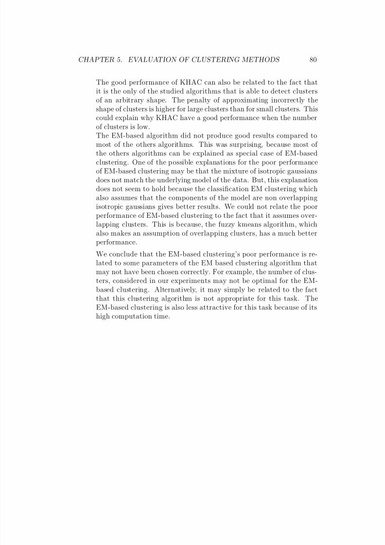
8/8/2019 Comp of Clustering Method
http://slidepdf.com/reader/full/comp-of-clustering-method 89/117
CHAPTER 5. EVALUATION OF CLUSTERING METHODS 80
The good performance of KHAC can also be related to the fact that
it is the only of the studied algorithms that is able to detect clustersof an arbitrary shape. The penalty of approximating incorrectly theshape of clusters is higher for large clusters than for small clusters. Thiscould explain why KHAC have a good performance when the numberof clusters is low.The EM-based algorithm did not produce good results compared tomost of the others algorithms. This was surprising, because most of the others algorithms can be explained as special case of EM-basedclustering. One of the possible explanations for the poor performanceof EM-based clustering may be that the mixture of isotropic gaussians
does not match the underlying model of the data. But, this explanationdoes not seem to hold because the classification EM clustering whichalso assumes that the components of the model are non overlappingisotropic gaussians gives better results. We could not relate the poorperformance of EM-based clustering to the fact that it assumes over-lapping clusters. This is because, the fuzzy kmeans algorithm, whichalso makes an assumption of overlapping clusters, has a much betterperformance.
We conclude that the EM-based clustering’s poor performance is re-lated to some parameters of the EM based clustering algorithm that
may not have been chosen correctly. For example, the number of clus-ters, considered in our experiments may not be optimal for the EM-based clustering. Alternatively, it may simply be related to the factthat this clustering algorithm is not appropriate for this task. TheEM-based clustering is also less attractive for this task because of itshigh computation time.
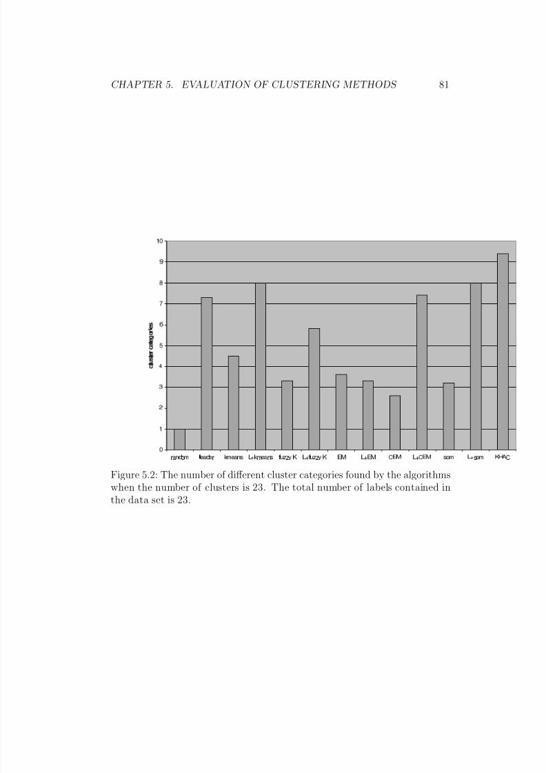
8/8/2019 Comp of Clustering Method
http://slidepdf.com/reader/full/comp-of-clustering-method 90/117
CHAPTER 5. EVALUATION OF CLUSTERING METHODS 81
Figure 5.2: The number of different cluster categories found by the algorithmswhen the number of clusters is 23. The total number of labels contained inthe data set is 23.
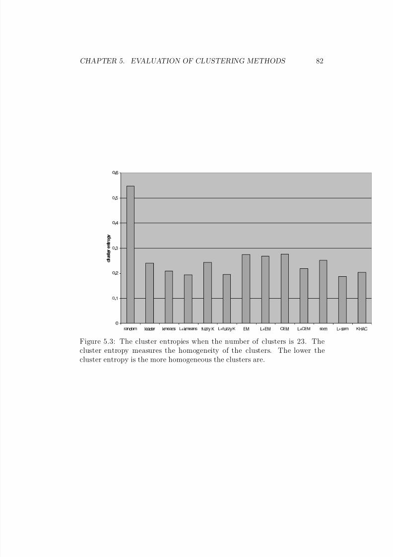
8/8/2019 Comp of Clustering Method
http://slidepdf.com/reader/full/comp-of-clustering-method 91/117
CHAPTER 5. EVALUATION OF CLUSTERING METHODS 82
Figure 5.3: The cluster entropies when the number of clusters is 23. Thecluster entropy measures the homogeneity of the clusters. The lower thecluster entropy is the more homogeneous the clusters are.
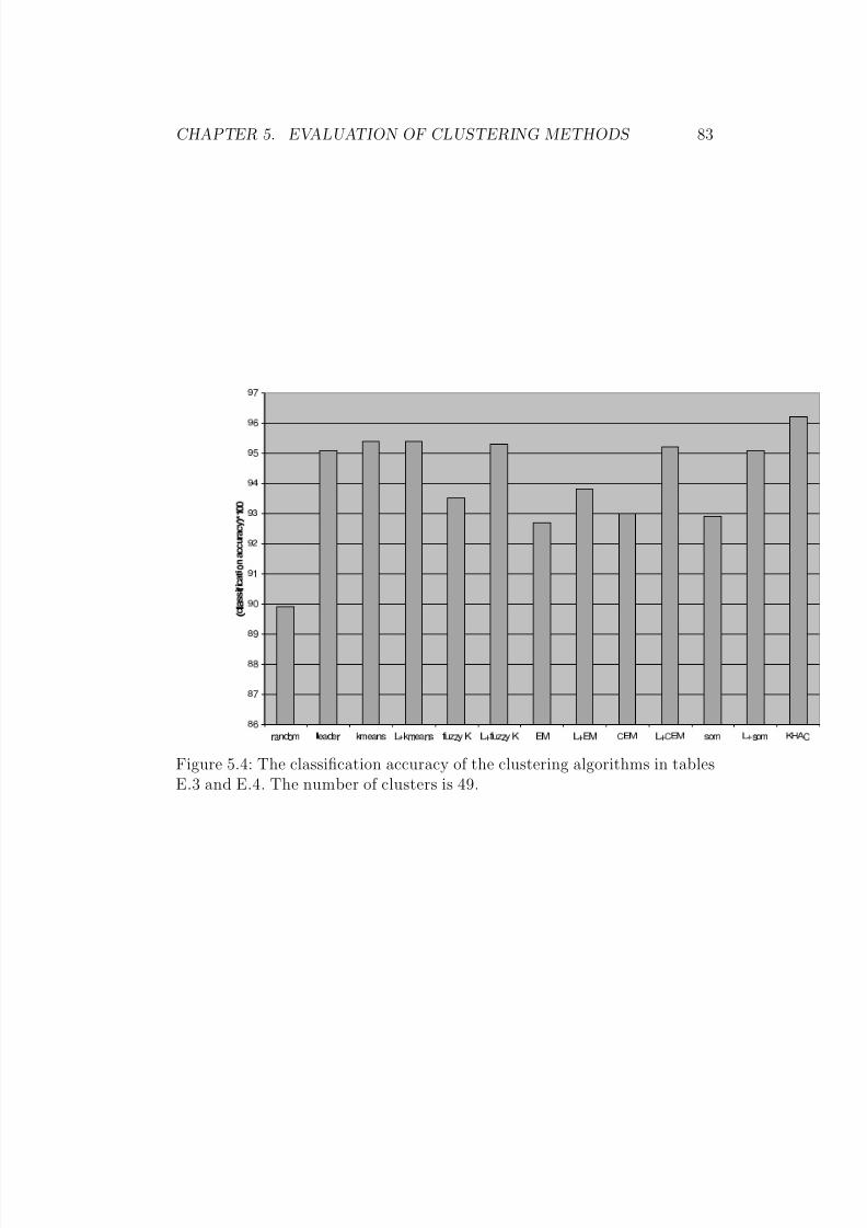
8/8/2019 Comp of Clustering Method
http://slidepdf.com/reader/full/comp-of-clustering-method 92/117
CHAPTER 5. EVALUATION OF CLUSTERING METHODS 83
Figure 5.4: The classification accuracy of the clustering algorithms in tablesE.3 and E.4. The number of clusters is 49.
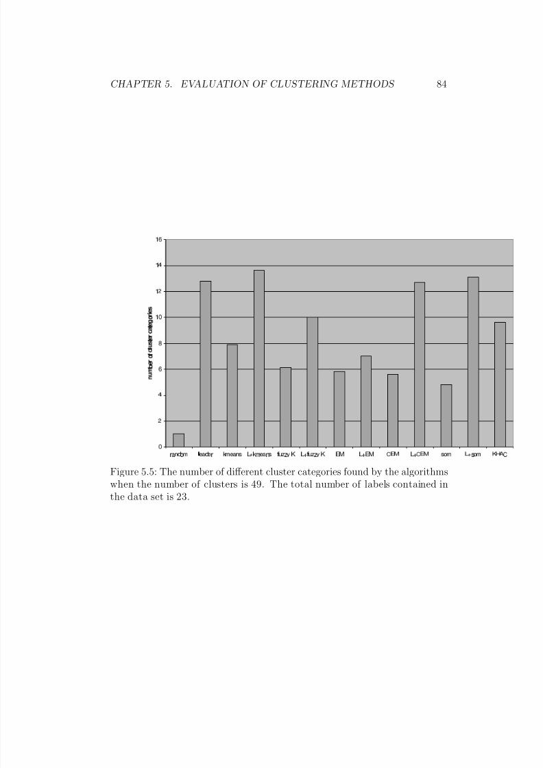
8/8/2019 Comp of Clustering Method
http://slidepdf.com/reader/full/comp-of-clustering-method 93/117
CHAPTER 5. EVALUATION OF CLUSTERING METHODS 84
Figure 5.5: The number of different cluster categories found by the algorithmswhen the number of clusters is 49. The total number of labels contained inthe data set is 23.
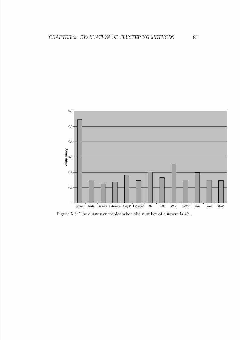
8/8/2019 Comp of Clustering Method
http://slidepdf.com/reader/full/comp-of-clustering-method 94/117
CHAPTER 5. EVALUATION OF CLUSTERING METHODS 85
Figure 5.6: The cluster entropies when the number of clusters is 49.
8/8/2019 Comp of Clustering Method
http://slidepdf.com/reader/full/comp-of-clustering-method 95/117
Chapter 6
Conclusion
6.1 Resume
In this thesis, we have:
– discussed issues of network security and in particular issues con-cerning unsupervised anomaly detection. We have discussed howclustering can be used to solve this problem.
– discussed the clustering problem and the most common cluster-ing methods. Examples of clustering algorithms have also beendiscussed
– implemented and compared classical clustering methods. Theclassical clustering algorithms considered for this study are: stan-dard kmeans, fuzzy kmeans, Expectation Maximization(EM) basedclustering, Classification Expectation Maximization based cluster-ing, Kohonen self organizing feature maps, leader clustering
– investigated two combinations of clustering methods.
∗ The first one uses the results of the leader clustering algorithmfor the initialization of each of the other studied algorithms.This method improves significantly the performance of thesealgorithms.
∗ The second combination is a technique we have proposed.Essentially, this technique is a combination of Kmeans and
86
8/8/2019 Comp of Clustering Method
http://slidepdf.com/reader/full/comp-of-clustering-method 96/117
CHAPTER 6. CONCLUSION 87
Hierarchical Agglomerative Clustering. We call this combi-
nation KHAC. The purpose of KHAC is to create a largenumber of small clusters using kmeans and then merge thesesmall clusters in a similar fashion to hierarchical agglomer-ative clustering. The advantage of this clustering techniqueis its ability to detect arbitrarily shaped clusters. We foundthat KHAC gives better results compared to most of the otherstudied algorithms. The performance of KHAC is especiallyimpressive for small numbers of final clusters.
On the basis our results, we can say that clustering can be successfullyused for unsupervised anomaly detection. Some of the clustering algo-rithms are more appropriate for this task than others. We investigatedthe potential of the leader clustering algorithm. This algorithm is verysimple and fast and produces good clustering results compared to mostof the other studied algorithms. When leader clustering is used forinitializing the other clustering algorithms, included in this thesis, theclustering results of these algorithms improve significantly.
6.2 Achievements
The main goal of the thesis has been to investigate the efficiency of dif-ferent classical clustering algorithms in clustering network traffic datafor unsupervised anomaly detection. The clusters obtained by cluster-ing the network traffic data set are intended to be used by a securityexpert for manual labelling. A second goal has been to study somepossible ways of combining these algorithms in order to improve theirperformance. We can say that these goals have been achieved. Theresults of our experiments have given us an indication of which cluster-ing algorithms are good for this task and which ones are less suitablefor this task. Furthermore, we have studied ways of combining cluster-
ing ideas in order to efficiently solve the problem. We have found outthat, when the number of clusters is low, KHAC which is a combina-tion of clustering concepts we have proposed, produces better resultsthan most of the other studied algorithms. Our data shows the poten-tial of leader clustering algorithm in performing this task. Clusteringalgorithms similar to leader cluster algorithm have been successfully
8/8/2019 Comp of Clustering Method
http://slidepdf.com/reader/full/comp-of-clustering-method 97/117
CHAPTER 6. CONCLUSION 88
used in some earlier works [6, 30] for clustering network traffic data.
The reasons for using this particular algorithm have not been explic-itly stated in these works. In conclusion for our thesis we can say thatleader clustering is to be preferred, not only because it is fast but alsobecause it perform better than most of the other clustering algorithms.So leader-like clustering algorithms could be investigated further in fu-ture research on unsupervised detection. What make them speciallyattractive is their scalability to a large data set. And KHAC seemsattractive when the number of clusters is low.
6.3 LimitationsOne of the limitations of this thesis is that it has not possible to validatethe conclusions of the experiments against a real life data set. This hasnot been possible because of the difficulties of acquiring such a dataset.
6.4 Future work
This work will serve as a first step in building a complete cluster-basedanomaly detection system.
8/8/2019 Comp of Clustering Method
http://slidepdf.com/reader/full/comp-of-clustering-method 98/117
Bibliography
[1] A comparative Study of Anomaly Detection Schemes
in Network Intrusion Detection, A. Lazarevic, L. Er-toz, V. Kumar, A. Ozgur, J. Srivastava
[2] A.K. Jain, M.N. Murty and P.J Flynn. Data cluster-ing: A Review. ACM Computing Surveys, Vol. 31,No.3, September1999.
[3] Richard O. Duda, Peter E. Hart and David D. Stork. Pattern Classification.John Wiley & sons, second edition, 2001.
[4] Eleazar Eskin. Anomaly Detection over noisy data using learned probabil-ity distribution, located at: http://citeseer.ist.psu.edu/eskin00anomaly.html,2000.
[5] Arthur Dempster, Nan Laird, and Donald Rubin. Maximum likelihood fromincomplete data via the EM algorithm. Journal of the Royal Statistical So-ciety B, 39, 1-38, 1977.
[6] Leonid Portnoy. Intrusion detection with unlabeled data using clustering.located at: http://citeseer.ist.psu.edu/574910.html, 2001
[7] E. Eskin, A. Arnold, M. Prerau, L. Portnoy and S. Stolfo. A geometric Frame-work for Unsupervised Anomaly Detection: Detecting Intrusion in UnlabeledData. available at: http://www.cs.cmu.edu/˜ aarnold/ids/uad-dmsa02.pdf,2002
[8] Dorothy E. Denning, An intrusion detection model, IEEE Transactions onsoftware engineering, vol SE-13, No 2, Februar 1987 pages: 222-232 alsolocated at: http://www.cs.georgetown.edu/ denning/infosec/ids-model.rtf.
[9] S. T. Brugger. Data mining methods for network intrusion detection,University of California, Davis, appeared in ACM and available at:http://www.bruggerink.com/ zow/papers/bruggerdmnidsurvey.pdf, 2004.
89
8/8/2019 Comp of Clustering Method
http://slidepdf.com/reader/full/comp-of-clustering-method 99/117
BIBLIOGRAPHY 90
[10] Recent Advance in Clustering : a brief review, S.B. KoTSIANTIS, P.E. PIN-
TELAS[11] Mining in a data-flow environment: Experience in network intrusion detec-
tion. In proc. 5th ACM SIGKDD Int. Conf. Knowledge Discovery and datamining, 114-124, W. Lee;S. Stolfo, and K. Mok 1999.
[12] J. He, A.H. Tan, C.L. Tan, and S.Y. Sung. On Quantitative Evaluationof Clustering Systems. In W.Wu, H. Xiong and S. Shekhar Clustering andInformation retrieval(pp. 105-133), Kluwer Academic Publishers, 2004.
[13] K. Kendall. A database of Computer Attacks for the Evaluation of IntrusionDetection Systems, Master thesis, Massachusetts Institute of Technology,
1999.[14] W. Lee and S.J. Stolfo, A Framework for constructing features and models for
intrusion detection systems, ACM Transactions on Information and SystemSecurity, Vol.3 No.4, November 2000, pages 227-261.
[15] The internet traffic archive ( 2000): http://ita.ee.lbl.gov
[16] KDD cup 99. Located at: http://kdd.ics.uci.edu/databases/kddcup99/kddcup99.html
[17] DARPA. Located at: http://www.ll.mit.edu/IST/ideval/
[18] Clustering large datasets, D.P. Mercer, october 2003
[19] I. Costa, F. de Carvalho, Maricilio C.P de Souto. Comparative analysis of clustering methods for gene expression time course data,
[20] Boris Mirkin. Mathematical Classification and Clustering, Kluwer AdemicPublishers, 1996.
[21] Robert Rosenthal and Ralph L. Rosnow, Essentials of Behavioral Research,Methods and Data Analysis, second edition, 1991.
[22] Jiawei Han and Micheline Kamber. Data Mining, Concepts and Techniques,Morgan Kaufmann Publishers ,2001.
[23] Anil K. Jain, Richard C. Dubes. Algorithms for clustering data, Prentice
Hall, 1988.[24] Giles Celeux and Gerard Govaert. A classification EM algorithm for cluster-
ing and two stochastic versions, INRIA, 1991.
[25] Stuart J.Russel and Peter Norvig. Artificial Intelligence, a modern approach, second edition , Prentice Hall, 2003.
8/8/2019 Comp of Clustering Method
http://slidepdf.com/reader/full/comp-of-clustering-method 100/117
BIBLIOGRAPHY 91
[26] Thomas P. Minka. Expectation maximization as
lower bound maximization, 1998, tutorial located at:http://research.microsoft.com/˜ minka/papers/em.html
[27] An efficient approach to clustering in large multimedia database with noiseAlexander Hinneburg , Daniel A. Keim American Association for artificialintelligence (www.aaai.org) 1998
[28] STING: A STastiscal Information Grid Approach to Spatial data Mining 1997, Wei Wang, Jiong Yang and Richard Muntz. [In twenty-third Internationalconference on very large data bases pp. 186-195 Athens, Greece. MorganKaufmann ]
[29] Ben Krose and Patrick van der Smagt. Artificial Neural Networks, eightedition november, 1996.
[30] Learning rules and clusters for anomaly detection in network traffic: PhilippK. Chan, Matthew V. Mahoney, and Muhammad H. Arshad. Located at:http://www.cs.fit.edu/ pkc/papers/cyber.pdf, Florida Institute of Technol-ogy and Massachusetts Institute of Technology.
[31] Sushmita Mitra,Tinku ACharya. Data mining, multimedia, soft computingand bioinformatics. Wiley Interscience, 2003.
[32] Ludmila I. Kuncheva. Combining pattern classifiers, methods and algorithms.Wiley Interscience, 2004.
[33] A. Ben-Hur, A. Elisseeff and I. Guiyon. A stability based method for discov-ering structure clustered data In. Proc. Pacific Symposium on Biocomputing,2002,pp. 6-17 ?
[34] Wenke lee, Salvatore J. Stolfo, Kui W. Mok, Mining in a data-flow environ-ment. Experience in network intrusion detection, March 1999.
[35] Comparative analysis of clustering methods for gene expression time coursedata , Costa et.al august 2004
[36] Ron Kohavi. A study of Cross-validation and Bootstrap for Accuracy Estima-tion and Model Selection, International Conference on Artificial Intelligence,1995.
[37] Daniel Boley. Principal direction divisive partitioning. Data Mining andKnowledge Discovery, 2(4) :325-344, 1998,
[38] Michalis Vazirgiannis, Maria Halkidi, Dimitrios Gunopulos. Uncertainty han-dling and quality assessment in data mining, Springer 2003.
8/8/2019 Comp of Clustering Method
http://slidepdf.com/reader/full/comp-of-clustering-method 101/117
BIBLIOGRAPHY 92
[39] Wenke Lee and S. J. Stolfo. Data Mining Approaches for Intrusion Detection,
1998.[40] Stefano Zanero and Sergio M. Savaresi. Unsupervised learning techniques for
an intrusion detection system, ACM March 2004.
[41] R. Lippmann, J.w.Haines, D.J. Fried,J. Korba and K. Das. The 1999 DARPAOff-line Intrusion Detection Evaluation, Lincoln Laboratory MIT, 2000.
[42] John M cHUGH. Testing Intrusion Detection Systems: A Critique of 1998and 1999 DARPA Intrusion Detection System Evaluations as Performed byLincoln Laboratory, ACM Transactions on Information and System Security,Vol.3, No. 4, November 2000 pages 262-294.
[43] E. Eskin,M. Miller,Z. Zhong,G. Yi, W. Lee, and S. Stolfo. Adaptive modelgeneration for intrusion detection systems.
[44] http://www.cert.org/stats/cert stats.html#incidents
[45] https://www.cert.dk/artikler/artikler/CW30122005.shtml
[46] Martin Ester, Hans-Peter Kriegel,Jorg Sander,Xiaowei Xu. A density-basedclustering algorithm for discovering Clusters in Large Spatial databases withnoise. Proceedings of 2nd international Conference on Knowledge Discoveryand Data Mining, 1996.
[47] Teuvo Kohonen. Self-organizing maps, 2nd edition Springer, 1997.
[48] A. Ultsch and C. Vetter. Self-organizing-feature-maps versus sta-tistical clustering methods: A benchmark. University of Marbug.Research Report 0994. located at: http://www.mathematik.uni-marburg.de/d̃atabionics/de//downloads/papers/ultsch94benchmark.pdf,[accessed 15/02/2006]
[49] Ross J. Anderson. Security Engineering: A guide to building dependabledistributed systems. John Wiley & Sons, 2001.
[50] A. Wespi, G. Vigna and L.Deri. Recent Advances in Intrusion Detection.5th International Symposium, Raid 2002 Zurich, Switzerland, October 2002Proceedings. Springer.
[51] D. Gollmann. Computer Security. John Wiley & Sons, 1999.
[52] P. Giudici. Applied Data Mining: Statistical Methods for Business and In-dustry. Wiley,2003.
[53] Bjarne Stroustrup. The C++ programming language, third edition, Addison-Wesley, 1997.

8/8/2019 Comp of Clustering Method
http://slidepdf.com/reader/full/comp-of-clustering-method 102/117
BIBLIOGRAPHY 93
[54] http://www-iepm.slac.stanford.edu/monitoring/passive/tcpdump.html
8/8/2019 Comp of Clustering Method
http://slidepdf.com/reader/full/comp-of-clustering-method 103/117
Appendix A
Definitions
A.1 Acronyms
DOS: Denial of service attacks.OS : Operative systems.IDS: Intrusion detection systems.NIDS: Network intrusion detection systems.pod: Ping of Death.
IP: Internet Protocol.TCP: Transport Control Protocol.UDP: User Datagram Protocol.ICMP: Internet control message protocol.HTTP: hypertexts Transport Protocol.FTP: File Transfer Protocol.
A.2 Definitions
Network TrafficIn this thesis network traffic refers to transfer of IP packets throughnetwork communication channels.
Firewalls
94
8/8/2019 Comp of Clustering Method
http://slidepdf.com/reader/full/comp-of-clustering-method 104/117
APPENDIX A. DEFINITIONS 95
Firewalls are security systems protecting the boundary of an internal
network.
To broadcast a messageTo broadcast a message consists in delivering that message to everyhost on a -given- network.
PingA program that is used to test if a connection can be established to aremote host.
ProtocolA protocol is a specifies how modules running on different hosts shouldcommunicate with each other.
HostA host is a synonym for computer.
CGI scriptsA CGI (common gateway interface) script is a program running on aserver and which can be invoked by a client from the CGI interface.
Client and ServerOn a network, a client is the host that requests service from anotherhost. And the host delivering the service is called the server.
TCP connectionA TCP connection is a sequence of IP packets flowing from the packetsender to the packet receiver under the control of a specific protocol.The duration of the connection is limited in time.
Tcpdump
Is a log obtained by monitoring network traffic. Different tools existfor sniffing network traffic. On such a tool which has been used forcollecting the network traffic data used in this thesis is the programcalled TCPDUMP [54].
Data mining

8/8/2019 Comp of Clustering Method
http://slidepdf.com/reader/full/comp-of-clustering-method 105/117
APPENDIX A. DEFINITIONS 96
Data mining is the process of extracting useful models from large vol-
ume of data.
8/8/2019 Comp of Clustering Method
http://slidepdf.com/reader/full/comp-of-clustering-method 106/117
Appendix B
Feature set
B.1 The feature set of the KDD Cup 99data set
Tables B.1, B.2 and B.3 respectively describe the basic features, thecontent-based features and the traffic-based features of the KDD Cup99 data set.
97
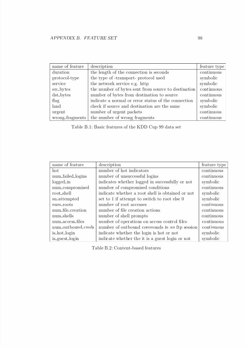
8/8/2019 Comp of Clustering Method
http://slidepdf.com/reader/full/comp-of-clustering-method 107/117
APPENDIX B. FEATURE SET 98
name of feature description feature typeduration the length of the connection is seconds continuousprotocol-type the type of -transport- protocol used symbolicservice the network service e.g. http symbolicsrc bytes the number of bytes sent from source to destination continuousdst bytes number of bytes from destination to source continuousflag indicate a normal or error status of the connection symbolicland check if source and destination are the same symbolicurgent number of urgent packets continuous
wrong fragments the number of wrong fragments continuous
Table B.1: Basic features of the KDD Cup 99 data set
name of feature description feature typehot number of hot indicators continuous
num failed logins number of unsuccessful logins continuouslogged in indicates whether logged in successfully or not symbolicnum compromised number of compromised conditions continuousroot shell indicate whether a root shell is obtained or not symbolicsu attempted set to 1 if attempt to switch to root else 0 symbolicnum roots number of root accesses continuousnum file creation number of file creation actions continuousnum shells number of shell prompts continuousnum access files number of operations on access control files continuousnum outbound cmds number of outbound commands in an ftp session continuous
is hot login indicate whether the login is hot or not symbolicis guest login indicate whether the it is a guest login or not symbolic
Table B.2: Content-based features
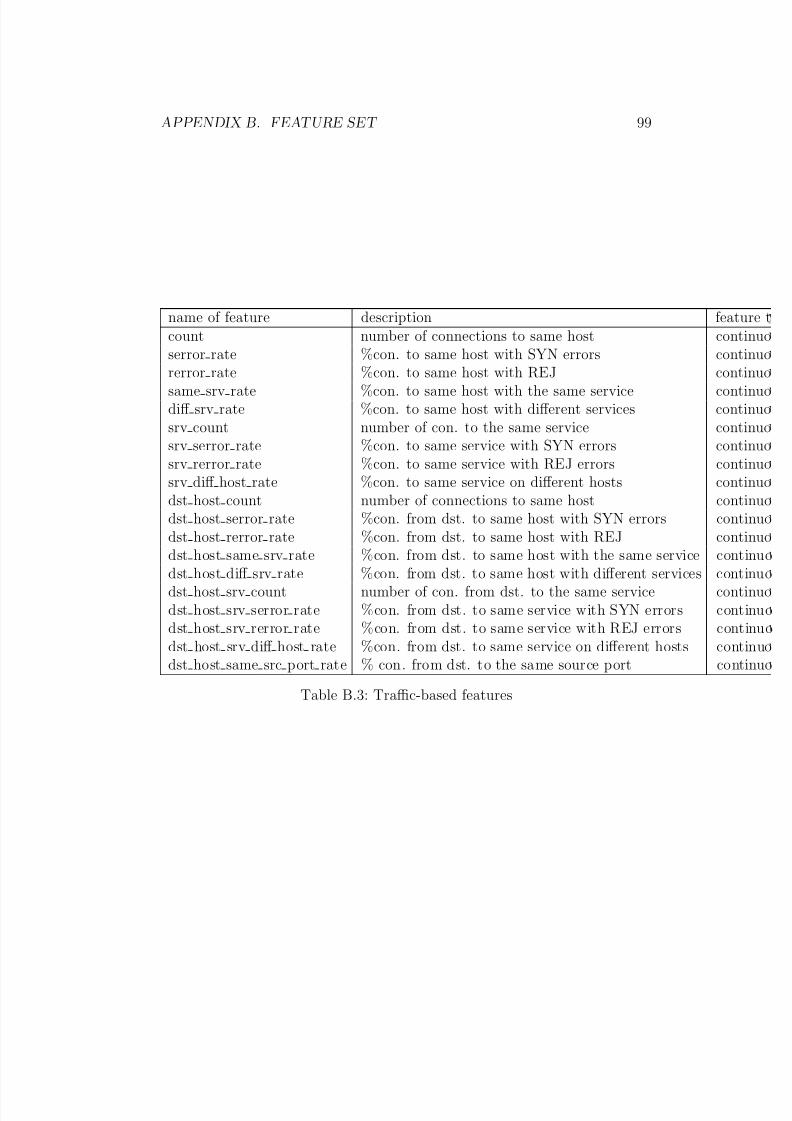
8/8/2019 Comp of Clustering Method
http://slidepdf.com/reader/full/comp-of-clustering-method 108/117
APPENDIX B. FEATURE SET 99
name of feature description feature tcount number of connections to same host continuoserror rate %con. to same host with SYN errors continuo
rerror rate %con. to same host with REJ continuosame srv rate %con. to same host with the same service continuodiff srv rate %con. to same host with different services continuosrv count number of con. to the same service continuosrv serror rate %con. to same service with SYN errors continuosrv rerror rate %con. to same service with REJ errors continuosrv diff host rate %con. to same service on different hosts continuodst host count number of connections to same host continuodst host serror rate %con. from dst. to same host with SYN errors continuodst host rerror rate %con. from dst. to same host with REJ continuo
dst host same srv rate %con. from dst. to same host with the same service continuodst host diff srv rate %con. from dst. to same host with different services continuodst host srv count number of con. from dst. to the same service continuodst host srv serror rate %con. from dst. to same service with SYN errors continuodst host srv rerror rate %con. from dst. to same service with REJ errors continuodst host srv diff host rate %con. from dst. to same service on different hosts continuodst host same src port rate % con. from dst. to the same source port continuo
Table B.3: Traffic-based features
8/8/2019 Comp of Clustering Method
http://slidepdf.com/reader/full/comp-of-clustering-method 109/117
Appendix C
Computer attacks
Here is a list of the computer attacks considered in this thesis:
C.1 Probe attacks
– Ipsweepprobes the network to discover available services on the network.
– Portsweepprobes a host to find available services on that host.
– Nmapis a complete and flexible tool for scanning a network either ran-domly or sequentially.
– Satan
is an administration tool; it gathers information about the net-work. This information can be used by an attacker.
100
8/8/2019 Comp of Clustering Method
http://slidepdf.com/reader/full/comp-of-clustering-method 110/117
APPENDIX C. COMPUTER ATTACKS 101
C.2 Denial of service attacks
– Ping of death (pod) makes the victim host unavailable by sendingit oversized ICMP packets as ping requests.
– Backis a denial of service attack against Apache webservers. The at-tacker sends requests containing many front slashes. The process-ing of which is time consuming.
– Land:Spoofed SYN packet sent to the victim host resulting in that thathost repeatedly synchronizing with itself.
– Smurf A broadcast of ping requests with a spoofed sender address whichresults in that the victim being bombarded with a huge numberof ping responses.
– Neptune:
The attacker half opens a number of TCP connections to the vic-tim host making it impossible for the victim host to accept newTCP connections from other hosts.
– Teardrop:Confuses the victim host by sending it overlapping IP fragments:overlapping IP fragments are incorrectly dealt with by some olderoperating systems.
C.3 User to root attacks
– LoadmoduleThis attack exploits a flaw in how SUNOS 4.1 dynamically loadmodules. This flaw makes it possible for any user of the system
8/8/2019 Comp of Clustering Method
http://slidepdf.com/reader/full/comp-of-clustering-method 111/117
APPENDIX C. COMPUTER ATTACKS 102
to get root privileges.
– Perl:Exploits a bug in some PERL implementations on some earliersystems. This bug consists in these PERL implementations im-properly handling their root privileges. This leads to a situationwhere any user can obtain root privileges.
– Buffer overflowConsists in overflowing input buffers in order to overwrite memorylocations containing security relevant information.
C.4 Remote to local attacks
– ImapImap causes a buffer overflow by exploiting a bug in the authenti-cation procedure of the imap server on some versions of LINUX.The attacker gets root privileges and can execute an arbitrary se-quence of commands.
– Ftp writeThis attack exploits a misconfiguration affecting write privilegesof anonymous accounts on an FTP server.This allows any ftp user to add arbitrary files to the FTP server.
– Phf Is an example of badly written CGI scripts that is distributedwith the apache server. Exploiting this flaw allows the attacker
to execute codes with the http privileges.
– WarezmasterThe warezmaster attack is possible in a situation where write per-missions are improperly assigned on a FTP server.When this is the case, the attacker can upload copies of illegal
8/8/2019 Comp of Clustering Method
http://slidepdf.com/reader/full/comp-of-clustering-method 112/117
APPENDIX C. COMPUTER ATTACKS 103
software that can then be download by other users.
– WarezclientThe Warezclient attack consists in downloading illegal softwarepreviously upload during a warezmaster attack.
C.5 Other attack scenarios
The four categories of attacks described take place usually during a
single session.In most realistic attack scenarios, the attacker performs his attack overa certain period of time in order to minize the chances of detection andin order to perform more precise and successful attacks.These attack scenarios are performed by combining some the basis at-tack categories described.
Here are some of these attacks scenarios:
– Guessing passwords
– Making use of spy programsA spy program monitors the activity on the victim host and makesinformation available to the attacker.
– Making use of rootkitA rootkit is a program that hides the presence of other -malicious-programs or data files. Spyware programs often make use of rootk-its in order to avoid detection by anti-spyware programs.
– Multihop attackThis attack first affects a host on a network and then uses thathost to attack other hosts on the network.
8/8/2019 Comp of Clustering Method
http://slidepdf.com/reader/full/comp-of-clustering-method 113/117
Appendix D
Theorems
D.1 Algorithm: Hill climbing
The hill-climbing algorithm is a local optimisation algorithm.
• Hill climbing algorithm Let g(x) be the gradient of a function f (x).In searching for the maximizer of f (x), the algorithm proceeds as fol-
lows:- It starts with an arbitrary solution s0 ∈ S , where S is the solutionspace.- Then a sequence {st, t ≥ 0} of solutions that approaches the max-imizer of f (x) is constructed. The sequence is defined as: st+1 =αg(xt) + (1 − α)xt, where α > 0.
D.2 Theorem: Jensen’s inequality
Let f be a convex function defined on an interval I .If x1,...,xn ∈ I and α1,...,αn ≥ 0 with
ni=1 = 1,
f (n
i=1
αixi) ≤n
i=1
αif (xi) (D.1)
104

8/8/2019 Comp of Clustering Method
http://slidepdf.com/reader/full/comp-of-clustering-method 114/117
APPENDIX D. THEOREMS 105
D.3 Theorem: The Lagrange method
Let f : Rn → R and g : Rn → R be C 1- that is f and g are derivable andtheir respective derivative are continuous. Let α ∈ Rn such that g(α) = 0(g is the gradient of g). If α is an extremum of f under the constraintg(x1,...,xn) = 0, ∃λ ∈ R such that
f (α) = λg(α) (D.2)

8/8/2019 Comp of Clustering Method
http://slidepdf.com/reader/full/comp-of-clustering-method 115/117
Appendix E
Results of the experiments
106
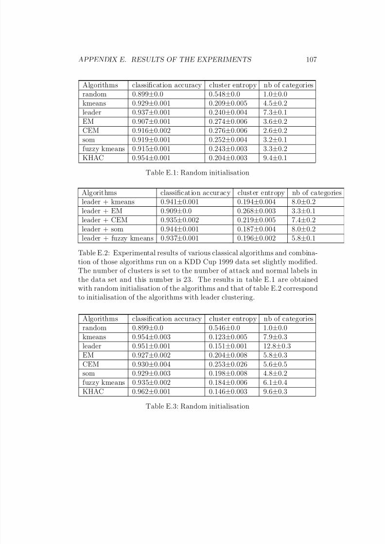
8/8/2019 Comp of Clustering Method
http://slidepdf.com/reader/full/comp-of-clustering-method 116/117
APPENDIX E. RESULTS OF THE EXPERIMENTS 107
Algorithms classification accuracy cluster entropy nb of categories
random 0.899±0.0 0.548±0.0 1.0±0.0kmeans 0.929±0.001 0.209±0.005 4.5±0.2leader 0.937±0.001 0.240±0.004 7.3±0.1EM 0.907±0.001 0.274±0.006 3.6±0.2CEM 0.916±0.002 0.276±0.006 2.6±0.2som 0.919±0.001 0.252±0.004 3.2±0.1fuzzy kmeans 0.915±0.001 0.243±0.003 3.3±0.2KHAC 0.954±0.001 0.204±0.003 9.4±0.1
Table E.1: Random initialisation
Algorithms classification accuracy cluster entropy nb of categoriesleader + kmeans 0.941±0.001 0.194±0.004 8.0±0.2leader + EM 0.909±0.0 0.268±0.003 3.3±0.1leader + CEM 0.935±0.002 0.219±0.005 7.4±0.2leader + som 0.944±0.001 0.187±0.004 8.0±0.2leader + fuzzy kmeans 0.937±0.001 0.196±0.002 5.8±0.1
Table E.2: Experimental results of various classical algorithms and combina-tion of those algorithms run on a KDD Cup 1999 data set slightly modified.
The number of clusters is set to the number of attack and normal labels inthe data set and this number is 23. The results in table E.1 are obtainedwith random initialisation of the algorithms and that of table E.2 correspondto initialisation of the algorithms with leader clustering.
Algorithms classification accuracy cluster entropy nb of categoriesrandom 0.899±0.0 0.546±0.0 1.0±0.0kmeans 0.954±0.003 0.123±0.005 7.9±0.3leader 0.951±0.001 0.151±0.001 12.8±0.3EM 0.927
±0.002 0.204
±0.008 5.8
±0.3
CEM 0.930±0.004 0.253±0.026 5.6±0.5som 0.929±0.003 0.198±0.008 4.8±0.2fuzzy kmeans 0.935±0.002 0.184±0.006 6.1±0.4KHAC 0.962±0.001 0.146±0.003 9.6±0.3
Table E.3: Random initialisation
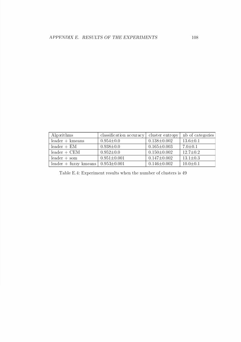
8/8/2019 Comp of Clustering Method
http://slidepdf.com/reader/full/comp-of-clustering-method 117/117
APPENDIX E. RESULTS OF THE EXPERIMENTS 108
Algorithms classification accuracy cluster entropy nb of categoriesleader + kmeans 0.954±0.0 0.138±0.002 13.6±0.1leader + EM 0.938±0.0 0.165±0.003 7.0±0.1leader + CEM 0.952±0.0 0.150±0.002 12.7±0.2leader + som 0.951±0.001 0.147±0.002 13.1±0.3leader + fuzzy kmeans 0.953±0.001 0.146±0.002 10.0±0.1
Table E.4: Experiment results when the number of clusters is 49