ISSN: 1962-5361Disclaimer: This Philadelphia Fed working paper represents preliminary research that is being circulated for discussion purposes. The views expressed in these papers are solely those of the authors and do not necessarily reflect the views of the Federal Reserve Bank of Philadelphia or the Federal Reserve System. Any errors or omissions are the responsibility of the authors. Philadelphia Fed working papers are free to download at: https://philadelphiafed.org/research-and-data/publications/working-papers.

Working Papers

Commuting, Labor, and Housing Market Effects of Mass Transportation: Welfare and Identification

Christopher SeverenFederal Reserve Bank of Philadelphia Research Department

WP 18-14Revised September 2021March 2018https://doi.org/10.21799/frbp.wp.2018.14

Commuting, Labor, and Housing Market Effects of MassTransportation: Welfare and Identification∗

Christopher Severen†Federal Reserve Bank of Philadelphia

September 2021

Abstract

I study Los Angeles Metro Rail’s effects using panel data on bilateral commuting flows, a quan-titative spatial model, and historically motivated quasi-experimental research designs. Themodel separates transit’s commuting effects from local productivity or amenity effects, andspatial shift-share instruments identify inelastic labor and housing supply. Metro Rail con-nections increase commuting by 16% but do not have large effects on local productivity oramenities. Metro Rail generates $94 million in annual benefits by 2000, or 12–25% of annual-ized costs. Accounting for reduced congestion and slow transit adoption adds, at most, another$200 million in annual benefits.

Keywords: subway, commuting, gravity, economic geography, local labor supplyJEL Codes: J61, L91, R13, R31, R40

∗Many have provided valuable advice during the development of this paper; I would especially like to thank ElliotAnenberg, Valerie Bostwick, Jeff Brinkman, Olivier Deschênes, Jonathan Dingel, Gilles Duranton, Jessie Handbury,Xavier d’Haultfœuille, Stephan Heblich, Kilian Heilmann, Nicolai Kuminoff, Jeff Lin, Kyle Meng, Yuhei Miyauchi,Paulina Oliva, and Wei You, as well as several anonymous referees.

Disclaimer: This working paper represents preliminary research that is being circulated for discussion purposes.The views expressed in this paper are solely those of the author and do not necessarily reflect those of the FederalReserve Bank of Philadelphia or the Federal Reserve System. Any errors or omissions are the responsibility of theauthor.†Address: Research Department, Federal Reserve Bank of Philadelphia, Ten Independence Mall, Philadelphia, PA

19106. Email: chris.severen@gmail.com or Chris.Severen@phil.frb.org.

1

1 Introduction

High commuting costs limit consumer choice and mobility within cities. Governments invest largesums in urban rail transit infrastructure to mitigate the costs of distance and congestion. What arethe benefits of these investments, and what margins of urban economic geography do they shift?

I study the effects of Los Angeles Metro Rail on commuting, non-commuting margins, andwelfare. I assemble data on census tract-to-census tract commuting flows in 1990 and 2000 anddevelop a new approach to measure the effects of transit on commuting using these flows. Iden-tification of the commuting effect exploits bilateral and panel aspects of the data. To study thenon-commuting effects of infrastructure and quantify welfare impacts, I describe a quantitativespatial general equilibrium model and develop a new strategy to identify its key parameters.

A panel gravity equation, which can be embedded in the model, estimates the commuting ef-fect of transit on bilateral flows. Instead of comparing single locations, identification hinges onselecting pairs of locations that satisfy treatment ignorability. This means comparing changes inflows between pairs of locations that both receive treatment to changes in flows between pairs oflocations in which just one, or neither, receives treatment. I leverage unanticipated shocks to routeconstruction, historical streetcar routes, and proposed subway lines to limit selection concerns.1

The commuting effect is substantial: flows increase 11%–16% between connected tract pairs thatboth contain stations by 2000. Tract pairs both slightly more distant from new stations see in-creases of 8%–14%; there is no effect farther away. I also find evidence of moderate medium-runcongestion improvements by 2000 and further commuting growth of 9%–12% between previouslyconnected tracts by 2015. These results suggest that latent demand may not fully displace reducedcongestion in the medium run, in contrast to the Fundamental Law of Congestion (Downs 1962).

The model distinguishes the commuting effect of transit from non-commuting effects. Non-commuting effects impact all residences or workplaces near a station, rather than just commutersusing transit-served routes. Conditional on model parameters, data on local housing and laborprices and quantities map to tract-specific and time-varying non-commuting fundamentals (e.g.,productivity, amenities). I then estimate the effect of transit on changes in these fundamentals witha differences-in-differences strategy, which controls for confounding time-invariant factors (e.g.,proximity to the coast). The commuting effect dominates; impacts from non-commuting channelsappear minimal.

The model quantifies welfare and accounts for general equilibrium adjustments. Panel data onaverage wage and industry mix at place of work identify key model parameters.2 Foremost is thelocal extensive-margin elasticity of labor supply to a tract, which governs how responsive agentsare to changes in prices, amenities, and commuting costs. It is also essential for translating treat-

1. See Redding and Turner (2015) for a review of this challenge and common solutions.2. Workplace wage is often unobserved. I use panel workplace wage data to test a key identifying assumption in

Ahlfeldt et al. (2015) meant to overcome unobserved workplace wage and find that is unlikely to hold precisely.

2

ment effects to welfare. Estimates indicate a low value, implying agents heterogeneous in theirpreferred locations and relatively unwilling to move in response to changes in local characteris-tics. I also interact local labor demand shocks with the spatial configuration of the city to estimatea tract-scaled housing supply elasticity.

By 2000, LA Metro Rail generates a baseline $94 million (in 2016 dollars) in annual surplus(12%–25% of the annualized cost) through commuting channels.3 A bootstrap 95% confidenceinterval of this benefit is 2%–64% of costs. Upper bounds on additional annual benefits are $132million from reduced congestion and $76 million from slow adjustment in commuting behavior.Back-of-the-envelope calculations of air pollution benefits may add $100 million annually. Thoughsubstantial, the commuting benefit alone of LA Metro Rail does not clearly exceed its cost over itsfirst two decades, highlighting the difficulty in shifting commuting behavior in restrictively zoned,car-oriented cities. Had zoning allowed 10% greater residential density near transit, the benefitsof transit would have doubled.

This approach bridges the hedonic method of valuing transportation infrastructure (e.g., McMillenand McDonald 2004) with a generalized form of the travel time-based method typical of quantita-tive urban models (e.g., Ahlfeldt et al. 2015; Monte, Redding, and Rossi-Hansberg 2018; Tsivanidis2018). The hedonic method gives a real estate-mediated measure of the overall effect of transit dueto both commuting and non-commuting margins, but cannot disentangle these margins nor ac-count for general equilibrium effects.4 In contrast, quantitative urban models often only allowtransit to shift commuter market access.

Panel commuting flow data offer a substantial improvement over common practice in the lit-erature, which relies on cross-sectional flow data to parameterize gravity models and infer marketaccess. The literature often interprets changes in travel times as perfectly determining changesin commuting flows. Instead, I directly use commuting flows, which reflect travel times but alsocapture any other hard-to-measure, route-specific characteristics of commute choice (e.g., pleas-antness or reliability). The panel aspect permits the use of pair-specific fixed effects, which controlfor the time-invariant components of these hard-to-measure characteristics. Moreover, commut-ing flow data obviate the need to estimate historical travel times from modern routing engines.

Los Angeles is a populous, car-oriented region that built an extensive rail network within adecade, so its experience may be more informative for many cities considering rail-based masstransit than evidence from older, denser cities. It is an active line of inquiry whether new masstransit infrastructure in less dense cities provides appreciable benefits, particularly given the newer

3. There are three important caveats. First, while I calculate the commuting effects over a 25-year window, I examineother channels only from 1990 to 2000 due to data limitations. Second, the welfare analysis assumes that agents havehomothetic preferences. Finally, transit may benefit non-commuting travel or have environmental effects on cities as awhole. I discuss these in Section 8.

4. Equilibrium effects (e.g., price spillovers) violate the stable unit treatment value assumption and can invalidate he-donic analysis. Donaldson and Hornbeck (2016) highlight the importance of equilibrium adjustments when evaluatingtransportation infrastructure.

3

role of cities as centers of consumption (Baum-Snow, Kahn, and Voith 2005). There is a buddingline of research examining the consequences of LA Metro Rail.5

I describe the setting and data in Section 2. Section 3 discusses identification and estimationof the commuting effect. Section 4 develops and characterizes the model. Section 5 addressesthe second empirical challenge: estimating the model’s elasticities. I describe estimating the non-commuting effects of transit in Section 6. Section 7 reports baseline welfare analysis, and Section8 discusses extensions and discusses broader conclusions.

2 Setting and Data: Transit in Los Angeles

Automobiles have long been a common feature of mobility in Los Angeles. Angelenos adoptedautomobiles in large numbers during rapid urban growth in the 1920s, leading to early complaintsof crowded streets and attempts to relieve traffic delays (Fogelson 1967). Increasing congestion inthe 1960s and 1970s led to several failed referendums to expand rail transit. By 1980, the situationreached a political tipping point and voters passed Proposition A—a sales tax increase to fund railtransit. The proposed plan combined heavy rail (subway) and light rail operations in an intercon-nected urban rail transit system. Construction on the system began in 1985 and the first light railline (the Blue Line) partially opened in mid-1990 (construction delays meant it did not reach itsurban termini until early 1991). The subway line faced routing difficulties and first opened in 1993.It was expanded in 1996 and 1999 and is now run as two lines: the Red and Purple Lines. Anotherlight rail line initially meant to connect to the international airport (the Green Line) opened in 1995largely in the median of a new freeway, but without reaching the airport.6

To study the effects of rail transit in Los Angeles, I develop a panel of tract-level variablesin 1990 and 2000 that covers Los Angeles County and four adjacent counties (Orange, Riverside,San Bernardino, and Ventura). This five-county area is economically distinct from nearby conur-bations and captures most relevant local interactions. I briefly discuss primary data sources andprocessing below; additional details can be found in the Appendix.

Geo-normalization. The standard unit of observation is a census tract or tract pair using 1990Census geography. I normalize to 1990 geography to minimize rounding errors. I areally weightmore recent geographies when crosswalking to 1990 tracts.

Commuting flow data. Tract-to-tract commuting flow data are primarily from the 1990 and2000 Census Transportation Planning Packages (CTPP). I normalize origin-destination pairs to1990 geography and apply consistent rounding and suppression rules to create a consistent panel.I also use commuting flow data covering 2002 and 2015 from the Longitudinal Employer-HouseholdDynamics Origin Destination Employment Statistics (LODES), normalized to 2010 geographies.

5. See, for example, Redfearn (2009), Schuetz (2015), and Schuetz, Giuliano, and Shin (2018).6. LA Metro Rail’s line names recently changed. I use the older designations for continuity. The system continues to

grow, with 6 lines, 93 stations, and 106 miles of rail as of 2016.

4

Due to methodological differences, CTPP and LODES data are not combined.Place of residence and place of work data. Data on residential census tracts and block groups

are from the National Historic Geographic Information System (NHGIS) and GeoLytics Neighbor-hood Change Database (NCDB). The CTPP contains tract of work wage data unavailable elsewhereand employment by industry in 18 aggregate Standard Industrial Classification (SIC) codes. I trimthe data to exclude implausible changes between 1990 and 2000 levels.

Transit data and treatment; other data sources. I combine geodata on Metro Rail transit sta-tions and lines from the Los Angeles County Metropolitan Transportation Authority (LACMTA)with published information on the timing of openings. To construct labor demand shocks, I useIPUMS microdata on all workers outside of California from the 1990 and 2000 Censuses. Panelland use data are from the Southern California Association of Governments (SCAG).

3 Commuting Effects of LA Metro Rail

The number of commuters from residential tract i to workplace tract j at time t, denoted Nijt,depends on residential tract characteristics, θit, workplace tract characteristics, ωjt, and trip char-acteristics τijt. Let T denote some function of proximity to transit. Commuting is:

Nijt = Nijt

(θit(Tit), ωjt(Tjt), τijt(Tit, Tjt)

). (1)

The commuting effect of transit isolates transit’s effect connecting i and j: ∂N∂τ

∂τ∂T . Transit can

generally shift residential or workplace characteristics as well. Comparing flows by T alone doesnot differentiate commuting effects from other margins.

Panel bilateral commuting flow data can separate these margins. Bilateral data allow flexiblycontrolling for residential and workplace characteristics and shocks, while temporal variation al-lows controlling for time-invariant pair-specific characteristics. Let Tijt denote proximity to transitat both i and j. I estimate:

ln(Nijt) = ωjt + θit + T ′ijtλD + x′ijtβ + dij + ιsisjt + dijt, (2)

where dij are pair fixed effects and dijt captures unobserved variation in commuting betweenlocations over time.7 Residential and workplace tract-by-year fixed effects, θit and ωjt, capturenon-commuting effects of transit.

Equation (2) is a panel gravity equation, wherein the pair fixed effects subsume distance.8

7. While the structural model interprets dijt as an unobserved utility shifter, Dingel and Tintelnot (2020) highlighthow granularity can produce measurement error.

8. Nijt = 0 for some observations, so ln(Nijt) is undefined. I estimate high-dimension fixed-effects Poisson PMLmodels to show robustness (Larch et al. 2019). Results are broadly consistent, as only tract pairs that are zero in oneperiod and non-zero in the other period can lead to differences (always-zero pairs separate out).

5

These fixed effects also capture unobserved determinants of commuting flows—such as bus ser-vice, ease of parking, pleasantness, or even workplace-residential matching—to the extent thatsuch features are time invariant. Some specifications use subcounty-by-subcounty-by-year fixedeffects (ιsisjt) to capture regional shifts in commuting patterns and allow flexible trends in regionalintegration. In xijt, I include time-varying measures of proximity to the Century Freeway, whichopened in the mid-1990s.

Treatment, Tijt, reflects three mutually exclusive, binary definitions of proximity of both a resi-dential and a workplace tract to LA Metro Rail stations open before the end of 19999:

i) O & D contain station: Both tracts either contain a transit station or have their centroid within500 meters of a transit station.

ii) O & D <250m from station: Both tracts have some part within 250 meters of a transit station,but i) is not true.

iii) O & D <500m from station: Both tracts have some part within 500 meters of a transit station,but neither i) nor ii) is true.

3.1 Identification

Equation (2) estimates a dyadic difference-in-differences (DD) design supplemented with origin-and destination-by-year fixed effects. Interpreting λD as the average causal effect of LA Metro Railon commuting flows requires assuming parallel counterfactual trends: In the absence of treatment,commuting between treated and control tract pairs would have evolved similarly on average, con-ditional on separable changes to residential and workplace locations. This substantially relaxes standardDD assumptions. Time-varying origin and destination fixed effects largely control for confound-ing factors (e.g., school quality, zoning).

While nonrandom siting of transit threatens the parallel trends assumption, origin and desti-nation fixed effects remove concerns about where stations are placed. I limit pair-specific selectionconcerns with two approaches. First, I use historical data giving the locations of a proposed sub-way network and former streetcar lines, which embeds shocks to route placement and thus selectspairs of tracts that share common historical trends and could have both plausibly been treated by2000. The second approach considers only tract pairs that are both near existing or not-then-builttransit stations, comparing pairs along the same subway line with pairs that are not.

History & Shocks designs. Kelker, De Leuw & Co. (1925) designed a rail transit network toaccommodate Los Angeles’ booming population in the 1920s (the plan was shelved partly becauseof skepticism of rail companies and a preference for tunneled lines).10 The plans also show former

9. For a hypothetical square tract of median area (1.38km2) with a uniformly distrbuted population, average distanceto a station for each proximity is i) 444m–888m, ii) 689m–888m, and iii) 901m–1219m; see Appendix A.4.

10. The relevant maps from Kelker, De Leuw & Co. (1925) are shown in Appendix Figure H1.

6

Pacific Electric Railroad (PER) lines, an at-grade passenger rail system. I define two samples asthe union of tract pairs near LA Metro Rail by 2000 and pairs that lie near: (i) the Kelker, De Leuw& Co. (1925) subway proposal, “1925 Subway Plan”; or (ii) PER lines, “PER Sample”. The 1925Subway Plan itself has two variants: an “Immediate” plan meant for immediate construction, anda plan meant to accommodate buildout (“All”). These research designs are mapped in Figure 1.

The validity of these groups as controls is supported by several lines of reasoning and evi-dence. First, many control pairs contain one “end” (either the origin or destination) that is treated,though the other end is not. Such control pairs compare changes in the number of commutersresiding in iwho work in j (which receives a transit linkage) to the number who work in j′ (whichdoes not). Similarly, workers in j who reside in i are compared with those who reside in i′. Thesecomparisons control for many potential unobserved motives for changing commuting behavior.

Second, control tracts selected by this approach are near historical transit corridors, as aretreated locations. Brooks and Lutz (2019) show that locations near former streetcar routes in LosAngeles are generally on similar land use trajectories. This promotes viability of transit siting, andland use itself can have an impact on travel behavior (Duranton and Turner 2018).

Third, there was significant variation in the timing of route construction due to reasons likelyorthogonal to transit demand. Notably, a geologic shock limited westward expansion of theRed/Purple Line (its original routing was along Wilshire Boulevard, one of the densest corri-dors in Los Angeles). Methane seeping into a nearby clothing store exploded in March 1985. Eventhough the explosion was not related to subway construction, legislation soon restricted tunnelingalong Wilshire. This corridor is served by transit in both the 1925 Subway and PER samples, andin almost every plan since. Similarly, the Green Line’s route was built partially within an under-construction highway to minimize construction costs. Its westward end was meant to serve LosAngeles International Airport (LAX), but the Federal Aviation Administration’s concerns aboutelectromagnetic interference detoured this alignment to the south. Construction is underway onconnections between the system and the Wilshire corridor and LAX, so these shocks can be seenas generating plausibly exogenous variation to the timing of treatment.

Routes also reflect other non-transportation concerns, such as satisfying political pressures,ensuring political support for transit revenue allocations, and spurring political favor from com-peting oversight agencies.11 To illustrate, politicians demanded that heavy rail serve the San Fer-nando Valley, despite the cost and difficulty of doing so. It was also deemed necessary to connectLong Beach to ensure access to its portion of state gas tax revenue. At one point, a particularlyserpentine route was dubbed the “wounded knee” because it touched so many local political ju-risdictions. In sum, Elkind (2014, p. 50)’s statement that “politics, outside circumstances, and thegeography of power . . . played an outsized role in influencing where the new rail lines would go”

11. The political setting is presented in Elkind (2014), who notes that “plotting a subway through the politically de-centralized landscape of Los Angeles meant ceding control to numerous fiefdoms of federal, state, and local politicians”(p. 70).

7

indicates the presence of factors unrelated to travel demand in the planning process.Finally, I provide econometric evidence. While the data do not permit testing pre-trends in

tract-pair flows, I examine pre-trends in tract-level housing and labor market characteristics usingNCDB data from 1970 to 1990.12 Among economic variables later captured in the model (columns1–4 of Appendix Table H2), there are no significant differences in pre-trends in employed popula-tion or household income in any sample; there is marginal evidence of pre-trends in housing val-ues and number of households. However, the Immediate 1925 Subway Plan specification showsno evidence of differential pre-trends in model-relevant characteristics, and so is preferred.

I also investigate differential trends in neighborhood and travel characteristics (columns 5–10of Appendix Table H2). In some samples, residents of treated tracts were becoming less collegeeducated and more impoverished and were moving less often. Evidence on differences in travelpre-trends is mixed: in two samples, the share of household with no cars was decreasing prior totreatment. In none of the samples was the commuting share by auto differentially changing, butin all samples the relative transit commuting share transit was increasing slightly. The Immediate1925 Subway Plan sample shows the least evidence of pre-trends across all variables.

Recall that the fixed effects in Equation (2) render it robust to any tract-level pre-trends, whetherobservable or not. While tract-level pre-trends do not impede identification of the commuting ef-fect, they may confound the non-commuting analysis in Section 6.

Same Line designs. These designs compare tract pairs on the same line to tract pairs that lie alongdifferent lines. This design expects that tract pairs along the same line are “more treated” thanthose that are not. Parallel trends are violated if planners targeted directly connecting (by thesame line) locations that would have seen larger increases in commuting anyway relative to othertreated—but indirectly connected—locations. I consider two variants. The first includes locationstreated by 2000 and locations not yet treated in 2000 but that are treated by 2015. In this ‘EverTreated’ variant, treated pairs both lie near stations along the same line and control pairs both lienear stations open by 2015 but that are not along on the same line. In the second, more stringentvariant (Treated by 2000), I restrict control pairs to those that lie near a station open by 2000.

There are two caveats regarding these designs. First, they identify the commuting effect oftransit only if it is infinitely costly to switch from one line to another (i.e., a very high transferpenalty). Under a finite (but non-zero) transfer penalty, these designs reflect the marginal effectof being directly connected relative to being indirectly connected. Second, these designs rely onfewer observations and are less precise.

12. NCDB is, by default, normalized to 2010 geographies. I use the same treatment rules, but this results in higherobservation counts due to denser tracts in 2010 than 1990.

8

3.2 Commuting flow estimates

Panel A of Table 1 reports estimates of λD on commuting flows between 1990 and 2000. Columns1–3 show results from the full sample, successively adding in measures of treatment proximity,subcounty pair-by-year fixed effects, and controls. Columns 4–6 reflect the History & Shocksdesigns. Columns 7–8 report results from the Same Line designs. Clustered standard errors arerobust to correlation within tract pairs, residential tracts, and workplace tracts.

LA Metro Rail increased commuting 10%–22% between tracts nearest transit stations by 2000.Estimates are significant across all specifications. The preferred specification (column 6) indicatesan increase of 14.9 log points (16%). Slightly fewer transit-proximate tract pairs see an effect of8%–14%, with a preferred estimate of 12.8 log points (14%). Tract pairs at a farther distance fromstations see no significant effect.13

Several features of the results are reassuring. First, estimates are ordered by proximity. To-gether these form a specification test: effects should concentrate near stations with little no effectfarther away. Second, as the control group becomes more targeted (and sample size decreases),point estimates become larger (ascending from left to right). This ordering implies that controltract pairs experience progressively less commuting growth than in the full sample. As thesedesigns increasingly select connections between older, more mature parts of the city, this is rea-sonable. Finally, Same Line estimates are a bit larger than the History & Shocks estimates, but alsoless precise. This suggests that proximity to directly connected stations is more important thansimply being near a transit station.14

Panel B of Table 1 extends the analysis to determine if there are additional effects from 2002–2015 using LODES data. Because LA Metro Rail expanded during this period, I estimate a variantof Equation (2) with two different effects: Existing connections for the additional increase betweentracts connected by stations built earlier (between 1990 and 2002), and New connections for stationsbuilt after 2002. Existing connections experience additional commuting growth of 8%–12% by 2015if both tracts were previously connected and 5%–10% if the tracts were a bit farther from stations.New connections increase commuting by 10%–14% between tracts that both contain new stationsby 2015 and up to 9% for those slightly more distant from stations. While substantial, these effectsare likely smaller than for tracts connected between 1990 and 2000 because stations built between2002 and 2015 are generally more suburban.

13. See footnote 9 for interpretation of these distance bins and robustness in Appendix Figure H6. Similar estimatesresult from Poisson PML specifications; see Appendix Table H4.

14. Appendix Table H5 directly tests this. Though noisy, effects are always for locations along the same line. Thedata allow further exploration in this vein. Interacted proximity bins for origin and destination tracts indicate a greatereffect of proximity at the destination than the origin, suggesting commuters respond more to closer workplace-to-station proximity than to closer residence-to-station proximity (Appendix Table H6). Treatment does not generallyalter the extensive margin of connection, but its effect may increase slightly over time (Appendix Table H3).

9

3.3 Commuting time (congestion) estimates

A common motivation for rail transit is to relieve automobile congestion. Anderson (2014) findsthat a 2003 labor strike that disrupted LA Metro Rail service increased nearby automobile conges-tion by 47%. However, that strike lasted 35 days. It is unclear how to map that short-run responseto the long run. Duranton and Turner (2011) find no aggregate evidence that transit decreases au-tomobile travel. This notion, called the “Fundamental Law of Congestion” (Downs 1962), suggeststhat congestion improvements (and downstream benefits like air pollution) may be transitory.

I combine reported CTPP travel times with inferred travel routes to test for decreased con-gestion due to transit.15 I map the fastest driving route between all location pairs in my sampleand calculate the share of each route (`ij∈k/`ij) that falls within five mutually exclusive distancebuffers k (omitting the share of the route more than 4km distant). I then estimate:

ln(τijt) =∑k

λτ,k`ij∈k`ij

1[t=2000] + ωjt + θit + ςij + εijt, (3)

where τijt is the average reported travel time from i to j in year t.Table 2 shows results for two measures of travel time: log travel time across all modes and log

travel time for private cars. Results for all-mode travel times are negative but mostly insignificant;they may reflect mode switching to transit. Car-only results, however, show clear evidence of areduction in travel time.16 Routes that are entirely within 250m meters of lines by 2000 see a 15.0log point (14%) reduction in travel time. For routes lying entirely 250m–500m from lines by 2000,travel times decrease by 18.9 log points (17%). Though not statistically different, the larger effectslightly farther from the rail lines may indicate slower travel due to at-grade crossings. Portionsof routes that lie farther than 500m from a rail line see no change in travel times.

The estimates in columns 3–4 of Table 2 are roughly one-third those in Anderson (2014). Thissuggests substantial but incomplete attenuation of congestion benefits over a period of 5–10 years,indicating that congestion benefits of transit may not be entirely transitory. Any downstreambenefits, like improved air quality, may similarly last over longer time horizons.

4 A Model of Urban Location Choice

I turn to a quantitative urban model of residential and workplace choice to recover the non-commuting effects of transit and translate the effects of transit to welfare. The model links local,observable equilibrium outcomes to local, unobservable economic fundamentals (e.g., productiv-

15. The setting is comparable to Anderson (2014), though he uses a different research design and focuses primarilyon observed highway travel speeds. See Brinkman (2016) and Allen and Arkolakis (2019) for endogenous congestion.

16. Sample sizes are smaller than in Table 1 due to disclosure restrictions, which is also why the sample for privatecar travel time is yet smaller. I also drop pairs for which the implied trip speed is greater than 80mph.

10

ity, amenities). The model includes a collection of N locations in a city, operationalized as censustracts, that each contain a labor market and a housing market.17

Joint market household decision: Labor supply and housing demand

Atomistic households make consumption decisions and choose a tract of work and a tract of resi-dence. Conditional on residential location i, households face per-unit housing costsQi and receiveamenity Bi. Conditional on place of work j, households inelastically provide one unit of labor inexchange for wage Wj . Given locations and prices, households make decisions over consumptionof housing and a composite good. Specifically, household o chooses location pair ij, consumptionC, and housing H to maximize Cobb-Douglas utility:

maxC,H,ij

Uijo = maxC,H,ij

νijoBiδij

(Cζ

)ζ ( H

1− ζ

)1−ζs.t. C +QiH = Wj ,

where νijo is household o’s idiosyncratic preference for location pair ij. The commuting costbetween i and j is captured by δij ≥ 1. The share of household expenditures on housing is 1 − ζ.Indirect utility conditional on location pair ij is:

vo|ij =νijoBiWjQ

ζ−1i

δij.

Housing consumption for o conditional on ij is Hijo = (1− ζ)Wj/Qi.I assume νijo is distributed Fréchet with scale parameter Λij = TiEjDij and shape parameter

ε > 0. The CDF of ν is thus: Fij(ν) = eTiEjDijν−ε

. The scale parameter captures mean idiosyncraticpreference for location pair ij: Ti captures the mean utility of residing in i, Ej the mean non-wage utility of working in j, and Dij an unobserved pair-specific shift in the utility of a particularcommute. The shape parameter governs the degree of homogeneity in preferences: For high ε,agents view location pairs homogeneously, while for low ε, their valuations are heterogeneous.The share of the population that chooses residential location i and place of work j under theFréchet assumption is:

πij =Λij

(δijQ

1−ζi

)−ε(BiWj)

ε∑r

∑s Λrs

(δrsQ

1−ζr

)−ε(BrWs)ε

. (4)

17. The model is similar to Ahlfeldt et al. (2015), with five differences: (i) origin-destination pairs can differ in meanutility, which permits deriving Equation (2) from the model; (ii) a local housing efficiency parameter captures differ-ences in local regulations and per unit housing costs; (iii) land use between housing and production is exogenouslydetermined; (iv) endogenous externalities are omitted (though I discuss model variants with endogenous agglomera-tion for welfare calculations in the Appendix); and (v) the model can be written as a system of three equations log-linearin data and fundamentals.

11

Observable commuting flows are Nij = πijN , where N is total population.The city can be viewed as either existing in autarky or being nested in a large, open economy.

This assumption makes little difference outside of welfare calculations (due to homothetic prefer-ences). In an open economy, no spatial arbitrage requires that the average welfare from moving tothe city equal the reservation utility of living elsewhere, so:

E[Uijo] = Γ

(ε− 1

ε

)·

[∑r

∑s

Λrs

(δrsQ

1−ζr

)−ε(BrWs)

ε

]1/ε

, (5)

where Γ(·) is the gamma function and the aggregate population N is given or implicitly defined.Under free mobility E[Uijo] = U and aggregate population changes to maintain U .

Production: Labor demand

Measure-zero firms produce a globally tradable commodity in each location j under perfect com-petition. Firms select labor NY and land LY inputs to maximize profits under constant returns toscale. Production is multiplicatively separable in local productivity Aj and a technology that isidentical across j: Y = AjF (NY

j , LYj ). Because of the atomistic size of firms, land use decisions are

made in accordance with profit maximization despite the locally fixed quantity of land. Perfectcompetition in labor markets implies that firms pay workers the marginal product of labor: Wj =

AjFN (NYj , L

Yj ). I assume Cobb-Douglas production technology: F (NY , LY ) = (NY )α(LY )1−α.

Inverse labor demand is given by:

Wj = αAj(LYj /N

Yj

)1−α. (6)

Housing supply

Measure-zero builders construct housing using land LH and material inputs M . A local, multi-plicatively separable housing productivity term Ci captures cost drivers such as geography andregulation. Materials are readily available in all locations at the same cost, but local land supplyfor housing is predetermined.18 Convexity in land pricing serves as a congestive force, driving upprices in desirable locations until agents look elsewhere. I specify Cobb-Douglas housing produc-tion: H = (LH)φM1−φCi. Developers sell housing in location i in a competitive market at unitprice Qi to maximize profit: QiH − PLi L

H − PMM . The price of construction materials PM isexogenous and common to all locations.

Because detailed data on housing production are not available, I utilize a zero-profit conditionto develop an empirical formula for housing costs. The first-order condition for developer profits

18. This simplifies the model while maintaining fidelity to the setting. Strong zoning and the medium-run time frameof this study may not match the temporal patterns required for land use change.

12

with respect to construction materials gives:

Qi =PM

(1− φ)Ci

(M

LH

)φ. (7)

Substituting this into the developer’s profit function and enforcing zero-profit conditions gives

construction material demand,M∗ = 1−φφ

LHPLjPM

, as well asQi = (PLi LH+PMM)/((LHi )φM1−φCi).

Substituting in M∗ gives the cost function: Qi = Ci(PLi )φ, where Ci = (PM )1−φ/(1 − φ)1−φφφCi

captures the inverse efficiency in housing production.The price of land, PLi , responds to changes in demand and land availability: I parameterize it

as a function of local housing density PLi = (Hi/LHi )ψ, where the parameter ψ > 0 captures local

price elasticity of land with respect to density. This parameter provides a congestive force to themodel. Combining the expression for land price with Equation (7) relates housing supply, price,and land availability:

Qi = Ci(Hi/L

Hi

)ψ, (8)

where ψ = ψφ. As housing productivity Ci increases, Ci falls, so increases in housing productivity(decreases in Ci) increase the quantity of housing supplied at any price.

Equilibrium characterization

In equilibrium, labor and housing markets clear in all locations. Labor market clearing requiresthat demand equal supply locally:

NYi =

∑r

Nπri. (9)

Given Cobb-Douglas preferences, housing demand is a constant fraction of the ratio of wage tohousing price. Aggregate housing demand in i is the sum of wage-rent ratios weighted by com-muting flows, reflecting heterogeneity in income stemming from variation in wage (i.e., place ofwork). Housing market clearing requires that the local housing supply equal demand:

Hi = (1− ζ)∑s

NπisWs

Qi. (10)

Given model parameters α, ε, ζ, ψ, reservation utility U , vectors of land availability by useLY,LH, vectors of residential fundamentals B,C,T, vectors of place of work fundamentalsA,E, and matrices of commuting fundamentals and costs D, δ, an equilibrium is referencedby price vectors W,Q, commuting vector π, and scalar population measure N . Existence anduniqueness conditions are (proofs are in Appendix B):

Proposition 1. Consider the equilibrium defined by Equations (4), (6), (8), (9), (10):

13

i) At least one equilibrium exists for residential tracts with strictly positive quantities of residential landand work tracts with strictly positive quantities of land used in production.

ii) There is at most one equilibrium if

2ε(ε+ 1)(1− α)(1− ζ)

1 + ε(1− α)− 1 ≤ 1

ψ. (11)

Inversion

Though the model may have multiple equilibria, for a given set of parameters, there is a uniquemapping from the observed data to local fundamentals. Model parameters are estimated usingthese fundamentals and the observed values of the endogenous variables in combination withinstruments to define moment conditions. Bi and Ti enter isomorphically; let Bi = TiB

εi and

Λij = BiEjDijδ−εij .19 Local fundamentals A, C, and Λ can be expressed as unique functions of

data and parameters:

Proposition 2. Given parameters α, ε, ζ, ψ and observed data W,Q,π, N, a unique set of funda-mentals A,C,Λ exists and is consistent with the data being an equilibrium of the model.

5 Model Identification and Estimation

Local labor and housing market elasticities provide a mapping between local fundamentals (andinterventions that shift them) and observed prices and quantities. Consistent estimates of theelasticities are required to use observable data to learn about changes to local fundamentals andto simulate counterfactual scenarios. I develop an identification strategy that uses panel variationin wages at place of work, housing prices, and commuting flows, permitting the use of fixed effectsto control for unobserved, time-invariant characteristics that confound identification (for example,location near a port, on a pleasant hillside, or in town with stringent land use regulations).20

All components of the model are expressed in the commuting flow (4), wage setting (6), andhousing price (8) equations. Denote log values in lowercase letters. Adding time subscripts, in-cluding tract and tract-pair fixed effects (e.g., ln(Ajt) = aj+ajt), and letting nYjt be log employmentdensity, hit be log housing density, the g be constants, α = α−1, and ζ = −ε(1−ζ), these equations

19. This mapping diverges from Ahlfeldt et al. (2015). Note that the components of Λ are not uniquely identified fromthe data; I use statistical arguments to separate B, E, and Dδ−ε.

20. Persistent, difficult-to-measure amenities play an anchoring role in cities (Lee and Lin 2018). Strong land useregulation likely locks in such anchors in Southern California (Severen and Plantinga 2018).

14

deliver a tractable system log-linear in data and fundamentals (see Appendix B):

Labor demand: wjt = g0t + αnYjt + aj + ajt (12)

Commuting: nijt = g1t + εwjt + ej + ejt︸ ︷︷ ︸= ωjt,

Labor supply

+ ζqit + bi + bit︸ ︷︷ ︸= θit,

Housing demand

+dijt (13)

Housing supply: qit = g2t + ψhit + ci + cit (14)

Local fundamentals are potentially functions of covariates (aj + ajt = a(xjt) and so on), suchas transit proximity. Equation (13) interprets Equation (2) structurally, with fixed effects ωjt =

εwjt + ej + ejt and θit = ζqit + bi + bit, and utility-equivalent commuting costs such that dijt =

T ′ijtλD + x′ijtβ + dij + ιsisjt + dijt.

5.1 A general approach to identifying local elasticities

I develop a local shift-share instrument to overcome simultaneity in Equations (12)–(14). I leveragetract-level variation in shocks to labor demand, interacting these with the distance between tractsto create variation in local economic shocks. I focus on identification of ε (the elasticity of laborsupply) and ψ (the inverse elasticity of housing supply), as these embed information about thelocal economic environment and cannot be calibrated from microdata.21

Identification requires a demand or supply shock that shifts one of Equations (12)-(14) butis excludable from the others. I construct tract-level labor demand shocks from changes in na-tional wage and employment levels and ex ante local employment shares by industry. Effectivevariation comes from changes in wages and employment determined by ex ante local industrialcomposition. These shocks are relevant if correlated with changes in local productivity (∆ajt) andexcludable if uncorrelated with changes in other local fundamentals. Under these assumptions,labor demand shocks trace out the labor supply curve. Housing demand nearby shifts in response.Because this downstream response will be stronger nearer the workplace origination of the shock,I take a linear combination of labor demand shocks with weights determined by spatial decay andcommuting to map labor demand shocks to a residential tract and trace out the housing supplycurve.

Let Rq,Natt be average national wage or total national employment in industry q in year t, N qj,0

be the number of workers in each two-digit SIC industry q in the initial year (1990) in tract j, andNi,0 =

∑qN

qj,0 the ex ante total employment in tract i. The labor demand shock sums interactions

21. I also develop moment conditions that can identify all housing and labor demand elasticities in Appendix D,which exploit further interactions of city geography and local economic shocks.

15

of changes in wages or employment with ex ante employment shares across industries:

∆zjt =∑q

Rq,Natt −Rq,Nat0

Rq,Nat0

·N qj,0

Nj,0.

Because the demand shock embeds information on ex ante industry shares, an implicit identifica-tion assumption is that changes in non-productivity latent variables (e.g., amenities) are uncorre-lated with prior industry structure. To ensure that local factors do not drive national changes, Iexclude all workers in California.

5.2 The labor supply elasticity (Fréchet shape parameter)

The shape parameter ε governs the homogeneity of location preference and is an extensive-marginlabor supply elasticity that conditions on commuting and residential geography. I estimate ε usinga two-step strategy. In the first step, I recover ωjt from Equation (13) estimated by either a linearmodel or Poisson PML. In the second step, ωjt is the dependent variable in the wage equation:∆ωjt = ε∆wjt + ∆ejt. Instrumenting wage with the labor demand shock zjt identifies the laborsupply elasticity if:

E[∆zjt ×∆ejt] = 0, ∀j. (M-1)

Moment condition M-1 requires that the labor demand shock in a tract j be uncorrelated withunobservable changes in factors that shift labor supply to that tract, such as workplace-specificamenities or accessibility to tract j.22 Place of residence-by-year fixed effects (θit) control for anychanges in residential amenities that may be correlated with labor demand shocks.

Table 3 shows results using three different methods of recovering ωit instrumenting with thewage variant of the labor demand shock. Columns 1–2 estimate ωit jointly using both years of datain a log-linear panel. Columns 3–4 use a separate Poisson PML model for each year to estimateωit, conditioning on bilateral travel costs. Columns 5–6 jointly use both years of data, but with aPoisson PML estimator and pair fixed effects. As such, columns 3–4 include all tract pairs withzero flows, columns 5–6 drop tract pairs that have zeros flows in both time periods, and columns1–2 omit tract pairs with zero flows in any years (see footnote 8).

The first stage is significant, has the right sign, and is of a reasonable magnitude across all spec-ifications.23 Using the log-linear estimator of ω, estimates of ε are about 1. Unlike the commutinganalysis, zeros matter because any individual tract may have many incoming zeros. Estimates ofε based on ω from Poisson PML models vary between between 2.18 and 2.90. The inclusion of

22. Any differences in ∆dijt that apply to tract j as a whole confound ωjt and potentially contaminate ejt.23. The first stage captures the transmission of national wage shocks to local wages, so a value near 1 is expected.

A robust bootstrap 95% confidence interval is [0.562, 8.856] with a median value of 2.157; see Appendix E. AppendixTables H7 and H8 provide specification tests from Goldsmith-Pinkham, Sorkin, and Swift (2020) that correspond tocolumns 5–6 of Table 3.

16

subcounty-by-year fixed effects in columns 4 and 6 identifies the effect more narrowly from sub-regional variation. I take ε = 2.18 from Column 6 as the preferred estimate. The generally lowvalue of ε implies that workers are quite heterogeneous in location preferences and is roughly inline with extensive-margin labor supply elasticities found in studies of labor markets: Falch (2010)estimates labor supply elasticities between 1.0 and 1.9, Suárez Serrato and Zidar (2016) find valuesbetween 0.75 and 4.2, and Albouy and Stuart (2020) recover 1.98.

M-1 is a local, rather than citywide, moment condition, and is weaker than standard applica-tions of shift-share labor supply instruments. When a citywide labor demand shock is used totrace out labor supply, identification requires the shock be orthogonal to non-wage determinantsof labor supply (i.e., E[∆zt · (∆bt + ∆dt + ∆et)] = 0, where · averages over locations within a city).This suggests potential pitfalls in standard applications of shift share instruments. First, changesin residential amenities, commuting costs, and workplace amenities must be uncorrelated withlabor demand shocks regardless of where in the city they occur. Second, changes in amenities cannotbe correlated with the labor demand shock, whereas in my design, even unobserved and time-varying residential amenities are not confounding. Finally, in the standard design, changes incommuting costs cannot be correlated with labor demand shocks locally or elsewhere within thecity.

The urban economic geography literature often identifies ε from a combination of modelingassumptions and cross-sectional variation in travel time. Because I observe workplace wage, Ican test a prominent assumption. Ahlfeldt et al. (2015) select ε to rescale the variance of model-implied wages.24 This implicitly disallows positive correlation between w and e, and requireseither (i) E[wjej ]/V[ej ] = −1/2ε or (ii) V[ej ] = 0.25 Panel C of Table 3 presents tests of (i), whereestimates of ε from Panel A are enforced to calculate ej = ωj − εwj . Most specifications show anegative correlation between wj and ej , as required if E[wjej ]/V[ej ] = −1/2ε. The first row ofp-values treats ε as a constant, the second as a random variable (see Appendix D for details). Ifε is fixed, most specifications reject the null hypothesis that E[wjej ]/V[ej ] = −1/2ε. However, ifuncertainty in ε is taken into account, only Columns 3 and 4 reject the null.

Supplementary results in Appendix D indicate that wages explain only a relatively smallamount of the variation in workplace fixed effects ω. Similarly, Kreindler and Miyauchi (2020)—who also observe workplace wage—find only a modest cross-sectional relationship. Together,these results highlight the importance of carefully considering the relationship between workplace

24. Other papers take varied, ad hoc approaches to unobserved workplace wages. For example, Monte, Redding, andRossi-Hansberg (2018) assume an elasticity of substitution σ, specify a trade-in-goods model to recover productivityfrom cross-sectional trade flows, then assume recovered productivity is orthogonal to workplace and origin-destinationspecific amenities E[aj(σ)× (ej + dij)] = 0, ∀i, j, implicitly requiring correct model specification.

25. To see this, Ahlfeldt et al. (2015) require V(ωj) = V(wj), where ω = wj + 1εej , wj are model-implied wages, and

V(wj) is the variance of average wage across twelve districts of Berlin. Rearranging, noting that ej is mean zero, andsubstituting observed wage wj for wj and wj yields 2εE[wjej ] + V[ej ] = 0. Consider three cases: (i) if wj and ej arenegatively correlated, E[wjej ]/V[ej ] = −1/2ε; (ii) E[wjej ]⇔ V[ej ] = 0; and (iii) positive correlation wj and ej imply anegative variance of e.

17

wages and workplace amenities. While the variance assumption used to identify ε in Ahlfeldt etal. (2015) is unlikely to hold precisely or be universally reasonable, it may not be unreasonablewhere wj and ej are expected to have moderate negative correlation.

5.3 The (inverse) housing supply elasticity

A labor demand shock in one location shifts demand for housing in locations where workersmight live, and thus can be used to identify the slope of the housing supply curve. To map labordemand shocks to residential housing shocks, I use linear combinations of shocks ∆zHDit = zt ·ϑi,with weights ϑ that decay in travel time between locations that ever have positive commuting:

∆zHDit (ρ) =∑s

e−ρϑis1nis>0∆zst∑s e−ρϑis1nis>0

,

where ϑjs is the travel time between j and s, ρ is spatial decay, and nis denotes the maximumflow value from i to s in any year. With ρ > 0, labor demand shocks nearer a residential locationi are more important than labor demand shocks farther from i. The resulting inverse-travel timeweighted labor demand shock can be used to instrument housing density and identify ψ, theinverse price elasticity of housing supply, under the following condition:

E[∆zHDit (ρ)×∆cit] = 0, ∀i. (M-2)

Although both elements of M-2 relate to tract i, the housing demand shock draws on labor demandshocks from any j (including i).

M-2 requires labor demand shocks be uncorrelated with changes in (inverse) housing pro-ductivity, ∆cit, which reflects the efficiency of housing provision. One potential concern withAssumption A-2 is whether local zoning responds to local labor demand shocks. An alternativeversion drops the most local component of the labor demand shock (from i itself):

∆zHD,ait (ρ) =∑s 6=i

e−ρϑis1nis>0∆zst∑s 6=i e

−ρϑis1nis>0.

This identifies housing supply if E[∆zHD,ait (ρ) × ∆cit] = 0, ∀i, which is more easily parsed as afunction of the labor demand shock itself:

kijE[∆zjt ×∆cit] = 0, ∀ i 6= j, (M-2a)

where kij = e−ρϑij1nij>0 is a weight. Condition M-2a requires that innovations in housing effi-ciency be uncorrelated with nearby productivity shocks.

Implementing these moment conditions requires choosing the spatial decay parameter, ρ > 0,

18

governing how labor demand shocks propagate across space. I experiment with different values inln(ρ) ∈ [−10,−2]. I report results for ln(ρ) = −5.5, estimated in differences using the employmentinstrument. Table 4 estimates the inverse housing supply elasticity in Equation 14 under M-2 (oddcolumns) and M-2a (even columns). First stage estimates (panel D) are significant and negative,indicating that a positive productivity shock decreases nearby residential density. Productivityshocks increase per worker demand for residential floorspace, which—given restrictive zoning inthis area—either manifests as larger (likely single-family) homes or drives residential mobility toless dense housing options.

Estimates imply supply elasticities of 0.45–0.46 without income-driven adjustment in quan-tity (columns 1 and 2), and 0.57–0.62 when income can influence housing quantity (columns 3–6). Columns 3 and 4 provide a specification test for Equation (8).26 Even columns exclude theown-tract labor demand shock when aggregating the instrument (under M-2a); this permits localhousing productivity to covary with the local labor demand shock. Estimates are similar. Resultssuggest that local, tract-level housing provision is inelastic from 1990 to 2000. While Saiz (2010)finds the population-weighted housing supply elasticity in large U.S. cities is 1.75, the estimate forthe Los Angeles area is 0.63, which is very close to the results in columns 3–6 of Table 4.

6 Non-commuting Effects of Transit

Given parameters ε, ψ, α, ζ and data on workplace wages, residential housing prices, and com-muting, the model delivers straightforward expressions to recover local economic fundamentals—they are the model residuals A,B,C,E.27 These economic fundamentals represent economiccharacteristics of a place that exist outside of a market equilibrium. In combination with marketforces, fundamentals determine equilibrium prices and the distribution of people.

Because these residuals embed information on local fundamentals, they can be used to studythe effects of policy. Consider a local intervention, T . In general, the intervention could impactany local fundamental. I model the effect of T on fundamentals with panel data as

Yit = λTit + ςi + εit, (15)

where λ = λA, λB, λC , λE are the effects to be estimated and Y = a, b, c, e are the logged(non-commuting) fundamentals. Standard research designs can be used to identify λ (the fullsample should be used to estimate the structural elasticities, but intervention effects may use a

26. The coefficients in columns 3–4 in Table 4 should be equal in magnitude and opposite in sign. They are notstatistically different in absolute value (Panel C). A robust bootstrap 95% confidence interval is [1.008, 3.672] with amedian value of 1.608 for the results in column 6; see Appendix E for details.

27. I assume ζ = 0.65, implying that the household expenditure share on housing is 1−ζ = 0.35 and that the elasticityof housing demand is −ε(1− ζ) = −0.76. I assume that labor’s share in production is α = 0.68.

19

different sample). I use a continuous measure of tract location relative to transit stations:

Tit = Proximitydi =max0, d−minkdisti(MetroStationk)

d∈ [0, 1],

where k indexes stations and d is some maximum distance (either 500m or 1km). This normalizesproximity to be one when a tract contains a station and zero if a tract is more than d from a station.I reuse the History & Shocks designs to identify λA and λB .28

Data limitations prohibit pre-trend analysis in fundamentals. However, recall the pre-trendcomparisons in Section 3 (Appendix Table H2). The Immediate 1925 Plan sample does not exhibitdifferential pre-trends in model-relevant variables. However, because there are some pre-trends inother variables, I include the 1990 levels of sociodemographic variables (income, education, andmanufacturing employment) to allow for differential trends according to initial conditions.

I find little evidence of large non-commuting effects of LA Metro Rail. Table 5 reports the es-timated effect of changes in transit proximity between 1990 and 2000 on tract-level productivity(panels I and II) and residential amenities (panels III and IV). I assume exogenous fundamentalsin panels I and III, but also show results from a model extension with endogenous agglomerationeffects in panels II and IV (see Appendix D). Results are similar across different values of d, dif-ferent research designs, and whether or not endogenous agglomeration effects are accounted for.The one exception is that there is some evidence of a positive residential amenity effect in the PERsample. However, it is countered by smaller and insignificant estimates in other samples.

These results are perhaps surprising, as these margins have been the subject of considerableresearch. Duranton and Turner (2012) find evidence that transit increases city-level productivityand employment growth, while Kahn (2007) and Billings (2011) show some gentrifying effects oftransit and that transit can anchor local development. Table 5 indicates that Los Angeles does notmirror such experience (at least by 2000) and is consistent with Schuetz (2015), who does not findthat new rail transit stations generally increase consumption amenities in California.

There are two important caveats to the results in Table 5. These results apply only to LA Metrobetween 1990 and 2000; I cannot extend the non-commuting analysis to more recent years. Thenetwork was limited in size and connectivity at this time. As the transit network has expanded,responses that depend on scale—or are slow—could manifest in more recent years. Second, theestimates in Table 5, while generally insignificant, are not precisely estimated zeros. For example,the productivity estimates are all between about 0.03 and 0.05 log points. Their insignificance doesnot preclude small positive effects.

Transit users may differ from those who do not use transit (Glaeser, Kahn, and Rappaport2008; LeRoy and Sonstelie 1983); if so, transit could induce equilibrium sorting. However, Figure2 shows that rail usage among commuters is constant across most of the income distribution. Fur-

28. I assume that λC = λE = 0 as it is unlikely that transit itself can shift either of these margins. Appendix TableH10 tests these assumptions.

20

thermore, median household income in treated tracts does not appear to diverge after treatment(see Appendix Table H11). The lack of sorting response may be related to strict zoning and landuse regulation (e.g., Quigley and Raphael 2005).29

7 Welfare Effects by 2000

I use the model, estimated and selected parameters, and treatment status to estimate counter-factuals and calculate welfare changes. I employ hat notation (Dekle, Eaton, and Kortum 2008),letting Xit = X ′it/Xit, where X ′it is a counterfactual value. An iterative algorithm recovers coun-terfactual endogenous vectors W, Q∀i, π∀ij∈C+ (where C+ is the set of ij pairs with positiveflows) relative to their observed values in 2000 (see Appendix C for details). Alternative scenariosare defined by adjusting fundamentals so that Xi(j) = exp(−λXTi(j)), for X ∈ A,B,C,D,E.In the scenarios I consider below, I maintain the assumption that λC = λE = 0 and enforce theinsignificance of other variables.30

The assumption of an open or closed city plays an important role. In a closed city, total popu-lation does not adjust. This means that there are real utility gains; these gains are equalized acrossthe city through general equilibrium movements in prices. The model delivers a simple expres-sion for welfare changes as a function of changes in local fundamentals and prices—a hat-notationvariant of Equation (5):

%∆ Welfare ≈ ln ˆU =1

εln

(BiEjDijW

∗εj Q

∗−ε(1−ζ)i

π∗ij

)(16)

for each ij, where X∗ indicates the equilibrium value of X in the counterfactual under autarky(that is, fixing ˆN = 1). Because utility is homogeneous of degree one in wage, a proportionalchange in utility is equivalent to a proportional change in wage. To convert this to levels, I multiplythe proportional change in utility by the average annual wage ($31,563) and aggregate populationof workers (6.73 million) in 2000. Instead, if the city is open, its total population ˆN also adjustsso that the expected utility in the city remains U . Thus aggregate welfare for incumbent residentsis unchanged. Because no spatial arbitrage means U in an open city is unchanged in response tochanges in fundamentals, I instead report changes in total population.

Annualized costs combine two elements: (i) operating subsidies and (ii) annualized capitalexpenditures. The annual operating subsidy for the rail portion of LA Metro’s operations for FY2001–2002 is about $162 million (2016 dollars). Total system cost for lines and stations completedby 1999 is $8.7 billion (2016 dollars). I provide several annualizations of capital expenses. LA

29. I find little evidence of zoning changes near new LA Metro Rail stations; see Appendix Table H11.30. That is, λA = λB = 0 from Table 5, and the third element of λD corresponding to proximity iii) is also 0 (from

Table 1). Appendix Table H13 experiments with other λA and λB and reduced land use regulation.

21

Metro’s borrowing terms at the time were about 6%, so the annual payment for a 30-year loan isroughly $635 million. However, subways last for a long time, so it may be appropriate to use alower social discount rate. With a discount rate of 2.5% over an infinite horizon, capital expendi-tures are $218 million per year. Combining with the operating subsidy yields an annualized costbetween $380 million and $797 million per year.

Table 6 reports the changes in aggregate welfare and population due to LA Metro Rail. PanelsA and B report baseline parameter values and estimates, respectively (column 1), as well as boot-strap values (columns 2–3). The bootstrap procedure preserves the correlation structure acrossε, ψ, λD ′; see Appendix E for details. LA Metro Rail by 2000 generates an annual baseline bene-fit of $93.6 million in 2016 USD (a 0.044% increase in welfare). In an open economy, the employedpopulation of the Los Angeles region is 0.088% higher with LA Metro Rail. The 95% bootstrapconfidence interval is [$11.9 million, $380.5 million] (an increase of welfare between 0.006% and0.179%). The baseline commuting benefit of LA Metro Rail by 2000 is about 16% of an annualizedcost of $597 million; the baseline benefit most likely lies between 2% and 64% of this annualizedcost. Under the lowest assumption of the annualized costs, the baseline benefit is 25% of cost (con-fidence interval from 3% to 100%) by 2000. Under the highest assumption, the baseline benefit is12% of cost (confidence interval from 1% to 48%) by 2000.

A general conclusion across baseline specifications is that the commuting benefit of rail transitin Los Angeles does not exceed its cost by 2000. Regardless of the discount rate, baseline benefitsare a bit more than half of the operating subsidy of $162 million. However, the baseline commutingbenefits do not cover the capital expenses at standard discount rates.

8 Extensions and Discussion

The baseline estimate of the benefit of LA Metro Rail in Section 7 solely reflects non-congestioncommuting benefits of roughly $100 million per year. I consider several additional margins ofbenefits that the baseline analysis excludes, as there is significant uncertainty about their magni-tude or persistence. Accounting for these margins may increase the benefit of LA Metro Rail byup to $300 million annually, roughly in line with annualized costs. I then discuss headwinds thatmay have limited the upside benefits of LA Metro Rail.

Longer-run Commuting Effects. Continued commuting growth from 2002–2015 between previ-ously connected stations indicates that (i) aggregate commuting flows take decades to adjust tonew transit modes (i.e., habituation), and/or (ii) there are increasing returns to transit networksize. Only when assuming that this additional growth is due to habituation can we combine theadditional benefits using the same cost basis as in Section 7.31 Calculating welfare combining theeffects of Panel A and the existing connection effects of Panel B in Table 1 yields $169.2 million an-

31. If the benefit is due to network effects, the cost basis should be adjusted to reflect network expansion costs.

22

nually by 2015. The increase of $75.6 million over the baseline is an upper bound estimate of thehabituation effect. Unfortunately, data limitations prevent testing for longer-run effects on non-commuting margins.

Congestion. As discussed in Section 3.3, the Fundamental Law of Congestion suggests no long-run effect of transit capacity on road congestion. However, Table 2 shows that measurable con-gestion benefits persist several years after transit lines open. Implicitly assuming these congestionbenefits last in perpetuity, I combine them with a two-step gravity-based estimate of the elasticityof commuting with respect to travel time of -0.239 (see Appendix F). The benefit of LA Metro Railaccounting for decreased congestion from transit is $225.9 million annually by 2000 (an increaseof $132.3 million from baseline).

Air Pollution. Another benefit may be decreased air pollution from decreased congestion. Gendron-Carrier et al. (2021) show that subways lead to a mild decrease in air pollution in highly pollutedcities. Applying their estimates to Los Angeles County, LA Metro Rail by 2000 would have led toreductions in air pollution corresponding to 50.4 fewer infant deaths annually. As the medium-run results travel-time savings in Table 2 are roughly one-third of those in Anderson (2014), I takeone-third of the potential avoided infant deaths as a baseline long-run estimate of 16.8 fewer in-fant deaths. Assuming a standard value of statistical life of $6 million, this generates $101 millionannually in additional benefits.32

Agglomeration. Incorporating agglomeration changes welfare little, because the relative effectsof LA Metro Rail in any one location are not large. There are two margins to consider: At themetropolitan level, suppose a simple agglomerative force increases productivity by 5% every-where for each doubling of city population. Welfare is homogeneous of degree one in wage, andwage is proportional to productivity, so productivity in an open city increases by ln(1 + 0.05 ×0.00088) ≈ 0.0044%, about $9 million annually. The other margin is local agglomeration. Includ-ing these forces as implemented in Ahlfeldt et al. (2015) slightly decreases the welfare generated byLA Metro Rail (to $91.8 million), indicating that LA Metro Rail slightly decentralizes population.

8.1 Discussion: Headwinds

Some particular characteristics of LA Metro Rail and Los Angeles warrant note when interpretingthese results to draw broader conclusions. Of note are targeting and disperse commuting patterns,zoning, costs, and federal funding.

LA Metro Rail does not connect the residences and workplaces of many commuters. Only1%–3% of the 1990 population of Los Angeles County both lived and worked in tract pairs nearrail stations by 2000 (Appendix Table H1). Figure 3 plots the likelihood of becoming treated by ex

32. This calculation is imprecise and only meant to give a sense of magnitude. An alternative calculation using resultsfrom Deryugina et al. (2019) indicates $13 million–$14 million annually in benefits due to decreased mortality andhospital expenditures among local Medicare recipients.

23

ante (1990) flows for pairs ij with i 6= j in the Immediate 1925 Plan sample. While the positiverelationship indicates that transit was sometimes placed where it could have a larger effect, manyhigh-flow pairs are not connected. Linking denser corridors (e.g., Wilshire Boulevard) wouldhave generated greater gains. Regardless, Los Angeles has a polycentric distribution of jobs andresidences (Redfearn 2007) that is less amenable to transit adoption. Indeed, residing close toa transit station increases the likelihood of using LA Metro Rail by only 0.8 percentage pointswithout conditioning on workplace on a base of zero (Appendix Table H12).33

Land use regulations inhibit the ability of locations receiving stations to adjust building stock(Bunten and Rolheiser 2020; Schuetz, Giuliano, and Shin 2018). Essentially no land was convertedto residential use near LA Metro Rail before 2000 (Appendix Table H11). Moreover, Proposition U,which passed in 1986, halved allowable density throughout much of Los Angeles just before LAMetro Rail opened. Such legislation combined with political constraints meant the “coordinatedland use and rail planning . . . died a gory death” (Elkind 2014, p. 71). Restrictive zoning likelyslowed adjustment to and adoption of LA Metro Rail; longer-run analysis may well find largereffects. Indeed, if land use regulations had eased to permit 10% higher residential density incensus tracts that contained transit stations, LA Metro Rail’s effect would have been 44%–140%larger without much (or any) additional expense (see Appendix Table H13).

While I take costs as given, lowering the capital and operating costs of transit would aid cost-benefit calculations. There is a growing body of evidence that infrastructure is more costly in theUnited States than elsewhere in the world and that these costs have been increasing over time(Brooks and Liscow 2019; Levy 2016; Mehrotra, Turner, and Uribe 2019). While there is not yet aclear consensus on solutions to these differences, if the costs of LA Metro Rail were, for example,half of their observed levels, estimated benefits would meet or exceed costs.

Finally, capital expenditures on transit are largely funded with federal dollars in the U.S., withstates and localities making up the difference. From 1996 and 1999, 26%–45% of LACMTA’s capitalexpenditures were funded with local dollars. It is therefore possible for a benefit-cost calculationconsidering only local costs to be positive, which may be the relevant decision margin for localdecision makers.

There are also margins to which this paper does not speak. City-wide effects are difficultto measure with this approach. Nor can I directly speak to benefits resulting in better transitprovision for non-commuting trips (though this margin could show up as a residential amenity,which I do not find). This framework does not capture the benefits for non-workers. Such effectsare particularly important for equity concerns and are unfortunately understudied. Relatedly, the

33. Tsivanidis (2018) finds that Bus Rapid Transit (BRT) in Bogotá increases welfare roughly 40 times more than thebaseline effect of LA Metro Rail. Comparing commuter behavior across the two cities suggests that the difference is dueto relatively low adoption of rapid transit in Los Angeles. Before Bogotá’s BRT was built, 73% of commuters took thebus; afterwards, the BRT had 2.2 million trips/day and 36% of commuters used it. In contrast, in Los Angeles beforeMetro Rail, 5%–7% of commuters took the bus; by 2000, just 0.4% of commuters used the subway, with at most 150,000trips/day.

24

assumption of homothetic preferences may limit my ability to measure more sizable utility gainsfor populations with greater transportation cost sensitivity.

9 Conclusion

I develop a method for evaluating the benefits of transit from commuting flow data and estimatethe impact of Los Angeles Metro Rail. A parsimonious model permits transparent identificationand estimation, but can still isolate commuting effects from non-commuting channels (e.g., ameni-ties). LA Metro Rail increases commuting between the census tracts nearest to stations by 16% inthe first decade after construction, relative to control groups selected by proposed and historicaltransit routes. There is some evidence that Metro Rail reduces congestion in the medium run.

The elasticity of labor supply plays a key role in the model and governs homogeneity in lo-cation preference; its small estimated value indicates agents are relatively unwilling to relocateand are not very responsive to changes in local conditions. Conversely, this implies that observedresponses to transit correspond to significant utility gains.

Baseline welfare estimates show positive annual benefits of LA Metro Rail to be $94 millionby 2000. These welfare benefits are smaller than the operational and capital costs of LA Metro’slight rail and subway lines. When combined with additional congestion effects and back-of-the-envelope calculations on the benefits of reduced air pollution, total benefits may be up to $300 mil-lion per year more. While the estimates omit some margins (such as benefits for non-workers), re-sults warrant a note of caution to cities—and particularly polycentric, automobile-oriented cities—expecting rail investment to dramatically alter their commuting environment within 10 to 25 years.

25

References

Ahlfeldt, Gabriel M, Stephen J Redding, Daniel M Sturm, and Nikolaus Wolf. 2015. “The eco-nomics of density: Evidence from the Berlin Wall.” Econometrica 83 (6): 2127–2189.

Albouy, David, and Bryan A Stuart. 2020. “Urban population and amenities: The neoclassicalmodel of location.” International Economic Review 61 (1): 127–158.

Allen, Treb, and Costas Arkolakis. 2019. “The welfare effects of transportation infrastructure im-provements.” NBER Working Paper, no. w25487.

Anderson, Michael L. 2014. “Subways, strikes, and slowdowns: The impacts of public transit ontraffic congestion.” American Economic Review 104 (9): 2763–2796.

Baum-Snow, Nathaniel, Matthew E Kahn, and Richard Voith. 2005. “Effects of urban rail tran-sit expansions: Evidence from sixteen cities, 1970-2000.” Brookings-Wharton Papers on UrbanAffairs: 147–206.

Billings, Stephen B. 2011. “Estimating the value of a new transit option.” Regional Science and UrbanEconomics 41 (6): 525–536.

Brinkman, Jeffrey C. 2016. “Congestion, agglomeration, and the structure of cities.” Journal of Ur-ban Economics 94:13–31.

Brooks, Leah, and Zachary D Liscow. 2019. “Infrastructure costs.”

Brooks, Leah, and Byron Lutz. 2019. “Vestiges of transit: Urban persistence at a microscale.” Reviewof Economics and Statistics 101 (3): 385–399.

Bunten, Devin Michelle, and Lyndsey Rolheiser. 2020. “People or parking?” Habitat International106:102289.

Dekle, Robert, Jonathan Eaton, and Samuel Kortum. 2008. “Global rebalancing with gravity: Mea-suring the burden of adjustment.” NBER Working Paper, no. w13846.

Deryugina, Tatyana, Garth Heutel, Nolan H Miller, David Molitor, and Julian Reif. 2019. “The mor-tality and medical costs of air pollution: Evidence from changes in wind direction.” AmericanEconomic Review 109 (12): 4178–4219.

Dingel, Jonathan I, and Felix Tintelnot. 2020. “Spatial economics for granular settings.” NBERWorking Paper, no. w27287.

Donaldson, Dave, and Richard Hornbeck. 2016. “Railroads and American economic growth: A‘market access’ approach.” Quarterly Journal of Economics 131 (2): 799–858.

Downs, Anthony. 1962. “The law of peak-hour expressway congestion.” Traffic Quarterly 16 (3).

Duranton, Gilles, and Matthew A Turner. 2011. “The fundamental law of road congestion: Evi-dence from US cities.” American Economic Review 101 (6): 2616–2652.

. 2012. “Urban growth and transportation.” Review of Economic Studies 79 (4): 1407–1440.

. 2018. “Urban form and driving: Evidence from US cities.” Journal of Urban Economics108:170–191.

26

Elkind, Ethan N. 2014. Railtown: The fight for the Los Angeles metro rail and the future of the city.Oakland, CA: University of California Press.

Falch, Torberg. 2010. “The elasticity of labor supply at the establishment level.” Journal of LaborEconomics 28 (2): 237–266.

Fogelson, R.M. 1967. The fragmented metropolis: Los Angeles, 1850–1930. Oakland, California: Uni-versity of California Press.

Gendron-Carrier, Nicolas, Marco Gonzalez-Navarro, Stefano Polloni, and Matthew A Turner. 2021.“Subways and urban air pollution.” American Economic Journal: Applied Economics Forthcom-ing.

Glaeser, Edward L, Matthew E Kahn, and Jordan Rappaport. 2008. “Why do the poor live in cities?The role of public transportation.” Journal of Urban Economics 63 (1): 1–24.

Goldsmith-Pinkham, Paul, Isaac Sorkin, and Henry Swift. 2020. “Bartik instruments: What, when,why, and how.” American Economic Review 110 (8): 2586–2624.

Kahn, Matthew E. 2007. “Gentrification trends in new transit-oriented communities: Evidencefrom 14 cities that expanded and built rail transit Systems.” Real Estate Economics 35 (2): 155–182.

Kelker, De Leuw & Co. 1925. Report and recommendations on a comprehensive rapid transit plan for theCity and County of Los Angeles. Technical report. Chicago.

Kreindler, Gabriel, and Yuhei Miyauchi. 2020. “Measuring commuting and economic activity in-side cities with cell phone records.” NBER Working Paper, no. w28516.

Larch, Mario, Joschka Wanner, Yoto V Yotov, and Thomas Zylkin. 2019. “Currency unions andt-Trade: A PPML re-assessment with high-dimensional fixed effects.” Oxford Bulletin of Eco-nomics and Statistics 81 (3): 487–510.

Lee, Sanghoon, and Jeffrey Lin. 2018. “Natural amenities, neighbourhood dynamics, and persis-tence in the spatial distribution of income.” Review of Economic Studies 85 (1): 663–694.

LeRoy, Stephen F, and Jon Sonstelie. 1983. “Paradise lost and regained: Transportation innovation,income, and residential location.” Journal of Urban Economics 13 (1): 67–89.

Levy, Alon. 2016. Why Costs Matter. https://pedestrianobservations.com/2016/01/31/why-costs-matter/. Accessed: 2021-02-14.

McMillen, Daniel P, and John McDonald. 2004. “Reaction of house prices to a new rapid transitline: Chicago’s Midway line, 1983–1999.” Real Estate Economics 32 (3): 463–486.

Mehrotra, Neil, Matthew A Turner, and Juan Pablo Uribe. 2019. “Does the US have an infrastruc-ture cost problem? Evidence from the Interstate Highway System.”

Monte, Ferdinando, Stephen J Redding, and Esteban Rossi-Hansberg. 2018. “Commuting, migra-tion, and local employment elasticities.” American Economic Review 108 (12): 3855–3890.

Quigley, John M, and Steven Raphael. 2005. “Regulation and the high cost of housing in Califor-nia.” American Economic Review 95 (2): 323–328.

27

Redding, Stephen J, and Matthew A Turner. 2015. “Transportation costs and the spatial organi-zation of economic activity.” In Handbook of Regional and Urban Economics, 5th ed., edited byGilles Duranton, J Vernon Henderson, and William C Strange, 1339–1398. Elsevier.

Redfearn, Christian L. 2007. “The topography of metropolitan employment: Identifying centers ofemployment in a polycentric urban area.” Journal of Urban Economics 61 (3): 519–541.

. 2009. “How informative are average effects? Hedonic regression and amenity capitaliza-tion in complex urban housing markets.” Regional Science and Urban Economics 39 (3): 297–306.

Saiz, Albert. 2010. “The geographic determinants of housing supply.” Quarterly Journal of Eco-nomics 125 (3): 1253–1296.

Schuetz, Jenny. 2015. “Do rail transit stations encourage neighbourhood retail activity?” UrbanStudies 52 (14): 2699–2723.

Schuetz, Jenny, Genevieve Giuliano, and Eun Jin Shin. 2018. “Does zoning help or hinder transit-oriented (re)development?” Urban Studies 55 (8): 1672–1689.

Severen, Christopher, and Andrew J Plantinga. 2018. “Land-use regulations, property values, andrents: Decomposing the effects of the California Coastal Act.” Journal of Urban Economics107:65–78.

Suárez Serrato, Juan Carlos, and Owen Zidar. 2016. “Who benefits from state corporate tax cuts?A local labor markets approach with heterogeneous firms.” American Economic Review 106 (9):2582–2624.

Tsivanidis, Nick. 2018. “The aggregate and distributional effects of urban transit infrastructure:Evidence from Bogotá’s TransMilenio.”

28

Figure 1: Map of LA Metro lines, stations, and the 1925 Plan and PER Lines

(a) 1925 Plan Sample

(b) PER Lines Sample

29

Figure 2: Take-up of LA Metro Rail by commuters does not vary by income, but overall take-up of transit(including bus) does.

30

Figure 3: Tract pairs with higher ex ante commuting flows are a bit more likely to receive LA Metro Railby 2000, but many high commuting pairs do not.

0

.2

.4

.6

Pr(T

reat

ed) a

nd D

ensi

ty

1 2 3 4 5 6

ln(Flow in 1990)

Density (fraction of flows) Percent treated (0.5% bins) Percent treated (smoothed)

31

Table 1: Effect of transit on commuting flows by 2000 (log-linear)

Full Sample History & Shocks Same Line

(1) (2) (3) (4) (5) (6) (7) (8)

A. Commuting effects 1990–2000 (CTPP data)

O & D contain station 0.100*** 0.111*** 0.100*** 0.111** 0.145*** 0.149** 0.157* 0.201**(0.038) (0.038) (0.038) (0.044) (0.045) (0.061) (0.089) (0.093)

O & D <250m from station 0.076* 0.056 0.090* 0.104** 0.128** 0.051 0.061(0.046) (0.047) (0.051) (0.051) (0.065) (0.075) (0.079)

O & D <500m from station 0.001 -0.013 0.020 0.014 0.012 -0.032 0.070(0.037) (0.036) (0.040) (0.042) (0.053) (0.067) (0.067)

N 291532 291532 291110 99480 74408 19222 8280 4496

B. Commuting effects 2002–2015 (LODES data)New connections

O & D contain station 0.108*** 0.110*** 0.094*** 0.105*** 0.112*** 0.133***(0.034) (0.034) (0.032) (0.033) (0.031) (0.036)

O & D <250m from station 0.038 0.038 0.022 0.035 0.046** 0.083***(0.024) (0.024) (0.024) (0.024) (0.023) (0.027)

O & D <500m from station 0.032 0.031 0.017 0.035* 0.025 0.045*(0.022) (0.023) (0.021) (0.020) (0.020) (0.025)

Existing connectionsO & D contain station 0.091** 0.084** 0.099*** 0.098*** 0.112***

(0.038) (0.036) (0.034) (0.032) (0.030)

O & D <250m from station 0.049* 0.048* 0.059* 0.061* 0.091***(0.027) (0.029) (0.032) (0.035) (0.029)

O & D <500m from station 0.056** 0.048* 0.043* 0.041 0.028 0.032(0.022) (0.025) (0.025) (0.025) (0.025) (0.029)

N 1993198 1993198 1992702 514082 385278 105794

Control Group All All All PERFull Immed. Ever Treated

‘25 Plan ‘25 Plan Treated by 2000Standard Three-Way FEs Y Y Y Y Y Y Y YSubcounty Pair-×-Year FEs - - Y Y Y Y Y YHighway Controls - - Y Y Y Y Y Y

High-dimensional fixed effects estimates of λD with log-linear estimator; standard three-way fixed effects are tract of work-by-year, tract ofresidence-by-year, and tract pair. Outcome is log commuting flow. Treatment variables are mutually exclusive. Column titles refer to design:tracts pairs on any lines are treated in Columns (1)-(6), while only tract pairs on the same line are treated in Columns (7) and (8). Panel A usesCTPP data and is normalized to 1990 geographies. Panel B uses LODES data normalized to 2010 geographies. Standard errors clustered bytract pair, tract of residence, and tract of work in parentheses: * p < 0.10, ** p < 0.05, *** p < 0.01

32

Table 2: Does transit decrease congestion?

ln(TimeAllijt) ln(TimeCar

ijt )

(1) (2) (3) (4)

Share of route <250m from transit line -0.079* -0.020 -0.144* -0.150*(0.043) (0.042) (0.084) (0.085)

Share of route 250m-500m from transit line -0.051 -0.023 -0.197** -0.189**(0.062) (0.063) (0.089) (0.093)

Share of route 500m-1km from transit line -0.036 -0.016 0.011 -0.024(0.048) (0.047) (0.076) (0.075)

Share of route 1km-2km from transit line -0.039 -0.022 -0.052 -0.070(0.028) (0.028) (0.057) (0.054)

Share of route 2km-4km from transit line -0.006 0.012 0.013 0.002(0.019) (0.019) (0.032) (0.035)

N 286392 286142 89614 89432

Control Group All All All AllStandard Three-Way FEs Y Y Y YSubcounty Pair-×-Year FEs - Y - YTransit Controls Y Y Y YHighway Controls Y Y Y Y

High-dimensional fixed effects estimates of the changes in the share of a route near transit onlog travel time; standard three-way fixed effects are tract of work-by-year, tract of residence-by-year, and tract pair. Average reported travel time from the CTPP reflects all modes in Columns(1)-(2) and only automobiles in Columns (3)-(4). Times with implied speeds greater than 80mphare excluded. Treatment variables are mutually exclusive. Highway controls are shares of aroute within 250m and 1km of the Century Freeway, and transit controls are the treatmentvariables in Table 1. Standard errors clustered by tract pair, tract of residence, and tract of workin parentheses: * p < 0.10, ** p < 0.05, *** p < 0.01

33

Table 3: IV estimates of labor supply elasticity (ε)

∆ωjt

(1) (2) (3) (4) (5) (6)

A. IV Estimates of ε

∆ ln(Wjt) 1.284* 0.807 2.904** 2.373** 2.512** 2.180*(0.698) (0.693) (1.221) (1.206) (1.094) (1.171)

B. First Stage

∆zjt 1.150*** 0.918*** 1.165*** 0.939*** 1.165*** 0.939***(0.332) (0.333) (0.331) (0.332) (0.331) (0.332)

F-stat (CD) 48.2 27.9 50.8 29.8 50.8 29.8F-stat (KP) 12.0 7.6 12.4 8.0 12.4 8.0

N 2432 2426 2533 2525 2533 2525

C. Ahlfeldt et al. (2015) Specification Test (H0 : E[wjej ]/V[ej ] = −1/2ε)

E[wjej ]/V[ej ] -0.313 -0.219 -0.015 0.010 -0.178 -0.165p-value of H0, ε fixed [0.018] [0.000] [0.000] [0.000] [0.137] [0.000]p-value of H0, ε random var. [0.729] [0.455] [0.031] [0.037] [0.819] [0.605]

ω estimated: Linear PPML PPMLPanel Yr-by-Yr Panel

Subcounty-×-Year FEs - Y - Y - Y

Panel instrument variable (IV) estimates of regression of ωjt on wit estimated in differences using wageinstrument. CD and KP refer to the Cragg-Donald and Kleibergen-Paap tests, respectively. Weighted by1990 workplace employment. Columns 1-2 use a log-linear panel specification to estimate ωjt; columns3-6 use PPML estimation (estimated year-by-year in columns 3-4 using distance as a gravity term and as apanel in columns 5-6 with ij fixed effects). Place of work-by-year fixed effects (ωjt) estimated in the panelin columns 1 and 3 with ij fixed effects. Panel C presents specification tests of Ahlfeldt et al. (2015), seeSection 5.2. Sample size reflects count of differenced observations. Robust standard errors in parentheses: *p < 0.10, ** p < 0.05, *** p < 0.01

34

Table 4: IV estimates of inverse housing supply elasticity (ψ)

∆qit = ∆ ln(Qit)

(1) (2) (3) (4) (5) (6)

A. IV Estimates of ψ

∆ ln(Densityit) 2.325** 2.168***(0.939) (0.807)

∆ ln(Hous. Cons.it) 1.762*** 1.644***(0.533) (0.476)

∆ ln(Res. Landit) -2.082** -1.927**(0.970) (0.945)

∆ ln(Hous. Densityit) 1.687*** 1.602***(0.508) (0.453)

B. Housing Supply Elasticity

1/ψ 0.430** 0.461*** 0.568*** 0.608*** 0.593*** 0.624***(0.174) (0.172) (0.172) (0.176) (0.178) (0.177)

C. Specification Test (H0 : ψHous. Cons./ψRes. Land = −1)

ψHous. Cons./ψRes. Land -0.846 -0.853 -1 -1p-value of H0 [0.590] [0.616]

D. First Stage

∆zHD(,a)it (ρ) -1.397*** -1.468*** -2.398*** -2.303*** -1.945*** -2.003***

(0.525) (0.504) (0.711) (0.721) (0.588) (0.571)

F-stat (CD) 5.5 6.1 9.6 10.7 10.9 11.5F-stat (KP) 7.1 8.5 11.3 12.4 10.9 12.3

N 2232 2232 2175 2175 2175 2175

Empl. instrument All Not i All Not i All Not i

Panel instrument variable (IV) estimates of regression of median house value on population, housingconsumption, and residential land, using ln(ρ) = −5.5 and estimated in differences using the employ-ment instrument. Housing prices excluded if either year is top-coded. Weighted by 1990 number ofhomeowners. Columns 2, 4, and 6 exclude own tract during instrument construction. CD and KP referto the Cragg-Donald and Kleibergen-Paap tests, respectively. Sample size reflects count of differencedobservations. Robust standard errors in parentheses: * p < 0.10, ** p < 0.05, *** p < 0.01

35

Table 5: Transit and non-commuting fundamentals (other effects of transit)

∆Yit (Productivity and Amenities)

d = 500m d = 1km

(1) (2) (3) (4) (5) (6) (7) (8)

Effect on productivityI.) λA estimated using ∆A

Proximityi × t 0.033 0.029 0.016 0.020 0.041 0.040 0.026 0.034(0.039) (0.039) (0.039) (0.043) (0.037) (0.038) (0.037) (0.043)

N 2509 1167 934 394 2509 1167 934 394

II.) λA estimated using ∆A = ∆A− µ∆ ln(Υ)

Proximityi × t 0.028 0.029 0.017 0.021 0.036 0.041 0.026 0.036(0.038) (0.039) (0.038) (0.042) (0.036) (0.037) (0.037) (0.042)

N 2469 1167 934 394 2469 1167 934 394

Effect on residential amenity levelIII.) λB estimated using ∆B

Proximityi × t 0.053 0.070** 0.047 0.008 0.038 0.057* 0.027 -0.027(0.033) (0.034) (0.034) (0.036) (0.029) (0.032) (0.031) (0.035)

N 2160 994 815 343 2160 994 815 343

IV.) λB estimated using ∆B = ∆B − η∆ ln(Ω)

Proximityi × t 0.049 0.066** 0.043 0.007 0.034 0.054* 0.023 -0.027(0.031) (0.032) (0.032) (0.034) (0.028) (0.030) (0.029) (0.032)

N 2153 993 814 343 2153 993 814 343

Control Group All PER Full Immed. All PER Full Immed.‘25 Plan ‘25 Plan ‘25 Plan ‘25 Plan

Results from thirty-two regressions of transit proximity on local fundamentals. Here, the distance effect of ag-glomeration decays at the values in Ahlfeldt et al. (2015). All regressions include tract fixed effects, subcounty-by-year fixed effects, and controls. Controls include changes in highway proximity and 1990 levels of loghousehold income, share of residents with at least a high school degree, and manufacturing employment. Sam-ple size reflects number of differenced tracts. Robust standard errors in parentheses: * p < 0.10, ** p < 0.05, ***p < 0.01

36

Table 6: Welfare estimates in 2000 (in $2016)

Bootstrapped Results

PreferredEstimate Median 95% CI

(1) (2) (3)

A. Parameter Valuesε 2.180 2.157 [0.562, 8.856]ψ 1.602 1.608 [1.008, 3.672]

λD, O & D contain station 0.149 0.136 [0.016, 0.257]λD, O & D <250m from station 0.128 0.117 [0.022, 0.211]

B. Bootstrapped Welfare Change (Primary Model)Closed Economy

Annual ∆ in welfare 0.044% 0.040% [0.006%, 0.179%](in $2016) $93.6 mil. $85.1 mil. [$11.9 mil., $380.5 mil.]

Open EconomyPopulation ∆ 0.088% 0.081% [0.008%, 0.348%]

C. Extensions ($2016) Total Addition to $93.6 mil.

Congestion† $225.9 mil. $132.3 mil.Network Effects through 2015† $169.2 mil. $75.6 mil.Agglomeration $91.9 mil. -$1.7 mil.Air Pollution Mortality $194.4 mil. $100.8 mil

D. Annualized Cost ($2016)Capital Costs

At 6% over 30 years -$635 mil.At 5% over 50 years -$479 mil.At 5% in perpetuity -$435 mil.At 2.5% in perpetuity -$218 mil.

Operational subsidy in 2002 -$162 mil.

Total Cost -$380 to -$797 mil.

Op. subsidy refers to the annual operation subsidy. Other parameters are ζ = 0.65, α = 0.68,εκ = −0.239, and λD as reported in column 6 of Table 2 (with the coefficient corresponding todistance iii) set to 0). Bootstrap results reflect 400 wild bootstrap draws. See text and appendicesfor details. †indicates an upper bound on the effect.

37

For Online Publication

Appendices and Supplemental Resultsto accompany

Commuting, Labor, and Housing Market Effects of MassTransportation: Welfare and Identification

by

Christopher Severen

July 2021

A Discussion of Data A-1

B Proofs and Algebra B-1

C Cost-benefit Calculations C-1

D Model Extensions and Alternative Identification D-1

E Counterfactual Estimation & Bootstrap Procedure E-1

F Gravity and Commuting Costs F-1

G Appendix References G-1

H Additional and Supplementary Results H-1

A Discussion of Data

In this Appendix section, I discuss all the sources of data that this project draws from and detailsrelevant to sample construction. I pay particular attention to normalization. I also compare theCTPP and LEHD LODES data sources, and explain why they are not suitable to be used together.

A.1 Sources

• Census Transportation Planning Project (CTPP)

– 1990 Urban Part II: Place of Work, Census Tract

– 1990 Urban Part III: Journey-to-Work, Census Tract

– 2000 Part 2

– 2000 Part 3

• National Historical Geographic Information System (NHGIS)

– Shapefiles, Block Group and Census Tract, 1990, 2000, and 2010

– Census, Block Group and Census Tract aggregates, 1990 and 2000

• Longitudinal Employer-Household Dynamics (LEHD) Origin-Destination Employment Statis-tics (LODES)

– Aggregated to tract-to-tract flows, 2002 and 2015, using constant 2010 geographies

• GeoLytics Neighborhood Change Database (NCDB)

– Census aggregates in constant 2010 geographies from 1970-2000

• Los Angeles County Metropolitan Transportation Authority (LACMTA)

– Shapefiles of LA Metro stations and lines

– Opening dates for stations and lines

– Ridership data

– Kelker, De Leuw & Company (1925). I georeference this map in ArcGIS, and then pro-cess it in R to provide geographic data to delineate the 1925 Plan and PER Line samples.

• IPUMS USA

– Microdata on employment, wage, and industry by MSA for all non-CA residents, 1980-2000.

– Microdata on transit in the 1990 and 2000 Censuses for LA area residents.

• Southern California Association of Governments

– Land use and zoning maps: 1990, 1993, 2001, 2005.

• National Highway Planning Network

A-1

– Shapefiles for the Century Freeway (I-105)

• Dynamap Road Network (Tele Atlas)

– Calculate travel times using ArcGIS

• HERE API

– Calculate travel times using HERE API, interfaced via HereR package in R

• Graphhopper routing engine and OpenStreetMap data

– Develop shapefiles for fastest driving routes between tracts, and intersect with buffersaround LA Metro Rail lines to determine route exposure transit.

A.2 Data construction details

Geographic normalization

Through my primary analysis (all results from 1990 and 2000, excluding the check on pre-trends),the unit of observation is the census tract according to 1990 Census geographies. The Transporta-tion Analysis Zones used in Southern California in the 1990 CTPP are equivalent to census tractsfrom the 1990 Census that have been subdivided by municipal boundaries if they overlay multiplejurisdictions. I merge TAZs in 1990 that cross municipal boundaries and assign them to the corre-sponding census tract. Data from the 2000 CTPP and 2000 Census are both in 2000 geographies. Itherefore overlay shapefiles delineating 2000 geographies on 1990 census tracts to develop a cross-walk that translates 2000 data into 1990 geographies.A.1 Where possible, I use 2000 block groupdata and shapefiles to refine the crosswalk. More precisely, to create the crosswalk, I intersect the2000 census tracts and census block group files with 1990 census tracts, and then clean to providea set of weights to be used in converting 2000 data to the 1990 geographies. Note that the intersec-tion method varies according to whether summation or averaging is desired. If summing, weightsare the portion of a 2000 geography that overlays the 1990 census tract. If averaging, weights arethe portion of the 1990 census tract that is covered by a 2000 geography. In all cases, I excludedintersected values that cover less than 0.5% of the targeted area to reduce noise (P1).A.2

To normalize 2000 flows and travel times to 1990 geographies, the crosswalk is merged twiceinto the data, once by origin and once by destination (using the Stata command joinby to ensureall combinations were made). I then collapse these data by 1990 origin-destination pairs, takingthe raw sum areal weights as the 1990 flow counts and using the areal weights to determine traveltimes. Many travel times are not disclosed in the 2000 data, and are treated as missing and areignored. The 2000 CTPP data do not report actual counts, instead rounding to the nearest 5 (exceptfor 1-7, which is labeled 4). In order to treat 1990 and 2000 data similarly, I develop two approachesthat are conservative, though they throw away potentially useful variation. Both are similar, butdiffer in how they treat small numbers. In approach (P2a), I divide flows by 5, and round to the

A.1. This is essentially the reverse process of the Longitudinal Tract Data Base in Logan, Xu, and Stults (2014); I bringcurrent data to 1990 geographies because merging tracts induces less error than (perhaps incorrectly) splitting tracts.A.2. There are constant small realignments of census blocks (which aggregate to tracts) to account for roads, construc-tion, lot mergers, etc. I choose the 0.5% threshold because it is unlikely that this represented a substantive change in thecensus tract, but rather just a minor border adjustment.

A-2

nearest digit. In approach (P2b), I change any flow values between 1 and 4 inclusive to be 4, anddivide by 5 and round to the nearest digit. Small digits are different in the two years: In 1990,digits <4 have actual meaning, whereas in 2000 digits <4 can only have been created through theareal weighting process. Both approaches accommodate these differences in a different way, andoffer different truncation points (2.5 for approach (a), and 1 for approach (b)). Approach (b) ismy preferred specification. For all flows-by-mode, I follow approach (b), as not doing so wouldresult in significant left-truncation. I also drop all pairs with a value of 0 in both 1990 and 2000 forapproach (b) (P4), as well as a small number of flows that failed to merge.

Labor demand shock construction

I construct wage and employment variants of the Bartik (1991) labor demand shock using Censusmicrodata from 1990 and 2000. I exclude all workers in California. To create measures of nationalchanges in labor demand, I calculate the change in wage or employment by two digit SIC industryfrom 1990 to 2000. I then interact this with the 1990 employment share by industry at each censustract of work to create a local measure of (plausibly exogenous) change in labor demand. While itwould be preferable to use 1980 employment share by industry at tract of work, I have not beenable to locate such data.

I then follow the approach described in Section 4 and interact the labor demand shock with thedistance between tracts to model how the shock dissipates into adjacent markets. Because eachtract may be joined to a different number of tracts, I weight by distance and exclude tracts thatexperience zero commuting flows (P3).

Data trimming

The various processes above produce relatively standardized data that accord reasonably wellwith ad hoc probes of quality. However, there are instances of extreme values that become in-fluential observations during estimation. I experimented with a number of approaches to dealwith this: (i) doing nothing, (iia) winsorizing in levels, (iib) trimming in levels, (iiia) winsoriz-ing in changes, and (iiib) trimming in changes, where all winsorizing and trimming takes placesat the 1st and 99th centiles. While I select (i) for all results reported in the main paper, the ex-tended identification results for the labor demand elasticities use data cleaned according to (iiib),likely because it reduces the number of influential observations and removes observations withimplausible-seeming characteristics from the data.

I also remove observations with top-coded data where applicable; this matters most for theestimation of ψ and recovery of residential amenities B. If a variable was top-coded differently indifferent years, I standardize the top code to the most conservative year.

Travel time, route construction, and exposure to transit

Travel times were originally calculated using Dynamap data and ArcGIS, however, I no longerhave access to that data. I also have calculated travel times using HERE’s API developer.here.com to ensure that those numbers are reasonable (they are). In general, I use the Dynamap-generated travel times because it was based on an older model of the street network, and thus ismore likely to match the driving environment under study (in 1990 and 2000) than HERE’s traveltimes, which reflect the current street network.

A-3

To determine which driving routes were most exposed to LA Metro Rail, I use a local instanceof Graphhopper, an open source routing engine. I provide it data from OpenStreetMap on all ofSouthern California, and feed it all combinations of pairs of origins and destinations. This returnsa shapefile for each route. I intersect these routes with buffers of various distances around LAMetro Rail lines, and assign to each buffer bin the share of the route that lies within that bin.

Construction of treatment and control groups

The Dorothy Peyton Gray Transportation Library of LACMTA hosts historical data on proposedtransit plans for the Los Angeles area, including the Kelker, De Leuw & Company (1925) plan. Iobtain high-resolution digital copies of Plates 1 and 2 of this document and georeference them inArcGIS using immutable landmarks and political boundaries.A.3 I then trace the proposed linesand the existing PER lines from this map, and convert these traces into shapefiles.

To define treatment status, I spatially join shapefiles on actual LA Metro Rail stations fromLACMTA to both census tract centroids and boundaries. I define treatment in two ways:

i) O & D contain station: Both tracts either contain a transit station or have their centroid within500 meters of a transit station.

ii) O & D <250m from station: Both tracts have some part within 250 meters of a transit station,but i) is not true.

iii) O & D <500m from station: Both tracts have some part within 500 meters of a transit station,but neither i) nor ii) is true.

Only stations open before the end of 1999 are considered. Appendix Figure H6 uses a single mea-sure treatment variable that determines treatment based on various combinations of maximumdistances from centroid and perimeter to station. As expected, under very stringent definitions,the estimated effect is large and positive. As distances increase, the estimated effect drops to zero.

All treated tracts are included in all estimates. To develop a set of control tracts, I spatially jointhe shapefiles descended from the Kelker, De Leuw & Company (1925) document to the censustract shapefiles, and keep all tracts that have boundaries within 500 meters of the tracks. Thisassigns non-treated tracts to a control group for three different reasons: (i) They lie along spursof proposed tracks that were never built, (ii) they are near a built track but distant from a station,or (iii) they lie slightly farther away from stations than nearby treated tracts. Previous iterationsof this paper have used alternative definitions of these control groups, but the use of a 500 meterboundary seems to provide the closest comparison. I perform this separately for 1990 tract ge-ographies (for the main specifications) and 2010 tract geographies (for use with the NCDB andLEHD LODES).

A.3 CTPP vs. LODES

I draw data primarily from the CTPP. There are a number of advantages and a few disadvantagesof the CTPP over another popular source of data, the Longitudinal Employer-Household Dynamic(LEHD) Origin-Destination Employment Statistics (LODES). The benefits of CTPP data:

A.3. Maps are available through the LACMTA library and online at https://www.metro.net/about/library/archives/visions-studies/mass-rapid-transit-concept-maps/.

A-4

1. In CTPP data, place of work is determined from household responses to a particular set ofcensus questions. The response indicates where an individual worked in the week priorto the census, which may or may not correspond to a fixed establishment. LODES datacome from federal tax records, and so identify people as working at the address on a firm’stax statement. Thus for firms with several establishments, there may be clustering at themailing location that is not indicative of actual workplace. This is particularly true for large,multi-establishment firms.

2. The CTPP included median and mean wage at place of work prior in the 1990 and 2000enumerations. LODES provides only a few large bins. Accurate measures of local wage atplace of work are key to this analysis, and a novel contribution to the urban trade literature.

3. CTPP data include reported travel times. Thus, these estimates take into account congestionand other items unobservable to route planning GIS systems that may induce measurementerror.

4. CTPP location data are accurately reported, while there is some geographic randomization(within block group) in LODES data to preserve confidentiality.

5. The CTPP data go back to 1990, while LODES does not begin until 2002. Thus, with CTPP Ican fully capture commuting in ‘pre’ and ‘post’ periods.

Benefits of LODES data:

1. LODES data provide annual measures of commuting between locations since 2002, and thegeocoding of workplace mailing address has a higher match rate than in the CTPP.

2. The CTPP has rather odd rounding rules that induce more measurement error in low commute-flow tract pairs. LODES has no such rounding rules (though there is geographic jittering).

3. LODES is calculated with consistent geography over time, while the CTPP is estimated usingwhatever geographies are decided upon by state census and transportation entities. Thismeans that CTPP data must undergo geographic normalization, while LODES data do not.

There are two further disadvantages to the CTPP data: (i) Not all fields from the 1990 and 2000CTPP are reported in the 2006/10 CTPP. Important for this paper is the lack of wage at place ofwork data in 2006/10. (ii) Industry coding changed between the 1990 and 2000 census reports.

I have tried combining data sources to provide a more complete panel of commuting flowsacross time. There are a number of issues with this approach, namely concern that measurementerror in flows drowns out meaningful variation in observed commuting flow changes over time.In fact, this seems to be the case when combining the 1990 CTPP with 2002 LODES data, or the1990 and 2000 CTPP data with more recent LODES data. Further, the lack of wage at place ofwork data in LODES is a severe disadvantage. While I have experimented with alternative (fixedeffects) methods to estimate wage at place of work, measurement error swamps meaningful mea-surement.

A-5

A.4 Distance calculations on an idealized geography

To help interpret and contextualize the estimated coefficients on the commuting flow treatmentbins in Section 4, I describe below functions of the distances implied by the treatment bins on anidealized geography. Real-world census tracts show a wide variety of shapes and vary in density inways that make such calculations on actual geography challenging. The approach below abstractsaway from from both random census tract shaping and variation in density within census tracts.

Suppose all locations on a map are covered by square tracts with an identical area A; we willuse the median tract area 1.38km2 for the calculations below. This corresponds to a square withedges of length ` =

√A = 1.17km. Consider a station at the origin. We can calculate the av-

erage distance to a square with vertices (starting in the SW corner of the square and proceedingclockwise) at (a, b), (a, b+ `), (a+ `, b+ `), (a+ `, b) by using the following expectation:∫ b+`

b

∫ a+`

a

√x2 + y2

Adxdy

Note that this expectation is valid only under a uniform density in the square. It also uses straight-line distance: In the presence of buildings that obstruct straight-line walking paths, this measurewill therefore understate the true distance. Denote by dε some tiny distance, positive distance tobe used as a limit for the calculations below (i.e., it will equal 0m for calculation).

Table A1 maps the treatment bins presented in Section 4 to several descriptions of minimum,maximum, and average distance. The simple measure is Range, which is just the minimum andmaximum distances from a station to a point in a tract that falls under definition i), ii), or iii).Under definition i), the minimum Range is just 0m and the range assumes a station located at avertex of the tract. The minimum Range for definitions ii) and iii) assumes the station is nearest tothe midpoint of one side of the tract, at a perpendicular distance of dε and 250m respectively. Themaximum Range assumes the station is located diagonally away from a vertex of the tract, with aperpendicular distance of 250m and 500m

The Station at centroid measure assumes that a station is located at the centroid of the tract. Theexpectation above is therefore evaluated at the given values of a and b in the table; this correspondsto the average distance from the origin to any point in a square of area A that is centered at theorigin. If the station is a centroid, however, no tracts can fall under definition ii) or iii), becausethe station is `/2 > 500m from the nearest edge.

The Minimum Average Distance and Maximum Average Distance measures instead calculate theaverage distance from the station if it were as close as possible or as far as possible, respectively,according to the expectation criteria above. For i), that means putting the station in the centroidof the tract or at a vertex of the tract. For ii), it means placing the station just outside the midpointof an edge of the tract or 250m diagonally away from the vertex of the tract. For iii), it meansplacing the station 250m perpendicularly away from the midpoint of an edge of the tract or 500mdiagonally away from the vertex of the tract. Numerical values of Station at centroid, MinimumAverage Distance, and Maximum Average Distance were calculated using Wolfram Alpha’s onlineintegral evaluator (note that analytic solutions exist).

A-6

Table A1: Distances for different treatment bins under uniform square geography of median area

Range Station at centroid Min. Ave. Dist. Max. Ave. Dist.

Distances under i) [0m, 1655m] 444m 444m 888ma = − `

2 a = − `2 a = −dε

b = − `2 b = − `

2 b = −dεDistances under ii) (0m, 2008m) - 689m 888m

a = . a = dε a = dεb = . b = − `

2 b = dε

Distances under iii) [250m, 2363m) - 901m 1219ma = . a = 250m+ dε a = 250m+ dεb = . b = − `

2 b = 250m+ dε

A-7

B Proofs and Algebra

Proposition 1

To establish Proposition 1i (existence), I utilize a fixed point argument and homogeneity. To estab-lish Proposition 1ii, I make use of Theorem 1ii from Allen, Arkolakis, and Li (2014) (AAL) and thePerron-Frobenius Theorem.

Existence in a closed economy: Land use is assumed to be predetermined. Denote the set of locationpairs with positive land use for housing and production as C = ij : LHi > 0 and LYj > 0, and thecardinality of C as NC . Assume that LHi > 0 ⇔

∑s πis > 0 and LYj > 0 ⇔

∑r πrj > 0. The model

can be entirely expressed in terms of the aggregate population N , the data on land use, local fun-damentals, travel costs, and commuting shares LHi , LYj , Aj , Bi, Ci, Dij , Ej , Ti, δij , πij∀ij∈C . Notethat the commuting shares and aggregate population are endogenous; all else is given.

The commuting share from ij can be written as an implicit function of the vector of all com-muting shares, population, exogenous variables, and models parameters: Define Tij(π; N):

Tij(π; N) =

Λij ·Aεj

(N∑r πrj)

ε(1−α) ·(NCi ·

∑s

πisAs

(N∑r πrs)

1−α

)−εψ(1−ζ)1+ψ

∑r

∑s Λrs · Aεs

(N∑r′ πr′s)

ε(1−α) ·(NCr ·

∑s′

πrs′ As′

(N∑r′ πr′s′)

1−α

)−εψ(1−ζ)1+ψ

with Aj = αAjLYj

1−α and Ci = (1 − ζ)C1/ψi LHi

−1. An equilibrium of the model is the vector πand aggregate population N such that π is a fixed point of Tij(π; N) and the no spatial arbitragecondition is satisfied. First, note that Tij(π; N) is homogeneous of degree zero in N , so Tij(π; N) =Tij(π) and the existence of commuting shares is independent of aggregate population.

Consider Tij(π). By assumption, for all ij ∈ C, we have LHi > 0, LYj > 0, and∑

r πrj > 0and

∑s πis > 0. This implies that πij ≥ 0, and πij ≤ 1 because π represent shares. Stack-

ing equations, equilibrium commuting shares are a fixed point T (πFP ) = πFP . The functionT : [0, 1]NC → [0, 1]NC is continuous and maps a compact, convex set into itself. Therefore, by theBrouwer fixed point theorem, an equilibrium vector πFP exists. In a closed economy, aggregatepopulation is fixed, so this establishes existence.

Existence in an open economy: In an open economy, existence of equilibrium follows from Existencein a closed economy, but also the no spatial arbitrage that requires expected utility to be equalizedto U in equilibrium. Denote element ij of πFP as πij . Rewriting the no spatial arbitrage condition:

N =

U

Γ(ε−1ε

)·

∑r

∑s Λrs · Aεs

(N∑r′ πr′s)

ε(1−α) ·(NCr ·

∑s′

πrs′ As′

(N∑r′ πr′s′)

1−α

)−εψ(1−ζ)1+ψ

1/ε

1

1−α(

1+ψ(1−ζ)

1+ψ

)

B-1

Given πFP , existence requires that the preceding equation give a real, finite value of N . This is thecase so long as ε > 1 and α 6= 1+ψ

1+ψ(2−ζ) .

Uniqueness: Consider now the set of places with the positive land use for either housing or produc-tion, denoted J (a theorem referenced below requires that the set of possible housing locations bethe same as the set of possible production locations). Rearranging the system in Equations (4), (6),(8), (9), and (10) into a more convenient form gives:

W1+ε(1−α)

1−αj Ψj = N−1K0j

∑s∈J

W εsΨs

Ψj =∑r∈J

K1rjQ−ε(1−ζ)r

Q−ε(1−ζ)− 1+ψ

ψ

i Φi = N−1K2i

∑s∈J

W εsΨs

Φi =∑r∈J

K1isWε+1s

where K0j = A1/(1−α)j , K1ij = Λij , and K2i = C

−1/ψ2

i are functions of predetermined parameters.This transforms the model into the form of Equation 1 in AAL. Let G represent the matrix of

exponents on the left hand side of the above system in the order (W , Ψ, Q, Φ), and let B be thecorresponding exponents on the right hand side:

G =

1+ε(1−α)

1−α 1 0 0

0 1 0 0

0 0 −ε(1− ζ)− 1+ψψ 1

0 0 0 1

, B =

ε 1 0 00 0 −ε(1− ζ) 0ε 1 0 0

ε+ 1 0 0 0

Note that G is invertible. To address uniqueness, define A = BG−1 and A+ to be the element-wiseabsolute value of A. That is,

A+ =

ε[(1−α)−µ]1+ε(1−α)

11+ε(1−α) 0 0

0 0 ε(1−ζ)ε(1−ζ)+ 1+ψ

ψ

ε(1−ζ)ε(1−ζ)+ 1+ψ

ψε[(1−α)−µ]1+ε(1−α)

11+ε(1−α) 0 0

(ε+1)[(1−α)−µ]1+ε(1−α)

(ε+1)(1−α)1+ε(1−α) 0 0

Theorem 1ii in AAL establishes that there is a unique equilibrium to the model if the spectralradius (largest eigenvalue) of A+ is less than or equal to one. Thus, uniqueness is establishedwhen ρ(A+) ≤ 1.

Because A+ corresponds to a strongly connected graph and is nonnegative, it is irreducible.The Perron-Frobenius Theorem states that a nonnegative, irreducible matrix has a positive spec-tral radius with corresponding strictly positive eigenvector. So finding a condition under whichρ(A+) ≤ 1 is identical to determining conditions under which A+x ≤ x for x 0. Solving the

B-2

implied system of inequalities gives condition (11).B.1

Proposition 2

Existence: Ai is uniquely determined from:

Ai =Wi

α

(∑r Nπri

LYi

)1−α

and Ci is uniquely determined from:

Ci = Q1+ψi

(LHi∑

s NπisWs

)ψDefine an excess demand function:

Dij(Λ) = πij −ΛijW

εj

(Q1−ζi

)−ε∑

r

∑s ΛrsW ε

s

(Q1−ζr

)−ε = 0

Note that D is continuous and homogeneous of degree zero. Homogeneity implies that Λ can berescaled and restricted to the unit simplex: Λ :

∑r

∑s Λrs = 1. This means that D : [0, 1]N

2 →[0, 1]N

2. So D is a continuous function from a compact, convex set into itself; the Brouwer fixed

point theorem guarantees existence.

Uniqueness: To establish uniqueness, note that by homogeneity of degree zero, we have∑

r

∑sDrs(Λ) =

0. Define Mij = W εj

(Q1−ζi

)−ε. The Jacobian of D has diagonal elements:

−Mij · ((

∑r

∑s ΛrsMrs)− ΛijMij)

(∑

r

∑s ΛrsMrs)

2 < 0

and off-diagonal elementsΛijMijMij′

(∑

r

∑s ΛrsMrs)

2 > 0

where ij′ refers to an origin destination pair such that i′ 6= i and/or j′ 6= j. Thus the aggregateexcess demand function exhibits gross substitution, and equilibrium is unique.B.2

B.1. To ensure the algebra is correct, I have numerically verified ρ(A+) ≤ 1 iff Equation (11) holds.B.2. See Proposition 17.F.3 in Mas-Colell, Whinston, and Green, Microeconomic Theory (Oxford University Press, 1995).

An alternative approach could be to use weak diagonal dominance of this positive matrix (following Bayer and Tim-mins (2005) but for weaker conditions).

B-3

Rewriting the Model as a Three Linear Equation System

Taking logs of Equations (4), (6), and (8) gives the following cross-sectional system (where lower-case letters represent the log counterparts of level variables):

wj = g0 + (α− 1)nYj + ln(Aj) (B-1)

nij = g1 + εwj − ε(1− ζ)qi − εδij + ln(BiEjDij) (B-2)qi = g2 + ψhi + ln(Ci) (B-3)

where nYj = ln(N∑

r πrj/LYj

)is log employment density and hi = ln

((1− ζ)N

∑s πisWs/QiL

Hi

)is log housing density. The g capture remaining constants: g0 = ln(α),

g1 = ln(N) − ln

(∑r

∑s Λrs

(δijQ

1−ζr

)−εW εs

), and g2 = 0. Local fundamentals are potentially

functions of covariates (A = A(X) and so on) such as transit proximity.This system can be re-expressed to more clearly represent the supply and demand linkages

and better exposit the identification strategy. First, separate the unobservables into time-varyingand time-invariant components, so that ln(Ajt) = aj + ajt, etc. Under the assumption that landuse and travel times are constant, this means making the structural assumptions:

ln(AjtLYjt

1−α) = aj + ajt (B-4)

−εδijt + ln(BitEjtDijt) = bi + bit + ej + ejt + dijt (B-5)

ln(CitLHit−ψ

) = ci + cit (B-6)

where dijt captures statistical measures of travel costs:B.3

dijt = T ′ijtλD + x′ijtβ + dij + ιsisjt + dijt.

Altogether, substituting into Equations (B-1) to (B-3) gives:

Labor demand in j: wjt = g0t + αnYjt + aj + ajt (B-7)Labor supply to j: ωjt = εwjt + ej + ejt (B-8)

Commuting between i and j: nijt = g1t + ωjt + θit + dijt (B-9)Housing demand in i θit = ζqit + bi + bit (B-10)Housing supply in i: qit = g2t + ψhit + ci + cet (B-11)

where α = α−1, ζ = −ε(1−ζ). The system resembles standard linear supply and demand models,but for many interconnected housing and labor markets.

B.3. That is, −εδijt + ln(Dijt) = T ′ijtλD + x′ijtβ + dij + ιsisjt + dijt.

B-4

Welfare under ε ≤ 1 (Frechet is Multinomial Logit)

First, I show that the expression in Equation (16) has an equivalent log-sum representation. Beginby dividing counterfactual and factual expected utilities (from Equation 5):

ˆU =E[U ′ijo]

E[Urso]=

Γ(ε−1ε

)·(∑

ij Λ′ij

(δ′ijQ

′i1−ζ)−ε

(B′iW′j)ε

)1/ε

Γ(ε−1ε

)·(∑

rs Λrs

(δrsQ

1−ζr

)−ε(BrWs)ε

)1/ε=

∑ij Λ′ij

(δ′ijQ

′i1−ζ)−ε

(B′iW′j)ε∑

rs Λrs

(δrsQ

1−ζr

)−ε(BrWs)ε

1/ε

(B-12)where ij = rs track summation sets. Substituting in Equation (4) for some particular ij intothe above twice (once for π′ij and once for πij) and taking logs gives Equation (16).

From Train (2009), the change in consumer welfare due to changes of the characteristics of theelements in the choice set is:

E[W ′]− E[W] =1

µln

(∑k∈K1

eV′k∑

k∈K0eVk

)(B-13)

where here µ is the marginal utility of income.B.4 Let:

V ′k = ln

(Λ′ij

(δ′ijQ

′i1−ζ)−ε

(B′iW′j)ε

)Vk = ln

(Λrs

(δrsQr

1−ζ)−ε

(BrWs)ε

)µ = ε

K0 = K1 = ij = rs

Taking logs of Equation (B-12) then delivers Equation (B-13). Note that µ = ε is natural as εalready captures the utility effect of wage dollars. Thus the Frechet framework is identical to amultinomial logit framework where the utility from choice ij is:

Uijo = ln

(Λ′ij

(δ′ijQ

′i1−ζ)−ε

(B′iW′j)ε

)+ εijo

for εijo distributed iid extreme value. In fact, this is very precisely (up to interpretation of amenityterms and trade costs) the specification often used in the discrete location choice literature (e.g.,Bayer, Keohane, and Timmins 2009). To map interpretation of the change in consumer welfarebetween the two frameworks, note:

E[W ′]− E[W] = lnE[U ′ijo]− lnE[Uijo] = ln ˆU ≈ %∆ Welfare

B.4. Thanks to Wei You for noting that (16) and a log-sum expression are interchangeable:

ˆU =

(ˆΛij(

ˆBiWj)εQ−ε(1−ζ)i

πij

)1/ε

=

∑ij

πijˆΛij(δijQ

1−ζi

)−ε( ˆBiWj)

ε

1/ε

B-5

That is, welfare change is naturally expressed in relative terms (rather than monetary terms) whenused with Frechet framework. Equation F-2 only requires ε > 0, and so Equation (16) can be usedfor welfare evaluation when ε ∈ (0, 1] and well as ε > 1.

B-6

C Cost-benefit Calculations

This section details the costs of the subway built by 2000, and additional discussion and details onback-of-the-envelope calculations of the air pollution benefit of transit.

I do not track costs since 2000, as the calculation becomes much less clear with more recentdata. To compare the costs and benefits of transportation interventions, I require annualized esti-mates of costs to compare with the annualized welfare benefits calculated in the text. Costs consistof two components: (i) the annualized cost of capital investment in rail, rail cars, stations, andsimilar expenses, and (ii) net operating expenses (operating costs less revenues), and are simplysummed:

Total Annual Cost = Operating Subsidy + Annualized Capital Expenditure

C.1 Annualized Capital Expenditure

Cost information is from a consolidation of capital expenditures on lines built before 2000 fromfiscal budgets.C.1 After adjusting all costs to 2015 dollars, the total capital expenditure for the rail,rolling stock, and stations built prior to 2000 is $8.7 billion. To annualized this, I assume annualpayments are made on this principal balance over a 30-year horizon with 6% interest rate (theinterest rate used for some internal calculations by LA Metro). This gives an annualized capitalcost of $634.6 million. This does not include other financing charges, the cost of planning, or someother expenses.

However, LA Metro’s internal cost of borrowing may not be a suitable social discount rate, andthe 30-year horizon may be too short. I provide several alternative definitions: (i) 5% interest overa 50-year horizon, (ii) 5% over an infinite horizon, and (iii) 2.5% over an infinite horizon. For (i)and (ii), the 5% rate is roughly equal to a low-yielding municipal bonds in 2000. For (iii), the 2.5%rate is low, roughly equal to the recent cost of borrowing, and is meant to represent a policy makerthat highly values future generation or is uncertain about future discount rates (see Weitzman1998). Once built, subways typically remain in operation for the long run (perhaps forever).

C.2 Operating Subsidies

Like most transit systems in the United States, LA Metro has incomplete farebox recovery, mean-ing that it subsidizes a portion of every ride. For rail in 2001, the farebox recovery ratio was about20%. To estimate the welfare effects, I use the net subsidy: operating costs less fare revenue. Op-erating expenses from 1999 or 2000 are unavailable, so I use operating expenses from 2001 and2002 as a proxy. Rail (light and heavy) operations total $202.4 million in 2015 dollars, and rail farerevenue is $40.2 million. The net subsidy is $162.2 million per year.

C.3 Air Pollution Benefits

Notation in this section is independent of anywhere else in the paper.There is substantial uncertainty about the precise mapping of non-point sources of pollution to

health damages. For example, Anderson (2020) discusses meta-analysis that suggests that manytransportation-based pollutants generated on highways (including PM2.5) decay to background

C.1. Source: http://demographia.com/db-rubin-la-transit.pdf.

C-1

levels over a short distance. On the other hand, both Chen and Whalley (2012) and Gendron-Carrier et al. (2021) link citywide air pollution levels to subway openings, reflecting either furtherdispersion horizons or reduced congestion spread out over a dense network of streets. A literaturein transportation science also seeks to understand the dispersion of roadway-generated pollutants,often using atmospheric dispersion models.

I provide two methods to roughly calculate potential air pollution benefits of LA Metro Rail.Any approach must take a stance on whether the effects are transient or expected to persist becausethe Fundamental Law of Congestion argument discussed in the paper. Both methods below takethe view that there is some medium-run persistence of reduced congestion due to transit.

Note, however, that the primary benefits of both methods are in terms of reduced mortalityfor at-risk (very young and old) populations, because I have been unable to find research thatprovides all the links required size the effect of the morbidity channel. Additional research in themorbidity effects of transportation-induced reductions in air pollution and health is needed, es-pecially for the prime-age population.

Infant Mortality and Subway Openings

Subway openings in polluted cities reduce PM10 by 3.2 µg/m3 (Gendron-Carrier et al. 2021), whoalso review the literature and show a roughly linear relationship of 10 infant deaths per 100,000births per µg/m3 of PM10. Given the number of births in Los Angeles County in 2000, this corre-sponds to a short-run effect of 50.4 fewer infant deaths annually. In Section 3.3, I find a long-runeffect of LA Metro Rail on congestion to be about one-third of the short-run effect estimated in An-derson (2014), so I discount this effect by two-thirds. Finally, I use a standard value of statisticallife of 6,000,000 to translate avoided mortality to a dollar measure.Formula & Details:

(A×B × C)× δ × VL

A: Subway opening reduces PM10 by 3.2 µg/m3 (Gendron-Carrier et al. 2021)

B: 10 infant deaths per 100,000 birth per µg/m3 of PM10 (Gendron-Carrier et al. 2021)

C: Number of births in Los Angeles County in 2000: 157,508 (US Natality Files)

δ: Long-run discounting: 1/3 (based on congestion results in Section 3.3)

VL: Statistical present value of life at birth: $6,000,000

Medicare-Eligible Mortality and Subway Ridership

By 2000, LA Metro Rail had roughly 150,000 weekday boardings, or about 1.1% of Los AngelesCounty’s total daily trips (assuming 3.8 trips per household per day from Gendron-Carrier et al.(2021), 2.62 people per household, and 9,500,000 residents in Los Angeles County). Assume thatall these trips would have otherwise taken place by automobile (rather than bus) and that thereis no induced demand. Given that about 55% percent of Los Angeles’ PM2.5 levels are generatedfrom roadway traffic, and that average PM2.5 was 20 µg/m3 in 2000, this corresponds to a 0.12µg/m3 reduction in PM2.5. From Deryugina et al. (2019), a 1 µg/m3 increase in PM2.5 destroys

C-2

2.99 life-years per million Medicare recipients per day (measured over a three-day period). Scal-ing that up by the number of days in a year and a value per life-year saved of $100,000, and thenfinally by the local Medicare-eligible population (approximate by those aged 65 or older), the an-nual benefit is about $13 million for older Los Angeles County residents.

Formula & Details:

LWDH × PLA

×RLA ×M × YL ×365 days

year× VLY × (p65+ × PLA)

D: Household trips per day in 2009: 3.8 (Gendron-Carrier et al. 2021).

H : People per household in 2000 in US: 2.62.

LW : Weekday LA Metro Rail trips in 2000: 150,000

PLA: Population of Los Angeles County in 2000: 9,500,000

RLA: Fraction of overall PM2.5 emission from roadways in LA: 55% (HEI Panel on the HealthEffects of Traffic-Related Air Pollution 2010).

M : Los Angeles air pollution (PM2.5) in 2000: 20 µg/m3 (Current Air Quality and Trends in theSouth Coast Air Quality Management District 2000)

YL: Life-years saved per µg/m3 reduction in PM2.5 per million medicare recipients per day: 2.99(Deryugina et al. 2019).

VLY : Value per life-year saved: $100,000 (Deryugina et al. 2019).

p65+: Share of population 65 and older in Los Angeles in 2000: 10%

C-3

D Model Extensions and Alternative Identification

D.1 Additional Identification Methods and Results

This section extends the approach of interacting labor demand shocks with geography to identifythe remaining (housing and labor demand) elasticities. I also discuss two modifications to thestandard identification framework: (i) endogenous land use determination (no zoning), and (ii)the presence of agglomeration and other forces.

Residents of one location commute to many different locations for work. Workers who live ini and work in j are sensitive to the housing demands of workers who work in j′ but also live in i.A labor demand shock to workers ij′ can change the effective housing supply to workers ij. Thuslabor demand shocks for ij′ workers can be used to instrument changes in housing prices for ijworkers and identify the slope of housing demand. To develop an average measure of the shocksfor ij′, j′ 6= j, I employ inverse weighting as before, but exclude own tract j:

∆zHSi(−j)t(ρ) =∑s 6=j

e−ρϑis1nis>0∆zst∑s 6=j e

−ρϑis1nis>0

Note that place of work-by-year fixed effects (ωjt) control for changes in workplace amenities. Thefollowing moment condition identifies ζ = ε(1− ζ):

E[∆zHSi(−j)t(ρ)× (∆bit + ∆dijt)] = 0, ∀ i, j′ 6= j (M-3)

This instrument varies for every commuting pair. It is generally difficult to recover estimates ofhousing demand without microdata due to difficulties in quantifying housing services. Nonethe-less, because tract pairs express more variation than individual tracts, this approach can identifythe housing demand elasticity.

Finally, workers employed at j observe the labor demand shock to j′ 6= j, and may respond byleaving j for j′. This suggests that a labor demand shock at j′ can be used to instrument changes inemployment at j, functioning as a labor supply shock in j and identifying labor demand. But thisis reflected through residential location, rather than through location at place of work. Considerresidents in i: A positive shock to j′ entices more workers from i the closer j′ is to i, rather thanthe closer j′ is to j. The following weighting uses this intuition and interacts with distance twice:

∆zLSjt (ρ) =∑r

e−ρϑrj1nrj>0∑r e−ρϑrj1nrj>0

∑s 6=j

e−ρϑsr1nis>0∆zst∑s 6=j e

−ρϑsr1nis>0

The own tract labor demand shock is excluded in order to remove mechanical correlation withlocal changes in productivity. The corresponding moment condition is:

E[∆zLSjt (ρ)×∆ajt)] = 0, ∀j (M-4)

This identifies the labor demand elasticity, α = α− 1, and provides an alternative way to estimatethis parameter that is conceptually similar to the competing characteristics instrument of Berry,Levinsohn, and Pakes (1995).

Because the instruments described above are all weighted averages of the labor demand shock,

D-1

the identifying assumptions can be made more transparent. The following reframe M-1 throughM-4 in terms of a labor demand shock (note A-1 is identical to M-1):

E[∆zjt × (∆ejt + ∆dijt)] = 0, ∀ ij (A-1)E[∆zjt ×∆cit] = 0, ∀ ij (A-2)

E[∆zj′t × (∆bit + ∆dijt)] = 0, ∀ ij′ 6= ij (A-3)E[∆zj′t ×∆ajt] = 0, ∀ j′ 6= j (A-4)

Proposition 3. Assume A-1, A-2, A-3, and A-4 are true, ρ > 0, E[∆zjt ×∆wjt] 6= 0, housing demand isdownward sloping, and labor and housing supply are upward sloping. Then M-1, M-2, M-3, and M-4 aresatisfied and the model is identified.

Proof. Assumptions A-1 to A-4 are derived from M-1 to M-4 using the definitions of the instru-ments. The requirement that ρ > 0 ensures variation in the labor demand shock across space. Therequirements are standard regularity conditions for identification in a system of simultaneousequations.

It is difficult to estimate household expenditure shares or labor demand elasticities in urbanmodels that use aggregated data (e.g., Diamond 2016). Table D1 uses the employment variant of∆zHSi(−j)t to instrument for housing prices to determine ε(1− ζ), the elasticity of housing demand.The own tract can be excluded from the regression to limit concerns about the labor demand shockdriving confounding changes in amenities. Results are significant and vary between -1.00 and -0.78. With ε = 2.18, these imply a housing expenditure share between 36% and 45% of income,somewhat higher than microdata suggest but not unreasonable for high-cost areas.

D-2

Table D1: IV estimates of housing demand elasticity (−ε(1− ζ))

∆nijt = ∆ ln(Nijt)

(1) (2) (3)

A. IV Estimates of −ε(1− ζ)

∆ ln(House Value) -0.782** -0.778** -1.008***(0.378) (0.377) (0.382)

B. First Stage

∆zHSi(−j)t(ρ) 1.139*** 1.140*** 1.135***(0.074) (0.074) (0.074)

F-stat (CD) 363.2 364.0 356.5F-stat (KP) 239.7 240.0 236.5

N 143593 143593 141188

Sample All All not iiTravel Time - Y -

Panel instrument variable (IV) estimates of regression offlows on median housing values, using ln(ρ) = −5.5. Es-timated in differences using employment instrument. CDand KP refer to the Cragg-Donald and Kleibergen-Paaptests, respectively. Variables are trimmed to exclude extremevalues (see text). All estimates include tract-of-work-by-year and tract-pair fixed effects. Standard errors clusteredby tract in parentheses: * p < 0.10, ** p < 0.05, *** p < 0.01

Finally, I estimate the inverse elasticity of labor demand (α−1) using demand shocks to nearbycensus tracts as an instrument. Results, shown in Table D2 vary substantially. Column 2 of TableD2 includes the own-tract demand shock, ∆zjt, as a control (recall that the instrument is ∆zLSjt (ρ)).This permits limited spatial correlation (to the extent the observed labor demand shocks are spa-tially correlated), and implies a slightly higher labor share of income. The measure may not beunreasonable, particularly given the power of the first stage results (the magnitude is less inter-pretable because of repeated aggregation across origins and destinations). Column 3 includes thelog measure of land zoned for productive uses, but this is measured poorly in the data.D.1 Simi-larly, Column 4 indicates too large estimates.

D.1. Unlike residential land, it is difficult to classify different types of land used in production. For example, it isunclear whether to add land used for storage. Further, the data show some unusual changes across waves.

D-3

Table D2: IV estimates of inverse labor demand elasticity (α− 1)

∆wjt = ∆ ln(Wjt)

(1) (2) (3) (4)

A. IV Estimates of (α− 1)

∆ ln(Employment) -0.679* -0.346* -1.389(0.382) (0.179) (1.595)

∆ ln(Prod. Land) 1.806(2.050)

∆ ln(Emp. Density) -0.999(0.888)

B. Specification Test (H0 : ψEmployment/ψProd. Land = −1)

ψEmployment/ψProd. Land -0.769[·] = Pr(H0) [0.004]

C. First Stage

∆zLSjt (ρ) -15.205** -22.181*** -6.625 -8.878(7.367) (7.747) (7.242) (7.245)

F-stat (CD) 5.4 10.6 1.0 1.9F-stat (KP) 4.3 8.2 0.8 1.5

N 2442 2442 2385 2385

Own shock as control - Y Y Y

Panel instrument variable (IV) estimates of regression of employment, em-ployment density and land in production, using ln(ρ) = −5.5. CD and KPrefer to the Cragg-Donald and Kleibergen-Paap tests, respectively. Vari-ables are trimmed to exclude extreme values (see text). Columns 2-4 in-clude the own tract labor demand shock as a control. Standard errors clus-tered by tract in parentheses: * p < 0.10, ** p < 0.05, *** p < 0.01

Reasonable estimates of α and ζ provide confidence in this interconnected approach to identi-fication and serve as an informal test of overidentification. Estimation of these parameters is moredemanding than ε and ψ, both in terms of the stringency of the moment conditions and in theamount of exogenous variation needed to avoid weak instrument problems. Overall, these resultssuggest that interacting locally defined labor demand shocks with spatial structure can be used tocreate broad, omnipurpose tools for identifying local price elasticities.

D.2 Extension with externalities

I also consider a model extension with production and residential externalities. I model these asin Ahlfeldt et al. (2015), who define production and residential externalities as an inverse-distanceweighted sum of employment and residential population, respectively. This recasts endogenousmeasures of productivity and amenities in terms of an exogenous fundamental, the observable

D-4

distribution of population, and four new parameters. Specifically,

Aj = AjΥµj , Υj =

∑n

eκAdjn∑

r πrn

LYj

Bi = BiΩηi , Ωi =

∑n

eκBdni∑

s πns

LHi

where I use parameters from Ahlfeldt et al. (2015) as needed.If the parameters for the spillovers are known (of both the effects and the distance functions),

then it is not necessary to develop new identification assumptions. Instead, the following substi-tutions can be made:

wjt − µ ln(Υjt) for wjt in the labor demand equationθit − η ln(Ωit) for θit in the housing demand equation

Note that these equations reveal why the presence of these forces has little effect in this setting:They are mostly captured by the fixed effects aj and bi.

If the spillovers are omitted from the model, additional moment conditions are required. Mo-ment conditions presented in Assumptions A-1, A-1a, A-2, and A-2a do not change. Recall thatthose assumptions identify the key parameters of interest. Moment conditions corresponding toA-3, A-3a, and A-4 are tightened:

E[∆zLD,Rj′t ×∆ ln(BitΩitDijt)] = 0, ∀ ij′ 6= ij

E[∆zLD,Rj′t ×∆ ln(BitΩit)] = 0, ∀ i

E[∆zLD,Rj′t ×∆ ln(AjtΥjt)] = 0, ∀ j′ 6= j

For these to hold, two additional assumptions are required in addition to Assumptions A-3 (orA-3a) and A-4:

E[∆zLD,Rj′t ×∆ ln(Ωit)] = 0, ∀ i (S-3)

E[∆zLD,Rj′t ×∆ ln(Υjt)] = 0, ∀ j′ 6= j (S-4)

If these conditions hold in addition to Assumptions A, the model is identified.However, recall that instrument relevant requires E[∆zLD,Rjt × ∆ ln(Ajt)] 6= 0. Both Ω and Υ

depend on nearby density, so to the extent location j′ is near i or j, productivity shocks influencedensity and Assumptions S-3 and S-4 are unlikely to hold in a strict sense. However, they mayhold approximately: There is significant autocorrelation in the population mass in locations fromdecade to decade. While this makes separately identifying agglomeration force difficult, in thecontext of the model presented here, this stickiness aids identification because much of ∆Ω and∆Υ are captured by time-invariant tract fixed effects.

D.3 Endogenous Land Use

If land use is observed (as here) and the amount of land used in housing and production is deter-mined by market forces, no additional assumptions need be made for identification. This is not

D-5

true for the theoretical model or counterfactual simulations; both would need to be modified withan additional market clearing condition to account for the additional degree of freedom.

One minor change in interpretation of parameter values must be made if land use is endoge-nous. The assumption of congestion in the relationship between land price and residential densitycan no longer be supported: PLi 6= (Hi/L

Hi )ψ. This is because of the price of land also depends on

the demand for land for production (and so congestion occurs through displacing employmentinstead of density costs). ψ has no role in this alternate model. However, because total output(housing) is observable, we can modify the model to derive an estimating equation very similarto that in the main paper.

Consider the developer’s problem. Zero profits imply QiHi = PLi LH + PMM , and the first-

order conditions deliver an expression for M under profit maximization. This results in the ex-pression:

QiHi =1

φPLi L

H

which just requires that a constant fraction of developer income be spent on land. Solving this forPLi and substituting into Equation (6) and solving for Qi delivers the equilibrium expression:

Qi =

(Hi

LHi

) φ1−φ

Ci

where Ci = 1−φφ2 PM C

1/(φ−1)i contains the same elements as Ci. In fact, the estimating equation

based on the above expression is isomorphic to that in the main text. Here, however, we identifyφ

1−φ instead of ψ. Note that under this interpretation, φ (the share of land in construction costs) isbetween 0.54 and 0.66. This is higher than a relatively standard value of 0.25 from Combes, Du-ranton, and Gobillon (2012), Epple, Gordon, and Sieg (2010), and Ahlfeldt et al. (2015). However,in Southern California land value anecdotally makes up high share of transacted real estate value.Alternatively, this could be seen as evidence in favor in immutable zoning.

As a quick aside, to complete the theoretical model, it is necessary to specify a land marketclearing condition. I assume that the total land in a tract available for any use is fixed at Li;market clearing then requires LHi + LYi = Li.D.2 This condition can be rewritten (using Equation4):

Hi

(CiQi

) 1−φφ

+NYi

(Wi

αAi

) 11−α

= Li

This equation, in conjunction with the model in the main text, is sufficient to pin down land use.D.3

D.2. Note that this implies ∆LYit = −∆LHit .D.3. Note that we can also rewrite this market clearing condition as an analytic expression of the observable prices,quantities, parameters, and the unobservable price of land:

φQiHiPLi

+NYi

((1− α)WiN

Yi

αPLi

) 1α

= Li

The price and land can be be calculated from this expression.

D-6

D.4 Agglomeration and Endogenous Land Use

Because endogenous land use did not alter identification, identification with both agglomerationand endogenous land use requires the same assumptions as for the case with agglomeration: As-sumptions S-3 and S-4 in addition to Assumptions A.

D.5 Specification Tests Using Workplace Wage

I provide a test of the identifying assumption of ε in Ahlfeldt et al. (2015) in Panel C of Table 3 ofthe main paper. Using ρ in this subsection to denote E[wjej ]/V[ej ], I estimate by OLS:

wj = ρej + uj (1)

using year 2000 data and ej = ωj − εwj , where ω and ε correspond to the estimation method andresults presented in Panels A and B of Table 3. Identification in Ahlfeldt et al. (2015) requires aweakly negative correlation, which is partially supported by my results.

To test whether E[wjej ]/V[ej ] = −1/2ε, I offer two approaches. The first ignores uncer-tainty around estimates ε, recognizing that my IV estimates are somewhat imprecise and thatother approaches may give much more precise parameter estimates. The p-value is simply atest of the linear restriction ρ = −1/2ε. That the null is rejected in most columns indicates thatE[wjej ]/V[ej ] = −1/2ε is unlikely to hold precisely.

The second approaches estimates a system by GMM. First, I estimate ej = ωj − εwj enforcingthe IV point estimates of ε in Panel A of Table 3. Then I jointly estimate

∆ωjt = ε∆wjt + ∆ejt (2)wj = ρej + uj (3)

via system GMM, where I assume:

E[∆zjt ×∆ejt] = 0 (4)E[ej × uj ] = 0 (5)

and test the non-linear restriction that: ρ = −1/2ε. This test has less power, and accordingly fails toreject the null in four out of the six columns presented in Table 3. Interestingly, the null is rejectedin precisely the cases where correlation between wj and ej is weakly negative or even positive,according with the statistical argument in Section 5 of the main paper.

I also provide a comparison of ω and w in order to maintain comparability with Kreindler andMiyauchi (2020). Panel A of Figure D1 plots ωj as recorded by the destination fixed effects (andwhich is equal to εwj + ej) against wj using data from Greater Los Angeles in 1990. If E[wjej ] = 0,then wages and labor supply are not simultaneously determined, and then the slope in Panel A ofFigure D1 (0.17) is equal to ε. If E[e2

j ] = 0, this figure would reveal a one-to-one mapping betweenωj and wj . Instead, ωj is more closely related to workplace employment levels (Panel B of FigureD1), highlighting the severity of simultaneity when wage is unobserved.

Importantly, note the difference in scale between the variation in ω and in w, and the rela-tively low R-squared. This suggests that, non-wage workplace amenities play a first-order role indetermining the distribution of workplace population.

D-7

Figure D1: Does ω = εw, and if not, what is it capturing?

D-8

E Counterfactual Estimation & Bootstrap Procedure

E.1 Counterfactual Estimation

First, note that the following hold:

Wi = AiˆNα−1

(∑r πriπri∑r πri

)α−1

(E1)

Qi = C1/(1+ψ)i

(ˆN∑

s πisπisWsWs∑s πisWs

)ψ/(1+ψ)

(E2)

πij =BiEjDijW

εj Q−ε(1−ζ)i∑

r

∑s πrsBrEsDrsW ε

s Q−ε(1−ζ)r

(E3)

where ˆN = 1 in a closed economy. In the case of the open economy, aggregate population canadjust, ensuring no arbitrage between the city and outside locations. To account for this, define:

ˆN =

∑r

∑s

πrsBrDrs

(As

(∑r′ πr′sπr′s∑r′ πr′s

)α−1)ε×

Cr ·∑

s′ πrs′ πrs′Ws′As′(∑

r′ πr′sπr′s∑r′ πr′s

)α−1∑s′ πrs′Ws′

ψ−ε(1−ζ)

1+ψ

1+ψ

ε[(1+ψ)−α(1+ζψ)]

Simulating counterfactuals

An equilibrium is a fixed point in wages, housing prices, and commuting flows (in a closed econ-omy). I use the algorithm below with an adaptive updating weight to find a new equilibrium aftera shock. I first simulate the closed economy counterfactual, then use that solution as the initial forthe open economy counterfactual, if required:

1. Make an initial guess of wages and housing prices: W (0)i , Q

(0)i . It is useful to set these

equal to 1. Set the initial updating weight ξ(0) ∈ (0, 1) (typically I use 0.8).

2. Calculate π(0)ij using W (0)

i , Q(0)i , and πij.

3. Main Loop:

(a) Calculate Q(temp)i using W (t−1)

i , Wi, π(t−1)ij , and πij.

(b) Calculate W (temp)i using π(t−1)

ij , and πij.

(c) Calculate π(temp)ij using W (t)

i , Q(t)i , and πij.

E-1

(d) Update X(t) = ξ(t)X(temp) + (1− ξ(t))X(t−1) for X ∈ Q, W , π, where ξ is a weight thatdisciplines updating.

(e) Calculate movement as (with N the number of pairwise observations):

∆(t) =1

N∑r

∑s

|π(t)rs − π(t−1)

rs |.

(f) If ∆(t) ≥ ∆(t−1), set a new ξ(t+1) < ξ(t).

(g) Stop when movement is below convergence criterion.

4. Initial guess for ˆN (0) using W (temp)i , Wi, Q(temp)

i , π(temp)ij , and πij, resetting ξ(0).

5. Main Loop:

(a) Calculate Q(temp)i using ˆN (t−1), W (t−1)

i , Wi, π(t−1)ij , and πij.

(b) Calculate W (temp)i using ˆN (t−1), π(t−1)

ij , and πij.

(c) Calculate π(temp)ij using W (t)

i , Q(t)i , and πij.

(d) Calculate ˆN (temp) using W (t)i , Wi, Q(t)

i , π(t)ij , and πij.

(e) Update X(t) = ξ(t)X(temp) + (1− ξ(t))X(t−1) for X ∈ Q, W , π, ˆN, where ξ is a weightthat disciplines updating.

(f) Calculate movement as:

∆ =1

N∑r

∑s

|π(t)rs − π(t−1)

rs |.

(g) If ∆(t) ≥ ∆(t−1), set a new ξ(t+1) < ξ(t).

(h) Stop when movement is below convergence criterion.

With Agglomeration

When modeling agglomeration, I use the following system:

Υi =

∑n e

δAdin∑

r πrnπrn∑n e

δAdin∑

r πrn

Ωi =

∑n e

δBdni∑

s πnsπns∑n e

δBdni∑

s πns

Wi = AiΥµi

ˆNα−1

(∑r πriπri∑r πri

)α−1

Qi = C1/(1+ψ)i

(ˆN∑

s πisπisWsWs∑s πisWs

)ψ/(1+ψ)

πij =BiEjDijW

εj Q−ε(1−ζ)i Ωη

i∑r

∑s πrsBrEsDrsW ε

s Q−ε(1−ζ)r Ωη

r

E-2

E.2 Additional Counterfactual Exercises

Appendix Table H13 presents a variety of additional model results. I describe them here. The tablecontains three columns, reflecting partial equilibrium, general equilibrium, and general equilib-rium with spillovers. The general equilibrium with and without spillovers are as presented in themain text and in these appendices.

The partial equilibrium results are calculated in a different manner. Rather than being theresult of a fixed point algorithm, these are akin to only initializing the first round of fixed pointprocess. That is, for Equations (E1)–(E2), let wages and housing prices reflect just the changes infundamentals:

A→ W

C → Q

Next, feed the changes in B, D, and E into the following variant of Equation (E3), which ignoresthe price changes:

πij =BiEjDij∑

r

∑s πrsBrEsDrs

Then, feed the updated prices and π vector into the welfare formula:

ln ˆU =1

εln

(BiEjDijW

εj Q−ε(1−ζ)i

πij

)

Thus, this partial equilibrium effect accounts for mobility induced changes to B, D, and E, andchanges to utility induced by changes in wage or housing prices (only because of changes in Aand C), but does not reflect mobility induced by changes in prices or changes in prices induced bymobility.

The first panel of Appendix Table H13 corresponds to the results presented in the main text.The second panel assumes a C just in tracts that contain a transit stations such that the partialequilibrium effect results in a 10% higher residential population in those tracts (allowing C →Q→ π). The third panel assumes that λB = 0.05 using the 500m measure of treatment proximity.The fourth panel assumes that λA = 0.04 using the 500m measure of treatment proximity.

Combining historic and future counterfactuals

All of the main counterfactual simulations presented in Table 6 except the dynamic 2015 effectsare historic in nature: by how much would the region be worse off if LA Metro Rail were removed,relative to observed outcomes in 2000. The dynamic 2015 effect takes that as given and insteadasks additionally about the future: by how much is the region better off assuming commutinggrowth through 2015, relative to the observed data in 2000 (which includes the transit system asbuilt). The bottom three panels of Appendix Table H13 all assume that the additional effects arefuture effects, taking place after 2000.

E-3

E.3 Bootstrapping Procedure

To my knowledge, no off-the-shelf bootstrapping procedure works well for developing joint boot-strap estimates of the parameters of the model presented in Equations (12)–(14). A central chal-lenge is the need to preserve the correlation structure of parameters estimated across these equa-tions. This, in turn, is complicated by the use of both IV to estimate some parameters, and thepossible presence of dyadic correlation structures in the estimation of other parameters. Thismultiple-cluster case suffers from a potential degeneracy issue that renders standard bootstrap-ping approaches for dyadic data, such as the pigeonhole bootstrap (Owen 2007), as overly con-servative (Davezies, D’Haultfœuille, and Guyonvarch 2019; Menzel 2020). Fortunately, recentresearch offers bootstrapping procedures that produce more accurate confidence intervals for IVand for dyadic data under some additional assumptions (Davidson and MacKinnon 2010; Dav-ezies, D’Haultfœuille, and Guyonvarch 2019; Menzel 2020). For an overview of inference undermultiple clusters and networks more generally, see Graham (2020).

I therefore describe a hybrid wild bootstrap procedure that combines recent results on boot-strapping under multi-way error structures by Menzel (2020) and the wild restricted efficientresidual bootstrap for IV by Davidson and MacKinnon (2010). There are two key features of thisapproach. Foremost and essentially, the same sets of bootstrapping weights are used across equa-tions, so this procedure captures the correlation of estimates across equations. This is vital forcorrect model inference. Second, the approach used for each equation is relatively efficient.E.1

A central challenge is bootstrapping the dyadic estimating equation in a way that reflects thethree-way cluster error structure implemented in the paper. Experimentation revealed that boththe pigeonhole bootstrap (Owen 2007) and the related method presented in Davezies, D’Haultfœuille,and Guyonvarch (2019) are much more conservative than the three-way cluster. There is likely agood reason: the bootstrap can fail in degenerate settings, such as if errors are approximately iid(Davezies, D’Haultfœuille, and Guyonvarch 2019; Graham 2020; Menzel 2020). Such degeneracyis quite likely conditional on rich sets of fixed effects (Menzel 2020).

Modern techniques rely on the correspondence of dyadic data to exchangeable arrays (Dav-ezies, D’Haultfœuille, and Guyonvarch 2019). Menzel (2020) suggests a solution in the degeneratecase.E.2 In the particular case of an additive regression model with homoskedastic errors (whichis not unlikely conditional on fixed effects), a double differencing approach has excellent conver-gence properties, but has a non-standard limiting distribution. However, he develops a bootstrapprocedure that approximates the limiting distribution. This is a form of wild bootstrap that usesa convolution of two Gamma-distributed random variables to form bootstrap residuals. Eachweight corresponds to ‘one dimension’ of the dyadic data, and so can naturally be used as thewild bootstrap weight for non-dyadic estimating equations. Those are IV estimators, so I turn tothe wild restricted efficient residual bootstrap by Davidson and MacKinnon (2010), but use thesame Gamma-distributed weights as used for the dyadic data.

In order to fit my research design into the double-differencing framework of Menzel (2020),I first take differences of Equation (2); this implicitly controls for autocorrelation with origin-destination pair (see Davezies, D’Haultfœuille, and Guyonvarch 2019, for a similar first step).Let ∆xijt denote the double-differenced value of ∆xijt with respect to i and j, where ∆xijt =

E.1. Note that the procedure developed here allows for correlation within i, j pairs over time, across pairs i, j andi, j′ for j′ 6= j, and across pairs i, j and i′, j for i′ 6= i, but does not allow correlation between i, j and j′, i,even for j = j′. How to handle this case is an active area of research; see Graham (2020) for more discussion.E.2. Menzel (2020) also offers a more sophisticated adaptive bootstrap procedure.

E-4

xij,t=1 − xij,t=0. That is,∆xijt = ∆xijt − ∆xiJt − ∆xIjt + ∆xIJt

where ∆xiJt = J−1∑

j ∆xijt, ∆xIjt = I−1∑

i ∆xijt, and ∆xIJt = (I × J)−1∑

i

∑j ∆xijt are one-

and two-way averages.The estimating equations for the bootstrap are:

∆nijt = ∆Tijtλ+ ∆dijt (D1)

∆Ωjt = ε∆wjt + ∆ejt (D2.IV)∆wjt = πε∆zjt + ∆uε,jt (D2.1st)

∆qit = ψ∆hit + ∆cit (D3.IV)

∆hit = πψ∆zHD,ait (ρ) + ∆uψ,it (D3.1st)

where I’ve omitted writing covariates or subcounty and subcounty-pair fixed effects for parsi-mony (but include them in estimation), let λ = λD, and assumed that Ωjt is fixed. The bootstrap-ping procedure below applies the same set of wild bootstrap residual weights to create estimatesusing the method of Menzel (2020) for Equation (D1) and Davidson and MacKinnon (2010) for thetwo sets of IV equations in (D2) and (D3).

Note that Equations (D2) and (D3) are precisely identical to those presented in the paper. Equa-tion (D1) is estimated in a slightly different way than that in the paper, in that it does not use itera-tive demeaning (instead employing the double difference). Therefore, point estimates are slightlydifferent. These are presented in Table E1. While I provide results from the full and PER samplesfor comparison, I rely on the Immediate 1925 Plan Sample for the bootstrap procedure. Becausethe coefficient on “O & D <500m from station” is close to zero and insignificant, I do not use it inwelfare simulations (instead setting it equal to 0).

Table E1: Effect of Transit on Commuting Flows by 2000 (time differenced then double differenced)

(1) (2) (3)

O & D contain station 0.088** 0.098** 0.134**(0.039) (0.045) (0.058)

O & D <250m from station 0.048 0.079 0.115*(0.047) (0.051) (0.061)

O & D <500m from station -0.022 0.009 0.004(0.036) (0.039) (0.049)

N 145555 49740 9611

Control Group All PER Immed.‘25 Plan

Standard Three-Way FEs Y Y YSubcounty Pair-×-Year FEs Y Y YHighway Controls Y Y Y

Standard errors clustered by tract pair, tract of residence, and tractof work in parentheses: * p < 0.10, ** p < 0.05, *** p < 0.01

E-5

Bootstrap RoutineThe bootstrap implemented in the paper takes as fixed ζ and α, assigns λD under distance iii)(O&D<500m from station) equal to zero, assigns λA = λB = 0 consistent with empirical results,and maintains the assumption that λC = λE = 0. The bootstrapped input parameters are ε, ψ, andλD′ under distance i) and ii). I use B = 400 wild bootstrap draws.

1. Separately estimate Equations D1, D2, and D3 as above, using IV for Equations D2 and D3.

Recover parameter estimates λ, ε, and ψ; as well as residual estimates ∆ˆdijt.

2. Estimate the equations below using OLS while enforcing the identified coefficients ε and ψ,then recover the residuals ∆ejt and ∆cit:

∆Ωjt − ε∆wjt = covariates + ∆ejt

∆qit − ψ∆hit = covariates + ∆cit

3. Because the second stage residuals in Equations D2.1st and D3.1st do not reflect correla-tion with ∆ejt and ∆cit, using them to create the bootstrap sample is inefficient. Instead,separately estimate:

∆wjt = πε∆zjt +$ε∆ejt + ∆oε,jt

∆hit = πψ∆zHD,ait (ρ) +$ψ∆cit + ∆oψ,it

and then save the estimates πε and πψ, then generate first stage residuals incorporating thepredicted contribution of the second stage correlation to the estimated residuals as follows:

∆uε,jt ≡ $ε∆ejt + ∆oε,jt

∆uψ,it ≡ $ψ∆cit + ∆oψ,it

4. Draw B = B ∗ 1.025 sets of 2N iid random variables from a Gamma distribution with shapeparameter 4 and scale parameter 1/2, and subtract 2 from these values (such that these vari-ables are mean 0, variance 1, and skewness 1). For each set of random variables b ∈ 1, . . . , B,index elements in the first half by i ∈ 1, . . . ,N and in the second half by j ∈ 1, . . . ,N , sothat, e.g., ωbi is the bootstrap weight for correspond to location i in bootstrap sample b.

5. Generate bootstrap samples and recover bootstrap estimates. That is, for each b:

(a) Create bootstrap residual values as follows:

∆ˆd∗ijt ≡ ωbi · ωbj ·∆

ˆdijt

∆e∗jt ≡ k∗ε · ωbj ·∆ejt∆u∗ε,jt ≡ l∗ε · ωbj ·∆uε,jt

∆c∗it ≡ k∗ψ · ωbi ·∆cit∆u∗ψ,jt ≡ k∗ψ · ωbi ·∆uψ,jt

E-6

where k∗ = (N/(N − k))1/2 and l∗ = (N/(N − l))1/2 are scale adjustments wherein thedenominators are the residual degrees of freedom for the uninstrumented and instru-mented equations, respectively.

(b) Create the bootstrap sample as follows, where Equations SMP.3 and SMP.5 are respec-tively defined before SMP.2 and SMP.4:

∆n∗ijt ≡ ∆Tijtλ+ ∆ˆd∗ijt (SMP.1)

∆Ω∗jt ≡ ε∆w∗jt + ∆e∗jt (SMP.2)

∆w∗jt ≡ πε∆zjt + ∆u∗ε,jt (SMP.3)

∆q∗it ≡ ψ∆h∗it + ∆c∗it (SMP.4)

∆h∗it ≡ πψ∆zHD,ait (ρ) + ∆u∗ψ,it (SMP.5)

(c) Separately estimate Equations BS1, BS2, and BS3 as below, using IV for equation BS2and BS3. Save bootstrap estimates λ∗, ε∗, ψ∗b.

∆ˆn∗ijt = ∆Tijtλ∗ + ∆d∗ijt (BS1)

∆Ω∗jt = ε∗∆w∗jt + ∆e∗jt (BS2.IV)

∆w∗jt = π∗ε∆zjt + ∆u∗ε,jt (BS2.1st)

∆q∗it = ψ∗∆h∗it + ∆c∗it (BS3.IV)

∆h∗it = π∗ψ∆zHD,ait (ρ) + ∆u∗ψ,it (BS3.1st)

6. Remove any sets b of bootstrap estimates for which ε∗ < 0 or ψ∗ < 0. Randomly samplefrom the remaining sets of bootstrap estimates to ensure B replicates.

7. For each set of bootstrap estimates, simulate the model using λ∗, ε∗, ψ∗b to create a boot-strapped welfare estimateW∗b

8. Report the 95% central CI discarding the tails ofW∗b , ∀b.

E-7

F Gravity and Commuting Costs

First, a note on measures of travel time/cost:

• τGIS: Network travel times are calculated from route-querying software. These are availableonly in a cross-section, but are available for every origin-destination pair.

• τObs: Observed travel times come from the CTPP. They are panel data, but available onlybetween pairs with positive commuting that satisfy disclosure requirements.

I calculate gravity comparing both of these measures and several techniques. The availabilityof panel data creates a challenge for gravity models using cross-sectional measures of travel time:There is no time variation, and so time-invariant pair fixed effects absorb all variation in traveltimes, and κ cannot be identified.

To illustrate, Table F1 reports estimates of εκ from the following models, with and without pairfixed effects

nijt = ωjt + θit − εκτObsijt + λD

′Tijt + ln(Dijt)

nijt = ωjt + θit − εκτObsijt + λD

′Tijt + ςDij + ln(Dijt)

Without pair fixed effects, the elasticity of commuting with respect to travel time is -0.41 (in col-umn 1), substantially smaller in magnitude than the -1 sometimes used in trade. In comparison,including pair fixed effects generates an estimate of 0.07, indicating that small increases in traveltime may actually increase commuting. This captures the tricky issue with using panel data formeasuring gravity: For tract pairs that see increases in commuting, congestion may increase, caus-ing increases in travel time (and reverse causality). However it is striking that the sign switches.

Observed travel times in the census are averages of recalled times across all commuters, andmay be subject to measurement error. How bad might this measurement error be? For compari-son, column (3) reports the results from:

nijt = ωjt + θit − εκτGISij + λD

′Tijt + ln(Dijt)

using the GIS-calculated measure of travel time. It is about 50% larger in magnitude than column1. This indicates that there is measurement error, but also that observed travel times likely containsubstantial signal.

An ideal approach would control for time-invariant determinants of commuting between pairs,but still allow recovering the elasticity of commuting. I propose a two-step approach, first recov-ering estimates of ςDij from above then regressing them on a measure of time:

ςDijt = −εκτObsijt + uijt

ςDij = −εκτGISij + uij

where ςDij0 = ςDij1 in the first model. Note that, unlike for the ω and θ fixed effects, it is unreasonableto assume asymptotic arguments as the pair fixed effects are estimated from a short panel. Thismeans there may be large measurement error ςDij , although expanding the time dimension of thepanel likely improves this margin.

F-1

Columns 4–7 show the results of the second stage of this two-step process. In columns 4–5,ςDij are estimates from a log-linear model, while in columns 6–7, ςDij are estimates from a PPMLmodel. Note that the coefficients on observed and GIS-calculated measures of travel time areroughly similar now. The log-linear first step results are also a bit smaller than the PPML first stepresults.

Table F1: Measuring Gravity in the Panel

nijt ςDij (Two-Step Estimator)

(1) (2) (3) (4) (5) (6) (7)

ln(τObsijt ) -0.414*** 0.073*** -0.239*** -0.391***

(0.010) (0.005) (0.012) (0.011)

ln(τGISij ) -0.600*** -0.257*** -0.368***

(0.013) (0.014) (0.012)

N 717073 276128 771999 282757 143353 726261 628129

Origin- & Destination-by-Year FEs Y Y Y na na na naPair FEs - Y - na na na naFirst Step Estimated by: na na na Lin. Lin. PPML PPML

Estimates of marginal disutility of travel time; outcome is log commuting flow in columns 1–3, and pair FEs derived from gravity incolumns 4–7. Standard errors clustered by tract pair (columns 1, 2, 3, 4, 6), tract of residence (all columns), and tract of work (all columns)in parentheses: * p < 0.10, ** p < 0.05, *** p < 0.01

F-2

G Appendix References

Ahlfeldt, Gabriel M, Stephen J Redding, Daniel M Sturm, and Nikolaus Wolf. 2015. “The eco-nomics of density: Evidence from the Berlin Wall.” Econometrica 83 (6): 2127–2189.

Allen, Treb, Costas Arkolakis, and Xiangliang Li. 2014. “On the existence and uniqueness of tradeequilibria.”

Anatolyev, Stanislav. 2013. “Instrumental variables estimation and inference in the presence ofmany exogenous regressors.” The Econometrics Journal 16 (1): 27–72.

Anderson, Michael L. 2014. “Subways, strikes, and slowdowns: The impacts of public transit ontraffic congestion.” American Economic Review 104 (9): 2763–2796.

. 2020. “As the wind blows: The effects of long-term exposure to air pollution on mortality.”Journal of the European Economic Association 18 (4): 1886–1927.

Bartik, Timothy J. 1991. Who Benefits from State and Local Economic Development Policies? Books fromUpjohn Press. W.E. Upjohn Institute for Employment Research.

Bayer, Patrick, Nathaniel Keohane, and Christopher Timmins. 2009. “Migration and hedonic val-uation: The case of air quality.” Journal of Environmental Economics and Management 58 (1): 1–14.

Bayer, Patrick, and Christopher Timmins. 2005. “On the equilibrium properties of locational sort-ing models.” Journal of Urban Economics 57 (3): 462–477.

Berry, Steven, James Levinsohn, and Ariel Pakes. 1995. “Automobile prices in market equilib-rium.” Econometrica 63 (4): 841–890.

Chao, John C, Jerry A Hausman, Whitney K Newey, Norman R Swanson, and Tiemen Woutersen.2014. “Testing overidentifying restrictions with many instruments and heteroskedasticity.”Journal of Econometrics 178:15–21.

Chen, Yihsu, and Alexander Whalley. 2012. “Green infrastructure: The effects of urban rail transiton air quality.” American Economic Journal: Economic Policy 4 (1): 58–97.

Chernozhukov, Victor, and Christian Hansen. 2008. “The reduced form: A simple approach toinference with weak instruments.” Economics Letters 100 (1): 68–71.

Combes, Pierre-Philippe, Gilles Duranton, and Laurent Gobillon. 2012. “The costs of agglomera-tion: House and land prices in French cities.”

Current Air Quality and Trends in the South Coast Air Quality Management District. 2000. Technicalreport. Diamond Bar, CA: South Coast Air Quality Management District.

Davezies, Laurent, Xavier D’Haultfœuille, and Yannick Guyonvarch. 2019. “Empirical process re-sults for exchangeable arrays.” arXiv preprint arXiv:1906.11293.

Davidson, Russell, and James G MacKinnon. 2010. “Wild bootstrap tests for IV regression.” Journalof Business & Economic Statistics 28 (1): 128–144.

G-1

Deryugina, Tatyana, Garth Heutel, Nolan H Miller, David Molitor, and Julian Reif. 2019. “The mor-tality and medical costs of air pollution: Evidence from changes in wind direction.” AmericanEconomic Review 109 (12): 4178–4219.

Diamond, Rebecca. 2016. “The Determinants and Welfare Implications of US Workers’ DivergingLocation Choices by Skill: 1980-2000.” American Economic Review 106 (3): 479–524.

Epple, Dennis, Brett Gordon, and Holger Sieg. 2010. “A new approach to estimating the produc-tion function for housing.” American Economic Review 100 (3): 905–924.

Gendron-Carrier, Nicolas, Marco Gonzalez-Navarro, Stefano Polloni, and Matthew A Turner. 2021.“Subways and urban air pollution.” American Economic Journal: Applied Economics Forthcom-ing.

Goldsmith-Pinkham, Paul, Isaac Sorkin, and Henry Swift. 2020. “Bartik instruments: What, when,why, and how.” American Economic Review 110 (8): 2586–2624.

Graham, Bryan S. 2020. “Dyadic regression.” The Econometric Analysis of Network Data: 23–40.

Hausman, Jerry A, Whitney K Newey, Tiemen Woutersen, John C Chao, and Norman R Swan-son. 2012. “Instrumental variable estimation with heteroskedasticity and many instruments.”Quantitative Economics 3 (2): 211–255.

HEI Panel on the Health Effects of Traffic-Related Air Pollution. 2010. Traffic-Related Air Pollution:A Critical Review of the Literature on Emissions, Exposure, and Health Effects. HEI Special Report17. Technical report. Boston, MA: Health Effects Institute.

Kolesár, Michal, Raj Chetty, John Friedman, Edward Glaeser, and Guido W Imbens. 2015. “Identi-fication and inference with many invalid instruments.” Journal of Business & Economic Statistics33 (4): 474–484.

Kreindler, Gabriel, and Yuhei Miyauchi. 2020. “Measuring commuting and economic activity in-side cities with cell phone records.” NBER Working Paper, no. w28516.

Logan, John R, Zengwang Xu, and Brian J Stults. 2014. “Interpolating U.S. decennial census tractdata from as early as 1970 to 2010: A longitudinal tract database.” Professional Geographer 66(3): 412–420.

Menzel, Konrad. 2020. Bootstrap with cluster-dependence in two or more dimensions.

Owen, Art B. 2007. “The pigeonhole bootstrap.” Annals of Applied Statistics 1 (2): 386–411.

Train, Kenneth E. 2009. Discrete choice methods with simulation. Cambridge University Press.

Weitzman, Martin L. 1998. “Why the far-distant future should be discounted at its lowest possiblerate.” Journal of Environmental Economics and Management 36 (3): 201–208.

G-2

H Additional and Supplementary Results

Summary of Additional Results

• Figure H1: Map of Proposed LA Metro Lines and PER Lines in Kelker, De Leuw & Co. (1925)

• Figure H2: LA Metro Rail Ridership, 1990-2000

• Figure H3: LA Metro Rail Ridership, 1990-2014

• Figure H4: Glossary of variables and parameters

• Figure H5: Timeline of transportation in Los Angeles

• Figure H6: Robustness to different distance bin assumptions

• Table H1: Descriptive statistics on transportation in Los Angeles and station placement

• Table H2: Pre-trends in tract-level characteristics, 1970-1990

• Table H3: Treatment is not related to changes in zero flows or years opened

• Table H4: Effect of transit on commuting flows by 2000 (PPML with HDFEs)

• Table H5: Effects are larger for tract pairs on the same line

• Table H6: Interactions of residential and workplace station proximity

• Table H7: Bartik tests from Goldsmith-Pinkham, Sorkin, and Swift (2020), no subcountyfixed effects

• Table H8: Bartik tests from Goldsmith-Pinkham, Sorkin, and Swift (2020), with subcountyfixed effects

• Table H9: Transit and non-commuting fundamentals with half spatial decay

• Table H10: Transit and non-mutable fundamentals

• Table H11: Transit, income change, and land use change (robustness)

• Table H12: Effect of LA Metro Rail on Residential Commute Share using Rail Transit

• Table H13: Welfare effects of model extensions (% change in welfare)

Appendix Figures and Tables

H-1

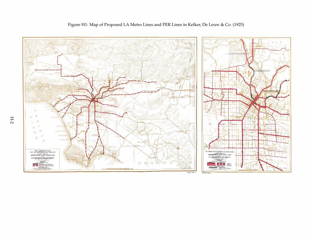
Figure H1: Map of Proposed LA Metro Lines and PER Lines in Kelker, De Leuw & Co. (1925)

H-2

Figure H2: LA Metro Rail Ridership, 1990-2000

H-3

Figure H3: LA Metro Rail Ridership, 1990-2014

H-4

Figure H4: Glossary of variables and parameters

Parameters Interpretation

ε Homogeneity of location preferences (and wage elasticity of labor supply)ζ Household expenditure share on non-housing goods

ζ = −ε(1− ζ) Price elasticity of housing demandα Share of (production) income spent on labor

α = α− 1 Inverse wage elasticity of labor demandφ Share of housing income spent on landψ Congestive cost of housing

ψ = ψφ Inverse price elasticity of housing supplyκ Semi-elasticity of commuting with respect to travel timeρ Spatial decay for instrumental variable constructionλx Treatment effect for outcome x

Variables Interpretation

A Workplace productivityB = TBε Gross residential amenity

B Simple residential amenityT Mean residential utilityC Inverse housing efficiencyC Housing productivityD Mean utility commute (net of time)E Workplace amenity (net of wage)C ConsumptionH Housing quantityW WageQ Housing price

δ = eκτ Commuting frictionτ Travel timeπ Commuting shareN Aggregate populationNY Employment at place of workLY Land used for productionM Housing materialsLH Land used for housingPM Price of housing materials

PL = (H/LH)ψ Price of land

H-5

Figure H5: Timeline of transportation in Los Angeles

1925 Comprehensive Rapid Transit Plan for the County of Los Angeles, Kelker, De Leuw & Co.developed at the request of local governments

1951 Los Angeles Metropolitan Transit Authority (LAMTA) formed1961 Pacific Electric (Red Cars) end of service1963 Los Angeles Railway (Yellow Cars) end of service1964 Southern California Rapid Transit District (SCRTD) formed from LAMTA

3/24/1985 Ross Dress for Less methane explosion in Wilshire-Fairfax1985 Construction begins on LA Metro Rail

11/20/1985 Department of Transportation and Related Agencies Appropriation Act (1986) includes lan-guage prohibiting funding of tunnels for transit along Wilshire corridor due to concernsabout methane (HR 3244)

7/14/1990 Blue Line opens2/15/1991 Metro Center station opens

1993 Los Angeles County Metropolitan Transportation Authority forms from SCRTD1/30/1993 Red Line opens, connects system to Union Station10/14/1993 Century Freeway (I-105) opens8/12/1995 Green Line opens in median of Century Freeway7/13/1996 Red Line expands to Wilshire/Vermont6/12/1999 Red Line expands to Hollywood/Vine6/24/2000 Red Line expands to North Hollywood7/26/2003 Gold Line opens

2006 Purple Line renamed from Red Line branch9/20/2006 HR 3244 amended to remove prohibitions on funding of tunnels for transit along Wilshire

corridor11/15/2009 Gold Line expands in East LA

4–6/2012 Expo Line opens3/5/2016 Gold Line expands to Azusa

5/20/2016 Expo Line expands to Santa Monica

H-6

Figure H6: Robustness to different distance bin assumptions

Effect of a single treatment under various definitions of i) as estimated by Equation (2). P represents thedistance from a station to the exterior perimeter of the tract if the tract does not contain a station and is zeroif the tract contains a station; in the main text it is zero. C represents the second criterion of i) in the maintext, the limiting centroid distance; it is 500m in the main text.

H-7

Table H1: Descriptive statistics on transportation in Los Angeles and station placement

LA County Full Sample

(1) (2) (3) (4)

A. Pre-treatment mode choice characteristics (1990)% workers commuting via: Drive alone 71.8% 74.5%% workers commuting via: Carpool 15.8% 15.8%% workers commuting via: Bus 6.9% 4.6%

B. Commuting characteristicsCommute time (minutes, 1990) 26.3 [16.8]Commute time (minutes, 2000) 28.0 [18.3]

Centroid Any Centroid AnyC. % of pre-treatment population that becomes treated < 500m < 500m < 500m < 500m

% workers at POW tract that receive treatment 11.3% 19.4% 7.2% 12.3%% workers at RES tract that receive treatment 2.6% 8.1% 1.6% 4.8%% workers that receive transit connection RES-POW 0.6% 2.9% 0.4% 1.7%

Data from Census micro records (from IPUMS) and 1990 CTPP. LA County restricts analysis to workers both living andresiding in Los Angeles county, while the full sample includes all five counties in the main sample. Brackets indicate standarddeviation. Commute times are weighted by flows.

Table H2: Pre-trends in tract-level characteristics, 1970-1990

Model-relevant Other characteristics Travel characteristics

ln ln % % %HHs %Com. %Com.Res. ln ln House Coll. Pov. Moved No Use Use

Emp. #HHs HHI Value Grads Rate <5yrs Car Auto Transit(1) (2) (3) (4) (5) (6) (7) (8) (9) (10)

All TractsProximity500m

i × t 0.025 -0.032* -0.015 -0.023 -0.015*** 0.015*** -0.016*** -0.015*** 0.004 0.012***(0.020) (0.016) (0.012) (0.014) (0.003) (0.004) (0.005) (0.006) (0.005) (0.004)

N 11643 11632 11556 11383 11650 11651 11651 7774 11644 11644PER Sample

Proximity500mi × t 0.003 -0.036** -0.015 -0.042*** -0.015*** 0.012*** -0.014** -0.014** 0.004 0.012***

(0.022) (0.017) (0.014) (0.016) (0.004) (0.005) (0.006) (0.006) (0.005) (0.004)N 3696 3695 3689 3591 3696 3696 3696 2464 3696 3696

Full 1925 Plan SampleProximity500m

i × t -0.003 -0.032* -0.018 -0.023 -0.011*** 0.010** -0.012** -0.010 0.006 0.008*(0.021) (0.017) (0.013) (0.016) (0.004) (0.005) (0.006) (0.006) (0.005) (0.005)

N 2886 2886 2881 2788 2886 2886 2886 1924 2886 2886Immediate 1925 Plan Sample

Proximity500mi × t 0.023 -0.010 -0.015 -0.004 -0.007* 0.007 -0.007 -0.010 0.006 0.011**

(0.021) (0.019) (0.015) (0.019) (0.004) (0.006) (0.006) (0.007) (0.006) (0.005)N 1236 1236 1236 1158 1236 1236 1236 824 1236 1236

Subcounty-×-Year FEs Y Y Y Y Y Y Y Y Y Y

Estimates show pre-trends from 1970-1990 for tracts treated between 1990-1999, except Column (8), which covers only 1980–1990. HH is households,and HHI is household income. Data are from GeoLytics Neighborhood Change Database and reflect 2010 geographies. All regressions include tract andsubcounty-by-year fixed effects. Standard errors clustered by tract in parentheses: * p < 0.10, ** p < 0.05, *** p < 0.01

H-8

Table H3: Treatment is not related to changes in zero flows or years opened

1Nijt>0 ln(Nijt)

(1) (2) (3) (4) (5) (6) (7) (8)

O & D contain station 0.015 0.008 0.005 0.185*** 0.150** 0.098** 0.167** 0.142**(0.034) (0.031) (0.038) (0.061) (0.058) (0.040) (0.082) (0.059)

O & D <250m from station 0.005 0.000 -0.026 0.148** 0.105* 0.058 0.145* 0.128**(0.027) (0.026) (0.033) (0.061) (0.058) (0.046) (0.077) (0.065)

O & D <500m from station 0.052** 0.035 0.019 0.073 0.036 -0.009 0.030 0.013(0.024) (0.022) (0.027) (0.058) (0.053) (0.035) (0.071) (0.052)

Years Open 0.073 0.036 0.030(0.058) (0.053) (0.071)

Years Open × O & D contain station 0.004 0.027*(0.013) (0.015)

Years Open × O & D <250m from station -0.010 -0.011(0.015) (0.018)

Years Open × O & D <500m from station -0.014 -0.012(0.010) (0.013)

N 1263082 1262478 69614 291532 291110 291110 19222 19222

Control Group All AllImmed.

All All AllImmed. Immed.

‘25 Plan ‘25 Plan ‘25 PlanStandard Three-Way FEs Y Y Y Y Y Y Y YSubcounty Pair-×-Year FEs - Y Y - Y Y Y YHighway Controls - Y Y - Y Y Y Y

High-dimensional fixed effects estimates of transit on an indicator for positive flows (Columns 1-3) or log commuting flow (Columns 4-8); standardthree-way fixed effects are tract of work-by-year, tract of residence-by-year, and tract pair. Sample consists of all non-missing/singular tract pairs. Yearsopened is relative to the newest station nearest either the origin or destination, centered on 5 years (the mean value). Standard errors clustered by tractpair, tract of residence, and tract of work in parentheses: * p < 0.10, ** p < 0.05, *** p < 0.01

H-9

Table H4: Effect of transit on commuting flows by 2000 (PPML)

Full Sample History & Shocks Same Line

(1) (2) (3) (4) (5) (6) (7) (8)

O & D contain station 0.135** 0.164** 0.125* 0.107 0.131* 0.163** 0.207* 0.152(0.069) (0.074) (0.065) (0.068) (0.068) (0.081) (0.123) (0.125)

O & D <250m from station 0.135** 0.101 0.129* 0.122* 0.120 0.210** 0.158(0.067) (0.062) (0.067) (0.068) (0.079) (0.093) (0.103)

O & D <500m from station 0.129** 0.077 0.084* 0.071 0.063 0.096 0.101(0.058) (0.049) (0.050) (0.051) (0.057) (0.070) (0.077)

N 1261978 1261978 1259440 407832 310924 69596 26270 12172

Control Group All All All PERFull Immed. Ever Treated

‘25 Plan ‘25 Plan Treated by 2000Standard Three-Way FEs Y Y Y Y Y Y Y YSubcounty Pair-×-Year FEs - - Y Y Y Y Y YHighway Controls - - Y Y Y Y Y Y

High-dimensional fixed effects estimates of λD with PPML estimator; standard three-way fixed effects are tract of work-by-year, tractof residence-by-year, and tract pair. Outcome is commuting flow. Treatment variables are mutually exclusive. Column titles definetreatment: tracts pairs on any lines are treated in Columns (1)-(6), while only tract pairs on the same line are treated in Columns (7) and(8). Standard errors clustered by tract pair, tract of residence, and tract of work in parentheses: * p < 0.10, ** p < 0.05, *** p < 0.01

H-10

Table H5: Effects are larger for tract pairs on same line

(1) (2) (3) (4) (5) (6)

O & D contain stationSame line 0.151*** 0.163*** 0.144*** 0.153*** 0.192*** 0.205***

(0.053) (0.053) (0.051) (0.055) (0.058) (0.071)

Not same line 0.026 0.035 0.040 0.056 0.087 0.075(0.076) (0.077) (0.076) (0.084) (0.082) (0.088)

O & D <250m from stationSame line 0.094 0.064 0.096 0.115* 0.145**

(0.058) (0.060) (0.062) (0.062) (0.071)

Not same line 0.046 0.049 0.087 0.095 0.105(0.059) (0.059) (0.062) (0.064) (0.079)

O & D <500m from stationSame line 0.032 0.015 0.048 0.046 0.041

(0.044) (0.042) (0.046) (0.048) (0.060)

Not same line -0.069 -0.072 -0.037 -0.051 -0.048(0.046) (0.044) (0.046) (0.046) (0.056)

N 291532 291532 291110 99480 74408 19222

Control Group All All All PER Full Immed.‘25 Plan ‘25 Plan

Standard Three-Way FEs Y Y Y Y Y YSubcounty Pair-×-Year FEs - - Y Y Y YHighway Controls - - Y Y Y Y

High-dimensional fixed effects estimates of λD with log-linear estimator; standard three-wayfixed effects are tract of work-by-year, tract of residence-by-year, and tract pair. Outcome is logcommuting flow. Treatment variables are mutually exclusive. Standard errors clustered by tractpair, tract of residence, and tract of work in parentheses: * p < 0.10, ** p < 0.05, *** p < 0.01

H-11

Table H6: Interactions of residential and workplace station proximity

(1) (2)

D contains D<250m from D<500m from D contains D<250m from D<500m fromstation station station station station station

O contains station 0.094** 0.146* -0.144* 0.108* 0.171* -0.197**(0.038) (0.077) (0.076) (0.063) (0.100) (0.094)

O<250m from station 0.021 0.017 0.043 0.096 0.118 0.051(0.059) (0.074) (0.103) (0.075) (0.110) (0.111)

O<500m from station 0.009 -0.012 0.034 0.087 0.083 0.056(0.049) (0.060) (0.047) (0.063) (0.084) (0.069)

N 291110 19222

Control Group All Immediate ‘25 PlanStandard Three-Way FEs Y YSubcounty Pair-×-Year FEs Y YHighway Control Y Y

High-dimensional fixed effects estimates of λD with log-linear estimator; standard three-way fixed effects are tract of work-by-year, tract of residence-by-year, and tract pair. Outcome is log commuting flow. Treatment variables. Standard errors clustered by tract pair, tract of residence, and tract ofwork in parentheses: * p < 0.10, ** p < 0.05, *** p < 0.01

H-12

Table H7: Bartik tests from Goldsmith-Pinkham, Sorkin, and Swift (2020), no subcounty fixedeffects

Panel A: Negative and positive weights

Sum Mean Share

Negative -0.245 -0.035 0.164Positive 1.245 0.113 0.836

Panel B: Correlations of Industry Aggregates

αk gk βk Fk Var(zk)

αk 1gk 0.043 1βk 0.132 0.463 1Fk 0.148 -0.178 -0.477 1Var(zk) 0.490 -0.112 -0.047 -0.025 1

Panel C: Top 5 Rotemberg weight industries

αk gk βk 95 % CI Ind Share

Manufacturing (durable) 0.395 -0.058 3.526 N/A 13.135Transportation 0.226 -0.110 0.558 (-1.6,2.0) 4.141FIRE 0.193 0.106 2.248 (-0.4,12.4) 7.805Personal Services 0.124 0.178 5.181 (2.4,22.6) 3.565Wholesale Trade 0.112 -0.058 -0.897 (-2.5,0.2) 4.919

Panel D: Estimates of βk for positive and negative weights

α-weighted Share ofsum overall β Mean

Negative -0.315 -0.126 1.730Positive 2.827 1.126 1.985

Panel E: Alternative estimates and overidentification

Bartik TSLS LIML MBTSLS HFUL

∆ ln(Wjt) 2.512 1.457 2.911 1.571 2.470(1.094) (0.662) (1.835) (0.705) (5.065)

Over ID Test Stat. 34.2 22.2 23.9p-value [0.01] [0.14] [0.09]

This table reports statistics about Rotemberg weights and alternate IV estimators as suggested inGoldsmith-Pinkham, Sorkin, and Swift (2020). The results correspond to Table 3 column 5. In allcases, statistics reflect normalized growth rates. Panel A reports the share and sum of negativeRotemberg weights. Panel B reports correlations between the weights (αk), the national compo-nent of growth (gk), the just-identified coefficient estimates (βk), the first-stage F-statistic of theindustry share (Fk), and the variation in the industry shares across locations (VAR(zk)). Panel Creports variation in the weights across years. Panel D reports the top five industries according tothe Rotemberg weights. The 95% CI uses the weak-instrument robust CI from Chernozhukov andHansen (2008) over a range from -25 to 25 and is N/A if it exceeds that range, and Ind Share is theindustry share (multiplied by 100). Panel E reports a variety of alternative estimates. TSLS useseach industry share separately as instruments. LIML reports estimates using the limited informa-tion maximum likelihood estimator with the same set of instruments. MBTSLS uses Anatolyev(2013) and Kolesár et al. (2015) with the same set of instruments. HFUL uses the HFUL estimator(Hausman et al. 2012) with the same set of instruments, and the J-statistic from Chao et al. (2014).p-values are in brackets.

H-13

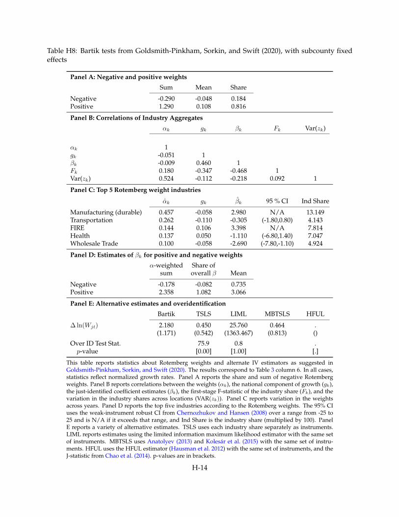
Table H8: Bartik tests from Goldsmith-Pinkham, Sorkin, and Swift (2020), with subcounty fixedeffects

Panel A: Negative and positive weights

Sum Mean Share

Negative -0.290 -0.048 0.184Positive 1.290 0.108 0.816

Panel B: Correlations of Industry Aggregates

αk gk βk Fk Var(zk)

αk 1gk -0.051 1βk -0.009 0.460 1Fk 0.180 -0.347 -0.468 1Var(zk) 0.524 -0.112 -0.218 0.092 1

Panel C: Top 5 Rotemberg weight industries

αk gk βk 95 % CI Ind Share

Manufacturing (durable) 0.457 -0.058 2.980 N/A 13.149Transportation 0.262 -0.110 -0.305 (-1.80,0.80) 4.143FIRE 0.144 0.106 3.398 N/A 7.814Health 0.137 0.050 -1.110 (-6.80,1.40) 7.047Wholesale Trade 0.100 -0.058 -2.690 (-7.80,-1.10) 4.924

Panel D: Estimates of βk for positive and negative weights

α-weighted Share ofsum overall β Mean

Negative -0.178 -0.082 0.735Positive 2.358 1.082 3.066

Panel E: Alternative estimates and overidentification

Bartik TSLS LIML MBTSLS HFUL

∆ ln(Wjt) 2.180 0.450 25.760 0.464 .(1.171) (0.542) (1363.467) (0.813) ()

Over ID Test Stat. 75.9 0.8 .p-value [0.00] [1.00] [.]

This table reports statistics about Rotemberg weights and alternate IV estimators as suggested inGoldsmith-Pinkham, Sorkin, and Swift (2020). The results correspond to Table 3 column 6. In all cases,statistics reflect normalized growth rates. Panel A reports the share and sum of negative Rotembergweights. Panel B reports correlations between the weights (αk), the national component of growth (gk),the just-identified coefficient estimates (βk), the first-stage F-statistic of the industry share (Fk), and thevariation in the industry shares across locations (VAR(zk)). Panel C reports variation in the weightsacross years. Panel D reports the top five industries according to the Rotemberg weights. The 95% CIuses the weak-instrument robust CI from Chernozhukov and Hansen (2008) over a range from -25 to25 and is N/A if it exceeds that range, and Ind Share is the industry share (multiplied by 100). PanelE reports a variety of alternative estimates. TSLS uses each industry share separately as instruments.LIML reports estimates using the limited information maximum likelihood estimator with the same setof instruments. MBTSLS uses Anatolyev (2013) and Kolesár et al. (2015) with the same set of instru-ments. HFUL uses the HFUL estimator (Hausman et al. 2012) with the same set of instruments, and theJ-statistic from Chao et al. (2014). p-values are in brackets.

H-14

Table H9: Transit and non-commuting fundamentals with half spatial decay

d = 500m d = 1km

(1) (2) (3) (4) (5) (6) (7) (8)

Effect on productivityI.) λA estimated using ∆A = ∆A− µ∆ ln(ΥFar)

Proximityi × t 0.031 0.030 0.017 0.021 0.040 0.041 0.027 0.035(0.039) (0.039) (0.038) (0.043) (0.037) (0.038) (0.037) (0.043)

N 2469 1167 934 394 2469 1167 934 394

Effect on residential amenity levelIV.) λB estimated using ∆B = ∆B − η∆ ln(ΩFar)

Proximityi × t 0.050 0.068** 0.045 0.007 0.035 0.056* 0.025 -0.028(0.032) (0.033) (0.033) (0.035) (0.029) (0.031) (0.030) (0.034)

N 2149 994 815 343 2149 994 815 343

Control Group All PERFull Immed.

All PERFull Immed.

‘25 Plan ‘25 Plan ‘25 Plan ‘25 Plan

Results from sixteen regressions of transit proximity on local productivity after removing agglomeration. Here, thedistance effect of agglomeration decays at half the values in Ahlfeldt et al. (2015). All regressions include tract fixedeffects, subcounty-by-year fixed effects, and controls. Controls include changes in highway proximity and 1990 levelsof log household income, share of residents with at least a high school degree, and manufacturing employment. Samplesize reflects number of differenced tracts. Standard errors clustered by tract in parentheses: * p < 0.10, ** p < 0.05, ***p < 0.01

H-15

Table H10: Transit and non-mutable fundamentals

∆Yit

d = 500m d = 1km

(1) (2) (3) (4) (5) (6) (7) (8)

A. Effect on inverse housing supply efficiency ∆C, λC

Proximityi × t 0.006 0.007 -0.024 -0.041 0.007 0.012 -0.031 -0.053(0.049) (0.051) (0.051) (0.058) (0.044) (0.047) (0.048) (0.057)

N 2172 996 818 348 2172 996 818 348

B. Effect on workplace amenity ∆E, λE

Proximityi × t -0.016 -0.083 -0.064 -0.115 -0.004 -0.087 -0.062 -0.138*(0.070) (0.072) (0.075) (0.084) (0.066) (0.069) (0.072) (0.084)

N 2516 1168 935 395 2516 1168 935 395

Control Group All PERFull Immed.

All PERFull Immed.

‘25 Plan ‘25 Plan ‘25 Plan ‘25 Plan

Results from sixteen regressions of transit proximity on local fundamentals. All regressions include tract fixed effects,subcounty-by-year fixed effects, and controls. Controls include changes in highway proximity and 1990 levels of loghousehold income, share of residents with at least a high school degree, and manufacturing employment. Sample sizereflects number of differenced tracts. Standard errors clustered by tract in parentheses: * p < 0.10, ** p < 0.05, ***p < 0.01

H-16

Table H11: Transit, income change, and land use change (robustness)

∆Yit

d = 500m d = 1km

(1) (2) (3) (4) (5) (6) (7) (8)

A. Change in residential land

Proximityi × t 0.006*** 0.002 0.001 0.001 0.007*** 0.003 0.002 0.001(0.002) (0.001) (0.001) (0.001) (0.002) (0.002) (0.002) (0.002)

N 2468 1152 920 385 2468 1152 920 385

B. Change in household income

Proximityi × t -0.016 -0.006 -0.006 -0.019 -0.025 -0.014 -0.015 -0.034*(0.017) (0.017) (0.017) (0.018) (0.016) (0.017) (0.017) (0.019)

N 2476 1142 915 380 2476 1142 915 380

Control Group All PERFull Immed.

All PERFull Immed.

‘25 Plan ‘25 Plan ‘25 Plan ‘25 Plan

Results from sixteen regressions of transit proximity on residential land use and household income. All regressions in-clude tract fixed effects, subcounty-by-year fixed effects, and controls. Controls include changes in highway proximityand 1990 levels of log household income, share of residents with at least a high school degree, and manufacturing em-ployment. Sample size reflects number of differenced tracts. Standard errors clustered by tract in parentheses: * p < 0.10,** p < 0.05, *** p < 0.01

Table H12: Effect of LA Metro Rail on residential commute share using rail transit

Residential Commute Share using Rail Transit

d = 500m d = 1km

(1) (2) (3) (4) (5) (6) (7) (8)

Proximityi × t 0.0084*** 0.0081*** 0.0081*** 0.0079*** 0.0078*** 0.0077*** 0.0077*** 0.0076***(0.0015) (0.0014) (0.0014) (0.0015) (0.0012) (0.0012) (0.0013) (0.001)

N 2262 1037 848 371 2262 1037 848 371

Control Group All PERFull Immed.

All PERFull Immed.

‘25 Plan ‘25 Plan ‘25 Plan ‘25 Plan

Results from eight regressions of transit proximity on subway/light rail commute share. All regressions include tract fixed effects,subcounty-by-year fixed effects, and controls. Controls include changes in highway proximity and 1990 levels of log household income,share of residents with at least a high school degree, and manufacturing employment. Sample size reflects number of differenced tracts.Standard errors clustered by tract in parentheses: * p < 0.10, ** p < 0.05, *** p < 0.01

H-17

Table H13: Welfare effects of model extensions (% change in welfare)

GeneralPartial General Equilibrium

Equilibrium Equilibrium + Spillovers(1) (2) (3)

Baseline: Commuting Effect through 2000 0.04410 0.04404 0.04324+ Dynamic Effect (through 2015) 0.08032 0.07965 0.07838+ Congestion Effect 0.10671 0.10632 0.10431+ Dynamic & Congestion Effects 0.14295 0.14196 0.13946

Baseline & Reduced Land Use Regulation 0.12234 0.10574 0.10371+ Dynamic Effect (through 2015) 0.15859 0.14266 0.14040+ Congestion Effect 0.18500 0.16806 0.16481+ Dynamic & Congestion Effects 0.22127 0.20500 0.20153

Baseline & 5% Amenity 0.10757 0.10688 0.10478+ Dynamic Effect (through 2015) 0.14544 0.14355 0.14118+ Congestion Effect 0.17022 0.16920 0.16588+ Dynamic & Congestion Effects 0.20811 0.20589 0.20230

Baseline & 4% Productivity 0.36608 0.28847 0.28735+ Dynamic Effect (through 2015) 0.40241 0.32548 0.32400+ Congestion Effect 0.42888 0.35090 0.34857+ Dynamic & Congestion Effects 0.46524 0.38794 0.38524

This table gives the percentage change in welfare for various model scenarios (e.g., 0.04409 is a0.044% change in welfare). Columns 1–3 show partial equilibrium results, general equilibrium re-sults that ignore endogenous agglomeration, and general equilibrium results that account for en-dogenous agglomeration. Partial equilibrium reflects only changes in items that feed into the utilityfunction, but no feedbacks (but effects to A and C do have price effects). The first panel includesthe results in the main paper, whereas the other panels present experiments presuming other effectsbecome present: Reduced Land Use Regulation assumes λC = −0.3297 just in tracts containingtransit stations, such that residential density increases in those locations by 10%; 5% Amenity as-sumes λB = 0.05 with the 500m proximity measure of treatment; and 4% Productivity assumesλA = 0.04 with the 500m proximity measure of treatment.

H-18